Asymptotic Distribution-free Change-point Detection for Modern Data Based on a New Ranking Scheme

Abstract

Change-point detection (CPD) involves identifying distributional changes in a sequence of independent observations. Among nonparametric methods, rank-based methods are attractive due to their robustness and effectiveness and have been extensively studied for univariate data. However, they are not well explored for high-dimensional or non-Euclidean data. This paper proposes a new method, Rank INduced by Graph Change-Point Detection (RING-CPD), which utilizes graph-induced ranks to handle high-dimensional and non-Euclidean data. The new method is asymptotically distribution-free under the null hypothesis, and an analytic $p$-value approximation is provided for easy type-I error control. Simulation studies show that RING-CPD effectively detects change-points across a wide range of alternatives and is also robust to heavy-tailed distribution and outliers. The new method is illustrated by the detection of seizures in a functional connectivity network dataset and travel pattern changes in the New York City Taxi dataset.

I Introduction

Given a sequence of independent observations, an important problem is to decide whether the observations are from the same distribution or there is a change of distribution at a certain time point. Change-point detection (CPD) has attracted a lot of interest since the seminal work of [1]. In this big data era, it has diverse applications in many fields, including functional magnetic resonance recordings [2, 3], healthcare [4, 5], communication network evolution [6, 7, 8], and financial modeling [9, 10]. Parametric approaches (see for example, [11, 12, 13, 14, 15]) are useful to address the problem for univariate and low-dimensional data, however, they are limited for high-dimensional or non-Euclidean data due to a large number of parameters to be estimated unless strong assumptions are imposed.

A few nonparametric methods have been proposed, including kernel-based methods [16, 17, 18, 19, 20], interpoint distance-based methods [21, 22] and graph-based methods [23, 24, 25, 26, 27, 28, 29]. Note that the graph-based methods proposed in [25] take into account the curse of dimensionality [30] and can detect a wide range of changes. These graph-based CPD methods are promising approaches due to their flexibility and efficiency in analyzing high-dimensional and non-Euclidean data. However, the graph-based methods focused on unweighted graphs, which may cause information loss. Later, [22] adopted a similar idea and proposed an asymptotic distribution-free approach utilizing all interpoint distances that worked well for detecting both location and scale changes. However, their test statistics are time and memory-consuming, and implicitly require the existence of the second moment of the underlying distribution, which can be violated by heavy-tailed data or outliers that are common in many applications.

Among the nonparametric methods, rank-based methods are attractive for univariate data due to their robustness and effectiveness [31, 32, 33, 34, 35, 36, 37, 38]. However, they are less explored for high-dimensional or non-Euclidean data. Specifically, existing multivariate rank-based methods are limited in many ways. For instance, [39] proposed to use the component-wise rank, which requires the dimension of the data to be smaller than the number of observations and suffers from dependent covariates. [40] and [41] proposed the spatial rank-based methods, which were designed mainly for detecting mean shifts. [42] proposed to use the ranks obtained from data depths, which is often used for low-dimensional data and is computation-extensive when the dimension is high.

Noticing the gap between the potential benefit of the rank-based method and the scarce exploration for multivariate/high-dimensional data, we propose a new rank-based method called Rank INduced by Graph Change-Point Detection (RING-CPD), which can be applied to high-dimensional and non-Euclidean data. Unlike previous works dealing with the ranks of observations that are often limited to low-dimensional distributions, we propose to use the rank induced by similarity graphs that can be applied to data with dimension much larger than the sample size. The graph-induced rank [43] is the rank defined in the similarity graphs. Instead of treating all edges in the graph equally, we assign the rank as weights to each edge and construct the scan statistic based on the ranks. Discussions on this rank and the new test are presented in Section II. We prove that the proposed scan statistic is asymptotic distribution-free, facilitating its usage to a broader community of researchers and analysts. The proposed statistic can work for a wide range of alternatives and are robust to heavy-tailed distribution and outliers, as illustrated by extensive simulation studies in Section IV and two real data examples in Section V. The details of proofs of the theorems are deferred to the Supplementary Material.

II Method

For a sequence of independent observations $\big{\{}y_{i}\big{\}}_{i=1}^{n}$, we consider testing

$$H_{0}:y_{i}\sim F_{0},\quad i=1,\ldots,n$$

against the single change-point alternative

$$H_{1}:\exists 1\leq\tau<n,y_{i}\sim\begin{cases}F_{0},&i\leq\tau,\\ F_{1},&\text{ otherwise }\end{cases}$$

or the changed interval alternative

$$H_{2}:\exists 1\leq\tau_{1}<\tau_{2}\leq n,\quad y_{i}\sim\begin{cases}F_{0},&i=\tau_{1}+1,\ldots,\tau_{2},\\ F_{1},&\text{ otherwise,}\end{cases}$$

where $F_{0}$ and $F_{1}$ are two different distribution. When there are multiple change-points, the two alternatives can be applied recursively. Alternatively, our method in the following can be extended similarly to [44] to accommodate multiple change-points, using the idea of wild binary segmentation [45] or seeded binary segmentation [46]. We utilize the graph-induced rank proposed by [43]:

$$R_{ij}=\sum_{l=1}^{k}\mathbbm{1}\big{(}(i,j)\in G_{l}\big{)}\,,$$

where $\mathbbm{1}(\cdot)$ is the indicator function, $\{G_{l}\}_{l=1}^{k}$ is a sequence of similarity graphs with nodes $\{y_{i}\}_{i=1}^{n}$ and edges constructed inductively:

$$G_{l+1}=G_{l}\cup G_{l+1}^{*}\,\text{ with }G_{l+1}^{*}=\arg\max_{G^{\prime}\in\mathcal{G}_{l+1}}\sum_{(i,j)\in G^{\prime}}S_{ij},$$

where $\mathcal{G}_{l+1}=\{G^{\prime}\in\mathcal{G}:G^{\prime}\cap G_{l}=\emptyset\}$ and $\mathcal{G}$ is a graph set with elements satisfying specific user-defined constraints, $S_{ij}=S(Z_{i},Z_{j})$ measures the similarity between $Z_{i}$ and $Z_{j}$. For example, $S(Z_{i},Z_{j})$ could be the negative Euclidean distance between $Z_{i}$ and $Z_{j}$ if the data lies in the Euclidean space. It could also be some other user-defined quantities where more similar observations tend to have larger values. Many graphs such as the $k$-nearest neighbor graph ($k$-NNG) and the $k$-minimum spanning tree ($k$-MST) [47] satisfy the above definition of the sequence of graphs. For example, for NNG, the structure constraint on $G^{\prime}$ is that each node $i$ only points out to one of the other nodes. As a result, $G_{l}$ is the $l$-NNG, $G_{l+1}^{*}$ is the $(l+1)$th NNG and $G_{l+1}$ is the $(l+1)$-NNG. For $k$-MST, the constraint is that $G^{\prime}$ should be a tree connecting all observations, making $G_{l}$ the $l$-MST, $G_{l+1}^{*}$ the $(l+1)$th MST and $G_{l+1}$ the $(l+1)$-MST. For more choices of graphs, see [43]. The graph-induced ranks impose more weights on the edges with higher similarity, thus incorporating more similarity information than the unweighted graph. In the meantime, the robustness property of the ranks makes the weights less sensitive to outliers compared to direct using distance. The behavior of the graph-induced rank matrix in the $10$-NNG is illustrated in Figure 1 by simulated data. Based on the ranks, we define two basic quantities

$$U_{1}(t_{1},t_{2})=\sum_{i=1}^{n}\sum_{j=1}^{n}R_{ij}\mathbbm{1}(t_{1}<i,j\leq t_{2})\text{ and }U_{2}(t_{1},t_{2})=\sum_{i=1}^{n}\sum_{j=1}^{n}R_{ij}\mathbbm{1}(i,j\leq t_{1}\text{ or }i,j>t_{2})\,.$$ (1)

For derivation simplicity, we symmetrize $\mathbf{R}=(R_{ij})_{i,j=1}^{n}$ by $0.5(\mathbf{R}+\mathbf{R}^{\scriptscriptstyle\sf T})$. Note that this symmetrization does not change the value of $U_{1}$ and $U_{2}$. Without further specialization, we use $\mathbf{R}$ to denote its symmetrized version in the following. We use ${\mathbbm{E}}$, ${\rm Var}$, and ${\rm Cov}$ to respectively denote the expectation, variance, and covariance under the permutation null distribution, which places $1/n!$ probability on each of the $n!$ permutations of the order of the observations. We propose to use the following max-type statistic

$$M_{R}(t_{1},t_{2})=\max\big{(}Z_{w}(t_{1},t_{2}),|Z_{\mathrm{diff}}(t_{1},t_{2})|\big{)}\,,$$ (2)

where

$$Z_{w}(t_{1},t_{2})=\frac{U_{w}(t_{1},t_{2})-{\mathbbm{E}}\big{(}U_{w}(t_{1},t_{2})\big{)}}{\sqrt{{\rm Var}\big{(}U_{w}(t_{1},t_{2})\big{)}}}\text{ and }Z_{\mathrm{diff}}(t_{1},t_{2})=\frac{U_{\mathrm{diff}}(t_{1},t_{2})-{\mathbbm{E}}\big{(}U_{\mathrm{diff}}(t_{1},t_{2})\big{)}}{\sqrt{{\rm Var}\big{(}U_{\mathrm{diff}}(t_{1},t_{2})\big{)}}}\,,$$

with $U_{\mathrm{diff}}(t_{1},t_{2})=U_{1}(t_{1},t_{2})-U_{2}(t_{1},t_{2})$ and

$$U_{w}(t_{1},t_{2})=\frac{n-t_{2}+t_{1}-1}{n-2}U_{1}(t_{1},t_{2})+\frac{t_{2}-t_{1}-1}{n-2}U_{2}(t_{1},t_{2})\,.$$

The explicit expressions of ${\mathbbm{E}}\big{(}U_{1}(t_{1},t_{2})\big{)}$, ${\mathbbm{E}}\big{(}U_{2}(t_{1},t_{2})\big{)}$ and $\bm{\Sigma}(t_{1},t_{2})$ are presented in Lemma 1. Let

$$\bar{R}_{i\cdot}=\frac{\sum_{j=1}^{n}R_{ij}}{n-1}\,,r_{0}=\frac{\sum_{i=1}^{n}\bar{R}_{i\cdot}}{n}\,,r_{1}^{2}=\frac{\sum_{i=1}^{n}\bar{R}_{i\cdot}^{2}}{n}\,,r_{d}^{2}=\frac{\sum_{i=1}^{n}\sum_{j=1}^{n}R_{ij}^{2}}{n(n-1)}\,,V_{d}=r_{d}^{2}-r_{0}^{2}\,,V_{r}=r_{1}^{2}-r_{0}^{2}\,.$$

Lemma 1

Under the permutation null distribution, we have

$${\mathbbm{E}}\big{(}U_{1}(t_{1},t_{2})\big{)} =(t_{2}-t_{1})(t_{2}-t_{1}-1)r_{0}\,,$$

$${\mathbbm{E}}\big{(}U_{2}(t_{1},t_{2})\big{)} =(n-t_{2}+t_{1})(n-t_{2}+t_{1}-1)r_{0}$$

$${\rm Var}\big{(}U_{1}(t_{1},t_{2})\big{)} =f_{1}(t_{2}-t_{1})V_{d}+f_{2}(t_{2}-t_{1})V_{r}\,,$$

$${\rm Var}\big{(}U_{2}(t_{1},t_{2})\big{)} =f_{1}(n-t_{2}+t_{1})V_{d}+f_{2}(n-t_{2}+t_{1})V_{r}\,,$$

$${\rm Cov}\big{(}U_{1}(t_{1},t_{2}),U_{2}(t_{1},t_{2})\big{)} =f_{1}(t_{2}-t_{1})\big{(}V_{d}-2(n-1)V_{r}\big{)}\,,$$

where

$$f_{1}(t)=\frac{2t(t-1)(n-t)(n-t-1)}{(n-2)(n-3)}\text{ and }f_{2}(t)=\frac{4t(n-t)(t-1)(t-2)(n-1)}{(n-2)(n-3)}\,.$$

The proof of Lemma 1 is through combinatorial analysis. It can be done similarly to the proof of Theorem $2.1$ in [43] and thus omitted here.

Let $M_{R}(t)=M_{R}(0,t)$. We reject $H_{0}$ against $H_{1}$, if the scan statistic

$$\max_{n_{0}\leq t\leq n_{1}}M_{R}(t)$$ (3)

exceeds the critical value for a given nominal level. We reject $H_{0}$ against $H_{2}$, if the scan statistic

$$\max_{1\leq t_{1}<t_{2}\leq n\atop n_{0}\leq t_{2}-t_{1}\leq n_{1}}M_{R}(t_{1},t_{2})$$ (4)

is large enough. Here $n_{0}$ and $n_{1}$ are pre-specified integers. A common choice of $n_{0}$ and $n_{1}$ is $n_{0}=[0.05n]$ and $n_{1}=n-n_{0}$, where $[x]$ denotes the integer closest to $x$. Under the alternative hypothesis, it is possible that (i) both $U_{1}(t_{1},t_{2})$ and $U_{2}(t_{1},t_{2})$ are larger than their null expectations (a typical scenario under location alternatives) and (ii) one of them is larger than while the other one is smaller than its corresponding null expectation (a typical scenario under scale alternatives). See [30] for more discussions on these scenarios. For (i), $Z_{w}(t_{1},t_{2})$ will be large and for (ii), $|Z_{\mathrm{diff}}(t_{1},t_{2})|$ will be large. Thus, $M_{R}$ is powerful for different types of alternatives. To illustrate the behaviors of $Z_{w}$, $Z_{\mathrm{diff}}$ and $M_{R}$ under different scenarios, we generate $n=200$ independent multivariate observations with dimension $d=500$ from

• (Null) $y_{i}\sim N(\mathbf{0}_{d},\mathbf{1}_{d}),i=1,\ldots,n$;

• (Location shift) $y_{i}\sim N(\mathbf{0}_{d},\mathbf{I}_{d}),i=1,\ldots,3n/4$, $y_{i}\sim N(0.21\mathbf{1}_{d},\mathbf{I}_{d}),i=3n/4+1,\ldots,n$;

• (Scale shift) $y_{i}\sim N(\mathbf{0}_{d},\mathbf{I}_{d}),i=1,\ldots,n/4$, $y_{i}\sim N(\mathbf{0}_{d},1.2\mathbf{I}_{d}),i=n/4+1,\ldots,n$;

• (Location and scale mixed shift) $y_{i}\sim N(\mathbf{0}_{d},\mathbf{I}_{d}),i=1,\ldots,n/2$, $y_{i}\sim N(0.1\mathbf{1}_{d},1.2\mathbf{I}_{d}),i=n/2+1,\ldots,n$.

For all numeric experiments in the paper, we use the negative Euclidean norm as the similarity measure unless specifically noted. The values of $Z_{w}(t)=Z_{w}(0,t)$, $|Z_{\mathrm{diff}}(t)|=|Z_{\mathrm{diff}}(0,t)|$ and $M_{R}(t)$ against $t$ are presented in Figure 1.

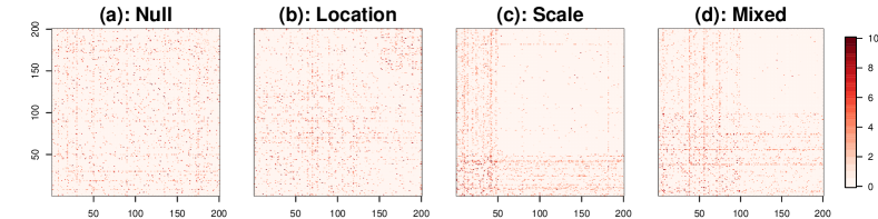
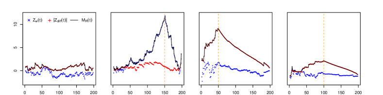
Figure 1: Top panel: heatmap of the graph-induced rank matrix $\mathbf{R}$ in $10$-NNG. Bottom panel: the values of $Z_{w}(t)=Z_{w}(0,t)$ (blue), $|Z_{\mathrm{diff}}(t)|=|Z_{\mathrm{diff}}(0,t)|$ (red) and $M_{R}(t)$ (black) against $t$ under different scenarios. The true change points are denoted by the vertical dashed lines (orange).

III Asymptotic distribution of the scan statistics

For decision-making, the critical values should be determined. Alternatively, we consider the tail probabilities

$${\mathbbm{P}}\big{(}\max_{n_{0}\leq t\leq n_{1}}M_{R}(t)>b\big{)}$$ (5)

for the single change-point alternative and

$${\mathbbm{P}}\big{(}\max_{1\leq t_{1}<t_{2}\leq n\atop l_{0}\leq t_{2}-t_{1}\leq l_{1}}M_{R}(t_{1},t_{2})>b\big{)}$$ (6)

for the changed interval alternative, respectively, where ${\mathbbm{P}}$ denotes the probability under the permutation null distribution. When $n$ is small, we can apply the permutation procedure. However, it is time-consuming when $n$ is large. Hence, we derive the asymptotic distribution of the scan statistics for analytic approximations of the tail probabilities.

III-A Asymptotic null distributions of the basic processes

By the definition of $M_{R}(t)$ and $M_{R}(t_{1},t_{2})$, it is sufficient to derive the limiting distributions of

$$\big{\{}Z_{\mathrm{diff}}(\lfloor nu\rfloor):0<u<1\big{\}}\text{ and }\big{\{}Z_{w}(\lfloor nu\rfloor):0<u<1\big{\}}$$ (7)

for the single change-point alternative and

$$\big{\{}Z_{\mathrm{diff}}(\lfloor nu\rfloor,\lfloor nv\rfloor):0<u<v<1\big{\}}\text{ and }\big{\{}Z_{w}(\lfloor nu\rfloor,\lfloor nv\rfloor):0<u<v<1\big{\}}$$ (8)

for the changed-interval alternative, where $\lfloor x\rfloor$ denotes the largest integer less than or equal to $x$. We use the notations $a_{n}=o(b_{n})$ and $a_{n}\prec b_{n}$ when $\lim_{n\rightarrow\infty}a_{n}/b_{n}=0$, and $a_{n}\precsim b_{n}$ when $\lim_{n\rightarrow\infty}a_{n}/b_{n}$ is bounded. The proof of Theorem 1 is provided in Supplement S1.

Theorem 1

Under Conditions (1) $r_{1}\prec r_{d}$; (2) $\sum_{i=1}^{n}\big{(}\sum_{j=1}^{n}R_{ij}^{2}\big{)}^{2}\precsim n^{3}r_{d}^{4}$; (3) $\sum_{i=1}^{n}\big{|}\widetilde{R}_{i\cdot}\big{|}^{3}\prec(nV_{r})^{1.5}$; (4) $\sum_{i=1}^{n}\widetilde{R}_{i\cdot}^{3}\prec nr_{d}V_{r}$; (5) $\big{|}\sum_{i=1}^{n}\sum_{j\neq s}^{n}R_{ij}R_{is}\widetilde{R}_{j\cdot}\widetilde{R}_{s\cdot}\big{|}\prec n^{3}r_{d}^{2}V_{r}$; (6) $\sum_{i=1}^{n}\sum_{j=1}^{n}\sum_{s,l\neq i,j}^{n}R_{ij}R_{js}R_{sl}R_{li}\prec n^{4}r_{d}^{4}$, we have

1. $\big{\{}Z_{\mathrm{diff}}(\lfloor nu\rfloor):0<u<1\big{\}}$ and $\big{\{}Z_{w}(\lfloor nu\rfloor):0<u<1\big{\}}$ converge to independent Gaussian processes in finite dimensional distributions, which we denote as $\big{\{}Z_{\mathrm{diff}}^{*}(u):0<u<1\big{\}}$ and $\big{\{}Z_{w}^{*}(u):0<u<1\big{\}}$, respectively.

2. $\big{\{}Z_{\mathrm{diff}}(\lfloor nu\rfloor,\lfloor nv\rfloor):0<u<v<1\big{\}}$ and $\big{\{}Z_{w}(\lfloor nu\rfloor,\lfloor nv\rfloor):0<u<v<1\big{\}}$ converge to independent two-dimension Gaussian random fields in finite dimensional distributions, which we denote as $\big{\{}Z_{\mathrm{diff}}^{*}(u,v):0<u<v<1\big{\}}$ and $\big{\{}Z_{w}^{*}(u,v):0<u<v<1\big{\}}$, respectively.

Remark 1

Conditions (1)-(6) put restrictions on the similarity graph and the ranks. Importantly, they require that there should not be an excessive number of hub nodes in the graph and that the variation of the average row-wise ranks, $V_{r}$, should not be dominated by a small portion of elements. Note that these conditions are exactly the same as [43], which is exciting because we do not need extra conditions when we extend the statistics from the two-sample setting to the change-point detection setting.

Let $\rho_{w}^{*}(u,v)=\mathbf{Cov}\big{(}Z_{w}^{*}(u),Z_{w}^{*}(v)\big{)}$ and $\rho_{\mathrm{diff}}^{*}(u,v)=\mathbf{Cov}\big{(}Z_{\mathrm{diff}}^{*}(u),Z_{\mathrm{diff}}^{*}(v)\big{)}$. We present explicit formulas of $\rho_{w}^{*}(u,v)$ and $\rho_{\mathrm{diff}}^{*}(u,v)$ in Theorem 2 with the proof in Supplement S2.

Theorem 2

The exact expressions for $\rho_{\mathrm{diff}}^{*}(u,v)$ and $\rho_{w}^{*}(u,v)$ are

$$\rho_{w}^{*}(u,v) =\frac{(u\wedge v)(1-(u\vee v))}{(u\vee v)(1-(u\wedge v))}\,,$$

$$\rho_{\mathrm{diff}}^{*}(u,v) =\frac{(u\wedge v)(1-(u\vee v))}{\sqrt{(u\wedge v)(1-(u\wedge v))(u\vee v)(1-(u\vee v))}}\,,$$

where $u\wedge v=\min(u,v)$ and $u\vee v=\max(u,v)$.

Theorems 1 and 2 together show that when $\mathbf{R}$ satisfies Conditions (1)-(6), the limiting distributions of (7) and (8), and statistics based on (7) and (8), are independent from $\mathbf{R}$, thus asymptotically distribution-free.

III-B Tail probabilities

Based on Theorems 1 and 2, following the routine of [25], we can approximate the tail probabilities by

$${\mathbbm{P}}\big{(}\max_{n_{0}\leq t\leq n_{1}}M_{R}(t)>b\big{)}\approx 1-{\mathbbm{P}}\big{(}\max_{n_{0}\leq t\leq n_{1}}Z_{w}(t)<b\big{)}{\mathbbm{P}}\big{(}\max_{n_{0}\leq t\leq n_{1}}|Z_{\mathrm{diff}}(t)|<b\big{)}\,,$$ (9)

$${\mathbbm{P}}\big{(}\max_{1\leq t_{1}<t_{2}\leq n\atop l_{0}\leq t_{2}-t_{1}\leq l_{1}}M_{R}(t_{1},t_{2})>b\big{)}\approx 1-{\mathbbm{P}}\big{(}\max_{l_{0}\leq t_{2}-t_{1}\leq l_{1}}Z_{w}(t_{1},t_{2})<b\big{)}{\mathbbm{P}}\big{(}\max_{l_{0}\leq t_{2}-t_{1}\leq l_{1}}|Z_{\mathrm{diff}}(t_{1},t_{2})|<b\big{)}\,,$$ (10)

where

$${\mathbbm{P}}\big{(}\max_{n_{0}\leq t\leq n_{1}}Z_{w}(t)>b\big{)}\approx b\phi(b)\int_{\frac{n_{0}}{n}}^{\frac{n_{1}}{n}}h_{w}(n,x)\nu\big{(}b\sqrt{2h_{w}(n,x)/n}\big{)}{\rm d}x\,,$$ (11)

$${\mathbbm{P}}\big{(}\max_{l_{0}\leq t_{2}-t_{1}\leq l_{1}}Z_{w}(t_{1},t_{2})>b\big{)}\approx b^{3}\phi(b)\int_{\frac{l_{0}}{n}}^{\frac{l_{1}}{n}}\Big{(}h_{w}(n,x)\nu\big{(}b\sqrt{2h_{w}(n,x)/n}\big{)}\Big{)}^{2}(1-x){\rm d}x\,,$$ (12)

$${\mathbbm{P}}\big{(}\max_{n_{0}\leq t\leq n_{1}}Z_{\mathrm{diff}}(t)>b\big{)}\approx b\phi(b)\int_{\frac{n_{0}}{n}}^{\frac{n_{1}}{n}}h_{\mathrm{diff}}(n,x)\nu\big{(}b\sqrt{2h_{\mathrm{diff}}(n,x)/n}\big{)}{\rm d}x\,,$$ (13)

$${\mathbbm{P}}\big{(}\max_{l_{0}\leq t_{2}-t_{1}\leq l_{1}}Z_{\mathrm{diff}}(t_{1},t_{2})>b\big{)}\approx b^{3}\phi(b)\int_{\frac{l_{0}}{n}}^{\frac{l_{1}}{n}}\Big{(}h_{\mathrm{diff}}(n,x)\nu\big{(}b\sqrt{2h_{\mathrm{diff}}(n,x)/n}\big{)}\Big{)}^{2}(1-x){\rm d}x\,.$$ (14)

with

$$h_{w}(n,x)=\frac{(n-1)(2nx^{2}-2nx+1)}{2x(1-x)(nx-1)(nx-n+1)}\quad\text{ and }\quad h_{\mathrm{diff}}(n,x)=\frac{1}{2x(1-x)}\,.$$

Here $v(x)$ is approximated as $v(x)\approx(2/x)(\Phi(x/2)-0.5)/\big{(}(x/2)\Phi(x/2)+\phi(x/2)\big{)}$ [48], where $\Phi(\cdot)$ and $\phi(\cdot)$ are the standard normal cumulative density function and standard normal density function, respectively.

III-C Skewness correction

As observed by [23, 25], the analytical approximations of (9) and (10) can be improved by skewness correction when $n_{0}$ and $n-n_{1}$ decrease. It can be seen clearly in Figure 2 that $Z_{w}(t)$ and $Z_{\mathrm{diff}}(t)$ are more skewed toward the two ends. To be specific, instead of using (11)-(14) to approximate (9) and (10), we use

$${\mathbbm{P}}\big{(}\max_{n_{0}\leq t\leq n_{1}}Z_{w}(t)>b\big{)}\approx b\phi(b)\int_{\frac{n_{0}}{n}}^{\frac{n_{1}}{n}}K_{w}(nx)h_{w}(n,x)\nu\big{(}b\sqrt{2h_{w}(n,x)/n}\big{)}{\rm d}x\,,$$ (15)

$${\mathbbm{P}}\big{(}\max_{l_{0}\leq t_{2}-t_{1}\leq l_{1}}Z_{w}(t_{1},t_{2})>b\big{)}\approx b^{3}\phi(b)\int_{\frac{l_{0}}{n}}^{\frac{l_{1}}{n}}K_{w}(nx)\Big{(}h_{w}(n,x)\nu\big{(}b\sqrt{2h_{w}(n,x)/n}\big{)}\Big{)}^{2}(1-x){\rm d}x\,,$$ (16)

$${\mathbbm{P}}\big{(}\max_{n_{0}\leq t\leq n_{1}}Z_{\mathrm{diff}}(t)>b\big{)}\approx b\phi(b)\int_{\frac{n}{n}}^{\frac{n_{1}}{n}}K_{\mathrm{diff}}(nx)h_{\mathrm{diff}}(n,x)\nu\big{(}b\sqrt{2h_{\mathrm{diff}}(n,x)/n}\big{)}{\rm d}x\,,$$ (17)

$${\mathbbm{P}}\big{(}\max_{l_{0}\leq t_{2}-t_{1}\leq l_{1}}Z_{\mathrm{diff}}(t_{1},t_{2})>b\big{)}\approx b^{3}\phi(b)\int_{\frac{l_{0}}{n}}^{\frac{l_{1}}{n}}K_{\mathrm{diff}}(nx)\Big{(}h_{\mathrm{diff}}(n,x)\nu\big{(}b\sqrt{2h_{\mathrm{diff}}(n,x)/n}\big{)}\Big{)}^{2}(1-x){\rm d}x\,,$$ (18)

where for $j=w,\mathrm{diff}$,

$$K_{j}(t)=\frac{\exp\Big{(}\frac{1}{2}\big{(}b-\hat{\theta}_{b,j}(t)\big{)}^{2}+\frac{1}{6}\gamma_{j}(t)\hat{\theta}_{b,j}(t)^{3}\Big{)}}{\sqrt{1+\gamma_{j}(t)\hat{\theta}_{b,j}(t)}}$$

with $\hat{\theta}_{b,j}(t)=\frac{-1+\sqrt{1+2\gamma_{j}(t)b}}{\gamma_{j}(t)}$ and $\gamma_{j}(t)={\mathbbm{E}}\big{(}Z_{j}^{3}(t)\big{)}$. The only unknown quantities in the above expressions are $\gamma_{w}(t)$ and $\gamma_{\mathrm{diff}}(t)$, whose exact analytic expressions are quite long and are thus provided in Supplement S3.

(a) $y_{i}\stackrel{{\scriptstyle i.i.d.}}{{\sim}}N_{100}(\mathbf{0}_{100},\mathbf{I}_{100})$	(b) $y_{i}\stackrel{{\scriptstyle i.i.d.}}{{\sim}}t_{5}(\mathbf{0}_{100},\mathbf{I}_{100})$

Figure 2: Plots of skewness $\gamma_{j}(t)={\mathbbm{E}}\big{(}Z_{j}^{3}(t)\big{)},j=w,\mathrm{diff}$ against $t$ with the graph-induced rank in $10$-NNG constructed on Euclidean distance on a sequence of $1000$ points.

III-D Assessment of finite sample approximations

Here we assess the performance of the asymptotic approximations with finite samples. For a constant $a$, we define the first-order auto-regressive correlation matrix $\bm{\Sigma}(a)=(a^{|i-j|})_{i,j=1}^{d}\in\mathbb{R}^{d\times d}$. We consider three distributions for three different dimensions $d=20,100$ and $1000$ with $n=1000$:

1. the multivariate Gaussian distribution $y_{i}\sim N_{d}\big{(}\mathbf{0}_{d},\bm{\Sigma}(0.6)\big{)}$;

2. the multivariate $t_{5}$ distribution $y_{i}\sim t_{5}\big{(}\mathbf{0}_{d},\bm{\Sigma}(0.5)\big{)}$;

3. the multivariate log-normal distribution $y_{i}\sim\exp\big{(}N_{d}\big{(}\mathbf{0}_{d},\bm{\Sigma}(0.4)\big{)}\big{)}$.

We report the empirical sizes estimated by $1,000$ Monte Carlo simulations. Here, we focus on the graph-induced rank in $k$-NNG. We denote the scan statistic $M_{R}(t)$ on the graph-induced rank in $k$-NNG by $\rm M_{g}$-NN. We set $n_{1}=n-n_{0}$ and consider $n_{0}=[0.025n],[0.05n],[0.1n]$. The nominal level is set to be $0.05$. We see that the empirical sizes are well controlled under all settings even for $n_{0}$ as small as $[0.025n]$ (Table I).

TABLE I: Empirical size of $\rm M_{g}$-NN after skewness correction at $0.05$ nominal level with $n=1000$ under settings (i), (ii) and (iii). The $k$-NNG for various $k$’s is considered. Here $k_{1}=[n^{0.5}]$, $k_{2}=[n^{0.65}]$ and $k_{3}=[n^{0.8}]$.

Setting		$n_{0}=[0.1n]$			$n_{0}=[0.05n]$			$n_{0}=[0.025n]$
		$20$	$100$	$1000$	$20$	$100$	$1000$	$20$	$100$	$1000$
(i)	$5$	0.04	0.02	0.02	0.04	0.03	0.02	0.05	0.04	0.04
	$10$	0.03	0.02	0.03	0.04	0.03	0.03	0.05	0.03	0.04
	$k_{1}$	0.03	0.03	0.03	0.03	0.03	0.03	0.04	0.03	0.03
	$k_{2}$	0.03	0.03	0.03	0.04	0.03	0.03	0.04	0.03	0.03
	$k_{3}$	0.04	0.03	0.04	0.05	0.04	0.04	0.06	0.04	0.03
(ii)	$5$	0.03	0.03	0.04	0.02	0.03	0.06	0.04	0.04	0.08
	$10$	0.03	0.03	0.04	0.03	0.03	0.04	0.04	0.04	0.06
	$k_{1}$	0.04	0.03	0.03	0.04	0.03	0.03	0.04	0.04	0.03
	$k_{2}$	0.04	0.04	0.03	0.05	0.03	0.03	0.05	0.04	0.04
	$k_{3}$	0.06	0.05	0.03	0.06	0.05	0.03	0.07	0.05	0.03
(iii)	$5$	0.03	0.03	0.03	0.03	0.04	0.05	0.05	0.05	0.06
	$10$	0.03	0.04	0.03	0.03	0.04	0.04	0.05	0.04	0.05
	$k_{1}$	0.04	0.03	0.02	0.05	0.03	0.02	0.05	0.03	0.03
	$k_{2}$	0.04	0.03	0.02	0.05	0.03	0.02	0.06	0.04	0.03
	$k_{3}$	0.05	0.04	0.03	0.06	0.03	0.03	0.07	0.04	0.03

IV Simulation studies

IV-A The choice of k

The choice of graphs remains an open question for CPD based on similarity graphs [23, 25, 44]. We adapt the method in [44] and [43]. Specifically, they compare the empirical power of the method for different choices of $k=[n^{\lambda}]$ by varying $\lambda$ from $0$ to $1$. [44] suggested to use $k=[n^{0.5}]$ for the generalized edge-count test (GET) [25] when the $k$-MST is used, while [43] recommended $k=[n^{0.65}]$ for their two-sample test statistic with graph-induced rank on the $k$-NNG. We follow the same way in choosing $k$ for $\rm M_{g}$-NN. We generate independent sequences from three different distribution pairs of $(F_{0},F_{1})$:

1. the multivariate Gaussian distribution $\big{(}N_{d}(\mathbf{0}_{d},\mathbf{I}_{d}),N_{d}(\frac{30}{\sqrt{Nd}}\mathbf{1}_{d},\mathbf{I}_{d})\big{)}$;

2. the multivariate $t_{3}$ distribution $\big{(}t_{3}(\mathbf{0}_{d},\mathbf{I}_{d}),t_{3}(\frac{30}{\sqrt{Nd}}\mathbf{1}_{d},(1+\frac{30}{\sqrt{Nd}})^{2}\mathbf{I}_{d})\big{)}$;

3. the multivariate Cauchy distribution $\big{(}{\rm Cauchy}_{d}(\mathbf{0}_{d},\mathbf{I}_{d}),{\rm Cauchy}_{d}(\frac{30}{\sqrt{N}}\mathbf{1}_{d},\mathbf{I}_{d})\big{)}$.

The parameters are choosen so that the tests have moderate power. The change-point is set to be $\tau=n/2$, the dimension $d=500$ and $n=50,100,200$. We set $n_{0}=\lceil 0.05n\rceil$ and $n_{1}=n-n_{0}$, which will also be our choice by default in the latter experiments, where $\lceil x\rceil$ denotes the smallest integer larger than or equal to $x$. For comparison, we also include two graph-based methods, GET and the max-type edge-count test (MET) proposed in [25] using the $k$-MST. The empirical power is defined as the ratio of successful detection where the $p$-value is smaller than $0.05$. For fairness, the $p$-values are approximated by $1,000$ random permutations for all methods.

Figure 3 shows the power of these tests for $k=[n^{\lambda}]$, $\lambda\in(0,0.8]$. We see that the power of these tests first increases quickly when $k$ or $\lambda$ increases. If $k$ continues to increase, the power of GET and MET decreases dramatically, but the performance of $\rm M_{g}$-NN seems more robust. The reason may be that a denser graph can contain more similarity information, while noisier information can also be incorporated when more edges are included. However, $\rm M_{g}$-NN alleviates the problem by incorporating ranks on edges as those later included edges have smaller ranks. The overall performance of $\rm M_{g}$-NN is the best, with a significant improvement of the power over heavy-tailed settings (the multivariate $t_{3}$ and Cauchy distributions) and the robustness over a wide range choice of $k$. Finally, we choose $\lambda=0.65$ for $\rm M_{g}$-NN, and $\lambda=0.5$ for GET and MET in the following analysis, which is reasonable for these methods to achieve adequate power and coincides with previous choices [44, 43].

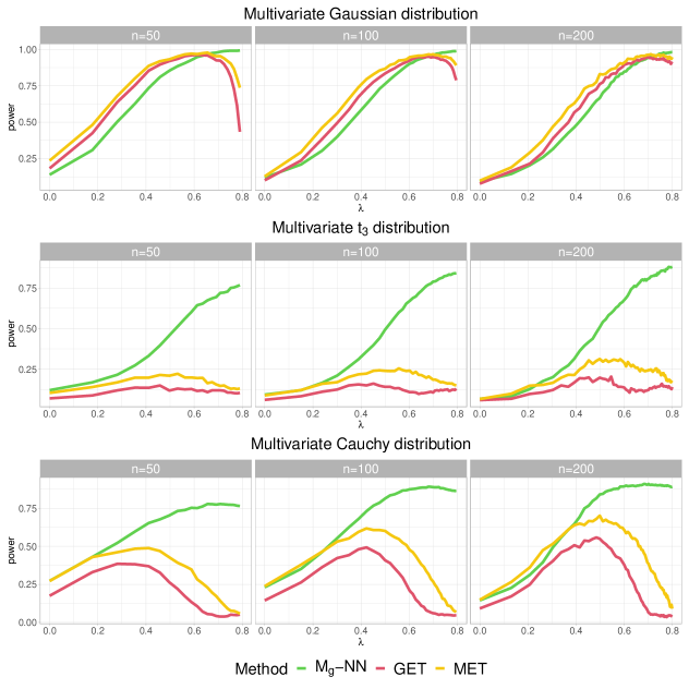
Figure 3: Empirical power of $\rm T_{g}$-NN, $\rm M_{g}$-NN, GET, and MET over $1000$ times of repetitions under each setting.

IV-B Performance comparison

We compare RING-CPD to GET and MET on $k$-MST ($k=[n^{0.5}]$), the graph-based method on the shortest Hamiltonian path [24] (SWR), the method based on Fréchet means and variances [49] (DM). We also compare three interpoint distance-based methods, the widely used distance-based method E-Divisive (ED) [21] implemented in the R package ecp, and the other two methods proposed recently by [22] and [29]. [22] proposed four statistics and we compare the statistic $C_{2N}$ that had a satisfactory performance in most of their simulation settings. [29] proposed three statistics, which perform well for location change, scale change, and general change, respectively. Here we compare with their statistic $S_{3}$, which they concluded to have relatively robust performance across various alternatives. For fairness, the $p$-values of all these methods are approximated by $1,000$ random permutations.

We set $n=200$ and the change-point $\tau=[n/3]$ and consider the dimension of the distributions $d=200,500,1000$. Before the change-point $y_{i}\sim F_{0}$ and after the change-point $y_{i}\sim F_{1}$. We consider both the empirical power and the detection accuracy estimated from $1000$ trails for each scenario. The empirical power is the ratio of the successful detection defined as $p$-value smaller than the nominal level $0.05$. The detection accuracy is provided in parentheses, which is the ratio of trials that the detected change-point is located in $[\tau-0.05n,\tau+0.05n]$ and the $p$-value smaller than $0.05$. We consider various settings that cover light-tailed, heavy-tailed, skewed, and mixture distributions for location, scale, and mixed alternatives. Specifically, we consider six settings for $F_{i}$, $i=0,1$:

1. the multivariate Gaussian distribution $N_{d}(\bm{\mu}_{i},\bm{\Sigma}_{i})$;

2. the multivariate $t_{5}$ distribution $t_{5}(\bm{\mu}_{i},\bm{\Sigma}_{i})$;

3. the multivariate Cauchy distribution ${\rm Cauchy}(\bm{\mu}_{i},\bm{\Sigma}_{i})$;

4. the multivariate $\chi_{5}^{2}$ distribution $\chi_{5}^{2}(\bm{\mu}_{i},\bm{\Sigma}_{i})$ (generated as $\bm{\Sigma}_{i}^{\frac{1}{2}}(X-5\mathbf{1}_{d}+\bm{\mu}_{i})$ where the $d$ components of $X$ are i.i.d. $\chi_{5}^{2}$);

5. the Gaussian mixture distribution $WN_{d}(\bm{\mu}_{i},\bm{\Sigma}_{i})+(1-W)N_{d}(-\bm{\mu}_{i},\bm{\Sigma}_{i})$ with $W\sim{\rm Bernoulli}(0.5)$;

6. the multivariate normal distribution with $t_{7}$ outliers $WN_{d}(\bm{\mu}_{i},\bm{\Sigma}_{i})+(1-W)t_{7}\big{(}\bm{\mu}_{i},\bm{\Sigma}_{i})$ with $W\sim{\rm Bernoulli}(0.9)$.

We set $\bm{\mu}_{0}=\mathbf{0}_{d}$ for $F_{0}$ and $\bm{\mu}_{1}=\delta\mathbf{1}_{d}$ for $F_{1}$, where $\delta$ is different for different settings. For each setting, we consider five different changes:

1. location ($\delta\neq 0$ and $\bm{\Sigma}_{1}=\bm{\Sigma}_{0}$);

2. simple scale ($\delta=0$ and $\bm{\Sigma}_{1}=(1+\sigma)^{2}\bm{\Sigma}_{0}$);

3. complex scale ($\delta=0$ and $\bm{\Sigma}_{1}\neq\bm{\Sigma}_{0}$);

4. location and simple scale mixed ($\delta\neq 0$ and $\bm{\Sigma}_{1}=(1+\sigma)^{2}\bm{\Sigma}_{0}$);

5. location and complex scale mixed ($\delta\neq 0$ and $\bm{\Sigma}_{1}\neq\bm{\Sigma}_{0}$).

The choice of $\delta$, $\sigma$, and $\bm{\Sigma}_{i}$, $i=1,2$ are specified differently for the settings and alternatives, summarized in Table II, where the changes in signal are set so that the best test has moderate power to be comparable. Here for Setting IV, the covariance matrices $\mathbf{A}_{i}=\mathbf{V}\mathbf{B}_{i}\mathbf{V}$, for $i=0,1,2$, where $\mathbf{V}$ is a diagonal matrix with the diagonal elements sampled independently from ${\rm U}(1,3)$, $\mathbf{B}_{i}={\rm diag}(\mathbf{B}_{i1},\ldots,\mathbf{B}_{i\frac{d}{10}})$ is a block-diagonal correlation matrix. Each diagonal block $\mathbf{B}_{ij}$ is a $10\times 10$ matrix with diagonal entries being $1$ and off-diagonal entries equal to $\rho_{ij}\sim{\rm U}(a_{j},b_{j})$ independently. We set $a_{0}=0,b_{0}=0.5$, $a_{1}=0.3,b_{1}=0.8$ and $a_{3}=0.2,b_{3}=0.7$. Each configuration is repeated $1,000$ times. We present the results of Settings I-III in Table III, and the results of Settings IV-VI in Table IV. Under each setting, the largest value and those larger than $95\%$ of the largest value are highlighted in bold.

TABLE II: The specific changes for different settings and alternatives.

		Alternative
Setting	$H_{0}$	(a)	(b)	(c)	(d)		(e)
	$\bm{\Sigma}_{0}$	$\delta$	$\sigma$	$\bm{\Sigma}_{1}$	$\delta$	$\sigma$	$\delta$	$\bm{\Sigma}_{1}$
(I)	$\bm{\Sigma}(0.6)$	$\frac{2\log d}{5\sqrt{d}}$	$\sqrt{\frac{\log d}{16d}}$	$\bm{\Sigma}(0.16)$	$\frac{\log d}{10\sqrt{d}}$	$\sqrt{\frac{\log d}{16d}}$	$\sqrt{\frac{\log d}{4d}}$	$\bm{\Sigma}(0.3)$
(II)	$\bm{\Sigma}(0.6)$	$\frac{5\log d}{4\sqrt{d}}$	$\frac{3\log d}{10\sqrt{d}}$	$0.6\bm{\Sigma}(0.1)$	$\frac{\log d}{3\sqrt{d}}$	$\frac{3\log d}{10\sqrt{d}}$	$\frac{\log d}{2\sqrt{d}}$	$\bm{\Sigma}(0.8)$
(III)	$\bm{\Sigma}(0.4)$	$\frac{11\log d}{20\sqrt{d}}$	$\frac{6\log d}{5d^{2/5}}$	$\bm{\Sigma}(0.85)$	$\frac{6\log d}{25d^{2/5}}$	$\sqrt{\frac{\log d}{25d}}$	$\frac{6\log d}{25d^{2/5}}$	$\bm{\Sigma}(0.6)$
(IV)	$\mathbf{A}_{0}$	$\frac{5\log d}{2\sqrt{d}}$	$\frac{9}{10\sqrt{d}}$	$\mathbf{A}_{1}$	$\sqrt{\frac{49\log d}{16d}}$	$\frac{3}{4\sqrt{d}}$	$\sqrt{\frac{49\log d}{16d}}$	$\mathbf{A}_{2}$
(V)	$\mathbf{I}_{d}$	$\frac{3}{5\log d}$	$\sqrt{\frac{\log d}{25d}}$	$\bm{\Sigma}(0.55)$	$\frac{3}{10\log d}$	$\sqrt{\frac{\log d}{25d}}$	$\frac{3}{10\log d}$	$\bm{\Sigma}(0.48)$
(VI)	$\bm{\Sigma}(0.5)$	$\frac{7\log d}{20\sqrt{d}}$	$\frac{\log d}{5\sqrt{d}}$	$\bm{\Sigma}(0.1)$	$\frac{\log d}{5\sqrt{d}}$	$\frac{\log d}{5\sqrt{d}}$	$\frac{\log d}{5\sqrt{d}}$	$\bm{\Sigma}(0.15)$

TABLE III: The empirical power (detection accuracy) in percent under Settings I-III.

	Setting I (Gaussian)			Setting II ($t_{5}$)			Setting III (Cauchy)
$d$	200	500	1000	200	500	1000	200	500	1000
	(a) Location change
$\rm M_{g}$-NN	76(58)	67(49)	59(40)	89(71)	79(59)	67(49)	99(88)	91(78)	72(55)
GET	63(46)	52(36)	40(25)	68(48)	41(26)	20(12)	85(72)	54(40)	28(17)
MET	68(50)	58(39)	46(30)	75(52)	50(32)	31(18)	90(75)	67(50)	44(26)
SWR	21(8)	18(6)	16(4)	19(6)	19(6)	15(4)	44(23)	40(18)	32(15)
DM	7(0)	6(0)	7(0)	6(0)	5(0)	4(0)	5(0)	4(0)	5(0)
ED	97(85)	96(83)	95(80)	73(57)	28(19)	12(4)	6(1)	5(0)	4(1)
$C_{2N}$	95(81)	93(81)	90(75)	53(34)	19(7)	8(2)	5(0)	5(0)	6(0)
$S_{3}$	5(1)	5(1)	6(0)	6(0)	5(0)	4(0)	5(0)	4(0)	5(0)
	(b) Simple scale change
$\rm M_{g}$-NN	65(38)	74(46)	80(51)	99(78)	94(68)	82(47)	98(70)	90(56)	81(46)
GET	61(33)	71(40)	74(44)	99(75)	86(56)	69(35)	97(68)	83(46)	63(32)
MET	63(36)	72(42)	76(47)	99(76)	91(63)	76(42)	98(68)	90(56)	77(43)
SWR	5(0)	5(0)	5(0)	33(14)	19(7)	13(3)	23(10)	20(5)	12(3)
DM	63(36)	50(21)	32(4)	72(47)	57(34)	43(24)	4(0)	4(0)	4(0)
ED	5(2)	6(1)	6(1)	98(78)	93(69)	83(56)	30(12)	19(8)	18(6)
$C_{2N}$	73(41)	84(53)	88(57)	73(42)	66(27)	54(11)	5(0)	5(0)	4(0)
$S_{3}$	83(54)	90(64)	92(67)	66(42)	49(28)	37(19)	4(0)	4(0)	4(0)
	(c) Complex scale change
$\rm M_{g}$-NN	96(73)	96(73)	95(72)	97(85)	85(61)	70(39)	95(80)	86(67)	76(55)
GET	84(63)	79(56)	79(56)	90(76)	35(2)	14(1)	96(84)	77(61)	54(38)
MET	78(48)	77(44)	76(46)	81(60)	37(10)	24(1)	94(78)	83(64)	70(50)
SWR	80(61)	84(64)	82(64)	96(84)	97(84)	96(83)	99(92)	98(88)	96(84)
DM	8(0)	6(0)	7(0)	70(46)	70(43)	68(40)	5(0)	5(0)	5(0)
ED	10(2)	10(2)	8(2)	95(72)	97(74)	95(75)	5(1)	6(0)	4(1)
$C_{2N}$	7(1)	7(1)	7(2)	74(40)	77(27)	75(15)	5(0)	4(0)	6(0)
$S_{3}$	8(1)	9(1)	8(1)	67(43)	67(41)	66(39)	5(0)	5(0)	5(0)
	(d) Location and simple scale mixed change
$\rm M_{g}$-NN	69(44)	73(46)	80(53)	69(48)	54(34)	37(21)	70(52)	60(43)	47(32)
GET	64(37)	67(39)	76(46)	53(34)	28(13)	12(4)	37(24)	23(14)	16(8)
MET	66(39)	71(43)	77(49)	51(30)	28(12)	16(5)	49(32)	34(20)	28(14)
SWR	5(0)	5(0)	5(0)	13(3)	12(3)	11(3)	20(7)	22(8)	19(6)
DM	66(40)	47(19)	32(5)	14(4)	8(2)	7(1)	5(0)	4(0)	4(0)
ED	9(2)	9(3)	8(2)	60(39)	32(18)	19(6)	6(1)	5(1)	4(1)
$C_{2N}$	77(44)	83(54)	89(61)	37(16)	16(4)	10(2)	6(0)	5(0)	5(0)
$S_{3}$	84(56)	88(63)	92(69)	11(2)	7(1)	6(1)	5(0)	4(0)	4(0)
	(e) Location and complex scale mixed change
$\rm M_{g}$-NN	84(56)	77(50)	74(45)	98(87)	96(84)	92(78)	78(59)	66(48)	54(39)
GET	68(45)	60(37)	54(31)	93(80)	80(64)	57(43)	49(34)	31(20)	20(11)
MET	65(38)	58(30)	53(27)	94(78)	85(67)	67(50)	60(43)	46(29)	34(18)
SWR	47(24)	42(22)	42(21)	65(41)	68(47)	64(43)	29(13)	29(13)	30(13)
DM	8(0)	8(0)	7(0)	3(0)	5(0)	5(0)	5(0)	4(0)	5(0)
ED	40(25)	33(17)	25(12)	90(72)	62(46)	22(15)	6(1)	4(0)	4(1)
$C_{2N}$	40(20)	28(11)	22(8)	61(40)	22(10)	10(3)	5(0)	5(0)	6(0)
$S_{3}$	6(0)	8(1)	6(0)	4(0)	5(0)	5(0)	5(0)	4(0)	5(0)

TABLE IV: The empirical power (detection accuracy) in percent under Settings IV-VI.

	Setting IV ($\chi_{5}^{2}$)			Setting V (Gaussian Mixture)			Setting VI (Gaussian outlier)
$d$	200	500	1000	200	500	1000	200	500	1000
	(a) Location change
$\rm M_{g}$-NN	74(56)	65(46)	54(37)	32(18)	42(27)	58(42)	61(44)	50(34)	42(24)
GET	60(43)	46(30)	33(21)	29(17)	39(25)	51(34)	44(30)	30(17)	21(9)
MET	64(47)	52(35)	39(25)	30(18)	41(28)	54(37)	48(33)	34(19)	27(13)
SWR	20(7)	18(6)	15(3)	20(6)	24(9)	31(13)	18(7)	15(4)	13(4)
DM	6(0)	5(0)	5(0)	7(0)	6(0)	7(0)	4(0)	6(0)	7(0)
ED	94(80)	93(79)	91(76)	6(1)	5(1)	6(1)	93(8)	90(73)	87(7)
$C_{2N}$	95(80)	92(78)	88(73)	87(53)	83(24)	84(11)	78(61)	44(26)	19(6)
$S_{3}$	5(1)	4(0)	6(1)	7(0)	6(0)	7(0)	4(0)	4(0)	6(0)
	(b) Simple scale change
$\rm M_{g}$-NN	90(64)	89(61)	86(58)	71(49)	81(58)	88(69)	84(61)	77(52)	70(47)
GET	85(57)	84(53)	80(51)	65(40)	76(51)	84(60)	87(61)	83(57)	75(51)
MET	88(61)	87(57)	83(54)	66(45)	76(55)	83(64)	85(59)	78(51)	72(44)
SWR	5(1)	6(0)	6(0)	5(0)	5(0)	5(1)	5(0)	5(0)	5(1)
DM	90(65)	82(52)	55(25)	6(0)	5(0)	5(0)	69(50)	59(40)	43(25)
ED	6(1)	8(2)	6(2)	5(1)	4(1)	5(1)	11(4)	13(4)	11(3)
$C_{2N}$	86(57)	91(63)	91(63)	6(1)	6(1)	6(0)	65(40)	56(31)	42(16)
$S_{3}$	93(68)	96(72)	96(72)	6(0)	5(0)	5(0)	53(38)	39(26)	24(14)
	(c) Complex scale change
$\rm M_{g}$-NN	74(49)	62(36)	58(33)	49(31)	42(28)	47(30)	72(50)	69(50)	66(47)
GET	57(40)	44(26)	37(20)	24(13)	18(9)	21(10)	44(28)	40(25)	37(24)
MET	52(29)	41(20)	36(15)	21(9)	15(6)	17(6)	45(27)	43(26)	44(25)
SWR	64(43)	63(43)	64 (42)	92(77)	92(79)	94(81)	58(36)	57(33)	57(34)
DM	4(0)	4(0)	4(0)	5(0)	5(0)	6(0)	5(1)	4(0)	4(0)
ED	8(1)	7(1)	8(1)	5(0)	5(1)	4(1)	8(1)	7(1)	7(0)
$C_{2N}$	3(0)	4(1)	5(0)	5(0)	5(0)	6(0)	5(0)	5(0)	6(0)
$S_{3}$	4(0)	4(0)	5(0)	5(0)	5(0)	6(0)	5(0)	5(0)	5(0)
	(d) Location and simple scale mixed change
$\rm M_{g}$-NN	70(42)	67(39)	63(38)	68(45)	81(56)	86(63)	86(62)	78(52)	74(47)
GET	66(37)	62(32)	58(31)	70(45)	81(56)	87(65)	93(71)	86(62)	80(60)
MET	66(39)	66(36)	60(34)	67(44)	79(57)	84(62)	88(64)	81(52)	75(50)
SWR	6(1)	5(0)	6(0)	7(1)	6(1)	7(1)	7(1)	8(2)	9(1)
DM	76(46)	57(27)	34(9)	7(0)	6(0)	6(0)	73(50)	59(37)	44(26)
ED	14(5)	10(3)	8(3)	5(1)	5(1)	4(1)	44(26)	38(22)	37(20)
$C_{2N}$	73(41)	77(44)	79(46)	52(22)	38(10)	38(5)	76(51)	57(32)	43(22)
$S_{3}$	82(54)	85(55)	85(56)	6(0)	6(0)	6(0)	55(38)	36(22)	24(14)
	(e) Location and complex scale mixed change
$\rm M_{g}$-NN	52(30)	41(23)	39(21)	42(25)	40(24)	45(29)	81(64)	76(59)	74(56)
GET	39(22)	25(12)	24(11)	19(9)	19(7)	20(10)	58(42)	49(32)	43(28)
MET	37(16)	26(11)	25(10)	15(6)	16(5)	18(7)	60(41)	52(34)	48(30)
SWR	42(22)	40(21)	40(19)	74(53)	76(54)	79(60)	56(33)	53(32)	50(29)
DM	4(0)	4(0)	5(0)	5(0)	5(0)	5(0)	4(0)	5(0)	4(0)
ED	10(2)	7(1)	7(1)	4(0)	5(1)	6(1)	43(25)	34(19)	28(14)
$C_{2N}$	8(2)	6(1)	5(0)	8(1)	9(1)	11(1)	20(9)	11(2)	4(0)
$S_{3}$	4(0)	4(0)	4(0)	5(0)	5(0)	5(0)	4(0)	6(0)	4(0)

For the multivariate $t_{5}$ and Cauchy distributions, $\rm M_{g}$-NN shows the highest power under the alternatives (a), (b), (d), and (e). SWR performs the best for the complex scale alternative (c), followed immediately by $\rm M_{g}$-NN, while GET and MET also have moderate power. On the contrary, DM, ED, $C_{2N}$ and $S_{3}$ fail for most of the alternatives under the multivariate $t_{5}$ and Cauchy distributions with the power close to the nominal level. It shows that $\rm M_{g}$-NN is robust to heavy-tailed distributions, while other methods such as $C_{2N}$ and $S_{3}$ are not.

From Table IV, we see that ED and $C_{2N}$ perform the best for the location alternative (a) under the multivariate $\chi_{5}^{2}$ distribution, while $\rm M_{g}$-NN performs the second best and $S_{3}$ has no power. For the scale alternative (b), $S_{3}$ exhibits the highest power, and $\rm M_{g}$-NN also performs well. In addition, under the same distribution, $\rm M_{g}$-NN and SWR outperform other methods for alternatives (c) and (e). However, SWR is powerless for alternative (d) while $\rm M_{g}$-NN shows good performance.

For the Gaussian mixture distribution, $C_{2N}$ has the highest power for the location alternative (a), while $\rm M_{g}$-NN is the second best. For alternatives (b) and (d), $\rm M_{g}$-NN has the best performance, together with GET and MET, while all other methods have unsatisfactory performance. For alternatives (c) and (e), SWR achieves the highest power, while $\rm M_{g}$-NN is also good with performance better than other methods.

For the multivariate normal distribution with $t_{7}$ outliers, ED is the best for the location alternative, while for $d=1000$, it is outperformed by $\rm M_{g}$-NN in the detection accuracy. For other alternatives, $\rm M_{g}$-NN almost dominates other methods, followed by GET and MET. It shows that $\rm M_{g}$-NN is robust to outliers.

In summary, the distance-based methods ED, $C_{2N}$, and $S_{3}$, as well as DM, are powerful for the light-tailed distribution. Specifically, ED exhibits superior power for the location alternative, $S_{3}$ and DM are more powerful for the simple scale alternative, while $C_{2N}$ covers both the location and the scale alternatives. Nevertheless, these methods suffer from outliers and are less powerful for heavy-tailed distributions. On the contrary, the graph-based methods GET and MET are less sensitive to outliers and show good performance for the complex scale alternative. The problem with these methods is that they use less information than distance-based methods, thus suffering from the lack of power for light-tailed distribution and the location alternative. In particular, SWR uses the least information compared to GET and MET, so it has almost no power in many settings and alternatives when other methods attain moderate power. On the other hand, $\rm M_{g}$-NN possesses good power for light-tailed distributions and shows robustness for heavy-tailed distributions.

V Real data examples

V-A Seizure detection from functional connectivity networks

We illustrate RING-CPD for identifying epileptic seizures, which over two million Americans are suffering from [50]. As a promising therapy, responsive neurostimulation requires automated algorithms to detect seizures as early as possible. Besides, to identify seizures, physicians have to review abundant electro-encephalogram (EEG) recordings, which in some patients may be quite subtle. Hence, it is important to develop methods with low false positive and false negative rates to detect seizures from the EEG recordings. We use the “Detect seizures in intracranial EEG (iEEG) recordings” database by the UPenn and Mayo Clinic (https://www.kaggle.com/c/seizure-detection) , which consists of the EEG recordings of $12$ subjects (eight patients and four dogs). For each subject, both the normal brain activity and the seizure activity are recorded multiple times, which are one-second clips with various channels (from $16$ to $72$), reducing to a multivariate stream of iEEGs. Following the preprocessing procedure of [3], we represent the iEEG data as functional connectivity networks using Pearson correlation in the high-gamma band ($70$-$100$Hz) [51]. Functional connectivity networks are weighted graphs, where the vertexes are the electrodes, and the weights of edges correspond to the coupling strength of the vertexes. An illustration of the networks is in Figure 4. The sample sizes of the $12$ subjects are also different, and the true change-point $\tau$’s are also known - before the change-point, the networks are from the seizure period, while after the change-point, the networks are from the normal brain activity, so we have the ground truth. We use the Frobenius norm to measure the distance between the observations represented by the weighted adjacency graphs.

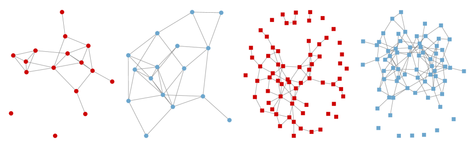
Figure 4: The functional connectivity networks of a dog (circle) and a human (square) during the period of the seizure (red) and the normal period (blue). The networks are drawn by only keeping the edges with weights larger than $0.2$.

We do not include SWR in the comparison here since SWR does not perform well in the simulation studies and is time-consuming. For $C_{2N}$, since it does well under some simulation settings, we try to include it in the comparison. However, it is not only time-consuming but also memory-consuming (e.g., it requires at least $17$Gb size of memory when $n=1320$); we are only able to run it for $n\leq 600$, thus only showing its result for Dog $1$, and Patients $1$ and $4$. Since the sample size of each subject is large enough, we use the asymptotic $p$-value approximation for $\rm M_{g}$-NN and MET. We omit the result of GET since it performs similarly to MET but its $p$-value approximation is not as exact as MET. For DM, ED, and $S_{3}$, we still use $1,000$ random permutations to obtain the $p$-values. The results are summarized in Table V, where the absolute difference between the true change-point and the detected change-point $|\hat{\tau}-\tau|$ is reported. The $p$-values are not reported as they are smaller than $0.01$ for all methods and subjects. Our method achieves the same detection error as MET, which is very small for all subjects. ED also performs well, but with a slightly large error for Patient $4$. Although DM and $S_{3}$ achieve small errors for most subjects, they attain large detection errors for Patients $3$ and $4$. The performance of $C_{2N}$ is not robust in that it shows a large detection error for Patient $4$.

TABLE V: The absolute difference between the true change-point and the detected change-point ($|\hat{\tau}-\tau|$). The $p$-values of all methods for all subjects are smaller than $0.01$.

Subject	$n$	$\tau$	$\rm M_{g}$-NN	MET	DM	ED	$C_{2N}$	$S_{3}$
Dog 1	596	178	0	0	0	1	0	0
Dog 2	1320	172	4	4	1	3	-	1
Dog 3	5240	480	0	0	1	1	-	1
Dog 4	3047	257	3	3	3	2	-	3
Patient 1	174	70	1	1	1	0	7	1
Patient 2	3141	151	7	7	13	1	-	13
Patient 3	1041	327	0	0	162	1	-	162
Patient 4	210	20	0	0	67	11	137	67
Patient 5	2745	135	3	3	5	2	-	5
Patient 6	2997	225	0	0	0	1	-	0
Patient 7	3521	282	2	2	3	4	-	3
Patient 8	1890	180	0	0	0	1	-	0

V-B Changed interval detection for New York taxi data

We illustrate our methods for changed interval detection in studying travel pattern changes around New York Central Park. We use the yellow taxi trip records for the year $2014$ from the NYC Taxi and Limousine Commission (TLC) website ( https://www1.nyc.gov/site/tlc/about/tlc-trip-record-data.page), which contains the city’s taxi pickup and drop-off times and locations (longitude and latitude coordinates). We set the latitude range of New York Central Park as $40.76$ to $40.81$ and the longitude range as $-74.10$ to $-73.60$. The boundary of New York City is set as $40.50$ to $40.95$ in latitude and $-74.10$ to $-73.60$. We only consider those trips that began with a pickup in New York City and ended with a drop-off in New York Central Park. We use the two-dimensional kernel density estimation with the bivariate normal kernel and $50$ grid points in each direction to represent the trips of each day in New York City, as illustrated by Figure 5 on two random days. We use the Frobenius norm to construct the similarity graphs in the subsequent analysis. The $p$-values of all methods are obtained through $1000$ random permutations.

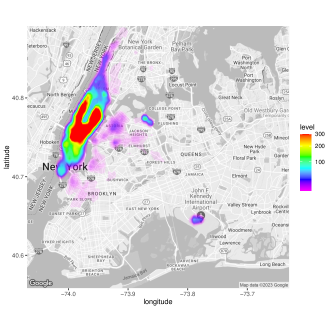
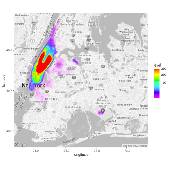
Figure 5: Density heatmap of taxi pick-ups for dates 01/01 and 02/01 in year 2014.

We first compare RING-CPD with GET and MET. We set $n_{0}=\max\{5,[0.05n]\}$ and $n_{1}=n-n_{0}$ and the nominal level as $0.01$. All methods detect the same changed interval $06/19$-$08/31$ with $p$-values $<0.001$, which almost overlaps totally with the summer break. Besides, $06/19$ is Juneteenth and $09/01$ is Labor Day.

Since there may be multiple changed intervals, we apply the methods recursively. Specifically, we apply the methods to the three segments divided by the detected changed interval. For the period of $01/01$-$06/18$, all methods detect the changed interval $03/18$-$03/28$ with $p$-value $<0.001$, which is around the spring break of most American universities, while $3/17$ is St. Patrick’s Day. For the period of $06/19$-$08/31$, no method can reject the null hypothesis at the $0.01$ significance level. For the period of $09/01$-$12/31$, $\rm M_{g}$-NN, GET, and MET report the changed interval starting at $09/01$, $09/03$, and $09/02$ respectively and all ending at $11/12$ with $p$-values $<0.001$. This is the changed interval of the Fall Semester till Veterans Day ($11/11$).

We further apply these methods to the segments divided by themselves longer than $40$ days. The only detected changed interval is $01/27$-$01/31$ reported by $\rm M_{g}$-NN with $p$-value $0.01$ in the segment $01/01$-$03/17$, which is around the Lunar New Year ($01/31/2014$). It is worth noting that for the period of $11/13$-$12/31$, all methods report the changed interval that covers Christmas, while $\rm M_{g}$-NN yields a small $p$-value $0.02$ and other methods report $p$-values larger than $0.05$. The results are summarized in Table VI.

TABLE VI: The detected changed intervals and corresponding $p$-values of $\rm M_{g}$-NN, GET and MET for the NYC taxi data.

Time period	$\rm M_{g}$-NN	GET	MET	Nearby Events
$01/01$-$12/31$	06/19-08/31			Summer break
$p$-value	$<0.001$
$01/01$-$06/18$	03/18-03/28			Spring break/St. Patrick’s Day
$p$-value	$<0.001$
$06/19$-$08/31$	$06/23$-$06/27$	$07/17$-$08/29$	$06/23$-$06/27$	-
$p$-value	$0.048$	$0.196$	$0.223$
$09/01$-$12/31$	09/01-11/12	09/03-11/12	09/02-11/12	Fall Semester (till Veterans Day)
$p$-value	$<0.001$
$01/01$-$03/17$	01/27-01/31	$02/19$-$03/13$	$02/19$-$03/13$	Lunar New Year
$p$-value	$0.01$	$0.051$	$0.263$
$03/29$-$06/18$	$04/04$-$06/15$	$04/23$-$05/22$	$04/23$-$05/23$	-
$p$-value	$0.094$	$0.366$	$0.333$
$09/01(03,02)$-$11/12$	$09/02$-$09/11$	$09/03$-$09/11$	$09/02$-$09/12$	-
$p$-value	$0.014$	$0.073$	$0.028$
$11/13$-$12/31$	$12/22$-$12/30$	$12/20$-$12/30$	$12/20$-$12/30$	-
$p$-value	$0.020$	$0.067$	$0.059$
$02/01$-$03/17$	$03/03$-$03/07$			-
$p$-value	$0.263$

We also apply other methods to the dataset. Since both ED and $S_{3}$ can detect multiple change points, we apply them directly to the whole sequence $01/01$-$12/31$. We also include $C_{2N}$. Although $C_{2N}$ is not designed for multiple change-point detections, we adopt the same binary segmentation procedure $S_{3}$ used [29]. As summarized in Table VII, ED detects two change-points $06/20$ and $09/02$ both with $p$-values $0.001$. $S_{3}$ only detects one change-point $06/20$ with $p$-value $0.003$. $C_{2N}$ detects two change-points, which are $06/19$ and $09/14$, with $p$-values $<0.001$ and $0.004$. They all miss some important change-points shown in Table VI.

TABLE VII: The detected change-points and corresponding $p$-values of ED, $S_{3}$ and $C_{2N}$ for the NYC taxi data.

Method	ED		$S_{3}$	$C_{2N}$
CP	$06/20$	$09/02$	$06/20$	$06/19$	$09/14$
$p$-value	$0.001$	$0.001$	$0.003$	$<0.001$	$0.004$

VI Discussion

VI-A Kernel and Distance IN Graph CPD

The approach proposed in this paper can also be extended to weights other than ranks in weighting the edges in the similarity graph. For example, we could incorporate kernel value or distance directly to have Kernel IN Graph Change-Point Detection (KING-CPD) and Distance IN Graph Change-Point Detection (DING-CPD) methods. Specifically, we can use the kernel values or (negative) pairwise distances to weight the similarity graph, and the asymptotic property still holds under mild conditions. Let

$$K_{ij}=K(y_{i},y_{j})\mathbbm{1}\big{(}(i,j)\in G_{k}\big{)}\,,$$

where $K$ is a kernel function or a negative distance function, for example, the Gaussian kernel $K(y_{i},y_{j})=\exp\big{(}-\|y_{i}-y_{j}\|^{2}/(2\sigma^{2})\big{)}$ with the kernel bandwidth $\sigma$ or $K(y_{i},y_{j})$ simply the negative $l_{1}$ distance $K(y_{i},y_{j})=-\|y_{i}-y_{j}\|_{1}$, and $G_{k}$ is a similarity graph such as the $k$-NNG or the $k$-MST. We require Condition (7) $\max_{i,j}K_{ij}=o\big{(}n^{2}r_{d}^{2}\big{)}$, which essentially states that there is no element of $K_{ij}$ dominates others.

Theorem 3

Replacing $R_{ij}$ by $K_{ij}$ in Conditions (1)-(6), and the definition of $Z_{\mathrm{diff}}$ and $Z_{w}$, then under Conditions (1)-(6) and (7), we have

1. $\big{\{}Z_{\mathrm{diff}}(\lfloor nu\rfloor):0<u<1\big{\}}$ and $\big{\{}Z_{w}(\lfloor nu\rfloor):0<u<1\big{\}}$ converge to independent Gaussian processes in finite-dimensional distributions, which we denote as $\big{\{}Z_{\mathrm{diff}}^{*}(u):0<u<1\big{\}}$ and $\big{\{}Z_{w}^{*}(u):0<u<1\big{\}}$, respectively.

2. $\big{\{}Z_{\mathrm{diff}}(\lfloor nu\rfloor,\lfloor nv\rfloor):0<u<v<1\big{\}}$ and $\big{\{}Z_{w}(\lfloor nu\rfloor,\lfloor nv\rfloor):0<u<v<1\big{\}}$ converge to independent two-dimension Gaussian random fields in finite-dimensional distributions, which we denote as $\big{\{}Z_{\mathrm{diff}}^{*}(u,v):0<u<v<1\big{\}}$ and $\big{\{}Z_{w}^{*}(u,v):0<u<v<1\big{\}}$, respectively.

Besides, Theorem 2 also holds by replacing $R_{ij}$ by $K_{ij}$.

The proof of Theorem 3 follows straightforwardly from the proof of Theorems 1 and 2, thus omitted here.

VI-B Computational efficiency

Another useful property of RING-CPD is the potential computational efficiency by avoiding computing the pairwise distance of the $n$ observations, which has a computational complexity of $O(dn^{2})$ for $d$-dimensional data. Specifically, if the approximate $k$-NNG [52] is used for RING-CPD, the computational complexity is $O\big{(}dn(\log n+k\log d)+nk^{2}\big{)}$, which is usually faster than $O(dn^{2})$ when $k$ is small. A detailed discussion of the procedure and time complexity can be found in [28].

References

- [1] E. S. Page, “Continuous inspection schemes,” Biometrika, vol. 41, no. 1/2, pp. 100–115, 1954.
- [2] I. Barnett and J.-P. Onnela, “Change point detection in correlation networks,” Scientific reports, vol. 6, no. 1, pp. 1–11, 2016.
- [3] D. Zambon, C. Alippi, and L. Livi, “Change-point methods on a sequence of graphs,” IEEE Transactions on Signal Processing, vol. 67, no. 24, pp. 6327–6341, 2019.
- [4] M. Staudacher, S. Telser, A. Amann, H. Hinterhuber, and M. Ritsch-Marte, “A new method for change-point detection developed for on-line analysis of the heart beat variability during sleep,” Physica A: Statistical Mechanics and its Applications, vol. 349, no. 3-4, pp. 582–596, 2005.
- [5] R. Malladi, G. P. Kalamangalam, and B. Aazhang, “Online bayesian change point detection algorithms for segmentation of epileptic activity,” in 2013 Asilomar conference on signals, systems and computers. IEEE, 2013, pp. 1833–1837.
- [6] G. Kossinets and D. J. Watts, “Empirical analysis of an evolving social network,” science, vol. 311, no. 5757, pp. 88–90, 2006.
- [7] N. Eagle, A. S. Pentland, and D. Lazer, “Inferring friendship network structure by using mobile phone data,” Proceedings of the national academy of sciences, vol. 106, no. 36, pp. 15 274–15 278, 2009.
- [8] L. Peel and A. Clauset, “Detecting change points in the large-scale structure of evolving networks,” in Twenty-Ninth AAAI Conference on Artificial Intelligence, 2015.
- [9] J. Bai and P. Perron, “Estimating and testing linear models with multiple structural changes,” Econometrica, pp. 47–78, 1998.
- [10] M. Talih and N. Hengartner, “Structural learning with time-varying components: tracking the cross-section of financial time series,” Journal of the Royal Statistical Society: Series B (Statistical Methodology), vol. 67, no. 3, pp. 321–341, 2005.
- [11] M. Srivastava and K. J. Worsley, “Likelihood ratio tests for a change in the multivariate normal mean,” Journal of the American Statistical Association, vol. 81, no. 393, pp. 199–204, 1986.
- [12] N. R. Zhang, D. O. Siegmund, H. Ji, and J. Z. Li, “Detecting simultaneous changepoints in multiple sequences,” Biometrika, vol. 97, no. 3, pp. 631–645, 2010.
- [13] D. Siegmund, B. Yakir, and N. R. Zhang, “Detecting simultaneous variant intervals in aligned sequences,” The Annals of Applied Statistics, vol. 5, no. 2A, pp. 645–668, 2011.
- [14] J. Chen and A. K. Gupta, Parametric statistical change point analysis: with applications to genetics, medicine, and finance. Springer, 2012.
- [15] G. Wang, C. Zou, and G. Yin, “Change-point detection in multinomial data with a large number of categories,” The Annals of Statistics, vol. 46, no. 5, pp. 2020–2044, 2018.
- [16] F. Desobry, M. Davy, and C. Doncarli, “An online kernel change detection algorithm,” IEEE Transactions on Signal Processing, vol. 53, no. 8, pp. 2961–2974, 2005.
- [17] S. Li, Y. Xie, H. Dai, and L. Song, “M-statistic for kernel change-point detection,” Advances in Neural Information Processing Systems, vol. 28, 2015.
- [18] D. Garreau and S. Arlot, “Consistent change-point detection with kernels,” Electronic Journal of Statistics, vol. 12, no. 2, pp. 4440–4486, 2018.
- [19] S. Arlot, A. Celisse, and Z. Harchaoui, “A kernel multiple change-point algorithm via model selection,” Journal of machine learning research, vol. 20, no. 162, 2019.
- [20] W.-C. Chang, C.-L. Li, Y. Yang, and B. Póczos, “Kernel change-point detection with auxiliary deep generative models,” arXiv preprint arXiv:1901.06077, 2019.
- [21] D. S. Matteson and N. A. James, “A nonparametric approach for multiple change point analysis of multivariate data,” Journal of the American Statistical Association, vol. 109, no. 505, pp. 334–345, 2014.
- [22] J. Li, “Asymptotic distribution-free change-point detection based on interpoint distances for high-dimensional data,” Journal of Nonparametric Statistics, vol. 32, no. 1, pp. 157–184, 2020.
- [23] H. Chen and N. Zhang, “Graph-based change-point detection,” The Annals of Statistics, vol. 43, no. 1, pp. 139–176, 2015.
- [24] X. Shi, Y. Wu, and C. R. Rao, “Consistent and powerful graph-based change-point test for high-dimensional data,” Proceedings of the National Academy of Sciences, vol. 114, no. 15, pp. 3873–3878, 2017.
- [25] L. Chu and H. Chen, “Asymptotic distribution-free change-point detection for multivariate and non-euclidean data,” The Annals of Statistics, vol. 47, no. 1, pp. 382–414, 2019.
- [26] H. Chen, “Change-point detection for multivariate and non-euclidean data with local dependency,” arXiv preprint arXiv:1903.01598, 2019.
- [27] H. Song and H. Chen, “Asymptotic distribution-free change-point detection for data with repeated observations,” arXiv preprint arXiv:2006.10305, 2020.
- [28] Y.-W. Liu and H. Chen, “A fast and efficient change-point detection framework for modern data,” arXiv preprint arXiv:2006.13450, 2020.
- [29] L. Nie and D. L. Nicolae, “Weighted-graph-based change point detection,” arXiv preprint arXiv:2103.02680, 2021.
- [30] H. Chen and J. H. Friedman, “A new graph-based two-sample test for multivariate and object data,” Journal of the American statistical association, vol. 112, no. 517, pp. 397–409, 2017.
- [31] G. K. Bhattacharyya and R. A. Johnson, “Nonparametric tests for shift at an unknown time point,” The Annals of Mathematical Statistics, pp. 1731–1743, 1968.
- [32] B. Darkhovskh, “A nonparametric method for the a posteriori detection of the “disorder” time of a sequence of independent random variables,” Theory of Probability & Its Applications, vol. 21, no. 1, pp. 178–183, 1976.
- [33] A. N. Pettitt, “A non-parametric approach to the change-point problem,” Journal of the Royal Statistical Society: Series C (Applied Statistics), vol. 28, no. 2, pp. 126–135, 1979.
- [34] E. Schechtman, “A nonparametric test for detecting changes in location,” Communications in Statistics-Theory and Methods, vol. 11, no. 13, pp. 1475–1482, 1982.
- [35] F. Lombard, “Rank tests for changepoint problems,” Biometrika, vol. 74, no. 3, pp. 615–624, 1987.
- [36] ——, “Asymptotic distributions of rank statistics in the change-point problem,” South African Statistical Journal, vol. 17, no. 1, pp. 83–105, 1983.
- [37] C. Gerstenberger, “Robust wilcoxon-type estimation of change-point location under short-range dependence,” Journal of Time Series Analysis, vol. 39, no. 1, pp. 90–104, 2018.
- [38] Y. Wang, Z. Wang, and X. Zi, “Rank-based multiple change-point detection,” Communications in Statistics-Theory and Methods, vol. 49, no. 14, pp. 3438–3454, 2020.
- [39] A. Lung-Yut-Fong, C. Lévy-Leduc, and O. Cappé, “Homogeneity and change-point detection tests for multivariate data using rank statistics,” Journal de la Société Française de Statistique, vol. 156, no. 4, pp. 133–162, 2015.
- [40] C. Zhang, N. Chen, and J. Wu, “Spatial rank-based high-dimensional monitoring through random projection,” Journal of Quality Technology, vol. 52, no. 2, pp. 111–127, 2020.
- [41] L. Shu, Y. Chen, W. Zhang, and X. Wang, “Spatial rank-based high-dimensional change point detection via random integration,” Journal of Multivariate Analysis, vol. 189, p. 104942, 2022.
- [42] S. Chenouri, A. Mozaffari, and G. Rice, “Robust multivariate change point analysis based on data depth,” Canadian Journal of Statistics, vol. 48, no. 3, pp. 417–446, 2020.
- [43] D. Zhou and H. Chen, “Rise: Rank in similarity graph edge-count two-sample test,” arXiv preprint arXiv:2011.06127, 2021.
- [44] Y. Zhang and H. Chen, “Graph-based multiple change-point detection,” arXiv preprint arXiv:2110.01170, 2021.
- [45] P. Fryzlewicz, “Wild binary segmentation for multiple change-point detection,” The Annals of Statistics, vol. 42, no. 6, pp. 2243–2281, 2014.
- [46] S. Kovács, H. Li, P. Bühlmann, and A. Munk, “Seeded binary segmentation: A general methodology for fast and optimal change point detection,” arXiv preprint arXiv:2002.06633, 2020.
- [47] J. H. Friedman and L. C. Rafsky, “Multivariate generalizations of the wald-wolfowitz and smirnov two-sample tests,” The Annals of Statistics, pp. 697–717, 1979.
- [48] D. Siegmund and B. Yakir, The statistics of gene mapping. Springer Science & Business Media, 2007.
- [49] P. Dubey and H.-G. Müller, “Fréchet change point detection,” 2020.
- [50] L. D. Iasemidis, “Epileptic seizure prediction and control,” IEEE Transactions on Biomedical Engineering, vol. 50, no. 5, pp. 549–558, 2003.
- [51] A. M. Bastos and J.-M. Schoffelen, “A tutorial review of functional connectivity analysis methods and their interpretational pitfalls,” Frontiers in systems neuroscience, vol. 9, p. 175, 2016.
- [52] A. Beygelzimer, S. Kakadet, J. Langford, S. Arya, D. Mount, and S. Li, “Fast nearest neighbor search algorithms and applications,” FNN: kd-tree fast k-nearest neighbor search algorithms, 2019.