Relaxed Gaussian Process Interpolation:
a Goal-Oriented Approach to Bayesian Optimization

Abstract

This work presents a new procedure for obtaining predictive distributions in the context of Gaussian process (GP) modeling, with a relaxation of the interpolation constraints outside some ranges of interest: the mean of the predictive distributions no longer necessarily interpolates the observed values when they are outside ranges of interest, but are simply constrained to remain outside. This method called relaxed Gaussian process (reGP) interpolation provides better predictive distributions in ranges of interest, especially in cases where a stationarity assumption for the GP model is not appropriate. It can be viewed as a goal-oriented method and becomes particularly interesting in Bayesian optimization, for example, for the minimization of an objective function, where good predictive distributions for low function values are important. When the expected improvement criterion and reGP are used for sequentially choosing evaluation points, the convergence of the resulting optimization algorithm is theoretically guaranteed (provided that the function to be optimized lies in the reproducing kernel Hilbert spaces attached to the known covariance of the underlying Gaussian process). Experiments indicate that using reGP instead of stationary GP models in Bayesian optimization is beneficial.

Keywords: Gaussian processes; Bayesian optimization; Expected improvement; Goal-oriented modeling; Reproducing kernel Hilbert spaces

1 Introduction

1.1 Context and Motivation

Gaussian process (GP) interpolation and regression (see, e.g., Stein, 1999; Rasmussen and Williams, 2006) is a very classical method for predicting an unknown function from data. It has found applications in active learning techniques, and notably in Bayesian optimization, a popular derivative-free global optimization technique for functions whose evaluations are time-consuming.

A GP model is defined by a mean and a covariance functions, which are generally selected from data within parametric families. The most popular models assume stationarity and rely on standard covariance functions such as the Matérn covariance. The assumption of stationarity yields models with relatively low-dimensional parameters. However, such a hypothesis can sometimes result in poor models when the function to be predicted has different scales of variation or different local regularities across the domain.

This is the case for instance in the motivating example given by Gramacy and Lee (2008), or in the even simpler toy minimization problem shown in Figure 1. The objective function in this example, which we shall call the Steep function, is smooth with an obvious global minimum around the point $x=8$. However, the variations around the minimum are overshadowed by some steep variations on the left. Figure 2 shows a stationary GP fit with $n=8$ points, where the parameters of the covariance function have been selected using maximum likelihood. Observe that the confidence bands are too large and that the conditional mean varies too much in the neighborhood of the global minimum, consistently with the stationary GP model that reflects the prior that our function oscillates around a mean value with a constant scale of variations. In this case, even if GP interpolation is consistent (Vazquez and Bect, 2010a), stationarity seems an unsatisfactory assumption for the Steep function. One expects Bayesian optimization techniques to be somehow inefficient on this problem with such a stationary model, whose posterior distributions are too pessimistic in the region of the minimum.

Nevertheless, the Steep function has the characteristics of an easy optimization problem: it has only two local minima, with the global minimum lying in a valley of significant volume. Consequently, a Bayesian optimization technique could be competitive if it relied on a model giving good predictions in regions where the function takes low values. In this work, we propose to explore goal-oriented GP modeling, where we want predictive models in regions of interest, even if it means being less predictive elsewhere.

Figure 1: Left: the Steep function. Right: same illustration with a restrained range on the $y$-axis. The variations on the left overshadow the global minimum on the right.

Figure 2: Left: GP fit on the Steep function. Right: same illustration with a restrained range on the $y$-axis. The squares represent the data. The red line represents the posterior mean $\mu_{n}$ given by the model and the gray envelopes represent the associated uncertainties.

1.2 Related Works

Going beyond the stationary hypothesis has been an active direction of research. With maybe a little bit of oversimplification, one can distinguish two categories of approaches that all use stationary Gaussian processes as a core building block: local models and transformation/composition of models.

1.2.1 Local Models

A first class of local models is obtained by considering partitions of the input domain with different GP models on each subset. Partitions can be built by splitting the domain along the coordinate axes. This is the case of the treed Gaussian process models proposed by Gramacy and Lee (2008), which combines a fully Bayesian framework and the use of RJ-MCMC techniques for the inference, or the trust-region method by Eriksson et al. (2019). Park and Apley (2018) also propose partition-based local models built by splitting the domain along principal component directions. In such techniques, there are parameters (often many of them) related to, e.g., the way the partitions evolve with the data, the size of the partitions, or how local Gaussian processes interact with each other.

A second class of local models is obtained by spatially weighting one or several GP models. Many schemes have been proposed, including methods based on partition of unity (Nott and Dunsmuir, 2002), weightings of covariance functions (Pronzato and Rendas, 2017; Rivoirard and Romary, 2011), and convolution techniques (see, e.g., Higdon, 1998; Gibbs, 1998; Higdon, 2002; Ver Hoef et al., 2004; Stein, 2005). Let us also mention data-driven aggregation techniques: composite Gaussian process models (Ba and Joseph, 2012), and mixture of experts techniques (see, e.g., Tresp, 2001; Rasmussen and Ghahramani, 2002; Meeds and Osindero, 2006; Yuan and Neubauer, 2009; Yang and Ma, 2011; Yuksel et al., 2012). In the latter framework, the weights are called gating functions and the estimation of the parameters and the inference are usually performed using EM, MCMC, or variational techniques. Weighting methods generally have parameters specifying weighting functions, with an increased need to watch for overfitting phenomena.

1.2.2 Transformation and Composition of Models

A first technique for composition of models consists in using a parametric transformation of a GP (Rychlik et al., 1997; Snelson et al., 2004).

Another route is to transform the input domain, using for instance a parametric density (Xiong et al., 2007), or other parametric transformations involving possible dimension reduction (Marmin et al., 2018). Bodin et al. (2020) proposed a framework that uses additional input variables, serving as nuisance parameters, to smooth out some badly behaved data. The practitioner has to specify a prior over the variance of the nuisance parameter and inference is based on MCMC.

Lázaro-Gredilla (2012) takes the step of choosing a GP prior on the output transform and resorts to variational inference techniques for inference. This type of idea can be viewed as an ancestor of deep Gaussian processes (see, e.g., Damianou and Lawrence, 2013; Dunlop et al., 2018; Hebbal et al., 2021; Jakkala, 2021; Bachoc and Lagnoux, 2021), which stack layers of linear combinations of GPs. The practitioner has to specify a network structure among other parameters and resort to variational inference.

Recently, Picheny et al. (2019) proposed another approach where prediction is made only from pairwise comparisons between data points, relying on the variational framework of ordinal GP regression proposed by Chu and Ghahramani (2005) for the inference.

1.3 Contributions and Outline

The brief review of the literature above reveals three types of shortcomings in methods that depart from the stationarity hypothesis: 1) they rely on advanced techniques for deriving predictive distributions; or 2) they require the practitioner to choose in advance some key parameters; or 3) they increase the number of parameters with an increased risk of overfitting.

This article suggests a method for building models targeting regions of interest specified through function values. The main objective is to obtain global models that exhibit good predictive distributions on a range of interest. In the case of a minimization problem, the range of interest would be the values below a threshold. Outside the range of interest, we accept that the model can be less predictive by relaxing the interpolation constraints. Such a model is presented in Figure 3: compared to the situation in Figure 2, the model is more predictive in the region where the Steep function takes low values, with expected benefits for the efficiency of Bayesian optimization.

Figure 3: Left: prediction of the Steep function with the proposed methodology (black line: relaxation threshold $t$; blue points: relaxed observations). Right: $\mu_{n}$ versus $f$ (with more observations for illustration purposes). The model interpolates the data below $t$. The blue points are relaxed observations.

This article provides three main contributions. First, we propose a class of goal-oriented GP-based models called relaxed Gaussian processes (reGP). Second, we give theoretical and empirical results justifying the method and its use for Bayesian optimization. Finally, to assess the predictivity of reGP, we adopt the formalism of scoring rules (Gneiting and Raftery, 2007) and propose the use of a goal-oriented scoring rule that we call truncated continuous ranked probability score (tCRPS), which is designed to assess the predictivity of a model in a range of interest.

The organization is as follows. Section 2 briefly recalls the formalism of Gaussian processes and Bayesian optimization (BO). Section 3 presents reGP and its theoretical properties. The tCRPS and its use for selecting regions of interest are then presented in Section 4. Section 5 presents a reGP-based Bayesian optimization algorithm called EGO-R, together with the convergence analysis of this algorithm and a numerical benchmark. Finally, Section 6 presents our conclusions and perspectives for future work.

2 Background and Notations

2.1 Gaussian Process Modeling

Consider a real-valued function $f:\mathds{X}\to\mathds{R}$, where $\mathds{X}\subseteq\mathds{R}^{d}$, and suppose we want to infer $f$ at a given $x\in\mathds{X}$ from evaluations of $f$ on a finite set of points $\underline{x}_{n}=(x_{1},\ldots,x_{n})\in\mathds{X}^{n}$, $n\geq 1$. A standard Bayesian approach to this problem consists in using a GP model $\xi\sim\mathop{\mathrm{GP}}\left(\mu,\,k\right)$ as a prior about $f$, where $\mu:\mathds{X}\to\mathds{R}$ is a mean function and $k:\mathds{X}\times\mathds{X}\to\mathds{R}$ is a covariance function, which is supposed to be strictly positive-definite in this article.

The posterior distribution of $\xi$ given $\underline{Z}_{n}=\left(\xi(x_{1}),\cdots,\xi(x_{n})\right)^{\mathsf{T}}$ is still a Gaussian process, whose mean and covariance functions are given by the standard kriging equations (Matheron, 1971). More precisely:

$$\xi\,|\,\underline{Z}_{n}\sim\mathop{\mathrm{GP}}\left(\mu_{n},\,k_{n}\right),$$ (1)

with

$$\mu_{n}(x)=\mu(x)+k\left(x,\,\underline{x}_{n}\right)K_{n}^{-1}\left(\underline{Z}_{n}-\mu(\underline{x}_{n})\right)$$ (2)

and

$$k_{n}(x,\,y)=k(x,\,y)-k\left(x,\,\underline{x}_{n}\right)K_{n}^{-1}k\left(y,\,\underline{x}_{n}\right)^{\mathsf{T}}\,,$$ (3)

and where $\mu(\underline{x}_{n})=\left(\mu(x_{1}),\dots,\mu(x_{n})\right)^{\mathsf{T}}$, $k\left(x,\,\underline{x}_{n}\right)=\left(k(x,\,x_{1}),\dots,k(x,\,x_{n})\right)$, and $K_{n}$ is the $n\times n$ matrix with entries $k(x_{i},\,x_{j})$. We shall also use the notation $\sigma_{n}^{2}(x)=k_{n}(x,\,x)$ for the posterior variance, a.k.a. the kriging variance, a.k.a. the squared power function, so that $\xi(x)\,|\,\underline{Z}_{n}\sim\mathcal{N}\left(\mu_{n}(x),\,\sigma_{n}^{2}(x)\right)$.

The functions $\mu$ and $k$ control the posterior distribution (1) and must be chosen carefully. The standard practice is to select them from data within a parametric family $\{\left(\mu_{\theta},k_{\theta}\right),\ \theta\in\Theta\}$. A common approach is to suppose stationarity for the GP, which means choosing a constant mean function $\mu\equiv c\in\mathds{R}$ and a stationary covariance function $k(x,y)=\sigma^{2}r(x-y)$, where $r:\mathds{R}^{d}\to\mathds{R}$ is a stationary correlation function.

A correlation function often recommended in the literature (Stein, 1999) is the (geometrically anisotropic) Matérn correlation function

$$r(h)=\frac{2^{1-\nu}}{\Gamma(\nu)}\left(\sqrt{2\nu}\lVert h\rVert_{\rho}\right)^{\nu}\mathcal{K}_{\nu}\left(\sqrt{2\nu}\lVert h\rVert_{\rho}\right)\,,\quad\lVert h\lVert_{\rho}^{2}=\sum_{j=1}^{d}\frac{h_{\left[j\right]}^{2}}{\rho_{j}^{2}}\,,$$ (4)

for $h=(h_{[1]},\,\ldots,\,h_{[d]})\in\mathds{R}^{d}$, and where $\Gamma$ is the Gamma function and $\mathcal{K}_{\nu}$ is the modified Bessel function of the second kind. The parameters to be selected in this case are $(\sigma^{2},\,\rho_{1},\,\ldots,\,\rho_{d},\,\nu)\in\left(0,\infty\right)^{d+2}$ with $\sigma^{2}$ the process variance, $\rho_{i}$ the range parameter along the $i$-th dimension, and $\nu$ a regularity parameter controlling the smoothness of the process. Two other standard covariance functions can be recovered for specific values of $\nu$: the exponential covariance function for $\nu=1/2$ and the squared-exponential covariance function for $\nu\to\infty$.

A variety of techniques for selecting the parameter $\theta$ have been proposed in the literature, but we can safely say that maximum likelihood estimation is the most popular and can be recommended in the case of interpolation (Petit et al., 2021). It simply consists in minimizing the negative log-likelihood

$$\mathcal{L}\left(\theta;\,\underline{Z}_{n}\right)=-\log\left(p\left(\underline{Z}_{n}\,\lvert\,\theta\right)\right)\propto\log\left(\det\left(K_{n}\right)\right)+(\underline{Z}_{n}-\mu(\underline{x}_{n}))^{\mathsf{T}}K_{n}^{-1}(\underline{Z}_{n}-\mu(\underline{x}_{n}))+\text{constant},$$ (5)

where $p$ stands for the probability density of $\underline{Z}_{n}$. Other methods for selecting the parameters include the restricted maximum likelihood method and leave-one-out strategies (see, e.g., Stein, 1999; Rasmussen and Williams, 2006).

2.2 Bayesian Optimization

The framework of GPs is well suited to the problem of sequential design of experiments, or active learning. In particular, for minimizing a real-valued function $f$ defined on a compact domain $\mathds{X}$, the Bayesian approach consists in choosing sequentially evaluation points $X_{1},\,X_{2},\,\ldots\in\mathds{X}$ using a GP model $\xi$ for $f$, which makes it to possible to build a sampling criterion that represents an expected information gain on the minimum of $f$ when an evaluation is made at a new point. One of the most popular sampling criterion (also called acquisition function) is the Expected Improvement (EI) (Mockus et al., 1978; Jones et al., 1998), which can be expressed as

$$\rho_{n}(x)=\mathsf{E}\left(\left(m_{n}-\xi(x)\right)_{+}\,\lvert\,\underline{Z}_{n}\right),$$ (6)

where $m_{n}=\min(\xi(x_{1}),\cdots,\xi(x_{n}))$. The EI criterion corresponds to the expectation of the excursion of $\xi$ below the minimum given $n$ observations, and can be written in closed form:

Proposition 1

(Jones et al., 1998; Vazquez and Bect, 2010b) The EI criterion may be written as $\rho_{n}(x)=\gamma\left(m_{n}-\mu_{n}(x),\,\sigma_{n}^{2}(x)\right)$ with

$$\gamma:(z,\,s)\in\mathds{R}\times\mathds{R}_{+}\mapsto\left\{\begin{array}[]{ll}\sqrt{s}\phi\left(\frac{z}{\sqrt{s}}\right)+z\Phi\left(\frac{z}{\sqrt{s}}\right)&\ \mathrm{if}\ s>0,\\ \max(z,0)&\ \mathrm{if}\ s=0,\end{array}\right.$$

where $\phi$ and $\Phi$ stand for the probability density and cumulative distribution functions of the standard Gaussian distribution. Moreover, the function $\gamma$ is continuous, verifies $\gamma(z,\,s)>0$ if $s>0$ and is non-decreasing with respect to $z$ and $s$ on $\mathds{R}\times\mathds{R}_{+}$.

When the EI criterion is used for optimization, that is, when the sequence of evaluation points $(X_{n})_{n>0}$ of $f$ is chosen using the rule

$$X_{n+1}=\operatorname*{arg\,max}_{x\in\mathds{X}}\rho_{n}(x)\,,$$

the resulting algorithm is generally called the Efficient Global Optimization (EGO) algorithm, as proposed by Jones et al. (1998). The EGO algorithm has known convergence properties (Vazquez and Bect, 2010b; Bull, 2011).

A variety of other sampling criteria for the minimization problem can be found in the literature (see, e.g., Frazier et al., 2008; Villemonteix et al., 2009; Srinivas et al., 2010; Vazquez and Bect, 2014), but we shall focus on the EI algorithm in this article.

2.3 Reproducing Kernel Hilbert Spaces

Reproducing kernel Hilbert spaces (RKHS, see e.g., Aronszajn, 1950; Berlinet and Thomas-Agnan, 2004) are Hilbert spaces of functions commonly used in the field of approximation theory (see, e.g., Wahba, 1990; Wendland, 2004). A Hilbert space $\mathcal{H}(\mathds{X})$ of real-valued functions on $\mathds{X}$ with an inner product $(\cdot\,,\cdot)_{\mathcal{H}(\mathds{X})}$ is called an RKHS if it has a reproducing kernel, that is, a function $k\colon\mathds{X}\times\mathds{X}\to\mathds{R}$ such that $k(x,\,\cdot)\in\mathcal{H}(\mathds{X})$, and

$$\left(f,\,k(x,\,\cdot)\right)_{\mathcal{H}(\mathds{X})}=f(x)$$ (7)

(the reproducing property), for all $x\in\mathds{X}$ and $f\in\mathcal{H}(\mathds{X})$. Furthermore, given a (strictly) positive definite covariance function $k$, there exists a unique RKHS admitting $k$ as reproducing kernel.

Given locations $\underline{x}_{n}=(x_{1},\cdots,x_{n})\in\mathds{X}^{n}$, and corresponding values $\underline{z}_{n}\in\mathds{R}^{n}$, suppose we want to find a function $h\in\mathcal{H}(\mathds{X})$ such that $h(\underline{x}_{n})=\left(h(x_{1}),\dots,h(x_{n})\right)^{\mathsf{T}}=\underline{z}_{n}$. Then, the minimum-norm interpolation solution is given by the following proposition.

Proposition 2

(Parzen, 1959; Matheron, 1981) The problem

$$\left\{\;\begin{aligned} \text{minimize}&\quad\lVert h\rVert_{\mathcal{H}(\mathds{X})}\\ \text{subject to}&\quad h\in\mathcal{H}(\mathds{X})\\ &\quad h(\underline{x}_{n})=\underline{z}_{n}\end{aligned}\right.$$ (8)

has a unique solution given by $s_{\underline{z}_{n}}=k(\cdot,\,\underline{x}_{n})K_{n}^{-1}\underline{z}_{n}$.

Observe that the solution $s_{\underline{z}_{n}}$ is equal to the posterior mean (2) when $\mu=0$.

Moreover, for any $f\in\mathcal{H}(\mathds{X})$ and $x\in\mathds{X}$, the reproducing property (7) yields the upper bound

$$\left|f(x)-s_{\underline{z}_{n}}(x)\right|\leq\sigma_{n}(x)\,\lVert f\rVert_{\mathcal{H}(\mathds{X})},$$ (9)

with $\sigma_{n}(x)=\sqrt{k_{n}\left(x,\,x\right)}$. Note that $\sigma_{n}(x)$ is the worst-case error at $x$ for the interpolation of functions in the unit ball of $\mathcal{H}(\mathds{X})$.

3 Relaxed Gaussian Process Interpolation

3.1 Relaxed Interpolation

The example in the introduction (see Figures 1–3) suggests that, in order to gain accuracy over a range of values of interest, it can be beneficial to relax interpolation constraints outside this range. More precisely, the probabilistic model in Figure 3 interpolates data lying below a selected threshold $t$, and when data are above $t$, the model only keeps the information that the data exceeds $t$.

In the following, we consider the general setting where relaxation is carried out on a set of the form $R=\bigcup_{j=1}^{J}R_{j}$, where $R_{1},\,\ldots,\,R_{J}\subset\mathds{R}$ are disjoint closed intervals with non-zero lengths. (The set $R=\left[t,+\infty\right)$ was used in the example of Figure 3).

As above, we shall write $\underline{x}_{n}=(x_{1},\cdots,x_{n})\in\mathds{X}^{n}$ for a sequence of locations with corresponding function values $\underline{z}_{n}=(z_{1},\cdots,z_{n})^{\mathsf{T}}\in\mathds{R}^{n}$. Then, we introduce the set $C_{R,\,n}=C_{1}\times\cdots\times C_{n}\subset\mathds{R}^{n}$ of relaxed constraints, where

$$\left\{\begin{array}[]{llll}C_{i}=R_{j}&\mathrm{if}\ z_{i}\in R_{j}\ \mathrm{for\ some}\ j,\\ C_{i}=\{z_{i}\}&\mathrm{otherwise}.\\ \end{array}\right.$$ (10)

Let also $\mathcal{H}_{R,\,n}=\{h\in\mathcal{H}(\mathds{X})\ \lvert\ h(\underline{x}_{n})\in C_{R,\,n}\}$ be the set of relaxed-interpolating functions. The following proposition gives the definition of the minimum-norm relaxed predictor.

Proposition 3

The problem

$$\left\{\;\begin{aligned} \text{minimize}&\quad\lVert h\rVert_{\mathcal{H}(\mathds{X})}\\ \text{subject to}&\quad h\in\mathcal{H}_{R,\,n}\\ \end{aligned}\right.$$ (11)

has a unique solution given by $s_{\underline{z}_{n}^{\star}}$, where $\underline{z}_{n}^{\star}$ is the unique solution of the quadratic problem

$$\operatorname*{arg\,min}_{\underline{z}\in C_{R,\,n}}\ \underline{z}^{\mathsf{T}}K_{n}^{-1}\underline{z}.$$ (12)

3.2 Relaxed Gaussian Process Interpolation

The main advantage of Gaussian processes is the possibility to obtain not only point predictions but also predictive distributions. However, Proposition 3 only defines a function approximation. We now turn relaxed interpolation into a probabilistic model providing predictive distributions whose mean is not constrained to interpolate data on a given range $R$. The following proposition makes a step in this direction.

Proposition 4

Let $\xi\sim\mathop{\mathrm{GP}}(0,\,k)$, $\underline{x}_{n}=\left(x_{1},\cdots,x_{n}\right)\in\mathds{X}^{n}$, $\underline{z}_{n}\in\mathds{R}^{n}$ and $\underline{x}_{m}^{\prime}=\left(x_{1}^{\prime},\cdots,x_{m}^{\prime}\right)\in\mathds{X}^{m}$ be a set of locations of interest where predictions should be made. Write $\underline{Z}_{n}=\left(\xi(x_{1}),\dots,\xi(x_{n})\right)^{\mathsf{T}}$ and $\underline{Z}_{m}^{\prime}=\left(\xi(x_{1}^{\prime}),\dots,\xi(x_{m}^{\prime})\right)^{\mathsf{T}}$. Then the mode of the probability density function

$$p\left(\underline{Z}_{m}^{\prime},\,\underline{Z}_{n}\,\lvert\,\underline{Z}_{n}\in C_{R,\,n}\right)$$ (13)

is given by $\bigl{(}s_{\underline{z}_{n}^{\star}}(\underline{x}_{m}^{\prime}),\leavevmode\nobreak\ \underline{z}_{n}^{\star}\bigr{)}$.

In other words, the relaxed interpolation solution of Proposition 3 corresponds to the maximum a posteriori (MAP) estimate under the predictive model (13). Conditional distributions with respect to events of the type $\underline{Z}_{n}\in C_{R,\,n}$ have been used in Bayesian statistics for dealing with outliers and model misspecifications (see, e.g., Lewis et al., 2021, and references therein). This type of conditional distributions is also encountered for constrained GPs (see, e.g., Da Veiga and Marrel, 2012; Maatouk and Bay, 2017; López-Lopera et al., 2018), when constraints come from expert knowledge.

However, the predictive distribution (13) is non-Gaussian since the support of $\underline{Z}_{n}$ is truncated. In particular, no closed-form expression is available for any of its moments, and sampling requires advanced techniques (e.g., variational, MCMC). Motivated by this observation, we propose instead to build a goal-oriented probabilistic model using the following definition.

Definition 5 (Relaxed-GP predictive distribution; fixed $\mu$ and $k$)

Given $\underline{x}_{n}\in\mathds{X}^{n}$, $\underline{z}_{n}\in\mathds{R}^{n}$, and a relaxation set $R$ (finite union of closed intervals), the relaxed-GP (reGP) predictive distribution with fixed mean function $\mu$ and covariance function $k$ is defined as the (Gaussian) conditional distribution of $\xi\sim\mathop{\mathrm{GP}}(\mu,\,k)$ given $\underline{Z}_{n}=\underline{z}_{n}^{\star}$, where $\underline{z}_{n}^{\star}$ is given by

$$\underline{z}_{n}^{\star}=\operatorname*{arg\,min}_{\underline{z}\in C_{R,\,n}}\;\left(\underline{z}-\mu(\underline{x}_{n})\right)^{\mathsf{T}}K_{n}^{-1}\left(\underline{z}-\mu(\underline{x}_{n})\right),$$ (14)

with $C_{R,\,n}$ defined by (10).

Observe that (14) reduces to (12) when $\mu=0$. Consequently, the mean of the distribution is the predictor $s_{\underline{z}_{n}^{\star}}$ from Proposition 3 in this particular case, and is equal to $\mu+s_{\underline{z}_{n}^{\star}}$ in general. Moreover, the reGP predictive distribution can be seen as an approximation of (13), where $p\left(\underline{Z}_{n}\,\lvert\,\underline{Z}_{n}\in C_{R,\,n}\right)$ has been replaced by its mode. As discussed earlier, the main advantage of the reGP predictive distribution compared to (13) is its reasonable computational burden since it is a GP. Therefore, it makes it possible to use adaptive strategies for the choice of $R$, as in Section 4. Moreover, it also has appealing theoretical approximation properties, as discussed in Section 3.3.

As discussed in Section 2.1, the standard practice is to select the mean and the covariance functions within a parametric family $\{\left(\mu_{\theta},k_{\theta}\right),\ \theta\in\Theta\}$. In this case, we propose to perform the parameter selection and the relaxation jointly. This is formalized by the following definition of relaxed Gaussian process interpolation.

Definition 6 (Relaxed-GP predictive distribution; estimated parameters)

Given $\underline{x}_{n}\in\mathds{X}^{n}$, $\underline{z}_{n}\in\mathds{R}^{n}$, a relaxation set $R$ (finite union of closed intervals), and parametric families $\left(\mu_{\theta}\right)$ and $\left(k_{\theta}\right)$ as in Section 2.1, the relaxed-GP (reGP) predictive distribution with estimated parameters is the (Gaussian) conditional distribution of $\xi\sim\mathop{\mathrm{GP}}(\mu_{\theta},\,k_{\theta})$ given $\underline{Z}_{n}=\underline{z}_{n}^{\star}$, where $\underline{z}_{n}^{\star}$ and $\theta=\widehat{\theta}_{n}$ are obtained jointly by minimizing the negative log-likelihood:

$$\left(\widehat{\theta}_{n},\ \underline{z}_{n}^{\star}\right)\;=\;\operatorname*{arg\,min}_{\theta\in\Theta,\ \underline{z}\in C_{R,\,n}}\mathcal{L}\left(\theta;\,\underline{z}\right)\,,$$ (15)

with $C_{R,\,n}$ defined by (10).

Remark 7 (On minimizing (15) jointly)

Let $\underline{Z}_{n,\,1}$ be the values within the range $R$, and $\underline{Z}_{n,\,0}$ the values in $R^{c}=\mathds{R}\setminus R$ that are not relaxed. The negative log-likelihood can be written as

$$\mathcal{L}\left(\theta;\,\underline{Z}_{n}\right)=-\ln\left(p\left(\underline{Z}_{n,\,0}\,\lvert\,\theta\right)\right)-\ln\left(p\left(\underline{Z}_{n,\,1}\,\lvert\,\theta,\,\underline{Z}_{n,\,0}\right)\right),$$ (16)

where the first term is a goodness-of-fit criterion based on the values in $R^{c}$, and where the second term can mainly be viewed as an imputation term, which “reshapes” the values in $R$ with the information from $\underline{Z}_{n,\,0}$. (Note also that $\theta$ appears in the second term. When this term is minimized with respect to $\underline{Z}_{n,\,1}$, it becomes a parameter selection term that promotes the $\theta$s compatible with the excursions in $C_{R,\,n}$.)

For illustration, we provide an example of a reGP predictive distribution in Figure 4, with an union of two intervals for the relaxation set $R$.

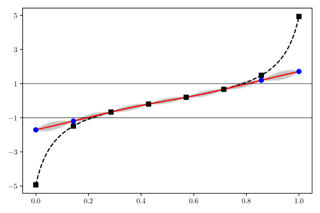
Figure 4: An example of reGP predictive distribution with $R=\left(-\infty,-1\right]\cup\left[1,+\infty\right)$ on a function $f$ represented in dashed black lines. The solid black lines represent the relaxation thresholds. The problem (15) was solved only in $\underline{z}$ as the parameters of the (constant) mean and ($\nu=5/2$ Matérn) covariance functions were held fixed for illustration purposes.

Remark 8 (Numerical details)

Minimizing (15) with respect to $\underline{z}$ falls under the scope of quadratic programming (see, e.g., Nocedal and Wright, 2006) and could be solved efficiently using dedicated algorithms. This suggests that specific algorithms could be developed for the problem. In this work, we simply use a standard L-BFGS-B solver (Byrd et al., 1995) using the gradient of (15).

3.3 Convergence Analysis of reGP

In this section, we provide several theoretical results concerning the convergence of the method proposed. This section can be skipped on first reading.

3.3.1 Known Convergence Results about Interpolation in RKHS

Recall that the fractional-order Sobolev space $W_{2}^{\beta}(\mathds{R}^{d})$, with regularity $\beta\geq 0$, is the space of functions on $\mathds{R}^{d}$ defined by

$$W_{2}^{\beta}(\mathds{R}^{d})=\Bigl{\{}h\in L^{2}(\mathds{R}^{d}),\,\lVert h\rVert_{W_{2}^{\beta}(\mathds{R}^{d})}=\bigl{\lVert}\widehat{h}\,\left(1+\lVert\cdot\rVert^{2}\right)^{\beta/2}\bigr{\rVert}_{L^{2}(\mathds{R}^{d})}<+\infty\Bigr{\}},$$

where $\widehat{h}\in L^{2}(\mathds{R}^{d})$ is the Fourier transform of $h\in L^{2}(\mathds{R}^{d})$.

For a given $\mathds{X}\subset\mathds{R}^{d}$, define the Sobolev spaces $W_{2}^{\beta}(\mathds{X})=\bigl{\{}h_{\lvert\mathds{X}},\,h\in W_{2}^{\beta}(\mathds{R}^{d})\bigr{\}}$ endowed with the norm

$$\lVert h\rVert_{W_{2}^{\beta}(\mathds{X})}=\inf_{g\in W_{2}^{\beta}(\mathds{R}^{d}),\,g_{\lvert\mathds{X}}=h}\lVert g\rVert_{W_{2}^{\beta}(\mathds{R}^{d})}.$$ (17)

The following assumption about $\mathds{X}$ will sometimes be used in this section.

Assumption 1

The domain is non-empty, compact, connected, has locally Lipschitz boundary (see, e.g., Adams and Fournier, 2003, Section 4.9), and is equal to the closure of its interior.

Assumption 1 ensures that the previous definition coincides with other commons definitions, and makes it possible to use well-known results from the field of scattered data approximation, by preventing the existence of cusps. Many common domains—such as hyperrectangles or balls, for instance—verify Assumption 1.

A strictly positive-definite reproducing kernel $k:\mathds{X}\times\mathds{X}\to\mathds{R}$ is said to have regularity $\alpha>0$ if the associated RKHS $\mathcal{H}(\mathds{X})$ coincides with $W_{2}^{\alpha+d/2}(\mathds{X})$ as a function space, with equivalent norms. As such, the Matérn stationary kernels (4) have correlation functions $r$ whose Fourier transform verifies (see, e.g., Wendland, 2004, Theorem 6.13)

$$C_{1}\left(1+\lVert\cdot\rVert^{2}\right)^{-\nu-d/2}\leq\widehat{r}\leq C_{2}\left(1+\lVert\cdot\rVert^{2}\right)^{-\nu-d/2}$$

for some $C_{2}\geq C_{1}>0$, and have therefore Sobolev regularity $\alpha=\nu$ on $\mathds{R}^{d}$ (see, e.g., Wendland, 2004, Corollary 10.13) and consequently also on $\mathds{X}$, using (17) and Lemma 24. Other examples are given by Wendland (2004), for instance.

We now recall a classical convergence result about interpolation in RKHS with evaluation points in a bounded domain. Consider a kernel $k:\mathds{X}\times\mathds{X}\to\mathds{R}$, and let $\left(x_{n}\right)_{n\geq 1}\in\mathds{X}^{\mathds{N}}$ be a sequence of distinct points. The following property (a minor reformulation of Theorem 4.1 of Arcangéli et al. (2007)) gives error bounds that depend on the Sobolev regularity of $k$ and the so-called fill distance of $\underline{x}_{n}\in\mathds{X}^{n}$, defined by

$$h_{n}=\sup_{x\in\mathds{X}}\min_{1\leq i\leq n}\lVert x-x_{i}\rVert.$$ (18)

Proposition 9

Let $k$ be a reproducing kernel with regularity $\alpha>0$. If $\mathds{X}$ verifies Assumption 1, then

$$\sup_{x\in\mathds{X}}\sigma_{n}(x)\lesssim h_{n}^{\alpha},\quad n\geq 1\,,$$ (19)

where $\lesssim$ denotes inequality up to a constant, that does not depend on $\left(x_{n}\right)_{n\geq 1}$.

Using (9) and Proposition 9, this yields the following uniform bound.

Corollary 10

Let $k$ be a reproducing kernel with regularity $\alpha>0$, $\mathcal{H}(\mathds{X})$ the RKHS generated by $k$, and let $f\in\mathcal{H}(\mathds{X})$. As above, let $s_{\underline{z}_{n}}$ be the solution of (8) for $\underline{z}_{n}=\left(f(x_{1}),\cdots,f(x_{n})\right)^{\mathsf{T}}$, $n\geq 1$. If $\mathds{X}$ verifies Assumption 1, then

$$\lVert f-s_{\underline{z}_{n}}\rVert_{L^{\infty}(\mathds{X})}\lesssim h_{n}^{\alpha}\lVert f\rVert_{\mathcal{H}(\mathds{X})}\,.$$ (20)

3.3.2 Convergence Results for reGP

Let $k\colon\mathds{X}\times\mathds{X}\to\mathds{R}$ be a continuous strictly positive-definite reproducing kernel. In this section, we consider the zero-mean reGP predictive distribution obtained from $\xi\sim\mathop{\mathrm{GP}}(0,\,k)$, with relaxed interpolation constraints on a union $R=\bigcup_{j=1}^{q}R_{j}$ of disjoints closed intervals $R_{j}$ with non-zero length. Let $\mathcal{H}(\mathds{X})$ be the RKHS attached to $k$, $f\in\mathcal{H}(\mathds{X})$, and consider a sequence $\left(x_{n}\right)_{n\geq 1}\in\mathds{X}^{\mathds{N}}$ of distinct points. Furthermore, define (the) regions $\mathds{X}_{j}=\{x\in\mathds{X},\ f(x)\in R_{j}\}$ for $1\leq j\leq q$ and $\mathds{X}_{0}=\mathds{X}\setminus\bigcup_{j\geq 1}\mathds{X}_{j}$. We give results about the limit of the sequence of reGP predictive distributions that suggest an improved fit in $\mathds{X}_{0}$.

Let $s_{R,\,n}=s_{\underline{z}_{n}^{\star}}$ be the relaxed predictor from Proposition 3 based on $\left(x_{1},\cdots,x_{n}\right)$ and $\left(f(x_{1}),\cdots,f(x_{n})\right)^{\mathsf{T}}$, $n\geq 1$. The following proposition establishes the limit behavior of $(s_{R,\,n})_{n\geq 1}$.

Proposition 11

Let $\mathds{U}\subset\mathds{X}$ and let $\mathcal{H}_{R,\,\mathds{U}}$ denote the set of functions $h\in\mathcal{H}(\mathds{X})$ such that, for all $x\in\mathds{U}$,

$$\left\{\begin{array}[]{llll}h(x)\in R_{j}&\mathrm{if}\ f(x)\in R_{j}\ \mathrm{for\ some}\ j,\\ h(x)=f(x)&\mathrm{otherwise}.\\ \end{array}\right.$$ (21)

Then the problem

$$\min_{h\in\mathcal{H}_{R,\,\mathds{U}}}\lVert h\rVert_{\mathcal{H}(\mathds{X})}$$ (22)

has a unique solution denoted by $s_{R,\mathds{U}}$. Moreover,

$$s_{R,n}\xrightarrow{\mathcal{H}(\mathds{X})}s_{R,\mathds{U}},$$ (23)

with $\mathds{U}$ the closure of $\{x_{n}\}$.

In particular, when $\{x_{n}\}$ is dense in $\mathds{X}$, then $\mathds{U}=\mathds{X}$ and $(s_{R,\,n})_{n\geq 1}$ converges to $s_{R,\,\mathds{X}}$, which is the minimal-norm element of the set $\mathcal{H}_{R,\,\mathds{X}}$.

The next proposition tells us that the interpolation error on $\mathds{X}_{0}$ can be bounded by a term that depends on the norm of $s_{R,\,\mathds{X}}$.

Proposition 12

For any $x\in\mathds{X}_{0}$ and $n\geq 1$,

$$\lvert f(x)-s_{R,\,n}(x)\rvert\leq 2\sigma_{n,\,0}(x)\lVert s_{R,\,\mathds{X}}\rVert_{\mathcal{H}(\mathds{X})},$$ (24)

where $\sigma_{n,\,0}$ is the power function obtained using only points in $\mathds{X}_{0}$ for predictions.

This yields the following error bounds when the design is dense.

Proposition 13

Suppose that $\{x_{n}\}$ is dense and that $k$ has regularity $\alpha>0$. Let $B\subset\mathds{X}_{0}$ verify Assumption 1. Then, for all $n\geq 1$,

$$\lVert f-s_{R,\,n}\rVert_{L^{\infty}(B)}\lesssim h_{n}^{\alpha}\lVert s_{R,\,\mathds{X}}\rVert_{\mathcal{H}(\mathds{X})}.$$ (25)

Let $d(y,\,A)$ be the distance of $y\in\mathds{R}$ to $A\subset\mathds{R}$. For $j\geq 1$, $x\in\mathds{X}_{j}$, and for all $n\geq 1$:

$$d(s_{R,\,n}(x),\,R_{j})\lesssim h_{n}^{\alpha}\lVert s_{R,\,\mathds{X}}\rVert_{\mathcal{H}(\mathds{X})}\quad\mathrm{if}\ \alpha<1,$$ (26)

$$d(s_{R,\,n}(x),\,R_{j})\lesssim\sqrt{\left(\lvert\ln(h_{n})\rvert+1\right)}\,h_{n}\,\lVert s_{R,\,\mathds{X}}\rVert_{\mathcal{H}(\mathds{X})}\quad\mathrm{if}\ \alpha=1,$$ (27)

and

$$d(s_{R,\,n}(x),\,R_{j})\lesssim h_{n}\lVert s_{R,\,\mathds{X}}\rVert_{\mathcal{H}(\mathds{X})}\quad\mathrm{if}\ \alpha>1\,,$$ (28)

where $\lesssim$ denotes inequality up to a constant, that does not depend on $f$, $n$ or $(x_{n})$.

Finally, we investigate the following question: how large can be the norm of $f$ compared to the approximation $\lVert s_{R,\,\mathds{X}}\rVert_{\mathcal{H}(\mathds{X})}$?

Proposition 14

Suppose that $k$ has regularity $\alpha>0$ and that there exists some $j\geq 1$ such that $\mathds{X}_{j}$ has a non-empty interior. We have

$$\sup_{h\in\mathcal{H}_{R,\,\mathds{X}}}\lVert h\rVert_{\mathcal{H}(\mathds{X})}=+\infty,$$ (29)

with $\mathcal{H}_{R,\,\mathds{X}}$ given by (21) for $f\in\mathcal{H}(\mathds{X})$.

This result shows that the norm reduction obtained by approximating $f$ with relaxed interpolation constraints can therefore be arbitrarily high in the finite-smoothness case. A stronger version of Proposition 14 for the special case where $R=[t,+\infty)$ can be derived, and shows that

$$\sup_{h\in\mathcal{H}_{R,\,\mathds{X}}}\lVert h\rVert_{L^{\infty}(\mathds{X})}=+\infty\,.$$

Overall, no matter the element of $\mathcal{H}_{R,\,\mathds{X}}$ at hand, reGP converges to a function $s_{R,\,\mathds{X}}$ which: coincides with $f$ on $\mathds{X}_{0}$, verifies $f(x)\in R_{j}\Leftrightarrow s_{R,\,\mathds{X}}(x)\in R_{j}$ for all $x\in\mathds{X}$, and is “nicer” than $f$ in the sense of $\lVert\cdot\rVert_{\mathcal{H}(\mathds{X})}$. Furthermore, reGP yields error bounds carrying the norm of $s_{R,\,\mathds{X}}$, which can be arbitrarily smaller than the norm of $f$ in the case of a finite-smoothness covariance function.

Remark 15

Note that $\sigma_{n}\leq\sigma_{n,\,0}$ due to the projection residuals interpretation. Empirical and theoretical results about the screening effect (see, e.g., Stein, 2011; Bao et al., 2020), suggests that $\sigma_{n}\simeq\sigma_{n,\,0}$, if $k$ has smoothness $\alpha>0$. In this case, observe that—no matter the element of $\mathcal{H}_{R,\,\mathds{X}}$ at hand—the bound (24) is larger by only a small factor compared to (9) with $f=s_{R,\,\mathds{X}}$. (However, to the best of our knowledge, no result exists concerning the screening effect for arbitrary designs.)

Remark 16

The equality (29) does not hold in general for infinitely smooth covariance functions. For instance, Steinwart et al. (2006, Corollary 3.9) show that $\mathcal{H}_{R,\,\mathds{X}}=\{f\}$ if the interior of $\mathds{X}_{0}$ is not empty and $k$ is the squared-exponential covariance function (i.e. (4), with $\nu\to\infty$).

4 Choice of the Relaxation Set

4.1 Towards Goal-Oriented Cross-Validation

The framework of reGP makes it possible to predict a function $f$ from point evaluations of $f$. Suppose we are specifically interested in obtaining good predictive distributions in a range $Q\subset\mathds{R}$ of function values, and accept degraded predictions outside this range. To achieve this goal, the idea of reGP is to relax interpolation constraints. Naturally, it makes sense to relax interpolation constraints outside the range $Q$ but it could happen that relaxing interpolation constraints does not improve predictive distributions on $Q$. Therefore, the question arises as to how to automatically select a range $R$ in $\mathds{R}\setminus Q$, on which interpolation constraints should be relaxed.

In the following, we put $R^{(0)}=\mathds{R}\setminus Q$, and we view the relaxation set $R$ as a parameter of the reGP model, which has to be chosen in $R^{(0)}$ along with the parameters $\theta$ of the underlying GP $\xi$. A first idea for the selection of $R$ is to rely on the standard leave-one-out cross-validation approach to select the parameters of a GP (Dubrule, 1983; Rasmussen and Williams, 2006; Zhang and Wang, 2010). Using the formalism of scoring rules (see, e.g., Gneiting and Raftery, 2007; Petit et al., 2021), selecting parameters by a leave-one-out approach amounts to minimizing a selection criterion written as

$$J_{n}(R)=\frac{1}{n}\sum_{i=1}^{n}S\left(P_{R,\,n,\,-i},\,f(x_{i})\right),$$ (30)

where $P_{R,\,n,\,-i}$ is reGP predictive distribution with data $\underline{z}_{n,-i}=(z_{1},\,\ldots,z_{i-1},\,z_{i+1},\,\ldots,z_{n})$ and relaxation set $R$. The function $S$ in (30) is a scoring rule, that is, a function $S:\mathcal{P}\times\mathds{R}\to\mathds{R}\cup\left\{-\infty,+\infty\right\}$, acting on a class $\mathcal{P}$ of probability distributions on $\mathds{R}$, such that $S(P,\,z)$ assigns a loss for choosing a predictive distribution $P\in\mathcal{P}$, while observing $z\in\mathds{R}$. Scoring rules make it possible to quantify the quality of probabilistic predictions.

Since the user is not specifically interested in good predictive distributions in $R^{(0)}$, validating the model on $R^{(0)}$ should not be a primary focus. However, simply restricting the sum (30) by removing indices $i$ such that $f(x_{i})\in R^{(0)}$ would make it impossible to assess if the model is good at predicting that $f(x)\in R^{(0)}$ for a given $x\in\mathds{X}$. For instance, in the case of minimization, with $Q=(-\infty,\,t^{(0)})$ and $R^{(0)}=[\,t^{(0)},\infty)$, it is important to identify the regions corresponding to $f$ being above $t^{(0)}$, even if we are not interested in accurate predictions above $t^{(0)}$, because we expect that an optimization algorithm should avoid the exploration of these regions.

In the next section, we propose instead to keep the whole leave-one-out sum (30), but to choose a scoring rule $S$ that serves our goal-oriented approach.

4.2 Truncated Continuous Ranked Probability Score

An appealing class of scoring rules for goal-oriented predictive distributions is the class of weighted scoring rules for binary predictors (Gneiting and Raftery, 2007; Matheson and Winkler, 1976), which may be written as

$$S\left(P,\,z\right)=\int_{-\infty}^{+\infty}s(F_{P}(u),\mathds{1}_{z\leq u})\,\mu(\mathrm{d}u)\,,$$ (31)

where $s\colon\left[0,\,1\right]\times\{0,\,1\}\to\mathds{R}\cup\{-\infty,+\infty\}$ is a scoring rule for binary predictors, and $\mu$ is a Borel measure on $\mathds{R}$. A well-known instance of (31) is the continuous ranked probability score (Gneiting et al., 2005) written as

$$S^{\mathrm{CRPS}}(P,\,z)=\int_{-\infty}^{+\infty}\left(F_{P}(u)-\mathds{1}_{z\leq u}\right)^{2}\mathrm{d}u\,,$$

which is obtained by choosing the Brier score for $s$ and the Lebesgue measure for $\mu$.

For the case where we are specifically interested in obtaining good predictive distributions in a range of interest $Q\subset\mathds{R}$, we propose to use the following scoring rule, which we call truncated continuous ranked probability score (tCRPS):

$$S_{Q}^{\mathrm{tCRPS}}(P,\,z)\;=\;\int_{Q}\left(F_{P}(u)-\mathds{1}_{z\leq u}\right)^{2}\mathrm{d}u.$$ (32)

This scoring rule, proposed by Lerch and Thorarinsdottir (2013) in a different context, reduces to $S^{\mathrm{CRPS}}$ when $Q=\mathds{R}$. It can be seen as a special case of the weighted CRPS (Matheson and Winkler, 1976; Gneiting and Raftery, 2007; Gneiting and Ranjan, 2011), in which the indicator function $\mathds{1}_{Q}$ plays the role of the weight function—in other words, the measure $\mu$ in (31) has density $\mathds{1}_{Q}$ with respect to Lebesgue’s measure.

Consider for instance the case $Q=\left(-\infty,\,t^{(0)}\right)$:

$$S_{Q}^{\mathrm{tCRPS}}(P,\,z)\;=\;\int_{-\infty}^{t^{(0)}}\left(F_{P}(u)-\mathds{1}_{z\leq u}\right)^{2}\mathrm{d}u.$$ (33)

The upper endpoint $t^{(0)}$ of the range will be referred to as the validation threshold. Note that, in this case, $S_{Q}^{\mathrm{tCRPS}}(P,\,z)$ does not depend on the specific value of $z$ when $z$ is above the validation threshold. This scoring rule is thus well suited to the problem of measuring the performance of a predictive distribution in such a way as to fully assess the goodness-of-fit of the distribution when the true value is below a threshold, and only ask that the support of the predictive distribution is concentrated above the threshold when the true value is above the threshold.

We provide in Appendix A some properties of the scoring rule (32) and closed-form expressions for the case where $Q$ is an interval (or a finite union of intervals) and $P$ is Gaussian. To the best of our knowledge, these expressions are new.

4.3 Choosing the Relaxation Set using the tCRPS Scoring Rule

Given a range of interest $Q$, the tCRPS scoring rule makes it possible to derive a goal-oriented leave-one-out selection criterion, that we shall call the LOO-tCRPS criterion:

$$J_{n}\left(R\right)=\frac{1}{n}\sum_{i=1}^{n}S_{Q}^{\mathrm{tCRPS}}\left(P_{R,\,n,\,-i},\,f(x_{i})\right)\,.$$ (34)

Using (34), we suggest the following procedure to select a reGP model. First, choose a sequence of nested candidate relaxation sets $R^{(0)}\supset R^{(1)}\supset\cdots\supset R^{(G)}=\emptyset$. The next step is the computation of $J_{n}(R^{(g)})$, $g=0,\,\ldots,\,G$, which involves the predictive distributions $P_{R^{(g)},\,n,\,-i}$.

In principle, (15) should be solved again each time a data point $(x_{i},\,z_{i})$ is removed, to obtain a pair $(\widehat{\theta}_{n,-i}^{(g)},\,\underline{z}_{n,-i}^{(g)})$ and then the corresponding reGP distribution $P_{R^{(g)},\,n,\,-i}$. To alleviate computational cost, a simple idea is to rely on the fast leave-one-out formulas (Dubrule, 1983) for Gaussian processes: for each set $R^{(g)}$, solve (15) to obtain $\widehat{\theta}_{n}^{(g)}$ and $\underline{z}_{n}^{(g)}=(z_{1}^{(g)},\,\ldots,\,z_{n}^{(g)})^{\mathsf{T}}$, and then compute the conditional distributions $\xi(x_{i})\mid\{\xi(x_{j})=z_{j}^{(g)},j\neq i\}$, where $\xi\sim\mathop{\mathrm{GP}}(\mu,\,k)$, and where $\mu$ and $k$ have parameter $\widehat{\theta}_{n}^{(g)}$, using the fast leave-one-out formulas. By doing so, we neglect the difference between $\widehat{\theta}_{n,-i}^{(g)}$ and $\widehat{\theta}_{n}^{(g)}$ and the difference between $\underline{z}_{n,-i}^{(g)}$ and the vector $(z_{1}^{(g)},\,\ldots,\,z_{i-1}^{(g)},\,z_{i+1}^{(g)},\,\ldots,\,z_{n}^{(g)})^{\mathsf{T}}$.

The procedure ends by choosing the relaxation set $R^{(g)}$ that achieves the best LOO-tCRPS value.

Figure 5 illustrates the selection of the relaxation set used in Figure 3.

Figure 5: Illustration of the choice of a relaxation set. The range of interest $Q$ is determined by the threshold $t^{(0)}$. The relaxation set $R$ corresponding to the region above $t$ has been obtained by the procedure described in Section 4.3.

4.4 An Example for the Estimation of an Excursion Set

We illustrate the method on the problem of estimating an excursion set $\{x\in\mathds{X},\,f(x)\leq 0\}$. We consider the G10 optimization problem used by Regis (2014), and focus on the constraint $c_{6}\leq 0$. Finding solutions satisfying the $c_{6}\leq 0$ constraint using a GP model is difficult, probably because the values of $c_{6}$ are very bi-modal, as illustrated in Figure 6. However, Feliot et al. (2017) found that the difficulty could be overcome by performing an ad-hoc monotonic transformation $z\mapsto z^{\alpha}$, with $\alpha=7$, on the constraint.

Figure 6: Left: Histogram of the values of the function $c_{6}$ from the G10 problem. Right: Same illustration but for the function $c_{6}^{\alpha}$, with $\alpha=7$. The histograms are obtained from the values of the functions on a space-filling design of size $n=100$. On the left, the values are very separated and concentrated on two modes, yielding a function close to a piecewise constant function. After transformation, the phenomenon is mitigated.

The estimation of an excursion set $\left\{f\leq 0\right\}$ involves capturing precisely the behavior of $f$ around zero. Thus, we define a range of interest $Q=(-t^{(0)},\,t^{(0)})$ centered on zero, with $t^{(0)}$ sufficiently small (note that there may be no data in $Q$). Then, we consider relaxation range candidates $R^{(g)}=(-\infty,-t^{(g)}\,]\cup[\,t^{(g)},+\infty)$ with a sequence of thresholds $t^{(0)}<\cdots<t^{(G)}=+\infty$, and we select $t^{(g)}$ by minimizing the LOO-tCRPS as described in the previous section.

In the case of the $c_{6}$ constraint and a small value for $t^{(0)}$ such that there is no data in $Q$, the results are presented in Figure 7. The LOO-tCRPS chooses $t^{(g)}=t^{(0)}$, so the reGP predictive distributions use only the information of being above or below zero. Moreover, observe that the corresponding transformation after relaxation bears resemblance to the transformation $z\mapsto z^{\alpha}$ proposed by Feliot et al. (2017). If we apply the reGP framework on the transformed function $c_{6}^{\alpha}$ (details omitted for brevity), we find that the LOO-tCRPS chooses a large $t^{(g)}$ such that the interpolation constraints are relaxed for a few observations only.

Figure 7: A reGP fit of $c_{6}$, where the relaxation thresholds have been selected by LOO-tCRPS. The observations $\underline{z}_{n}$ are shown on the $x$-axis, whereas the “relaxed” observations $\underline{z}_{n}^{\star}$ are represented on the $y$-axis. Moreover, the green lines represent the value zero, and the brown lines represent $\pm\ t^{(g)}$, with $t^{(g)}$ chosen to be $t^{(0)}$ by the LOO-tCRPS. Finally, the blue line shows a best fit by $z\mapsto z^{7}$.

5 Application to Bayesian Optimization

5.1 Efficient Global Optimization with Relaxation

The first motivation for introducing reGP models is Bayesian optimization, where obtaining good predictive distributions over ranges corresponding to optimal values is a key issue. In this article, we focus more specifically on the minimization problem

$$\min_{x\in\mathds{X}}f(x)\,,$$ (35)

where $f$ is a real-valued function defined on a compact set $\mathds{X}\subset\mathds{R}^{d}$, but the methodology can be generalized to constrained and/or multi-objective formulations.

Given $f$, our objective is to construct a sequence of evaluation points $X_{1},X_{2}\,\ldots\in\mathds{X}$ by choosing each point $X_{n+1}$ as the maximizer of the expected improvement criterion (6) computed with respect to the reGP predictive distribution, with a relaxation set $R_{n}=\left[t_{n},+\infty\right)$. More precisely, the sequence $(X_{n})$ is constructed sequentially using the rule

$$X_{n+1}\;=\;\operatorname*{arg\,max}_{x\in\mathds{X}}\;\mathsf{E}_{n}\left(\left(m_{n}-\xi(x)\right)_{+}\right)\,,$$ (36)

where $m_{n}=f(X_{1})\wedge\cdots\wedge f(X_{n})$, and $\mathsf{E}_{n}$ is the expectation under the reGP predictive distribution with relaxation set $R_{n}$ and data $\underline{z}_{n}=(f(X_{1}),\,\ldots,\,f(X_{n}))^{\mathsf{T}}$.

As in Section 4.3, the relaxation threshold $t_{n}$ at iteration $n$ is chosen using the LOO-tCRPS criterion (34) among candidate values

$$t_{n}^{(0)}<t_{n}^{(1)}<\cdots<t_{n}^{(G)}\,,$$ (37)

where $t_{n}^{(0)}$ is the validation threshold, which delimits the range of interest $Q_{n}=\bigl{(}-\infty,t_{n}^{(0)}\bigr{)}$ used at iteration $n$. In the following, the optimization method just described will be called efficient global optimization with relaxation (EGO-R), in reference to the EGO name proposed by Jones et al. (1998).

Implementation specifics are detailed in Section 5.3. In the next section, we show that using the EI criterion with a reGP model yields a convergent algorithm.

5.2 Convergence of EGO-R with Fixed Parameters and Varying Threshold

In this section, we extend the result of Vazquez and Bect (2010b) and show the convergence of the EGO-R algorithm, in the case where the predictive distributions derive from a zero-mean Gaussian process with fixed covariance function.

We suppose that $\mathds{X}$ is a compact domain and that $k:\mathds{X}\times\mathds{X}\to\mathds{R}$ is continuous, strictly positive-definite, and has the NEB (no-empty ball) property (Vazquez and Bect, 2010b), which says that the posterior variance cannot go to zero at a given point if there is no evaluation points in a ball centered on this point. In other words, the NEB property requires that the posterior variance $\sigma_{n}^{2}(x)$ at $x\in\mathds{X}$ remains bounded away from zero for any $x$ not in the closure of the sequence of points $(X_{n})$ evaluated by the optimization algorithm. A stationary covariance function with smoothness $\alpha>0$ verifies the NEB property (Vazquez and Bect, 2010b), whereas the squared-exponential covariance function does not (Vazquez and Bect, 2010a).

Proposition 17

Let $k:\mathds{X}\times\mathds{X}\to\mathds{R}$ be a continuous strictly positive-definite covariance function that verifies the NEB property, $\mathcal{H}(\mathds{X})$ the corresponding RKHS and $f\in\mathcal{H}(\mathds{X})$. Let $n_{0}>0$. Let $\left(X_{n}\right)_{n\geq 1}$ be a sequence in $\mathds{X}$ such that, for each $n\geq n_{0}$, $X_{n+1}$ is obtained by (36) with $t_{n}>m_{n}$. Then the sequence $\left(X_{n}\right)_{n\geq 1}$ is dense in $\mathds{X}$.

Proposition 17 implies the convergence of EGO-R with a fixed threshold $t>\min_{i\leq n_{0}}f(X_{i})$. In this case, the theoretical insights from Section 3.3 suggest a faster convergence might be achieved due to the improved error estimates (24) and (25) in a neighborhood of the global minimum.

The convergence of EGO-R also holds in the case of a varying relaxation set $R_{n}=\left[t_{n},+\infty\right)$, with $t_{n}>m_{n}$, and in particular when $t_{n}$ is selected at each step using the LOO-tCRPS criterion (34) with a validation threshold $t_{n}^{(0)}>m_{n}$. In this case, the norm term in (24) gets smaller if $\left(t_{n}\right)_{n\geq 1}$ is decreasing.

5.3 Optimization Benchmark

In this section, we run numerical experiments to demonstrate the interest of using EGO-R instead of EGO for minimization problems.

5.3.1 Methodology

In practice, we must choose the sequence of thresholds (37). The validation threshold $t_{n}^{(0)}$ should be set above $m_{n}$ to ensure there is enough data to carry out the validation. We propose two different heuristics: a) a constant heuristic, where $t_{n}^{(0)}$ is kept constant through the iterations and set to an empirical quantile of an initial data set constructed before EGO-R is run, and b) a concentration heuristic, where $t_{n}^{(0)}$ corresponds to an empirical quantile of $\underline{z}_{n}$.

In the case of the constant heuristic, we set $t_{n}^{(0)}$ to the $\alpha$-quantile of the function values on an initial design, which is typically built to fill $\mathds{X}$ as evenly as possible with, e.g., maximin Latin hypercube sampling (McKay et al., 2000). The numerical experiments were conducted with $\alpha=0.25$ in this article.

In the case of the concentration heuristic, we consider an $\alpha$-quantile of the values of $f$ at the points visited by the algorithm (again with $\alpha=0.25$). As the optimization algorithm makes progress, the evaluations will likely concentrate around the global minimum. Thus, $t_{n}^{(0)}$ will get closer to the minimum value, and the range $Q_{n}=(-\infty,\,t_{n}^{(0)})$ of validation values will get smaller. Besides, since we expect better predictive distributions in this range, a better convergence may be obtained.

Both heuristics can be justified by the idealized setting of the convergence result from the previous section. Proposing alternative adaptive strategies to the concentration heuristic, or more generally conducting a theoretical study on the performance of such adaptive strategies, is out of the scope of this article.

For a given $t_{n}^{(0)}$, the candidate relaxation thresholds $t_{n}^{(g)}$, $g=1,\,\ldots,\,G$, are chosen so that $t_{n}^{(g)}-m_{n}$ ranges logarithmically from $t_{n}^{(0)}-m_{n}$ to $\max f(X_{i})-m_{n}$ (with $G=10$, in the experiments below).

To assess the performances of EGO-R with the two heuristics for choosing $t_{n}^{(0)}$, we compare them to the standard EGO algorithm. For all three algorithms, we use a first initial design of size $n_{0}=3d$, and we consider GPs with constant mean and a Matérn covariance function with regularity $\nu=5/2$. The maximization of the sampling criteria (6) and (36) is carried out using a sequential Monte Carlo approach (Benassi et al., 2012; Feliot et al., 2017).

For reference, we also run the Dual simulated Annealing algorithm (inspired by Xiang et al. (1997)) from SciPy (Virtanen et al., 2020), with the default settings and with a random initialization.

The optimization algorithms are tested against a benchmark of test functions from Surjanovic and Bingham (2013) summarized in Table 1, with $n_{\mathrm{rep}}=30$ (random) repetitions, and a budget of $n_{\mathrm{tot}}=300$ evaluations for each repetition. This benchmark is partly inspired by Jones et al. (1998) and Merrill et al. (2021). In particular, we also use a log-version of the Goldstein-Price function as Jones et al. (1998).

Table 1: Optimization benchmark. The acronym G-P stands for Goldstein-Price.

Problem	$d$
Branin	$2$
Six-hump Camel	$2$
Three-hump Camel	$2$
Hartman	$3$, $6$
Ackley	$4$, $6$, $10$
Rosenbrock	$4$, $6$, $10$
Shekel	$5$, $7$, $10$
Goldstein-Price	$2$
Log-Goldstein-Price	$2$
Cross-in-Tray	$2$
Beale	$2$
Dixon-Price	$4$, $6$, $10$
Perm	$4$, $6$, $10$
Michalewicz	$4$, $6$, $10$
Zakharov	$4$, $6$, $10$

To evaluate the algorithms we use, for each test function, several targets defined as spatial quantiles of the function and estimated with a subset simulation algorithm (see, e.g., Au and Beck, 2001). Then, the performances of the algorithms are evaluated using the fractions of runs that manage to reach the targets and the average numbers of evaluations to reach the targets (with unsuccessful runs counted as $n_{\mathrm{tot}}$).

5.3.2 Findings

The full set of results is provided in Appendix C. In Figure 8, we present a representative subset of these results.

First, observe in Figure 8 that the EGO-R methods can be considerably helpful and can outperform EGO largely on functions that are difficult to model with stationary GPs, such as Goldstein-Price, Perm ($10$), and Beale.

Observe also that the EGO-R methods have about the same performance as EGO on functions that are easy to model with stationary GPs. This is the case of the Log-Goldstein-Price and the Branin functions, for which the LOO-tCRPS criterion for choosing the relaxation set detects that the larger values help predict near the minimum, and that no relaxation is needed as a result.

Furthermore, it is instructive to compare the performances of the EGO-R algorithms on the Goldstein-Price function on the one hand, with the performance of the EGO algorithm on Log-Goldstein-Price function on the other hand. Using reGP modeling enables to perform as well as with the logarithmic transform, but in an automatic way. This is also illustrated by Figure 9, which shows that the (non-parametric) transform learned by reGP resembles a logarithmic transform.

Finally, observe that the constant heuristic performs as well as EGO on Ackley $(10)$, whereas the concentration heuristic lags behind. A closer look at the results for this function shows that the concentration heuristic get sometimes stuck in a local minimum. We explain this by the fact that the reGP model with the concentration heuristic can become very predictive in a small region around the local minimum, and underestimate the function variations elsewhere (the variance of the predictive distributions above $t_{n}^{(0)}$ are too small, and the optimization algorithm does not sufficiently explore unknown regions). To this regard, the constant heuristic is probably more conservative. Overall, taking the results from Appendix C into account, the concentration heuristic appears to be more (resp. less) efficient than the constant heuristic when there are few (resp. many) local minima.

Figure 8: For each case, the top plot is the average number of iterations to reach the spatial quantile, and the bottom plot is the proportion of successful runs. Both are represented versus the level of the spatial quantile. The gray dotted line stands for the Dual simulated Annealing algorithm, the red line for the standard EGO algorithm, and the blue and green lines for EGO-R, with the “Constant” and “Concentration” heuristics. The results are shown until the success rates of the three previous methods fall below the $66\%$ threshold materialized by the black dashed line.

Figure 9: A reGP fit to the Goldstein-Price function with $n=30$ points, with $R=\left[10^{3},\,+\infty\right)$. The observations $\underline{z}_{n}$ are shown on the $x$-axis, whereas the relaxed observations $\underline{z}_{n}^{\star}$ are represented on the $y$-axis.

6 Conclusion

This article presents a new technique called reGP to build predictive distributions for a function observed on a sequence of points. This technique can be applied when a user wants good predictive distributions in a range of function values, for example below a given threshold, and accepts degraded predictions outside this range. The technique relies on Gaussian process interpolation, and operates by relaxing the interpolation constraints outside the range of interest. This goal-oriented technique is kept simple and cheap: there are no additional parameters to set compared to the standard Gaussian process framework. The user only needs to specify a range of function values where good predictions should be obtained. The relaxation range can be selected automatically, using a scoring rule adapted to reGP models.

Such goal-oriented models can then be used in Bayesian sequential search algorithms. Here we are interested in the problem of mono-objective optimization and we propose to study the EI / EGO algorithm with such models. In a first step, we guarantee the convergence of the reGP-based algorithm on the RKHS attached to the underlying GP covariance. Then, we provide a benchmark that shows very clear benefits of using reGP models for the optimization of various functions.

A key element of the reGP approach is the definition of a range of interest $Q$, for instance a range of the form $\left(-\infty,t^{(0)}\right)$ in a minimization problem. In some use cases the range will be provided by the user, but in others it is desirable to set it automatically. Two simple heuristics have been proposed in Section 5.3 to achieve this goal in our optimization benchmark, and it has been observed that the choice of heuristic has an impact on the exploratory behaviour of the resulting Bayesian optimization algorithm. Finding better heuristics, studying their properties, and assessing their impact in Bayesian optimization applications, is an important direction for future research.

More generally, the goal-oriented approach proposed in this article is not limited to single-objective (Bayesian) optimization. The example of Section 4.4 shows that it is also readily applicable, for instance, to level set estimation problems, for which a number of GP-based sequential design—aka active learning—strategies have been proposed in the literature (see, e.g., Chevalier et al., 2014; Bogunovic et al., 2016, and references therein). Other extensions are possible but will require more work. Noisy observations are one such example: considering that the interpolation constraints are already relaxed by the presence of noise, how should we transpose the goal-oriented modeling approach to this setting? Constrained and/or multi-objective optimization is another interesting but challenging direction for future research: in this case the function of interest in multivariate—one objective and several constraints, or several objectives—which requires significant adaptations to proposed methodology.

A Properties of the Truncated CRPS

We shall now write (32) more explicitly for the case where the range of interest is an interval $Q=(a,b)$, $-\infty\leq a<b\leq+\infty$, and provide closed-form expressions for the case where, in addition, the predictive distribution $P$ is Gaussian.

Remark 18

The value of the tCRPS for an interval $Q=(a,b)$ remains unchanged if the interval is closed at one or both of its endpoints.

Remark 19

The value of the tCRPS for a finite (or countable) union of disjoint intervals follows readily from its values on intervals, since $Q\mapsto S_{Q}^{\mathrm{tCRPS}}(P,\,z)$ is $\sigma$-additive.

We shall start by defining a quantity that shares similarities with (6).

Definition 20

$\mathrm{EI}_{q}^{\uparrow}(P,\,z)\;=\;\mathsf{E}\left(\left(N_{1}\vee\cdots\vee N_{q}-z\right)_{+}\right)$ with $N_{j}\stackrel{{\scriptstyle\mathrm{iid}}}{{\sim}}P$.

The following expressions hold for a general predictive distribution $P$.

Proposition 21

Suppose that $P$ has a first order moment.

• Let $a,b\in\mathds{R}$ with $a\leq b$. Then,

  $$S_{a,\,b}^{\mathrm{tCRPS}}(P,\,z)\;=\; \left(b\wedge z-a\right)_{+}\,+\,\mathrm{EI}^{\uparrow}_{2}(P,b)-\mathrm{EI}^{\uparrow}_{2}(P,a)$$

  $$\qquad\mskip 2.0mu-2\,\mathds{1}_{z\leq b}\,\left(\mathrm{EI}^{\uparrow}_{1}(P,b)-\mathrm{EI}^{\uparrow}_{1}(P,a\vee z)\right).$$ (38)

• Let $b\in\mathds{R}$ and $N_{1},N_{2}\stackrel{{\scriptstyle\mathrm{iid}}}{{\sim}}P$. Then,

  $$S_{-\infty,\,b}^{\mathrm{tCRPS}}(P,\,z)\;=\;\, b\wedge z\,+\,\mathrm{EI}^{\uparrow}_{2}(P,b)-\mathsf{E}\left(N_{1}\vee N_{2}\right)$$

  $$-2\,\mathds{1}_{z\leq b}\,\left(\mathrm{EI}^{\uparrow}_{1}(P,b)-\mathrm{EI}^{\uparrow}_{1}(P,z)\right).$$ (39)

• Finally, if $a\in\mathds{R}$, then

  $$S_{a,\,+\infty}^{\mathrm{tCRPS}}(P,\,z)\;=\;\,S_{-\infty,\,-a}^{\mathrm{tCRPS}}(\underline{P},\,-z),$$ (40)

  where $\underline{P}$ is the distribution of $-U$ if $U$ is $P$-distributed.

Now, leveraging well-known analytic expressions (see, e.g., Nadarajah and Kotz, 2008; Chevalier and Ginsbourger, 2013), we have the following closed-form expressions in the Gaussian case.

Proposition 22

(Nadarajah and Kotz, 2008; Chevalier and Ginsbourger, 2013)
Suppose that $P=\mathcal{N}(\mu,\sigma^{2})$ and let $\phi$ and $\Phi$ denote respectively the pdf and the cdf of the standard Gaussian distribution. Then

• $\mathrm{EI}_{1}^{\uparrow}(P,z)=\sigma\,h_{1}\left(\frac{\mu-z}{\sigma}\right)$, with

  $$h_{1}(t)=t\,\Phi(t)+\phi\left(t\right),$$ (41)

• for $q\geq 2$, we have $\mathrm{EI}_{q}^{\uparrow}(P,z)=\sigma\,h_{q}\left(\frac{\mu-z}{\sigma}\right)$, where

  $$h_{q}(t)\;=\;qt\,\Phi_{q}(\delta_{q}^{t};0,D_{q}D_{q}^{\mathsf{T}})\,+\,q\,\Phi\left(-t\right)^{q-1}\phi(t)\,+\,\frac{q(q-1)}{2\sqrt{\pi}}\,\Phi_{q-1}(\delta_{q-1}^{t};0,\tfrac{1}{2}B_{q}),$$ (42)

  where $\Phi_{q}(\cdot;m,\Sigma)$ is the cdf of the multivariate $\mathcal{N}(m,\Sigma)$ distribution,

  $$B_{q}=2\,\mathrm{diag}(0,\mathds{1}_{q-2}^{\mathsf{T}})+\mathds{1}_{q-1}\mathds{1}_{q-1}^{\mathsf{T}},$$

  $D_{q}$ is the matrix representing the linear map

  $$\mathds{R}^{q}\rightarrow\mathds{R}^{q},\quad(y_{1},\,\dots,\,y_{q})^{\mathsf{T}}\mapsto(-y_{1},\,y_{2}-y_{1},\,y_{3}-y_{1},\,\dots,\,y_{q}-y_{1})^{\mathsf{T}},$$

  and $\delta_{q}^{t}=(t,0_{q-1}^{\mathsf{T}})^{\mathsf{T}}$,

• finally for $q=2$ we have

  $$\mathsf{E}\left(N_{1}\vee N_{2}\right)=\mu+\frac{\sigma}{\sqrt{\pi}}.$$ (43)

For a scoring rule $S:\mathcal{P}\times\mathds{R}\to\mathds{R}$ and $P_{1},P_{2}\in\mathcal{P}$ such that $y\in\mathds{R}\mapsto S(P_{1},\,y)$ is $P_{2}$-integrable, write $S(P_{1},\,P_{2})=\mathsf{E}_{U\sim P_{2}}\left(S\left(P_{1},\,U\right)\right)$. The propriety of scoring rules is an important notion that formalizes “well-calibration” in the sense that a generating distribution must be identified to be optimal on average.

Definition 23

(see, e.g. Gneiting and Raftery, 2007) A scoring rule $S:\mathcal{P}\times\mathds{R}\to\mathds{R}$ is said to be (strictly) proper with respect to $\mathcal{P}$ if, for all $P_{1},P_{2}\in\mathcal{P}$, the mapping $y\in\mathds{R}\mapsto S(P_{1},\,y)$ is $P_{2}$-integrable and the mapping $P_{1}\in\mathcal{P}\mapsto S(P_{1},\,P_{2})$ admits $P_{2}$ as a (unique) minimizer.

A strictly proper scoring rule $S$ on a class $\mathcal{P}$ induces a divergence

$$(P_{1},P_{2})\;\mapsto\;S(P_{1},\,P_{2})-S(P_{2},\,P_{2}),$$

which is non-negative on $\mathcal{P}\times\mathcal{P}$, and vanishes if and only if $P_{1}=P_{2}$. In the case of the truncated CRPS, simple calculations lead to (Matheson and Winkler, 1976):

$$S_{Q}^{\mathrm{tCRPS}}(P_{1},\,P_{2})-S_{Q}^{\mathrm{tCRPS}}(P_{2},\,P_{2})=\int_{Q}\left(F_{P_{1}}(u)-F_{P_{2}}(u)\right)^{2}\,\mathrm{d}u.$$

It follows that $S_{Q}^{\mathrm{tCRPS}}$ is proper for any measurable $Q\subset\mathds{R}$, and is strictly proper with respect to the class of non-degenerate Gaussian measures on $\mathds{R}$ as soon as $Q$ has non-empty interior.

B Proofs

Lemma 24

(Aronszajn, 1950, Section 1.5) Let $k\colon\mathds{X}\times\mathds{X}\to\mathds{R}$ be a positive-definite covariance function, $\mathds{U}\subset\mathds{X}$, and $\mathcal{H}(\mathds{U})$ be the RKHS attached to the restriction of $k$ to $\mathds{U}\times\mathds{U}$. The RKHS $\mathcal{H}(\mathds{U})$ is the space of restrictions of functions from $\mathcal{H}(\mathds{X})$ and the norm of $g\in\mathcal{H}(\mathds{U})$ is given by

$$\inf_{h\in\mathcal{H}(\mathds{X}),\ h_{\lvert\mathds{U}}=g}\lVert h\rVert_{\mathcal{H}(\mathds{X})}.$$ (44)

Proof of Proposition 3. First the existence and the uniqueness of the solution are given by the first statement of Proposition 11 (with $\mathcal{H}_{R,\,n}=\mathcal{H}_{R,\,\{x_{1},\cdots,x_{n}\}}$).

Furthermore let $\underline{z}\in\mathds{R}$ and write $\underline{\alpha}=K_{n}^{-1}\underline{z}$, the reproducing property (7) gives

$$\lVert s_{\underline{z}}\rVert_{\mathcal{H}(\mathds{X})}^{2}=\underline{\alpha}^{\mathsf{T}}K_{n}\underline{\alpha}=\underline{z}^{\mathsf{T}}K_{n}^{-1}\underline{z},$$ (45)

and therefore

$$\min_{h\in\mathcal{H}_{R,\,n}}\lVert h\rVert_{\mathcal{H}(\mathds{X})}^{2}=\inf_{\underline{z}\in C_{R,\,n}}\min_{\ h\in\mathcal{H}(\mathds{X}),\,h(\underline{x}_{n})=\underline{z}}\lVert h\rVert_{\mathcal{H}(\mathds{X})}^{2}=\inf_{\underline{z}\in C_{R,\,n}}\underline{z}^{\mathsf{T}}K_{n}^{-1}\underline{z},$$

where the last infimum is uniquely reached by the evaluation of the solution on $\underline{x}_{n}$.  

Proof of Proposition 4. Write $K_{m,\,n}$ for the covariance matrix of the random vector $\left({\underline{Z}_{m}^{\prime}}^{\mathsf{T}},\,\underline{Z}_{n}^{\mathsf{T}}\right)^{\mathsf{T}}$. Using the equalities (5) and (45), and a slight abuse of notation by dropping irrelevant constants with respect to $\underline{z}^{\prime}$ and $\underline{z}\in C_{R,\,n}$, we have

$$-2\ln\left(p\left(\underline{z}^{\prime},\,\underline{z}\,\lvert\,\underline{Z}_{n}\in C_{R,\,n}\right)\right)=\left({\underline{z}^{\prime}}^{\mathsf{T}},\,\underline{z}^{\mathsf{T}}\right)K_{m,\,n}^{-1}\left({\underline{z}^{\prime}}^{\mathsf{T}},\,\underline{z}^{\mathsf{T}}\right)^{\mathsf{T}}=\min_{h\in\mathcal{H}(\mathds{X}),\,h(\underline{x}_{n})=\underline{z},\,h(\underline{x}_{m}^{\prime})=\underline{z}^{\prime}}\lVert h\rVert_{\mathcal{H}(\mathds{X})}^{2}.$$

This gives

$$\inf_{\underline{z}^{\prime}\in\mathds{R}^{m},\,\underline{z}\in C_{R,\,n}}-2\ln\left(p\left(\underline{z}^{\prime},\,\underline{z}\,\lvert\,\underline{Z}_{n}\in C_{R,\,n}\right)\right)=\min_{h\in\mathcal{H}(\mathds{X}),\,h(\underline{x}_{n})\in C_{R,\,n}}\lVert h\rVert_{\mathcal{H}(\mathds{X})}^{2},$$

which is reached by taking $\underline{z}=\underline{z}_{n}^{\star}$ and $\underline{z}^{\prime}=\left(s_{\underline{z}_{n}^{\star}}(x_{1}^{\prime}),\dots,s_{\underline{z}_{n}^{\star}}(x_{m}^{\prime})\right)^{\mathsf{T}}$.  

Proof of Proposition 9. First, one has

$$\sup_{x\in\mathds{X}}\sigma_{n}(x)=\sup_{x\in\mathds{X}}\sup_{\lVert f\rVert_{\mathcal{H}(\mathds{X})}=1}\lvert f(x)-s_{\underline{z}_{n}}(x)\rvert=\sup_{\lVert f\rVert_{\mathcal{H}(\mathds{X})}=1}\lVert f-s_{\underline{z}_{n}}\rVert_{L^{\infty}(\mathds{X})}.$$

Now, let $f\in\mathcal{H}(\mathds{X})$ such that $\lVert f\rVert_{\mathcal{H}(\mathds{X})}=1$, and $\mathds{X}^{o}$ be the interior of $\mathds{X}$. The boundary of $\mathds{X}^{o}$ is the one of $\mathds{X}$ under Assumption 1, and the Sobolev space $W_{2}^{\alpha+d/2}(\mathds{X}^{o})$ defined by (17) is norm-equivalent to the Sobolev–Slobodeckij space (see, e.g., Di Nezza et al. (2012, Proposition 3.4) for a statement on $\mathds{R}^{d}$ and Grisvard (1985, Theorem 1.4.3.1) for the existence of an extension operator).

Then, one can apply (Arcangéli et al., 2007, Theorem 4.1) to $f-s_{\underline{z}_{n}}$ restricted to $\mathds{X}^{o}$ to show that, for $h_{n}$ lower than some $h_{0}$ (not depending on $f$ or $\left(x_{n}\right)_{n\geq 1}$), we have:

$$\lVert f-s_{\underline{z}_{n}}\rVert_{L^{\infty}(\mathds{X})}=\lVert f-s_{\underline{z}_{n}}\rVert_{L^{\infty}(\mathds{X}^{o})}\lesssim h_{n}^{\alpha}\lVert f-s_{\underline{z}_{n}}\rVert_{W_{2}^{\alpha}(\mathds{X}^{o})}\lesssim h_{n}^{\alpha}\lVert f-s_{\underline{z}_{n}}\rVert_{\mathcal{H}(\mathds{X})}\lesssim h_{n}^{\alpha}$$ (46)

by continuity of $f-s_{\underline{z}_{n}}$, since $\lVert\cdot\rVert_{W_{2}^{\alpha+d/2}(\mathds{X}^{o})}\leq\lVert\cdot\rVert_{W_{2}^{\alpha+d/2}(\mathds{X})}$ due to the definition (17), $W_{2}^{\alpha+d/2}(\mathds{X})$ being norm equivalent to $\mathcal{H}(\mathds{X})$, and because of the projection interpretation of $s_{\underline{z}_{n}}$ (see, e.g., Wendland, 2004, Theorem 13.1). Finally, one can get rid of the condition $h_{n}\leq h_{0}$ for simplicity by increasing the constant eventually, since $\sup_{x\in\mathds{X}}\sigma_{n}(x)\leq\sup_{x\in\mathds{X}}\sqrt{k(x,\,x)}<+\infty$ by compacity.  

Proof of Proposition 11. First observe that $\mathcal{H}_{R,\,\mathds{U}}$ is not empty since it contains $f$. Furthermore, it is easy to verify that $\mathcal{H}_{R,\,\mathds{U}}$ is convex and that it is closed since pointwise evaluation functionals are continuous on an RKHS. The problem is then the one of projecting the null function on a convex closed subset; hence the existence and the uniqueness.

Then, the function $s_{R,\,n}$ is the projection of the null function on the closed convex set $\mathcal{H}_{R,\,n}$. Moreover, the sequence $\left(\mathcal{H}_{R,\,n}\right)_{n\geq 1}$ is non-increasing, so the sequence $\left(s_{R,\,n}\right)_{n\geq 1}$ converges in $\mathcal{H}(\mathds{X})$ to the projection of the null function on $\bigcap_{n\geq 1}\mathcal{H}_{R,\,n}$ (see, e.g., Brezis, 2011, Exercice 5.5), i.e. the solution of (22), with $\mathds{U}=\{x_{n}\}$. But this last solution is also the solution on the closure since it verifies the constraints by continuity.  

Proof of Proposition 12. Define $\underline{x}_{n}^{0}$ and $\underline{z}_{n}^{0}$ to be data points within $\mathds{X}_{0}$, and $s_{\underline{x}_{n}^{0},\,\underline{z}_{n}^{0}}$ the associated (interpolation) predictor, i.e. the solution of (8). Observing that $s_{\underline{x}_{n}^{0},\,\underline{z}_{n}^{0}}$ interpolates $s_{R,\,n}$, we have:

$$\bigl{|}f(x)-s_{R,\,n}(x)\bigr{|} \;\leq\;\bigl{|}f(x)-s_{\underline{x}_{n}^{0},\,\underline{z}_{n}^{0}}(x)\bigr{|}+\bigl{|}s_{\underline{x}_{n}^{0},\,\underline{z}_{n}^{0}}(x)-s_{R,\,n}(x)\bigr{|}$$

$$\;\leq\;\sigma_{n,\,0}(x)\,\lVert f\rVert_{\mathcal{H}(\mathds{X}_{0})}+\sigma_{n,\,0}(x)\,\lVert s_{R,\,n}\rVert_{\mathcal{H}(\mathds{X}_{0})}$$

$$\;\leq\;2\sigma_{n,0}(x)\,\lVert s_{R,\,\mathds{X}}\rVert_{\mathcal{H}(\mathds{X})},$$

since $f$ coincides with $s_{R,\,\mathds{X}}$ on $\mathds{X}_{0}$, $s_{R,\,\mathds{X}}\in\mathcal{H}_{R,\,n}$, and by Lemma 24.  

Lemma 25

If $k$ has smoothness $\alpha>0$, then there exists $h_{0}>0$ depending only on $\alpha$ such that, for all $x,y\in\mathds{X}$ verifying $\lVert x-y\rVert\leq h_{0}$, we have

$$\lVert\delta_{y}-\delta_{x}\rVert_{\mathcal{H}^{\star}(\mathds{X})}\lesssim\lVert x-y\rVert^{\alpha},\ \mathrm{for}\ \alpha<1,$$ (47)

$$\lVert\delta_{y}-\delta_{x}\rVert_{\mathcal{H}^{\star}(\mathds{X})}\lesssim\sqrt{\lvert\ln(\lVert x-y\rVert)\rvert}\,\lVert x-y\rVert,\ \mathrm{for}\ \alpha=1,$$ (48)

and

$$\lVert\delta_{y}-\delta_{x}\rVert_{\mathcal{H}^{\star}(\mathds{X})}\lesssim\lVert x-y\rVert,\ \mathrm{for}\ \alpha>1.$$ (49)

Proof. Since equivalent norms give equivalent operator norms on the topological dual of a normed space, it suffices to show the result for a unit-variance isotropic Matérn covariance function (4) of regularity $\alpha$.

In this case, we have

$$\lVert\delta_{y}-\delta_{x}\rVert_{\mathcal{H}^{\star}(\mathds{X})}^{2}=k(x,\,x)+k(y,\,y)-2k(x,\,y)=2\left(1-r_{\alpha}(\lVert x-y\rVert)\right),$$

with $r_{\alpha}$ the corresponding isotropic correlation function. Standard results on principal irregular terms (see, e.g., Stein, 1999, Chapter 2.7) give the results.  

Lemma 26

Let $B\subset\mathds{X}$ verifying Assumption 1 and $h_{n,\,B}$ be the fill distance of $\mathds{X}_{n,\,B}=\{x_{1},\cdots,x_{n}\}\cap B$ within $B$, with the convention $h_{n,\,B}=\mathrm{diam}(B)$ if $\mathds{X}_{n,\,B}$ is empty. Then, $h_{n,\,B}\lesssim h_{n}$.

Proof. The idea of the proof is given by Wendland (2004, Lemma 11.31), but it is interlinked with a much more sophisticated construction, so we provide a specific version here for completeness. Adams and Fournier (2003, Section 4.11) shows that $B$ verifies a cone condition with radius $\rho>0$ and angle $\phi\in\left(0,\,\pi/2\right)$. If $\mathds{X}_{n,\,B}$ is not empty, then the compacity of $B$ ensures the existence of an $x\in B$ such that $d(x,\mathds{X}_{n,\,B})=h_{n,\,B}$. (If $\mathds{X}_{n,\,B}$ is empty, then the rest of the proof is also valid taking an arbitrary $x\in B$.)

A cone $C$ originating from $x$ with angle $\phi$ and radius $\delta=\min(h_{n,\,B},\,\rho)$ is contained in $B$ and its interior do not contains observations. Furthermore, Wendland (2004, Lemma 3.7) shows that there exists a $y\in C$ such that the open ball $B\left(y,\,\delta\sin(\phi)\left(1+\sin(\phi)\right)^{-1}\right)$ is subset of $C$, and therefore contains no observations as well. Thus, $h_{n}\geq\delta\sin(\phi)(1+\sin(\phi))^{-1}$. Now, if $h_{n,\,B}\leq\rho$, then the desired result follows. If not, the result holds as well since $h_{n,\,B}\leq\mathrm{diam}(B)$.  

Proof of Proposition 13. For the first assertion, let $\sigma_{n,\,B}$ be the power function using only the observations within $B$. Using Proposition 12, the inequality $\sigma_{n,\,0}\leq\sigma_{n,\,B}$ given by the projection residuals interpretation, and applying Proposition 9 to $B$ yields a bound depending on the fill distance $h_{n,\,B}$ of $\{x_{1},\cdots,x_{n}\}\cap B$ within $B$. Finally, Lemma 26 allows us to conclude.

Regarding second assertion, $f$ is continuous so the sets $\mathds{X}_{j}$ are compact for $j\geq 1$. In addition, they are disjoint so

$$\delta=\min_{1\leq j<p}\inf_{\,x\in\mathds{X}_{j},\,y\in\mathds{X}_{p}}\lVert x-y\rVert>0.$$

Suppose now that $h_{n}<\delta$ and let $j\geq 1$, $x\in\mathds{X}_{j}$ and $1\leq i\leq n$ the index of the closet $x_{i}$ to $x$. By definition, $\lVert x-x_{i}\rVert\leq h_{n}$ and therefore $x\in\mathds{X}_{0}\cup\mathds{X}_{j}$. Let $\mathcal{H}^{\star}(\mathds{X})$ be the (topological) dual of $\mathcal{H}(\mathds{X})$ and $\delta_{y}\colon h\in\mathcal{H}(\mathds{X})\mapsto h(y)$, which lies in $\mathcal{H}^{\star}(\mathds{X})$ for all $y\in\mathds{X}$. Then using the reproducing property (7), we have

$$\left|s_{R,\,n}(x_{i})-s_{R,\,n}(x)\right|\leq\lVert\delta_{x_{i}}-\delta_{x}\rVert_{\mathcal{H}^{\star}(\mathds{X})}\lVert s_{R,\,n}\rVert_{\mathcal{H}(\mathds{X})}\leq\lVert\delta_{x_{i}}-\delta_{x}\rVert_{\mathcal{H}^{\star}(\mathds{X})}\lVert s_{R,\,\mathds{X}}\rVert_{\mathcal{H}(\mathds{X})},$$

and therefore

$$d(s_{R,\,n}(x),\,R_{j})\leq\lVert\delta_{x_{i}}-\delta_{x}\rVert_{\mathcal{H}^{\star}(\mathds{X})}\lVert s_{R,\,\mathds{X}}\rVert_{\mathcal{H}(\mathds{X})}+d(s_{R,\,n}(x_{i}),\,R_{j}).$$

Now, if $x_{i}\in\mathds{X}_{j}$, then $d(s_{R,\,n}(x_{i}),\,R_{j})=0$. Otherwise, $x_{i}\in\mathds{X}_{0}$ necessarily and then, using the fact that $s_{R,\,\mathds{X}}(x)\in R_{j}$, we have:

$$d(s_{R,\,n}(x_{i}),\,R_{j})\leq\lvert s_{R,\,n}(x_{i})-s_{R,\,\mathds{X}}(x)\rvert=\lvert s_{R,\,\mathds{X}}(x_{i})-s_{R,\,\mathds{X}}(x)\rvert\leq\lVert\delta_{x_{i}}-\delta_{x}\rVert_{\mathcal{H}^{\star}(\mathds{X})}\lVert s_{R,\,\mathds{X}}\rVert_{\mathcal{H}(\mathds{X})}.$$

So one can use Lemma 25 along with the previous statements to conclude if $h_{n}<\min\left(\delta,\,h_{0}\right)$.

Finally, treating the case $h_{n}\geq\min\left(\delta,\,h_{0}\right)$ is straightforward using the fact that $\sup_{x\in\mathds{X}}\sqrt{k\left(x,\,x\right)}$ is finite thanks to the compacity of $\mathds{X}$ and $d(s_{R,\,n}(x),\,R_{j})\leq\lvert s_{R,\,n}(x)-s_{R,\,\mathds{X}}(x)\rvert$ for $j\geq 1$ and $x\in\mathds{X}_{j}$.  

Lemma 27

If $g,\,h\in W_{2}^{\gamma}(\mathds{X})$ for $\gamma>d/2$, then $gh\in W_{2}^{\gamma}(\mathds{X})$.

Proof. By the definition (17) of $W_{2}^{\gamma}(\mathds{X})$, the functions $g$ and $h$ can be extended into functions on $\mathds{R}^{d}$, having their product in $W_{2}^{\gamma}(\mathds{R}^{d})$ (Strichartz, 1967, Theorem 2.1). Taking the restrictions shows the desired result.  

Proof of Proposition 14. We use a bump function argument. Let $B(x_{0},r)\subset\mathds{X}_{j}$ (with $r>0$) be an open ball. There exists a $C^{\infty}$ function $\phi\colon\mathds{R}^{d}\to\mathds{R}$ such that

$$\left\{\begin{array}[]{lll}0\leq\phi\leq 1,&&\\ \phi(x)=1&\mathrm{only\ if}&x=0,\\ \phi(x)=0&\mathrm{if}&x\in\mathds{X}\setminus B(0,r).\\ \end{array}\right.$$

Let $c\in R_{j}\setminus\{f(x_{0})\}$, $\phi_{n}=\phi\left(n\left(\cdot-x_{0}\right)\right)$ as a function on $\mathds{X}$, and $f_{n}=\left(1-\phi_{n}\right)f+c\phi_{n}$, for $n\geq 1$. We have $\phi_{n}\in W_{2}^{\alpha+d/2}(\mathds{R}^{d})$ as a function on $\mathds{R}^{d}$, so it belongs to $W_{2}^{\alpha+d/2}(\mathds{X})$ as a function on $\mathds{X}$, and Lemma 27 ensures that $f_{n}\in\mathcal{H}(\mathds{X})$. Moreover, it is easy to check that $f_{n}\in\mathcal{H}_{R,\,\mathds{X}}$. Observe that the sequence $(f_{n})_{n\geq 1}$ converges pointwise to a discontinuous function that lies thus outside $\mathcal{H}(\mathds{X})$.

Suppose now that $\lVert f_{n}\rVert_{\mathcal{H}(\mathds{X})}\nrightarrow+\infty$ then one can extract a bounded subsequence of norms and a classical weak compacity argument would yield a weakly convergent subsequence, which is impossible since the pointwise limit is not in $\mathcal{H}(\mathds{X})$.  

Lemma 28

Use the notations of Proposition 17 and let $(y_{n})_{n\geq 1}$ be a sequence in $\mathds{X}$. Assume that the sequence $(y_{n})_{n\geq 1}$ is convergent, denote by $y^{\star}$ its limit and assume that $y^{\star}$ is an adherent point of the set $\{x_{n}\}$. Let $t_{\infty}=\liminf t_{n}$, then

• $s_{n}(y_{n})\to f(y^{\star})$ if $f(y^{\star})<t_{\infty}$,

• $\liminf s_{n}(y_{n})\geq t_{\infty}$, otherwise.

In particular, we have

$$\liminf s_{n}(y_{n})\geq\min(f(y^{\star}),\ t_{\infty}).$$ (50)

Proof. Suppose that $y^{\star}\notin\{x_{n}\}$. Then, let $\left(x_{\phi(n)}\right)_{n\geq 1}$ be a subsequence converging to $y^{\star}$ and let $\psi(n)=\max\{\phi(k),\phi(k)\leq n\}$. We proceed as in Proposition 13 to have:

$$\left|s_{n}(x_{\psi(n)})-s_{n}(y_{n})\right|\leq\lVert\delta_{x_{\psi(n)}}-\delta_{y_{n}}\rVert_{\mathcal{H}^{\star}(\mathds{X})}\lVert s_{n}\rVert_{\mathcal{H}(\mathds{X})}\to 0,$$ (51)

thanks to Lemma 25 and the inequality $\lVert s_{n}\rVert_{\mathcal{H}(\mathds{X})}\leq\lVert f\rVert_{\mathcal{H}(\mathds{X})}$.

Finally, have $s_{n}(x_{\psi(n)})\geq\min\left(f\left(x_{\psi(n)}\right),\,t_{n}\right)$ by construction, so $\liminf s_{n}(x_{\psi(n)})\geq\min\left(f\left(y^{\star}\right),\,t_{\infty}\right)$, which gives the second assertion thanks to (51). Observe that $f(x_{\psi(n)})<t_{n}$ ultimately if $f(y^{\star})<t_{\infty}$ for the first assertion.

If $y^{\star}\in\{x_{n}\}$, then the result also follows similarly.  

Lemma 29

Using the notations of Proposition 17 and writing $v_{n}=\sup_{x\in\mathds{X}}\rho_{n,\,t_{n}}(x)$, we have $\liminf v_{n}=0$.

Proof. This is an adaptation of Lemma 12 from (Vazquez and Bect, 2010b).

Let $y^{\star}$ be a cluster point of $\left(x_{n}\right)_{n\geq 1}$ and let $\left(x_{\phi(n)}\right)_{n\geq 1}$ be a subsequence converging to $y^{\star}$. We are going to prove that $v_{\phi(n)-1}\to 0$. Define

$$z_{\phi(n)-1}=m_{\phi(n)-1}-s_{\phi(n)-1}(x_{\phi(n)}).$$

Then, Lemma 28 gives $\liminf s_{\phi(n)-1}(x_{\phi(n)})\geq\min(f(y^{\star}),\ t_{\infty})$. Moreover we have

$$m_{\phi(n)-1}\leq\min\left(f\left(x_{\phi(n-1)}\right),\ t_{\phi(n)-1}\right),$$

since $\phi(n-1)\leq\phi(n)-1$, so $\lim m_{\phi(n)-1}\leq\min(f(y^{\star}),\ t_{\infty})$ holds because $\left(m_{\phi(n)-1}\right)_{n\geq 1}$ is non-increasing. The previous arguments show that $\limsup z_{\phi(n)-1}\leq 0$.

Moreover, one can use (Vazquez and Bect, 2010b, Proposition 10, $(i)\Rightarrow(ii)$) similarly to show that $\sigma_{\phi(n)-1}^{2}(x_{\phi(n)})\to 0$ and therefore

$$v_{\phi(n)-1}=\gamma\left(z_{\phi(n)-1},\ \sigma_{\phi(n)-1}^{2}(x_{\phi(n)})\right)\leq\gamma\left(\sup_{k\geq n}z_{\phi(k)-1},\ \sigma_{\phi(n)-1}^{2}(x_{\phi(n)})\right)\to 0,$$

since $\gamma$ is non-decreasing with respect to its first argument and continuous.  

Proof of Proposition 17. This is an adaptation of Theorem 6 from (Vazquez and Bect, 2010b). For $f\in\mathcal{H}(\mathds{X})$, write $\left(x_{n}\right)_{n\geq 1}$ for the corresponding sequence $\left(X_{n}\right)_{n\geq 1}$ generated by EGO-R. Moreover, write $s_{n}=s_{R_{n},\,n}$ for the reGP predictor at the step $n$ to avoid cumbersome notations. Then, for $x\in\mathds{X}$, write $\rho_{n,\,t_{n}}(x)=\gamma(m_{n}-s_{n}(x),\,\sigma_{n}^{2}(x))$ for the expected improvement under the reGP predictive distribution, with $\gamma$ the function defined in Proposition 1.

Suppose that there exists some $x_{0}\in\mathds{X}$ such that $\sigma_{n}^{2}(x_{0})\geq C_{1}>0$. The sequence $\left(m_{n}\right)_{n\geq 1}$ converges and the reproducing property (7) yields

$$\lvert s_{n}(x_{0})\rvert\leq\sqrt{k(x_{0},\ x_{0})}\lVert s_{n}\rVert_{\mathcal{H}(\mathds{X})}\leq\sqrt{k(x_{0},\ x_{0})}\lVert f\rVert_{\mathcal{H}(\mathds{X})},$$

so the sequence $\left(\left|m_{n}-s_{n}(x_{0})\right|\right)_{n\geq 1}$ is bounded by, say $C_{2}$. We have then

$$v_{n}=\sup_{x\in\mathds{X}}\rho_{n,\,t_{n}}(x)\geq\gamma\left(m_{n}-s_{n}(x_{0}),\sigma_{n}^{2}(x_{0})\right)\geq\gamma\left(-C_{2},C_{1}\right)>0$$

by Proposition 1. But this yields a contradiction with Lemma 29, so the decreasing sequence $\left(\sigma_{n}^{2}\right)_{n\geq 1}$ converges pointwise on $\mathds{X}$ to zero. Proposition 10 from Vazquez and Bect (2010b) then implies that every $x\in\mathds{X}$ is adherent to $\{x_{n}\}$.  

Lemma 30

Assume that $b$ is finite, and that either $a$ is finite too or $\int_{-\infty}^{0}F_{P}(u)\,\mathrm{d}u=\int_{-\infty}^{0}|u|\,P(\mathrm{d}u)$ is finite. Then

$$S_{a,\,b}^{\mathrm{tCRPS}}(P,\,z) \;=\;(b-a\vee z)_{+}+R_{2}(a,b)-2R_{1}(a\vee z,b),$$ (52)

where

$$R_{q}(a,b)\;=\;\int_{-\infty}^{+\infty}\mathds{1}_{a\leq u\leq b}\,F_{P}(u)^{q}\,\mathrm{d}u.$$ (53)

Proof.

$$S_{a,\,b}^{\mathrm{tCRPS}}(P,\,z) \;=\;\int_{-\infty}^{+\infty}\mathds{1}_{a\leq u\leq b}\,\left(\mathds{1}_{z\leq u}-F_{P}(u)\right)^{2}\,\mathrm{d}u$$

$$\;=\;\int_{-\infty}^{+\infty}\mathds{1}_{a\leq u\leq b}\,\left(\mathds{1}_{z\leq u}+F_{P}(u)^{2}-2\,\mathds{1}_{z\leq u}\,F_{P}(u)\right)\,\mathrm{d}u$$

$$\;=\;\int_{-\infty}^{+\infty}\left(\mathds{1}_{a\vee z\leq u\leq b}\,+\mathds{1}_{a\leq u\leq b}\,F_{P}(u)^{2}-2\,\mathds{1}_{a\vee z\leq u\leq b}\,F_{P}(u)\right)\,\mathrm{d}u$$

$$\;=\;(b-a\vee z)_{+}+R_{2}(a,b)-2R_{1}(a\vee z,b).$$

 

Lemma 31

Let $a,b\in\mathds{R}$ with $a\leq b$. Let $q\geq 1$. Then

$$R_{q}(a,b)\;=\;b-a+\mathrm{EI}^{\uparrow}_{q}(P,b)-\mathrm{EI}^{\uparrow}_{q}(P,a).$$ (54)

Proof.

$$R_{q}(a,b) \;=\;\int\mathds{1}_{a\leq u\leq b}\,F_{P}(u)^{q}\,\mathrm{d}u$$

$$\;=\;\int\mathds{1}_{a\leq u\leq b}\,\prod_{j=1}^{q}\mathsf{E}\left(\mathds{1}_{N_{j}\leq u}\right)\,\mathrm{d}u\qquad\text{with }N_{j}\stackrel{{\scriptstyle\mathrm{iid}}}{{\sim}}P$$

$$\;=\;\mathsf{E}\left(\int\mathds{1}_{a\vee N_{1}\vee\cdots\vee N_{q}\leq u\leq b}\,\mathrm{d}u\right)$$

$$\;=\;\mathsf{E}\left(\left(b-a\vee N_{1}\vee\cdots\vee N_{q}\right)_{+}\right)$$

$$\;=\;b-a+\mathrm{EI}^{\uparrow}_{q}(P,b)-\mathrm{EI}^{\uparrow}_{q}(P,a).$$

.  

Proof of Proposition 21. The first result is given by Lemma 30 and Lemma 31.

Then using the dominated convergence theorem, it is easy to see that, when $a\to-\infty$

$$\mathrm{EI}^{\uparrow}_{q}(P,a)\;=\;\mathsf{E}\left(N_{1}\vee\cdots\vee N_{q}\right)-a+o(1),$$ (55)

and therefore

$$R_{q}(-\infty,b)\;=\;\lim_{a\to-\infty}R_{q}(a,b)\;=\;b+\mathrm{EI}^{\uparrow}_{q}(P,b)-\mathsf{E}\left(N_{1}\vee\cdots\vee N_{q}\right),$$ (56)

which gives the second statement.

Finally, a change of variable gives

$$\int_{a}^{+\infty}\left(F_{P}(u)-\mathds{1}_{z\leq u}\right)^{2}\mathrm{d}u=\int_{-\infty}^{-a}\left(F_{\underline{P}}(u)-P(U=-u)-\mathds{1}_{-z<u}\right)^{2}\mathrm{d}u,$$

and the last statement follows by observing that a probability measure admits at most a countable number of atoms.  

C Optimization Benchmark Results

The results are provided in Figure 10, Figure 11, Figure 12, and Figure 13, for the other test functions from Table 1, using the same format as in Figure 8. Observe that the two heuristics for reGP yield (sometimes very) substantial improvements on Zakharov $(4)$, Zakharov $(10)$, Three-hump Camel, Perm $(4)$, Perm $(6)$, Rosenbrock $(4)$, and Rosenbrock $(6)$. However, only the “Concentration” heuristic yields clear benefits for Zakharov $(6)$, Dixon-Price $(4)$, Dixon-Price $(6)$, and Rosenbrock $(10)$. Furthermore, the “Concentration” heuristic underperforms slightly on the (multimodal) Shekel problems. Finally, the EGO and EGO-R algorithms yield indistinguishable results on the remainings cases.

Figure 10: Same as Figure 8. The gray dashed line stands for the Dual simulated Annealing algorithm, the red line for the standard EGO algorithm, and the blue and green lines for EGO-R, with the “Constant” and “Concentration” heuristics.

Figure 11: Same as Figure 8. The gray dashed line stands for the Dual simulated Annealing algorithm, the red line for the standard EGO algorithm, and the blue and green lines for EGO-R, with the “Constant” and “Concentration” heuristics.

Figure 12: Same as Figure 8. The gray dashed line stands for the Dual simulated Annealing algorithm, the red line for the standard EGO algorithm, and the blue and green lines for EGO-R, with the “Constant” and “Concentration” heuristics.

Figure 13: Same as Figure 8. The gray dashed line stands for the Dual simulated Annealing algorithm, the red line for the standard EGO algorithm, and the blue and green lines for EGO-R, with the “Constant” and “Concentration” heuristics.

References

• Adams and Fournier (2003) R. A. Adams and J. J. F. Fournier. Sobolev spaces. Elsevier, 2003.
• Arcangéli et al. (2007) R. Arcangéli, M. C. López de Silanes, and J. J. Torrens. An extension of a bound for functions in Sobolev spaces, with applications to (m, s)-spline interpolation and smoothing. Numerische Mathematik, 107(2):181–211, 2007.
• Aronszajn (1950) N. Aronszajn. Theory of reproducing kernels. Transactions of the American mathematical society, 68(3):337–404, 1950.
• Au and Beck (2001) S.-K. Au and J. L. Beck. Estimation of small failure probabilities in high dimensions by subset simulation. Probabilistic engineering mechanics, 16(4):263–277, 2001.
• Ba and Joseph (2012) S. Ba and V. R. Joseph. Composite Gaussian process models for emulating expensive functions. The Annals of Applied Statistics, 6(4):1838 – 1860, 2012.
• Bachoc and Lagnoux (2021) F. Bachoc and A. Lagnoux. Posterior contraction rates for constrained deep Gaussian processes in density estimation and classication. arXiv preprint arXiv:2112.07280, 2021.
• Bao et al. (2020) J. Y. Bao, F. Ye, and Y. Yang. Screening effect in isotropic Gaussian processes. Acta Mathematica Sinica, 36(5), 2020.
• Benassi et al. (2012) R. Benassi, J. Bect, and E. Vazquez. Bayesian optimization using sequential Monte Carlo. In Learning and Intelligent Optimization – 6th International Conference, LION 6, pages 339–342, Paris, France, January 16-20 2012. Springer.
• Berlinet and Thomas-Agnan (2004) A. Berlinet and C. Thomas-Agnan. Reproducing kernel Hilbert spaces in probability and statistics. Springer Science & Business Media, 2004.
• Bodin et al. (2020) E. Bodin, M. Kaiser, I. Kazlauskaite, Z. Dai, N. Campbell, and C. H. Ek. Modulating surrogates for Bayesian optimization. In International Conference on Machine Learning, pages 970–979. PMLR, 2020.
• Bogunovic et al. (2016) I. Bogunovic, J. Scarlett, A. Krause, and V. Cevher. Truncated variance reduction: A unified approach to Bayesian optimization and level-set estimation. In D. Lee, M. Sugiyama, U. Luxburg, I. Guyon, and R. Garnett, editors, Advances in neural information processing systems, volume 29, 2016.
• Brezis (2011) H. Brezis. Functional analysis, Sobolev spaces and partial differential equations, volume 2. Springer, 2011.
• Bull (2011) A. D. Bull. Convergence rates of efficient global optimization algorithms. Journal of Machine Learning Research, 12(10), 2011.
• Byrd et al. (1995) R. H. Byrd, P. Lu, J. Nocedal, and C. Zhu. A limited memory algorithm for bound constrained optimization. SIAM Journal on scientific computing, 16(5):1190–1208, 1995.
• Chevalier and Ginsbourger (2013) C. Chevalier and D. Ginsbourger. Fast computation of the multi-points expected improvement with applications in batch selection. In International Conference on Learning and Intelligent Optimization, pages 59–69. Springer, 2013.
• Chevalier et al. (2014) C. Chevalier, J. Bect, D. Ginsbourger, E. Vazquez, V. Picheny, and Y. Richet. Fast parallel kriging-based stepwise uncertainty reduction with application to the identification of an excursion set. Technometrics, 56(4):455–465, 2014.
• Chu and Ghahramani (2005) W. Chu and Z. Ghahramani. Gaussian processes for ordinal regression. Journal of machine learning research, 6(7), 2005.
• Da Veiga and Marrel (2012) S. Da Veiga and A. Marrel. Gaussian process modeling with inequality constraints. In Annales de la Faculté des sciences de Toulouse: Mathématiques, volume 21, pages 529–555, 2012.
• Damianou and Lawrence (2013) A. Damianou and N. D. Lawrence. Deep Gaussian processes. In Artificial intelligence and statistics, pages 207–215. PMLR, 2013.
• Di Nezza et al. (2012) E. Di Nezza, G. Palatucci, and E. Valdinoci. Hitchhiker’s guide to the fractional Sobolev spaces. Bulletin des sciences mathématiques, 136(5):521–573, 2012.
• Dubrule (1983) O. Dubrule. Cross validation of kriging in a unique neighborhood. Journal of the International Association for Mathematical Geology, 15:687–699, 1983.
• Dunlop et al. (2018) M. M. Dunlop, M. A. Girolami, A. M. Stuart, and A. L. Teckentrup. How deep are deep Gaussian processes? Journal of Machine Learning Research, 19(54):1–46, 2018.
• Eriksson et al. (2019) D. Eriksson, M. Pearce, J. R. Gardner, R. C. Turner, and M. Poloczek. Scalable global optimization via local Bayesian optimization. In NeurIPS, 2019.
• Feliot et al. (2017) P. Feliot, J. Bect, and E. Vazquez. A Bayesian approach to constrained single-and multi-objective optimization. Journal of Global Optimization, 67(1-2):97–133, 2017.
• Frazier et al. (2008) P. I. Frazier, W. B. Powell, and S. Dayanik. A knowledge-gradient policy for sequential information collection. SIAM Journal on Control and Optimization, 47(5):2410–2439, 2008.
• Gibbs (1998) M. N. Gibbs. Bayesian Gaussian processes for regression and classification. PhD thesis, Citeseer, 1998.
• Gneiting and Raftery (2007) T. G. Gneiting and A. E. Raftery. Strictly proper scoring rules, prediction, and estimation. Journal of the American Statistical Association, 102:359–378, 2007.
• Gneiting and Ranjan (2011) T. G. Gneiting and R. Ranjan. Comparing density forecasts using threshold-and quantile-weighted scoring rules. Journal of Business & Economic Statistics, 29(3):411–422, 2011.
• Gneiting et al. (2005) T. G. Gneiting, A. E. Raftery, A. H. Westveld III, and T. Goldman. Calibrated probabilistic forecasting using ensemble model output statistics and minimum crps estimation. Monthly Weather Review, 133(5):1098–1118, 2005.
• Gramacy and Lee (2008) R. B. Gramacy and H. K. H. Lee. Bayesian treed Gaussian process models with an application to computer modeling. Journal of the American Statistical Association, 103(483):1119–1130, 2008.
• Grisvard (1985) P. Grisvard. Elliptic problems in nonsmooth domains. Pitman, 1985.
• Hebbal et al. (2021) A. Hebbal, L. Brevault, and N. Melab. Bayesian optimization using deep Gaussian processes with applications to aerospace system design. Optimization and Engineering, 22(1):321–361, 2021.
• Higdon (1998) D. Higdon. A process-convolution approach to modelling temperatures in the north atlantic ocean. Environmental and Ecological Statistics, 5:173–190, 1998.
• Higdon (2002) D. Higdon. Space and space-time modeling using process convolutions. Quantitative Methods for Current Environmental Issues, 04 2002.
• Jakkala (2021) K. Jakkala. Deep Gaussian processes: A survey. arXiv preprint arXiv:2106.12135, 2021.
• Jones et al. (1998) D. Jones, M. Schonlau, and W. Welch. Efficient global optimization of expensive black-box functions. Journal of Global Optimization, 13:455–492, 12 1998.
• Lázaro-Gredilla (2012) M. Lázaro-Gredilla. Bayesian warped Gaussian processes. Advances in Neural Information Processing Systems, 25:1619–1627, 2012.
• Lerch and Thorarinsdottir (2013) S. Lerch and T. L. Thorarinsdottir. Comparison of non-homogeneous regression models for probabilistic wind speed forecasting. Tellus A: Dynamic Meteorology and Oceanography, 65(1):21206, 2013.
• Lewis et al. (2021) J. R. Lewis, S. N. MacEachern, and Y. Lee. Bayesian restricted likelihood methods: Conditioning on insufficient statistics in Bayesian regression. Bayesian Analysis, 1(1), 2021.
• López-Lopera et al. (2018) A. F. López-Lopera, F. Bachoc, N. Durrande, and O. Roustant. Finite-dimensional Gaussian approximation with linear inequality constraints. SIAM/ASA Journal on Uncertainty Quantification, 6(3):1224–1255, 2018.
• Maatouk and Bay (2017) H. Maatouk and X. Bay. Gaussian process emulators for computer experiments with inequality constraints. Mathematical Geosciences, 49(5):557–582, 2017.
• Marmin et al. (2018) S. Marmin, D. Ginsbourger, J. Baccou, and J. Liandrat. Warped Gaussian processes and derivative-based sequential designs for functions with heterogeneous variations. SIAM/ASA Journal on Uncertainty Quantification, 6(3):991–1018, 2018.
• Matheron (1971) G. Matheron. The theory of regionalized variables and its applications. Technical Report Les cahiers du CMM de Fontainebleau, Fasc. 5, Ecole des Mines de Paris, 1971.
• Matheron (1981) G. Matheron. Splines and kriging; their formal equivalence. 1981.
• Matheson and Winkler (1976) J. E. Matheson and R. L. Winkler. Scoring rules for continuous probability distributions. Management science, 22(10):1087–1096, 1976.
• McKay et al. (2000) M. D. McKay, R. J. Beckman, and W. J. Conover. A comparison of three methods for selecting values of input variables in the analysis of output from a computer code. Technometrics, 42(1):55–61, 2000.
• Meeds and Osindero (2006) E. Meeds and S. Osindero. An alternative infinite mixture of Gaussian process experts. In Advances in Neural Information Processing Systems 18 (NIPS 2005), pages 883–890. MIT Press, 2006.
• Merrill et al. (2021) E. Merrill, A. Fern, X. Z. Fern, and N. Dolatnia. An empirical study of Bayesian optimization: Acquisition versus partition. The Journal of Machine Learning Research, 22:4–1, 2021.
• Mockus et al. (1978) J. Mockus, V. Tiesis, and A. Zilinskas. The application of Bayesian methods for seeking the extremum, volume 2, pages 117–129. 1978.