Heavy quark diffusion coefficient with gradient flow

Abstract

We calculate chromoelectric and chromomagnetic correlators in quenched QCD at $1.5T_{c}$ and $10^{4}T_{c}$, with the aim to estimate the heavy quark diffusion coefficient at leading-order in the inverse heavy quark mass expansion, $\kappa_{\mathrm{E}}$, as well as the coefficient of the first mass-suppressed correction, $\kappa_{\mathrm{B}}$. We use gradient flow for noise reduction. At $1.5T_{c}$ we obtain $1.70\leq\kappa_{\mathrm{E}}/T^{3}\leq 3.12$ and $1.03<\kappa_{\mathrm{B}}/T^{3}<2.61$. The latter implies that the mass-suppressed effects in the heavy quark diffusion coefficient are 20% for bottom quarks and 34% for charm quarks at this temperature.

I Introduction

The behavior of a heavy quark moving in a strongly coupled quark gluon plasma (sQGP) can be described by a set of transport coefficients. In particular, the equilibration time of the heavy quarks is related to the heavy quark diffusion. This diffusion can be described as a Brownian motion and, hence, by a Langevin equation that depends on three related transport coefficients Moore and Teaney (2005): the heavy quark momentum diffusion coefficient $\kappa$, the heavy quark diffusion coefficient $D_{\mathrm{s}}$, and the drag coefficient $\eta$. In thermal equilibrium these coefficients are related as $D_{\mathrm{s}}=2T^{2}/\kappa$ and $\eta=\kappa/(2MT)$, with $M$ being the heavy quark mass. The heavy quark momentum diffusion coefficient is known in perturbation theory up to mass-dependent contributions at next-to-leading-order (NLO) accuracy Moore and Teaney (2005); Svetitsky (1988); Caron-Huot and Moore (2008). We will label this leading term in the $T/M$ expansion as $\kappa_{\mathrm{E}}$. Moreover, the first mass-dependent contribution when expanding the diffusion coefficient with respect to $T/M$ has been studied in Refs. Bouttefeux and Laine (2020); Laine (2021), and will be labeled $\kappa_{\mathrm{B}}$. It is sensitive to chromomagnetic screening and, therefore, is not calculable in perturbation theory Bouttefeux and Laine (2020). Apart from describing the equilibration time of the heavy quark in a plasma, the diffusion coefficient $\kappa$ is a crucial parameter entering the evolution equations which describe the out-of-equilibrium dynamics of heavy quarkonium in sQGP Brambilla et al. (2017, 2018, 2019).

The NLO correction to $\kappa_{\mathrm{E}}$ is sizable Caron-Huot and Moore (2008), thus calling into question the validity of the perturbative expansion, and inviting instead a strong coupling calculation. Currently, the only analytical strong coupling calculations available are for supersymmetric Yang-Mills theories Herzog et al. (2006); Casalderrey-Solana and Teaney (2006), and therefore nonperturbative lattice QCD calculations for the heavy quark diffusion coefficient are heavily desired. However, a direct calculation of the transport coefficients on the lattice can be very challenging, as it involves a reconstruction of the spectral functions from the appropriate Euclidean time correlation functions. The transport coefficient is then defined as the width of the transport peak, a narrow peak at low energy $\omega$. Reconstruction of the spectral function in the presence of a transport peak is a challenging problem, especially since the width of this peak is inversely proportional to the heavy quark mass $M$ Petreczky and Teaney (2006). Moreover, the Euclidean time correlators are relatively insensitive to small widths Aarts and Martinez Resco (2002); Petreczky and Teaney (2006); Petreczky (2009); Ding et al. (2012); Borsanyi et al. (2014); Ding et al. (2021).

The problem of the transport peak can be circumvented by the use of the effective field theory approach. In particular, the heavy quark momentum diffusion coefficient can be related to correlators of field-strength tensor components. The leading contribution in the $T/M$ expansion $\kappa_{\mathrm{E}}$ is related to a correlator of two chromoelectric fields $E$ Caron-Huot et al. (2009); Brambilla et al. (2017), and the $T/M$ correction is related to a correlator of two chromomagnetic fields $B$ Bouttefeux and Laine (2020). The associated spectral functions $\rho_{\mathrm{E},\mathrm{B}}(\omega)$ corresponding to these correlators do not have a transport peak, and the heavy quark diffusion coefficients $\kappa_{\mathrm{E},\mathrm{B}}$ are defined as their $\omega\rightarrow 0$ limit. Moreover, the small-$\omega$ behavior is smoothly connected to the UV behavior of the spectral function Caron-Huot et al. (2009).

The chromoelectric correlator has been calculated on the lattice within this approach in the SU(3) gauge theory in the deconfined phase, i.e., for purely gluonic plasma Meyer (2011); Francis et al. (2011); Banerjee et al. (2012); Francis et al. (2015a); Brambilla et al. (2020), using the multilevel algorithm for noise reduction Lüscher and Weisz (2001). It has also been studied out-of-equilibrium using classical, real-time lattice simulations in Refs. Boguslavski et al. (2021, 2020). During the writing of this paper, the first measurement of the mass-suppressed effects was reported in Ref. Banerjee et al. (2022), also utilizing the multilevel algorithm for noise reduction.

Recently, there has been a lot of interest in using gradient flow Narayanan and Neuberger (2006); Lüscher (2010a, b) for noise reduction instead of the multilevel algorithm. The gradient flow algorithm is a smearing algorithm that automatically renormalizes any gauge-invariant observables Lüscher (2010c); Lüscher and Weisz (2011) for a sufficiently large level of smearing. The heavy quark diffusion coefficient $\kappa_{\mathrm{E}}$ has been measured with gradient flow in Ref. Altenkort et al. (2021). Also, preliminary measurements of the chromomagnetic correlator required for $\kappa_{\mathrm{B}}$ have been performed with gradient flow and presented in conference proceedings by two groups Altenkort et al. (2022); Mayer-Steudte et al. (2022).

In this work, we study both the chromoelectric and chromomagnetic correlators on the lattice using the gradient flow algorithm and determine the diffusion coefficient components $\kappa_{\mathrm{E}}$ and $\kappa_{\mathrm{B}}$ from the respective reconstructed spectral functions. In Sec. II we recall the theory behind the required Euclidean correlators and show the raw lattice measurements of these correlators together with their continuum limits. In Sec. III we then invert the spectral function and provide ranges for $\kappa_{\mathrm{E},\mathrm{B}}$. The results are summarized in Sec. IV. Preliminary versions of these results have been published in a recent conference proceedings Mayer-Steudte et al. (2022).

II Chromoelectric and Chromomagnetic correlators

II.1 Theory background and lattice setup

Heavy quark effective theory (HQET) provides a method to calculate the heavy quark diffusion coefficient in the heavy quark limit $M\gg\pi T$ by relating it to correlators in Euclidean time. The leading-order contribution $\kappa_{\mathrm{E}}$ to the heavy quark momentum diffusion coefficient $\kappa$ has been expressed in terms of the chromoelectric correlator $G_{\mathrm{E}}$ in Refs. Caron-Huot et al. (2009); Casalderrey-Solana and Teaney (2006):

$$G_{\mathrm{E}}(\tau)=-\sum_{i=1}^{3}\frac{\left\langle\textrm{Re}\,\textrm{Tr}\,\left[U(1/T,\tau)E_{i}(\tau,\mathbf{0})U(\tau,0)E_{i}(0,\mathbf{0})\right]\right\rangle}{3\left\langle\textrm{Re}\,\textrm{Tr}\,U(1/T,0)\right\rangle}\,,$$ (1)

where $T$ is the temperature, $U(\tau_{1},\tau_{2})$ is a Wilson line in the Euclidean time direction, and $E_{i}$ is the chromoelectric field, which is discretized on the lattice as Caron-Huot et al. (2009)

$$E_{i}(\tau,\mathbf{x})=U_{i}(\tau,\mathbf{x})U_{4}(\tau,\mathbf{x}+\hat{i})-U_{4}(\tau,\mathbf{x})U_{i}(\tau,\mathbf{x}+\hat{4})\,.$$ (2)

Recently, the first correction in $\mathbf{v}^{2}$ to $\kappa$, known as $\kappa_{\mathrm{B}}$, has been put in relation to the chromomagnetic correlator $G_{\mathrm{B}}$ Bouttefeux and Laine (2020):

$$G_{\mathrm{B}}(\tau)=\sum_{i=1}^{3}\frac{\left\langle\textrm{Re}\,\textrm{Tr}\,\left[U(1/T,\tau)B_{i}(\tau,\mathbf{0})U(\tau,0)B_{i}(0,\mathbf{0})\right]\right\rangle}{3\left\langle\textrm{Re}\,\textrm{Tr}\,U(1/T,0)\right\rangle}\,,$$ (3)

where $B_{i}$ is the chromomagnetic field, which is herein discretized as:

$$B_{i}(\tau,\mathbf{x})=\epsilon_{ijk}U_{j}(\tau,\mathbf{x})U_{k}(\tau,\mathbf{x}+\hat{j})\,.$$ (4)

For both chromoelectric and chromomagnetic fields, we follow the usual lattice convention and absorb the coupling into the field definition: $E_{i}\equiv gE_{i}$ and $B_{i}\equiv gB_{i}$.

The Euclidean correlators $G_{\mathrm{E}}$ and $G_{\mathrm{B}}$ are related to the respective heavy quark momentum diffusion coefficient contributions $\kappa_{\mathrm{E}}$ and $\kappa_{\mathrm{B}}$ by first obtaining the spectral functions $\rho_{\mathrm{E},\mathrm{B}}(\omega,T)$,

$$G_{\mathrm{E},\mathrm{B}}(\tau) =\int_{0}^{\infty}\frac{\mathop{\mathrm{d}\omega}}{\pi}\rho_{\mathrm{E},\mathrm{B}}(\omega,T)K(\omega,\tau T)\,,$$ (5)

where

$$K(\omega,\tau T) =\frac{\cosh\left(\frac{\omega}{T}\left(\tau T-\frac{1}{2}\right)\right)}{\sinh\left(\frac{\omega}{2T}\right)}\,,$$ (6)

and then taking the zero-frequency limit:

$$\kappa_{\mathrm{E},\mathrm{B}}\equiv\lim_{\omega\rightarrow 0}\frac{2T\rho_{\mathrm{E},\mathrm{B}}(\omega,T)}{\omega}\,.$$ (7)

The spectral function $\rho_{\mathrm{E}}(\omega,T)$ for the chromoelectric correlator $G_{\mathrm{E}}$ does not depend on the renormalization in the $a\rightarrow 0$ limit, however, the respective spectral function $\rho_{\mathrm{B}}(\omega,T)$ for the chromomagnetic correlator $G_{\mathrm{B}}$ does Bouttefeux and Laine (2020). On the other hand, both $\kappa_{\mathrm{E}}$ and $\kappa_{\mathrm{B}}$ are physical observables and the $\omega\rightarrow 0$ limit of the respective spectral functions does not depend on the renormalization. The two contributions $\kappa_{\mathrm{E}}$ and $\kappa_{\mathrm{B}}$ can then be combined to give the full expression for the heavy quark momentum diffusion coefficient $\kappa$ Bouttefeux and Laine (2020):

$$\kappa=\kappa_{\mathrm{E}}+\frac{2}{3}\langle\mathbf{v}^{2}\rangle\kappa_{\mathrm{B}}\,.$$ (8)

In order to perform the needed lattice calculations, we use the MILC Code MIL to generate a set of pure-gauge SU(3) configurations using the standard Wilson gauge action. The configurations are generated with the heat-bath and over-relaxation algorithms, where each lattice configuration is separated by at least 120 sweeps, each consisting of 15-20 over-relaxation steps and 5-15 heat-bath steps. We consider two temperatures: a low temperature $1.5T_{\rm c}$, and a high temperature $10^{4}T_{\rm c}$, with $T_{\rm c}$ being the deconfinement phase transition temperature. The temperatures are set by relating them to the lattice coupling $\beta=6/g_{0}^{2}$, which determines the lattice spacing $a$ via the scale setting Francis et al. (2015b). This scale setting relates $\beta$ to a gradient flow parameter $t_{0}$ via a renormalization-group-inspired fit form, which is then further related to the temperature with $T_{\rm c}\sqrt{t_{0}}=0.2489(14)$ Francis et al. (2015b). For this study, we use lattices with varying numbers of temporal sites, $N_{\rm t}=20,~{}24,~{}28,~{}\mathrm{and}~{}34$, and with corresponding spatial extents of $N_{\rm s}=48$, 48, 56, and 68 sites. Based on our previous study Brambilla et al. (2020), we do not expect there to be a notable dependence on the spatial size of the lattice.

To measure the Euclidean correlators we rely on the gradient flow algorithm Narayanan and Neuberger (2006); Lüscher (2010a, b). The Yang-Mills gradient flow evolves the gauge fields $A_{\mu}$ toward the minimum of the Yang-Mills gauge action along a flow time $\tau_{\mathrm{F}}$:

$$\dot{B}_{\mu} =D_{\nu}G_{\nu\mu},\ B_{\mu|\tau_{\mathrm{F}}=0}=A_{\mu}$$ (9)

$$G_{\mu\nu} =\partial_{\mu}B_{\nu}-\partial_{\nu}B_{\mu}+\left[B_{\mu},B_{\nu}\right],\ D_{\mu}=\partial_{\mu}+\left[B_{\mu},.\right]\,.$$ (10)

These equations are an explicit representation of

$$\partial_{\tau_{\mathrm{F}}}B_{\mu}(\tau_{\mathrm{F}},x)=-g_{0}^{2}\frac{\delta S_{\mathrm{YM}}[B]}{\delta B_{\mu}(\tau_{\mathrm{F}},x)}\,.$$ (11)

Adapting these equations for a pure-gauge lattice theory with link variables gives us the differential equation

$$\dot{V}_{\tau_{F}}(x,\mu) =-g_{0}^{2}\{\partial_{x,\mu}S_{\mathrm{Gauge}}(V_{\tau_{\mathrm{F}}})\}V_{\tau_{\mathrm{F}}}(x,\mu)$$ (12)

$$V_{\tau_{\mathrm{F}}}(x,\mu)|_{\tau_{\mathrm{F}}=0} =U_{\mu}(x)\,,$$ (13)

where $V_{\tau_{\mathrm{F}}}$ are the flowed link variables. We choose $S_{\mathrm{Gauge}}$ to be the Symanzik action. The lattice simulations with $N_{\rm t}=20$, 24, and 28 are evaluated numerically with a fixed step-size integration scheme Lüscher (2010b), while the $N_{\rm t}=34$ lattice is evaluated with an adaptive step-size implementation Fritzsch and Ramos (2013); Bazavov and Chuna (2021). For further analysis, we need the data points from all lattices at the same flow time positions. Therefore, we use cubic spline interpolations with simple natural boundary conditions in order to provide the data along a common flow-time axis. The full list of parameters and statistics are given in Table 1.

Table 1: Simulation parameters for the lattices.

$T/T_{\rm c}$	$N_{\mathrm{t}}$	$N_{\mathrm{s}}$	$\beta$	$N_{\mathrm{conf}}$
1.5	16	48	$6.872$	990
	20	48	$7.044$	4290
	24	48	$7.192$	4346
	28	56	$7.321$	5348
	34	68	$7.483$	3540
10 000	16	48	$14.443$	990
	20	48	$14.635$	1890
	24	48	$14.792$	2280
	28	56	$14.925$	2190
	34	68	$15.093$	1830

The gradient flow evolves the unflowed gauge fields $A_{\mu}$ to the flowed fields $B_{\mu}$, which have been smeared with a flow radius $\sqrt{8\tau_{\mathrm{F}}}$. This smearing systematically cools off the UV physics and automatically renormalizes the gauge-invariant observables Lüscher and Weisz (2011). This renormalization property of the gradient flow is especially useful for the correlators $G_{\mathrm{E},\mathrm{B}}$, which otherwise require renormalization on the lattice. The renormalization of the correlators can be calculated in lattice perturbation theory, like in Ref. Christensen and Laine (2016), but the lattice perturbation theory may have poor convergence Lepage and Mackenzie (1993). In previous multilevel studies of the chromoelectric correlator Francis et al. (2015a); Brambilla et al. (2020), a perturbative one-loop result for the chromoelectric field renormalization $Z_{\mathrm{E}}$ was used Christensen and Laine (2016). As gradient flow automatically renormalizes gauge-invariant observables, such a factor $Z_{\mathrm{E}}$ is not needed in this study, as has been observed already in the previous studies of $G_{\mathrm{E}}$ using gradient flow Altenkort et al. (2021). The continuum- and flow-time-extrapolated result for $G_{\mathrm{E}}$ at $1.5T_{\rm c}$ obtained using gradient flow agrees with the continuum extrapolated results obtained using the multilevel algorithm and with the one-loop result for $Z_{\mathrm{E}}$ at the level of a few percent, indicating that for the $\beta$ range considered in the calculations of $G_{\mathrm{E}}$, the perturbative renormalization is fairly accurate. Moreover, in a recent lattice study of a different but similar operator, where a chromoelectric field was inserted into a Wilson loop Leino et al. (2022), it was shown explicitly that $Z_{\mathrm{E}}\rightarrow 1$ at sufficiently large flow times. For chromomagnetic fields, renormalization is required both on the lattice and in continuum Laine (2021). As the renormalization property of gradient flow is generic to all gauge-invariant observables Lüscher and Weisz (2011), the chromomagnetic correlator should require no additional renormalization on the lattice either.

On the other hand, since the gradient flow introduces a new length scale $\sqrt{8\tau_{\mathrm{F}}}$, we have to make sure it does not contaminate the measurements at the length scale of interest $\tau$ – the separation between the field-strength tensor components. The most basic condition for ensuring that the flow has enough time to smooth the UV regime, while preserving the physics at the scale $\tau$, would be $a\mathrel{\raise 1.29167pt\hbox{$<$\kern-7.5pt\lower 4.30554pt\hbox{$\sim$}}}\sqrt{8\tau_{\mathrm{F}}}\mathrel{\raise 1.29167pt\hbox{$<$\kern-7.5pt\lower 4.30554pt\hbox{$\sim$}}}\tau/2$. The upper limit of this condition was further restricted in Ref. Altenkort et al. (2021), by inspecting the LO perturbative behavior of the flow Eller and Moore (2018), to be $(\tau-a)/3$. In our experience, slightly larger flow times are still fine; hence, we use a slightly relaxed limit:

$$a\leq\sqrt{8\tau_{\mathrm{F}}}\leq\frac{\tau}{3}\,.$$ (14)

Moreover, we note that instead of dealing with the scales $\sqrt{8\tau_{\mathrm{F}}}$ and $\tau$ separately, the relevant scale for these Euclidean correlators is in fact the ratio of the scales, $\sqrt{8\tau_{\mathrm{F}}}/\tau$. This can be inferred from the leading-order result of the chromoelectric correlator at finite flow time Eller and Moore (2018):

$$\langle E(\tau,\tau_{\mathrm{F}})E(0,\tau_{\mathrm{F}})\rangle=\frac{g^{2}\delta^{ab}}{\pi^{2}}\sum_{n\in\mathbb{Z}}\frac{\delta_{ij}}{x_{n}^{4}}\left[(\xi^{4}_{n}+\xi^{2}_{n}+1)e^{-\xi_{n}^{2}}-1\right]\,,$$ (15)

where $\xi^{2}_{n}=x_{n}^{2}T^{2}/\tau_{\mathrm{F}}$ and $x_{n}=\tau+n/T$. Likewise, the early NLO result from Ref. Eller (2021) also shows an affinity to this ratio. Using the units of $\sqrt{8\tau_{\mathrm{F}}}/\tau$, the condition of suitable flow times from Eq. (14) becomes

$$\frac{a}{\tau}\leq\frac{\sqrt{8\tau_{\mathrm{F}}}}{\tau}\leq\frac{1}{3}\,.$$ (16)

We use these limits for both $G_{\mathrm{E}}$ and $G_{\mathrm{B}}$.

In order to reduce the discretization errors further, we define a tree-level improvement by matching the LO continuum perturbation theory result Caron-Huot et al. (2009),

$$\frac{G_{\mathrm{E}}^{\mathrm{LO}}(\tau)}{g^{2}C_{\rm F}}\equiv G^{\rm norm}(\tau)=\pi^{2}T^{4}\left[\frac{\cos^{2}(\pi\tau T)}{\sin^{4}(\pi\tau T)}+\frac{1}{3\sin^{2}(\pi\tau T)}\right]\,,$$ (17)

to the LO lattice perturbation theory result Francis et al. (2011),

$$\frac{G_{\mathrm{E}}^{\mathrm{LO,lat}}(\tau)}{g^{2}C_{\rm F}} =\int_{-\pi}^{\pi}\frac{\mathop{\mathrm{d}^{3}q}}{(2\pi)^{3}}\frac{\tilde{q}^{2}e^{\bar{q}N_{\rm t}(1-\tau T)}+\tilde{q}^{2}e^{\bar{q}N_{\rm t}\tau T}}{3a^{4}\left(e^{\bar{q}N_{\rm t}}-1\right)\sinh(\bar{q})}\,,$$ (18)

where

$$\bar{q} =2\mathrm{arsinh}\left(\frac{\sqrt{\tilde{q}^{2}}}{2}\right)\,,$$ (19)

$$\tilde{q}^{n} =\sum_{i=1}^{3}2^{n}\sin^{n}\left(\frac{q_{i}}{2}\right)\,.$$ (20)

We then define a tree-level improvement of $G_{\mathrm{E}}$ as Altenkort et al. (2021)

$$G_{\mathrm{E}}^{\mathrm{imp}}(\tau_{\mathrm{F}},\tau T)=\frac{G_{\mathrm{E}}^{\mathrm{LO}}(0,\tau T)}{G_{\mathrm{E}}^{\mathrm{LO,lat}}(0,\tau)}G_{\mathrm{E}}^{\mathrm{measured}}(\tau_{\mathrm{F}},\tau T)\,,$$ (21)

where the improvement is restricted to zero-flow-time discretization effects, because the lattice perturbation theory result for Symanzik flow is not known. We use the same tree-level improvement for the chromomagnetic correlator as for the chromoelectric correlator, since in the continuum limit these correlators are the same at leading-order. We also used the clover discretization for the chromomagnetic correlators in addition to the one given in Eq. (4). The clover discretization was used in Ref. Banerjee et al. (2022). We check that in the continuum limit, the clover discretization and the one given by Eq. (4) yield identical results within errors. The corresponding analysis is discussed in Appendix A. This fact gives us confidence that the discretization errors are well under control.

II.2 Lattice measurements

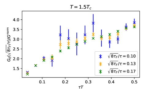
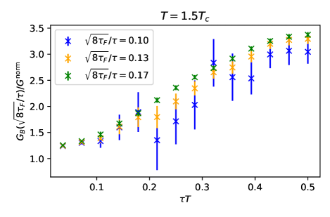
Figure 1: Normalized correlators $G_{\mathrm{E}}$ (top) and $G_{\mathrm{B}}$ (bottom) at fixed flow-time ratios, $\sqrt{8\tau_{\mathrm{F}}}/\tau$ for the $N_{t}=28$ lattice at $T=1.5T_{c}$. We see that with increasing ratio, the correlators converge toward a common shape across the whole $\tau T$ range.

In Fig. 1, we present both electric and magnetic correlators of the raw lattice data, normalized with Eq. (17) and tree-level improvement at different flow times for a single representative lattice size $N_{\rm t}=28$. We observe the statistical errors decreasing as the ratio $\sqrt{8\tau_{\mathrm{F}}}/\tau$ increases, and that for $\sqrt{8\tau_{\mathrm{F}}}/\tau>0.1$ the curves at different flow times seem to converge toward a common shape. This shape seems to be shared between both $G_{\mathrm{E}}$ and $G_{\mathrm{B}}$.

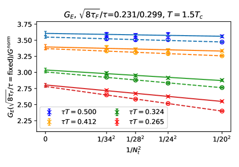
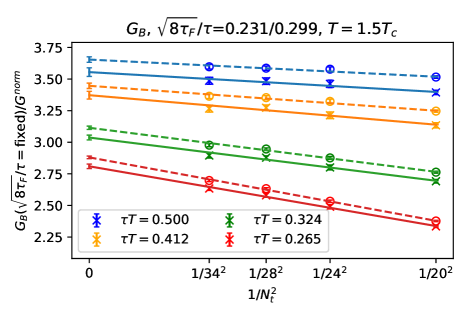
Figure 2: Examples of continuum extrapolations at fixed $\sqrt{8\tau_{\mathrm{F}}}/\tau$ for the chromoelectric (top) and chromomagnetic (bottom) correlators at $T=1.5T_{c}$. The dashed lines and circles indicate the limit taken at the lower edge of the flow-time ratio of interest $\sqrt{8\tau_{\mathrm{F}}}/\tau=0.231$ while solid lines and asterisks have a higher ratio of $\sqrt{8\tau_{\mathrm{F}}}/\tau=0.299$. The different $\tau T$ values are shown in different colors.

Next, we perform the continuum extrapolations of both correlators. First, we interpolate the data for each lattice in $\tau T$ at a fixed flow-time ratio with cubic spline interpolations. Since the correlators $G_{\mathrm{E},\mathrm{B}}$ are symmetric around the point $\tau T=0.5$, we set the first derivative of the splines equal to zero at $\tau T=0.5$. We perform a linear extrapolation in $1/N_{\rm t}^{2}=(aT)^{2}$ of the correlators at the fixed interpolated $\tau T$, and fixed flow-time ratio positions, using lattices $N_{\rm t}=20,~{}24,~{}28,~{}\mathrm{and}~{}34$ for large separations $\tau T>0.25$. For small separations $\tau T<0.25$, we drop the $N_{\rm t}=20$ lattice from the extrapolation. As an example, we show the continuum extrapolations at different $\tau T$ and $\sqrt{8\tau_{\mathrm{F}}}/\tau$ in Fig. 2. The $\chi^{2}/df$ of the continuum extrapolation is around 1 or smaller. For small $\tau$ some continuum extrapolations have large $\chi^{2}$, indicating that the cutoff effects are too large to obtain reliable results. We also perform continuum extrapolations including a $1/N_{\rm t}^{4}$ term for lattices with $N_{\rm t}=16$, which corresponds to a $\mathcal{O}(a^{4})$ continuum extrapolation. These continuum extrapolations agree with the ones shown in Fig. 2 within errors. Further details on the continuum extrapolations are discussed in Appendix A.

We present the continuum limits at the edges of the $\sqrt{8\tau_{\mathrm{F}}}/\tau$ range, within witch we will later take the zero-flow-time limit, and see that the continuum values vary less when $\sqrt{8\tau_{\mathrm{F}}}/\tau$ is changed than when $\tau T$ is changed. Hence, the thermal effects of heavy quark diffusion dominate the shape of these correlators.

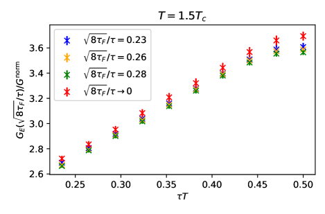
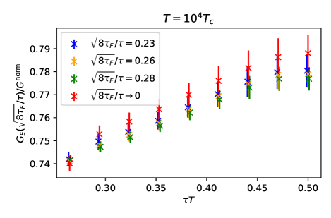
Figure 3: Continuum limit correlators of the chromoelectric correlator $G_{\mathrm{E}}$ at $T=1.5T_{c}$ (top) and $T=10^{4}T_{\rm c}$ (bottom) for different fixed flow-time ratios and in the zero-flow-time limit.

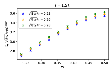
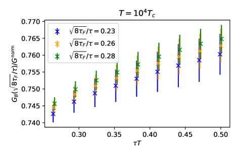
Figure 4: Continuum limit correlators of the chromomagnetic correlator $G_{\mathrm{B}}$ at $T=1.5T_{c}$ (top) and $T=10^{4}T_{\rm c}$ (bottom) for different fixed flow-time ratios.

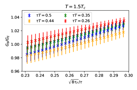
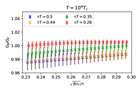
Figure 5: Ratio of the chromomagnetic to the chromoelectric correlator along the fixed flow-time ratio axis for temperatures $T=1.5T_{\rm c}$ (top) and $T=10^{4}T_{\rm c}$ (bottom).

Figures 3 and 4 show the final continuum limits of $G_{\mathrm{E}}$ and $G_{\mathrm{B}}$, respectively, for both measured temperatures as function of $\tau T$. Similarly to what we observed in Fig. 1, both correlators exhibit similar behavior at fixed temperatures according to the shape and order of magnitude. As mentioned above for the chromomagnetic correlator, we also perform calculations using clover discretizations and verify that the same continuum limit is obtained for this discretization. This is shown in Appendix A.

To further inspect this similarity, in Fig. 5 we plot the ratio $G_{\mathrm{E}}/G_{\mathrm{B}}$ along the fixed $\sqrt{8\tau_{\mathrm{F}}}/\tau$ axis, and observe a near-constant behavior toward large separations $\tau T$. From here, we can already deduce that the contribution to the heavy quark diffusion coefficient from the chromomagnetic correlator $G_{\mathrm{B}}$ is only going to differ from the contribution of the chromoelectric correlator $G_{\mathrm{E}}$ by less than 5%. In Fig. 3, we also show the zero-flow-time limit for the chromoelectric correlator $G_{\mathrm{E}}$, which will be discussed further in the next section.

III Measuring the diffusion coefficient on the lattice

III.1 Modeling of the spectral function

We now turn to extracting $\kappa_{\mathrm{E}}$ and $\kappa_{\mathrm{B}}$ from $G_{\mathrm{E}}$ and $G_{\mathrm{B}}$, respectively, using Eqs. (5) and (7). Our strategy for modeling the spectral function closely follows the approach laid out in our previous work Brambilla et al. (2020). This approach uses the perturbative information on the spectral function at large $\omega$, where this information is expected to be reliable. For both correlators, the spectral function $\rho_{\mathrm{E},\mathrm{B}}$ is known at the NLO level Burnier et al. (2010); Banerjee et al. (2022). We chose to model the spectral function such that in the UV regime at zero flow time it follows the $T=0$ part of the NLO spectral function; however, we chose the scale so that the NLO part vanishes, leaving us with only the LO part Caron-Huot et al. (2009):

$$\rho_{\mathrm{E},\mathrm{B}}^{\mathrm{LO}}(\omega,T)=\frac{g^{2}(\mu_{\omega}^{\mathrm{opt}})C_{\rm F}\omega^{3}}{6\pi}\,.$$ (22)

The coupling has been evaluated at the five-loop level in the $\overline{\textrm{MS}}$ scheme at the scale $\mu_{\omega}^{\mathrm{opt}}$, which for $\rho_{\mathrm{E}}$ reads Burnier et al. (2010),

$$\ln(\mu_{\omega})=\ln(2\omega)+\frac{(24\pi^{2}-149)}{66}\,.$$ (23)

For the electric spectral function $\rho_{\mathrm{E}}$, we further change to the NLO EQCD scale Kajantie et al. (1997)

$$\ln(\mu_{\omega})=\ln(4\pi T)-\gamma_{\mathrm{E}}-\frac{1}{22}$$ (24)

when $\omega\approx T$ or smaller. As we discuss below, the LO or NLO result for the UV part of the spectral function is not accurate, and we hence multiply it by a normalization factor $C_{n}$ to take into account higher-order corrections, i.e., we perform the replacement $\rho_{\mathrm{E},\mathrm{B}}^{\mathrm{LO}}\rightarrow C_{n}\rho_{\mathrm{E},\mathrm{B}}^{\mathrm{LO}}$. A similar normalization constant was used in the analysis of Refs. Francis et al. (2015a); Altenkort et al. (2021). The determination of $C_{n}$ is discussed at the end of this subsection. For $\rho_{\mathrm{E}}$, we do not model the flow-time dependence of the spectral function, as one is able to take the zero-flow-time limit before the spectral function inversion.

For the magnetic spectral function $\rho_{\mathrm{B}}$, the situation is more complicated due to the required renormalization Bouttefeux and Laine (2020); Laine (2021). In order to study the chromomagnetic correlator $G_{\mathrm{B}}$ at zero flow time, we use the relation between the UV part of $G_{B}$ at nonzero flow time and the corresponding renormalized correlator in the $\overline{\textrm{MS}}$ scheme:

$$G_{\mathrm{B}}^{\mathrm{flow,UV}}(\tau,\tau_{\mathrm{F}})= (1+\gamma_{0}g^{2}\ln(\mu\sqrt{8\tau_{\mathrm{F}}}))^{2}\times$$

$$Z_{\mathrm{flow}}G_{\mathrm{B}}^{\overline{\textrm{MS}},\mathrm{UV}}(\tau,\mu)+h_{0}\cdot(\tau_{\mathrm{F}}/\tau)\,,$$ (25)

where $h_{0}$ is a constant and $\gamma_{0}=3/(8\pi^{2})$ is the anomalous dimension of the chromomagnetic field Banerjee et al. (2022). In principle, the renormalization constant $Z_{\mathrm{flow}}$ can be calculated in perturbation theory; however, in practice we know from our previous calculation Brambilla et al. (2020) that the NLO perturbative results are not reliable enough to fully describe the lattice data. Hence, $Z_{\mathrm{flow}}$ is fixed by comparing the perturbative result to the lattice result on $G_{\mathrm{B}}$. Using the NLO result from Ref. Banerjee et al. (2022) and neglecting the distortions due to finite flow time (i.e., setting $h_{0}$ to zero), Eq. (25) gives a flow-time-dependent UV part of the chromomagnetic spectral density:

$$\rho_{\mathrm{B}}^{\mathrm{UV}}(\omega,\tau_{\mathrm{F}})= Z_{\mathrm{flow}}\frac{g^{2}(\mu)\omega^{3}}{6\pi}\times$$

$$(1+g^{2}(\mu)(\beta_{0}-\gamma_{0})\ln(\mu^{2}/(A\omega^{2}))$$

$$+g^{2}(\mu)\gamma_{0}\ln(8\tau_{\mathrm{F}}\mu^{2})\,,$$ (26)

where $\beta_{0}=11/(16\pi^{2})$ is the leading coefficient of the $\beta$ function, and

$$A=\exp\left[\frac{134}{35}-\frac{8\pi^{2}}{5}-\ln 4\right]\,.$$ (27)

As with $\rho_{\mathrm{E}}$, we choose the scale $\mu^{\mathrm{opt}}$ in such a way that Eqs. (26) and (22) are equal up to a constant, $Z_{\mathrm{flow}}$:

$$\mu^{\mathrm{opt}}=(\sqrt{A}\omega)^{1-\gamma_{0}/\beta_{0}}\cdot(8\tau_{\mathrm{F}})^{-\gamma_{0}/(2\beta_{0})}\,.$$ (28)

As in the case of the chromoelectric spectral function, here we make the replacement $\rho_{\mathrm{B}}^{\mathrm{UV}}\rightarrow C_{n}\rho_{\mathrm{B}}^{\mathrm{UV}}$ to take into account higher-order perturbative corrections. The determination of the normalization constant $C_{n}$ is discussed below, and now $C_{n}$ will also contain the unknown normalization factor $Z_{\mathrm{flow}}$.

The perturbative spectral functions described so far cover the UV regime of our model spectral functions. Alone, these UV spectral functions would give $\kappa_{\mathrm{E},\mathrm{B}}=0$, and hence an infrared contribution needs to be added leading to finite $\kappa_{\mathrm{E},\mathrm{B}}$. We note that while in general the chromomagnetic spectral function depends on the renormalization scheme ($\overline{\textrm{MS}}$, gradient flow, etc.) and scale, its low-frequency limit does not since $\kappa_{\mathrm{B}}$ is a physical quantity. This has been shown explicitly in weak-coupling calculations Bouttefeux and Laine (2020). One can work with the physical (RG-invariant) chromomagnetic spectral function by scaling out the anomalous dimension, or one can equally well work with the chromomagnetic correlation function in the gradient flow scheme at some finite, but sufficiently small, $\tau_{\mathrm{F}}$, and extract $\kappa_{\mathrm{B}}$.

In order to extract the $\kappa_{\mathrm{E},\mathrm{B}}$, we then follow the procedure laid out in our preceding study Brambilla et al. (2020) and model the spectral function with a family of Ansätze. For the large-$\omega$ regime in the UV, we assume the LO perturbative spectral function at $T=0$ as $\rho^{\mathrm{UV}}$ from Eq. (22) to hold. while for small $\omega$ in the IR, the spectral function is given by

$$\rho_{\mathrm{E},\mathrm{B}}^{\mathrm{IR}}(\omega,T)=\frac{\omega\kappa}{2T}\,.$$ (29)

We assume that $\rho_{\mathrm{E},\mathrm{B}}(\omega,T)=\rho^{\mathrm{IR}}(\omega,T)$ for $\omega<\omega^{\mathrm{IR}}$ and $\rho_{\mathrm{E},\mathrm{B}}(\omega,T)=\rho_{\mathrm{E},\mathrm{B}}^{\mathrm{UV}}(\omega,T)$ for $\omega>\omega^{\mathrm{UV}}$, where $\omega^{\mathrm{IR}}$ and $\omega^{\mathrm{UV}}$ are the limiting values of $\omega$ for which we can trust the above behaviors. In the region $\omega^{\mathrm{IR}}<\omega<\omega^{\mathrm{UV}}$, the form of the spectral function is generally not known, and this lack of knowledge will generate an uncertainty in the determination of $\kappa_{\mathrm{E},\mathrm{B}}$. Hence, for a given value of $\kappa_{\mathrm{E},\mathrm{B}}$, we construct the model spectral function that is given by $\rho_{\mathrm{E},\mathrm{B}}^{\mathrm{UV}}$ in $\omega>\omega^{\mathrm{UV}}$, $\rho_{\mathrm{E},\mathrm{B}}^{\mathrm{IR}}$ in $\omega<\omega^{\mathrm{IR}}$, and a variety of forms of $\rho_{\mathrm{E},\mathrm{B}}(\omega)$ for the intermediate $\omega^{\mathrm{IR}}\leq\omega\leq\omega^{\mathrm{UV}}$, such that the total spectral function is continuous. For the functional forms of the spectral function in the intermediate $\omega$ values, we consider two possible forms based on simple interpolations between the IR and UV regimes:

$$\rho_{\mathrm{E},\mathrm{B}}^{\mathrm{line}}(\omega,T)=\rho_{\mathrm{E},\mathrm{B}}^{\mathrm{IR}}(\omega,T)\theta(\omega^{\mathrm{IR}}-\omega)+$$

$$\left[\frac{\rho_{\mathrm{E},\mathrm{B}}^{\mathrm{IR}}(\omega^{\mathrm{IR}},T)-\rho_{\mathrm{E},\mathrm{B}}^{\mathrm{UV}}(\omega^{\mathrm{UV}},T)}{\omega^{\mathrm{IR}}-\omega^{\mathrm{UV}}}\left(\omega-\omega^{\mathrm{IR}}\right)+\rho_{\mathrm{E},\mathrm{B}}^{\mathrm{IR}}(\omega^{\mathrm{IR}},T)\right]$$

$$\times\theta(\omega-\omega^{\mathrm{IR}})\theta(\omega^{\mathrm{UV}}-\omega)+\rho_{\mathrm{E},\mathrm{B}}^{\mathrm{UV}}(\omega,T)\theta(\omega-\omega^{\mathrm{UV}})$$ (30)

and

$$\rho_{\mathrm{E},\mathrm{B}}^{\mathrm{step}}(\omega,T)=\rho_{\mathrm{E},\mathrm{B}}^{\mathrm{IR}}(\omega,T)\,\theta(\Lambda-\omega)+\rho_{\mathrm{E},\mathrm{B}}^{\mathrm{UV}}(\omega,T)\,\theta(\omega-\Lambda)\,,$$ (31)

where $\theta(\omega)$ is a step function. The case described in Eq. (31) corresponds to $\omega^{\mathrm{IR}}=\omega^{\mathrm{UV}}=\Lambda$ with the value of $\Lambda$ self-consistently determined, i.e., the value of $\Lambda$ is set by requiring the model spectral function to be continuous. We will refer to these two forms as the line model and the step model, respectively. In our previous analysis, we determined that the NLO spectral function takes the linear form for ${\omega<0.02T}$, and converges to the UV form at $\omega>2.2T$, and hence we use the same $\omega^{\mathrm{IR}}=0.01T$ and $\omega^{\mathrm{UV}}=2.2T$ as in Ref. Brambilla et al. (2020) for the line model (30) and for both chromomagnetic and chromoelectric spectral functions. The correlation functions obtained from the model spectral functions through Eq. (5) will be labeled as $G_{\mathrm{E},\mathrm{B}}^{\mathrm{model}}$.

The spectral representation of $G_{\mathrm{E},\mathrm{B}}$ given by Eq. (5) also holds at finite lattice spacing ($a\neq 0$) and finite flow time ($\tau_{\mathrm{F}}\neq 0$), as long as the spectral function $\rho_{\mathrm{E},\mathrm{B}}$ is replaced by a lattice equivalent $\rho_{\mathrm{E},\mathrm{B}}^{\mathrm{lat}}(a,\tau_{\mathrm{F}})$. The spectral function $\rho_{\mathrm{E},\mathrm{B}}^{\mathrm{lat}}(a,\tau_{\mathrm{F}})$ only has support for $\omega<\omega_{\mathrm{max}}$. In the case of meson correlators, a similar $\rho^{\mathrm{lat}}$ has been explicitly constructed in the free case Karsch et al. (2003). In this work, point-like meson sources and sinks are used. One often uses correlation functions of extended meson operators to improve the signal of the ground state. The spectral function of such extended meson correlators has also been calculated in the free theory Kaczmarek et al. (2004). It was found that for extended meson operators, the support of the spectral function shifts toward smaller $\omega$ values Kaczmarek et al. (2004), and their shape is modified at large $\omega$ but not at small $\omega$ Kaczmarek et al. (2004). The operators obtained from gradient flow can be viewed as extended operators, and therefore the shape of the corresponding spectral functions at large $\omega$ will be different compared to the unsmeared case, and the support of the spectral function will shift toward smaller $\omega$. However, the small-$\omega$ limit of $\rho_{\mathrm{E},\mathrm{B}}^{\mathrm{lat}}(a,\tau_{\mathrm{F}})$ will not depend on $a$ or $\tau_{\mathrm{F}}$ to a good approximation, because the correlator $G_{\mathrm{E},\mathrm{B}}$ is not sensitive to $a$ or $\tau_{\mathrm{F}}$, provided that $\tau\gg a$ and $\tau\gg\sqrt{8\tau_{\mathrm{F}}}$. Therefore, in principle, one can extract $\kappa_{\mathrm{E},\mathrm{B}}$ even at finite $a$ and $\tau_{\mathrm{F}}$. However, as this is valid only for $\omega<\omega_{\mathrm{max}}$, the large-$\omega$ part of $\rho_{\mathrm{E},\mathrm{B}}^{\mathrm{lat}}(a,\tau_{\mathrm{F}})$ cannot be described by the continuum perturbative result. We model the UV part of the spectral function $\rho_{\mathrm{E},\mathrm{B}}^{\mathrm{UV}}$ with Eq. (22), up to a multiplicative constant. The difference between these and the continuum spectral functions is not expected to be large in terms of the correlators $G_{\mathrm{E},\mathrm{B}}$ at $\tau T>0.25$, which is the relevant $\tau$ range for the determination of $\kappa_{\mathrm{E},\mathrm{B}}$.

The above statement about the dependence of the spectral function at large $\omega$ on the flow time appears to contradict the perturbative analysis of Ref. Altenkort et al. (2021). However, we note that in Ref. Altenkort et al. (2021) the analytic continuation was done in terms of the Matsubara frequency, while here we consider continuation in terms of $\tau$: $t\rightarrow-i\tau$. These two methods of analytic continuations lead to different results, unless the spectral function decays like $1/\omega^{2}$ for large $\omega$. Finally, we note that the cutoff effects in $\rho^{\mathrm{lat}}$ are not limited to the large-$\omega$ region. There are cutoff effects proportional to $(aT)^{2}\sim 1/N_{\rm t}^{2}$ which affect $\rho^{\mathrm{lat}}$ at all values of $\omega$. However, these are quite small for the $N_{\rm t}>16$ used in our calculations.

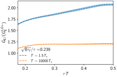
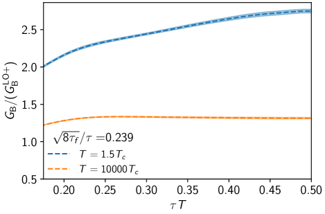
Figure 6: Chromoelectric (top) and the chromomagnetic (bottom) correlators normalized with the LO perturbative result, such that the running coupling is involved.

So far, we have presented the correlators $G_{\mathrm{E},\mathrm{B}}$ normalized with Eq. (17), which assumes a constant coupling. In Fig. 6 we include the running coupling in the analysis, and divide the continuum limit of the correlators for $\sqrt{8\tau_{\mathrm{F}}}/\tau=0.239$ with Eq. (5), using Eq. (22) with the scales (23) and (28) for $\rho_{\mathrm{E}}$ and $\rho_{\mathrm{B}}$, respectively. The corresponding correlators are labeled as $G_{\mathrm{E},\mathrm{B}}^{\mathrm{LO+}}$. We see from Fig. 6 that with this normalization the $\tau$ dependence of the corresponding ratios is greatly reduced. In particular, at the highest temperature $10^{4}T_{c}$, only very little $\tau$ dependence can be seen for $\tau T\geq 0.25$. The $\tau$ dependence observed for $\tau T<0.25$ is most likely due to the fact that our continuum extrapolation is not reliable at such small $\tau$ Brambilla et al. (2020). Thus, a large part of the $\tau$ dependence of $G_{\mathrm{E},\mathrm{B}}$ comes from the running of the coupling constant. On the other hand, the values of the ratios $G_{\mathrm{E},\mathrm{B}}/G_{\mathrm{E},\mathrm{B}}^{\mathrm{LO+}}$ differ significantly from one, even at relatively small $\tau$. A similar trend for $G_{\mathrm{E}}/G_{\mathrm{E}}^{\mathrm{LO+}}$ was observed in Ref. Brambilla et al. (2020). It was speculated in Ref. Brambilla et al. (2020) that the fact that $G_{\mathrm{E}}/G_{\mathrm{E}}^{\mathrm{LO+}}$ is roughly a constant that is different from one may be due to the one-loop renormalization of the lattice correlator not being reliable. However, as discussed in Sec. II.1, the one-loop renormalization of the chromoelectric correlator is quite reliable. This leads us to the conclusion that the NLO results for the spectral function may not be reliable and an additional normalization constant, $C_{n}$, has to be introduced as an extra fit parameter. The normalization constants $C_{n}$ are shown in Appendix B. For the chromoelectric correlator, the normalization constant $C_{n}$ is very close to the one obtained in our study using the multilevel algorithm Brambilla et al. (2020). In the case of the chromomagnetic correlator, the constant $C_{n}$ also contains the unknown matching between the gradient flow scheme and the $\overline{\textrm{MS}}$ scheme, as mentioned before. We suspect that the fact that the NLO result can describe the lattice correlators at small $\tau$ only up to a constant $C_{n}$ is due to the presence of the Wilson line and the Polyakov loop in the definition of the correlators. These do not contribute at order $g^{4}$, but will start contributing at higher orders. It is also known that the weak-coupling result for the Polyakov loop only works at temperatures $T>5$ GeV Bazavov et al. (2016). At higher orders, the presence of the Wilson line and the Polyakov loop most likely changes the overall normalization of the correlator, but not its $\tau$ dependence.

III.2 Flow time dependence of the correlators

To get rid of distortions due to gradient flow, the lattice results for $G_{\mathrm{E}}$ should be extrapolated to zero flow time. The limit to zero flow time has to be taken after the continuum limit to avoid the large discretization effects at small flow times. Also, it was argued in Refs. Altenkort et al. (2022); Eller (2021) that the inversion of the spectral function via Eq. (5) is mathematically well defined only in the zero-flow-time limit. As discussed in the previous subsection, it is possible to generalize the spectral representation in Eq. (5), for nonzero lattice spacing and flow time, if the corresponding spectral function only has support for $\omega$ values smaller than some $\omega_{\mathrm{max}}$.

We also note that in lattice studies of shear viscosity, spectral function inversion at finite flow time has given satisfactory results Mages et al. (2015); Itou and Nagai (2020). Moreover, in recent studies of latent heat, it has been observed that the order of the continuum and zero-flow-time limits can be switched as long as one is careful to only take the limits in regimes where the functional forms used are justified Shirogane et al. (2021). Therefore, we present our main analysis following the conventional order continuum limit $\rightarrow$ zero-flow-time limit $\rightarrow$ spectral function inversion for the main analysis, but we also present an analysis where these steps are taken in a different order.

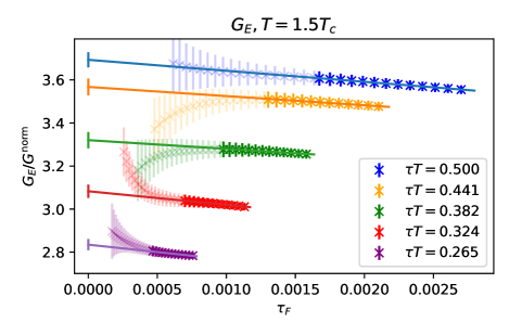
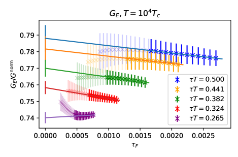
Figure 7: Final results of the continuum limits of the chromoelectric correlator $G_{\mathrm{E}}$ for both temperatures $T=1.5T_{\rm c}$ (top) and $T=10^{4}T_{\rm c}$ (bottom). The linear lines indicate the linear zero-flow-time limit. The dimmed symbols correspond to the data not used in the analysis.

To perform the extrapolation to the zero-flow-time limit, we use a linear ansatz in $\tau_{\mathrm{F}}$. A linear behavior is expected, as the small-$\tau_{\mathrm{F}}$ behavior is just a leading correction to the $\tau$ behavior due to flow. Moreover, for the chromoelectric correlator $G_{\mathrm{E}}$, the linear behavior has been seen at the NLO level of perturbation theory Eller (2021). Starting with the chromoelectric correlator $G_{\mathrm{E}}$, we present examples of linear zero-flow-time extrapolations at a few chosen $\tau T$ values in Fig. 7. As expected, we see a clear linear dependence in the range where the extrapolation can be performed. We observe that the correlator $G_{\mathrm{E}}$ decreases with increasing flow time. The whole range of $\tau T$ dependence of the zero-flow-time results was already presented in Fig. 3. As one can see from that figure, the flow-time dependence is not very large in the considered flow-time window. In particular, the shape of the correlator does not change significantly with the flow time and it is very similar to the shape of the correlator extrapolated to zero flow time. Thus, the determination of $\kappa_{E}$ is not significantly affected by the nonzero flow time. Therefore, one can also model the spectral function corresponding to nonzero flow time and determine $\kappa_{\mathrm{E}}$. The effects of the small residual distortion of the correlator due to gradient flow on $\kappa_{\mathrm{E}}$ can be taken care of by performing a zero-flow-time extrapolation for the resulting $\kappa_{\mathrm{E}}$. This analysis strategy will be discussed in the next subsection.

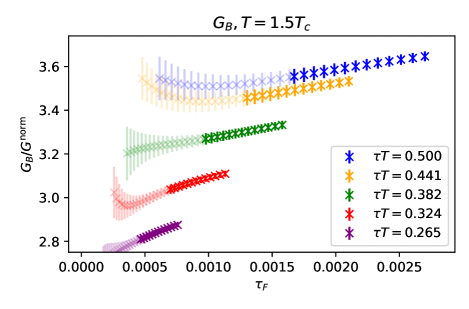
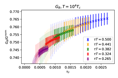
Figure 8: Final results of the continuum limits of the chromomagnetic correlators for both temperatures: $T=1.5T_{\rm c}$ (top) and $T=10^{4}T_{\rm c}$ (bottom). The dimmed symbols correspond to the lattice data not used in the determination of $\kappa_{\mathrm{B}}$.

The flow-time dependence of the chromomagnetic correlator is shown in Fig. 8, and appears to be quite different from the flow-time dependence of the chromoelectric correlator. The flow time dependence of $G_{\mathrm{B}}$ appears to be roughly linear, but its slope has the opposite sign. This difference is expected and probably comes from the nontrivial renormalization of $G_{\mathrm{B}}$, cf. Eq. (25). This renormalization is taken care of at leading-order in $G_{\mathrm{B}}^{\mathrm{LO+}}$. Normalizing the chromomagnetic correlator by $G_{\mathrm{B}}^{\mathrm{LO+}}$, instead of by $G^{\rm norm}$, largely reduces the flow-time dependence. This is shown in Fig. 9. In the case of the chromomagnetic correlator we do not take the zero-flow-time limit, but instead model the spectral function for nonzero flow time using Eqs. (26), (29), (30), and (31), and then perform the zero-flow-time extrapolation of $\kappa_{\mathrm{B}}$ obtained from this modeling, as will be described below.

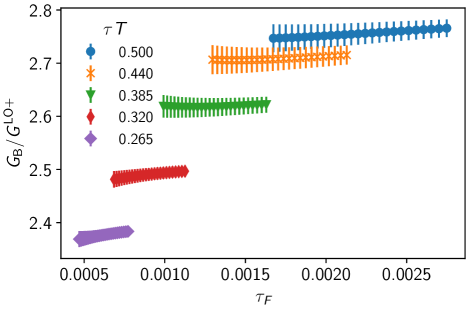
Figure 9: Continuum limit correlators of the chromomagnetic correlator $G_{\mathrm{B}}$ at $T=1.5T_{\rm c}$ divided by our default UV model for the spectral function $\rho_{\mathrm{B}}$ as functions of flow time for a few representative values of $\tau T$.

III.3 Results: $\kappa_{\mathrm{E}}$

The extraction of $\kappa_{\mathrm{E}}$ proceeds as follows. We take the continuum and zero-flow-time limit data and perform a least-squares fit to Eq. (5) with either of the models of the spectral function $\rho_{\mathrm{E},\mathrm{B}}(\omega)$. In addition to having $\kappa_{\mathrm{E},\mathrm{B}}$ as a fit parameter, we also enforce a normalization in the fit by finding a normalization coefficient $C_{n}(\tau_{\mathrm{min}}T)$ fit parameter such that $G_{\mathrm{E}}(\tau_{\mathrm{min}}T)/G_{\mathrm{E}}^{\mathrm{model}}(\tau_{\mathrm{min}}T)=1$. To estimate the contributions from the systematic errors, we perform these fits with different values of $\tau T_{\mathrm{min}}$, vary the scale $\mu$ of the running coupling by a factor of 2, and perform the fit with either the line (30) or step (31) models of the spectral function. To get the final estimate for the heavy quark momentum diffusion coefficient, we then take the full spread of the subset of these fits for which the ratio $G_{\mathrm{E}}(\tau T>\tau_{\mathrm{min}}T)/G_{\mathrm{E}}^{\mathrm{model}}(\tau T>\tau_{\mathrm{min}}T)=1$ is within $1.5\sigma$.

For the $G_{\mathrm{E}}$ data, which was first extrapolated to the continuum limit and then to the zero-flow-time limit, this procedure gives for $\kappa_{\mathrm{E}}$

$$1.70\leq\frac{\kappa_{\mathrm{E}}}{T^{3}}\leq 3.12$$ (32)

at $T=1.5T_{\rm c}$ and

$$0.02\leq\frac{\kappa_{\mathrm{E}}}{T^{3}}\leq 0.16$$ (33)

at $T=10^{4}T_{\rm c}$. The $T=1.5T_{\rm c}$ result gives a slightly improved range for $\kappa_{\mathrm{E}}$ compared to our previous multilevel study Brambilla et al. (2020), which had $1.31<\kappa_{\mathrm{E}}/T^{3}<3.64$. Although slightly smaller, it is also in agreement with the other existing results for this temperature: $2.31<\kappa_{\mathrm{E}}/T^{3}<3.70$ from Ref. Altenkort et al. (2022), $1.8<\kappa_{\mathrm{E}}/T^{3}<3.4$ from Ref. Francis et al. (2015a), $1.55<\kappa_{\mathrm{E}}/T^{3}<3.95$ from Ref. Banerjee et al. (2012), and $1.3<\kappa_{\mathrm{E}}/T^{3}<2.8$ from Ref. Banerjee et al. (2022). The $T=10^{4}T_{\rm c}$ result is in agreement with our previous result $0<\kappa_{\mathrm{E}}/T^{3}<0.1$ Brambilla et al. (2020). The new result has slightly larger errors due to the gradient flow analysis having more strict fit regimes; however, we can for the first time observe a nonzero minimum for $\kappa_{\mathrm{E}}/T^{3}$ at very large temperature. Both of these $\kappa_{\mathrm{E}}$ values can be reexpressed as a position-space momentum diffusion coefficient $D_{\mathrm{s}}=2T^{2}/\kappa$ Caron-Huot et al. (2009) as: $0.64<D_{\mathrm{s}}T<1.17$ for $T=1.5T_{\rm c}$ and $12.5<D_{\mathrm{s}}T<100$ for $T=10^{4}T_{\rm c}$.

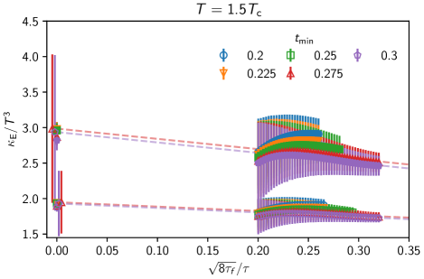
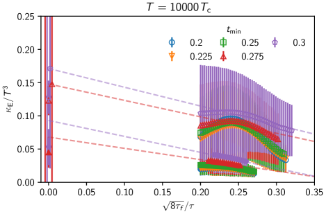
Figure 10: Heavy quark momentum diffusion coefficient $\kappa_{\mathrm{E}}/T^{3}$ at different flow-time ratios $\sqrt{8\tau_{\mathrm{F}}}/\tau$ for both temperatures $T=1.5T_{\rm c}$ (top) and $T=10^{4}T_{\rm c}$ (bottom). The filled symbols are from the extraction using the line ansatz (30) and the empty symbols are from the step ansatz (31) of the spectral function. Different colors depict the different choices for the normalization point $\tau T_{\mathrm{min}}$. For large $\tau T_{\mathrm{min}}\geq 0.275$ it is possible to perform linear extrapolation to zero flow time, which is shown as faint dashed lines in color equivalent to the respective $\tau T_{\mathrm{min}}$.

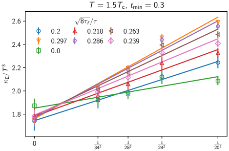
Figure 11: Heavy quark momentum diffusion coefficient $\kappa_{\mathrm{E}}/T^{3}$ extracted at finite lattice spacing for different flow-time ratios $\sqrt{8\tau_{\mathrm{F}}}/\tau$ shown with different colors and symbols, for a representative case for $T=1.5T_{\rm c}$ and $\tau T_{\mathrm{min}}=0.3$.

We now turn to a question of how the result for $\kappa_{\mathrm{E}}$ depends on the order of the limits. First, in Fig. 10 we show the extracted values of $\kappa_{\mathrm{E}}/T^{3}$ both at the zero-flow-time limit and at a finite flow time for both the line (30) (filled symbols) and the step (31) (empty symbols) models for the spectral function $\rho(\omega)$. Only points that are within the regime $0.2<\sqrt{8\tau_{\mathrm{F}}}/\tau<0.3$ where reasonable zero-flow-time extrapolation can be performed and that satisfy the condition $G_{\mathrm{E}}(\tau T>\tau T_{\mathrm{min}})/G_{\mathrm{E}}^{\mathrm{model}}(\tau T>\tau T_{\mathrm{min}})=1$ within $1.5\sigma$ are shown. In addition, we show in different colors the different choices of the normalization point $\tau T_{\mathrm{min}}$. We observe that the variation between the models is the dominant source of error and that the variation within the flow time is small in comparison. Moreover, with reasonably high $\tau T_{\mathrm{min}}\geq 0.275$, we have enough data points to perform a linear zero-flow-time extrapolation, which we can see agrees closely with the results we get from data that has been extrapolated to zero flow time before spectral function inversion, although with much larger errors. If we were to do the $\kappa_{\mathrm{E}}$ extraction purely at finite flow time, the full variance due to the different fit forms would give us $1.5\leq\frac{\kappa_{\mathrm{E}}}{T^{3}}\leq 3.2$ for $T=1.5T_{\rm c}$ and $0.007\leq\kappa_{\mathrm{E}}/T^{3}\leq 0.18$ for $T=10^{4}T_{\rm c}$. Therefore, the variance for a given finite flow time is much larger than the difference between the continuum extrapolated $\kappa_{\mathrm{E}}$ extractions.

Furthermore, we inspect whether it matters that the continuum limit is taken before everything else, as has been done so far. If we were to instead extract the $\kappa_{\mathrm{E}}$ at finite lattice spacing and then take the continuum limit as a linear extrapolation of the extracted $\kappa_{\mathrm{E}}$ values, we would get the result in Fig. 11. We see that the continuum limit of the $\kappa_{\mathrm{E}}$ extracted at finite lattice spacing replicates both the zero-flow-time result, and the results at finite ratio $\sqrt{8\tau_{\mathrm{F}}}/\tau$. Hence, all results presented above would remain unchanged even if the continuum limit had been taken last, because of the large uncertainties in $\kappa_{\mathrm{E}}$ due to the modeling of the spectral function.

III.4 Results: $\kappa_{\mathrm{B}}$

We now turn to the chromomagnetic correlator $G_{\mathrm{B}}$ and extraction of the respective $\kappa_{\mathrm{B}}$. Based on the above analysis for $\kappa_{\mathrm{E}}$, we can safely assume that one can get a very good estimate of the zero-flow-time-extrapolated value even when limiting the analysis to a finite flow time. Our analysis strategy here closely follows the case of the chromoelectric correlator. First, we fix the normalization constant $C_{n}$ and then vary $\kappa_{\mathrm{B}}$ to obtain the best agreement of the lattice correlator with the model correlator. To demonstrate this point for the step Ansatz, we write

$$\displaystyle G_{\mathrm{B}}^{\rm model}=\frac{\kappa_{\mathrm{B}}}{2T}\int_{0}^{\Lambda_{T}}\frac{\mathop{\mathrm{d}\omega}}{\pi}\omega K(\omega,\tau T)+$$

$$\displaystyle C_{n}(\tau_{\mathrm{F}})\int_{\Lambda_{T}}^{\infty}\frac{d\omega}{\pi}\frac{C_{\rm F}g^{2}(\mu_{\omega})}{6\pi}\omega^{3}K(\omega,\tau T)\,,$$ (34)

where $\Lambda_{T}\sim T$ is some IR cutoff. We treat $\kappa_{\mathrm{B}}$ as a fit parameter, while $C_{n}(\tau_{F})$ is adjusted such that $G_{\mathrm{B}}^{\rm model}$ from the above equation exactly matches the continuum lattice result for $G_{\mathrm{B}}$ at $\tau=\tau_{\rm min}$. The values of $C_{n}$ are shown in Appendix B as a function of $\tau_{\mathrm{F}}$. In Fig. 12 we show the spectral function corresponding to the chromomagnetic correlators for $\sqrt{8\tau_{\mathrm{F}}}/\tau=0.25$ and $0.3$. As one can see from the figure, the flow-time dependence of the spectral function is rather mild.

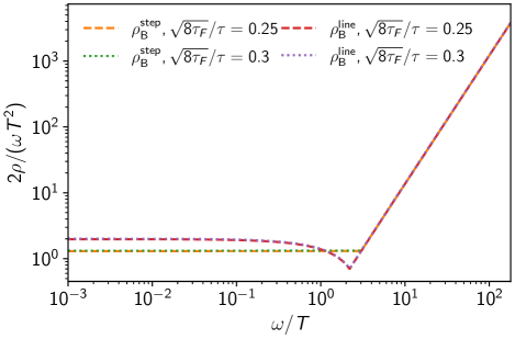
Figure 12: Spectral function of chromomagnetic correlators obtained from the two fit forms described in the text at two different representative flow-time ratios. Only the mean value is shown and the statistical errors are hidden for better visibility.

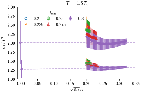
Figure 13: Magnetic heavy quark momentum diffusion coefficient $\kappa_{\mathrm{B}}/T^{3}$ at different flow-time ratios $\sqrt{8\tau_{\mathrm{F}}}/\tau$ for $T=1.5T_{\rm c}$. The filled symbols are from extraction using the line ansatz (30) and the empty symbols are from the step ansatz (31) of the spectral function. Different colors depict the different choice for the normalization point $\tau T_{\mathrm{min}}$. The lines and points at $\sqrt{8\tau_{\mathrm{F}}}/\tau=0$ depict the zero-flow-time limit taken in the regime $\sqrt{8\tau_{\mathrm{F}}}/\tau\geq 0.25$.

The flow time behavior of the extracted $\kappa_{\mathrm{B}}/T^{3}$ is shown in Fig. 13, where again the filled symbols show the extraction using the line ansatz (30), the empty symbols show the extraction with the step model (31), and different colors depict the different choices of $\tau T_{\mathrm{min}}$. We observe less curvature in the extracted $\kappa_{\mathrm{B}}$ values than we saw for $\kappa_{\mathrm{E}}$ in Fig. 10. If we take the total variation at finite flow time to be the error of $\kappa_{\mathrm{B}}$, we get for $T=1.5T_{\rm c}$ that $1.23<\kappa_{\mathrm{B}}/T^{3}<2.74$. We can then proceed to take the zero-flow-time limit in the linear regime $\sqrt{8\tau_{\mathrm{F}}}/\tau\geq 0.25$, similar to what we learned to work with in the case of $G_{\mathrm{E}}$. In the zero-flow-time limit, we get the final result for $\kappa_{\mathrm{B}}$:

$$1.03\leq\frac{\kappa_{\mathrm{B}}}{T^{3}}\leq 2.61\,.$$ (35)

This result is well in agreement with the recent result Banerjee et al. (2022) of $1.0\leq\kappa_{\mathrm{B}}/T^{3}\leq 2.1$. The current data is not accurate enough to determine $\kappa_{\mathrm{B}}$ at $T=10^{4}T_{c}$.

IV Conclusions

In this paper, we have studied the chromoelectric and chromomagnetic correlators in quenched QCD with the aim to determine the heavy quark diffusion coefficient, including the subleading correction in the inverse quark mass. We used gradient flow for noise reduction and showed how to control the distortions due to nonzero flow time in the calculations of the transport coefficients $\kappa_{\mathrm{E}}$ and $\kappa_{\mathrm{B}}$. To obtain the heavy quark diffusion coefficient, we used a parametrization of the spectral functions that relies on the NLO result at large energies, and smoothly matched to the expected linear behavior at small energies. The effects of the nonzero flow time can be incorporated into the high energy part of the spectral function. We verified this in the calculations of $\kappa_{\mathrm{E}}$, where we obtained $\kappa_{\mathrm{E}}$ from the chromoelectric correlator extrapolated to zero flow time, as well as by calculating an effective $\kappa_{\mathrm{E}}$ from the chromoelectric correlator at finite flow time and then extrapolating to zero flow time. Our main results are summarized in Eqs. (32), (33) and (35). Our results for $\kappa_{\mathrm{E}}$ agree with the previous determinations Kaczmarek (2014); Brambilla et al. (2020); Altenkort et al. (2022) within the estimated uncertainties. The value of $\kappa_{\mathrm{B}}$ we obtained agrees with the very recent result obtained using the multilevel algorithm and nonperturbative renormalization based on the Schrödinger functional Banerjee et al. (2022). We have seen that the dominant uncertainty in the determination of $\kappa_{\mathrm{E}}$ and $\kappa_{\mathrm{B}}$ comes from the modeling of the spectral functions at low energies. Using the lattice results for $\langle\mathbf{v}^{2}\rangle$ from Ref. Petreczky (2009) for charm and bottom quarks $\langle\mathbf{v}^{2}\rangle_{\mathrm{charm}}\simeq 0.51$ and $\langle\mathbf{v}^{2}\rangle_{\mathrm{bottom}}\simeq 0.3$ (c.f. Fig. 6 of Ref. Petreczky (2009) where $v_{th}^{2}=\langle\mathbf{v}^{2}\rangle/3$ was shown), we estimate that the mass-suppressed effect on the heavy quark diffusion coefficient is 34% and 20% for charm and bottom quarks, respectively.

The extraction of the heavy quark diffusion constant strongly relies on using the NLO result for the spectral function at large energies. It is assumed that the NLO result can describe the $\tau$ dependence of the correlators up to a multiplicative constant. To test this assertion further, it would be desirable to perform calculations at larger $N_{\tau}$, so that reliable continuum extrapolations are possible for smaller values of $\tau$. Another way to obtain more reliable continuum-extrapolated results is to use the Symanzik-improved gauge action. We plan to implement such an improved analysis in the near future. Finally, once the full one-loop perturbative matching between the $\overline{\textrm{MS}}$ scheme and the gradient flow scheme at small flow times becomes available, we will redo our analysis by converting to the $\overline{\textrm{MS}}$ scheme and taking the zero-flow-time limit.

Appendix A Discretization effects and continuum extrapolations

In this appendix, we discuss discretization effects and continuum extrapolations in more detail. In Fig. 14 we show different continuum extrapolations for the chromoelectric correlators as a function of $\tau$ for a few representative values of the flow time. We perform extrapolations assuming a $1/N_{\rm t}^{2}$ form for the discretization errors and vary the range in $N_{\rm t}$, and also include a $1/N_{\rm t}^{4}$ term in the continuum extrapolations with $N_{\rm t}=16$ lattices. For $\tau T>0.25$ different continuum extrapolations agree well with each other.

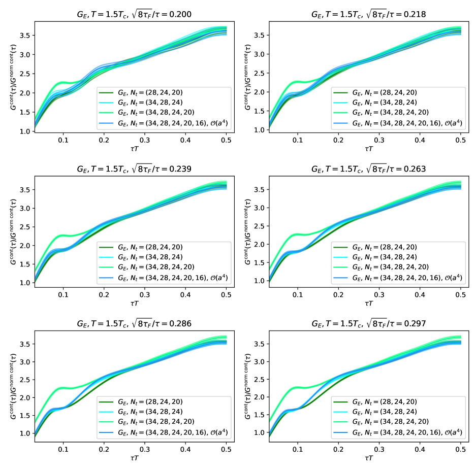
Figure 14: Chromoelectric correlator with different continuum extrapolations for some representative flow times.

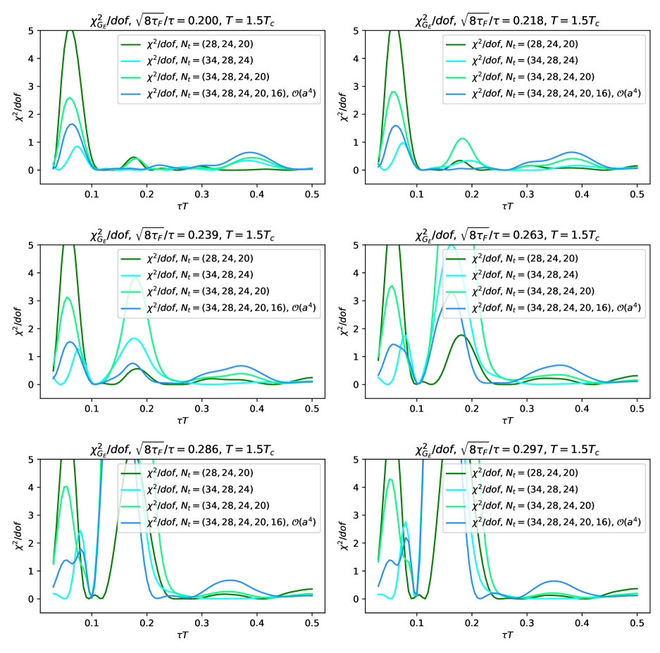
Figure 15: $\chi^{2}/df$ of different continuum extrapolations of the chromoelectric correlators for some representative flow times.

The $\chi^{2}/df$ of the continuum extrapolations are shown in Fig. 15. For $\tau T>0.25$, different continuum extrapolations of the chromoelectric correlators agree well, and the $\chi^{2}/df$ of the continuum extrapolation is close to one or smaller. For smaller $\tau T$ the $\chi^{2}/df$ is large, indicating that the continuum extrapolations are not reliable. We perform a similar analysis for the chromomagnetic correlators. Some results are shown in Fig. 16

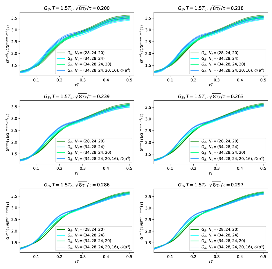
Figure 16: Chromomagnetic correlator with different continuum extrapolations for some representative flow times.

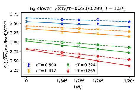
Figure 17: Continuum extrapolation of the chromomagnetic correlator with the clover discretization and the corresponding tree-level improvement (36). The results are shown for two different flow times indicated in the label of the figure.

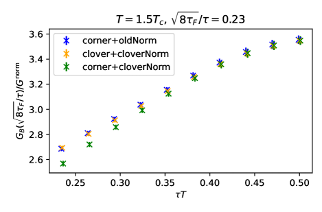
Figure 18: We compare the results of the continuum limits for the following three cases: the corner discretization (4) normalized with Eq. (17) (corner+cornerNorm), the clover discretization normalized with Eq. (36) (clover+cloverNorm), the and corner discretization normalized with Eq. (36) (corner+cloverNorm).

As discussed in the main text for the chromomagnetic correlators, we use two discretization schemes: the simplest one given by Eq. (4), which can be labeled as the corner discretization, and the clover discretization which was also used in Ref. Banerjee et al. (2022) (c.f. Eqs. (2.2)-(2.4) herein). These two discretizations must agree in the continuum, but could lead to quite different result at nonzero lattice spacings. As a result, the tree-level improvements for these two discretization schemes are also different. The leading-order result for the clover discretization without the $g^{2}$ and $C_{F}$ factors has the form

$$G_{\mathrm{norm}}^{\mathrm{Latt}}(\tau)=\frac{1}{3a^{4}}\int_{-\pi}^{\pi} \frac{\mathrm{d}^{3}\mathbf{q}}{(2\pi)^{3}}\frac{e^{\bar{q}N_{t}(1-\tau T)}+e^{\bar{q}N_{t}\tau T}}{e^{\bar{q}N_{t}}-1}$$

$$\times\frac{\tilde{q}-\frac{(\tilde{q}^{2})^{2}+\tilde{q}^{4}}{8}+\frac{\tilde{q}^{2}\tilde{q}^{4}-\tilde{q}^{6}}{32}}{\sinh\bar{q}},$$ (36)

where $\bar{q}$ and $\tilde{q}$ are given by Eqs. (19) and (20) respectively. We use this to implement the tree level improvement for the clover discretization scheme. In Fig. 17 we show the continuum limit of the flowed chromomagnetic correlator with the clover discretization and the tree-level improvement (36). We show results for two different flow times, for which the expected $1/N_{\rm t}^{2}$ behavior can be clearly seen in the lattice data in both cases. We also compare the continuum extrapolated results obtained with the corner and clover discretizations, and the corresponding tree-level improvements, in Fig. 18. As one can see from the figures, the continuum results obtained with the two discretization schemes are in excellent agreement. The tree-level improvement reduces the discretization effects and therefore, aids robust continuum extrapolations. However, as discussed in Ref. Brambilla et al. (2020) it is not necessary if the lattice spacing is sufficiently small or, equivalently, if $N_{\rm t}$ is large enough. Small lattice spacings are needed for reliable continuum extrapolation at small $\tau T$. If $\tau T$ is not very small, the continuum extrapolation can be performed without tree-level improvement Brambilla et al. (2020). To check to what extent our conclusions on the continuum result of the chromomagnetic correlator depend on the tree-level improvement, we perform continuum extrapolations of the chromomagnetic correlator with the corner discretization scheme but using the "wrong" tree-level improvement, namely, the tree-level improvement for the clover discretization. The corresponding continuum results are also shown in Fig. 18 and labeled as "corner+cloverNorm". For $\tau T<0.35$ we see small, but statistically significant, differences compared to the continuum results obtained with proper tree-level improvement, but for larger values of $\tau T$ the tree-level improvement is not essential for reliable continuum extrapolations.

Appendix B Normalization parameter

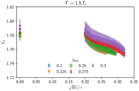
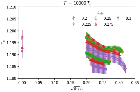
Figure 19: Normalization coefficient $C_{n}$ for the chromoelectric correlator $G_{\mathrm{E}}$ at different flow-time ratios $\sqrt{8\tau_{\mathrm{F}}}/\tau$ for both temperatures $T=1.5T_{\rm c}$ (top) and $T=10^{4}T_{\rm c}$ (bottom). The filled symbols are from extraction using the line ansatz (30) and the empty symbols are from the step ansatz (31) of the spectral function. Different colors depict the different choice for the normalization point $\tau T_{\mathrm{min}}$.

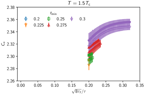
Figure 20: Normalization coefficient $C_{n}$ for the chromomagnetic correlator $G_{\mathrm{B}}$ at different flow-time ratios $\sqrt{8\tau_{\mathrm{F}}}/\tau$ for the temperature $T=1.5T_{\rm c}$. The filled symbols are from extraction using the line ansatz (30) and the empty symbols are from the step ansatz (31) of the spectral function. Different colors depict the different choice for the normalization point $\tau T_{\mathrm{min}}$.

For completeness, we also show in Figs. 19 and 20 the normalization coefficient $C_{n}$ for both $G_{\mathrm{E}}$ and $G_{\mathrm{B}}$ respectively. We observe that $C_{n}$ has a very mild dependence on the flow time. This can be used as an indication that modeling $\rho_{\mathrm{E},\mathrm{B}}^{\mathrm{lat}}$ with the running coupling version of the leading-order $\rho_{\mathrm{E},\mathrm{B}}$ is reasonably well motivated. The $C_{n}$ values for the chromoelectric correlator are well in agreement with the ones we reported in our preceding study Brambilla et al. (2020): $\sim 1.73$ for $T=1.5T_{\rm c}$ and $\sim 1.2$ for $T=10^{4}T_{\rm c}$. The $C_{n}$ for the chromomagnetic field is slightly larger than the respective factor for $G_{\mathrm{E}}$.

References

- Moore and Teaney (2005) Guy D. Moore and Derek Teaney, “How much do heavy quarks thermalize in a heavy ion collision?” Phys. Rev. C71, 064904 (2005), arXiv:hep-ph/0412346 [hep-ph] .
- Svetitsky (1988) B. Svetitsky, “Diffusion of charmed quarks in the quark-gluon plasma,” Phys. Rev. D37, 2484–2491 (1988).
- Caron-Huot and Moore (2008) Simon Caron-Huot and Guy D. Moore, “Heavy quark diffusion in QCD and N=4 SYM at next-to-leading order,” JHEP 02, 081 (2008), arXiv:0801.2173 [hep-ph] .
- Bouttefeux and Laine (2020) A. Bouttefeux and M. Laine, “Mass-suppressed effects in heavy quark diffusion,” JHEP 12, 150 (2020), arXiv:2010.07316 [hep-ph] .
- Laine (2021) M. Laine, “1-loop matching of a thermal Lorentz force,” JHEP 06, 139 (2021), arXiv:2103.14270 [hep-ph] .
- Brambilla et al. (2017) Nora Brambilla, Miguel A. Escobedo, Joan Soto, and Antonio Vairo, “Quarkonium suppression in heavy-ion collisions: an open quantum system approach,” Phys. Rev. D96, 034021 (2017), arXiv:1612.07248 [hep-ph] .
- Brambilla et al. (2018) Nora Brambilla, Miguel A. Escobedo, Joan Soto, and Antonio Vairo, “Heavy quarkonium suppression in a fireball,” Phys. Rev. D97, 074009 (2018), arXiv:1711.04515 [hep-ph] .
- Brambilla et al. (2019) Nora Brambilla, Miguel A. Escobedo, Antonio Vairo, and Peter Vander Griend, “Transport coefficients from in medium quarkonium dynamics,” Phys. Rev. D100, 054025 (2019), arXiv:1903.08063 [hep-ph] .
- Herzog et al. (2006) C. P. Herzog, A. Karch, P. Kovtun, C. Kozcaz, and L. G. Yaffe, “Energy loss of a heavy quark moving through N=4 supersymmetric Yang-Mills plasma,” JHEP 07, 013 (2006), arXiv:hep-th/0605158 [hep-th] .
- Casalderrey-Solana and Teaney (2006) Jorge Casalderrey-Solana and Derek Teaney, “Heavy quark diffusion in strongly coupled N=4 Yang-Mills,” Phys. Rev. D 74, 085012 (2006), arXiv:hep-ph/0605199 .
- Petreczky and Teaney (2006) Peter Petreczky and Derek Teaney, “Heavy quark diffusion from the lattice,” Phys. Rev. D73, 014508 (2006), arXiv:hep-ph/0507318 [hep-ph] .
- Aarts and Martinez Resco (2002) Gert Aarts and Jose Maria Martinez Resco, “Transport coefficients, spectral functions and the lattice,” JHEP 04, 053 (2002), arXiv:hep-ph/0203177 [hep-ph] .
- Petreczky (2009) P. Petreczky, “On temperature dependence of quarkonium correlators,” Eur. Phys. J. C 62, 85–93 (2009), arXiv:0810.0258 [hep-lat] .
- Ding et al. (2012) H. T. Ding, A. Francis, O. Kaczmarek, F. Karsch, H. Satz, and W. Soeldner, “Charmonium properties in hot quenched lattice QCD,” Phys. Rev. D86, 014509 (2012), arXiv:1204.4945 [hep-lat] .
- Borsanyi et al. (2014) Szabolcs Borsanyi et al., “Charmonium spectral functions from 2+1 flavour lattice QCD,” JHEP 04, 132 (2014), arXiv:1401.5940 [hep-lat] .
- Ding et al. (2021) Heng-Tong Ding, Olaf Kaczmarek, Anna-Lena Lorenz, Hiroshi Ohno, Hauke Sandmeyer, and Hai-Tao Shu, “Charm and beauty in the deconfined plasma from quenched lattice QCD,” Phys. Rev. D 104, 114508 (2021), arXiv:2108.13693 [hep-lat] .
- Caron-Huot et al. (2009) Simon Caron-Huot, Mikko Laine, and Guy D. Moore, “A Way to estimate the heavy quark thermalization rate from the lattice,” JHEP 04, 053 (2009), arXiv:0901.1195 [hep-lat] .
- Meyer (2011) Harvey B. Meyer, “The errant life of a heavy quark in the quark-gluon plasma,” New J. Phys. 13, 035008 (2011), arXiv:1012.0234 [hep-lat] .
- Francis et al. (2011) A. Francis, O. Kaczmarek, M. Laine, and J. Langelage, “Towards a non-perturbative measurement of the heavy quark momentum diffusion coefficient,” Proceedings, 29th International Symposium on Lattice field theory (Lattice 2011): Squaw Valley, Lake Tahoe, USA, July 10-16, 2011, PoS LATTICE2011, 202 (2011), arXiv:1109.3941 [hep-lat] .
- Banerjee et al. (2012) Debasish Banerjee, Saumen Datta, Rajiv Gavai, and Pushan Majumdar, “Heavy Quark Momentum Diffusion Coefficient from Lattice QCD,” Phys. Rev. D85, 014510 (2012), arXiv:1109.5738 [hep-lat] .
- Francis et al. (2015a) A. Francis, O. Kaczmarek, M. Laine, T. Neuhaus, and H. Ohno, “Nonperturbative estimate of the heavy quark momentum diffusion coefficient,” Phys. Rev. D92, 116003 (2015a), arXiv:1508.04543 [hep-lat] .
- Brambilla et al. (2020) Nora Brambilla, Viljami Leino, Peter Petreczky, and Antonio Vairo, “Lattice QCD constraints on the heavy quark diffusion coefficient,” Phys. Rev. D 102, 074503 (2020), arXiv:2007.10078 [hep-lat] .
- Lüscher and Weisz (2001) Martin Lüscher and Peter Weisz, “Locality and exponential error reduction in numerical lattice gauge theory,” JHEP 09, 010 (2001), arXiv:hep-lat/0108014 [hep-lat] .
- Boguslavski et al. (2021) K. Boguslavski, A. Kurkela, T. Lappi, and J. Peuron, “Heavy quark momentum diffusion coefficient in 3D gluon plasma,” Nucl. Phys. A 1005, 121970 (2021), arXiv:2001.11863 [hep-ph] .
- Boguslavski et al. (2020) K. Boguslavski, A. Kurkela, T. Lappi, and J. Peuron, “Heavy quark diffusion in an overoccupied gluon plasma,” JHEP 09, 077 (2020), arXiv:2005.02418 [hep-ph] .
- Banerjee et al. (2022) D. Banerjee, S. Datta, and M. Laine, “Lattice study of a magnetic contribution to heavy quark momentum diffusion,” JHEP 08, 128 (2022), arXiv:2204.14075 [hep-lat] .
- Narayanan and Neuberger (2006) R. Narayanan and H. Neuberger, “Infinite N phase transitions in continuum Wilson loop operators,” JHEP 03, 064 (2006), arXiv:hep-th/0601210 .
- Lüscher (2010a) Martin Lüscher, “Trivializing maps, the Wilson flow and the HMC algorithm,” Commun. Math. Phys. 293, 899–919 (2010a), arXiv:0907.5491 [hep-lat] .
- Lüscher (2010b) Martin Lüscher, “Properties and uses of the Wilson flow in lattice QCD,” JHEP 08, 071 (2010b), [Erratum: JHEP 03, 092 (2014)], arXiv:1006.4518 [hep-lat] .
- Lüscher (2010c) Martin Lüscher, “Topology, the Wilson flow and the HMC algorithm,” PoS LATTICE2010, 015 (2010c), arXiv:1009.5877 [hep-lat] .
- Lüscher and Weisz (2011) Martin Lüscher and Peter Weisz, “Perturbative analysis of the gradient flow in non-abelian gauge theories,” JHEP 02, 051 (2011), arXiv:1101.0963 [hep-th] .
- Altenkort et al. (2021) Luis Altenkort, Alexander M. Eller, Olaf Kaczmarek, Lukas Mazur, Guy D. Moore, and Hai-Tao Shu, “Heavy quark momentum diffusion from the lattice using gradient flow,” Phys. Rev. D 103, 014511 (2021), arXiv:2009.13553 [hep-lat] .
- Altenkort et al. (2022) Luis Altenkort, Alexander M. Eller, Olaf Kaczmarek, Lukas Mazur, Guy D. Moore, and Hai-Tao Shu, “Continuum extrapolation of the gradient-flowed color-magnetic correlator at ,” PoS LATTICE2021, 367 (2022), arXiv:2111.12462 [hep-lat] .
- Mayer-Steudte et al. (2022) Julian Mayer-Steudte, Nora Brambilla, Viljami Leino, and Peter Petreczky, “Chromoelectric and chromomagnetic correlators at high temperature from gradient flow,” PoS LATTICE2021, 318 (2022), arXiv:2111.10340 [hep-lat] .
- (35) “http://physics.utah.edu/detar/milc.html,” .
- Francis et al. (2015b) A. Francis, O. Kaczmarek, M. Laine, T. Neuhaus, and H. Ohno, “Critical point and scale setting in SU(3) plasma: An update,” Phys. Rev. D91, 096002 (2015b), arXiv:1503.05652 [hep-lat] .
- Fritzsch and Ramos (2013) Patrick Fritzsch and Alberto Ramos, “The gradient flow coupling in the Schrödinger Functional,” JHEP 10, 008 (2013), arXiv:1301.4388 [hep-lat] .
- Bazavov and Chuna (2021) Alexei Bazavov and Thomas Chuna, “Efficient integration of gradient flow in lattice gauge theory and properties of low-storage commutator-free Lie group methods,” (2021), arXiv:2101.05320 [hep-lat] .
- Christensen and Laine (2016) C. Christensen and M. Laine, “Perturbative renormalization of the electric field correlator,” Phys. Lett. B755, 316–323 (2016), arXiv:1601.01573 [hep-lat] .
- Lepage and Mackenzie (1993) G. Peter Lepage and Paul B. Mackenzie, “On the viability of lattice perturbation theory,” Phys. Rev. D 48, 2250–2264 (1993), arXiv:hep-lat/9209022 .
- Leino et al. (2022) Viljami Leino, Nora Brambilla, Julian Mayer-Steudte, and Antonio Vairo, “The static force from generalized Wilson loops using gradient flow,” EPJ Web Conf. 258, 04009 (2022), arXiv:2111.10212 [hep-lat] .
- Eller and Moore (2018) Alexander M. Eller and Guy D. Moore, “Gradient-flowed thermal correlators: how much flow is too much?” Phys. Rev. D 97, 114507 (2018), arXiv:1802.04562 [hep-lat] .
- Eller (2021) Alexander M. Eller, The Color-Electric Field Correlator under Gradient Flow at next-to-leading Order in Quantum Chromodynamics, Ph.D. thesis, Tech. U., Dortmund (main), Darmstadt, Tech. Hochsch. (2021).
- Burnier et al. (2010) Y. Burnier, M. Laine, J. Langelage, and L. Mether, “Colour-electric spectral function at next-to-leading order,” JHEP 08, 094 (2010), arXiv:1006.0867 [hep-ph] .
- Kajantie et al. (1997) K. Kajantie, M. Laine, K. Rummukainen, and Mikhail E. Shaposhnikov, “3-D SU(N) + adjoint Higgs theory and finite temperature QCD,” Nucl. Phys. B503, 357–384 (1997), arXiv:hep-ph/9704416 [hep-ph] .
- Karsch et al. (2003) F. Karsch, E. Laermann, P. Petreczky, and S. Stickan, “Infinite temperature limit of meson spectral functions calculated on the lattice,” Phys. Rev. D 68, 014504 (2003), arXiv:hep-lat/0303017 .
- Kaczmarek et al. (2004) O. Kaczmarek, F. Karsch, P. Petreczky, and F. Zantow, “Heavy quark free energies, potentials and the renormalized Polyakov loop,” Nucl. Phys. B Proc. Suppl. 129, 560–562 (2004), arXiv:hep-lat/0309121 .
- Bazavov et al. (2016) A. Bazavov, N. Brambilla, H. T. Ding, P. Petreczky, H. P. Schadler, A. Vairo, and J. H. Weber, “Polyakov loop in 2+1 flavor QCD from low to high temperatures,” Phys. Rev. D93, 114502 (2016), arXiv:1603.06637 [hep-lat] .
- Mages et al. (2015) Simon W Mages, Szabolcs Borsányi, Zoltán Fodor, Andreas Schäfer, and Kálmán Szabó, “Shear Viscosity from Lattice QCD,” PoS LATTICE2014, 232 (2015).
- Itou and Nagai (2020) Etsuko Itou and Yuki Nagai, “Sparse modeling approach to obtaining the shear viscosity from smeared correlation functions,” JHEP 07, 007 (2020), arXiv:2004.02426 [hep-lat] .
- Shirogane et al. (2021) Mizuki Shirogane, Shinji Ejiri, Ryo Iwami, Kazuyuki Kanaya, Masakiyo Kitazawa, Hiroshi Suzuki, Yusuke Taniguchi, and Takashi Umeda (WHOT-QCD), “Latent heat and pressure gap at the first-order deconfining phase transition of SU(3) Yang-Mills theory using the small flow-time expansion method,” PTEP 2021, 013B08 (2021), arXiv:2011.10292 [hep-lat] .
- Kaczmarek (2014) Olaf Kaczmarek, “Continuum estimate of the heavy quark momentum diffusion coefficient ,” Proceedings, 24th International Conference on Ultra-Relativistic Nucleus-Nucleus Collisions (Quark Matter 2014): Darmstadt, Germany, May 19-24, 2014, Nucl. Phys. A931, 633–637 (2014), arXiv:1409.3724 [hep-lat] .