On Efficient Approximate Queries over Machine Learning Models

Abstract.

The question of answering queries over ML predictions has been gaining attention in the database community. This question is challenging because finding high quality answers by invoking an oracle such as a human expert or an expensive deep neural network model on every single item in the DB and then applying the query, can be prohibitive. We develop a novel unified framework for approximate query answering by leveraging a proxy to minimize the oracle usage of finding high quality answers for both Precision-Target (PT) and Recall-Target (RT) queries. Our framework uses a judicious combination of invoking the expensive oracle on data samples and applying the cheap proxy on the DB objects. It relies on two assumptions. Under the Proxy Quality assumption, we develop two algorithms: PQA that efficiently finds high quality answers with high probability and no oracle calls, and PQE, a heuristic extension that achieves empirically good performance with a small number of oracle calls. Alternatively, under the Core Set Closure assumption, we develop two algorithms: CSC that efficiently returns high quality answers with high probability and minimal oracle usage, and CSE, which extends it to more general settings. Our extensive experiments on five real-world datasets on both query types, PT and RT, demonstrate that our algorithms outperform the state-of-the-art and achieve high result quality with provable statistical guarantees.

PVLDB Reference Format:
PVLDB, 17(1): XXX-XXX, 2023.
doi:XX.XX/XXX.XX

PVLDB Artifact Availability:
The source code, data, and/or other artifacts have been made available at %leave␣empty␣if␣no␣availability␣url␣should␣be␣sethttps://github.com/DujianDing/AQUAPRO.

1. Introduction

Several applications at the frontier of databases (DBs) and machine learning (ML) require support for query processing over ML models. In image retrieval for instance, querying a DB corresponds to finding images whose neural representations are close to an input query image, given a distance measure (Kang et al., 2017, 2020). Similarly, in the medical domain, a typical query would look for patients whose predicted clinical condition is similar to an input patient (see Figure 1) using a Deep Neural Network (DNN) (Rodrigues et al., 2020; Jr. et al., 2021). A straightforward way of answering these queries is to apply the neural models exhaustively on all objects (e.g., images or patients) in the DB, and then return the objects that satisfy the query. This is prohibitive because applying DNNs and involving human expertise are both expensive. In this paper, we propose an approximate query processing approach with provable guarantees that leverages a cheap proxy for the neural model and uses a judicious combination of invoking the expensive oracle model on data samples and applying the cheap proxy on the DB.

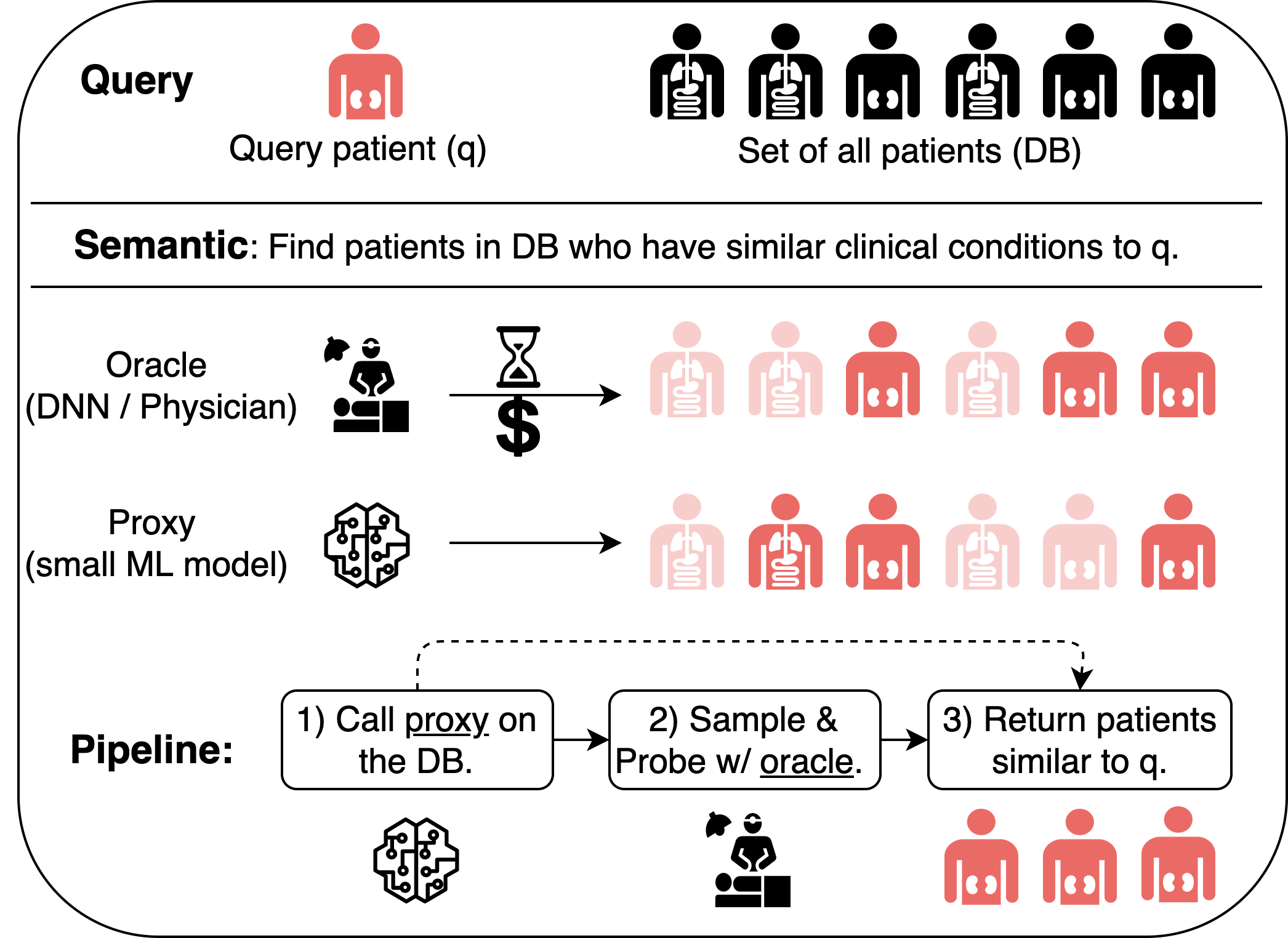
Figure 1. Query over ML predictions in medical domain.

The main focus of query processing over ML models has been to ensure efficiency without compromising accuracy (Zhou et al., 2020). One line of work, query inference, provides native relational support for ML operators using containerized solutions such as Amazon Aurora, or in-application solutions such as Google’s BigQuery ML and Microsoft’s Raven (Karanasos et al., 2020). Another line develops adaptive predictions for NNs by pruning examples based on their classification in early layers (Bolukbasi et al., 2017). Our aim is to enable queries in a way that is agnostic to the underlying prediction model. Hence, we develop an in-application approach where queries can be invoked on any ML prediction model.

Recent work  (Kang et al., 2017; Lu et al., 2018; Lai et al., 2021; Kang et al., 2020) proposes to use cheap proxy models that approximate ground truth oracle labels. Proxies are small neural models that either provide a confidence score (Kang et al., 2020; Yang et al., 2022; Lu et al., 2018) or distribution (Lai et al., 2021) for their predicted labels. Probabilistic predicates (PP) (Lu et al., 2018) and CORE (Yang et al., 2022) employ light-weight proxies to filter out unpromissing objects and empirically improve data reduction rates in query execution plans. Probabilistic Top-K (Lai et al., 2021) trains proxy models to generate oracle label distribution and delivers approximate Top-K solutions. Recently, in (Kang et al., 2020), the authors study queries with a minimum precision target (PT) or recall target (RT), and a fixed user-specified budget on the number of oracle calls. However, (i) setting an oracle budget is hard to get right. An underestimated budget may lead to trivial answers while overestimation causes unnecessary oracle usage, and (ii) setting only a minimum precision or only a minimum recall target, runs the risk of returning valid but uninformative answers: for RT, returning all objects in the DB is valid but has very poor precision; for PT, returning the empty set is valid but it has zero recall and is hence not useful in practice.

In this work, we consider oracle/proxy models with multi dimensional outputs. We propose a more useful problem of minimizing oracle usage for finding answers that meet a precision or recall target with provable statistical guarantees while achieving a maximal complementary rate (CR). The CR for an RT (resp. PT) query is precision (resp. recall). More formally, given a PT (resp. RT) query, we seek answers that (1) satisfy a target precision (resp. recall) with a probability higher than a desired threshold and (2) incur a minimal number of oracle calls, and (3) achieve the maximal CR subject to the oracle usage incurred in (2). We aim to minimize oracle usage since the oracle is significantly more expensive than the proxy.

Our problem raises three challenges: (1) identify high quality answers with statistical guarantees, (2) design strategies that exactly or approximately minimize oracle usage, and (3) achieve maximal CR subject to (2). We develop a class of strategies that are agnostic to the prediction model and are applicable both to RT and PT queries. The key idea of our approach is to approximate an oracle with a cheaper proxy model (Kang et al., 2017, 2020). In practice, the proxy could be a smaller and lower latency neural model. We consider a general pipeline for query answering which consists of three stages: (1) apply proxy on the DB, (2) sample & probe with oracle, (3) compute and return answers (see Figure 1). We instantiate our pipeline under two alternative assumptions. Under the Proxy Quality assumption, the proxy quality w.r.t. the oracle is quantified in a probabilistic manner which allows us to return high quality answers right after applying the proxy on the DB. We develop Algorithm PQA which efficiently finds high probability valid answers of maximal expected CR with zero oracle calls. We additionally design Algorithm PQE, a heuristic extension to PQA, to calibrate the correlation between the oracle and the proxy by incurring some oracle calls. If the proxy quality is hard to quantify, we have the Core Set Closure assumption under which we uniformly sample and probe a subset of objects to estimate valid answers to a given query. We introduce the notion of core set to find the optimal sample size and number of samples so as to ensure a minimal expected oracle usage to identify a valid answer with high probability. We use the proxy to improve answer CR heuristically. This leads to Algorithm CSC, which efficiently returns high probability valid answers with a minimal expected number of oracle calls, and an empirically good CR. We also design Algorithm CSE, a generalization of CSC, which calibrates core sets with extra oracle calls and ensures high success probability.

We conduct experiments on five real-world datasets and compare our algorithms to four baselines from recent work: (1) SUPG (Kang et al., 2020), (2) Top-K (Lai et al., 2021), a probabilistic Top-K approach that uses oracle score distribution to deliver approximate Top-K answers, (3) Sample2Test, a sample-based baseline adapted from the literature (Lu et al., 2018), and (4) Scan2Test, a simple baseline that returns answers by applying oracle on all objects, which is also compared with in  (Lai et al., 2021). Our experiments demonstrate that our algorithms find high quality answers with statistical guarantees even when baselines fail. More specifically, we analyze PQA and verify the optimality of its CR and success probability guarantee under the Proxy Quality assumption. We compare PQA with Top-K on a synthetic dataset and demonstrate that PQA returns high quality answers with zero oracle call while Top-K incurs a huge oracle cost. We analyze CSC to demonstrate its minimal oracle usage and success probability guarantee under the Core Set Closure assumption. We compare PQE, CSE, and baselines in terms of success probability and CR, under various oracle settings. We find that for RT queries, CSE has the best oracle efficiency and for PT queries, PQE is the most oracle efficient approach. Finally, we study scalability and find that CSE is the most efficient approach outperforming the strongest baseline by up to $87.5\%$.

In sum, we make the following contributions.

• We propose the problem of answering PT and RT queries with minimal oracle usage and maximal CR while meeting precision or recall targets with high probability (§ 2).

• We propose two assumptions (Proxy Quality and Core Set Closure), around which we develop four algorithms (PQA, PQE, CSC, and CSE) to solve the problem efficiently (§ 4).

• We run extensive experiments on five real-world datasets (§ 5) and show that: (i) our approaches yield valid answers with high probability; (ii) our approaches significantly outperform the state of the art w.r.t. CR and cost.

Complete details of proofs as well as additional experiments can be found in the full version (Ding et al., 2022).

2. Problem Studied

2.1. Use Cases

Example 0 (Image Retrieval).

The problem is to find images similar to a query image (Chen et al., 2021; Deniziak and Michno, 2016; Zheng et al., 2018). Metadata-based approaches use textual descriptions of images for quickly measuring similarity, but their quality heavily relies on image annotations (Deniziak and Michno, 2016). Current approaches for content-based image retrieval are built upon deep neural networks which provide high accuracy but are computationally expensive. Our goal is to support efficient high quality approximate image retrieval queries (Cao et al., 2016).

Example 0 (Preventive Medicine).

One of the greatest obstacles of preventive medicine is the limited time a physician has (Love, 1994; Brull et al., 1999; fra, [n.d.]; Rodrigues et al., 2020). Clinical Risk Prediction Models (CRPMs) are being developed to facilitate decision-making. CRPMs serve as prognosis prediction systems and predict the occurrence of specific diseases based on personalized medical records. Our goal is to extend queries to include CRPMs while offering statistical guarantees (Rodrigues-Jr et al., 2021; Choi et al., 2016; Li et al., 2020).

Example 0 (Video Analytics).

While DNNs have become effective for querying videos (Redmon et al., 2016), their inference cost becomes prohibitive as the model size increases. For example, to identify frames with a given class (e.g., ambulance) on a month-long traffic video, an advanced object detector such as YOLOv2 (Redmon and Farhadi, 2016) needs about 190 GPU hours and $380 for a cloud service (Hsieh et al., 2018). A specialized model can achieve high efficiency, e.g., up to $340\times$ faster than the full DNN, with sacrificed accuracy (Kang et al., 2017). Our goal is to efficiently generate high quality query answers by balancing the use of expensive high-accuracy models and cheap low-accuracy proxies (Hsieh et al., 2018; Kang et al., 2017, 2020).

2.2. Query

Our queries generalize Fixed-Radius Near Neighbor (FRNN) queries (Bentley, 1975). Given a dataset $D$, a query object $q$, a radius $r$, and a distance function $dist$, an FRNN query asks for all near neighbors of $q$ within radius $r$, i.e., $NN(q,r)=\{x\in D\mid dist(x,q)\leq r\}.$ In this paper, we are mainly interested in near neighbors of objects w.r.t. latent features, using a distance function defined on these features. In preventive medicine (fra, [n.d.]; Rodrigues et al., 2020), a latent feature may be the infection risk of a disease, which can be inferred from patient history, drug usage, and demographics. Latent features can be discovered by human experts (Lu et al., 2018) or powerful neural models, which we refer to as oracle, denoted $O$. The near neighbors of query object $q$ w.r.t. $O$ and radius $r$ are defined as $NN^{O}(q,r)=\{x\in D\mid dist(O(x),O(q))\leq r\}$. We will use the notation $NN^{O}$ when the query object $q$ and radius $r$ are clear from the context. An object $x\in D$ is an oracle neighbor of a query object w.r.t. radius $r$ if $x\in NN^{O}$. Retrieving the exact $NN^{O}$ requires calling the oracle on every single object in the DB, which is prohibitively expensive. Instead, we are interested in finding high quality answers with high probability (w.h.p.).

For any subset $S\subseteq D$, we denote by $N_{S}=|S\cap NN^{O}|$ the number of oracle neighbors in $S$. Define:

(1) $$\begin{split}M_{p}(S)&=N_{S}/|S|\hskip 14.22636ptM_{r}(S)=N_{S}/|NN^{O}|\end{split}$$

A query specifies a user-given measure $M$, which can be either $M_{p}$ for precision or $M_{r}$ for recall, to measure answer quality, and a target $\gamma\in(0,1)$. In the former case, it is called a Precision-Target (PT) query and in the latter, Recall-Target (RT) query. We call $Ans\subseteq D$ a valid answer iff $M(Ans)\geq\gamma$. For $M$, we use $\overline{M}$ to denote its complementary rate (CR): when $M=M_{p}$ (resp., $M_{r}$), $\overline{M}$ stands for $M_{r}$ (resp., $M_{p}$). Given a query, we are interested in returning valid answers w.h.p. For any $S\subseteq D$, the probability of success for $M(S)$ is $PoS(S,M,\gamma):=Pr[M(S)\geq\gamma]$. We generalize FRNN queries to Approximate Oracle-Sensitive FRNN (AOS-FRNN ) queries.

Definition 2.4 (AOS-FRNN Query).

Given a dataset $D$, a query object $q$, a radius $r$, a failure rate $\delta$, a main measure $M$ and corresponding target $\gamma\in(0,1)$, an AOS-FRNN query asks for a valid answer $Ans\subseteq D$ w.h.p., i.e., such that $PoS(Ans,M,\gamma)\geq 1-\delta$.

Effectively processing an AOS-FRNN query requires determining: (1) How many oracle calls are required to find a valid answer w.h.p.? and (2) How good is the returned answer under a given CR? The first question is important since oracle invocations are expensive and must be reduced. The second question is important because a technically valid answer could be uninformative. For instance, if a user specifies $M=M_{p}$ with a high target $\gamma$, the empty set is always a valid answer. Similarly, returning (nearly) the whole dataset is always a valid answer when $M=M_{r}$.

Problem 1 (AOS-FRNN Problem).

Given a dataset $D$ and an AOS-FRNN query $Q$, find a valid answer $Ans\subseteq D$ to $Q$ w.h.p. such that (i) the number of oracle calls incurred is minimal and (ii) the complementary rate $\overline{M}(Ans)$ achieved is maximal subject to (i).

The AOS-FRNN Problem is challenging given that we want to optimize two objectives (i.e., oracle usage and CR) under validity and success probability constraints. We will show that under certain conditions, we can efficiently return high probability valid answers with minimal or zero oracle calls and maximal expected CR.

3. Approach Overview

The key idea of our approach is to approximate an oracle with a cheaper proxy model  (Kang et al., 2017, 2020). In practice, compared to an expensive oracle $O$, a proxy $P$ could be a smaller and lower latency neural model. For brevity, when a query object $q$ is clear from the context, we use $dist^{P}(x)$ (resp. $dist^{O}(x)$) to denote $dist(P(x),O(q))$ (resp. $dist(O(x),O(q))$), for any $x\in D$.

Given a dataset $D$, define an index function $I:D\to\{i\mid 1\leq i\leq|D|\}$ that enumerates data objects in increasing order of their proxy distance, i.e., $\forall x_{i},x_{j}\in D$, $I(x_{i})\leq I(x_{j})$ if $dist^{P}(x_{i})\leq dist^{P}(x_{j})$. Denote by $D_{k}=\{x\in D\mid 1\leq I(x)\leq k\}$ the $k$ nearest neighbors of the query object w.r.t. the proxy distance. $D_{0}$ is the empty set. Given a query object $q$, for $x\in D$, we say that $k$ is the proxy index of $x$ if $k=I(x)$. In this case, we call $D_{k}$ the proxy prefix of $x$.

To solve the AOS-FRNN Problem with guarantees, we examine two alternative assumptions:

Assumption 1 (Proxy Quality): When the proxy quality w.r.t. the oracle can be quantified in a probabilistic manner, we aim to find high probability valid answers of maximal expected CRs with no oracle calls. We develop Algorithm PQA to do that. For $x\in D$, PQA assumes the conditional probability of $dist^{O}(x)$, given $dist^{P}(x)$. We can show that this assumption holds as long as data is i.i.d. (see §  4.1.1). This allows it to compute the success probability $PoS(S,M,\gamma)$ and expected CR $\mathbb{E}[\overline{M}(S)]$ for any answer $S\subseteq D$. We prove that the optimal answer to any given query is $D_{k^{*}}$ for some $0\leq k^{*}\leq|D|$. The optimal answer satisfies validity w.h.p. and has maximal expected CR. As $k^{*}$ is not known a priori, we explore the monotonicity of $PoS(D_{k},M,\gamma)$ and $\mathbb{E}[\overline{M}(D_{k})]$ w.r.t. $k$ in order to efficiently identify $D_{k^{*}}$. For RT queries, $PoS(D_{k},M,\gamma)$ monotonically increases as $k$ increases. We use binary search to identify the smallest $k=\underline{k}$ such that $PoS(D_{k},M,\gamma)\geq 1-\delta$. Next, we find $\underline{k}\leq k=k^{*}\leq|D|$ which maximizes $\mathbb{E}[\overline{M}(D_{k})]$ and return $D_{k^{*}}$ as the answer. For PT queries, $\mathbb{E}[\overline{M}(D_{k})]$ monotonically increases as $k$ increases. Thus, we incrementally compute $PoS(D_{k},M,\gamma)$ for $0\leq k\leq|D|$ and set $k^{*}$ as the largest $k$ s.t. $PoS(D_{k},M,\gamma)\geq 1-\delta$. We return $D_{k^{*}}$ as the answer. It is easy to see that $D_{k^{*}}$ is the optimal answer and no oracle call is invoked in computing it.

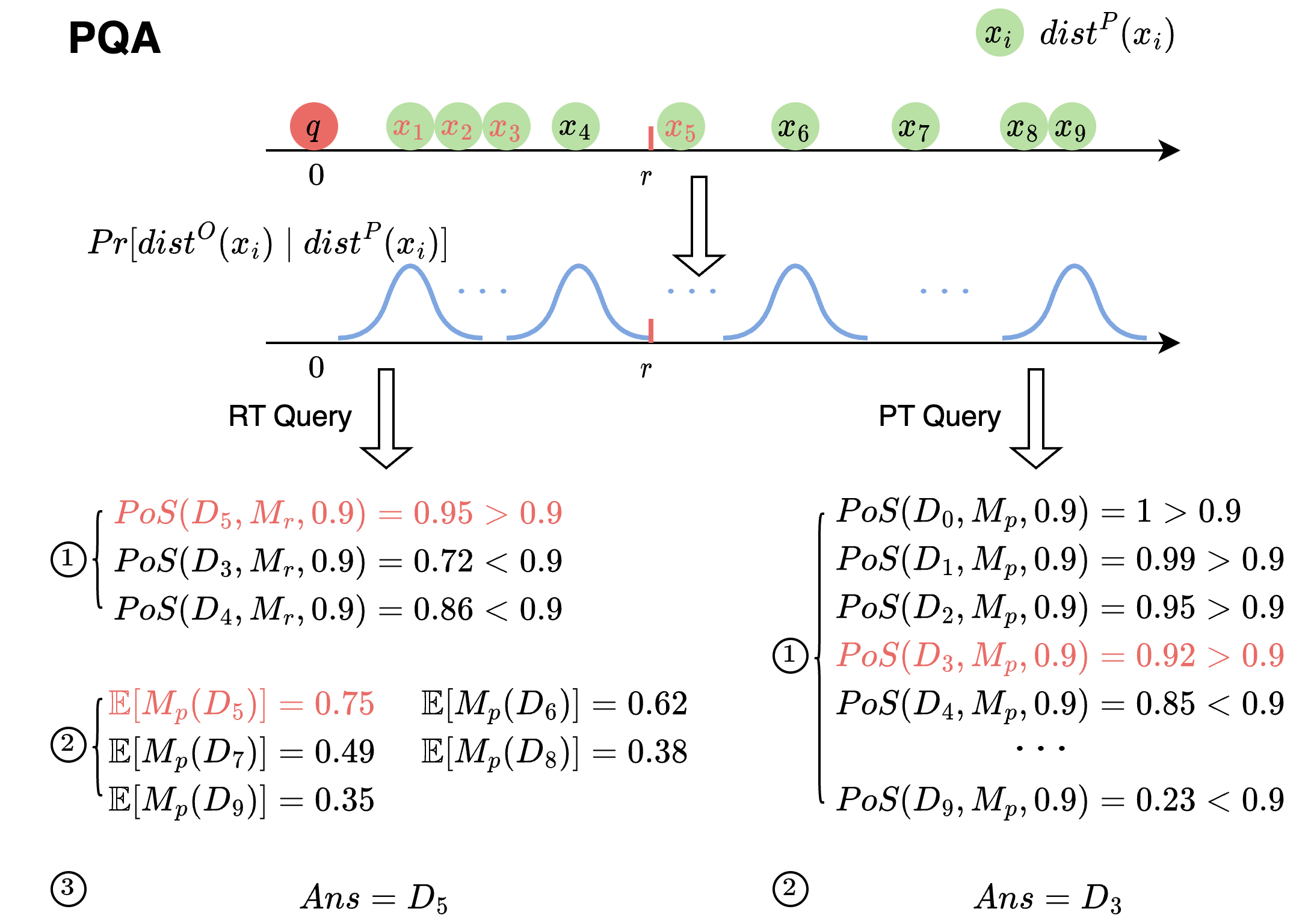
Figure 2. Example RT and PT query solved by PQA with $NN^{O}=\{x_{1},x_{2},x_{3},x_{5}\}$, $\gamma=0.9$, and $\delta=0.1$.

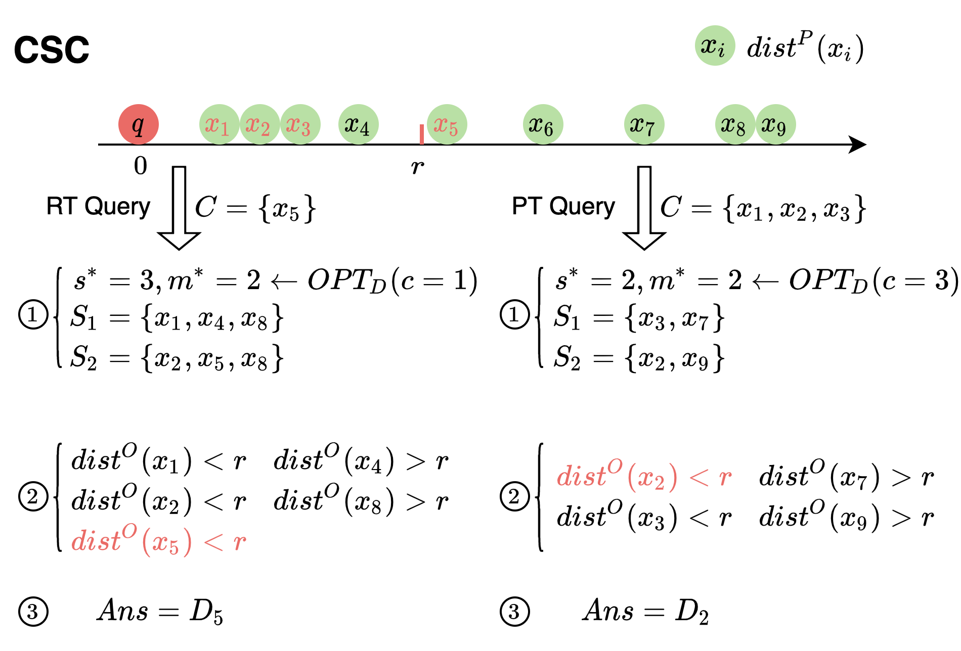
Figure 3. Example RT and PT query solved by CSC with $NN^{O}=\{x_{1},x_{2},x_{3},x_{5}\}$, $\gamma=0.9$, and $\delta=0.1$.

Example 0.

A (synthetic) illustrative example is shown in Figure 3. Consider a dataset $D=\{x_{1},x_{2},\cdots,x_{9}\}$. We show how to use PQA to solve the example RT and PT queries with $\gamma=0.9$, $\delta=0.1$ and a ground truth $NN^{O}=\{x_{1},x_{2},x_{3},x_{5}\}$. We first compute proxy distance $dist^{P}(x_{i})$ for each $x_{i}\in D$ and derive the oracle distance distribution $Pr[dist^{O}(x_{i})|dist^{P}(x_{i})]$ according to our assumption, which allows us to compute $PoS(S,M,\gamma)$ and $\mathbb{E}[\overline{M}(S)]$ for any $S\subseteq D$. We want to efficiently find the optimal answer $D_{k^{*}}$. In this example, $I(x_{i})=i$ and $D_{k}=\{x_{1},x_{2},\cdots,x_{k}\}$. For the RT query, we use binary search to find $\underline{k}=5$, i.e., the smallest $k$ satisfying $PoS(D_{k},M_{r},\gamma=0.9)\geq 1-\delta=0.9$. Next, we compute expected precision and return $D_{5}$ as the answer since $\mathbb{E}[M_{p}(D_{5})]=0.75\geq\mathbb{E}[M_{p}(D_{k})]$ for any $\underline{k}\leq k\leq|D|$. For the PT query, we compute $PoS(D_{k},M_{p},\gamma=0.9)$ for $0\leq k\leq|D|$ and return $D_{3}$ as the answer since $k=3$ is the largest $D_{k}$ satisfying $PoS(D_{k},M_{p},\gamma=0.9)\geq 1-\delta=0.9$.

Assumption 2 (Core Set Closure): When the proxy quality is hard to quantify, we aim to find $k^{*}$ s.t. $D_{k^{*}}$ is the optimal answer. Since computing $k^{*}$ exactly is expensive, we estimate it by sample and probe. Specifically, we uniformly draw $m$ samples of size $s$ each, from $D$ to estimate $k^{*}$ as $k_{\mathcal{S}}$ where $\mathcal{S}$ is the union of samples, and return $D_{k_{\mathcal{S}}}$ as the answer. For RT (resp. PT) queries, we set $k_{\mathcal{S}}$ as the largest (resp. smallest) $I(x)$, where $x$ is an oracle neighbor in $\mathcal{S}$. We seek the optimal values $s=s^{*}$ and $m=m^{*}$ which ensure $PoS(D_{k_{\mathcal{S}}},M,\gamma)\geq 1-\delta$ with a minimal expected number of oracle calls. For that, we introduce the notion of core set, denoted $C$. Given a query, the core set comprises all oracle neighbors $x\in NN^{O}$ whose proxy prefix $D_{I(x)}$ is a valid answer. We say the core set is closed w.r.t. a query $Q$ if one of the following holds: (i) $Q$ is a RT query and for every $x\in C$ any oracle neighbor whose proxy index is larger than that of $x$ is also in $C$; or (ii) $Q$ is a PT query and for every $x\in C$ any oracle neighbor whose proxy index is smaller than that of $x$ is also in $C$. Let $c$ denote the size of a given core set $C$. We show that if the core set $C$ is closed w.r.t. a query and $c$ is known, $s^{*}$ and $m^{*}$ can be found by solving an optimization problem with $c$ as the input (§ 4.2). We develop Algorithm CSC to efficiently solve this problem and return $D_{k_{\mathcal{S}}}$. CSC returns valid answers w.h.p. with a minimal expected oracle usage and empirically good CR.

Example 0.

The (synthetic) example in Figure 3 illustrates the idea behind Algorithm CSC. Consider the same setting as in Figure 3, where $D=\{x_{1},x_{2},\cdots,x_{9}\}$, and RT and PT queries with $\gamma=0.9$, $\delta=0.1$, ground truth $NN^{O}=\{x_{1},x_{2},x_{3},x_{5}\}$, and $D_{k}=\{x_{1},x_{2},\cdots,x_{k}\}$. For the RT query, $x_{5}$ is the only oracle neighbor whose proxy prefix is a valid answer. Therefore, $C=\{x_{5}\}$ and $C$ is closed. We can derive the optimal values $s^{*}=3$ and $m^{*}=2$, and uniformly draw samples $S_{1}$, $S_{2}$ from $D$. We then apply oracle on each $x_{i}\in\mathcal{S}=S_{1}\cup S_{2}$ and compute $dist^{O}(x_{i})$ accordingly. At the end, we set $k_{\mathcal{S}}=5$ and return $D_{5}$ as the answer since $x_{5}$ has the largest proxy index among sampled oracle neighbors $x_{1},x_{2},x_{5}$. For the PT query, the core set is $C=\{x_{1},x_{2},x_{3}\}$, which is closed. Similarly, we first derive the optimal values $s^{*}=2$ and $m^{*}=2$, and draw $S_{1}$, $S_{2}$ accordingly. Next, we apply the oracle on samples and compute the corresponding oracle distance. At the end, we set $k_{\mathcal{S}}=2$ and return $D_{2}$ as the answer since $x_{2}$ has the smallest proxy index among sampled oracle neighbors $x_{2},x_{3}$.

In case these assumptions do not hold, we develop PQE and CSE. PQE is a heuristic extension to PQA which calibrates oracle distance distribution by incurring some oracle calls. CSE complements CSC and ensures high success probability in general. The workflow and performance of all four approaches are summarized in Figure 4 and Table 1.

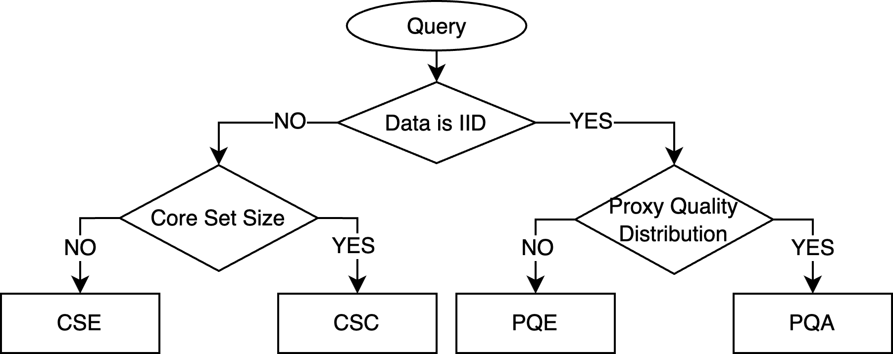
Figure 4. Workflow of different approaches.

	Success Prob.	Oracle Usage	CR	Assumption
PQA	$\mathbf{\geq 1-\delta}$	$\mathbf{0}$	MAX	Yes
CSC	$\mathbf{\geq 1-\delta}$	MIN	good	Yes
CSE	$\mathbf{\geq 1-\delta}$	small	good	No
PQE	high	small	good	No

Table 1. Performance of different approaches for queries with specified $\delta$. Provable guarantees are highlighted. Empirical performance is described by “high”, “small”, and “good”.

Table 2. Notation Summary

Symbol	Description	Symbol	Description
$dist^{O}(x)$	oracle distance	$r$	radius threshold
$dist^{P}(x)$	proxy distance	$C$, $c$	core set (size)
$NN^{O}$	oracle neighbors in DB	$\delta$	failure rate
$N_{S}$	# oracle neighbors in $S$	$I(x)$	proxy index of $x$
$M$, $\overline{M}$	main/comp. measure	$M_{p}$, $M_{r}$	precision/recall
$D_{k}$	$k$ proxy-nearest neighbors	$\gamma$	measure target
$k^{*}$	proxy index $I(x)$ of $x\in D$, s.t. $D_{I(x)}$ is the optimal answer.
$k_{\mathcal{S}}$	max (resp. min) $I(x)$ of $x\in\mathcal{S}\cap NN^{O}$ for RT (resp. PT) queries.

We will use $M$ and $\overline{M}$ when results hold for both PT and RT. We next describe our algorithms and provide a theoretical analysis.

4. Formal Analysis and Algorithms

4.1. Proxy Quality

In § 4.1.1, we formally state the Proxy Quality assumption and show how the success probability of a set $S\subseteq D$ can be computed. Then, we develop Algorithm PQA based on this assumption (§ 4.1.2) and analyze answer optimality (§ 4.1.3). In § 4.1.4, we develop Algorithm PQE to extend PQA to more general settings.

4.1.1. Proxy Quality Assumption

In many real-world applications, data is collected in i.i.d. manner (Lai et al., 2021; Lu et al., 2018). In our problem setting, the oracle and proxy are provided as input and serve as deterministic functions mapping a data object $x_{i}\in D$ to its prediction $O(x_{i})$ or $P(x_{i})$. The difference between oracle and proxy distances to a given query object can be seen as i.i.d. random variables, whose i.i.d. property comes from the underlying data collection process. Formally, the assumption states that given a query, the deviations between the proxy and oracle distances of different objects $x_{i}\in D$ are i.i.d. random variables: for $x_{i}\in D,\epsilon_{i}=dist^{O}(x_{i})-dist^{P}(x_{i})$, where $\epsilon_{i}$ are i.i.d., $\epsilon_{i}\sim\mathcal{X}$. In Figure 5 we report the distribution of $\epsilon_{i}$ on two real-world datasets, Mimic-III (Johnson et al., 2016) and night-street (Canel et al., 2019). It is clear that, with high frequency, $\epsilon_{i}$ takes on values close to $0$, which indicates that the proxy is of good quality and can properly approximate the oracle predictions.

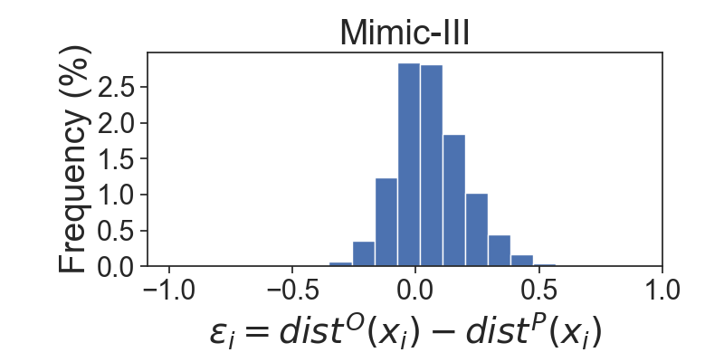
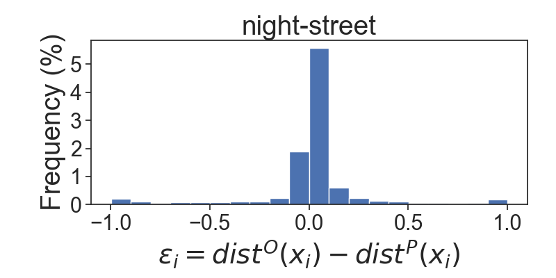
Figure 5. Distribution of $\epsilon_{i}=dist^{O}(x_{i})-dist^{P}(x_{i})$.

Under this assumption, we can compute the oracle distance distribution for any $x_{i}\in D$, after observing the proxy distance. The conditional probability of $x_{i}\in D$ being an oracle neighbor is:

(2) $$\begin{split}Pr[x_{i}\in NN^{O}\mid dist^{P}(x_{i})]&=Pr[dist^{O}(x_{i})\leq r\mid dist^{P}(x_{i})]\\ &=Pr[\epsilon_{i}\leq r-dist^{P}(x_{i})]\end{split}$$

The RHS of Eq. 2 is the cdf of $\epsilon_{i}\sim\mathcal{X}$ evaluated at $r-dist^{P}(x_{i})$, i.e., $CDF_{{\footnotesize\mathcal{X}}}(r-dist^{P}(x_{i}))$. For simplicity, define $\phi(x_{i}):=CDF_{\mathcal{X}}(r-dist^{P}(x_{i}))$ and $\Phi(D):=\{\phi(x_{i})\mid x_{i}\in D\}$. Notice, $\phi(x_{i})$ provides the probability that $x_{i}$ is an oracle neighbor. The overall success probability uses the possible world semantics (Moore, 1984). The success probability of a subset $S\subseteq D$ equals the sum of probabilities of all possible worlds in which $S$ has a high precision or recall w.r.t. the target $\gamma$. To compute the success probability of $S$, we seek the likelihood of any $S\subseteq D$ containing a certain number of oracle neighbors.

Recall that for any subset $S\subseteq D$, $N_{S}=|S\cap NN^{O}|$ is the number of oracle neighbors in $S$. $N_{S}$ is thus a random variable equal to the sum of $|S|$ independent Bernoulli trials, each of which has a success probability $\phi(x_{i})$, $x_{i}\in S$. Let $p_{N_{S}}(k):=Pr[N_{S}=k]$ be the probability mass function for any $S\subseteq D$ and $0\leq k\leq|S|$. We next discuss how to compute it efficiently.

An important fact is that, given $S\subseteq D$, $x_{i}\notin S$, $p_{N_{S\cup\{x_{i}\}}}$ and $p_{N_{S}}$ satisfy the following recurrence relation:

(3) $$\begin{split}p_{N_{S\cup\{x_{i}\}}}(k)=p_{N_{S}}(k-1)\cdot\phi(x_{i})+p_{N_{S}}(k)\cdot(1-\phi(x_{i}))\\ \end{split}$$

for $0\leq k\leq|S|+1$. Eq. 3 says how to compute the probability mass function $p_{N_{S\cup\{x_{i}\}}}$ from $p_{N_{S}}$, for any $S\subseteq D$ and $x_{i}\notin S$. This recurrence relation directly suggests a way to compute $p_{N_{S}}$ for any $S$ with incremental updates, called direct convolution (Biscarri et al., 2018). We start from $S=\varnothing$ and apply Eq. 3 recursively to compute $p_{N_{S}}$ for any $S\subseteq D$. $p_{N_{S}}$ is implemented by an array (we abbreviate $\phi(x_{i})$ as $\phi_{i}$). We initialize the array $p_{N_{S}}[0]=1$. We then iteratively update $p_{N_{S}}$ by including $x_{i}\in S$, $1\leq i\leq|S|$, in any order. The distribution updates are a direct implementation of Eq. 3.

We now discuss how to use $p_{N_{S}}$ to compute $PoS(S,M,\gamma)$, the success probability for $S$ to be a valid answer. We have the following fact, where $\overline{S}:=D\setminus S$:

Fact 1.

Given $S\subseteq D$ and $\gamma\in(0,1)$,

(4) $$\begin{split}PoS(S,M_{p},\gamma)&=Pr[\frac{N_{S}}{|S|}\geq\gamma]=\sum_{k=\lceil|S|\gamma\rceil}^{|S|}p_{N_{S}}(k)\\ \end{split}$$

(5) $$\begin{split}PoS(S,M_{r},\gamma)&=Pr[\frac{N_{S}}{|NN^{O}|}\geq\gamma]=\sum_{j=0}^{|S|}p_{N_{S}}(j)\sum_{k=0}^{\lfloor j(1-\gamma)/\gamma\rfloor}p_{N_{\overline{S}}}(k)\\ \end{split}$$

For PT queries, the precision of $S\subseteq D$ increases as $S$ contains more oracle neighbors. The probability of $S$ having a precision no less than $\gamma$ equals the probability of $S$ containing at least $|S|\gamma$ oracle neighbors, i.e., $Pr[N_{S}\geq|S|\gamma]$. Eq. 4 gives this probability.

For RT queries, the recall of $S\subseteq D$ increases as $S$ contains more oracle neighbors relative to the complement $\overline{S}=D\setminus S$: if $S$ contains $0\leq j\leq|S|$ oracle neighbors, the conditional probability of $S$ having a recall no less than $\gamma$ equals the probability that $\overline{S}$ contains no more than $j(1-\gamma)/\gamma$ oracle neighbors, i.e., $Pr[N_{\overline{S}}\leq j(1-\gamma)/\gamma]$. By the law of total probability (Grimmett, 1986), the overall success probability $PoS(S,M_{r},\gamma)$ equals the summation of the product between the conditional success probability, $Pr[N_{\overline{S}}\leq j(1-\gamma)/\gamma]$, and the marginal probability, $Pr[N_{S}=j]$, $0\leq j\leq|S|$. Using Eq. 5, we use $p_{N_{S}}$ and $p_{N_{\overline{S}}}$ to compute this probability.

Fact 1 gives a direct way to compute $PoS(S,M,\gamma)$ for any $S\subseteq D$ for a given query. We also leverage Eq. 4 and Eq. 5 iteratively.

4.1.2. Algorithm PQA

We develop PQA (Algorithm 1) which returns high probability valid answers with zero oracle calls and maximal expected CR, under the Proxy Quality assumption. For PT queries, PQA-PT computes the largest $k$ s.t. $PoS(D_{k},M_{p},\gamma)\geq 1-\delta$, $0\leq k\leq|D|$, denoted $k^{*}$. Notice that $PoS(S,M_{p},\gamma)$ can be derived from $p_{N_{S}}$ in linear time, and $p_{N_{S}}$ can be computed from $p_{N_{S\setminus\{x_{i}\}}}$ in linear time, for any $x_{i}\in S\subseteq D$. PQA-PT incrementally computes $p_{N_{D_{k}}}$ for each $0\leq k\leq|D|$ and $PoS(D_{k},M_{p},\gamma)$ accordingly. At the end, PQA-PT returns $D_{k^{*}}$ where $k^{*}=\max\{0\leq k\leq|D|\mid PoS(D_{k},M_{p},\gamma)\geq 1-\delta\}$. For RT queries, PQA-RT uses binary search to identify the smallest $k=\underline{k}$ such that $PoS(D_{k},M,\gamma)\geq 1-\delta$. Next, PQA-RT computes the expected CR of $D_{k}$ for each $\underline{k}\leq k\leq|D|$, and returns $D_{k^{*}}$ where $k^{*}=\operatorname*{argmax}_{\underline{k}\leq k\leq|D|}\mathbb{E}[M_{p}(D_{k})]$.

The algorithm is presented in Algorithm 1. PQA-PT is given in lines 1-1. In lines 1-1, we incrementally compute $p_{N_{D_{k}}}$ for $0\leq k\leq|D|$. In lines 1-1, we keep tracking the largest $k=k^{*}$, $0\leq k\leq|D|$, such that $PoS(D_{k},M_{p},\gamma)\geq 1-\delta$, and return $D_{k^{*}}$ as the answer. The overall time complexity is $O(|D|^{2})$. PQA-RT is given in lines 1-1. In lines 1-1, we use binary search to find the smallest $k=\underline{k}$ such that $PoS(D_{k},M_{r},\gamma)\geq 1-\delta$. Next, in lines 1-1, we compute $\mathbb{E}[M_{p}(D_{k})]$ for each $\underline{k}\leq k\leq|D|$ and return $D_{k^{*}}$ with the maximal expected CR. Binary search invokes $O(log(|D|))$ times $p_{N_{S}}$ computation, each of which is of $O(|D|^{2})$. The overall time complexity is therefore $O(log(|D|)|D|^{2})$.

1

2

3

4Function PQA-PT($\Phi_{D}=\Phi(D)$, $\gamma$, $\delta$) :

5      $p_{N_{S}}[0]\leftarrow 1$; $k^{*}\leftarrow 0$

6       for $i\leftarrow 1,2,\cdots,|D|$ do

             $p_{N_{S}}\leftarrow$ IncrementalUpdate($p_{N_{S}}$, $\Phi_{D}[i]$, $i$)

              /* Eq.3 */

             if PoS-Mp($p_{N_{S}}$, $\gamma$) $\geq 1-\delta$

              /* Eq.4 */

7              then

8                  $k^{*}\leftarrow i$

9            

10      return $D_{k^{*}}$

11

12Function PQA-RT($\Phi_{D}=\Phi(D)$, $\gamma$, $\delta$) :

13       $\underline{k}\leftarrow 1$; $\overline{k}\leftarrow|D|$

14       while $\underline{k}<\overline{k}$ do

15             $mid\leftarrow\lfloor(\underline{k}+\overline{k})/2\rfloor$

             $p_{N_{S}}\leftarrow$ pNs($\Phi(S)$); $p_{N_{\overline{S}}}\leftarrow$ pNs($\Phi(\overline{S})$)

              /* Eq.3 */

             if PoS-Mr($p_{N_{S}}$, $p_{N_{\overline{S}}}$, $\gamma$) $<1-\delta$

              /* Eq.5 */

16             then

17                  $\underline{k}\leftarrow mid+1$

18            else

19                  $\overline{k}\leftarrow mid$

20            

21       $p_{N_{S}}\leftarrow$ pNs($\Phi(D_{\underline{k}})$)

       $E\overline{M}\leftarrow$ Sum($\{p_{N_{S}}[i]\cdot i/{\underline{k}}\mid 1\leq i\leq\underline{k}\}$)

        /* $\mathbb{E}[M_{p}(S)]$ */

22       for $i\leftarrow\underline{k}+1,\underline{k}+2,\cdots,|D|$ do

             $p_{N_{S}}\leftarrow$ IncrementalUpdate($p_{N_{S}}$, $\Phi_{D}[i]$, $i$)

              /* Eq.3 */

23             $E\overline{M}^{\prime}\leftarrow$ Sum($\{p_{N_{S}}[j]\cdot j/{i}\mid 1\leq j\leq i\}$)

24             if $E\overline{M}^{\prime}>E\overline{M}$ then

25                   $E\overline{M}\leftarrow E\overline{M}^{\prime}$; $k^{*}\leftarrow i$

26            

27      return $D_{k^{*}}$

Algorithm 1 PQA

4.1.3. PQA Optimality

We first show that there exists some $D_{k^{*}}$, s.t. it is an optimal answer. We then explore the monotonicity relation between $D_{k}$ and $D_{k+1}$ w.r.t. success probability and expected CR, to efficiently find $D_{k^{*}}$. Finally, we show that answers returned by PQA are optimal for any query (proofs in the full version (Ding et al., 2022)).

For $S\subseteq D$, we are interested in two operations to generate new answers: (i) replace $x_{i}\in S$ with $x_{j}\notin S$, and (ii) append $S$ with a new object $x\notin S$. We first show that for any $S\subseteq D$, both success probability $PoS(S,M,\gamma)$ and expected CR $\mathbb{E}(\overline{M}(S))$ are monotone under the replacement operation.

Lemma 0 (Monotonicity of Replacement).

Let $S\subseteq D$, $x_{i}\in S$, and $x_{j}\notin S$. Denote $S^{\prime}=S\cup\{x_{j}\}\setminus\{x_{i}\}$. For all $\gamma\in(0,1)$, if $\phi(x_{i})\leq\phi(x_{j})$, then

(6) $$\begin{split}PoS(S,M,\gamma)&\leq PoS(S^{\prime},M,\gamma)\hskip 14.22636pt\mbox{and}\hskip 14.22636pt\mathbb{E}[\overline{M}(S)]\leq\mathbb{E}[\overline{M}(S^{\prime})]\\ \end{split}$$

Proof Sketch.

The proof leverages the notion of usual stochastic order (Nair et al., 2013). ∎

Lemma 4.1 says that, given $S\subseteq D$, if we replace $x_{i}\in S$ with $x_{j}\notin S$, where $x_{j}$ is more likely to be an oracle neighbor, both the success probability and the expected CR of $S$ will monotonically increase, for a given query. Lemma 4.1 can be used to prune out a majority of unpromising solutions in the early stage of query processing. Specifically, given a query, we show that for any $0\leq k\leq|D|$, $D_{k}$ is optimal among all answers of size $k$. Recall $D_{k}$ is the set of $k$ nearest neighbors of the query object w.r.t. the proxy distance. Formally,

Theorem 4.2.

For all $\gamma\in(0,1)$, $\forall 0\leq k\leq|D|$, $D_{k}$ has the highest success probability and expected CR among all $S\subseteq D$ with $|S|=k$.

Theorem 4.2 entails that, given a query, there exists some $0\leq k^{*}\leq|D|$ such that $D_{k^{*}}$ is guaranteed to be an optimal answer. We study the append operation and have the following result.

Lemma 0 (Monotonicity of Append).

For all $\gamma\in(0,1)$ and $0\leq k\leq|D|-1$,

(7) $$\begin{split}PoS(D_{k},M_{r},\gamma)&\leq PoS(D_{k+1},M_{r},\gamma)\hskip 5.69046pt\mathbb{E}[M_{r}(D_{k})]\leq\mathbb{E}[M_{r}(D_{k+1})]\end{split}$$

Lemma 4.3 states that increasing $k$ leads to an increase both in the probability for $D_{k}$ to have a high recall and its expected recall. In other words, the success probability of $D_{k}$ monotonically increases for RT queries, and the expected CR of $D_{k}$ monotonically increases for PT queries, as $k$ increases.

By Theorem 4.2 and Lemma 4.3, for any given query, the answer $D_{k^{*}}$ returned by Algorithm PQA clearly has high success probability and the maximal expected CR, implying it is an optimal answer.

4.1.4. Algorithm PQE

Recall that Algorithm PQA requires $\Phi(D)$ as an input. In a general setting, when $\Phi(D)$ is unknown or Proxy Quality Assumption does not hold, we heuristically fit a normal distribution by sampling and probing on a limited number of objects, where the limit is controlled by a budget parameter. The resulting algorithm is PQE (Algorithm 2).

That is, in PQE, we employ $\epsilon_{i}\sim\mathcal{N}(\mu,\sigma)$ for all $x_{i}\in D$. Specifically, we choose $\mu=0$, which amounts to assuming that the proxy is an unbiased estimator of the oracle. For $\sigma$, given a budget $b$, we sample and probe $b$ objects to estimate $\sigma$, denoted $\hat{\sigma}$. We further introduce a hyper-parameter $\sigma_{0}$ to represent the deviation from the Proxy Quality assumption. In the ideal case where Proxy Quality holds, $\sigma_{0}=0$. We heuristically choose $\sigma=\hat{\sigma}+\sigma_{0}$. We use $\mathcal{N}(\mu,\sigma)$ to compute $\Phi(D)$ and pass it to PQA to find the answers.

1

2

3Function PQE($D$, $\gamma$, $\delta$, $r$, $b$, $\sigma_{0}$):

4       $S\leftarrow$ Sample($D$, $b$)

5       $\sigma\leftarrow\sigma_{0}+$ std($\{dist^{O}(x)-dist^{P}(x)\mid x\in S\}$)

6       $\Phi_{D}\leftarrow\{$ CDF_N(0,σ)($r-dist^{P}(x)$) $\mid x\in D\}$

7       if RT query  then

8            return PQA-RT($\Phi_{D}$, $\gamma$, $\delta$)

9      else

10            return PQA-PT($\Phi_{D}$, $\gamma$, $\delta$)

11      

Algorithm 2 PQE

Algorithm 2 details the steps. In lines 2-2, we draw a sample $S\subseteq D$ of $|S|=b$ objects to estimate $\sigma$ and compute $\Phi(D)$. In lines 2-2, we invoke Algorithm PQA with $\Phi(D)$ for PT or RT queries. The overall time complexity is dominated by Algorithm PQA: the additional time complexity on top of PQA is $O(|D|)$.

We now introduce Core Set Closure assumption, our second alternative assumption, and develop two algorithms $CSC$ and $CSE$.

4.2. Core Set Closure

In § 4.2.1, we formally introduce the Core Set Closure assumption and show how to find the optimal sample and probe strategy when core set size is known. We also analyze the case when core set size is unknown and show how to ensure high success probability. In § 4.2.2, we develop Algorithms CSC and CSE based on this. In § 4.2.3, we discuss how to support progressive query processing.

4.2.1. Core Set Closure Assumption

For a query, we define the core set as the set of all oracle neighbors whose proxy prefix is a valid answer. We use $c$ to denote the size of a given core set $C$. A core set $C$ is closed w.r.t. an RT (resp. PT) query if for any $x\in C$, any oracle neighbor whose proxy index is larger (resp. smaller) than that of $x$ is also an element of $C$. Core Set Closure assumption says that, for any given query, the core set is closed w.r.t. that query.

For RT queries, the core set is always closed, because as the proxy index of oracle neighbors increases, the recall of corresponding proxy prefix monotonically increases. For PT queries, with a properly tuned proxy, the core set is likely to be closed in practice. In Figure 6, we report the average $Precision(D_{k})$ over $100$ random queries on two real datasets, Mimic-III (Johnson et al., 2016) and night-street (Canel et al., 2019). It is clear that the precision of proxy prefix $D_{k}$ monotonically decrease as $k$ increases on both datasets, which shows the core set closure property for PT queries.

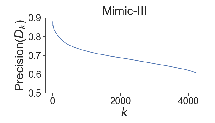
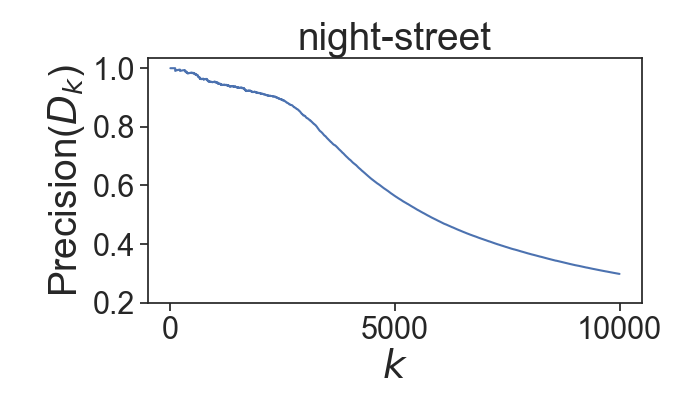
Figure 6. Precision of proxy prefixes $D_{k}$.

We uniformly draw $m$ samples of size $s$ from $D$ to derive $k_{\mathcal{S}}$ where $\mathcal{S}$ is the union of samples, and return $D_{k_{\mathcal{S}}}$ as the answer. Recall that $k_{\mathcal{S}}$ is the largest (resp. smallest) $I(x)$ for RT (resp. PT) queries, where $x$ is determined to be an oracle neighbor by probing $\mathcal{S}$ (see § 3, Assumption 2). If the core set $C$ is closed w.r.t. a given query, the success probability of $D_{k_{\mathcal{S}}}$ is the likelihood of $\mathcal{S}$ intersecting with $C$, i.e., $PoS(D_{k_{\mathcal{S}}},M,\gamma)=Pr[\mathcal{S}\cap C\neq\varnothing]$. Since samples are drawn uniformly, we have $Pr[\mathcal{S}\cap C\neq\varnothing]=1-(\binom{|D|-c}{s}/\binom{|D|}{s})^{m}=1-(\prod_{i=0}^{c-1}\frac{|D|-s-i}{|D|-i})^{m}$, where $s$ is the sample size and $m$ is the number of samples. We denote $f(|D|,s,m,c):=1-(\prod_{i=0}^{c-1}\frac{|D|-s-i}{|D|-i})^{m}$.

When $\mathbf{c}$ is known

Given $s$ and $m$, the expected number of oracle calls made by the sample and probe strategy is $EOC(s,m)=\mathbb{E}[|\mathcal{S}|]=|D|(1-(1-\frac{s}{|D|})^{m})$. When $c$ is known, we can determine $s=s^{*}$ and $m=m^{*}$, which minimizes $EOC(s,m)$ while ensuring $f(|D|,s,m,c)\geq 1-\delta$, by solving the following equation:

(8) $$\begin{split}\min_{s,m}\quad&EOC(s,m)=|D|(1-(1-\frac{s}{|D|})^{m})\\ \textrm{s.t.}\quad&f(|D|,s,m,c)\geq 1-\delta\\ \end{split}$$

By plugging in the expression for $f(|D|,s,m,c)$, the constraint can be simplified to $m\geq\lceil\frac{log(\delta)}{log(\prod_{i=0}^{c-1}\frac{|D|-s-i}{|D|-i})}\rceil$. By denoting the RHS as $\underline{m}(s)$, we can rewrite the constraint as $m\geq\underline{m}(s)$ for simplicity. Note, for a given $s$, $EOC(s,m)$ monotonically increases as $m$ increases. For a fixed $s$, the optimal $m$ which ensures a high success probability (i.e., $\geq 1-\delta$) and minimizes $EOC(s,m)$ is clearly, $m=\underline{m}(s)$. As a special case, we have $m^{*}=\underline{m}(s^{*})$. Thus, a naive approach for finding $s^{*}$ and $m^{*}$ is to compute $EOC(s,m)$ for each $1\leq s\leq|D|$ and $m=\underline{m}(s)$ and picking the best.

Such exhaustive search for the exact value of $s^{*}$ and $m^{*}$, however, can be expensive in a large DB. Instead, we are interested in approximation solutions with good guarantees, which we develop next. Given a query, let $(s,m)$ denote the sample size and number of samples used by a strategy. Then $|D|-EOC(s,m)$ denotes the expected number of saved oracle calls compared with the exhaustive approach of probing every object in the DB. Define the savings ratio as $\xi(s,m)=\frac{|D|-EOC(s,m)}{|D|-EOC(s^{*},m^{*})}$. It denotes the fraction of oracle calls saved by strategy $(s,m)$ compared to the optimal strategy $(s^{*},m^{*})$. A larger $\xi$ indicates a better approximation, and the optimal strategy $(s^{*},m^{*})$ yields $\xi(s^{*},m^{*})=1$.

Let us examine the special cases where either $s=1$ or $m=1$. For $s=1$, we let $m=\underline{m}(1)$, and

(9) $$\xi_{s=1}:=\xi(1,\underline{m}(1))\geq\delta^{\frac{-1}{c}(\frac{1}{|D|}-\frac{|D|}{|D|-1)}}\cdot(1-1/|D|)$$

For $m=1$, we set $s=s_{1}:=\lceil\frac{-log(\delta)}{\sum_{i=0}^{c-1}\frac{1}{|D|-i}}\rceil$ to ensure high success probability, and

(10) $$\xi_{m=1}:=\xi(s_{1},1)\geq\delta^{\frac{-1}{|D|c}}\cdot(1-1/|D|+log(\delta)/c)$$

In practice where e.g., $\delta=0.1$, $|D|=10,000$, and $c=100$, we have both $\xi_{s=1}$ and $\xi_{m=1}$ being no less than $97.7\%$, that is, if we fix either $s=1$ or $m=1$ as above, the saved oracle usage is at least $97.7\%$ of what the optimal strategy $(s^{*},m^{*})$ achieves. Thus, either of them can be used as an approximation to the optimal strategy.

When $c$ is unknown

We incur extra oracle calls and apply Hoeffding Bounds (Vershynin, 2018) to ensure high success probability.

Proposition 4.4 (Hoeffding Bounds).

Let $\{X_{i}\}_{i=1}^{n}$ be independent random variables, with $X_{i}\in\{0,1\}$ and let $\mathbb{E}[X_{i}]=\mu$. Let $\hat{\mu}=\frac{1}{n}\sum_{i=1}^{n}X_{i}$. Then for $\forall\epsilon\geq 0$, we have the concentration bound

(11) $$Pr[\hat{\mu}-\epsilon\leq\mu]\geq 1-exp(-2n\epsilon^{2})$$

For an RT query with target $\gamma$, we can derive a probabilistic lower bound for $c$ as follows. For an RT query, the core set $C$ consists of the top $(1-\gamma)\times 100$ % oracle neighbors of largest proxy indices. That is, we can write $c=\lfloor|NN^{O}|(1-\gamma)\rfloor+1$. When $s$ and $m$ are fixed, $f(|D|,s,m,c)$ monotonically increases as $c$ increases. Given $\delta_{r}\in(0,1)$, let $\underline{c}$ denote a probabilistic lower bound of $c$, i.e., $Pr[c\geq\underline{c}]\geq 1-\delta_{r}$. We can solve Eq. 8, either exactly or approximately as needed, subject to a more stringent constraint $f(|D|,s,m,\underline{c})\geq\frac{1-\delta}{1-\delta_{r}}$ to find $s$ and $m$, which ensures an overall success probability no less than $1-\delta$. We show how to derive such probabilistic lower bound $\underline{c}$ using Hoeffding Bounds.

Randomly draw $x_{i}\in D$. Define $X_{i}=1$ iff $dist^{O}(x_{i})\leq r$. We have $\mu_{D}:=\mathbb{E}[X_{i}]=\frac{|NN^{O}|}{|D|}$. Randomly draw $\{x_{i}\}_{i=1}^{n}$ with replacement. Denote $\hat{\mu_{D}}=\frac{1}{n}\sum_{i=1}^{n}X_{i}$. For any $\epsilon_{r},\delta_{r}\in(0,1)$, by Hoeffding Bounds, we have $Pr[\hat{\mu_{D}}-\epsilon_{r}\leq\mu_{D}]\geq 1-\delta_{r}$ if $n\geq\frac{log(\delta_{r})}{-2\epsilon_{r}^{2}}$. For an RT query with target $\gamma$, since $c=\lfloor|NN^{O}|(1-\gamma)\rfloor+1$, and we have $Pr[c\geq\lfloor|D|(\hat{\mu_{D}}-\epsilon_{r})(1-\gamma)\rfloor+1]\geq 1-\delta_{r}$, if $n\geq\frac{log(\delta_{r})}{-2\epsilon_{r}^{2}}$. We denote the probabilistic lower bound $\underline{c}:=\lfloor|D|(\hat{\mu_{D}}-\epsilon_{r})(1-\gamma)\rfloor+1$.

For PT queries, such $\underline{c}$ is hard to obtain. Given $\delta$ and $k$, we apply Hoeffding Bounds in a similar way to derive a probabilistic lower bound for the precision $M_{p}(D_{k})$, denoted as $\underline{\mu_{D_{k}}}$. That is, $Pr[M_{p}(D_{k})\geq\underline{\mu_{D_{k}}}]\geq 1-\delta$. For a PT query with target $\gamma$, $D_{k}$ is a high probability valid answer if $\underline{\mu_{D_{k}}}\geq\gamma$. We use heuristics to identify $D_{k}$ of high $\underline{\mu_{D_{k}}}$ and good CR (details in § 4.2.2).

4.2.2. Algorithms with Core Set Closure

Algorithm CSC

Algorithm CSC returns high probability valid answers with a minimal expected number of oracle calls and empirically good CR, under Core Set Closure and taking $c$ as input. CSC is presented in Algorithm 3. We compute $s^{*}$ and $m^{*}$ in line 3 either exactly or approximately, and draw samples in line 3. In lines 3 to 3, we compute $k_{\mathcal{S}}$ according to the query type and return $D_{k_{\mathcal{S}}}$ as the answer. The exact solution to Eq.8 requires $O(c|D|)$ operations while approximate solutions take $O(c)$ operations. The time complexity is dominated by accessing proxy prefixes, which requires sorting all objects w.r.t. proxy distance taking $O(|D|log(|D|))$.

1

2

3Function CSC($D$, $c$, $\delta$):

       $s^{*},m^{*}\leftarrow$ getsm($|D|$, $c$, $\delta$)

        /* Solve Eq.8 */

4       $\mathcal{S}\leftarrow$ UniformSample($D$, $s^{*}$, $m^{*}$)

5       if RT query  then

6            $k_{\mathcal{S}}\leftarrow\max\{I(x)\mid x\in\mathcal{S}\land dist^{O}(x)\leq r\}$

7      else

8            $k_{\mathcal{S}}\leftarrow\min\{I(x)\mid x\in\mathcal{S}\land dist^{O}(x)\leq r\}$

9      return $D_{k_{\mathcal{S}}}$

Algorithm 3 CSC

Algorithm CSE

Algorithm CSE incurs more oracle calls and returns high probability valid answers in general settings where $c$ is unknown or Core Set Closure assumption does not hold.

CSE is presented in Algorithm 4. CSE-RT is given in lines 4 to 4. Given $\epsilon_{r}$ and $\delta_{r}$, we sample and probe $n=\lceil\frac{log(\delta_{r})}{-2\epsilon_{r}^{2}}\rceil$ objects to derive $\underline{c}$. Then, we invoke Algorithm CSC to process the query subject to $f(|D|,s,m,\underline{c})\geq\frac{1-\delta}{1-\delta_{r}}$. CSE-PT is given in lines 4 to 4. We use CSC to find good answer candidates, and apply Hoeffding Bounds to return high probability valid answers. Specifically, given a query and budget $b^{\prime}$, we sample and probe $b^{\prime}$ objects to estimate $c$, then invoke CSC with the estimation to compute $D_{k_{1}}$ (lines 4 to 4). We also use the same sample to estimate the largest $k=k_{2}$ such that $D_{k}$ has a sampled precision no less than $\gamma$ (line 4). To improve CR (i.e., recall for PT queries), we set $\hat{k}=\max\{k_{1},k_{2}\}$ and consider $D_{\hat{k}}$ as the answer candidate (line 4). In lines 4 to 4, given $\epsilon_{p}$, we draw samples and estimate a probabilistic lower bound for $M_{p}(D_{\hat{k}})$ by applying Hoeffding Bounds. For a PT query with target $\gamma$, we return $D_{\hat{k}}$ if the probabilistic lower bound is no less than $\gamma$. O/w, we return all oracle neighbors identified from samples. The overall time complexity is dominated by CSC and is also $O(|D|log(|D|))$.

4.2.3. Progressive Query Processing

We observe that though we minimize the oracle usage, for some challenging queries the bare minimum of oracle calls can still be too high. We propose progressive query processing for that. Recall that, our CSC and CSE approaches draw $m$ samples of size $s$ to compute $k_{\mathcal{S}}$ and return $D_{k_{\mathcal{S}}}$ as the answer. Instead of computing $k_{\mathcal{S}}$ after seeing all the samples, we can derive $k_{\mathcal{S}}^{\prime}$ after seeing each sample and use $k_{\mathcal{S}}^{\prime}$ to select answers with adaptive success probability bounds that are progressively better and better. We can keep refining $k_{\mathcal{S}}^{\prime}$ when we see more samples, eventually approaching $k_{\mathcal{S}}$, but the user can terminate the evaluation at any time based on the oracle cost incurred thus far.

1

2Function CSE-RT($D$, $\delta$) :

3       $\hat{\mu_{D}}\leftarrow$ HoeffdingEst($D$, $\delta_{r}$, $\epsilon_{r}$)

4       $\underline{c}\leftarrow\lfloor|D|(\hat{\mu_{D}}-\epsilon_{r})(1-\gamma)\rfloor+1$

5      

6      return CSC($D$, $\underline{c}$, $\frac{1-\delta}{1-\delta_{r}}$)

7

8Function CSE-PT($D$, $\delta$):

9       $S\leftarrow$ UniformSample($D$, $b^{\prime}$)

10       $\hat{c}\leftarrow\frac{|D|}{|S|}\cdot\text{the size of core set w.r.t. }S$

11       $D_{k_{1}}\leftarrow$ CSC($D$, $\hat{c}$, $1-\delta$)

12       $k_{2}\leftarrow\max\{I(x)\mid x\in S\land M_{p}(D_{I(x)}\cap S)\geq\gamma\}$

13       $\hat{k}\leftarrow\max\{k_{1},k_{2}\}$

14       $\underline{\mu_{D_{\hat{k}}}}\leftarrow$ HoeffdingEst($D_{\hat{k}}$, $\delta$, $\epsilon_{p}$) $-\epsilon_{p}$

15      if $\underline{\mu_{D_{\hat{k}}}}\geq\gamma$ then

16            return $D_{\hat{k}}$

17      else

18            return $\{x\in S\mid dist^{O}(x)\leq r\}$

19      

20

21Function HoeffdingEst($D$, $\delta$, $\epsilon$):

22       $S\leftarrow$ UniformSample($D$, $\lceil\frac{log(\delta)}{-2\epsilon^{2}}\rceil$)

23       return $\hat{\mu}\leftarrow\frac{|\{x\in S\mid dist^{O}(x)\leq r\}|}{|S|}$

24      

25

Algorithm 4 CSE

5. Experiments

Our extensive experiments (1) assess the performance of PQA to demonstrate its optimality w.r.t. CR and success probability under Proxy Quality assumption (§ 5.2), (2) assess the performance of CSC to demonstrate its minimal oracle usage and success probability under Core Set Closure assumption (§ 5.3), (3) compare PQE, CSE with the baselines on CR and success probability under the same oracle usage (§ 5.4) and under varied oracle budgets (§ 5.5). (4) Compare PQE, CSE with the baselines w.r.t. query time (§ 5.6). (5) Compare PQE, CSE with the baselines w.r.t. CPU overhead, CR, and success probability on datasets of various sizes and domains (§ 5.7).

5.1. Experimental Setup

5.1.1. Datasets and Proxy Models

Multi-label Image Recognition

VOC (Everingham et al., 2010) and COCO (Lin et al., 2014) are widely used benchmarks in multi-label recognition tasks. The validation set of COCO consists of $40,504$ images from $80$ classes, and VOC contains $4,952$ images from $20$ object categories. We also uniformly sample a $8000$-image subset from COCO, denoted as COCO (small). We use COCO and COCO (small) in different experiments.

Medical

Mimic-III (Johnson et al., 2016) and eICU (Pollard et al., 2018) are two publicly available clinical datasets, that include patient trajectories, demographics collected by daily ICU admissions, and clinical measurements. After pruning records with only one admission, we obtain a Mimic-III subset of $4,243$ records and an eICU subset of $8,235$ records.

Video

We use the night-street dataset (Canel et al., 2019) to support queries over classification tasks. Each video frame has a Boolean label indicating whether or not it contains a car. We uniformly draw a subset of $10,000$ frames from the original dataset for evaluation.

Datasets	Oracle	Proxy	Query targets
VOC&COCO	Human labeler	ML-GCN(Chen et al., 2019)	Similar images
Mimic-III&eICU	Physicians	LIG-Doctor(Rodrigues-Jr et al., 2021)	Similar patients
night-street	Mask R-CNN(He et al., 2017)	ResNet-50(He et al., 2015)	Car frames

5.1.2. Baselines

We consider the following baselines.

SUPG The closest work to ours is SUPG (Kang et al., 2020). SUPG uses oracle $O^{\prime}$ with a Boolean output and a proxy model $P^{\prime}$ which outputs a score in $[0,1]$. Given a query object $q$ and a radius $r$, our problem can be mapped to a binary classification problem: for each object $x$, is it a near neighbor to $q$ w.r.t. $r$? Given oracle $O$ and proxy $P$ for our problem, a natural oracle predicate for SUPG should output $1$ when the given object is a near neighbor and $0$ otherwise. This translates to $O^{\prime}(x)=1$ iff $dist^{O}(x)<=r$. Similarly, a natural proxy model for SUPG should give high scores when the corresponding object is more probable to be a near neighbor. As illustrated in Figure 5, with a properly chosen proxy, proxy distance $dist^{P}(.)$ is a good approximation for oracle distance $dist^{O}(.)$. Given that $dist^{P}(x)\in[0,1]$ in our problem, we choose $P^{\prime}(x)=1-dist^{P}(x)$ as the proxy model for SUPG. Intuitively, if object $x$ has a small proxy distance, $x$ is more likely to have a small oracle distance as well and hence more probable to be classified as $O^{\prime}(x)=1$, which is properly reflected by a high value of $P^{\prime}(x)$.

Probabilistic Top-K (Lai et al., 2021). This baseline studies approximate Top-K queries and delivers solutions with statistical guarantees. Given a query, there exists a direct mapping from our FRNN query to a Top-K query. For example, given a query object $q$ and radius $r$, an FRNN query asks for an answer $Ans$ which comprises all near-neighbours within the radius $r$ to $q$. Naturally, we can re-write this query in Top-K semantics: given query object $q$, return the Top-$K$ nearest neighbors to $q$ where $K=|Ans|$ according to the aforementioned FRNN query. Furthermore, this Top-K baseline relies on distribution over oracle predictions, which can be obtained from our Proxy Quality assumption in PQA.

Sample2Test Given an FRNN RT (resp. PT) query, this baseline first probes samples w.r.t. a given oracle budget, and then selects the optimal proxy prefix as the answer according to sample precision (resp. recall). This is the approach used in probabilistic predicates (PP) (Lu et al., 2018), NoScope (Kang et al., 2017), and also serves as a baseline in SUPG (Kang et al., 2020). Given a sample $S\subset D$ and a proxy index $k$, denote $S^{k}=S\cap D_{k}$. The sample precision at $k$ is $Precision_{S}(k)=\frac{|S^{k}\cap NN^{O}|}{|S^{k}|}$ and the sample recall is $Recall_{S}(k)=\frac{|S^{k}\cap NN^{O}|}{|S\cap NN^{O}|}$. Given dataset $D$ and the target $\gamma$, this baseline returns $D_{k^{\prime}}$ where $k^{\prime}=max\{1\leq k\leq|D|\mid Precision_{S}(k)\geq\gamma\}$ for PT queries, and $k^{\prime}=min\{1\leq k\leq|D|\mid Recall_{S}(k)\geq\gamma\}$ for RT queries. We select the largest (resp. smallest) proxy prefix for PT (resp. RT) to improve CR.

Scan2Test We also consider the naive approach which probes all objects with the oracle and selects the correct answer set for a given query. This approach is used as the baseline in (Lai et al., 2021).

5.1.3. Evaluation Measures

For both RT and PT queries, we are interested in three measures: (i) empirical success probability in relation to the required success probabilities; (ii) average CR of answers returned by different methods; and (iii) query processing time including (a) CPU overhead and (b) number of oracle calls. We do not compare proxy time since it is identical for all approaches and is only a fraction of the overall query processing time.

5.1.4. Protocol

Our evaluation protocol randomly chooses several query objects from a dataset and aggregates our measures for those query objects. In Section 5.2, we randomly choose $200$ query objects and aggregate their results. In other experiments, we randomly choose $50$ query objects and execute each query $10$ times and aggregate their results. This is because PQA is deterministic while other algorithms are subject to randomness, so we average over multiple trials. We use cosine distance whenever the model outputs are multi-dimensional vectors: $dist_{cos}(\mathbf{y_{1}},\mathbf{y_{2}})=1-\frac{\mathbf{y_{1}\cdot y_{2}}}{\|\mathbf{y_{1}}\|\cdot\|\mathbf{y_{2}}\|}$, given its wide application in proximity query processing (Alodadi and Janeja, 2015; Mingdong et al., 2018; Lahitani et al., 2016). When the output is scalar (e.g., Boolean labels), we use the absolute difference $dist_{abs}(\mathbf{y_{1}},\mathbf{y_{2}})=|\mathbf{y_{1}}-\mathbf{y_{2}}|$ as the distance function, which allows us to generalize SUPG query with boolean oracle predicates. In all cases, the radius threshold is $r=0.9$. The choice of distances and thresholds has no impact on our statistical guarantees.

Default values. Unless otherwise stated, we set $\gamma$ (recall and precision targets) to $0.95$ and $\delta$ to $0.1$ in all our experiments. We add a black dashed line ($-\cdot-$) at the level of $1-\delta$ in figures to help visually track the success probability of each approach. We empirically choose $\sigma_{0}=0.3$ for PQE, $\epsilon_{p}=0.1\%$ and $b^{\prime}=100$ for CSE-PT, $\epsilon_{r}=10\%$ and $\delta_{r}=0.05$ for CSE-RT according to our experiment results. We choose a small $\epsilon_{p}$ for CSE-PT to improve the probabilistic lower bound for precision, and a relatively large $\epsilon_{r}$ for CSE-RT to reduce the oracle usage incurred by applying Hoeffding Bounds. In addition, we only report results of CSE when $m=1$ (see Eq. 10) given its dominating performance over other $m$ settings.

Our algorithms are implemented in Python 3.7 and experiments are conducted on a M1 Pro chip @ $3.22$GHz with a 16GB RAM.

5.2. PQA Success at Maximal CR

PQA finds high probability valid answers of maximal expected CR with zero oracle calls, whenever Proxy Quality assumption holds (§ 4.1). We test it on two semi-synthetic datasets. Specifically, we use real proxy distances from VOC and eICU, and synthesize oracle distances with a normal distribution $\mathcal{N}(0,\sigma=0.1)$. We clip the normal distribution to $[0,1]$ to agree with the output range of our distance measures. We demonstrate CR maximality and success probability guarantees of PQA by comparing it with a series of variants. Recall that PQA returns the top-$k^{*}$ objects of smallest proxy distances as the answer. We measure the success probability and CR when using a perturbed $k^{*}$. We try perturbations ranging from $-20\%$ to $20\%$ by returning top-$(1+perturb)\cdot k^{*}$ for $-20\%\leq perturb\leq 20\%$.

The results are shown in Figure 9. The two top plots summarize RT queries. Recall $\delta=0.1$, which requires success probability being no less than $90\%$. On VOC, with zero perturbation, PQA achieves a $92\%$ empirical success probability and $39\%$ CR for RT queries. On eICU, the empirical success probability and CR are $90\%$ and $38\%$ respectively. With negative perturbation, empirical success probability quickly shrinks to nearly zero; with positive perturbation, CR starts to drop. This observation clearly demonstrates that PQA gives the highest answer CR while respecting the success probability constraint. The two bottom plots are for PT queries, and are similar to RT. The unperturbed PQA achieves $94\%$ empirical success probability on both datasets, a $53\%$ CR on VOC, and a $42\%$ CR on eICU. Any perturbation to $k^{*}$ either fails the success probability constraint or degrades CR.

We compare PQA and Top-K on the same semi-synthetic VOC dataset (see Figure 9). Both approaches achieve desired success probability targets. However, Top-K suffers from huge oracle usage while PQA needs no oracle calls, indicating PQA is capable of efficient query processing when proxy quality distribution is known. Furthermore, we investigate the sensitivity of PQA to $\sigma$, shown in Figure 9. We test $PQA$ on VOC with various $\sigma$ values and report PQE performance for comparison purposes. As $\sigma$ increases, for both query types, the success probability of PQA increases while CR decreases. This agrees with the intuition that, as the proxy quality gets worse, PQA becomes more conservative to improve success probability at the cost of CR degradation. Since PQE does not rely on external $\sigma$, both success probability and CR are constant and higher than PQA, given that PQE has the flexibility to probe samples with the oracle.

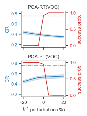
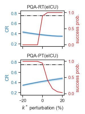
Figure 7. PQA with perturbed $k^{*}$ on VOC and eICU datasets.

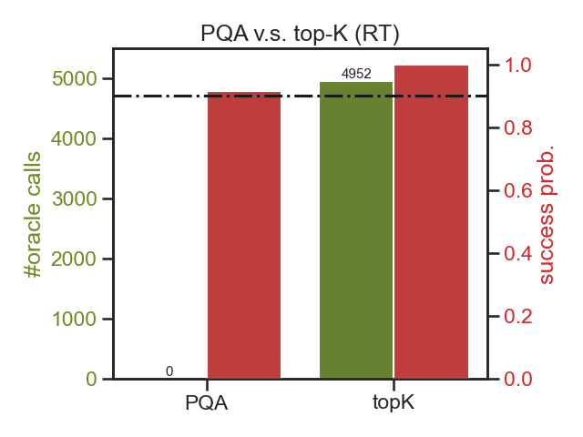
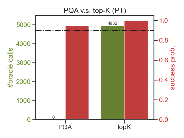
Figure 8. Comparison of PQA and Top-K on VOC.

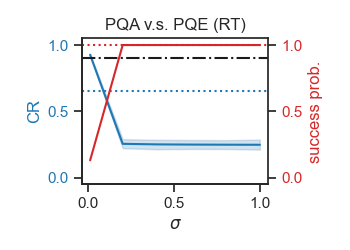
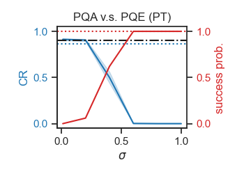
Figure 9. PQA (solid line) v.s. PQE (dotted line) on VOC.

5.3. CSC with Minimal Oracle Usage

CSC ensures high success probabilities with minimal oracle usage under Core Set Closure assumption (§ 4.2). We implement an exact algorithm and two approximation algorithms to compute $s^{*}$ and $m^{*}$ (§ 4.2.1), Approx-s1 and Approx-m1. We compare these algorithms to two baselines, Rand-s and Rand-sm. Specifically, Rand-s randomly chooses $s$ and sets $m=\underline{m}(s)$, whereas Rand-sm chooses both $s,m$ at random. For each query, we precompute the core set size and feed it to all approaches. We study the empirical success probability and oracle usage on VOC and eICU. The results for RT and PT queries are reported in Figure 10. Especially, we report standard deviation of oracle usage for both query types on both datasets. We also report CPU overheads in Figure 12.

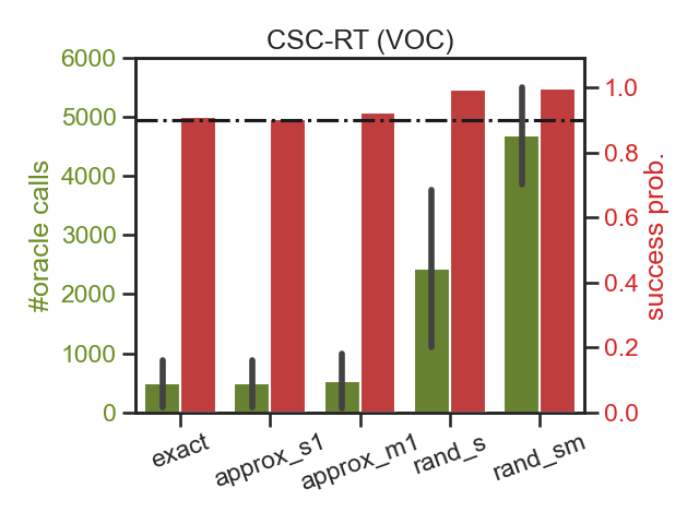
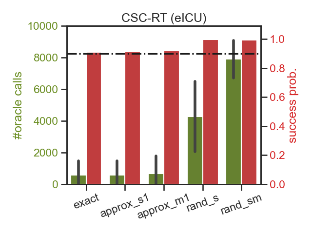
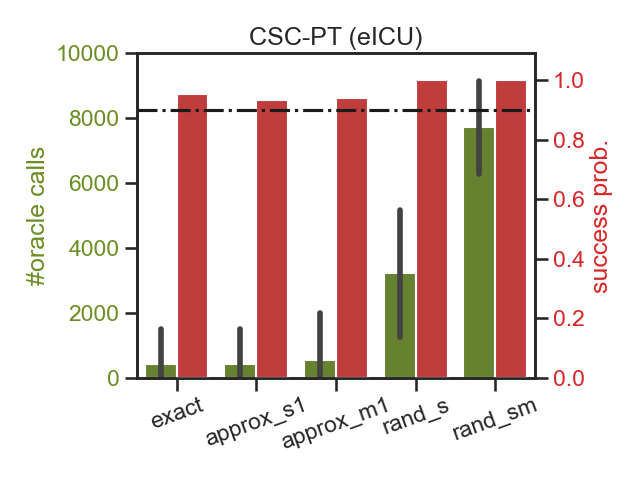
Figure 10. Oracle usage and empirical success probability by CSC-RT and CSC-PT.

For RT queries, all approaches achieve high empirical success probability. The exact algorithm invokes the oracle on only $9.8\%$ objects in VOC and $7.1\%$ objects in eICU. The oracle usage of approximation algorithms is just up to $1.1\%$ more than the exact algorithm. However, the baseline Rand-s applies the oracle on at least $49.3\%$ objects and Rand-sm makes oracles calls on at least $94.6\%$ objects.

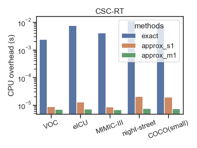
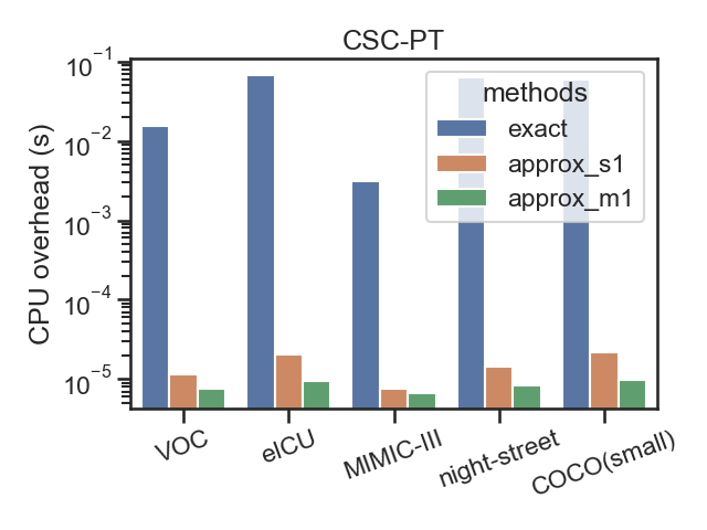
Figure 11. CSC CPU overheads

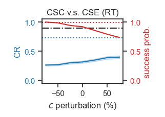
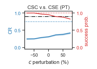
Figure 12. CSC (solid line) v.s. CSE (dotted line) on VOC.

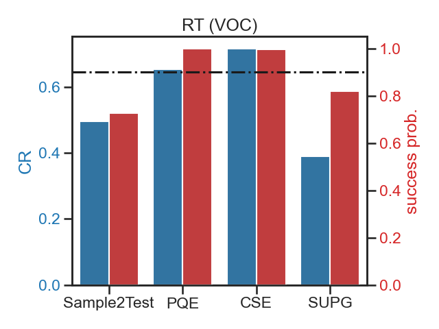
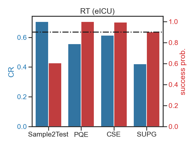
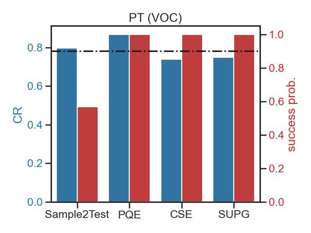
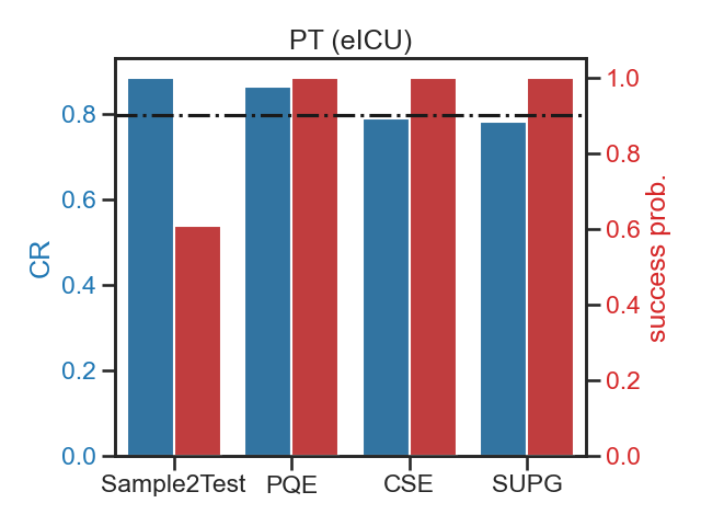
Figure 13. CR and empirical success probability by PQE, CSE, SUPG, Sample2Test.

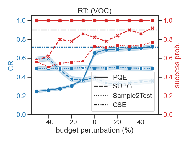
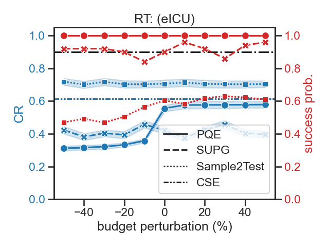
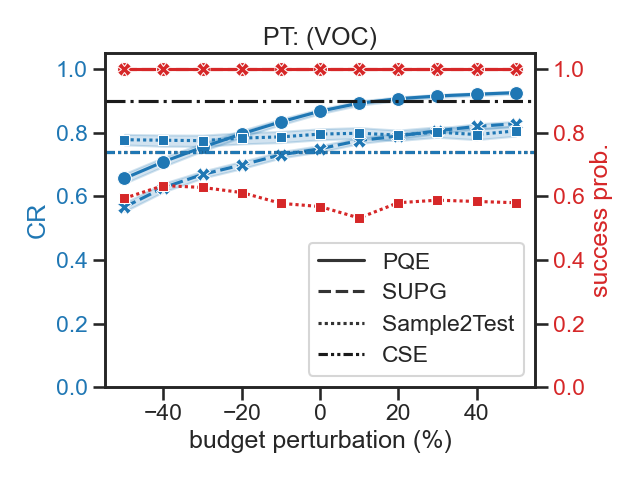
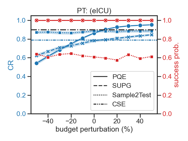
Figure 14. CR and empirical success probability by PQE, SUPG, Sample2Test with perturbed budget from CSE

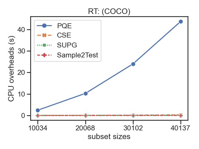
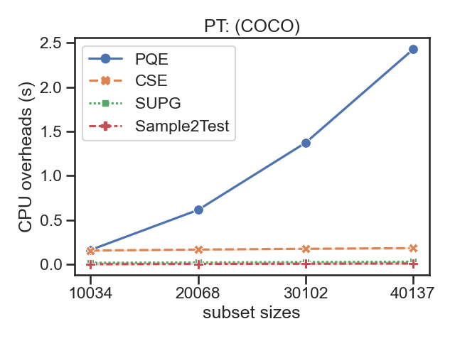
Figure 15. Scalability test: CPU overheads

Results of PT queries are similar to RT. All approaches achieve high empirical success probability. The exact algorithm has the smallest oracle usage, which accounts for $8.1\%$ objects in VOC and $5.2\%$ objects in eICU. The approximation algorithms incur an oracle usage which is just up to $2.1\%$ higher than the exact algorithm. The baseline method Rand-s calls the oracle on at least $39\%$ objects, and Rand-sm makes oracle calls for at least $93.7\%$ objects.

We are also interested in the CPU overhead of the exact algorithm and the two approximation algorithms. Results on our five real-world datasets are summarized in Figure 12. Clearly, the exact algorithm has a larger CPU overhead in comparison to the two approximation algorithms. Specifically, the approximation algorithms achieve a speedup up to $1466\times$ for RT queries and $7391\times$ for PT queries on CPU overheads, in comparison to the exact method.

On VOC, we investigate how sensitive CSC is to the input core set size $c$ and include CSE performance for the same query for comparison (Figure 12). As $c$ increases, for both query types, success probability of CSC decreases and CR increases. Since CSE estimates $c$ internally, both success probability and CR are agnostic to external $c$ changes. Note that the CSE performance is generally better than CSC, which is attributed to the fact that CSE has more flexibility to probe objects with oracle for the additional $c$ estimation.

5.4. CSE and PQE vs SUPG and Sample2Test

We implement CSE and PQE and compare them to SUPG and Sample2Test. For a fair comparison, we use the oracle usage incurred by CSE as the budget for PQE, SUPG, and Sample2Test. We measure empirical success probability and CR on VOC and eICU (Figure 14). For RT, CSE and PQE achieve high empirical success probability on both datasets, while SUPG fails the success threshold empirically by a margin of $10\%$ on VOC. On CR, PQE outperforms SUPG by a margin up to $26\%$, and CSE outperforms SUPG up to $33\%$. For PT, all approaches achieve high empirical success probability. On CR, PQE outperforms SUPG by up to $12\%$ and CSE achieves comparable CR to SUPG. Sample2Test continuously fails the success probability for both query types on both datasets.

Failures of SUPG on RT queries stem from the sample mean and variance it uses without error bounds, which introduces uncontrolled uncertainty and degrades statistical guarantees.

5.5. Oracle Efficiency

To measure Oracle efficiency, we perturb the oracle usage incurred by CSE and use it as the budget for PQE, SUPG, Sample2Test. The CR of CSE is also plotted as a baseline. Results are in Figure 14. For RT queries, PQE achieves high empirical success probability on both datasets, while SUPG and Sample2Test fails frequently on VOC especially with small budgets. This indicates that CSE is the most oracle efficient approach for RT queries. For PT queries, all approaches except Sample2Test achieve high empirical success probability on both datasets.

5.6. Time Efficiency

The running time of a query is composed of CPU overhead and model usage including proxy and oracle calls. We measure CPU overhead for each approach locally and approximate model usage by timing the number of model calls and average time taken by each call. For instance, on medical datasets (MIMIC-III & eICU), the oracle is a human physician whose average diagnosis time is $15$ minutes (Tai-Seale et al., 2007), while the proxy is a recurrent neural network taking roughly $1$ millisecond for each call (Rodrigues-Jr et al., 2021). Results are reported in Table 6, 6 with the best results in bold and saving ratios w.r.t. SUPG. For both query types, Sample2Test and Scan2Test are the two most time-consuming approaches.

Time / Hours	PQE	CSE	SUPG	Scan2Test	Sample2Test
VOC	21.22	15.88	24.12	27.51	26.84
COCO(small)	32.21	19.66	30.46	44.44	44.06
MIMIC-III	124.3	108.1	865	1061	1045.08
eICU	1337.3	679.2	925	2059	2009.16
night-street	0.38	0.11	0.19	1.11	1.15

Table 3. RT queries: query time by CSE, PQE, and baselines

Time / Hours	PQE	CSE	SUPG	Scan2Test	Sample2Test
VOC	4.71	6.3	7.52	27.51	26.41
COCO(small)	11.93	13.18	19.45	44.44	39.97
MIMIC-III	997.3	132.7	158.4	1061	1060.69
eICU	569.4	617.3	871.1	2059	1973.64
night-street	0.28	0.25	0.35	1.11	1.17

Table 4. PT queries: query time by CSE, PQE, and baselines.

—D—	Success Prob.	CR
	PQE/CSE/SUPG/Sample2Test	PQE/CSE/SUPG/Sample2Test
10034	1/0.99/0.78/0.69	0.72/0.74/0.46/0.53
20068	1/0.99/0.76/0.59	0.65/0.66/0.46/0.58
30102	1/0.99/0.76/0.65	0.63/0.65/0.44/0.5
40137	1/0.98/0.75/0.66	0.68/0.69/0.5/0.54

Table 5. Scalability test for RT queries

—D—	Success Prob.	CR
	PQE/CSE/SUPG/Sample2Test	PQE/CSE/SUPG/Sample2Test
10034	1/1/1/0.52	0.73/0.67/0.59/0.73
20068	1/1/1/0.48	0.69/0.65/0.59/0.71
30102	1/1/1/0.5	0.66/0.64/0.62/0.68
40137	1/1/1/0.51	0.67/0.64/0.66/0.74

Table 6. Scalability test for PT queries

5.7. Scalability

We measure CPU overhead, success probability, and CR of PQE, CSE, SUPG, and Sample2Test. We uniformly draw subsets of the original COCO dataset ($25\%$, $50\%$, $75\%$, and $100\%$). To make a fair comparison, we use the oracle usage incurred by CSE as the budget for PQE and SUPG. Results are reported in Figure 15 and Table 6, 6. For RT queries, CSE, SUPG, and Sample2Test have a reasonably low CPU overhead. For PT queries, PQE has the highest CPU overhead, $2.5$ seconds per query, while the overhead of CSE, SUPG, and Sample2Test is less than $0.2$ seconds.

6. Related Work

Query approximation. Query approximation techniques (Li and Li, 2018) can be categorized into (1) online aggregation: select samples online and use them to answer OLAP queries, and (2) offline synopses generation to facilitate OLAP queries. Our work adopts a probabilistic top-k approach (Theobald et al., 2004) and is significantly different from these.

FRNN query. FRNN query answering systems (Bentley, 1975; Bentley et al., 1977) build spatial indexes on the whole DB, which requires oracle calls on every single object. Our work focuses on reducing the oracle usage and is clearly distinguished from this line of work.

Optimizing ML inference. Several recent approaches were proposed to speed up the application of an ML model. Existing approaches follow either an in-database (Crankshaw et al., 2017) or in-application approach (Ahmed et al., 2019). Amazon Aurora is an example of an in-database containerized solution that enables external calls from SQL queries to ML models in SageMaker. Containerized execution introduces overhead in prediction latency. To mitigate that, Google’s BigQuery ML and Microsoft’s Raven were developed (Karanasos et al., 2020). Compared to Raven, BigQuery ML relies mostly on hard-coded models and targets batch predictions, since it inherits a relatively high startup cost. Raven and its runtime environment ONNX (Chen et al., 2018) offer the additional ability to make tuple-level inference.

Combining queries and ML inference. Bolukbasi et al. (Bolukbasi et al., 2017) enable incremental predictions for neural networks. Computation time is reduced by pruning examples that are classified in earlier layers, selected adaptively. Kang et al. (Kang et al., 2017) present NOSCOPE, a system for querying videos that can reduce the cost of neural network video analysis by up to three orders of magnitude via inference-optimized model search. Lu et al. (Lu et al., 2018) and Yang et al. (Yang et al., 2022) use probabilistic predicates to filter data blobs that do not satisfy the query and empirically increase data reduction rates. Anderson et al. (Anderson et al., 2019) use a hierarchical model to reduce the runtime cost of queries over visual content. Gao et al. (Gao et al., 2021) introduce a Multi-Level Splitting Sampling to let one ”promising” sample path prefix generate multiple ”offspring” paths, and direct Monte-Carlo based simulations toward more promising paths. Lai et al. (Lai et al., 2021) studies approximate Top-K query with light-weight proxy models that generate oracle label distribution. Recent work that proposed to use cheap proxy models, such as image classifiers, to identify an approximate set of data points satisfying a query (Kang et al., 2020), is by far the closest to our work, albeit they require a budget.

7. Conclusion and Discussion

We formalize and solve precision-target and recall-target queries, two paradigms that are well-suited for querying the results of ML predictions. We propose two assumptions and develop four algorithms. Our extensive experiments on five real-world datasets show that our approach enjoys statistical guarantees with a small cost and a good complementary rate, i.e., a good balance between recall and precision rates.

Our framework can be extended to optimize a query workload using metric properties like triangle inequality (Augustine et al., 2021). Consider the objects $\{q_{1},q_{2},x\}$. Suppose that we first choose $q_{1}$ as the query object, and compute the proxy distances $dist^{P}(q_{1},q_{2})$ and $dist^{P}(q_{1},x)$ to find answers using our approaches. Next, when we choose $q_{2}$ as the query object, by leveraging triangle inequality, we can lower bound $dist^{P}(q_{2},x)$ as $dist^{P}(q_{2},x)\geq|dist^{P}(q_{1},q_{2})-dist^{P}(q_{1},x)|$. If this bound is high, we can safely avoid applying the probe to $x$ for query $q_{2}$. We can extend our framework to multiple proxies at different accuracy and cost levels. This represents real-world scenarios where proxies are derived from huge neural models by activating specific subnetworks (Bolukbasi et al., 2017). It is clear that, with multiple proxy models, the search space for our optimization problem will exponentially increase. Secondly, by introducing proxies with various cost and accuracy levels, optimizing efficiency would go beyond simply counting oracle calls, and would yield a linear programming problem. We are currently exploring possible solutions.

Appendix A Appendix

A.1. Proof of Lemma 4.1

In order to prove Lemma 4.1, we need to introduce the notion of the usual stochastic order (Nair et al., 2013) , $\leq_{st}$.

Definition A.1 (Usual Stochastic Order).

Let $X$ and $Y$ be two random variables such that $Pr[X\geq x]\leq Pr[Y\geq x],\,\forall x\in(-\infty,\infty)$. Then $X$ is said to be smaller than $Y$ in the usual stochastic order (denoted by $X\leq_{st}Y$).

One important property for usual stochastic order is as follows,

Proposition A.2.

Let $X$ and $Y$ be two random variables. If $X\leq_{st}Y$, then $\mathbb{E}[\psi(X)]\leq\mathbb{E}[\psi(Y)]$ for all increasing function $\psi$ for which the expectations exist.

The proof of Proposition A.2 relies on constructing upper sets on the domain of $X$ and $Y$, which is beyond the scope of this paper. We refer interested readers to the literature (Nair et al., 2013) for more details.

Now, we can prove Lemma 4.1.

Proof.

Given $\gamma$, we first show $PoS(S,M,\gamma)\leq PoS(S^{\prime},M,\gamma)$ and then $\mathbb{E}[\overline{M}(S)]\leq\mathbb{E}[\overline{M}(S^{\prime})]$.

Recall $PoS(S,M,\gamma)=Pr[M(S)\geq\gamma]$. A sufficient condition for $PoS(S,M,\gamma)\leq PoS(S^{\prime},M,\gamma)$ is $M_{p}(S)\leq_{st}M_{p}(S^{\prime})$ and $M_{r}(S)\leq_{st}M_{r}(S^{\prime})$. We first discuss $M=M_{p}$, and then $M=M_{r}$. We abbreviate $\phi(x_{i})$, $\phi(x_{j})$ as $\phi_{i}$, $\phi_{j}$ for brevity.

When $M=M_{p}$, define random variables $X=N_{S\setminus\{x_{i}\}}$, $Y=N_{S}$, and $Z=N_{S^{\prime}}$. By equation 4, we have $Pr[M_{p}(S)\geq\gamma]=Pr[Y\geq\lceil|S|\gamma\rceil]$. The following relation holds,

(12) $$\begin{split}Pr[Y\geq\lceil|S|\gamma\rceil]&=Pr[X\geq\lceil|S|\gamma\rceil](1-\phi_{i})+Pr[X\geq\lceil|S|\gamma\rceil-1]\phi_{i}\\ &=\phi_{i}\cdot Pr[X=\lceil|S|\gamma\rceil-1]+Pr[X\geq\lceil|S|\gamma\rceil]\end{split}$$

where the last step is due to $Pr[X\geq\lceil|S|\gamma\rceil-1]-Pr[X\geq\lceil|S|\gamma\rceil]=Pr[X=\lceil|S|\gamma\rceil-1]$. Similarly, we have

(13) $$Pr[Z\geq\lceil|S|\gamma\rceil]=\phi_{j}\cdot Pr[X=\lceil|S|\gamma\rceil-1]+Pr[X\geq\lceil|S|\gamma\rceil]$$

Since $\phi_{i}\leq\phi_{j}$, we have $Pr[Y\geq\lceil s\gamma\rceil]\leq Pr[Z\geq\lceil s\gamma\rceil]$ for $\gamma\in\mathbb{R}$, and therefore $Pr[M_{p}(S)\geq\gamma]\leq Pr[M_{p}(S^{\prime})\geq\gamma]$ for $\gamma\in\mathbb{R}$. By definition, we can conclude $Y\leq_{st}Z$ and $M_{p}(S)\leq_{st}M_{p}(S^{\prime})$.

Next, we show $M_{r}(S)\leq_{st}M_{r}(S^{\prime})$. When $\gamma=0$, we have $Pr[M_{r}(S)\geq 0]=1\leq Pr[M_{r}(S^{\prime})\geq 0]=1$. When $\gamma\in\mathbb{R}\setminus\{0\}$, denote random variables $X_{C}=N_{(D\setminus S)\cup\{x_{i}\}}$, $Y_{C}=N_{D\setminus S}$, and $Z_{C}=N_{D\setminus S^{\prime}}$. By equation 5, we have,

(14) $$\begin{split}Pr[M_{r}(S)\geq\gamma]&=\sum_{k=0}^{|S|}Pr[Y=k]\cdot Pr[Y_{C}\leq\lfloor\frac{k(1-\gamma)}{\gamma}\rfloor],\\ Pr[M_{r}(S^{\prime})\geq\gamma]&=\sum_{k=0}^{|S|}Pr[Z=k]\cdot Pr[Z_{C}\leq\lfloor\frac{k(1-\gamma)}{\gamma}\rfloor].\\ \end{split}$$

Similar to Eq. 12, we have

(15) $$\begin{split}Pr[Y_{C}\leq\lfloor\frac{k(1-\gamma)}{\gamma}\rfloor]&=\phi_{i}\cdot Pr[X_{C}=\lfloor\frac{k(1-\gamma)}{\gamma}\rfloor+1]+Pr[X_{C}\leq\lfloor\frac{k(1-\gamma)}{\gamma}\rfloor]\\ Pr[Z_{C}\leq\lfloor\frac{k(1-\gamma)}{\gamma}\rfloor]&=\phi_{j}\cdot Pr[X_{C}=\lfloor\frac{k(1-\gamma)}{\gamma}\rfloor+1]+Pr[X_{C}\leq\lfloor\frac{k(1-\gamma)}{\gamma}\rfloor]\\ \end{split}$$

Since $\phi_{i}\leq\phi_{j}$, we conclude $Pr[Y_{C}\leq\lfloor\frac{k(1-\gamma)}{\gamma}\rfloor]\leq Pr[Z_{C}\leq\lfloor\frac{k(1-\gamma)}{\gamma}\rfloor]$ for any $0\leq k\leq|S|$. Denote $\psi(x):=Pr[Z_{C}\leq\lfloor\frac{x(1-\gamma)}{\gamma}\rfloor]$, we have,

(16) $$Pr[M_{r}(S)\geq\gamma]\leq\sum_{k=0}^{|S|}Pr[Y=k]\cdot\psi(k)=\mathbb{E}[\psi(Y)].$$

Because $Pr[Z_{C}\leq\lfloor\frac{x(1-\gamma)}{\gamma}\rfloor]=Pr[\frac{\gamma}{1-\gamma}\cdot Z_{C}\leq x]$, which is the cdf for the random variable $\frac{\gamma}{1-\gamma}Z_{C}$ evaluated at $x$, we know $\psi(x)$ is an increasing function. By Proposition A.2 and the result $Y\leq_{st}Z$ which we have proven above, we have $Pr[M_{r}(S)\geq\gamma]\leq\mathbb{E}[\psi(Y)]\leq\mathbb{E}[\psi(Z)]=Pr[M_{r}(S^{\prime})\geq\gamma]$ for $\gamma\in\mathbb{R}\setminus\{0\}$.

By definition, we conclude $Pr[M_{r}(S)\geq\gamma]\leq Pr[M_{r}(S^{\prime})\geq\gamma]$ for $\gamma\in\mathbb{R}$ and therefore $M_{r}(S)\leq_{st}M_{r}(S^{\prime})$. Because $M_{p}(S)\leq_{st}M_{p}(S^{\prime})$ and $M_{r}(S)\leq_{st}M_{r}(S^{\prime})$, we have $PoS(S,M,\gamma)\leq PoS(S^{\prime},M,\gamma)$ for any given $\gamma$.

Next, we show $\mathbb{E}[\overline{M}(S)]\leq\mathbb{E}[\overline{M}(S^{\prime})]$. Since $M_{p}(S)\leq_{st}M_{p}(S^{\prime})$ and $M_{r}(S)\leq_{st}M_{r}(S^{\prime})$, by Proposition A.2, we have $\mathbb{E}[\psi(M_{p}(S))]\leq\mathbb{E}[\psi(M_{p}(S^{\prime}))]$ and $\mathbb{E}[\psi(M_{r}(S))]\leq\mathbb{E}[\psi(M_{r}(S^{\prime}))]$ where $\psi(x)$ is an increasing function. Let $\psi(x):=x$, we can conclude $\mathbb{E}[\overline{M}(S)]\leq\mathbb{E}[\overline{M}(S^{\prime})]$ for both PT and RT queries. ∎

A.2. Proof of Theorem 4.2

Proof.

When $k=0$, the case is trivial. When $1\leq k\leq|D|$, consider $S\subseteq D$ of $|S|=k$. For $1\leq i\leq k$, let $x_{i}$ and $x^{\prime}_{i}$ denote the $i$-th object of the smallest proxy distance from $D_{k}$ and $S$, separately. Since $D_{k}$ is the collection of $k$ nearest proxy neighbors, we have $dist^{P}(x_{i})\leq dist^{P}(x^{\prime}_{i})$ and, therefore, $\phi(x_{i})\geq\phi(x^{\prime}_{i})$. By replacing each $x^{\prime}_{i}$ by $x_{i}$ for $1\leq i\leq k$, we construct $D_{k}$ from $S$. After each replacement operation, the success probability and expected CR monotonically increase according to Lemma 4.1. As a result, we have $PoS(S,M,\gamma)\leq PoS(D_{k},M,\gamma)$ and $\mathbb{E}[\overline{M}(S)]\leq\mathbb{E}[\overline{M}(D_{k})]$ for any $S\subseteq D$ of $|S|=k$.

∎

A.3. Proof of Lemma 4.3

Proof.

Given $\gamma$, we first prove $PoS(D_{k},M_{r},\gamma)\leq PoS(D_{k+1},M_{r},\gamma)$ by showing $M_{r}(D_{k})\leq_{st}M_{r}(D_{k+1})$, then $\mathbb{E}[M_{r}(D_{k})]\leq\mathbb{E}[M_{r}(D_{k+1})]$. The proof is similar to the proof of Lemma 4.1, and we only present critical steps for brevity.

We first show $M_{r}(D_{k})\leq_{st}M_{r}(D_{k+1})$. When $\gamma=0$, we have $Pr[M_{r}(D_{k})\geq 0]=1\leq Pr[M_{r}(D_{k+1})\geq 0]=1$. When $\gamma\in\mathbb{R}\setminus\{0\}$, denote $X=N_{D_{k}}$, $X_{C}=N_{D\setminus D_{k}}$, $Y=N_{D_{k+1}}$, $Y_{C}=N_{D\setminus D_{k+1}}$. We have,

(17) $$\begin{split}Pr[M_{r}(D_{k})\geq\gamma]&=\sum_{j=0}^{k}Pr[X=j]\cdot Pr[X_{C}\leq\lfloor\frac{j(1-\gamma)}{\gamma}\rfloor],\\ Pr[M_{r}(D_{k+1})\geq\gamma]&=\sum_{j=0}^{k+1}Pr[Y=j]\cdot Pr[Y_{C}\leq\lfloor\frac{j(1-\gamma)}{\gamma}\rfloor].\\ \end{split}$$

For $x^{\prime}\in D_{k+1}\setminus D_{k}$, similar to Eq. 12, we have,

(18) $$\begin{split}Pr[Y_{C}\leq\lfloor\frac{j(1-\gamma)}{\gamma}\rfloor]&=\phi(x^{\prime})\cdot Pr[X_{C}=\lfloor\frac{j(1-\gamma)}{\gamma}\rfloor+1]\\ &\hskip 8.53581pt+Pr[X_{C}\leq\lfloor\frac{j(1-\gamma)}{\gamma}\rfloor]\\ &\geq Pr[X_{C}\leq\lfloor\frac{j(1-\gamma)}{\gamma}\rfloor]\\ \end{split}$$

Denote $\psi(x):=Pr[Y_{C}\leq\lfloor\frac{x(1-\gamma)}{\gamma}\rfloor]$, which is an increasing function, we have,

(19) $$Pr[M_{r}(D_{k})\geq\gamma]\leq\sum_{j=0}^{k}Pr[X=j]\cdot\psi(j)=\mathbb{E}[\psi(X)].$$

It is easy to examine that $X\leq_{st}Y$. By Proposition A.2, we have $Pr[M_{r}(D_{k})\geq\gamma]\leq\mathbb{E}[\psi(X)]\leq\mathbb{E}[\psi(Y)]=Pr[M_{r}(D_{k+1})\geq\gamma]$ for $\gamma\in\mathbb{R}\setminus\{0\}$. By definition, we conclude $Pr[M_{r}(D_{k})\geq\gamma]\leq Pr[M_{r}(D_{k+1})\geq\gamma]$ for $\gamma\in\mathbb{R}$ and therefore $M_{r}(D_{k})\leq_{st}M_{r}(D_{k+1})$.

Denote $\psi(x):=x$. By Proposition A.2 and the result $M_{r}(D_{k})\leq_{st}M_{r}(D_{k+1})$, we have $\mathbb{E}[M_{r}(D_{k})]\leq\mathbb{E}[M_{r}(D_{k+1})]$, same as the proof of Lemma 4.1.

∎

A.4. Proof of Eq. 9 & 10

Proof.

We first give a lower bound for $EOC(s^{*},m^{*})$, upon which we develop Eq. 9 and 10 accordingly.

Recall $\underline{m}(s)=\lceil\frac{log(\delta)}{log(\prod_{i=0}^{c-1}\frac{|D|-s-i}{|D|-i})}\rceil$ and $EOC(s^{*},m^{*})=EOC(s^{*},\underline{m}(s^{*}))$, for any given $c$ and $\delta$. When $s$ is a constant, $EOC(s,m)$ monotonically increases as $m$ increases. Denote $\underline{\underline{m}}(s):=\frac{log(\delta)}{log(\prod_{i=0}^{c-1}\frac{|D|-s-i}{|D|-i})}\leq\underline{m}(s)$ for $1\leq s\leq|D|-c$. Clearly, $EOC(s^{*},\underline{m}(s^{*}))\geq EOC(s^{*},\underline{\underline{m}}(s^{*}))$. $EOC(s,\underline{\underline{m}}(s))$ is a monotonically decreasing function of $s$ , whose minimal value is taken on $s=|D|-c$. We conclude $EOC(s^{*},m^{*})\geq EOC(|D|-c,\underline{\underline{m}}(|D|-c))$ and $\xi(s,m)\geq\frac{|D|-EOC(s,m)}{|D|-EOC(|D|-c,\underline{\underline{m}}(|D|-c))}$ for any $s$, $m$ settings.

Next, we prove Eq. 9. When $s=1$ and $m=\underline{m}(1)$, we have $\xi(1,\underline{m}(1))\geq\frac{|D|-EOC(1,\underline{m}(1))}{|D|-EOC(|D|-c,\underline{\underline{m}}(|D|-c))}\geq\frac{|D|-EOC(1,\underline{\underline{m}}(1)+1)}{|D|-EOC(|D|-c,\underline{\underline{m}}(|D|-c))}$ due to $\underline{m}(1)\leq\underline{\underline{m}}(1)+1$. By taking logarithm on both sides and cancelling redundant terms, we have,

(20) $$\begin{split}log(\xi(1,\underline{m}(1)))&\geq log(1-\frac{1}{|D|})-log(\delta)\Big{(}\frac{log(1-\frac{1}{|D|})}{log(\frac{|D|}{|D|-c})}+\frac{log(\frac{|D|}{c})}{\sum_{i=0}^{c-1}log(\frac{|D|-i}{c-i})}\Big{)}\\ \end{split}$$

Denote $g(c):=\frac{log(1-\frac{1}{|D|})}{log(\frac{|D|}{|D|-c})}$ and $h(c):=\frac{log(\frac{|D|}{c})}{\sum_{i=0}^{c-1}log(\frac{|D|-i}{c-i})}$. Because $1-\frac{1}{x}\leq log(x)\leq x-1$ for $x>0$, we have

(21) $$\begin{split}g(c)&\geq\frac{log(1-\frac{1}{|D|})}{1-\frac{|D|-c}{|D|}}=\frac{log(1-\frac{1}{|D|})|D|}{c}\geq-\frac{|D|}{c(|D|-1)}\\ h(c)&\geq\frac{(|D|-c)/|D|}{\sum_{i=0}^{c-1}\frac{|D|-i}{c-i}-1}\geq\frac{(|D|-c)/|D|}{(|D|-c)c}=\frac{1}{c|D|}\end{split}$$

Therefore,

(22) $$log(\xi(1,\underline{m}(1)))\geq log(1-\frac{1}{|D|})-log(\delta)\frac{1}{c}(\frac{1}{|D|}-\frac{|D|}{|D|-1})$$

which equals to $\xi(1,\underline{m}(1))\geq\delta^{\frac{-1}{c}(\frac{1}{|D|}-\frac{|D|}{|D|-1})}\cdot(1-\frac{1}{|D|})$ , as known as Eq. 9.

Next, we prove Eq. 10. For $m=1$, we first show $s=s_{1}:=\lceil\frac{-log(\delta)}{\sum_{i=0}^{c-1}\frac{1}{|D|-i}}\rceil$ ensures high success probability. When $m=1$, the failure rate is $1-f(|D|,s,1,c)=\prod_{i=0}^{c-1}\frac{|D|-s-i}{|D|-i}$. By taking logarithm, we have $\sum_{i=0}^{c-1}log(\frac{|D|-s-i}{|D|-i})\leq s\cdot\sum_{i=0}^{c-1}\frac{-1}{|D|-i}$. Given $\delta$, we require $s\cdot\sum_{i=0}^{c-1}\frac{-1}{|D|-i}\leq log(\delta)$ to ensure the success probability being no less than $1-\delta$, which equals to requiring $s\geq s_{1}$.

When $m=1$ and $s=s_{1}$, we have $\xi(s_{1},1)\geq\frac{|D|-EOC(s_{1},1)}{|D|-EOC(|D|-c,\underline{\underline{m}}(|D|-c))}$. By plugging the expression of $EOC(s_{1},1)$ and relaxing $\sum_{i=0}^{c-1}\frac{1}{|D|-i}\geq\frac{c}{|D|}$, we have $|D|-EOC(s_{1},1)\geq|D|-1+|D|\frac{log(\delta)}{c}$. Similarly, by taking logarithm on both sides, we have,

(23) $$\begin{split}log(\xi(s_{1},1))&\geq log(1-\frac{1}{|D|}+\frac{log(\delta)}{c})-log(\delta)h(c)\\ &\geq log(1-\frac{1}{|D|}+\frac{log(\delta)}{c})-\log(\delta)\frac{1}{c|D|}\\ \end{split}$$

which equals to $\xi(s_{1},1)\geq\delta^{\frac{-1}{|D|c}}\cdot(1-\frac{1}{|D|}+\frac{log(\delta)}{c})$, as known as Eq. 10.

∎

References

- (1)
- fra ([n.d.]) [n.d.]. ([n. d.]).
- Ahmed et al. (2019) Zeeshan Ahmed, Saeed Amizadeh, Mikhail Bilenko, Rogan Carr, Wei-Sheng Chin, Yael Dekel, Xavier Dupré, Vadim Eksarevskiy, Senja Filipi, Tom Finley, Abhishek Goswami, Monte Hoover, Scott Inglis, Matteo Interlandi, Najeeb Kazmi, Gleb Krivosheev, Pete Luferenko, Ivan Matantsev, Sergiy Matusevych, Shahab Moradi, Gani Nazirov, Justin Ormont, Gal Oshri, Artidoro Pagnoni, Jignesh Parmar, Prabhat Roy, Mohammad Zeeshan Siddiqui, Markus Weimer, Shauheen Zahirazami, and Yiwen Zhu. 2019. Machine Learning at Microsoft with ML.NET. In Proceedings of the 25th ACM SIGKDD International Conference on Knowledge Discovery & Data Mining, KDD 2019, Anchorage, AK, USA, August 4-8, 2019, Ankur Teredesai, Vipin Kumar, Ying Li, Rómer Rosales, Evimaria Terzi, and George Karypis (Eds.). ACM, 2448–2458.
- Alodadi and Janeja (2015) Mohammad Alodadi and Vandana P. Janeja. 2015. Similarity in Patient Support Forums Using TF-IDF and Cosine Similarity Metrics. In 2015 International Conference on Healthcare Informatics. 521–522. https://doi.org/10.1109/ICHI.2015.99
- Anderson et al. (2019) Michael R. Anderson, Michael J. Cafarella, German Ros, and Thomas F. Wenisch. 2019. Physical Representation-Based Predicate Optimization for a Visual Analytics Database. In 35th IEEE International Conference on Data Engineering, ICDE 2019, Macao, China, April 8-11, 2019. 1466–1477.
- Augustine et al. (2021) Jees Augustine, Suraj Shetiya, Mohammadreza Esfandiari, Senjuti Basu Roy, and Gautam Das. 2021. A Generalized Approach for Reducing Expensive Distance Calls for A Broad Class of Proximity Problems. In Proceedings of the 2021 International Conference on Management of Data (Virtual Event, China) (SIGMOD ’21). Association for Computing Machinery, New York, NY, USA, 142–154. https://doi.org/10.1145/3448016.3457303
- Bentley (1975) Jon L Bentley. 1975. A Survey of Techniques for Fixed Radius near Neighbor Searching. Technical Report. Stanford, CA, USA.
- Bentley et al. (1977) Jon L. Bentley, Donald F. Stanat, and E.Hollins Williams. 1977. The complexity of finding fixed-radius near neighbors. Inform. Process. Lett. 6, 6 (1977), 209–212. https://doi.org/10.1016/0020-0190(77)90070-9
- Biscarri et al. (2018) William Biscarri, Sihai Dave Zhao, and Robert J. Brunner. 2018. A simple and fast method for computing the Poisson binomial distribution function. Computational Statistics and Data Analysis (Print) 122 (6 2018). https://doi.org/10.1016/j.csda.2018.01.007
- Bolukbasi et al. (2017) Tolga Bolukbasi, Joseph Wang, Ofer Dekel, and Venkatesh Saligrama. 2017. Adaptive Neural Networks for Efficient Inference. In Proceedings of the 34th International Conference on Machine Learning, ICML 2017, Sydney, NSW, Australia, 6-11 August 2017 (Proceedings of Machine Learning Research), Doina Precup and Yee Whye Teh (Eds.), Vol. 70. PMLR, 527–536.
- Brull et al. (1999) R Brull, W A Ghali, and H Quan. 1999. Missed opportunities for prevention in general internal medicine. CMAJ 160, 8 (Apr 1999), 1137–1140.
- Canel et al. (2019) Christopher Canel, Thomas Kim, Giulio Zhou, Conglong Li, Hyeontaek Lim, David G. Andersen, Michael Kaminsky, and Subramanya R. Dulloor. 2019. Scaling Video Analytics on Constrained Edge Nodes. CoRR abs/1905.13536 (2019). arXiv:1905.13536 http://arxiv.org/abs/1905.13536
- Cao et al. (2016) Yue Cao, Mingsheng Long, Jianmin Wang, Han Zhu, and Qingfu Wen. 2016. Deep Quantization Network for Efficient Image Retrieval. In Proceedings of the Thirtieth AAAI Conference on Artificial Intelligence (Phoenix, Arizona) (AAAI’16). AAAI Press, 3457–3463.
- Chen et al. (2018) Tianqi Chen, Thierry Moreau, Ziheng Jiang, Lianmin Zheng, Eddie Q. Yan, Haichen Shen, Meghan Cowan, Leyuan Wang, Yuwei Hu, Luis Ceze, Carlos Guestrin, and Arvind Krishnamurthy. 2018. TVM: An Automated End-to-End Optimizing Compiler for Deep Learning. In 13th USENIX Symposium on Operating Systems Design and Implementation, OSDI 2018, Carlsbad, CA, USA, October 8-10, 2018, Andrea C. Arpaci-Dusseau and Geoff Voelker (Eds.). USENIX Association, 578–594.
- Chen et al. (2021) Wei Chen, Yu Liu, Weiping Wang, Erwin Bakker, Theodoros Georgiou, Paul Fieguth, Li Liu, and Michael S. Lew. 2021. Deep Image Retrieval: A Survey. arXiv:2101.11282 [cs.CV]
- Chen et al. (2019) Zhao-Min Chen, Xiu-Shen Wei, Peng Wang, and Yanwen Guo. 2019. Multi-Label Image Recognition With Graph Convolutional Networks. In 2019 IEEE/CVF Conference on Computer Vision and Pattern Recognition (CVPR). 5172–5181. https://doi.org/10.1109/CVPR.2019.00532
- Choi et al. (2016) Edward Choi, Mohammad Taha Bahadori, Andy Schuetz, Walter F. Stewart, and Jimeng Sun. 2016. Doctor AI: Predicting Clinical Events via Recurrent Neural Networks. arXiv:1511.05942 [cs.LG]
- Crankshaw et al. (2017) Daniel Crankshaw, Xin Wang, Giulio Zhou, Michael J. Franklin, Joseph E. Gonzalez, and Ion Stoica. 2017. Clipper: A Low-Latency Online Prediction Serving System. In 14th USENIX Symposium on Networked Systems Design and Implementation, NSDI 2017, Boston, MA, USA, March 27-29, 2017, Aditya Akella and Jon Howell (Eds.). USENIX Association, 613–627.
- Deniziak and Michno (2016) Stanislaw Deniziak and Tomasz Michno. 2016. Content based image retrieval using query by approximate shape. In 2016 Federated Conference on Computer Science and Information Systems (FedCSIS). 807–816.
- Ding et al. (2022) Dujian Ding, Sihem Amer-Yahia, and Laks VS Lakshmanan. 2022. On Efficient Approximate Queries over Machine Learning Models (Full Version). https://sites.google.com/view/dujian/publications
- Everingham et al. (2010) Mark Everingham, Luc Van Gool, Christopher K. I. Williams, John Winn, and Andrew Zisserman. 2010. The Pascal Visual Object Classes (VOC) Challenge. International Journal of Computer Vision 88, 2 (2010), 303–338.
- Gao et al. (2021) Junyang Gao, Yifan Xu, Pankaj K. Agarwal, and Jun Yang. 2021. Efficiently Answering Durability Prediction Queries. In SIGMOD ’21: International Conference on Management of Data, Virtual Event, China, June 20-25, 2021. 591–604.
- Grimmett (1986) Geoffrey R. Grimmett. 1986. Probability: An Introduction. Oxford University Press.
- He et al. (2017) Kaiming He, Georgia Gkioxari, Piotr Dollár, and Ross B. Girshick. 2017. Mask R-CNN. CoRR abs/1703.06870 (2017). arXiv:1703.06870 http://arxiv.org/abs/1703.06870
- He et al. (2015) Kaiming He, Xiangyu Zhang, Shaoqing Ren, and Jian Sun. 2015. Deep Residual Learning for Image Recognition. CoRR abs/1512.03385 (2015). arXiv:1512.03385 http://arxiv.org/abs/1512.03385
- Hsieh et al. (2018) Kevin Hsieh, Ganesh Ananthanarayanan, Peter Bodik, Paramvir Bahl, Matthai Philipose, Phillip B. Gibbons, and Onur Mutlu. 2018. Focus: Querying Large Video Datasets with Low Latency and Low Cost. arXiv:1801.03493 [cs.DB]
- Johnson et al. (2016) Alistair E. W. Johnson, Tom J. Pollard, Lu Shen, Li-wei H. Lehman, Mengling Feng, Mohammad Ghassemi, Benjamin Moody, Peter Szolovits, Leo Anthony Celi, and Roger G. Mark. 2016. MIMIC-III, a freely accessible critical care database. Scientific Data 3, 1 (2016), 160035.
- Jr. et al. (2021) José F. Rodrigues Jr., Marco Antonio Gutierrez, Gabriel Spadon, Bruno Brandoli, and Sihem Amer-Yahia. 2021. LIG-Doctor: Efficient patient trajectory prediction using bidirectional minimal gated-recurrent networks. Inf. Sci. 545 (2021), 813–827.
- Kang et al. (2017) Daniel Kang, John Emmons, Firas Abuzaid, Peter Bailis, and Matei Zaharia. 2017. NoScope: Optimizing Deep CNN-Based Queries over Video Streams at Scale. Proc. VLDB Endow. 10, 11 (2017), 1586–1597.
- Kang et al. (2020) Daniel Kang, Edward Gan, Peter Bailis, Tatsunori Hashimoto, and Matei Zaharia. 2020. Approximate Selection with Guarantees using Proxies. Proc. VLDB Endow. 13, 11 (2020), 1990–2003.
- Karanasos et al. (2020) Konstantinos Karanasos, Matteo Interlandi, Fotis Psallidas, Rathijit Sen, Kwanghyun Park, Ivan Popivanov, Doris Xin, Supun Nakandala, Subru Krishnan, Markus Weimer, Yuan Yu, Raghu Ramakrishnan, and Carlo Curino. 2020. Extending Relational Query Processing with ML Inference. In 10th Conference on Innovative Data Systems Research, CIDR 2020, Amsterdam, The Netherlands, January 12-15, 2020, Online Proceedings. www.cidrdb.org.
- Lahitani et al. (2016) Alfirna Rizqi Lahitani, Adhistya Erna Permanasari, and Noor Akhmad Setiawan. 2016. Cosine similarity to determine similarity measure: Study case in online essay assessment. In 2016 4th International Conference on Cyber and IT Service Management. 1–6. https://doi.org/10.1109/CITSM.2016.7577578
- Lai et al. (2021) Ziliang Lai, Chenxia Han, Chris Liu, Pengfei Zhang, Eric Lo, and Ben Kao. 2021. Top-K Deep Video Analytics: A Probabilistic Approach. In Proceedings of the 2021 International Conference on Management of Data (Virtual Event, China) (SIGMOD ’21). Association for Computing Machinery, New York, NY, USA, 1037–1050. https://doi.org/10.1145/3448016.3452786
- Li and Li (2018) Kaiyu Li and Guoliang Li. 2018. Approximate Query Processing: What is New and Where to Go? - A Survey on Approximate Query Processing. Data Sci. Eng. 3, 4 (2018), 379–397.
- Li et al. (2020) Yikuan Li, Shishir Rao, JoséRoberto Ayala Solares, Abdelaali Hassaine, Rema Ramakrishnan, Dexter Canoy, Yajie Zhu, Kazem Rahimi, and Gholamreza Salimi-Khorshidi. 2020. BEHRT: Transformer for Electronic Health Records. Scientific Reports 10, 1 (2020), 7155.
- Lin et al. (2014) Tsung-Yi Lin, Michael Maire, Serge Belongie, James Hays, Pietro Perona, Deva Ramanan, Piotr Dollár, and C. Lawrence Zitnick. 2014. Microsoft COCO: Common Objects in Context. In Computer Vision – ECCV 2014, David Fleet, Tomas Pajdla, Bernt Schiele, and Tinne Tuytelaars (Eds.). Springer International Publishing, Cham, 740–755.
- Love (1994) R R Love. 1994. Cancer prevention through health promotion. Defining the role of physicians in public health. Cancer 74, 4 Suppl (Aug 1994), 1418–1422. https://doi.org/10.1002/1097-0142(19940815)74:4+<1418::aid-cncr2820741604>3.0.co;2-5
- Lu et al. (2018) Yao Lu, Aakanksha Chowdhery, Srikanth Kandula, and Surajit Chaudhuri. 2018. Accelerating Machine Learning Inference with Probabilistic Predicates. In Proceedings of the 2018 International Conference on Management of Data, SIGMOD Conference 2018, Houston, TX, USA, June 10-15, 2018. 1493–1508.
- Mingdong et al. (2018) ZHU Mingdong, XU Lixin, SHEN Derong, KOU Yue, and NIE Tiezheng. 2018. Methods for Similarity Query on Uncertain Data with Cosine Similarity Constraints. Journal of Frontiers of Computer Science & Technology 12, 1 (2018), 49.
- Moore (1984) Robert C Moore. 1984. Possible-world semantics for autoepistemic logic. Technical Report. SRI INTERNATIONAL MENLO PARK CA ARTIFICIAL INTELLIGENCE CENTER.
- Nair et al. (2013) N. Unnikrishnan Nair, P. G. Sankaran, and N. Balakrishnan. 2013. Stochastic Orders in Reliability. Springer New York, New York, NY, 281–326. https://doi.org/10.1007/978-0-8176-8361-0_8
- Pollard et al. (2018) Tom J. Pollard, Alistair E. W. Johnson, Jesse D. Raffa, Leo A. Celi, Roger G. Mark, and Omar Badawi. 2018. The eICU Collaborative Research Database, a freely available multi-center database for critical care research. Scientific Data 5, 1 (2018), 180178.
- Redmon et al. (2016) Joseph Redmon, Santosh Divvala, Ross Girshick, and Ali Farhadi. 2016. You Only Look Once: Unified, Real-Time Object Detection. arXiv:1506.02640 [cs.CV]
- Redmon and Farhadi (2016) Joseph Redmon and Ali Farhadi. 2016. YOLO9000: Better, Faster, Stronger. arXiv:1612.08242 [cs.CV]
- Rodrigues et al. (2020) Jose F. Rodrigues, Jean Louis Pépin, Lorraine Goeuriot, and Sihem Amer-Yahia. 2020. An Extensive Investigation of Machine Learning Techniques for Sleep Apnea Screening. In CIKM ’20: The 29th ACM International Conference on Information and Knowledge Management, Virtual Event, Ireland, October 19-23, 2020. 2709–2716.
- Rodrigues-Jr et al. (2021) Jose F. Rodrigues-Jr, Marco A. Gutierrez, Gabriel Spadon, Bruno Brandoli, and Sihem Amer-Yahia. 2021. LIG-Doctor: Efficient patient trajectory prediction using bidirectional minimal gated-recurrent networks. Information Sciences 545 (2021), 813–827. https://doi.org/10.1016/j.ins.2020.09.024
- Tai-Seale et al. (2007) Ming Tai-Seale, Thomas G McGuire, and Weimin Zhang. 2007. Time allocation in primary care office visits. Health Serv Res 42, 5 (Oct 2007), 1871–1894.
- Theobald et al. (2004) Martin Theobald, Gerhard Weikum, and Ralf Schenkel. 2004. Top-k Query Evaluation with Probabilistic Guarantees. In (e)Proceedings of the Thirtieth International Conference on Very Large Data Bases, VLDB 2004, Toronto, Canada, August 31 - September 3 2004, Mario A. Nascimento, M. Tamer Özsu, Donald Kossmann, Renée J. Miller, José A. Blakeley, and K. Bernhard Schiefer (Eds.). Morgan Kaufmann, 648–659.
- Vershynin (2018) Roman Vershynin. 2018. High-Dimensional Probability: An Introduction with Applications in Data Science. Cambridge University Press. https://doi.org/10.1017/9781108231596
- Yang et al. (2022) Zhihui Yang, Zuozhi Wang, Yicong Huang, Yao Lu, Chen Li, and X. Sean Wang. 2022. Optimizing Machine Learning Inference Queries with Correlative Proxy Models. Proc. VLDB Endow. 15, 10 (jun 2022), 2032–2044. https://doi.org/10.14778/3547305.3547310
- Zheng et al. (2018) Liang Zheng, Yi Yang, and Qi Tian. 2018. SIFT Meets CNN: A Decade Survey of Instance Retrieval. IEEE Transactions on Pattern Analysis and Machine Intelligence 40, 5 (2018), 1224–1244. https://doi.org/10.1109/TPAMI.2017.2709749
- Zhou et al. (2020) Xuanhe Zhou, Chengliang Chai, Guoliang Li, and JI SUN. 2020. Database Meets Artificial Intelligence: A Survey. IEEE Transactions on Knowledge and Data Engineering 1, 1 (2020), 1–18.