EMPRESS. V. Metallicity Diagnostics of Galaxies over $12+\log({\rm O/H})$ $\simeq 6.9-8.9$
Established by a Local Galaxy Census: Preparing for JWST Spectroscopy

Abstract

We present optical-line gas metallicity diagnostics established by the combination of local SDSS galaxies and the largest compilation of extremely metal-poor galaxies (EMPGs) including new EMPGs identified by the Subaru EMPRESS survey. A total of 103 EMPGs are included that cover a large parameter space of magnitude ($M_{i}$ $=-19$ to $-7$) and H$\beta$ equivalent width ($10-600$ Å), i.e., wide ranges of stellar mass and star-formation rate. Using reliable metallicity measurements of the direct method for these galaxies, we derive the relationships between strong optical-line ratios and gas-phase metallicity over the range of $12+\log({\rm O/H})$ $\simeq 6.9-8.9$ corresponding to $0.02-2$ solar metallicity $Z_{\odot}$. We confirm that R23-index, ([O iii]$+$[O ii])/H$\beta$, is the most accurate metallicity indicator with the metallicity uncertainty of $0.14$ dex over the range among various popular metallicity indicators. The other metallicity indicators show large scatters in the metal-poor range ($\lesssim 0.1$ $Z_{\odot}$). It is explained by our CLOUDY photoionization modeling that, unlike R23-index, the other metallicity indicators do not use a sum of singly and doubly ionized lines and cannot trace both low and high ionization gas. We find that the accuracy of the metallicity indicators is significantly improved, if one uses H$\beta$ equivalent width measurements that tightly correlate with ionization states. In this work, we also present the relation of physical properties with UV-continuum slope $\beta$ and ionization production rate $\xi_{\rm ion}$ derived with GALEX data for the EMPGs, and provide local anchors of galaxy properties together with the optical-line metallicity indicators that are available in the form of ASCII table and useful for forthcoming JWST spectroscopic studies.

1 Introduction

Before the next generation of powerful telescopes such as the James Webb Space Telescope (JWST) and the $30$ m-class extremely large telescopes will come online, there is an increasing awareness of the importance of low-redshift, young, and low-mass star-forming galaxies as probes of systems in the early universe. Although such local galaxies would have different characteristics and formation processes from high redshift galaxies, they are still useful to discuss which characteristics we can use to address big questions such as the star-formation of galaxies in the early phase of galaxy evolution, their subsequent evolution, and the role of galaxies during the reionization process.

An important knowledge we can learn from the low-redshift galaxies is the emergent emission-line spectrum as a function of galaxies’ key properties such as metallicity and ionization parameter in the inter-stellar medium (ISM) as well as the shape of ionizing spectrum. Once the relationships are confirmed in conjunction with theoretical models, we can extend the knowledge toward higher-redshifts to address early galaxies’ properties via spectroscopic studies. Gas-phase metallicity is one of the most crucial quantities, as it reflects the star-formation/explosion history (Maiolino & Mannucci 2019 for a review). It has thus long been studied how to estimate gas-phase metallicity in distant galaxies.

The most accurate gas metallicity estimate is provided if the electron temperature ($T_{e}$) is directly measured via auroral lines such as [O iii]$\lambda 4363$. This is called the direct $T_{e}$ method, and most reliably used to identify the primitive galaxies (e.g., Kojima et al. 2020; Izotov et al. 2018b) and examine the scaling relations such as the stellar mass – metallicity relation (e.g., Andrews & Martini 2013). The direct $T_{e}$ method is not always available, however, due to the faint nature of the auroral lines. Instead, stronger metal lines are focused and substituted to estimate metallicities for faint galaxies especially at high redshift. Strong metal lines divided by a hydrogen line, such as ([O iii]$\lambda\lambda 5007,4959$$+$[O ii]$\lambda 3727$)$/$H$\beta$ (R23-index) and [N ii]$\lambda 6584$$/$H$\alpha$ (N2-index), as well as other metal line ratios have been historically investigated and proposed as gas-phase metallicity indicators both observationally (empirically; Pagel et al. 1979; Edmunds & Pagel 1984; van Zee et al. 1998; Pettini & Pagel 2004; Pilyugin & Thuan 2005; Stasińska 2006; Nagao et al. 2006; Maiolino et al. 2008; Marino et al. 2013; Pilyugin & Grebel 2016; Curti et al. 2017, 2020) and theoretically with photoionization models (McGaugh 1991; Kewley & Dopita 2002; Blanc et al. 2015; Strom et al. 2018; see Maiolino & Mannucci 2019 for a comprehensive review). Maiolino et al. (2008) make use of individual low-metallicity galaxies as compiled in Nagao et al. (2006) and derive the strong lines’ diagnostics in an empirical manner. However, the authors have to rely on the photoionization model fitting for the high metallicity galaxies, because the detection of auroral lines becomes more challenging from galaxies with a higher metallicity and a lower gas temperature. This would cause a systematic change in line ratios as a function of metallicity between the low and high metallicity regimes (see also Nagao et al. 2006). Recently, Curti et al. (2017) and the subsequent study of Curti et al. (2020) obtain the relations at such a high-metallicity regime ($12+\log({\rm O/H})$ $\simeq 8.1-8.9$) based on the direct $T_{e}$ method by stacking spectra of Sloan Digital Sky Survey (SDSS). Nevertheless, the authors do not fully compile rare, individual metal-poor objects for developing the diagnostics ($12+\log({\rm O/H})$ $\gtrsim 7.7$). Accordingly, a comprehensive study of metallicity diagnostics using a larger sample at low-metallicity and covering the full metallicity range is now required.

Moreover, a possible dependence of the empirical metallicity diagnostics on the ionization state needs to be examined. Pilyugin & Grebel (2016) discuss the effect of ionization state on the metallicity calibrators (see also Pilyugin & Thuan 2005; Kewley & Dopita 2002; Izotov et al. 2019a). It is suggested to use several metal lines probing both high and low ionization gas to correct for the effect especially at the low-metallicity regime. Such a correction, which is ideally feasible even when limited sets of emission lines are available, is particularly important if the diagnostics are applied to high redshift objects, because a typical ionization parameter is suggested to become higher in galaxies at a higher redshift (e.g., Nakajima & Ouchi 2014).

From another viewpoint of what can be learned about early galaxies from local observations, recent work has been particularly focusing on the properties in the rest-frame ultra-violet (UV) wavelength. For example, Izotov et al. (2016a, b) observe $z\simeq 0.3$ galaxies with an extremely large equivalent width (EW) of [O iii]$\lambda 5007$ called green pea galaxies in the rest-frame below the Lyman limit, and confirm they present Lyman continuum (LyC) leakage with a moderate escape fraction ($f_{\rm esc}$ $=0.02-0.7$, median is $f_{\rm esc}$ $\sim 0.1$; see also Izotov et al. 2018a, c). Because such intense emission lines are thought to be more common in galaxies at higher redshift (e.g., Smit et al. 2014; Khostovan et al. 2016; Reddy et al. 2018a; Tang et al. 2019; Nakajima et al. 2020), the correlation between $f_{\rm esc}$ and emission lines’ visibility needs to be further investigated and clarified (see also Nakajima & Ouchi 2014; Faisst 2016; Plat et al. 2019; Ramambason et al. 2020). An expanded survey at low-redshifts is thus on-going with Hubble Space Telescope (HST; GO 15626, PI: A. Jaskot; see also Flury et al. 2022).

The non-ionizing UV wavelength spectrum also provides useful indicators and is actively studied for local galaxies, including Ly$\alpha$ emission (e.g., Henry et al. 2015; Verhamme et al. 2017; Jaskot et al. 2019; Izotov et al. 2020), additional prominent UV emission lines such as Ciii]$\lambda 1909$, Civ$\lambda 1549$, and Heii$\lambda 1640$ (e.g., Berg et al. 2016; Senchyna et al. 2017), and also absorption lines from the ISM (e.g., Chisholm et al. 2018). Especially, intense high ionization emission lines such as Heii and Civ are often identified in young, metal-poor galaxies (Senchyna et al. 2019). This also supports the importance of local young, metal-poor galaxies as analogs of high redshift systems since intense high ionization UV emission lines are more frequently found at high redshift remarkably in the reionization era (Erb et al. 2010; Stark et al. 2014; Berg et al. 2018; Stark et al. 2015a, b, 2017; Laporte et al. 2017; Mainali et al. 2018; Hutchison et al. 2019; Jiang et al. 2021; Topping et al. 2021). Detailed modelings are also emerging to accurately interpret the UV emission lines (e.g., Feltre et al. 2016; Gutkin et al. 2016; Jaskot & Ravindranath 2016; Nakajima et al. 2018b; Byler et al. 2018; Hirschmann et al. 2019). The investigation of the UV spectrum in galaxies will be further explored in the local universe with HST/COS (GO 15840, PI: D. Berg; see also Berg et al. 2022).

Despite the importance, many low redshift sources studied in details (i.e., followed-up with the UV instruments) are relatively massive with a stellar mass M${}_{\star}=10^{7}$–$10^{9}$ M_⊙ and bright, evolved galaxies whose metallicity are modest, as low as the sub-solar metallicity value (Z $=0.1$–$0.3\,Z_{\odot}$). The next focus in the community is thus to explore the properties of further young, low-mass, and metal-poor galaxies, ideally as primordial as first-generation galaxies in the early universe (e.g., Wise et al. 2012). These will also enable us to determine the metallicity diagnostics at the low-metallicity end. In this paper, we investigate such metal-poor galaxies, especially highlighting those with a metallicity below $10$ % of the solar value (Z$<0.1$ Z_⊙, equivalently $12+\log({\rm O/H})$ $<7.69$ based on the solar chemical composition of Asplund et al. 2009) which are called extremely metal-poor galaxies, or dubbed “EMPGs”. This paper is a part of a program named EMPRESS (Kojima et al., 2020) to systematically sample EMPGs and examine their detailed properties. In EMPRESS, we use the deep and wide multi-wavelength imaging data of Subaru/Hyper Suprime-Cam (HSC) Subaru Strategic Program (SSP; Aihara et al. 2018). At $z\lesssim 0.03$, low-mass, actively star-forming galaxies present $g$- and $r$-band excesses with intense nebular emission lines of [O iii]$\lambda\lambda 5007,4959$ and H$\alpha$, respectively. In particular, a metal-poorer galaxy tends to present a redder ($g-r$) color with a weaker contribution of metal line of [O iii] relative to H$\alpha$. Although a similar approach using a broadband excess is successfully developed to select intense [O iii] emitting galaxies such as green pea galaxies (Cardamone et al., 2009) at $z\sim 0.3$ and blueberry galaxies (Yang et al., 2017) at $z\sim 0.02$, they should not be extremely metal-poor by definition. We adopt a machine learning technique to reliably search for EMPGs whose strong hydrogen lines while moderate-to-weak metal lines are imprinted on the photometric broadband SEDs. A similar idea is also adopted by Senchyna & Stark (2019) to search for EMPGs based on the photometric data. A series of spectroscopic follow-up has been conducted for the EMPG candidates of EMPRESS to confirm their metallicities and spectroscopically characterize the properties particularly about the presence of massive stars in metal-poor galaxies (Kojima et al. 2021; Isobe et al. 2021), stellar feedbacks (Xu et al., 2021), and the shape of ionizing spectrum to explain the high ionization emission lines (Umeda et al., 2022). This paper presents another spectroscopic observation recently conducted to enlarge the EMPG sample, and develop the metallicity diagnostics at the lowest metallicity range. Furthermore, we present the fundamental UV properties such as the UV continuum slope $\beta$ and the ionizing photon production efficiency $\xi_{\rm ion}$ to examine the young stellar population at the extremely metal-poor regime.

The paper is organized as follows. We describe our sample of EMPGs in §2. This includes newly-identified EMPGs by EMPRESS, and compiles previously known metal-poor objects from the literature. In §3, we present the metallicity diagnostics over the metallicity range $12+\log({\rm O/H})$ $\simeq 6.9-8.9$ and discuss the scatters in the metal-poor regime in detail. Prescriptions are also proposed to improve the accuracy of the metallicity indicators by correcting for the variation of ionization state. In §4, we present the UV properties of the compiled EMPGs using the GALEX photometric data, and then examine the dependencies of the UV properties on metallicity and so on. Finally, we summarize our findings in §5. Throughout the paper we assume a solar chemical composition following Asplund et al. (2009), and adopt a concordance cosmology with $\Omega_{\Lambda}\ =0.7$, $\Omega_{M}=0.3$ and $H_{0}=70$ km s^-1 Mpc^-1. All magnitudes are given in the AB system (Oke & Gunn, 1983).

Table 1: Extinction-corrected emission line fluxes of MagE sources

ID	[O ii]$\lambda 3726$	[O ii]$\lambda 3729$	[Ne iii]$\lambda 3869$	He i$\lambda 3889$	[Ne iii]$\lambda 3967$	H$\epsilon$	H$\delta$	H$\gamma$	[O iii]$\lambda 4363$	He ii$\lambda 4686$	H$\beta$	[O iii]$\lambda 4959$	[O iii]$\lambda 5007$	He i$\lambda 5876$	H$\alpha$	[N ii]$\lambda 6583$	[S ii]$\lambda 6716$	[S ii]$\lambda 6731$	He i$\lambda 7065$
HSC J0845+0131	$15.04\pm 1.55$	$27.11\pm 2.12$	$19.74\pm 2.32$	$21.70\pm 2.92$	$9.36\pm 1.44$	$<4.96$	$21.93\pm 3.18$	$44.26\pm 2.89$	$8.55\pm 2.05$		$100.00\pm 2.41$	$100.16\pm 3.39$	$294.30\pm 3.60$	$21.56\pm 3.23$	$267.19\pm 11.39$	$3.57\pm 0.84$	$3.99\pm 0.64$	$1.99\pm 0.45$	$2.80\pm 0.57$
HSC J0912-0104	–	–	–	$<9.48$	–	–	$18.45\pm 5.16$	$41.25\pm 7.57$	–		$100.00\pm 5.17$	$69.93\pm 6.26$	$195.11\pm 5.42$	$14.95\pm 2.28$	$266.59\pm 7.92$	–	–	–	–
HSC J0935-0115	$8.59\pm 0.52$	$12.41\pm 0.64$	$19.87\pm 1.19$	$17.60\pm 0.77$	$5.13\pm 0.55$	$13.71\pm 2.15$	$24.76\pm 0.85$	$44.52\pm 1.60$	$8.15\pm 0.51$		$100.00\pm 2.56$	$83.37\pm 3.09$	$241.61\pm 11.68$	$8.65\pm 0.52$	$253.27\pm 12.98$	$0.70\pm 0.12$	$2.28\pm 0.21$	$1.03\pm 0.14$	$1.71\pm 0.10$
HSC J1210-0103	–	–	$<27.93$	–	$<20.78$	–	–	$<32.78$	–		$100.00\pm 15.83$	$111.69\pm 11.13$	$276.62\pm 17.05$	–	$314.88\pm 18.41$	$<7.48$	$20.52\pm 6.31$	$<4.06$	–
HSC J1237-0016	$17.56\pm 2.13$	$25.56\pm 2.55$	$51.67\pm 4.23$	$23.60\pm 2.50$	$19.72\pm 2.15$	$<6.72$	$26.86\pm 1.82$	$48.79\pm 1.45$	$16.71\pm 1.44$		$100.00\pm 2.12$	$191.76\pm 4.69$	$528.68\pm 15.56$	$11.31\pm 1.34$	$284.04\pm 10.61$	–	$3.20\pm 0.74$	$3.09\pm 0.71$	$<1.11$
HSC J1401-0040	$34.96\pm 1.35$	$47.48\pm 1.69$	$31.22\pm 1.24$	$13.70\pm 1.39$	$10.68\pm 0.68$	$13.15\pm 3.85$	$26.82\pm 1.60$	$50.28\pm 1.37$	$12.38\pm 1.17$		$100.00\pm 1.77$	$161.50\pm 4.17$	$474.83\pm 14.80$	$9.37\pm 0.75$	$287.26\pm 7.34$	$2.65\pm 0.29$	$8.89\pm 0.39$	$6.15\pm 0.31$	$4.50\pm 0.87$
HSC J1407-0047	$35.23\pm 5.16$	$46.99\pm 6.10$	$23.46\pm 3.53$	$<6.31$	$10.54\pm 1.99$	$<7.09$	$29.00\pm 5.18$	$47.07\pm 4.95$	$<2.63$		$100.00\pm 3.52$	$103.18\pm 5.16$	$295.95\pm 9.76$	$9.23\pm 0.73$	$278.69\pm 7.17$	–	$9.41\pm 2.34$	$10.27\pm 2.45$	–
HSC J1411-0032	$35.55\pm 1.65$	$44.86\pm 1.88$	$52.63\pm 2.36$	$24.02\pm 1.51$	$21.34\pm 1.22$	$<9.04$	$30.26\pm 1.94$	$53.09\pm 1.84$	$10.35\pm 1.02$		$100.00\pm 2.95$	$254.87\pm 4.96$	$747.01\pm 17.88$	$10.56\pm 0.72$	$300.00\pm 5.57$	$3.96\pm 0.53$	–	$5.27\pm 0.45$	–
HSC J1452+0241	$6.46\pm 2.03$	$10.54\pm 2.76$	$18.32\pm 3.76$	$18.22\pm 2.98$	$5.22\pm 1.74$	$15.66\pm 3.11$	$30.22\pm 2.00$	$46.33\pm 2.33$	$7.82\pm 1.53$		$100.00\pm 1.94$	$80.68\pm 2.60$	$252.60\pm 5.97$	$13.19\pm 1.48$	$282.58\pm 7.05$	$<1.17$	$1.63\pm 0.46$	$1.25\pm 0.38$	$2.82\pm 0.78$
SDSS J1044+0353	$9.55\pm 0.51$	$12.34\pm 0.56$	$31.54\pm 1.90$	$17.50\pm 0.55$	$10.58\pm 0.83$	$13.66\pm 3.86$	$24.43\pm 0.58$	$47.83\pm 0.76$	$13.36\pm 0.23$		$100.00\pm 2.46$	$145.96\pm 4.84$	$431.31\pm 16.68$	$8.64\pm 0.29$	$265.60\pm 8.74$	$0.82\pm 0.08$	$2.11\pm 0.06$	$1.60\pm 0.05$	$2.89\pm 0.09$
SDSS J1253-0312	$39.46\pm 0.86$	$45.43\pm 0.91$	$50.52\pm 1.17$	$18.96\pm 0.53$	$15.26\pm 0.54$	$14.08\pm 0.75$	$25.67\pm 0.82$	$49.34\pm 1.69$	$11.15\pm 0.44$		$100.00\pm 3.46$	$244.90\pm 10.26$	$756.67\pm 44.04$	$10.97\pm 0.28$	$273.73\pm 18.77$	$14.60\pm 0.38$	$7.23\pm 0.27$	$7.66\pm 0.25$	$3.65\pm 0.12$
SDSS J1323-0132	$8.09\pm 0.47$	$9.53\pm 0.52$	$55.49\pm 1.90$	$19.94\pm 0.56$	$17.42\pm 0.85$	$<5.19$	$26.65\pm 0.82$	$49.49\pm 1.11$	$22.11\pm 0.61$		$100.00\pm 2.23$	$263.32\pm 9.99$	$777.85\pm 38.28$	$9.67\pm 0.36$	$288.28\pm 11.34$	$0.84\pm 0.04$	–	–	$2.49\pm 0.20$
SDSS J1418+2102	$19.72\pm 0.63$	$28.26\pm 0.85$	$39.40\pm 1.05$	$16.13\pm 0.44$	$12.27\pm 0.51$	$13.34\pm 4.37$	$26.91\pm 0.48$	$47.91\pm 0.57$	$14.91\pm 0.43$		$100.00\pm 1.09$	$173.77\pm 5.31$	$555.68\pm 9.16$	$10.07\pm 0.21$	$283.65\pm 6.16$	$1.69\pm 0.10$	$4.60\pm 0.11$	$3.41\pm 0.09$	$3.21\pm 0.16$

Note. — Flux ratios relative to H$\beta$ corrected for Galactic and the intrinsic dust extinction and multiplied by $100$. Upper-limit values at the $1\sigma$ level.

2 Galaxy Samples

2.1 Individual Metal Poor Galaxies

This section introduces the EMPG sample. We first explain EMPGs selected by EMPRESS, and provide some new galaxies recently identified by our own spectroscopic observation. In addition, we compile metal-poor galaxies from the literature to build the largest, up-to-date EMPG sample as detailed below.

2.1.1 EMPRESS EMPGs: Earlier data

Early spectroscopic observations undertaken for the EMPRESS sample were described in Kojima et al. (2020) and Isobe et al. (2021). As a pilot spectroscopic observation, Kojima et al. (2020) presented data for $10$ EMPG candidates, three of which were selected from the HSC-SSP catalog and $7$ were from the SDSS. Using [O iii]$\lambda 4363$ as an electron temperature probe, the EMPRESS team confirmed $2$ new EMPGs including HSC J1631+4426 showing the lowest metallicity ever reported. Of the other eight candidates, seven were also confirmed to be actively star-forming galaxies with emission lines as intense as the two EMPGs but slightly metal-enriched ($0.1$–$0.5$ $Z_{\odot}$). Hereafter such moderately metal-poor galaxies are simply called “MPGs” for short. The remaining single candidate was faint and not used in this paper due to a lack of [O iii]$\lambda 4363$ detection, although its strong emission lines indicated a very low metallicity. In Isobe et al. (2021), another spectroscopic follow-up for $13$ EMPG candidates, all of which were HSC-selected, was performed with Keck/LRIS. Ten were confirmed to be intense emission line galaxies, four of which were EMPGs and five were MPGs ($0.1$–$0.2$ $Z_{\odot}$). The other object was suggested to be an EMPG but excluded in this paper’s compilation due to its large uncertainty of metallicity ($\Delta\log$(O/H) $>0.2$). Taken together, the $6$ EMPGs as well as the $12$ MPGs are added in the compilation from the early EMPRESS work.

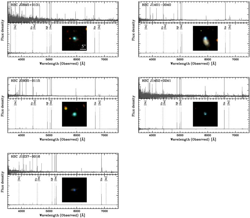
Figure 1: The newly identified $5$ EMPRESS EMPGs with their optical spectra and images. For each object the bottom panel shows the MagE spectrum arbitrary normalized based on the strong emission lines, while the top panels decreases the scale of the vertical axis by a factor of $20$ to see the weaker lines. The inserted panel presents $20^{\prime\prime}\times 20^{\prime\prime}$ $gri$ composite image from HSC centered on the EMPG core. North is up and east is to the left.

2.1.2 EMPRESS EMPGs: New data

Following the success of the machine-learning selection of EMPGs by EMPRESS (Kojima et al., 2020), we have expanded spectroscopic follow-up observations to increase the numbers of confirmed EMPGs and characterize their properties in a statistical manner.

The third spectroscopic observation was conducted with Magellan/MagE on UT 2021 February 10 in clear conditions with a seeing of $0.5$–$0.9^{\prime\prime}$. Ten EMPG candidates were selected for the follow-up from the HSC candidate catalog. We chose 7 from the catalog originally provided by Kojima et al. (2020), and the remaining 3 from a newly provided, enlarged EMPRESS sample. The new sample was based on an upgraded machine learning classifier with further metal-poor EMPG training models (Z $=10^{-3}$–$0.01$ $Z_{\odot}$; based on photoionization models from Nakajima et al. 2018b) and the latest HSC-SSP DR (S20A; Aihara et al. 2018). In addition to the HSC candidates, we observed 4 previously known (E)MPGs ($12+\log({\rm O/H})$ $=7.4$–$8.0$; Kniazev et al. 2003; Izotov et al. 2012b) selected from SDSS, to examine the kinematics of low-mass galaxies (Xu et al., 2021). Full details of the observation and data reduction procedures are presented in a companion paper of (Xu et al., 2021). Briefly, we found nine out of the ten HSC candidates in which we identified multiple emission lines over the wavelength range of $\lambda_{\rm obs}=3500$–$10000$ Å that are suggestive of metal-poor galaxies at $z\lesssim 0.05$. In this paper, we report the properties of the nine new galaxies of HSC as well as the four SDSS galaxies (hereafter, MagE sources).

Table 1 lists the key line intensities normalized by H$\beta$ and their $1\sigma$ errors for the $13$ MagE sources. We measure the flux of each of the lines by fitting a Gaussian profile plus a constant continuum. The measured fluxes are then corrected for Galactic extinction based on the Schlafly & Finkbeiner (2011)’s map as well as the extinction curve of Cardelli et al. (1989). We use the Balmer lines of H$\alpha$, H$\beta$, H$\gamma$, and H$\delta$ to estimate the dust attenuation by simultaneously fitting the fluxes assuming the Calzetti et al. (2000)’ attenuation curve. We do not correct for the potential stellar absorption around the Balmer lines which would be negligible ($\sim 1$–$2$ Å in metal-poor galaxies; e.g., Izotov et al. 2012a) for our sources with very large EWs of emission lines (EW(H$\beta$) $\sim 100$–$550$ Å).

Table 2: Physical properties of MagE sources

ID	EW(H$\beta$)	$T_{e}$(O iii)	$N_{e}$(O ii)	12+log(O/H)
	(Å)	($10^{3}\,$K)	(cm-3)
HSC J0845+0131	$220.7\pm 30.0$	$18.4\pm 2.5$	–	$7.35\pm 0.13$
HSC J0912-0104	$142.9\pm 32.4$	–	–	–
HSC J0935-0115	$266.5\pm 9.7$	$20.1\pm 1.0$	$30^{+100}_{-30}$	$7.17\pm 0.07$
HSC J1210-0103	$180.7\pm 18.1$(†)	–	–	–
HSC J1237-0016	$225.2\pm 19.9$	$19.3\pm 1.0$	$20^{+220}_{-20}$	$7.55\pm 0.08$
HSC J1401-0040	$133.5\pm 4.7$	$17.3\pm 0.9$	$110^{+70}_{-60}$	$7.64\pm 0.06$
HSC J1407-0047	$98.9\pm 9.0$	–	$130^{+350}_{-130}$	–
HSC J1411-0032	$288.4\pm 24.7$	$13.0\pm 0.5$	$200^{+100}_{-80}$	$8.12\pm 0.06$
HSC J1452+0241	$550.8\pm 6.4$(†)	$19.1\pm 2.2$	$<710$	$7.21\pm 0.12$
SDSS J1044+0353	$307.4\pm 8.8$	$19.1\pm 0.5$	$170^{+110}_{-90}$	$7.45\pm 0.04$
SDSS J1253-0312	$226.8\pm 8.0$	$13.3\pm 0.4$	$350^{+50}_{-50}$	$8.09\pm 0.06$
SDSS J1323-0132	$227.2\pm 6.2$	$18.1\pm 0.6$	$310^{+150}_{-120}$	$7.74\pm 0.05$
SDSS J1418+2102	$269.7\pm 5.2$	$17.6\pm 0.3$	$40^{+50}_{-40}$	$7.64\pm 0.04$

Note. — EW(H$\beta$) are given at the rest-frame value. EWs are determined based on the spectra except for those with (${\dagger}$). (${\dagger}$) Because their continuums are not detected in the spectra, EW(H$\beta$) are estimated from the photometrically inferred EW(H$\alpha$) divided by the typical EW ratio of $5.47$ (see §4.4). Metallicities are based on the direct $T_{e}$ method and given for those with a [O iii]$\lambda 4363$ detection. Upper-limit of $N_{e}$ is given at the $1\sigma$ level. For HSC J0845+0131, $N_{e}$ is constrained to be $<130$ cm^-3 at the $2\sigma$ level.

One of the key properties to characterize our sources is gas-phase metallicity. We identify the temperature-sensitive line of [O iii]$\lambda 4363$ in $10$ of the $13$ sources. For the $10$ objects, $6$ of which are HSC-selected, we determine the oxygen abundance using the direct $T_{e}$ method and use it as a proxy for gas-phase metallicity. We first estimate electron number densities and electron temperatures using getTemDen, a package of a Python tool PyNeb (Luridiana et al., 2015). We use [O ii]$\lambda\lambda 3726/3729$ doublet ratio to estimate the density of O⁺ ions ($N_{e}$(O ii)), and assume a homogeneous density in the entire gas. The density varies from $20$ to $350$ cm^-3 for the nine objects whose [O ii] doublet are significantly detected. The [O iii]$\lambda\lambda 4363/5007$ ratio is then input together with the measured density into getTemDen to derive the electron temperature of O²⁺ zone ($T_{e}$(O iii)). For the 2 sources without a direct measurement of density, we assume a typical value of $100$ cm^-3, consistent with the upper-limits of $N_{e}$ for both of the sources. We have also confirmed the density assumption has little impact on the derived metallicity values ($\Delta log$(O/H) $<0.01$ dex) by changing the assumed density from $1$ to $1000$ cm${-3}$. The temperature of O⁺ zone, $T_{e}$(O ii), is extrapolated from $T_{e}$(O iii) employing the prescription of Izotov et al. (2006b). We derive the abundances of O⁺$/$H⁺ with the [O ii]$\lambda\lambda 3726,3729$ ([O ii]$\lambda 3727$ hereafter as a sum of the doublet) to H$\beta$ and $T_{e}$(O ii), and O²⁺$/$H⁺ with the [O iii]$\lambda\lambda 4959,5007$ to H$\beta$ and $T_{e}$(O iii) using the PyNeb package getIonAbundance. For a possible higher ionization abundance of O³⁺$/$H⁺, we follow the approximation given by Izotov et al. (2006b). Specifically, we add the O³⁺ component in the calculation if the Heii$\lambda 4686$ emission line is detected. The contribution is small for the strongest case (O³⁺$/$(O⁺+O²⁺) $<0.012$) which is consistent with the previous EMPG studies. The measured oxygen abundances as well as $T_{e}$(O iii) and $N_{e}$(O ii) are summarized in Table 2. Five of the 6 HSC-selected EMPG candidates have a metallicity below the $10$ % solar value ($12+\log({\rm O/H})$ $<7.69$) and are thus confirmed being EMPGs. The spectra and optical images for the newly identified EMPRESS-EMPGs are illustrated in Figure 1. One source, J1411-0032, is turned out to be slightly metal-enriched system as similarly identified in earlier studies of EMPRESS (Kojima et al. 2020; Isobe et al. 2021), and added to the MPG catalog. For the other three HSC-selected EMPG candidates, the non-detection of [O iii]$\lambda 4363$ is still consistent with a metal-poor (i.e., high electron temperature) gas due to the rather faint nature. Indeed, their metallicities are indirectly inferred to be as low as those of EMPGs ($12+\log({\rm O/H})$ $=7.1$–$7.4$) based on the empirical metallicity indicators of R23-index and the upper-limit of N2-index (optimized for sources with EW(H$\beta$)=$100$–$200$ Å; see §3.2). Future deep spectroscopy will reveal the properties in more details for the unconfirmed candidates.

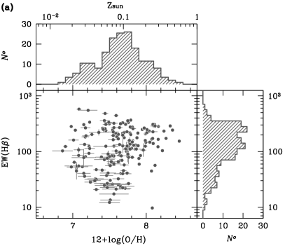
(a)

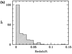
(b)

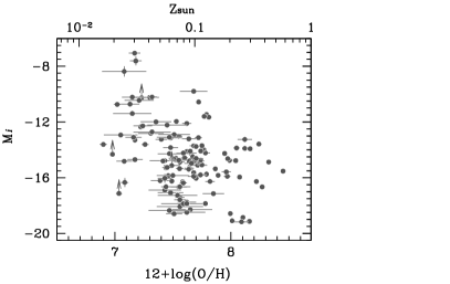
(c)

(d)

Figure 2: (a) Scatter plot matrix showing the distributions of $12+\log({\rm O/H})$, EW(H$\beta$), and $M_{i}$ for the compiled metal-poor galaxies (both EMPGs and MPGs) in this paper. (b) Redshift distribution of the compiled (E)MPGs. We compile EMPGs (i.e., $12+\log({\rm O/H})$ $<7.69$) as complete as possible in the local universe ($95$ % are at $z<0.05$), while include the MPGs only when found in the EMPG literature.

In addition, a further spectroscopic follow-up has been conducted under EMPRESS and will be detailed in a series of forthcoming papers (e.g., Nishigaki et al. 2022 in prep.). In this paper, we additionally exploit the results of $3$ new EMPGs from the latest observations.

In summary, there are 8 EMPGs and one MPG newly identified in the EMPRESS sample. These 9 EMPRESS galaxies as well as the 4 SDSS galaxies (2 EMPGs and 2 MPGs) whose properties are re-measured with the MagE spectra are added to our sample and used for the following analysis. We do not use the remaining 3 faint HSC galaxies in this paper, although their strong emission lines indicate they are as metal-poor as EMPGs. This spectroscopic observation thus re-confirms the ability of EMPRESS to select EMPGs in the local universe from the photometric catalog.

2.1.3 Other EMPGs

In addition to the (E)MPGs provided by EMPRESS, we compile observations of comparably low-metallicity objects from the literature that have a firm determination of gas-phase metallicity based on [O iii]$\lambda 4363$. We find $154$ objects in total, without any duplication, in the literature (Kniazev et al., 2003; Thuan & Izotov, 2005; Pustilnik et al., 2005; Izotov et al., 2006a, 2009, 2012a, 2012b, 2018b, 2019b, 2020, 2021; Izotov & Thuan, 2007; Guseva et al., 2007; Pustilnik et al., 2010; Skillman et al., 2013; Hirschauer et al., 2016; Sánchez Almeida et al., 2016; Hsyu et al., 2017) which include isolated galaxies such as emission line galaxies and blue compact dwarfs as well as metal-poor clumps and Hii-regions in a nearby galaxy. Only the sources with a reliable determination of oxygen abundance have been collected, with the direct $T_{e}$ method using a suite of the optical oxygen and hydrogen emission lines as for the EMPRESS sources (§2.1.2). Some nearby objects lack [O ii]$\lambda 3727$ especially in the SDSS spectra. For these objects, the O⁺$/$H⁺ abundance has been derived with the [O ii]$\lambda\lambda 7319,7330$. Sources with a large uncertainty of metallicity, $\Delta$ log(O/H) $>0.2$, have been removed from the compilation. For those without line flux/EW values reported in the literature (Kniazev et al., 2003; Sánchez Almeida et al., 2016), we have used the SDSS Data Release 16 SkyServer to retrieve the spectroscopic data. Among the $154$ compiled objects, $87$ sources present a metallicity below $12+\log({\rm O/H})$ $=7.69$ and are classified as EMPGs. The remaining, relatively low-metallicity objects ($12+\log({\rm O/H})$ $=7.7$–$8.4$) are MPGs that are supplementarily provided from the same literature as used for the EMPG compilation. The MPG subsample is therefore not complete in terms of metallicity but just served as a reference sample.

In summary, our sample contains $103$ EMPGs and $82$ MPGs ($N^{o}=185$ in total), increasing the sample size of EMPGs by a factor of three as compared to that of previous work (e.g., Nagao et al. 2006). We note that no obvious active galactic nuclei (AGN) activity is identified in the compiled (E)MPG sample based on the BPT diagram (Kauffmann et al., 2003). Although we may not fully exclude the possibility of metal-poor AGN in the sample with the BPT diagram according to the photoionization predictions (Kewley et al., 2013), we assume no AGN in the sample in the following analysis. Figure 2 (a) presents the distributions of metallicity, EW(H$\beta$), and $i$-band absolute magnitude $M_{i}$ for the compiled sources. We derive $M_{i}$ based on the $i$- or $z$-band broadband photometric data of HSC or SDSS, in addition to the luminosity distance. We choose the broadband which is free from an intense H$\alpha$ emission for each of the objects (see §4.4 for more details). The EMPGs cover large parameter spaces of $M_{i}$ from $-19$ to $-7$ and EW(H$\beta$) from $10$ to $600$ Å, i.e., wide ranges of stellar mass and specific star-formation rate, respectively. Assuming a mass to optical luminosity relation typically seen in (E)MPGs (Kojima et al., 2020; Xu et al., 2021), the Kennicutt (1998) relation, and a Chabrier (2003) initial mass function, the ranges correspond to the stellar masses of $10^{8}$ $M_{\odot}$ down to below $10^{4}$ $M_{\odot}$, and to the specific star-formation rates of a few Gyr^-1 up to $\sim 200$ Gyr^-1. Notably, the EMPRESS survey enlarges the sample of the largest EW(H$\beta$) (E)MPGs (e.g., see EW(H$\beta$) of the HSC-selected objects in Table 2). Figure 2 (b) shows the redshift distribution of the sample confirming that most of the (E)MPGs ($95$%̇) are found at $z<0.05$. Their UV properties are also derived and discussed later in this paper (§4).

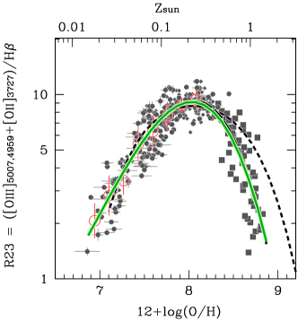
(a)

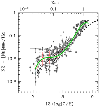
(b)

Figure 3: Relationship between metallicity and the strong line ratios of R23-index (left) and N2-index (right). Our compiled (E)MPGs are shown with gray filled circles (individual) and red open circles (binned average, with the standard deviation of the binned distribution as the error). Gray filled squares denote stacked SDSS spectra in the high-metallicity regime (Curti et al., 2017, 2020). Small gray diamonds are metal-poor galaxies compiled by Nagao et al. (2006) just for a reference (i.e., not used for the following best-fit function). All the measurements of metallicity are done in a consistent manner based on the direct $T_{e}$ method. Green curve presents our best-fit function, whereas the black short-dashed and long-dashed curve illustrates the function of Maiolino et al. (2008) and Curti et al. (2017, 2020), respectively.

2.2 Stacked SDSS Galaxies

To compensate the high-metallicity range in determining the metallicity diagnostics (§3), we exploit the analyses of Curti et al. (2017, 2020) which are based on $120,000$ galaxies’ spectra from SDSS. Sources that are dominated by an AGN activity are excluded from the sample based on the BPT diagram (Kauffmann et al., 2003). The authors stack SDSS spectra in bins of strong line ratios to detect the [O iii]$\lambda 4363$ in a statistical manner and determine the metallicity based on the direct $T_{\rm e}$ method. Each bin contains $10-\sim 6000$ galaxies for the stacking analysis. The resulting stacked spectra show metallicities ranging from $12+\log({\rm O/H})$$=8.1$ to $\sim 8.9$.

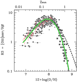
(a)

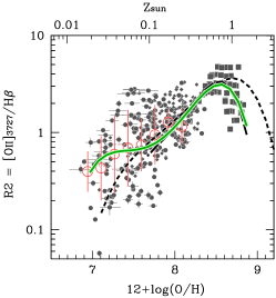
(b)

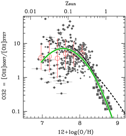
(c)

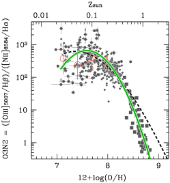
(d)

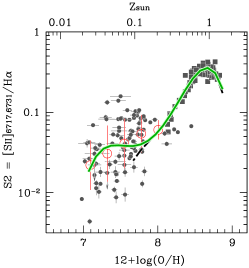
(e)

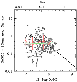
(f)

Figure 4: Same as Figure 3 but for the line ratios of R3, R2, O32, O3N2, S2, and Ne3O2 (from top left to bottom right).

3 Strong line diagnostics of metallicity

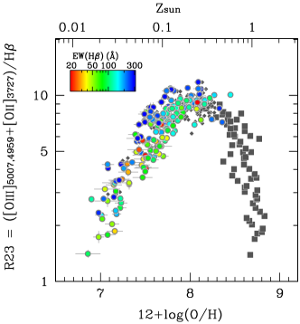
(a)

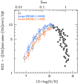
(b)

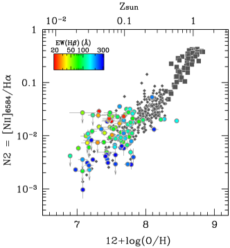
(c)

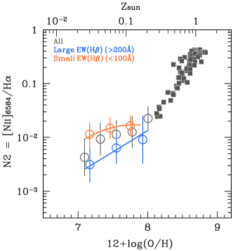
(d)

Figure 5: Same as Figure 3 but highlighting that the dispersion in the indicator of R23-index (top) and N2-index (bottom) is correlated with EW(H$\beta$). In the left panels, our compile (E)MPGs are color-coded according to EW(H$\beta$). Their binned average relationships are presented in the right panels, where blue and orange open circles are based on the Large and Small EW(H$\beta$) objects (EW $>200$ Å and $<100$ Å), respectively, while gray open circles are based on the full sample of the compiled (E)MPGs. The best-fit functions to the Large and the Small EW(H$\beta$) subsamples are over-plotted with the same color-code.

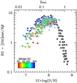
(a)

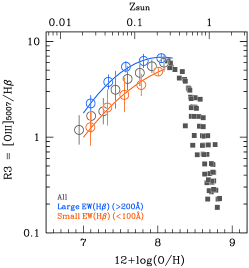
(b)

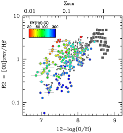
(c)

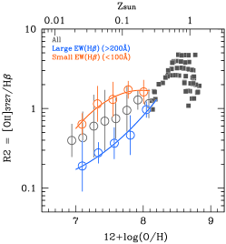
(d)

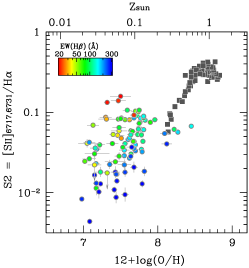
(e)

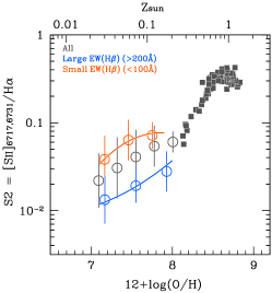
(f)

Figure 6: Same as Figure 5 but for the line ratios of R3, R2, and S2 (from top to bottom).

(a)

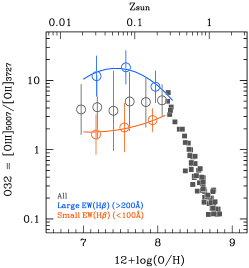
(b)

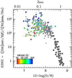
(c)

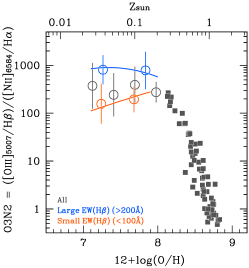
(d)

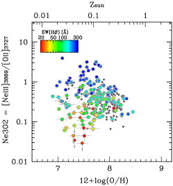
(e)

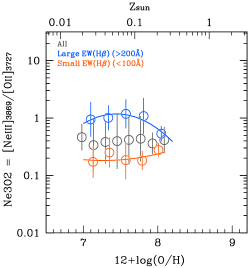
(f)

Figure 7: Same as Figure 5 but for the line ratios of O32, O3N2, and Ne3O2 (from top to bottom).

3.1 Revisiting Diagnostics over
$12+\log({\rm O/H})$ $\simeq 6.9-8.9$

Our compiled sample containing quite a few numbers of EMPGs ($\times 3$ larger than the previous work; e.g., Nagao et al. 2006) with an accurate metallicity measurement serves as a good reference for checking and improving the empirical metallicity diagnostics at the low-metallicity regime. Figure 3 illustrates the relationship of R23- and N2-index as a function of metallicity. Our compiled sources (gray circles) shape a tight relationship for each of the indices, remarkably for R23-index, at the low metallicity regime. The short-dashed and long-dashed curve is provided by Maiolino et al. (2008) and Curti et al. (2017, 2020), respectively, and the green curve shows our best-fit function (as detailed below). The two previous studies are complementary to each other; Maiolino et al. (2008) make use of the individual low-metallicity galaxies but lack data-points at high metallicity range with the direct $T_{e}$ method. On the other hand, Curti et al. (2017, 2020) obtain the relations at such a high-metallicity regime based on the direct $T_{e}$ method by stacking SDSS spectra (§2.2), but lack enough metal-poor galaxies.

Therefore, as a first step in this section, we present the best-fit functions over the full metallicity range of $12+\log({\rm O/H})$ $\simeq 6.9$ up to $8.9$ based fully on the direct $T_{e}$ method. We use our compiled sample of EMPGs $+$ MPGs ($12+\log({\rm O/H})$ $=6.9$–$8.2$; §2.1) in addition to the Curti et al. (2017, 2020)’s stacked result to compensate the high metallicity regime ($12+\log({\rm O/H})$ $=8.1$–$8.9$; §2.2). We confirm in Figure 3 that the two independent samples are smoothly connected at the intersection of $12+\log({\rm O/H})$ $\sim 8.0$. Following the previous studies, we adopt the functional form:

$$\log R=\Sigma_{n=0}^{N}c_{n}x^{n}$$ (1)

to derive the best-fit, where $\log R$ is the logarithm of the strong line ratio (e.g., R23 and N2-index), and $x$ is the metallicity relative to solar (i.e., $x=\log(Z/Z_{\odot})=12+\log({\rm O}/{\rm H})-8.69$). We bin the compiled (E)MPGs to obtain average line ratios for a given metallicity range (red open circles in Figure 3; Table 3 for the “All” sample) and use them to perform the least squares fitting with the stacked data-points of Curti et al. (2017, 2020) without any weighting. For the binning we only use the individual (E)MPGs with a firm measurement of line ratio and do not count those with a lower-/upper-limit of line ratio of interest. We employ the polynomial orders of $N=2$, $3$, and $4$ in Equation (1), and choose the best-fit for each of the indices from the three functional forms which minimizes the dispersions along with both the $12+\log({\rm O/H})$ and the line ratio directions. Note that we use the individual (E)MPGs rather than the binned average ones for calculating the dispersions. The coefficients as well as the $1\sigma$ uncertainties of the best-fit are given in Table 4 for each indices based on the “All” sample. As expected, our best fit-functions show good agreements with those of Maiolino et al. (2008) in the low-metallicity and Curti et al. (2017, 2020) at the high-metallicity regime.

3.2 Scatters in the diagnostics

R23-index is confirmed to work as a good metallicity indicator with the metallicity uncertainty of $0.14$ dex over the range of $12+\log({\rm O/H})$ $=6.9-8.9$ (Table 4). Although N2-index works as accurately as R23-index for galaxies in the high-metallicity range, we recognize large scatters as large as $\Delta\log$(O/H) $\sim 0.4$ dex in the relation in the metal-poor regime. A more or less similar scatter of the line ratio is also found in Figure 4 when other famous indicators are chosen as a function of metallicity: [O iii]$\lambda 5007$$/$H$\beta$ (R3), [O ii]$\lambda 3727$$/$H$\beta$ (R2), [O iii]$\lambda 5007$$/$[O ii]$\lambda 3727$ (O32), R3$/$N2 (O3N2), [S ii]$\lambda\lambda 6717,6731$$/$H$\alpha$ (S2), and [Ne iii]$\lambda 3869$$/$[O ii]$\lambda 3727$ (Ne3O2). Weird concave down features found in the best-fit in O32- and O3N2-index as well as plateau-like behaviors in R2-, S2-, and Ne3O2-index illustrate their weak dependence on metallicity in the low metallicity regime with the current function forms (see also their large uncertainties of $\Delta\log$(O/H) in Table 4). We note that this paper cannot fully address scatters in the high-metallicity range, as we only have the averaged line ratios based on the stacked SDSS spectra (see also §3.4). In the following, we explore and discuss the scatters in the low-metallicity regime using our compiled (E)MPG sample.

As found in N2-index, a large scatter appears particularly associated with the line ratios using singly-ionized, low-ionization lines. We thus speculate this would be caused by a variation of ionization state in the ISM for a given metallicity, such as ionization parameter and ionizing radiation field. Indeed, Pilyugin & Grebel (2016) demonstrate that, for a given metallicity, N2-index tends to become lower with the excitation parameter (=[O iii]$/$([O ii]$+$[O iii])). The excitation parameter and O32-index are famous probes of the ionization parameter (e.g., Kewley & Dopita 2002; Nakajima & Ouchi 2014), and useful to correct for such an effect of ionization state on the metallicity indicators (see also Pilyugin & Thuan 2005; Kewley & Dopita 2002; Izotov et al. 2019a). Although it is recommended to adopt these direct indicators of ionization parameter as a correction factor, it will not be always possible to obtain such multiple emission lines probing both high and low ionization gas from distant galaxies. Because our main purpose of this work is to provide metallicity diagnostics that will be practical and useful even when limited sets of emission lines are available, we re-examine the scatters in the indices using a different observable quantity, which is easy-to-obtain and a good probe of the ionization state. Among several observables, we consider EW(H$\beta$) (or equivalently EW(H$\alpha$)) is best-suited for this purpose for the following reasons. First, O32-index is known to be positively correlated with specific star-formation rate (e.g., Nakajima & Ouchi 2014; Sanders et al. 2016), which should be proportional to EWs of H$\beta$ and H$\alpha$ by definition. Indeed, our (E)MPGs shape a tight positive correlation between O32-index and EW(H$\beta$). Second, as will be illustrated in §4.4, $\xi_{\rm ion}$, a gauge of the hardness of the ionizing radiation field, is primarily controlled by EW(H$\beta$), such that it becomes larger as EW(H$\beta$) increases. Finally, as compared to the ionization/excitation parameters, O32-index, and $\xi_{\rm ion}$, EW(H$\beta$) is a direct observable quantity and easy to get from high-redshift galaxies with JWST, and reliably measured without being affected by dust extinction and other assumptions. We expect at least either of H$\beta$ and H$\alpha$ is available when using the metallicity indicators, and EW(H$\alpha$) can be translated into EW(H$\beta$), such that EW(H$\alpha$) $=5.47\times$ EW(H$\beta$) following a typical relationship (Kojima et al., 2020). Therefore, we expect we can use EW(H$\beta$) to probe the degree of ionization state in ISM of distant galaxies in a practical manner. Moreover, a presence of diffuse ionized gas (DIG) can influence the line ratios, especially of the low-ionization lines (Zhang et al., 2017; Sanders et al., 2017). This effect can also be quantified by EW(H$\beta$), as the fraction of emission from DIG is thought to decrease with increasing star-formation intensity (Oey et al., 2007).

(a)

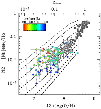
(b)

Figure 8: Photoionization model predictions of R23-index (left) and N2-index (right) and comparisons with the observations (Figure 5). The black grid illustrates the photoionization models based on the binary evolution SEDs (BPASS-300bin; Nakajima et al. 2018b). The dashed-curves present model tracks with an ionization parameter $\log\,U$ from $-3.5$ (thin) to $-0.5$ (thick) with a step of $0.5$ dex. Only the gas-phase oxygen abundance is counted for the models (i.e., after removing the depleted component onto dust grains) in the abscissa axis to be directly compared with the observations. The gas density is fixed to $100$ cm^-3. The models explain the scatter and its correlation with EW(H$\beta$) by changing the ionization parameter in a consistent manner for each of the indicators.

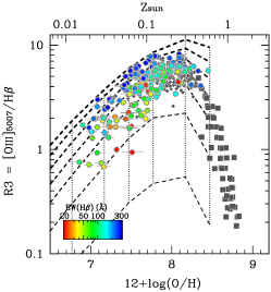
(a)

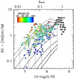
(b)

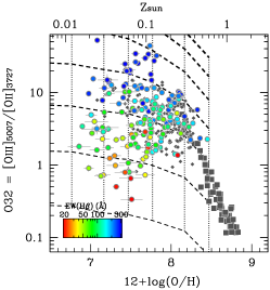
(c)

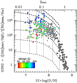
(d)

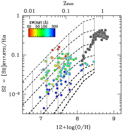
(e)

(f)

Figure 9: Same as Figure 8 but for the line ratios of R3, R2, O32, O3N2, S2, and Ne3O2 (from top left to bottom right).

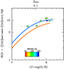
(a)

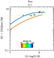
(b)

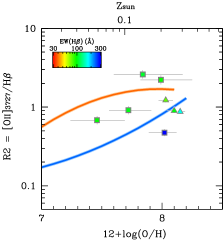
(c)

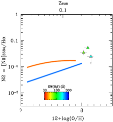
(d)

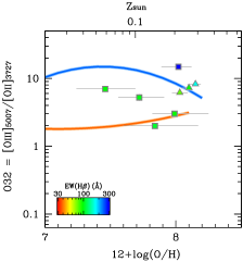
(e)

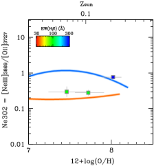
(f)

Figure 10: Relationships between metallicity and the strong line ratios of R23, R3, R2, N2, O32, and Ne3O2 (from top left to bottom right) and their dependence on EW(H$\beta$) to be compared with observations of $z=2-3$ galaxies. Squares show galaxies with a detection of [O iii]$\lambda 4363$ (Christensen et al., 2012; Sanders et al., 2020), and triangles represent galaxies with O iii]$\lambda\lambda 1661,1666$ (Erb et al., 2010; Steidel et al., 2014). The symbols are color-coded based on EW(H$\beta$) as shown in the legend. We assume the theoretical [O iii]$\lambda 5007/4959$ line ratio of $2.98$ (Storey & Zeippen, 2000) to correctly derive R23 and R3 as defined in this paper, if only the sum of the two lines or only the $5007$ component is listed in the original literature. The curves show the relationships derived in this paper; based on the (E)MPG subsamples of Large EW(H$\beta$) (blue) and Small EW(H$\beta$) (orange).

Figure 5 (Left) shows the same diagnostics of R23 and N2 as in Figure 3 but our compiled EMPGs + MPGs are color-coded with EW(H$\beta$). To clarify the dependence on EW(H$\beta$), we split the sample into three subsamples, “Small EW” ($<100$ Å), “Medium EW” ($100$–$200$ Å), and “Large EW” ($>200$ Å), and give the binned average results for the Small and Large EW subsamples in the right panels. Note again that this paper explores the EW(H$\beta$) dependence only in the low metallicity regime ($12+\log({\rm O/H})$ $\lesssim 8.0$). We see a clear trend that the scatter in the indices is correlated with EW(H$\beta$). For a given metallicity, sources with a larger EW(H$\beta$) tend to present a larger R23 and a smaller N2 value. This can be interpreted as a result of large variation of ionization condition in metal-poor clouds, i.e., the ionization parameter and/or the hardness of the ionizing spectrum among galaxies with a comparable metallicity (Pilyugin & Grebel, 2016). The trend in N2-index is straightforward, while that of R23 needs more careful explanations because it uses a sum of singly and doubly ionized lines in the numerator. Figures 6 and 7 summarize the dependence of the other metallicity indicators on EW(H$\beta$). We confirm the correlation between the scatters in the metallicity indicators and EW(H$\beta$), such that higher ionization lines ([O iii], [Ne iii]) tend to be stronger with EW(H$\beta$) for a given metallicity than lower ionization lines ([O ii], [N ii], [S ii]) including the hydrogen recombination lines. Because the binned average relationships of the Large EW sample are more similar to the earlier work showing relatively strong powers of these line ratios as metallicity indicators at the low metallicity range (e.g., O32- and Ne3O2-index; Maiolino et al. 2008), the weak metallicity-dependence we obtain for the “ALL” sample, in contrast to the earlier work, are thought to be due to the presence of objects with a low ionization condition. The correlation between the metallicity and ionization state will be further discussed later (§3.4). As for R23-index, it is relatively strong against the variation of the ionization state by tracing both low and high ionization gas, resulting in the smallest metallicity dispersion ($0.14$ dex). In the low metallicity regime, R23-index becomes dominated by R3-index as O32 becomes larger than unity. We thus see a similar trend of EW(H$\beta$) as seen in R3-index but slightly milder in R23-index.

The binned average relationships of the metallicity indicators for each of the subsamples are summarized in Table 3, and their best-fit functions can be reproduced within the metallicity range and with the coefficients given in Table 4. We fix $N=2$ for the best-fit functions for the subsamples. Table 4 also lists the standard deviations of $12+\log({\rm O/H})$ as typical uncertainties for each of the indicators and subsamples. For example, below $12+\log({\rm O/H})$ $\leq 7.69$, the uncertainty of metallicity using R3-index (All) is 0.21 dex, which becomes as small as 0.10 dex (i.e., by a factor of 2) if the subsample’s best-fits are employed. In a similar way, we confirm the accuracy of the metallicity indicators becomes significantly improved if the best-fit function depending on EW(H$\beta$) is used. Although the indicators using a high ionization line divided by a low ionization line, O32, O3N2, and Ne3O2, show a smaller improvement in the standard deviation than the other indicators, it is mostly due to the larger impact of ionization condition on these line ratios even within the subsamples of EW(H$\beta$) $>200$ Å and $<100$ Å (Fig. 7). This is the current limitation. Another practical note is that we recommend to use the best-fit relationships of the Large and Small EW subsample for sources with EW(H$\beta$) $>200$ Å and $<100$ Å, respectively, and interpolate the two solutions for sources with EW(H$\beta$) in between $100$ and $200$ Å.

3.3 Comparisons with photoionization models

To confirm the variation of ionization condition on the strong line diagnostics, we compare the results with photoionization models. We exploit the CLOUDY photoionization modeling as detailed in Nakajima et al. (2018b). Briefly, we refer to the models of star-forming galaxies using binary evolution SEDs of “BPASS-300bin” (v2; Eldridge et al. 2017). For this comparison, we slightly expand the original BPASS model grid of Nakajima et al. (2018b) to cover the extremely low metallicity down below the $0.01$ $Z_{\odot}$ adopting the same assumptions such as the abundance ratios and the relationship between stellar and gas-phase metallicities. The ionization parameter is varied to assess the impact of changing the ionization condition on the emergent strong line ratios. The gas density is fixed to a fiducial value of $100$ cm^-3. One caveat here is that the metallicity in the original CLOUDY models counts elements depleted onto dust grains in addition to those in gas-phase in the ionized nebula. On the other hand, the metallicities observationally derived based on the direct $T_{e}$ method trace the oxygen abundances only in gas-phase (O⁺/H⁺ + O²⁺/H⁺ + O³⁺/H⁺; see 2.1.2). To directly compare the models with the observations, we subtract the depleted component from the total oxygen abundance for each of the models using the adopted depletion factor of $0.6$ for oxygen.

In Figures 8 and 9, we present the comparisons of the metallicity diagnostics between the photoionization predictions and the observations. The models reproduce the scatters as well as the trend observed with EW(H$\beta$) for a given metallicity by changing the ionization parameter within a reasonable range of $\log\,U$ from $-3.5$ to $-0.5$. The comparison demonstrates that we can substitute EW(H$\beta$) as a gauge of the degree of ionization in ISM, and that the metallicity indicators that do not use a sum of low and high ionization lines can be weak without any correction for the ionization state, as they cannot trace both low and high ionization gas, latter of which particularly exist widely in metal-poor clouds.

3.4 Implications

The non-negligible correlations seen in the metallicity indicators in terms of EW(H$\beta$), as a result of the difference in the degree of ionization state in the ISM, have some implications. First, it would be important to adopt the appropriate relationship following the EW of H$\beta$ (or H$\alpha$), rather than using the best-fit for the “All” sample blindly, to improve the accuracy of the derived metallicity based on these empirical relationships. Particularly, this would influence discussions of mass-metallicity relation and its star-formation rate dependency (e.g., Mannucci et al. 2010; Lara-López et al. 2010), because EW(H$\beta$) is a strong function of stellar mass and star-formation rate. Although R23-index is the best indicator which is the least affected by the difference of the ionization state among various popular indicators, there still remains a factor of $\sim 1.5$ difference in R23-index between the Large and Small EW subsamples for a given metallicity below $12+\log({\rm O/H})$ $\lesssim 8.0$. This corresponds to a systematic offset of metallicity as large as $\Delta\log({\rm O/H})$ $\sim 0.25$ dex for a given R23 value between the large ($>200$ Å) and small ($<100$ Å) EW(H$\beta$) objects. A worse case is to blindly use a ratio of high to low ionization emission line such as O32, O3N2, and Ne3O2 indicators which show a weak dependence to estimate the metallicity below $12+\log({\rm O/H})$ $\lesssim 8.0$ especially if EW(H$\beta$) is not available (Figure 4).

Another important practical caveat when using R23-index and R3-index is that two solutions would be arithmetically obtained for a given index value. One would need additional single-valued functions such as N2- and S2-index to resolve the degeneracy, and be recommended to correct for the ionization condition using our prescription if the low-metallicity value ($12+\log({\rm O/H})$ $\lesssim 8.0$) is the likely solution. O32-index can also provide a discriminatory power to prefer the low-metallicity solution if O32-index is larger than $\sim 3$. Moreover, the two solution nature of R23-index and R3-index results in the plateau region around $12+\log({\rm O/H})$ $\sim 8.0\pm 0.2$ which results in a difficulty in pinpointing the metallicity when the index value is close to the maximum value of $\sim 9$. Indeed, the uncertainties of metallicity indicator of R23-index and R3-index (EW-corrected) are $0.13-0.25$ dex and $0.18-0.30$ dex, respectively, in the metallicity range of $12+\log({\rm O/H})$ $\leq 8.1$ (Table 4). These values get significantly smaller, $0.09-0.12$ dex and $0.10-0.18$ dex, in the metallicity range of $12+\log({\rm O/H})$ $\leq 7.69$, i.e., only considering the low-metallicity branch apart from the plateau region. The single-valued functions (e.g., N2- and S2-index), with a correction of ionization condition, are suggested to be used together with R23-index and R3-index to help ease the difficulty around the plateau region.

A second implication is about the large variation found in the indicators using low-ionization lines and high-to-low ionization line ratios. As clarified in the comparison plot of photoionization models and O32, O3N2, and Ne3O2-index (Figure 9), the variation suggests a diverse ionization nature of ISM in metal-poor galaxies. This appears in contrast to the SDSS’s high-metallicity regime where a relatively tight anti-correlation exists between metallicity and ionization parameter (e.g., Andrews & Martini 2013; Sanders et al. 2020). Because the SDSS stacking in Curti et al. (2017) is performed by dividing the sample based on the location on the R3 vs. R2 plot, it implicitly follows the anti-correlation between the ionization parameter and metallicity typically found in the local universe, resulting in a tight relationship between metallicity and O32, O3N2, and Ne3O2-index (Curti et al., 2017). This is why the Large EW subsample looks more smoothly connected with the SDSS sample at $12+\log({\rm O/H})$ $\sim 8.0$, as the highly-ionized galaxies are preferentially included in the lowest-metallicity bins of SDSS. If a similar anti-correlation typically exists between the metallicity and ionization parameter in the low-metallicity regime, the indicators that present weak dependences on metallicity such as O32, O3N2, and Ne3O2-index would become more helpful as seen in the Large EW subsample and as proposed in the earlier work (Maiolino et al., 2008). At the moment, however, our compilation demonstrates that outliers do exist as found in the Small EW subsample, such as EMPGs with a modestly ionized ISM having a low EW(H$\beta$). A presence of DIG can also play a role in scattering the low EW(H$\beta$) objects toward larger values of the low-ionization line indices (Zhang et al., 2017; Sanders et al., 2017). Our prescription will be useful to alleviate these uncertainties and derive metallicities for objects including such outliers. Because the Small EW subsample tends to contain individual stellar clumps and Hii-regions resolved in near-by galaxies, our current compilation may bias the sample following the detection of [O iii]$\lambda 4363$. We would need a larger and more well-constructed (e.g., mass-limited) EMPG sample to address the typical ionization condition as a function of metallicity. At the high-metallicity regime, we also expect some deviations from the typical ionization parameter – metallicity relationship and hence some improvements of diagnostics by using EW(H$\beta$) (cf. Brown et al. 2016; Cowie et al. 2016; Sanders et al. 2017). However, this is beyond this paper’s scope as we would need different analyses including how the SDSS sample is binned and stacked.

Finally, the metallicity prescriptions with the EW(H$\beta$) dependence would be essential for high-redshift galaxy studies. Because higher-$z$ galaxies are thought to present a higher ionization parameter (e.g., Nakajima & Ouchi 2014), the typical relationships (i.e., without the EW(H$\beta$) correction) constructed based on the local galaxies’ ionization parameter – metallicity relation may cause a systematic uncertainty of metallicity at high-redshift. To test the utility of the new metallicity diagnostics for high-redshift galaxies, we use the $z=2-3$ galaxies whose metallicity is determined with the electron temperature. As compiled in Sanders et al. (2020), we collect $8$ galaxies in total at $z=1.7$–$3.6$, five of which present a detection of [O iii]$\lambda 4363$ (Christensen et al., 2012; Sanders et al., 2020), and the remaining three’s electron temperatures are determined with O iii]$\lambda\lambda 1661,1666$ (Erb et al., 2010; Steidel et al., 2014). Figure 10 shows the $z=2-3$ galaxies, color-coded with EW(H$\beta$), superposed on the metallicity indicators found in the local universe. Albeit with the small sample size, the $z=2-3$ galaxies appear to support the same dependence of the relationships on EW(H$\beta$). The single galaxy having a very large EW(H$\beta$) ($340$ Å) notably follows the functions constructed with the Large EW(H$\beta$) subsample in the local universe ($>200$ Å). The other $7$ galaxies have modest values of EW(H$\beta$) ($80-170$ Å), and indeed fall in between the Large and Small EW subsamples on the metallicity indicators’ plots, with a tendency that the second largest EW(H$\beta$) galaxy ($170$ Å) prefers the relationship of the Large EW(H$\beta$) subsample. We admit the current sample size and the individual metallicity measurement uncertainties for the existing data-points do not permit a conclusive discussion. Still, we can argue that we do not see any clear contradiction of the metallicity indicators and the EW(H$\beta$) dependence at different redshifts up to $z\sim 3$.

The result is also consistent with the tendency found in Bian et al. (2018). The authors derive the empirical relationships between metallicity and strong line ratios for the typical local star-forming galaxies of SDSS as well as for analogs of $z\sim 2$ galaxies which are selected in the local universe but based on the offset location on the N2 vs. R3 plot (i.e., [N ii] BPT diagram) as typically seen at $z\sim 2$ (see also Steidel et al. 2014; Shapley et al. 2015). Using stacked spectra for each of the $z=0$ and $2$ samples, the authors suggest similar systematic offsets in the metallicity indicators between $z=0$ and $\sim 2$ as identified in this study. This makes sense as the $z=2$ analogous sample is constructed based on the elevated R3 value for a given N2-index, and preferentially contain galaxies with a higher ionization parameter and/or a harder ionizing spectrum for a given metallicity which can be characterized by a large EW(H$\beta$). The evolution of galaxies on the [N ii] BPT diagram would thus be largely due to the evolution of ionized ISM conditions and caused by the evolution of EW(H$\beta$) with redshift (see also the discussion of Reddy et al. 2018a based on EWs of [O iii]).

In brief, we can argue that a correction of ionization condition would be important in determining metallicities based on the strong line ratios, and the new metallicity prescriptions we develop using the local galaxies can be applicable even for high-redshift galaxies. We believe our prescriptions using EW(H$\beta$) are practically useful as it is easy to get as compared to ionization parameter and $\xi_{\rm ion}$. This work demonstrates careful applications of the strong line ratios are necessary to discuss the chemical evolution of galaxies as a function of stellar mass and star-formation activity. Nevertheless, we understand the current sample size is too small to confirm the applicability of the indicators at high-redshift. The relationships at high-redshift as well as local universe need to be further tested and improved, if necessary, with the forthcoming large and sensitive spectroscopic surveys such as Subaru/PFS (Takada et al., 2014) and VLT/MOONS (Cirasuolo et al., 2014).

Table 3: Binned average relationships of line ratio as a function of metallicity based on Compiled (E)MPGs

Flux ratio	Sample	12+log(O/H)	log R
R23	All	$6.94$	$0.32\pm 0.10$
		$7.11$	$0.45\pm 0.11$
		$7.27$	$0.53\pm 0.08$
		$7.43$	$0.73\pm 0.10$
		$7.59$	$0.80\pm 0.09$
		$7.76$	$0.88\pm 0.08$
		$7.92$	$0.94\pm 0.04$
		$8.08$	$0.97\pm 0.06$
	Large EW	$7.10$	$0.51\pm 0.09$
		$7.33$	$0.72\pm 0.07$
		$7.57$	$0.89\pm 0.05$
		$7.81$	$0.95\pm 0.06$
		$8.05$	$1.00\pm 0.04$
	Medium EW	$6.99$	$0.32\pm 0.12$
		$7.25$	$0.43\pm 0.06$
		$7.51$	$0.77\pm 0.10$
		$7.77$	$0.89\pm 0.06$
		$8.03$	$0.95\pm 0.04$
	Small EW	$7.09$	$0.39\pm 0.11$
		$7.32$	$0.62\pm 0.12$
		$7.55$	$0.71\pm 0.09$
		$7.78$	$0.82\pm 0.07$
		$8.01$	$0.91\pm 0.03$
R2	All	$6.94$	$-0.40\pm 0.21$
		$7.11$	$-0.37\pm 0.33$
		$7.27$	$-0.22\pm 0.39$
		$7.43$	$-0.16\pm 0.39$
		$7.59$	$-0.13\pm 0.27$
		$7.76$	$-0.02\pm 0.30$
		$7.92$	$0.11\pm 0.12$
		$8.08$	$0.06\pm 0.18$
	Large EW	$7.10$	$-0.72\pm 0.32$
		$7.33$	$-0.56\pm 0.13$
		$7.57$	$-0.44\pm 0.20$
		$7.81$	$-0.34\pm 0.25$
		$8.05$	$-0.01\pm 0.10$
	Medium EW	$6.99$	$-0.40\pm 0.09$
		$7.25$	$-0.36\pm 0.19$
		$7.51$	$-0.03\pm 0.10$
		$7.77$	$0.08\pm 0.17$
		$8.03$	$0.14\pm 0.13$
	Small EW	$7.09$	$-0.20\pm 0.14$
		$7.32$	$0.06\pm 0.23$
		$7.55$	$0.12\pm 0.22$
		$7.78$	$0.24\pm 0.11$
		$8.01$	$0.21\pm 0.15$
R3	All	$6.94$	$0.07\pm 0.15$
		$7.11$	$0.22\pm 0.18$
		$7.27$	$0.27\pm 0.14$
		$7.43$	$0.49\pm 0.20$
		$7.59$	$0.61\pm 0.13$
		$7.76$	$0.67\pm 0.14$
		$7.92$	$0.74\pm 0.07$
		$8.08$	$0.78\pm 0.09$
	Large EW	$7.10$	$0.35\pm 0.09$
		$7.33$	$0.58\pm 0.08$
		$7.57$	$0.73\pm 0.06$
		$7.81$	$0.80\pm 0.07$
		$8.05$	$0.82\pm 0.05$
	Medium EW	$6.99$	$0.09\pm 0.15$
		$7.25$	$0.22\pm 0.06$
		$7.51$	$0.59\pm 0.11$
		$7.77$	$0.67\pm 0.10$
		$8.03$	$0.74\pm 0.07$
	Small EW	$7.09$	$0.10\pm 0.19$
		$7.32$	$0.31\pm 0.19$
		$7.55$	$0.44\pm 0.18$
		$7.78$	$0.55\pm 0.12$
		$8.01$	$0.69\pm 0.04$
O32	All	$6.97$	$0.58\pm 0.36$
		$7.19$	$0.61\pm 0.46$
		$7.40$	$0.56\pm 0.58$
		$7.62$	$0.69\pm 0.42$
		$7.84$	$0.69\pm 0.37$
		$8.06$	$0.71\pm 0.23$
	Large EW	$7.18$	$1.06\pm 0.29$
		$7.57$	$1.19\pm 0.24$
		$7.97$	$0.91\pm 0.23$
	Medium EW	$7.08$	$0.55\pm 0.20$
		$7.51$	$0.65\pm 0.23$
		$7.95$	$0.59\pm 0.24$
	Small EW	$7.17$	$0.22\pm 0.29$
		$7.55$	$0.32\pm 0.35$
		$7.93$	$0.43\pm 0.17$
N2	All	$7.09$	$-2.37\pm 0.35$
		$7.32$	$-2.03\pm 0.30$
		$7.55$	$-1.94\pm 0.27$
		$7.78$	$-1.90\pm 0.30$
		$8.01$	$-1.65\pm 0.23$
	Large EW	$7.17$	$-2.51\pm 0.34$
		$7.55$	$-2.20\pm 0.30$
		$7.93$	$-2.04\pm 0.45$
	Medium EW	$7.29$	$-2.00\pm 0.04$
		$7.56$	$-1.98\pm 0.18$
		$7.83$	$-1.81\pm 0.24$
	Small EW	$7.17$	$-1.94\pm 0.22$
		$7.46$	$-1.83\pm 0.20$
		$7.75$	$-1.78\pm 0.19$
O3N2	All	$7.12$	$2.57\pm 0.48$
		$7.41$	$2.38\pm 0.45$
		$7.69$	$2.59\pm 0.38$
		$7.98$	$2.44\pm 0.21$
	Large EW	$7.26$	$2.91\pm 0.30$
		$7.83$	$2.90\pm 0.39$
	Medium EW	$7.36$	$2.57\pm 0.28$
		$7.76$	$2.48\pm 0.31$
	Small EW	$7.24$	$2.20\pm 0.42$
		$7.68$	$2.29\pm 0.27$
S2	All	$7.09$	$-1.66\pm 0.31$
		$7.32$	$-1.51\pm 0.35$
		$7.55$	$-1.39\pm 0.31$
		$7.78$	$-1.27\pm 0.23$
		$8.01$	$-1.22\pm 0.12$
	Large EW	$7.17$	$-1.88\pm 0.27$
		$7.55$	$-1.72\pm 0.19$
		$7.93$	$-1.55\pm 0.23$
	Medium EW	$7.29$	$-1.57\pm 0.12$
		$7.56$	$-1.31\pm 0.17$
		$7.83$	$-1.21\pm 0.13$
	Small EW	$7.17$	$-1.42\pm 0.27$
		$7.46$	$-1.20\pm 0.23$
		$7.75$	$-1.15\pm 0.15$
Ne3O2	All	$6.98$	$-0.34\pm 0.23$
		$7.14$	$-0.47\pm 0.46$
		$7.30$	$-0.42\pm 0.38$
		$7.45$	$-0.40\pm 0.48$
		$7.61$	$-0.38\pm 0.43$
		$7.77$	$-0.36\pm 0.39$
		$7.93$	$-0.44\pm 0.19$
		$8.09$	$-0.39\pm 0.23$
	Large EW	$7.10$	$-0.03\pm 0.30$
		$7.33$	$0.00\pm 0.22$
		$7.57$	$0.07\pm 0.25$
		$7.81$	$0.03\pm 0.32$
		$8.05$	$-0.27\pm 0.14$
	Medium EW	$7.03$	$-0.37\pm 0.01$
		$7.28$	$-0.48\pm 0.23$
		$7.53$	$-0.47\pm 0.22$
		$7.78$	$-0.48\pm 0.24$
		$8.04$	$-0.48\pm 0.18$
	Small EW	$7.13$	$-0.76\pm 0.28$
		$7.35$	$-0.60\pm 0.26$
		$7.57$	$-0.73\pm 0.33$
		$7.79$	$-0.74\pm 0.17$
		$8.01$	$-0.56\pm 0.12$

Table 4: Coefficients for empirical metallicity diagnostics (Eq. 1)

Flux ratio	Sample	$c_{0}$	$c_{1}$	$c_{2}$	$c_{3}$	$c_{4}$	Range(†)	$\Delta\log R$(‡)	$\Delta\log({\rm O}/{\rm H})$(‡)
R23	All	$0.515$	$-1.474$	$-1.392$	$-0.274$	–	[6.9:8.9]	$0.10$	$0.14$
								$0.08$ ($0.10$)	$0.14$ ($0.13$)
	Large EW	$0.866$	$-0.515$	$-0.463$	–	–	[7.1:8.1]	$0.05$ ($0.06$)	$0.25$ ($0.09$)
	Medium EW(⋆)	$0.986$	$-0.178$	$-0.335$	–	–	[7.0:8.0]	$0.07$ ($0.10$)	$0.14$ ($0.12$)
	Small EW	$0.875$	$-0.313$	$-0.387$	–	–	[7.1:8.0]	$0.08$ ($0.08$)	$0.13$ ($0.10$)
R2	All	$0.429$	$-1.044$	$-4.586$	$-4.117$	$-1.145$	[6.9:8.9]	$0.27$	$0.38$
								$0.30$ ($0.34$)	$0.43$ ($0.45$)
	Large EW	$0.697$	$1.327$	$0.273$	–	–	[7.1:8.1]	$0.21$ ($0.21$)	$0.28$ ($0.30$)
	Medium EW(⋆)	$0.362$	$0.204$	$-0.147$	–	–	[7.0:8.0]	$0.16$ ($0.16$)	$0.23$ ($0.21$)
	Small EW	$-0.033$	$-0.732$	$-0.510$	–	–	[7.1:8.0]	$0.19$ ($0.21$)	$0.31$ ($0.26$)
R3	All	$-0.277$	$-3.182$	$-2.832$	$-0.637$	–	[6.9:8.9]	$0.16$	$0.23$
								$0.15$ ($0.18$)	$0.27$ ($0.21$)
	Large EW	$0.628$	$-0.660$	$-0.522$	–	–	[7.1:8.1]	$0.06$ ($0.06$)	$0.30$ ($0.10$)
	Medium EW(⋆)	$0.718$	$-0.297$	$-0.387$	–	–	[7.0:8.0]	$0.10$ ($0.11$)	$0.22$ ($0.13$)
	Small EW	$0.780$	$-0.072$	$-0.316$	–	–	[7.1:8.0]	$0.15$ ($0.17$)	$0.18$ ($0.18$)
O32	All	$-0.693$	$-2.722$	$-1.201$	–	–	[7.0:8.9]	$0.39$	$0.39$
								$0.45$ ($0.51$)	$0.45$ ($0.45$)
	Large EW	$-0.080$	$-2.008$	$-0.804$	–	–	[7.2:8.0]	$0.25$ ($0.25$)	$0.38$ ($0.42$)
	Medium EW(⋆)	$0.344$	$-0.525$	$-0.250$	–	–	[7.1:8.0]	$0.23$ ($0.19$)	$0.36$ ($0.35$)
	Small EW	$0.865$	$0.771$	$0.243$	–	–	[7.2:7.9]	$0.31$ ($0.35$)	$0.48$ ($0.56$)
N2	All	$-0.482$	$1.052$	$-3.979$	$-5.479$	$-1.904$	[7.1:8.9]	$0.24$	$0.40$
								$0.29$ ($0.28$)	$0.52$ ($0.50$)
	Large EW	$-1.309$	$0.826$	$0.014$	–	–	[7.2:7.9]	$0.31$ ($0.28$)	$0.38$ ($0.35$)
	Medium EW(⋆)	$0.375$	$3.642$	$1.358$	–	–	[7.3:7.8]	$0.20$ ($0.15$)	$0.15$ ($0.15$)
	Small EW	$-2.181$	$-0.943$	$-0.532$	–	–	[7.2:7.8]	$0.19$ ($0.20$)	$0.35$ ($0.33$)
O3N2	All	$0.226$	$-4.710$	$-2.138$	–	–	[7.1:8.9]	$0.42$	$0.34$
								$0.49$ ($0.51$)	$0.44$ ($0.43$)
	Large EW	$2.126$	$-1.229$	$-0.456$	–	–	[7.3:7.8]	$0.34$ ($0.32$)	$0.38$ ($0.39$)
	Medium EW(⋆)	$0.033$	$-4.540$	$-2.020$	–	–	[7.4:7.8]	$0.29$ ($0.23$)	$0.37$ ($0.37$)
	Small EW	$2.786$	$0.396$	$-0.043$	–	–	[7.2:7.7]	$0.30$ ($0.32$)	$0.40$ ($0.38$)
S2	All	$-0.452$	$-0.297$	$-5.262$	$-5.881$	$-1.882$	[7.1:8.9]	$0.24$	$0.40$
								$0.30$ ($0.31$)	$0.50$ ($0.48$)
	Large EW	$-0.788$	$1.097$	$0.239$	–	–	[7.2:7.9]	$0.20$ ($0.20$)	$0.35$ ($0.37$)
	Medium EW(⋆)	$-0.456$	$0.959$	$0.148$	–	–	[7.3:7.8]	$0.14$ ($0.15$)	$0.22$ ($0.25$)
	Small EW	$-1.561$	$-1.066$	$-0.635$	–	–	[7.2:7.8]	$0.21$ ($0.23$)	$0.29$ ($0.29$)
Ne3O2	All	$-0.317$	$0.161$	$0.070$	–	–	[7.0:8.1]	$0.39$	$0.66$
								$0.39$ ($0.44$)	$0.66$ ($0.60$)
	Large EW	$-1.240$	$-2.106$	$-0.846$	–	–	[7.1:8.1]	$0.25$ ($0.26$)	$0.36$ ($0.40$)
	Medium EW(⋆)	$-0.527$	$-0.059$	$-0.002$	–	–	[7.0:8.0]	$0.23$ ($0.19$)	$0.58$ ($0.54$)
	Small EW	$-0.306$	$0.613$	$0.216$	–	–	[7.1:8.0]	$0.28$ ($0.31$)	$0.56$ ($0.63$)

Note. — The polynomial order is either $N=4$, $3$, or $2$ which is determined for each of the indices to minimize the dispersions. The subsamples ($12+\log({\rm O/H})$ $\lesssim 8.0$) adopt a fixed order $N=2$. No value is listed in the coefficient(s) of $c_{4}$ ($c_{4}$ and $c_{3}$) if the order $N=3$ ($N=2$) is chosen. $({\dagger})$ The range of $12+\log({\rm O/H})$ used for deriving the best-fit. $({\ddagger})$ The $1\sigma$ logarithmic uncertainty (standard deviation) of line ratio for a given $12+\log({\rm O/H})$ ($\Delta\log R$), and that of $12+\log({\rm O/H})$ for a given line ratio ($\Delta\log({\rm O}/{\rm H})$) calculated over the range: $({\dagger})$. For the All sample of each of the indices, the second row lists the uncertainties calculated solely with the MPGs + EMPGs (i.e., omitting the high-metallicity SDSS stacks as done for the subsamples’ best-fit). The values in the round brackets give the uncertainties calculated only with EMPGs ($12+\log({\rm O/H})$ $\leq 7.69$). $(\star)$ These indicators’ functions for the Medium EW subsample are not well behaved, particularly for N2-, O3N2-, and S2-index, due to the small sample size at the moment. It would be rather recommended to interpolate the best-fits of the Large and the Small EW subsamples if these indicators are to be used for sources with EW(H$\beta$) $=100-200$ Å.

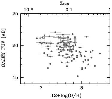
(a)

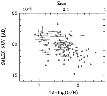
(b)

Figure 11: The distributions of GALEX FUV- (left) and NUV-band (right) photometry for the compiled EMPGs and MPGs as a function of metallicity. The $3\sigma$ upper-limits are adopted on the photometry for the sources without a significant detection.

4 UV Properties of EMPGs

The EMPGs compiled in this study also provide important anchors of properties in the early phase of galaxy evolution that will be useful for high-redshift galaxy studies. In this section, we present the properties of EMPGs in the rest-frame UV wavelength to gain insights into the early star-formation and production of ionizing photons.

4.1 GALEX data

In order to characterize the UV properties of (E)MPGs in the local universe, we utilize the FUV ($\lambda_{\rm eff}\sim 1540$ Å) and NUV ($\lambda_{\rm eff}\sim 2320$ Å) photometric data taken by GALEX (Morrissey et al., 2007). The data are collected from the Mikulski Archive for Space Telescopes (MAST) portal. For each of the objects in our compiled sample (§2.1) we search for the deepest NUV and FUV imaging data that are available at the spatial position of the object. Eight objects are not covered with any pointings of GALEX. For the remaining $177$ objects, we carefully check the downloaded GALEX images to remove sources that are highly contaminated by the neighboring objects due to the low image resolutions (FWHM $\sim 4^{\prime\prime}$ in FUV and $\sim 5^{\prime\prime}$ in NUV). This procedure is particularly important for the nearby stellar clumps/Hii regions where multiple clumps are found in a galaxy, as well as EMPGs that are associated with a bright extended tail (see e.g., Isobe et al. 2020). By comparing with the higher-resolution optical images, we label $62$ objects, all of which are nearby stellar clumps, as blended in the GALEX images. The $70$ ($=8+62$) objects are not used in the analyses of UV properties (but used in the analyses of emission line ratios; §3).

Table 5: GALEX Imaging Surveys

		FUV			NUV
Survey		$N^{o}$	Depth(†)		$N^{o}$	Depth(†)
AIS		$53$	$20.45$		$40$	$21.35$
MIS		$34$	$23.25$		$42$	$23.25$
DIS		$3$	$25.35$		$3$	$24.95$
GII		$17$	$23.4$		$22$	$23.5$
NGS		$8$	$23.6$		$8$	$23.7$

Note. — (${\dagger}$) Limiting magnitude at the $3\sigma$ level. The depths for AIS, MIS, and DIS are given in (Morrissey et al., 2007), and those for GII and NGS are estimated by random aperture photometry.

The GALEX imaging observations from five types of surveys are used for the $115$ objects. These surveys are the All-sky Imaging Survey (AIS), the Medium Imaging Survey (MIS), the Deep Imaging Survey (DIS), the Guest Investigators Survey (GII), and the Nearby Galaxy Survey (NGS). The numbers of sources and the typical depths for each surveys and for each bands are given in Table 5. We use the SExtractor software (Bertin & Arnouts, 1996) to perform source detection and photometry. We identify sources with five adjoining pixels and brightness above $>2\sigma$ of the background, and then cross-match with each of our sources to find a counterpart in the FUV/NUV images within $5^{\prime\prime}$ ($\simeq$ FWHM) from the source position. We adopt MAG_AUTO for the total magnitude if the cross-matched object is brighter than the $3\sigma$ limiting magnitude. We find a high detection rate ($>3\sigma$) in the GALEX images ($103/115$ in FUV and $111/115$ in NUV) for the compiled (E)MPGs. The magnitudes are corrected for Galactic extinction in the same way as detailed in §2.1.2. Figure 11 presents the distributions of GALEX FUV and NUV photometry for our sources ($N^{o}=115$) as a function of metallicity.

In the GALEX FUV and NUV photometric bands, the UV emission lines such as Civ$\lambda 1549$, Heii$\lambda 1640$, and Ciii]$\lambda 1909$ stay and can contribute to the observed GALEX photometry. Nevertheless, the UV emission lines would not have a significant impact on the photometry and the resulting UV properties below. Even the strongest UV emission lines present the maximum EWs as large as $\sim 20$ Å for Ciii] and $\sim 10$ Å for Civ for star-formation dominated systems (Nakajima et al., 2018b). Even with such extreme EWs, the photometry would be boosted by only a negligibly small amount ($\lesssim 0.03$ mag for an average brightness galaxy ($\sim 19.3$ mag) in the sample at $z=0.03$). We therefore do not correct for any possible contribution of the UV emission lines to the observed GALEX photometry.

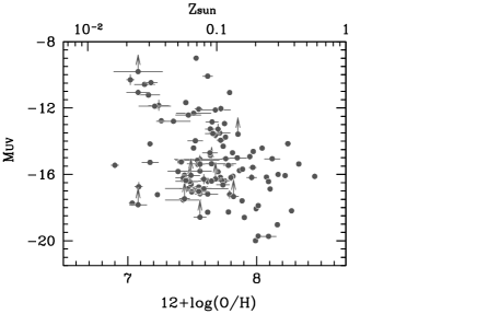
(a)

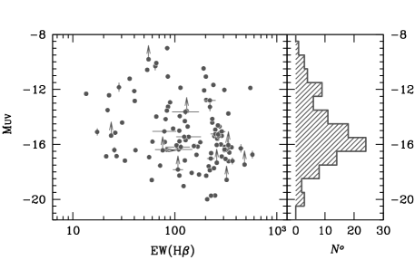
(b)

Figure 12: UV absolute magnitude $M_{\rm UV}$ as a function of metallicity (left) and EW(H$\beta$) (right), and its distribution (at the most right end; the undetected sources are not included in the histogram) for the compiled (E)MPGs in this paper.

4.2 UV absolute magnitude $M_{\rm UV}$

We start with deriving a key fundamental property of UV absolute magnitude, $M_{\rm UV}$ for the compiled metal-poor objects. Here the absolute UV magnitudes are derived from the GALEX FUV band photometry, which probes the rest-frame $\sim 1500$ Å emission, in addition to the luminosity distance. We do not take into account any k-correction for the $M_{\rm UV}$ estimations as the sample is almost built at the similar redshift of $z<0.05$ (Figure 2b). Moreover, the errors in the luminosity distance (or redshift) are not available for the compiled sample, and not included in the $M_{\rm UV}$ calculation. A correction for dust reddening is applied according to the degree of attenuation for nebular emission. We utilize the Balmer decrements and the Calzetti et al. (2000)’s attenuation curve to obtain E(B$-$V) for the nebular emission, divide it by $0.44$ for stellar emission (Calzetti et al., 2000), and correct for the reddening of the FUV stellar light. The corrections are generally small for the metal-poor objects studied in this paper, and our results are not significantly affected by the choice of the attenuation curve and the relationship of E(B$-$V) between stellar and nebular emission. Figure 12 shows the distribution of $M_{\rm UV}$ for the compiled objects as functions of metallicity and EW(H$\beta$). The compiled sample extraordinarily reaches the faintest UV magnitude of $M_{\rm UV}$ $\sim-9$.

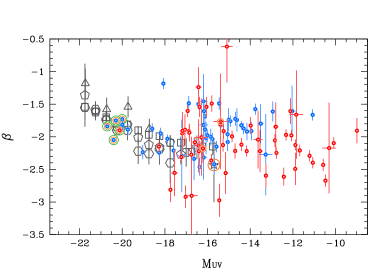
(a)

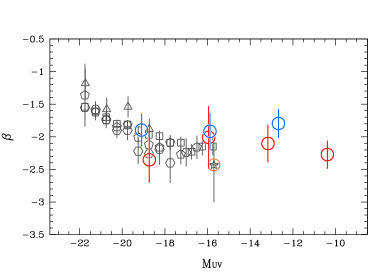
(b)

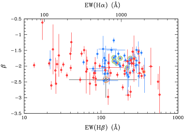
(c)

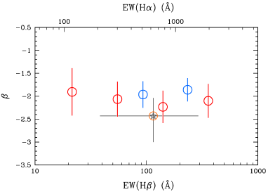
(d)

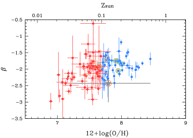
(e)

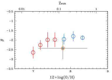
(f)

Figure 13: Relationships of UV slope $\beta$ as a function of $M_{\rm UV}$ (top), EW(H$\beta$) (middle), and metallicity (bottom). In the left panels, our compiled EMPGs (red small circles) and MPGs (blue small circles) are presented on an individual basis, while the binned average relationships for EMPGs (red open circles) and MPGs (blue open circles) are presented with larger symbols in the right panels using the individual data points shown in the left-hand panels. The errorbar represents the standard deviation of each of the binned distribution. The points enclosed with a green circle are $z\simeq 0.3$ green pea galaxies whose $f_{\rm esc}$ is directly measured (Izotov et al., 2016a, b). The other large open symbols denote average relationships at higher-redshifts of $z\sim 2.5$ (triangles), $4$ (squares), $5$ (pentagons), and $6$ (hexagons) (Bouwens et al., 2009, 2014). The open star shows a stacked result of faint LAEs at $z=4-5$ (Maseda et al., 2020). Like the Maseda et al. (2020)’s data-point, the orange-markers represent galaxies whose Ly$\alpha$ is observed to be strong (LAEs with EW(Ly$\alpha$) $>20$ Å; see also Izotov et al. 2020). For high-redshift galaxies whose EW(H$\beta$) is unknown, we substitute EW(H$\alpha$) using the empirical conversion of EW(H$\alpha$)$/$EW(H$\beta$) $=5.47$ (Kojima et al., 2020).

4.3 UV slope $\beta$

Our next interest is to determine the rest-frame UV continuum slope $\beta$ ($f_{\lambda}\propto\lambda^{\beta}$) for EMPGs and examine the distribution of $\beta$ toward the lowest metallicity and faintest UV luminosity. We estimate the UV continuum slope $\beta$ using two wavelength photometric points of GALEX FUV and NUV band. We note again that the k-correction would be negligible in our $\beta$ measurements (§4.2). The wavelength range of $\sim 1500$–$2300$ Å is consistent with those used for $\beta$ measurements in higher-redshift galaxies (e.g., Bouwens et al. 2009, 2012). For each object we fit the FUV and NUV magnitudes with a power-law function at the measured redshift and determine $\beta$. We also repeat the fitting to randomly fluctuated photometry following the errors as Gaussian distributions and obtain the $1\sigma$ uncertainty of $\beta$ which encompasses $68$ percent of $\beta$ values drawn from the procedure.

Figure 13 presents how the UV slopes of (E)MPGs are distributed as a function of absolute UV magnitude, EW(H$\beta$), and metallicity. The left panels show the individual objects, while the right panels present an average value of $\beta$ for a bin of the abscissa quantity, with red symbols for EMPGs and blue for MPGs. The relationship between $\beta$ and $M_{\rm UV}$ (top panels) reveals that EMPGs overall present a small value of $\beta$ from $\sim-1.9$ to $\sim-2.3$ in the range of $M_{\rm UV}$ $=-18$ to $-10$ on average, mostly independent of the UV luminosity. The reference sample of MPGs in the local universe covers a slightly bright but still faint range of $M_{\rm UV}$ $=-20$ to $-12$, showing a similarly flat relationship of $\beta$ as a function of $M_{\rm UV}$ and showing a similarly small value of $\beta$ from $\sim-1.8$ to $\sim-2.0$. The difference between the EMPG and MPG samples is therefore not significant on the $\beta$ vs. $M_{\rm UV}$ plane. At higher-redshifts ($z\gtrsim 3$), using continuum-selected galaxies such as Lyman break galaxies (LBGs), earlier studies have indicated a decreasing trend of $\beta$ toward a fainter $M_{\rm UV}$ on average in the bright end of $M_{\rm UV}$ $=-22$ to $-17$ (e.g., Bouwens et al. 2009, 2014). On the other hand, some studies find a rather flat trend of $\beta\sim-2$ irrespective of $M_{\rm UV}$ (Finkelstein et al., 2012; Dunlop et al., 2013) as similarly seen in the local (E)MPG sample. The relationship between $\beta$ and $M_{\rm UV}$ remains controversial at high-redshift, and will be revisited below.

The middle panels of Figure 13 show the distribution of $\beta$ as a function of EW(H$\beta$). We are interested in EW(H$\beta$) to use it as a proxy for stellar age as it corresponds to the current star-formation activity divided by the stellar mass (i.e., specific star-formation rate; sSFR). We find a very weak trend of decreasing $\beta$ toward a larger EW(H$\beta$) in the EMPG sample. Even the largest EW(H$\beta$) objects ($>200$ Å) present a large scatter of $\beta$. At first sight, it is weird to find such a weak correlation because a dust content is thought to be tightly linked with the past star-formation history and hence the stellar age. We speculate this would be due to the fact that EW(H$\beta$) is a measure of the stellar age based on the current star-formation activity. Past star-formation episodes would play a role in dust production even for the largest EW(H$\beta$) galaxies that are experiencing another phase of active star-formation. Accordingly, EW(H$\beta$) would not be the primary governing the UV continuum slope especially in the local universe.

At the bottom, the relationship between $\beta$ and metallicity is presented. We clearly see a trend such that the UV continuum slope gets smaller at a lower metallicity, particularly at $12+\log({\rm O/H})$ $\lesssim 7.3$. At the lowest metallicity, the $\beta$ value reaches $\beta\sim-2.6$, which is as small as the intrinsic slope $\beta_{0}$ theoretically predicted (Reddy et al., 2018b). This supports that EMPGs, especially with $12+\log({\rm O/H})$ $\simeq 7.0$ or less metallicity, are almost dust-free systems as the productions and abundances of dust and metals are closely related to each other, both following the past star-formation history. A relatively large scatter of metallicity for a given $M_{\rm UV}$ and EW(H$\beta$) (Figures 2a(top) and 12(right)) would weaken the relationship and result in a flat trend of $\beta$ as seen in the top and middle panels. On the other hand, the high-redshift samples are usually continuum-selected and hence magnitude-limited. Following a relatively tight luminosity–metallicity relationship and its redshift evolution (e.g., Zahid et al. 2011), fainter and higher-redshift galaxies tend to be metal-poorer. The negative relationship between $\beta$ and $M_{\rm UV}$ observed in high-redshift UV-selected LBGs and its possible redshift evolution toward smaller $\beta$ as seen in the top panels would thus be caused by such a luminosity–metallicity relation.

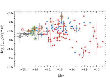
(a)

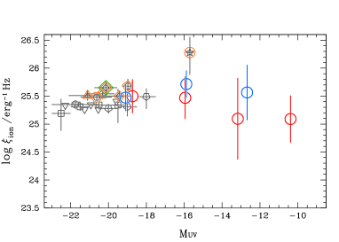
(b)

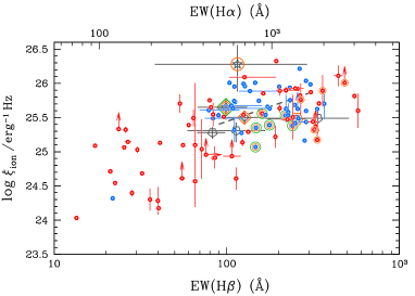
(c)

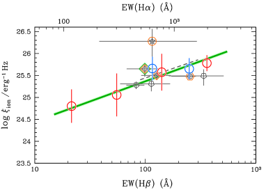
(d)

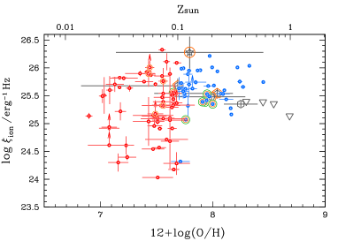
(e)

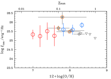
(f)

Figure 14: Same as Figure 13 but for the relationships of ionizing photon production efficiency $\xi_{\rm ion}$. Low-$z$ galaxies are as plotted in Figure 13. The other large open symbols denote average relationships at higher-redshifts; continuum-selected LBGs at $z=1.4-2.6$ (inverted open triangles; Shivaei et al. 2018), at $z=2-4$ ($30$ deg-rotated hexagon; Nakajima et al. 2018b; Le Fèvre et al. 2019), at $z=3.8-5.0$ (open squares; Bouwens et al. 2016), and at $z=4-5$ (inverted open pentagons; Lam et al. 2019). Orange-marked symbols are LAEs at $z=3$ (open pentagons from Nakajima et al. 2018a based on the UV emission lines, open diamonds from Nakajima et al. 2020 based on the H$\beta$ spectroscopy), at $z=4-5$ (star; Maseda et al. 2020, at $z=4.9$ (hexagon; Harikane et al. 2018), and at $z=6-7$ (triangle; Matthee et al. 2017). We note that the $\xi_{\rm ion}$ is corrected for the escaping ionizing photons for the sources with an $f_{\rm esc}$-measurement (green-enclosed;(Izotov et al., 2016a, b; Schaerer et al., 2016; Izotov et al., 2018a; Schaerer et al., 2018; Nakajima et al., 2020)). Two individual galaxies at $z=7-8$ are also presented with magenta circles whose Ly$\alpha$ and UV emission lines are detected (Stark et al., 2015b, 2017). In the middle panels, an average EW(H$\beta$)–$\xi_{\rm ion}$ relationship seen in extreme emission line galaxies at $z=1.3-2.4$ is illustrated with a gray dashed line (Tang et al., 2019). Our best-fit relationship of Equation (3) is presented with a green solid line, confirming the previously known relationship but over a wider range of EW(H$\beta$) of $\sim 10-600$ Å.

4.4 Ionizing photon production efficiency $\xi_{\rm ion}$

Another key UV property is the ionizing photon production efficiency, $\xi_{\rm ion}$. This quantity represents the number of hydrogen-ionizing photons per UV luminosity;

$$\xi_{\rm ion}=\frac{Q_{{\rm H}^{0}}}{L_{\rm UV}}.$$ (2)

where $Q_{{\rm H}^{0}}$ is the ionizing photon production rate below $912$ Å, and $L_{\rm UV}$ is the intrinsic UV continuum luminosity typically at around $1500$ Å. The number of ionizing photons, $Q_{{\rm H}^{0}}$, can be determined via hydrogen recombination lines such as H$\alpha$ and H$\beta$ (e.g Leitherer & Heckman 1995), and the UV luminosity, $L_{\rm UV}$, is now derived from the GALEX FUV band photometry for the nearby galaxies (as $M_{\rm UV}$ estimated; see §4.2). Note that the conversion of $Q_{{\rm H}^{0}}$ assumes no escaping ionizing photons, i.e., all are converted into recombination radiation unless otherwise specified. We will revisit the assumption later.

A crucial step is to match the apertures for the measurements of hydrogen recombination lines and FUV band photometry. This is complicated by the spectroscopic measurements which were taken heterogeneously. We then use the total H$\alpha$ flux estimated from the excess in the broadband photometry, which are measured in a consistent way as the total magnitude of GALEX FUV. As illustrated in Figure 12, our EMPG sample present an intense hydrogen recombination lines of EW(H$\beta$) ($\sim 10$–$600$ Å at the rest-frame, $\sim 130$ Å median). Given the typical EW ratio of EW(H$\alpha$)$/$EW(H$\beta$) $=5.47$ (Kojima et al., 2020), H$\alpha$ EWs are supposed to be very large on average for the EMPGs ($\sim 700$ Å) and boost the photometry of the broadband where the H$\alpha$ is redshifted and falls in. We can estimate the strength of H$\alpha$ by evaluating the excess in the photometric broadband SED. We retrieve the broadband photometric data from the archives of the SDSS Data Release 16 and the HSC-SSP S20A Data Release. We use the HSC $riz$ band photometry for those in the HSC-SSP footprint. Otherwise we use the SDSS $riz$ band photometry. Fifteen sources, most of which are in the MPG sample from Guseva et al. (2007), are not cross-matched with anything on the two catalogs, and thus not used in the following $\xi_{\rm ion}$ analyses. We adopt the photometry of cmodel (HSC) and ModelMag (SDSS) which delivers the total magnitude for each of the broadbands. At $z\lesssim 0.055$ with HSC, the $r$-band captures the H$\alpha$ line, and the $i$- and $z$-bands are used for the continuum estimation. At a higher-redshift (up to the highest redshift of $z=0.13$ in our sample), we use the $i$-band to probe the H$\alpha$ (+continuum) and the $z$-band for the continuum. We use a BPASS SED with a stellar metallicity of $Z\sim 0.07$ $Z_{\odot}$, constant star-formation, and with an age of $50$ Myr to assume the shape of the continuum around $iz$-bands. A different demarcation redshift of $0.040$ is adopted for the SDSS photometry. For each of the objects we use the systemic redshift determined from the optical spectroscopy as well as the actual transmission curves of the broadbands to translate the broadband excess into the flux of H$\alpha$. We ignore the small contributions ($\lesssim 10$ %) of the weaker emission lines such as [N ii]$\lambda 6584$ and [S ii]$\lambda\lambda 6717,6731$ for the EMPG sample. The flux of H$\alpha$ is then reddening-corrected with the E(B$-$V) value estimated from the Balmer decrements of the spectroscopy data with the Calzetti et al. (2000)’s attenuation law. Finally, as a sanity check, we compare the dust-corrected fluxes of H$\alpha$ derived from the above method (i.e., the broadband excess) and spectroscopy. If the spectroscopic measure of H$\alpha$ is not available, we substitute the dust-corrected H$\beta$ multiplied by the intrinsic H$\alpha$$/$H$\beta$ ratio ($2.86$ in the Case B recombination) to be compared with the H$\alpha$ strength from the broadband excess. The difference corresponds to the aperture correction for the slit- or fiber-loss in the spectroscopic observation. The difference typically varies from $1.0$ to $2.2$ ($1.4$ median), which are reasonable as aperture corrections for EMPGs (e.g., Izotov et al. 2011).

Figure 14 provides the distribution of $\xi_{\rm ion}$ as a function of various key properties of $M_{\rm UV}$, EW(H$\beta$), and metallicity. We have now explored the $\xi_{\rm ion}$ for the EMPGs over the wide ranges of properties, down to $M_{\rm UV}$ $\sim-10$, EW(H$\beta$) $\sim 10$–$600$ Å, and $12+\log({\rm O/H})$ down to $\sim 6.9$. At the faint end of the UV luminosity $M_{\rm UV}$ $\gtrsim-15$, a large variation of $\xi_{\rm ion}$ is interestingly recognized especially for the EMPG sample (top panels of Figure 14). This is in contrast to the previous studies at high-redshift where an almost flat, or a weakly increasing trend of $\xi_{\rm ion}$ is suggested with UV luminosity decreasing in the range of $M_{\rm UV}$ from $-22$ to $\sim-19$ (e.g., Bouwens et al. 2016; Shivaei et al. 2018; Nakajima et al. 2018a). A stacking of faint, strong Ly$\alpha$ emitters at $z=4-5$ infers a very large value of $\log$ $\xi_{\rm ion}$ of $26.3$ albeit with a large uncertainty, and supports an elevated ionizing photon production efficiency in faint galaxies (Maseda et al., 2020). LAEs are generally thought to be more efficient producers of ionizing photons at a given UV luminosity compared to continuum-selected LBGs (Trainor et al., 2016; Nakajima et al., 2016; Matthee et al., 2017; Harikane et al., 2018; Nakajima et al., 2018a, 2020). The EMPGs examined in this study do not apparently follow the trend. Although the typical $\xi_{\rm ion}$ matches with those reported in high-redshift galaxies at $M_{\rm UV}$ $\sim-19$, it rather decreases with $M_{\rm UV}$ with a tendency that MPGs have a more or less larger $\xi_{\rm ion}$ value than EMPGs for a given UV luminosity. The bottom panels of Figure 14 clarify the metallicity dependence of $\xi_{\rm ion}$. A large variation remains at the lowest metallicity of $12+\log({\rm O/H})$ $\sim 7.0$ whose $\xi_{\rm ion}$ varies from $log$ $\xi_{\rm ion}$ $\sim 24.0$ to $26.0$. Faint UV luminosity and/or low metallicity in gas-phase would not be the primary properties that govern the efficient production of ionizing photons. We will turn back to these puzzling trends later.

On the other hand, the middle panels of Figure 14 illustrate that EW(H$\beta$) is well-correlated with $\xi_{\rm ion}$ in a positive manner with a relatively small uncertainty. Both the EMPG and the MPG samples fall on the same relationship, with the following equation form:

$$\log\xi_{\rm ion}=23.53+0.92\times\log{\rm EW}({\rm H}\beta).$$ (3)

Such a tight correlation has been suggested in earlier studies in the local universe (Chevallard et al., 2018), at $z\sim 1-2$ (Tang et al., 2019), at $z\sim 3$ (Nakajima et al., 2020), and even at $z\sim 4-5$ (Harikane et al., 2018; Lam et al., 2019). This work confirms the same relationship for metal-poor galaxies, and also suggests it holds over the wider range of EW(H$\beta$) than previously explored, down to $\sim 10$ Å and up to $\sim 600$ Å. The stacked faint LAEs at $z\sim 4-5$ interestingly appears to fall above the relationship (Maseda et al., 2020), although the large uncertainty remains both in $\xi_{\rm ion}$ and EW(H$\alpha$). Following the apparently universal trend as a function of EWs of Hydrogen Balmer lines, the production efficiency of ionizing photons would be mainly governed by the stellar age of the current star-formation. This is reasonable as it probes the relative abundance of the youngest, most massive stars (age of $\lesssim 10$ Myr) to that of less massive, long-lived stars that can contribute to the non-ionizing UV radiation (age of $\lesssim 100$ Myr). Theoretically a metal-poorer stellar population would present a harder ionizing spectrum due to several effects such as metal blanketing, rotational hardening, and binary evolution (e.g. Levesque et al. 2012; Kewley et al. 2013; Eldridge et al. 2017). In the current sample, however, we do not see any significant secondary dependence of metallicity on the relationship, albeit with a caveat that the metallicity we refer to is the gas-phase oxygen abundance while the stellar metallicity, especially the iron abundance, controls the hardness of ionizing spectrum (e.g., Steidel et al. 2016; Cullen et al. 2019). We need such metal absorption studies for EMPGs to discuss the stellar metallicity dependences. The lack of metallicity dependence on $\xi_{\rm ion}$ in our sample can be partly because we explore only the lowest metallicity range below the sub-solar value. Indeed, a weak-but-decreasing trend of $\xi_{\rm ion}$ with metallicity is seen in the $z=2-3$ sample on average in the high metallicity range of $12+\log({\rm O/H})$ $>8.2$ (Shivaei et al., 2018), although this may be a result of the correlation between EW(H$\beta$) and metallicity in the MOSDEF sample (Reddy et al., 2018a). Moreover, the assumption of zero escape fraction may not be realistic for extremely faint, metal-poor systems (see below).

We now revisit the puzzling trends found in the $M_{\rm UV}$ vs. $\xi_{\rm ion}$ plot following the strong dependence of $\xi_{\rm ion}$ on EW(H$\beta$). At the bright end of Figure 14, the relatively large $\xi_{\rm ion}$ values reported on average in high-redshift galaxies are primarily due to a large EW in galaxies typically found at high-redshift (Khostovan et al., 2016; Faisst et al., 2016; Reddy et al., 2018a). Among these high-redshift galaxies, less massive galaxies with a fainter $M_{\rm UV}$ tend to be younger and present a larger EW, and hence have a harder $\xi_{\rm ion}$ to set up the weakly increasing trend. In particular, LAEs with a stronger EW(Ly$\alpha$) show a larger EW(H$\beta$), and are associated with a harder ionizing spectrum as marked with orange symbols in Figure 14. (Nakajima et al., 2016; Matthee et al., 2017; Harikane et al., 2018; Nakajima et al., 2018a, 2020; Maseda et al., 2020). At the fainter end of $M_{\rm UV}$ ($\gtrsim 15$) in the current plot, half of the EMPGs in the faint $M_{\rm UV}$ range have a low value of EW(H$\beta$) below $\sim 80$ Å (Figure 12) and thus lower the typical value of $\xi_{\rm ion}$ in the current compilation. The MPGs, which are compiled in a less complete manner (§2.1.3) show a biased distribution of EW(H$\beta$) toward larger values (Figure 2a) and thus tend to have a larger $\xi_{\rm ion}$ than the EMPGs for a given $M_{\rm UV}$.

Finally, we note again that the current $\xi_{\rm ion}$ measurements for the compiled galaxies assume no escaping ionizing photons. In Figure 14, we plot the intrinsic $\xi_{\rm ion}$ values only for some green pea galaxies at $z\simeq 0.3$ and LAEs at $z\simeq 3$ whose escape fraction of ionizing photons, $f_{\rm esc}$, is directly measured ($f_{\rm esc}$ $\sim 0.05$ to $\sim 0.5$; Izotov et al. 2016a, b; Schaerer et al. 2016; Izotov et al. 2018a; Schaerer et al. 2018; Fletcher et al. 2019; Nakajima et al. 2020). The intrinsic values are greater than the observed ones by a factor of $1/(1-f_{\rm esc})$, which ranges from $\sim 1.05$ to as large as $2$ in the above cases. In this sense, the $\xi_{\rm ion}$ values currently estimated for the remaining (E)MPGs serve as lower-limits, to be precise. This could be part of another reason why the $\xi_{\rm ion}$ of the (E)MPGs appear not so large at the extremely faint and low-metallicity regimes. Indeed, galaxies with a bluer UV continuum slope, as blue as the intrinsic slope $\beta_{0}$, tend to be more associated with a LyC leakage (e.g., Zackrisson et al. 2013, 2017). Following the trend between $\beta$ and metallicity (bottom panels in Figure 13), EMPGs are thought to have a higher chance to present a non-zero $f_{\rm esc}$. On the other hand, the $f_{\rm esc}$ uncertainty would not break the relationship between $\xi_{\rm ion}$ and EW(H$\beta$) because EW(H$\beta$) is observed to become small by the same factor of $1/(1-f_{\rm esc})$ as $\xi_{\rm ion}$ (see also the slope of Equation (3) is almost unity). Although direct LyC observations for the local (E)MPGs are challenging because they are too near-by ($z\lesssim 0.05$) to be observed with HST/COS in the wavelength below the Lyman limit, indirect methods such as using the Ly$\alpha$’s spectral profile and the flux at the systemic velocity (e.g., Verhamme et al. 2017; Vanzella et al. 2019; Naidu et al. 2021) could help understand the local (E)MPGs’ intrinsic nature of ionizing photon production/escape and its dependence on the galaxy’s properties.

5 Summary

We investigate the optical-line metallicity indicators together with the fundamental ultra-violet (UV) properties of low-mass, extremely metal-poor galaxies (EMPGs) to provide useful anchors for forthcoming spectroscopic studies in the early universe. We make use of the EMPRESS sample (Kojima et al., 2020) and perform a follow-up spectroscopic observation to enlarge the EMPG sample. Compiling previously known metal-poor galaxies from the literature, we build a large sample of EMPGs ($N^{o}=103$) covering a large parameter space of magnitude ($M_{i}$ from $-19$ to $-7$ and $M_{\rm UV}$ from $-20$ to $-9$) and H$\beta$ equivalent width (EW(H$\beta$) from $10$ to $600$ Å), i.e., wide ranges of stellar mass and star-formation rate. Our main results regarding the metallicity indicators are summarized as follows.

1. Utilizing the largest EMPG sample as well as the stacked spectra of $120,000$ SDSS galaxies (Curti et al., 2017, 2020), we derive the relationships between strong optical line ratios and gas-phase metallicity over the range of $12+\log({\rm O/H})$ $=6.9$ to $8.9$ corresponding to $0.02$ to $2$ solar metallicity $Z_{\odot}$ fully based on the reliable metallicity measurements of the direct $T_{e}$ method.

2. We confirm that R23-index, ([O iii]+[O ii])/H$\beta$, shows the smallest scatter in the relation with the metallicity measurements ($\Delta$ log (O/H) $=0.14$) over the full metallicity range, suggesting that R23-index is most reliable among various metallicity indicators over the wide range of metallicity. Unlike R23-index, the other metallicity indicators do not use a sum of singly and doubly ionized lines and cannot trace both low and high ionization gas. A caveat is an R23-based metallicity becomes less accurate around $12+\log({\rm O/H})$ $\sim 8.0\pm 0.2$ as compared to the lower and higher metallicity ranges due to the two-branch nature.

3. We find that the accuracy of the metallicity indicators, including the famous ones such as R3-index and N2-index, becomes significantly improved (by a factor of as large as 2), if one uses H$\beta$ equivalent width measurements that tightly correlate with ISM ionization states. This application is supported by our CLOUDY photoionization modeling, and suggested to work irrespective of redshift. We argue that it is crucial to correct for the ISM ionization condition in estimating the metallicity if the strong line methods, especially when using only low- or high-ionization lines are used. Such a correction would be of particular importance when discussing the mass-metallicity relation, its dependence on star-formation activity, and its cosmic evolution.

Moreover, the analysis of GALEX FUV and NUV band photometry for the EMPGs allows us to characterize the UV properties of UV absolute magnitude $M_{\rm UV}$, UV continuum slope $\beta$, and ionizing photon production efficiency $\xi_{\rm ion}$ for the extreme population of EMPGs. The main findings are as follows.

1. We identify the UV slope $\beta$ is best-correlated with metallicity below 12+log(O/H) $\lesssim 7.4$. The most metal-deficient galaxies with $12+\log({\rm O/H})$ $\sim 7$ on average show the lowest $\beta$ value almost close to the intrinsic UV continuum slope $\beta_{0}=-2.6$. The negative correlation between $\beta$ and $M_{\rm UV}$ known in high-redshift UV-selected galaxies would be caused by a luminosity–metallicity relation.

2. We confirm the ionizing photon production efficiency $\xi_{\rm ion}$ is best-correlated with EWs of Hydrogen Balmer lines of H$\alpha$ and H$\beta$ over a wide range from EW(H$\beta$) $=10$ Å to $600$ Å. A large variation of $\xi_{\rm ion}$ is recognized even for galaxies with the faintest UV luminosity ($M_{\rm UV}$ $\gtrsim-15$) and the lowest metallicity ($12+\log({\rm O/H})$ $\lesssim 7.69$). The variations of $\xi_{\rm ion}$ as well as EW(H$\beta$) for a given metallicity worsen the accuracy of the metallicity diagnostics as discussed above.

The metallicity-sensitive emission line ratios and the UV properties for the compiled 103 EMPGs are publicly available in the form of ASCII table as partly listed in Table 6.

Table 6: Properties of Compiled 103 EMPGs

ID	REDSHIFT	12+LOG(O/H)	e_12+LOG(O/H)	EW(H-beta)	Mi	Muv	BETA	LOG(XIION)	R23-INDEX	e_R23-INDEX	R2-INDEX	e_R2-INDEX	R3-INDEX	e_R3-INDEX	O32-INDEX	e_O32-INDEX	N2-INDEX	e_N2-INDEX	O3N2-INDEX	e_O3N2-INDEX	S2-INDEX	e_S2-INDEX	Ne3O2-INDEX	e_Ne3O2-INDEX
–	–	–	–	0.1nm	mag	mag	–	[Hz.J-1.10+7]	–	–	–	–	–	–	–	–	–	–	–	–	–	–	–	–
J0036+0052	0.0282	7.390	0.080	79.7	-16.21	-15.82	-2.36	25.75		0.005	-0.124	0.011	0.605	0.006	0.729	0.011	-2.121		2.726	0.039	-1.390	0.015	-0.381	0.016
J01074656+01035206	0.0020	7.679	0.118	40.0	-9.80	-12.12	-1.61	24.28		0.016	0.432	0.019	0.293	0.018	-0.139	0.017							-1.180	0.073
J0113+0052No.1	0.0038	7.150	0.090	40.7	-10.22					0.022	-0.083	0.040	0.275	0.022	0.358	0.038	$<$-2.133				$<$-1.656		-0.541	0.067
J0113+0052No.2	0.0038	7.320	0.040	20.8	-10.20					0.029	0.298	0.035	-0.002	0.030	-0.300	0.034	-1.539		1.537	0.064	-0.878	0.031	$<$-1.466
J0113+0052No.3	0.0038	7.300	0.080	30.0	-10.23					0.024	0.184	0.035	0.312	0.026	0.127	0.032	$<$-2.128				-1.063	0.032	$<$-1.352

Note. — Table 6 is published in its entirety in the machine-readable format. A portion is shown here for guidance regarding its form and content.

References

- Aihara et al. (2018) Aihara, H., Arimoto, N., Armstrong, R., et al. 2018, PASJ, 70, S4, doi: 10.1093/pasj/psx066
- Andrews & Martini (2013) Andrews, B. H., & Martini, P. 2013, ApJ, 765, 140, doi: 10.1088/0004-637X/765/2/140
- Asplund et al. (2009) Asplund, M., Grevesse, N., Sauval, A. J., & Scott, P. 2009, ARA&A, 47, 481, doi: 10.1146/annurev.astro.46.060407.145222
- Berg et al. (2018) Berg, D. A., Erb, D. K., Auger, M. W., Pettini, M., & Brammer, G. B. 2018, ApJ, 859, 164, doi: 10.3847/1538-4357/aab7fa
- Berg et al. (2016) Berg, D. A., Skillman, E. D., Henry, R. B. C., Erb, D. K., & Carigi, L. 2016, ApJ, 827, 126, doi: 10.3847/0004-637X/827/2/126
- Berg et al. (2022) Berg, D. A., James, B. L., King, T., et al. 2022, arXiv e-prints, arXiv:2203.07357. https://arxiv.org/abs/2203.07357
- Bertin & Arnouts (1996) Bertin, E., & Arnouts, S. 1996, A&AS, 117, 393, doi: 10.1051/aas:1996164
- Bian et al. (2018) Bian, F., Kewley, L. J., & Dopita, M. A. 2018, ApJ, 859, 175, doi: 10.3847/1538-4357/aabd74
- Blanc et al. (2015) Blanc, G. A., Kewley, L., Vogt, F. P. A., & Dopita, M. A. 2015, ApJ, 798, 99, doi: 10.1088/0004-637X/798/2/99
- Bouwens et al. (2016) Bouwens, R. J., Smit, R., Labbé, I., et al. 2016, ApJ, 831, 176, doi: 10.3847/0004-637X/831/2/176
- Bouwens et al. (2009) Bouwens, R. J., Illingworth, G. D., Franx, M., et al. 2009, ApJ, 705, 936, doi: 10.1088/0004-637X/705/1/936
- Bouwens et al. (2012) Bouwens, R. J., Illingworth, G. D., Oesch, P. A., et al. 2012, ApJ, 754, 83, doi: 10.1088/0004-637X/754/2/83
- Bouwens et al. (2014) —. 2014, ApJ, 793, 115, doi: 10.1088/0004-637X/793/2/115
- Brown et al. (2016) Brown, J. S., Martini, P., & Andrews, B. H. 2016, MNRAS, 458, 1529, doi: 10.1093/mnras/stw392
- Byler et al. (2018) Byler, N., Dalcanton, J. J., Conroy, C., et al. 2018, ApJ, 863, 14, doi: 10.3847/1538-4357/aacd50
- Calzetti et al. (2000) Calzetti, D., Armus, L., Bohlin, R. C., et al. 2000, ApJ, 533, 682, doi: 10.1086/308692
- Cardamone et al. (2009) Cardamone, C., Schawinski, K., Sarzi, M., et al. 2009, MNRAS, 399, 1191, doi: 10.1111/j.1365-2966.2009.15383.x
- Cardelli et al. (1989) Cardelli, J. A., Clayton, G. C., & Mathis, J. S. 1989, ApJ, 345, 245, doi: 10.1086/167900
- Chabrier (2003) Chabrier, G. 2003, PASP, 115, 763, doi: 10.1086/376392
- Chevallard et al. (2018) Chevallard, J., Charlot, S., Senchyna, P., et al. 2018, MNRAS, 479, 3264, doi: 10.1093/mnras/sty1461
- Chisholm et al. (2018) Chisholm, J., Gazagnes, S., Schaerer, D., et al. 2018, A&A, 616, A30, doi: 10.1051/0004-6361/201832758
- Christensen et al. (2012) Christensen, L., Laursen, P., Richard, J., et al. 2012, MNRAS, 427, 1973, doi: 10.1111/j.1365-2966.2012.22007.x
- Cirasuolo et al. (2014) Cirasuolo, M., Afonso, J., Carollo, M., et al. 2014, in Society of Photo-Optical Instrumentation Engineers (SPIE) Conference Series, Vol. 9147, Ground-based and Airborne Instrumentation for Astronomy V, ed. S. K. Ramsay, I. S. McLean, & H. Takami, 91470N, doi: 10.1117/12.2056012
- Cowie et al. (2016) Cowie, L. L., Barger, A. J., & Songaila, A. 2016, ApJ, 817, 57, doi: 10.3847/0004-637X/817/1/57
- Cullen et al. (2019) Cullen, F., McLure, R. J., Dunlop, J. S., et al. 2019, MNRAS, 487, 2038, doi: 10.1093/mnras/stz1402
- Curti et al. (2017) Curti, M., Cresci, G., Mannucci, F., et al. 2017, MNRAS, 465, 1384, doi: 10.1093/mnras/stw2766
- Curti et al. (2020) Curti, M., Mannucci, F., Cresci, G., & Maiolino, R. 2020, MNRAS, 491, 944, doi: 10.1093/mnras/stz2910
- Dunlop et al. (2013) Dunlop, J. S., Rogers, A. B., McLure, R. J., et al. 2013, MNRAS, 432, 3520, doi: 10.1093/mnras/stt702
- Edmunds & Pagel (1984) Edmunds, M. G., & Pagel, B. E. J. 1984, MNRAS, 211, 507, doi: 10.1093/mnras/211.3.507
- Eldridge et al. (2017) Eldridge, J. J., Stanway, E. R., Xiao, L., et al. 2017, PASA, 34, e058, doi: 10.1017/pasa.2017.51
- Erb et al. (2010) Erb, D. K., Pettini, M., Shapley, A. E., et al. 2010, ApJ, 719, 1168, doi: 10.1088/0004-637X/719/2/1168
- Faisst (2016) Faisst, A. L. 2016, ApJ, 829, 99, doi: 10.3847/0004-637X/829/2/99
- Faisst et al. (2016) Faisst, A. L., Capak, P., Hsieh, B. C., et al. 2016, ApJ, 821, 122, doi: 10.3847/0004-637X/821/2/122
- Feltre et al. (2016) Feltre, A., Charlot, S., & Gutkin, J. 2016, MNRAS, 456, 3354, doi: 10.1093/mnras/stv2794
- Finkelstein et al. (2012) Finkelstein, S. L., Papovich, C., Salmon, B., et al. 2012, ApJ, 756, 164, doi: 10.1088/0004-637X/756/2/164
- Fletcher et al. (2019) Fletcher, T. J., Tang, M., Robertson, B. E., et al. 2019, ApJ, 878, 87, doi: 10.3847/1538-4357/ab2045
- Flury et al. (2022) Flury, S. R., Jaskot, A. E., Ferguson, H. C., et al. 2022, arXiv e-prints, arXiv:2201.11716. https://arxiv.org/abs/2201.11716
- Guseva et al. (2007) Guseva, N. G., Izotov, Y. I., Papaderos, P., & Fricke, K. J. 2007, A&A, 464, 885, doi: 10.1051/0004-6361:20066067
- Gutkin et al. (2016) Gutkin, J., Charlot, S., & Bruzual, G. 2016, MNRAS, 462, 1757, doi: 10.1093/mnras/stw1716
- Harikane et al. (2018) Harikane, Y., Ouchi, M., Shibuya, T., et al. 2018, ApJ, 859, 84, doi: 10.3847/1538-4357/aabd80
- Henry et al. (2015) Henry, A., Scarlata, C., Martin, C. L., & Erb, D. 2015, ApJ, 809, 19, doi: 10.1088/0004-637X/809/1/19
- Hirschauer et al. (2016) Hirschauer, A. S., Salzer, J. J., Skillman, E. D., et al. 2016, ApJ, 822, 108, doi: 10.3847/0004-637X/822/2/108
- Hirschmann et al. (2019) Hirschmann, M., Charlot, S., Feltre, A., et al. 2019, MNRAS, 487, 333, doi: 10.1093/mnras/stz1256
- Hsyu et al. (2017) Hsyu, T., Cooke, R. J., Prochaska, J. X., & Bolte, M. 2017, ApJ, 845, L22, doi: 10.3847/2041-8213/aa821f
- Hutchison et al. (2019) Hutchison, T. A., Papovich, C., Finkelstein, S. L., et al. 2019, ApJ, 879, 70, doi: 10.3847/1538-4357/ab22a2
- Isobe et al. (2020) Isobe, Y., Ouchi, M., Kojima, T., et al. 2020, arXiv e-prints, arXiv:2004.11444. https://arxiv.org/abs/2004.11444
- Isobe et al. (2021) Isobe, Y., Ouchi, M., Suzuki, A., et al. 2021, arXiv e-prints, arXiv:2108.03850. https://arxiv.org/abs/2108.03850
- Izotov et al. (2019a) Izotov, Y. I., Guseva, N. G., Fricke, K. J., & Henkel, C. 2019a, A&A, 623, A40, doi: 10.1051/0004-6361/201834768
- Izotov et al. (2009) Izotov, Y. I., Guseva, N. G., Fricke, K. J., & Papaderos, P. 2009, A&A, 503, 61, doi: 10.1051/0004-6361/200911965
- Izotov et al. (2011) Izotov, Y. I., Guseva, N. G., & Thuan, T. X. 2011, ApJ, 728, 161, doi: 10.1088/0004-637X/728/2/161
- Izotov et al. (2016a) Izotov, Y. I., Orlitová, I., Schaerer, D., et al. 2016a, Nature, 529, 178, doi: 10.1038/nature16456
- Izotov et al. (2006a) Izotov, Y. I., Papaderos, P., Guseva, N. G., Fricke, K. J., & Thuan, T. X. 2006a, A&A, 454, 137, doi: 10.1051/0004-6361:20065100
- Izotov et al. (2016b) Izotov, Y. I., Schaerer, D., Thuan, T. X., et al. 2016b, MNRAS, 461, 3683, doi: 10.1093/mnras/stw1205
- Izotov et al. (2018a) Izotov, Y. I., Schaerer, D., Worseck, G., et al. 2018a, MNRAS, 474, 4514, doi: 10.1093/mnras/stx3115
- Izotov et al. (2020) —. 2020, MNRAS, 491, 468, doi: 10.1093/mnras/stz3041
- Izotov et al. (2006b) Izotov, Y. I., Stasińska, G., Meynet, G., Guseva, N. G., & Thuan, T. X. 2006b, A&A, 448, 955, doi: 10.1051/0004-6361:20053763
- Izotov & Thuan (2007) Izotov, Y. I., & Thuan, T. X. 2007, ApJ, 665, 1115, doi: 10.1086/519922
- Izotov et al. (2012a) Izotov, Y. I., Thuan, T. X., & Guseva, N. G. 2012a, A&A, 546, A122, doi: 10.1051/0004-6361/201219733
- Izotov et al. (2019b) —. 2019b, MNRAS, 483, 5491, doi: 10.1093/mnras/sty3472
- Izotov et al. (2021) —. 2021, MNRAS, 504, 3996, doi: 10.1093/mnras/stab1099
- Izotov et al. (2018b) Izotov, Y. I., Thuan, T. X., Guseva, N. G., & Liss, S. E. 2018b, MNRAS, 473, 1956, doi: 10.1093/mnras/stx2478
- Izotov et al. (2012b) Izotov, Y. I., Thuan, T. X., & Privon, G. 2012b, MNRAS, 427, 1229, doi: 10.1111/j.1365-2966.2012.22051.x
- Izotov et al. (2018c) Izotov, Y. I., Worseck, G., Schaerer, D., et al. 2018c, MNRAS, 478, 4851, doi: 10.1093/mnras/sty1378
- Jaskot et al. (2019) Jaskot, A. E., Dowd, T., Oey, M. S., Scarlata, C., & McKinney, J. 2019, arXiv e-prints, arXiv:1908.09763. https://arxiv.org/abs/1908.09763
- Jaskot & Ravindranath (2016) Jaskot, A. E., & Ravindranath, S. 2016, ApJ, 833, 136, doi: 10.3847/1538-4357/833/2/136
- Jiang et al. (2021) Jiang, L., Kashikawa, N., Wang, S., et al. 2021, Nature Astronomy, 5, 256, doi: 10.1038/s41550-020-01275-y
- Kauffmann et al. (2003) Kauffmann, G., Heckman, T. M., Tremonti, C., et al. 2003, MNRAS, 346, 1055, doi: 10.1111/j.1365-2966.2003.07154.x
- Kennicutt (1998) Kennicutt, Robert C., J. 1998, ARA&A, 36, 189, doi: 10.1146/annurev.astro.36.1.189
- Kewley & Dopita (2002) Kewley, L. J., & Dopita, M. A. 2002, ApJS, 142, 35, doi: 10.1086/341326
- Kewley et al. (2013) Kewley, L. J., Dopita, M. A., Leitherer, C., et al. 2013, ApJ, 774, 100, doi: 10.1088/0004-637X/774/2/100
- Khostovan et al. (2016) Khostovan, A. A., Sobral, D., Mobasher, B., et al. 2016, MNRAS, 463, 2363, doi: 10.1093/mnras/stw2174
- Kniazev et al. (2003) Kniazev, A. Y., Grebel, E. K., Hao, L., et al. 2003, ApJ, 593, L73, doi: 10.1086/378259
- Kojima et al. (2020) Kojima, T., Ouchi, M., Rauch, M., et al. 2020, ApJ, 898, 142, doi: 10.3847/1538-4357/aba047
- Kojima et al. (2021) —. 2021, ApJ, 913, 22, doi: 10.3847/1538-4357/abec3d
- Lam et al. (2019) Lam, D., Bouwens, R. J., Labbé, I., et al. 2019, A&A, 627, A164, doi: 10.1051/0004-6361/201935227
- Laporte et al. (2017) Laporte, N., Nakajima, K., Ellis, R. S., et al. 2017, ApJ, 851, 40, doi: 10.3847/1538-4357/aa96a8
- Lara-López et al. (2010) Lara-López, M. A., Cepa, J., Bongiovanni, A., et al. 2010, A&A, 521, L53, doi: 10.1051/0004-6361/201014803
- Le Fèvre et al. (2019) Le Fèvre, O., Lemaux, B. C., Nakajima, K., et al. 2019, A&A, 625, A51, doi: 10.1051/0004-6361/201732197
- Leitherer & Heckman (1995) Leitherer, C., & Heckman, T. M. 1995, ApJS, 96, 9, doi: 10.1086/192112
- Levesque et al. (2012) Levesque, E. M., Leitherer, C., Ekstrom, S., Meynet, G., & Schaerer, D. 2012, ApJ, 751, 67, doi: 10.1088/0004-637X/751/1/67
- Luridiana et al. (2015) Luridiana, V., Morisset, C., & Shaw, R. A. 2015, A&A, 573, A42, doi: 10.1051/0004-6361/201323152
- Mainali et al. (2018) Mainali, R., Zitrin, A., Stark, D. P., et al. 2018, MNRAS, 479, 1180, doi: 10.1093/mnras/sty1640
- Maiolino & Mannucci (2019) Maiolino, R., & Mannucci, F. 2019, A&A Rev., 27, 3, doi: 10.1007/s00159-018-0112-2
- Maiolino et al. (2008) Maiolino, R., Nagao, T., Grazian, A., et al. 2008, A&A, 488, 463, doi: 10.1051/0004-6361:200809678
- Mannucci et al. (2010) Mannucci, F., Cresci, G., Maiolino, R., Marconi, A., & Gnerucci, A. 2010, MNRAS, 408, 2115, doi: 10.1111/j.1365-2966.2010.17291.x
- Marino et al. (2013) Marino, R. A., Rosales-Ortega, F. F., Sánchez, S. F., et al. 2013, A&A, 559, A114, doi: 10.1051/0004-6361/201321956
- Maseda et al. (2020) Maseda, M. V., Bacon, R., Lam, D., et al. 2020, MNRAS, 493, 5120, doi: 10.1093/mnras/staa622
- Matthee et al. (2017) Matthee, J., Sobral, D., Best, P., et al. 2017, MNRAS, 465, 3637, doi: 10.1093/mnras/stw2973
- McGaugh (1991) McGaugh, S. S. 1991, ApJ, 380, 140, doi: 10.1086/170569
- Morrissey et al. (2007) Morrissey, P., Conrow, T., Barlow, T. A., et al. 2007, ApJS, 173, 682, doi: 10.1086/520512
- Nagao et al. (2006) Nagao, T., Maiolino, R., & Marconi, A. 2006, A&A, 459, 85, doi: 10.1051/0004-6361:20065216
- Naidu et al. (2021) Naidu, R. P., Matthee, J., Oesch, P. A., et al. 2021, arXiv e-prints, arXiv:2110.11961. https://arxiv.org/abs/2110.11961
- Nakajima et al. (2016) Nakajima, K., Ellis, R. S., Iwata, I., et al. 2016, ApJ, 831, L9, doi: 10.3847/2041-8205/831/1/L9
- Nakajima et al. (2020) Nakajima, K., Ellis, R. S., Robertson, B. E., Tang, M., & Stark, D. P. 2020, ApJ, 889, 161, doi: 10.3847/1538-4357/ab6604
- Nakajima et al. (2018a) Nakajima, K., Fletcher, T., Ellis, R. S., Robertson, B. E., & Iwata, I. 2018a, MNRAS, 477, 2098, doi: 10.1093/mnras/sty750
- Nakajima & Ouchi (2014) Nakajima, K., & Ouchi, M. 2014, MNRAS, 442, 900, doi: 10.1093/mnras/stu902
- Nakajima et al. (2018b) Nakajima, K., Schaerer, D., Le Fèvre, O., et al. 2018b, A&A, 612, A94, doi: 10.1051/0004-6361/201731935
- Oey et al. (2007) Oey, M. S., Meurer, G. R., Yelda, S., et al. 2007, ApJ, 661, 801, doi: 10.1086/517867
- Oke & Gunn (1983) Oke, J. B., & Gunn, J. E. 1983, ApJ, 266, 713, doi: 10.1086/160817
- Pagel et al. (1979) Pagel, B. E. J., Edmunds, M. G., Blackwell, D. E., Chun, M. S., & Smith, G. 1979, MNRAS, 189, 95, doi: 10.1093/mnras/189.1.95
- Pettini & Pagel (2004) Pettini, M., & Pagel, B. E. J. 2004, MNRAS, 348, L59, doi: 10.1111/j.1365-2966.2004.07591.x
- Pilyugin & Grebel (2016) Pilyugin, L. S., & Grebel, E. K. 2016, MNRAS, 457, 3678, doi: 10.1093/mnras/stw238
- Pilyugin & Thuan (2005) Pilyugin, L. S., & Thuan, T. X. 2005, ApJ, 631, 231, doi: 10.1086/432408
- Plat et al. (2019) Plat, A., Charlot, S., Bruzual, G., et al. 2019, MNRAS, 490, 978, doi: 10.1093/mnras/stz2616
- Pustilnik et al. (2005) Pustilnik, S. A., Kniazev, A. Y., & Pramskij, A. G. 2005, A&A, 443, 91, doi: 10.1051/0004-6361:20053102
- Pustilnik et al. (2010) Pustilnik, S. A., Tepliakova, A. L., Kniazev, A. Y., Martin, J. M., & Burenkov, A. N. 2010, MNRAS, 401, 333, doi: 10.1111/j.1365-2966.2009.15637.x
- Ramambason et al. (2020) Ramambason, L., Schaerer, D., Stasińska, G., et al. 2020, A&A, 644, A21, doi: 10.1051/0004-6361/202038634
- Reddy et al. (2018a) Reddy, N. A., Shapley, A. E., Sanders, R. L., et al. 2018a, ApJ, 869, 92, doi: 10.3847/1538-4357/aaed1e
- Reddy et al. (2018b) Reddy, N. A., Oesch, P. A., Bouwens, R. J., et al. 2018b, ApJ, 853, 56, doi: 10.3847/1538-4357/aaa3e7
- Sánchez Almeida et al. (2016) Sánchez Almeida, J., Pérez-Montero, E., Morales-Luis, A. B., et al. 2016, ApJ, 819, 110, doi: 10.3847/0004-637X/819/2/110
- Sanders et al. (2017) Sanders, R. L., Shapley, A. E., Zhang, K., & Yan, R. 2017, ApJ, 850, 136, doi: 10.3847/1538-4357/aa93e4
- Sanders et al. (2016) Sanders, R. L., Shapley, A. E., Kriek, M., et al. 2016, ApJ, 816, 23, doi: 10.3847/0004-637X/816/1/23
- Sanders et al. (2020) Sanders, R. L., Shapley, A. E., Reddy, N. A., et al. 2020, MNRAS, 491, 1427, doi: 10.1093/mnras/stz3032
- Schaerer et al. (2018) Schaerer, D., Izotov, Y. I., Nakajima, K., et al. 2018, A&A, 616, L14, doi: 10.1051/0004-6361/201833823
- Schaerer et al. (2016) Schaerer, D., Izotov, Y. I., Verhamme, A., et al. 2016, A&A, 591, L8, doi: 10.1051/0004-6361/201628943
- Schlafly & Finkbeiner (2011) Schlafly, E. F., & Finkbeiner, D. P. 2011, ApJ, 737, 103, doi: 10.1088/0004-637X/737/2/103
- Senchyna & Stark (2019) Senchyna, P., & Stark, D. P. 2019, MNRAS, 484, 1270, doi: 10.1093/mnras/stz058
- Senchyna et al. (2019) Senchyna, P., Stark, D. P., Chevallard, J., et al. 2019, MNRAS, 488, 3492, doi: 10.1093/mnras/stz1907
- Senchyna et al. (2017) Senchyna, P., Stark, D. P., Vidal-García, A., et al. 2017, MNRAS, 472, 2608, doi: 10.1093/mnras/stx2059
- Shapley et al. (2015) Shapley, A. E., Reddy, N. A., Kriek, M., et al. 2015, ApJ, 801, 88, doi: 10.1088/0004-637X/801/2/88
- Shivaei et al. (2018) Shivaei, I., Reddy, N. A., Siana, B., et al. 2018, ApJ, 855, 42, doi: 10.3847/1538-4357/aaad62
- Skillman et al. (2013) Skillman, E. D., Salzer, J. J., Berg, D. A., et al. 2013, AJ, 146, 3, doi: 10.1088/0004-6256/146/1/3
- Smit et al. (2014) Smit, R., Bouwens, R. J., Labbé, I., et al. 2014, ApJ, 784, 58, doi: 10.1088/0004-637X/784/1/58
- Stark et al. (2014) Stark, D. P., Richard, J., Siana, B., et al. 2014, MNRAS, 445, 3200, doi: 10.1093/mnras/stu1618
- Stark et al. (2015a) Stark, D. P., Richard, J., Charlot, S., et al. 2015a, MNRAS, 450, 1846, doi: 10.1093/mnras/stv688
- Stark et al. (2015b) Stark, D. P., Walth, G., Charlot, S., et al. 2015b, MNRAS, 454, 1393, doi: 10.1093/mnras/stv1907
- Stark et al. (2017) Stark, D. P., Ellis, R. S., Charlot, S., et al. 2017, MNRAS, 464, 469, doi: 10.1093/mnras/stw2233
- Stasińska (2006) Stasińska, G. 2006, A&A, 454, L127, doi: 10.1051/0004-6361:20065516
- Steidel et al. (2016) Steidel, C. C., Strom, A. L., Pettini, M., et al. 2016, ApJ, 826, 159, doi: 10.3847/0004-637X/826/2/159
- Steidel et al. (2014) Steidel, C. C., Rudie, G. C., Strom, A. L., et al. 2014, ApJ, 795, 165, doi: 10.1088/0004-637X/795/2/165
- Storey & Zeippen (2000) Storey, P. J., & Zeippen, C. J. 2000, MNRAS, 312, 813, doi: 10.1046/j.1365-8711.2000.03184.x
- Strom et al. (2018) Strom, A. L., Steidel, C. C., Rudie, G. C., Trainor, R. F., & Pettini, M. 2018, ApJ, 868, 117, doi: 10.3847/1538-4357/aae1a5
- Takada et al. (2014) Takada, M., Ellis, R. S., Chiba, M., et al. 2014, PASJ, 66, R1, doi: 10.1093/pasj/pst019
- Tang et al. (2019) Tang, M., Stark, D. P., Chevallard, J., & Charlot, S. 2019, MNRAS, 2159, doi: 10.1093/mnras/stz2236
- Thuan & Izotov (2005) Thuan, T. X., & Izotov, Y. I. 2005, ApJS, 161, 240, doi: 10.1086/491657
- Topping et al. (2021) Topping, M. W., Shapley, A. E., Stark, D. P., et al. 2021, ApJ, 917, L36, doi: 10.3847/2041-8213/ac1a79
- Trainor et al. (2016) Trainor, R. F., Strom, A. L., Steidel, C. C., & Rudie, G. C. 2016, ApJ, 832, 171, doi: 10.3847/0004-637X/832/2/171
- Umeda et al. (2022) Umeda, H., Ouchi, M., Nakajima, K., et al. 2022, arXiv e-prints, arXiv:2201.06593. https://arxiv.org/abs/2201.06593
- van Zee et al. (1998) van Zee, L., Salzer, J. J., Haynes, M. P., O’Donoghue, A. A., & Balonek, T. J. 1998, AJ, 116, 2805, doi: 10.1086/300647
- Vanzella et al. (2019) Vanzella, E., Caminha, G. B., Calura, F., et al. 2019, MNRAS, 2218, doi: 10.1093/mnras/stz2286
- Verhamme et al. (2017) Verhamme, A., Orlitová, I., Schaerer, D., et al. 2017, A&A, 597, A13, doi: 10.1051/0004-6361/201629264
- Wise et al. (2012) Wise, J. H., Turk, M. J., Norman, M. L., & Abel, T. 2012, ApJ, 745, 50, doi: 10.1088/0004-637X/745/1/50
- Xu et al. (2021) Xu, Y., Ouchi, M., Rauch, M., et al. 2021, arXiv e-prints, arXiv:2112.08045. https://arxiv.org/abs/2112.08045
- Yang et al. (2017) Yang, H., Malhotra, S., Rhoads, J. E., & Wang, J. 2017, ApJ, 847, 38, doi: 10.3847/1538-4357/aa8809
- Zackrisson et al. (2013) Zackrisson, E., Inoue, A. K., & Jensen, H. 2013, ApJ, 777, 39, doi: 10.1088/0004-637X/777/1/39
- Zackrisson et al. (2017) Zackrisson, E., Binggeli, C., Finlator, K., et al. 2017, ApJ, 836, 78, doi: 10.3847/1538-4357/836/1/78
- Zahid et al. (2011) Zahid, H. J., Kewley, L. J., & Bresolin, F. 2011, ApJ, 730, 137, doi: 10.1088/0004-637X/730/2/137
- Zhang et al. (2017) Zhang, K., Yan, R., Bundy, K., et al. 2017, MNRAS, 466, 3217, doi: 10.1093/mnras/stw3308