(Progressive*=.5cm,Start1=1)

Non-power-law universal scaling in incommensurate systems

Abstract

Previous studies of incommensurate systems concluded that critical scaling in such systems is sensitively dependent on the irrational, $\alpha$, which determines the incommensuration. Contrary to this belief, in the canonical Harper-Hofstadter model, we show there is universal $\alpha$-independent scaling for almost all $\alpha$. This critical scaling is characterized by non-power law time-length scaling $t\sim r^{\zeta\log\log r}$. We demonstrate this in the superfluid fraction of a Bose gas, and the heat capacity of a Fermi gas. We argue that this scaling is generic of a broad class of incommensurate models.

An incommensurate system is characterized by an irrational ratio, $\alpha$, of two microscopic scales, often the lattice length to the wavelength of a modulating potential, or magnetic flux per unit cell. These systems are naturally realized in both synthetic electronic materials Dean et al. (2013); Hunt et al. (2013); Dean et al. (2012); Ponomarenko et al. (2013); Andrei and MacDonald (2020); Carr et al. (2017), and cold atoms experiments Roati et al. (2008); Deissler et al. (2010); Aidelsburger et al. (2013); Schreiber et al. (2015); Bordia et al. (2017).

Under sufficient coarse graining, a generic critical system approaches a scaling limit in which its properties are invariant under rescalings of space and time $(r,t)\to(r/\lambda,t/\tau)$, related by the dynamical exponent $z$, $\tau\sim\lambda^{z}$ Goldenfeld (2018). This scaling limit may be revealed by RG analysis Cardy (1996): the RG sees the microscopic parameters $\vec{g}$ flow as $\partial_{s}\vec{g}=\beta(\vec{g})$, where $s=\log\lambda$. The critical scaling limit appears as a fixed point of the RG flow $\beta(\vec{g}_{\star})=0$.

Critical incommensurate systems do not have such a scaling limit. Instead, coarse graining reveals a hierarchy of ever longer “microscopic” length scales determined by $\alpha$ Simon (1982); Damanik (2009). Nevertheless, for special values of $\alpha$, RG fixed points do exist, and correspond to the fixed points of a discrete scale transformation $(\alpha,\vec{g})=B(\alpha,\vec{g})$ Kohmoto et al. (1983); Ostlund and Pandit (1984); Würtz et al. (1988); Levitov (1989); Hermisson et al. (1997); Vieira (2005); Thiem (2015), where we include $\alpha$ as a microscopic parameter. The discrete transformation $B$ rescales space by $\lambda$, and time by $\tau\sim\lambda^{z}$ again yielding power law dynamical scaling.

However, generic incommensurate systems do not exhibit scale invariance. Instead, $\alpha$ changes with each RG step $(\alpha^{\prime},\vec{g})=B(\alpha,\vec{g})$, and so do the length rescaling and dynamical exponent. Thus, after $N$ RG steps, length is rescaled by $\lambda=\lambda_{1}\lambda_{2}\cdots\lambda_{N}$, and time by $\tau=\lambda_{1}^{z_{1}}\lambda_{2}^{z_{2}}\cdots\lambda_{N}^{z_{N}}$ Suslov (1982); Wilkinson (1984, 1987); Szabó and Schneider (2018). Moreover, this sequence depends sensitively on the initial value of $\alpha$, appearing to rule out universal dynamical scaling Szabó and Schneider (2018).

In this manuscript, we show, for almost all $\alpha$, the distribution of space-time rescalings (i.e. of the pairs $(\lambda_{n},z_{n})$ over $n$) is identical, and thus there is universal $\alpha$ independent scaling. Naively, one might expect such scaling to be power law, with finite dynamical exponent

$$z=\lim_{\lambda\to\infty}\frac{\log\tau}{\log\lambda}=\lim_{N\to\infty}\frac{\sum_{n=1}^{N}z_{n}\log\lambda_{n}}{\sum_{n=1}^{N}\log\lambda_{n}}.$$ (1)

However this is not the case: the limit (1) diverges due to rare RG steps in which $z_{n}$ is very large. These steps occur when the renormalised value of $\alpha$ is very close to a particular rational, and hence the model is almost commensurate. Instead, we obtain scaling of the form

$$\tau\sim\lambda^{z(\zeta,\lambda)}\qquad z(\zeta,\lambda):=\zeta\log|\log\lambda|+O(1)$$ (2)

where $\zeta$ is an $\alpha$-independent constant.

This RG flow constitutes a novel type of scaling. The flow does not approach a fixed point, but instead ergodically explores a region of parameter space. The asymptotic scaling (2) is determined by the steady state distribution of the flow, which extends over this region.

Model:

Consider a free electron in a magnetic field, and a sinusoidal 2D periodic potential. At strong field we may project into a Landau level, yielding a Hamiltonian

$$H=V(\hat{x},\hat{y}):=-2V_{x}\cos\hat{x}-2V_{y}\cos\hat{y},\quad[\hat{x},\hat{y}]=2\pi i\alpha,$$ (3)

where $2\pi/\alpha$ is the flux per unit cell Rauh et al. (1974); Thouless and Niu (1983); Paul et al. (2022). We refer to (3) as the Harper-Hofstadter (HH) model Hofstadter (1976); Harper (1955); Thouless (1983, 1990); Thouless and Tan (1991); Wilkinson (1984, 1987); Wannier (1978); Han et al. (1994); Last and Wilkinson (1992). This model may be recast as the familiar square lattice hopping problem by replacing the position coordinates with canonical momenta $(\hat{x},\hat{y})\to(\hat{p}_{x},\hat{p}_{y})$ Zilberman (1956); Thouless and Niu (1983).

$H$ may be recast as a quasiperiodically modulated, 1D tight-binding model. When written in the $x$ basis $H$ couples only the points $x_{n}\in x_{0}+2\pi\alpha\mathbb{N}$. Thus $H$ decomposes into a sum of decoupled sectors $H=\int_{0}^{2\pi\alpha}dx_{0}H_{\mathrm{AA}}(x_{0})$ where $H_{\mathrm{AA}}$ is the Aubry-Andre (AA) model Aubry and André (1980); Azbel (1979)

$$H_{\mathrm{AA}}=-\sum_{n\in\mathbb{Z}}\Big{[}V_{y}\left(|n+1\rangle\langle n|+\mathrm{h.c.}\right)+2V_{x}\cos x_{n}|n\rangle\langle n|\Big{]},$$ (4)

where $\hat{x}|n\rangle=x_{n}|n\rangle$ with $x_{n}=x_{0}+2\pi\alpha n$, and, without loss of generality, set $\alpha\in[0,1)$ and $V_{x},V_{y}>0$.

The HH model has two phases. For $V_{x}>V_{y}$, the eigenmodes of $H$ are localized (extended) in the $y$ ($x$) direction, and vice versa for $V_{x}<V_{y}$ Jitomirskaya (1999). Correspondingly, $H_{\mathrm{AA}}$ has a metal-insulator transition, with ballistically propagating modes for $V_{x}>V_{y}$, and localized modes for $V_{x}<V_{y}$ Aubry and André (1980); Azbel (1979). At the critical point $V_{x}=V_{y}$, the eigenmodes of $H$ are critically delocalized in both directions, and wavepackets spread sub-ballistically Hiramoto and Abe (1988a); Ketzmerick et al. (1997). Close to $V_{x}=V_{y}$, critical behaviour is found on length-scales below the correlation length

$$\xi=|\delta|^{-\nu},\qquad\text{with}\qquad\delta=\log(V_{x}/V_{y}),\quad\nu=1.$$ (5)

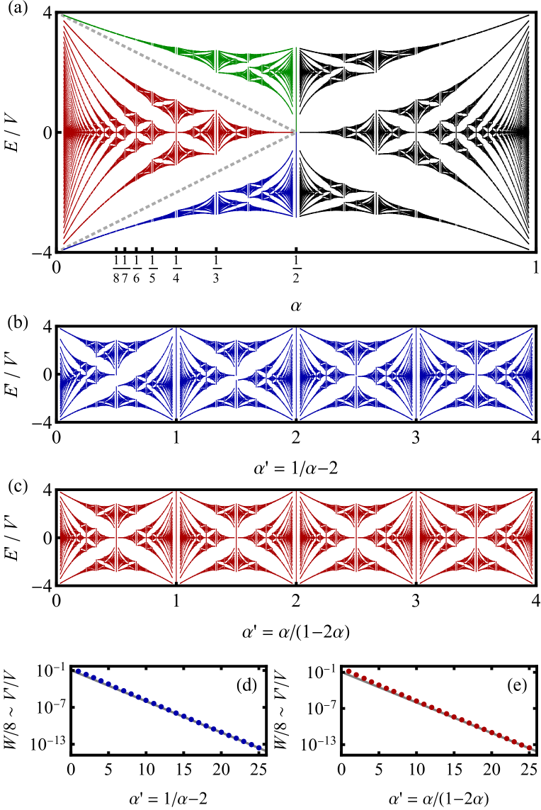
Figure 1: Hofstadter’s butterfly: The spectrum of (3) is plotted (a) for all $\alpha=p/q$ with $q\leq 100$. For $\alpha\in[0,1/2]$ the upper (green), central (red), and lower (blue) Hofstadter bands are shaded. The bands are demarcated by the lines $E/V=\pm(4-8\alpha)$ (grey). The bands are re-plotted (b,c) as a function of $\alpha^{\prime}$, and shifted/rescaled energies $E^{\prime}$, where they produce copies of (a) up to corrections that are small in $\alpha^{\prime}$. In (d,e) the corresponding energetic rescaling is plotted.

Bandstructure for rational $\alpha$:

The spectrum of $H$ consists of the eigenenergies of $H_{\mathrm{AA}}(x_{0})$ calculated for all $x_{0}$. Plotted versus $\alpha$ the spectrum forms a well-known fractal Hofstadter’s butterfly Hofstadter (1976) (Fig. 1). We first discuss some properties of the spectrum which underpin the RG transformation.

For irrational $\alpha$, the spectrum forms a Cantor set Avila and Jitomirskaya (2006); Damanik (2009). However, for rational $\alpha$ ($\alpha=p/q$ for coprime $p,q$) $H_{\mathrm{AA}}$ is $q$-site periodic, and the spectrum consists of bands $j=1\ldots q$ with energies $E_{j}(x_{0},y_{0})$. Here $y_{0}$ (dual to $x_{0}$) is the crystal momentum. $E_{j}(x_{0},y_{0})$ is doubly-periodic with a “Brillouin zone” $(x_{0},y_{0})\in[-\pi/q,\pi/q]^{2}$.

Each band $E_{j}$ has a simple dependency on $(x_{0},y_{0})$, closely resembling the original potential $V(x,y)$. This self similarity underpins the RG treatment. Precisely, each band takes a form Chambers (1965); Bellissard and Simon (1982); Thouless (1983); Wilkinson (1984, 1987); Thouless (1990, 1990); Last (1994); Last and Wilkinson (1992)

$$E_{j}(x_{0},y_{0})=E_{j}^{*}-2V_{x}^{\prime}\cos qy_{0}-2V_{y}^{\prime}\cos qx_{0}+O(W_{j}^{2}/\Delta_{j})$$ (6)

(see App. A) where $|V_{x}^{\prime}/V_{y}^{\prime}|=|V_{x}/V_{y}|^{q}$, $\Delta_{j}$ is the gap to the next band and $W_{j}$ is the bandwidth.

A useful limit in which the corrections to (6) are vanishing is the critical point $V=V_{x}=V_{y}$, for $p=1$, and $q$ large. We will see that this case dominates the scaling behaviour of the curvature of the lowest band. In this limit the gaps scale as $q^{-1}$, whereas the bandwidths are exponentially small Wilkinson (1984, 1987)

$$\Delta_{j}\sim V/[q\,\varrho(E_{j}^{*}/V)],\quad\log W_{j}\sim-q\,\ell(E_{j}^{*}/V).$$ (7)

Here $\varrho(z)$ and $\ell(z)$ are dimensionless, positive, even, $q$-independent functions which are finite and smooth for all $z\neq 0$  (see App. B). By (7) the corrections to (6) vanish at large $q$ for all energies $E_{j}^{*}\neq 0$.

Eq. (6) can be understood as a rescaled HH model. Specifically, if we define rescaled lengths $\hat{x}^{\prime}=qx_{0}$, $\hat{y}^{\prime}=qy_{0}$, then $H^{\prime}=E_{j}(\hat{x}^{\prime},\hat{y}^{\prime})$ is the renormalized Hamiltonian obtained by projecting into the $j$th band. $H^{\prime}$ may similarly be written in tight-binding form (4) using an appropriate Wannier basis Suslov (1982); Szabó and Schneider (2018). Note that $H^{\prime}$ is a copy of the original model (3) for the trivial case of $\alpha^{\prime}=0$. This copy differs by a rescaling of time be $\tau=V/V^{\prime}=8V/W_{j}$, and length by $\lambda=q$. The control parameter transforms as $\delta^{\prime}=\log|V_{x}^{\prime}/V_{y}^{\prime}|=q\delta$, leading to the scaling behvaiour (5).

The above arguments show the bandstructure takes a simple form for $\alpha=1/q$ as $q\to\infty$. Similar arguments apply for $\alpha$ approaching other rationals. For example, consider $q=2p+1$. At large $q$, $\alpha\to 1/2$. In this limit too, the bandwidths are exponentially small $\log W_{j}=O(-q)$, whereas the band gaps decay as $\Delta_{j}=O(q^{-1})$ (see App. B). Thus, here too, the corrections to (6) are vanishing in $q$. We find this case dominates scaling behaviour of the heat capacity of a half-filled Fermi gas.

RG transformation:

As seen above, for rational values of $\alpha$, projecting into a single band of the HH model yielded a rescaled HH model with $\alpha^{\prime}=0$. In fact, this is a special case of an RG transformation which applies for all $\alpha$, and generically yields a renormalised $\alpha^{\prime}\neq 0$.

The RG transformation consists of a projection into a Hofstadter band. Hofstadter bands generalize the notion of bands to the case of irrational $\alpha$. The spectrum consists of three Hofstadter bands, highlighted in Fig. 1a for $\alpha\in[0,1/2]$, these bands extend to $\alpha\in[1/2,1]$ by symmetry under $\alpha\to 1-\alpha$. Using this symmetry, without loss, we work in terms of $\bar{\alpha}:=\min(\alpha,1-\alpha)$. As in (6), projecting into a Hofstadter band yields a HH model with renormalized parameters, plus corrections of $O(W_{j}^{2}/\Delta_{j})$.

The RG step depends on whether one projects into one of the two outer bands, or the central band. For an outer band, we obtain a rescaling of the lattice length

$$a\to a^{\prime}=a\lambda(\bar{\alpha}),$$ (8a)

with scale factor $$\lambda(z)=1/z$$; a renormalized flux density

$$\bar{\alpha}\to\bar{\alpha}^{\prime}=B(\bar{\alpha}):=\min[b(\bar{\alpha}),1-b(\bar{\alpha})],$$ (8b)

where $$b(z):=s(z)-\lfloor s(z)\rfloor s(z)=1/z s(\bar{\alpha})$$ with  ; and an energy rescaling, given in the limit of large by

$$\log V\to\log V^{\prime}\sim\log V-4Gs(\bar{\alpha})/\pi$$ (8c)

where $G=0.9159\ldots$ is Catalan’s constant. Projecting into the central band yields the same RG rules (8c) but with $\lambda(z)=1/(1-2z)$, $s(z)=z/(1-2z)$.

The RG transformation (8c) is obtained from combining the RG analyses of Refs. Suslov (1982); Wilkinson (1984, 1987); Szabó and Schneider (2018) with the Hofstadter rules Hofstadter (1976); Rüdinger and Piéchon (1997), and using symmetry under $\alpha\to 1\pm\alpha$ to work in terms of $\bar{\alpha}\in[0,1/2]$. Note that, for $\bar{\alpha}=1/q$, this RG step recovers the limit (6) and (7) as desired.

The length rescaling (8a) follows from the fraction of states in the Hofstadter bands. At a given $\bar{\alpha}$, a fraction $\bar{\alpha}$ of the spectrum is in each outer band, and the remaining $1-2\bar{\alpha}$ is in the central band Wannier (1978). Thus the rescaling (8a) ensures a fixed spatial density of sites under the RG flow.

The renormalization of $\alpha$ (8b) follows from the Hofstadter rules Hofstadter (1976); Rüdinger and Piéchon (1997). That is, either (i) projecting into one of the outer bands, and sending $\alpha\to\alpha^{\prime}=1/\alpha-2$, or (ii) projecting into the central band, and sending $\alpha\to\alpha^{\prime}=\alpha/(1-2\alpha)$, followed in either case by an appropriate $\alpha^{\prime}$-dependent energy shifts/rescaling, yields a copy of the Hofstadter spectrum up to corrections that are small in $\alpha^{\prime}$. This is shown in Figs. 1b, 1c where the lower (blue) and central (red) Hofstadter bands are replotted in terms of $\alpha^{\prime}$ with energies shifted/rescaled to match the envelope of the bare spectrum. The visible discrepancy in Fig. 1b decays rapidly with $\alpha^{\prime}$. Eq. (8b) is obtained by recasting these relations in terms of $\bar{\alpha}\in[0,1/2]$.

The energy rescaling (8c) can be calculated using WKB methods Szabó and Schneider (2018); Wilkinson (1984, 1987); Han et al. (1994), and is numerically verified in Figs. 1d, 1e. Specifically, the energy rescalings used to produce Fig 1b, 1c are plotted for integer $\alpha^{\prime}$ (coloured points), and converges to the theoretically predicted asymptote (grey line) (8c).

Curvature of the lowest band:

Consider the curvature of the minimum of the lowest Bloch band of $H_{\mathrm{AA}}$

$$\Gamma=\left.\frac{d^{2}E_{0}}{dy_{0}^{2}}\right|_{y_{0}=y_{0,\min}}.$$ (9)

This quantity measures the energetic change of low energy particles due to imposing a current. Moreover, in the many boson generalization of (4), the generalization of (9) determines the superfluid fraction Schultka and Manousakis (1994); Lieb et al. (2002); Roth and Burnett (2003); Cestari et al. (2010); Szabó and Schneider (2018). In the delocalized phase ($\delta<0$) $\Gamma$ takes a finite value, whereas in the localized phase ($\delta>0$) $\Gamma=0$. In the vicinity of the critical point we find scaling

$$\Gamma\sim\xi^{2-z(\zeta,\xi)}\sim\delta^{\nu[z(\zeta,\delta)-2]},\qquad\zeta=48G/\pi^{3}$$ (10)

with $z(\zeta,\delta)$ as in (2).

To obtain (10) we consider the finite size scaling of $\Gamma$, found by taking a series of rational approximations to $\alpha$ which converge $p/q\to\alpha$ at large $q$. In the localized and delocalized phases the finite size approximation $\Gamma(q,\delta)$ converges exponentially $\log|\Gamma(q,\delta)-\Gamma(\infty,\delta)|=O(-q|\delta|)$. In the vicinity of the critical point, for almost all $\alpha\in[0,1]$, we will show $\Gamma$ scales as

$$\Gamma(q,\delta)\sim q^{2-z(\zeta,q)}\mathcal{G}(q^{1/\nu}\delta).$$ (11)

Eq. (10) follows from (11) by taking the limit of $q\to\infty$ using that the critical scaling ceases for $q\gtrsim\xi$.

We now explain how (11) is obtained. At the critical point, the energy of the lowest band varies by $\Delta E=W_{0}$ across a range of momentum $\Delta k_{x}=1/q$ (see e.g. (6)) yielding a curvature of $\Gamma(q,0)=O(W_{0}q^{2})$. The scaling of the quantity $W_{0}q^{2}$ may then be calculated from an RG in which we project into the lower Hofstadter band at every step using the RG rule (8c).

We obtain exact results for the RG by using that the map $B(\bar{\alpha})$, which renormalizes the flux density, is ergodic. Let $\bar{\alpha}_{n}=B^{n}(\bar{\alpha})$ be the sequence of renormalized flux densities obtained by projecting into the lowest band at every RG step. This sequence $\bar{\alpha}_{n}$ approaches the same distribution for almost all initial values of $\bar{\alpha}$

$$f_{n}(\bar{\alpha}):=\frac{1}{n}\sum_{m=0}^{n-1}\delta(\bar{\alpha}-\bar{\alpha}_{m})\sim f(\bar{\alpha})=\frac{\varphi^{3}/\log\varphi}{\varphi^{3}+\bar{\alpha}-\bar{\alpha}^{2}}$$ (12)

where here $\sim$ indicates convergance in distribution at large $n$, and $\varphi=(1+\sqrt[\ ]{5})/2$ is the golden ratio (see App. C). The convergence $f_{n}\to f$ is shown in Fig. 2b.

The ergodicity of $B$ leads to identical dynamical scaling for almost all $\bar{\alpha}$. Consider the length rescaling $\lambda=a_{n}/a_{0}$ after $n$ RG steps: $\lambda=\lambda_{1}\lambda_{2}\cdots$, with $\lambda_{m}=\lambda(\bar{\alpha}_{m})$

$$\log\lambda=\sum_{m=1}^{n}\log\lambda_{m}\sim n\int_{0}^{1/2}\!\!\!\!d\bar{\alpha}f(\bar{\alpha})\log\lambda(\bar{\alpha})=\frac{\pi^{2}n}{12\log\varphi}.$$ (13)

Using that the RG step (8c) is asymptotically exact at small $\bar{\alpha}$, we also obtain an asymptotically exact form for the time (energy) rescaling $\tau=V_{0}/V_{n}$

$$\log\tau\sim\frac{4G}{\pi}\sum_{m=0}^{n-1}s(\bar{\alpha}_{m})=\frac{4Gn}{\pi}\int_{0}^{1/2}d\bar{\alpha}f_{n}(\bar{\alpha})s(\bar{\alpha}).$$ (14)

The asymptotic equality (14) follows as (8c) is asymptotically accurate at small $\bar{\alpha}$, and the sum in (14) is dominated by small $\bar{\alpha}_{m}$. Unlike for the length scaling, the integral in (14) does not converge, but is dominated by the smallest values of $\bar{\alpha}_{n}$ so far. As the limiting distribution $f(\bar{\alpha})$ is finite as $\bar{\alpha}\to 0$, we have $\min_{m<n}\bar{\alpha}_{m}=O(n^{-1})$, and the correct asymptotic scaling is thus

$$\log\tau\sim\frac{4Gn}{\pi}\int_{O(n^{-1})}^{1/2}\!\!\!d\bar{\alpha}\,f(\bar{\alpha})s(\bar{\alpha})=\frac{4Gn\log n}{\pi\log\varphi}+O(n)$$ (15)

The dynamical scaling is then obtained using (13) and (15) and eliminating $n$ to obtain (2) with

$$\zeta=48G/\pi^{3}.$$ (16)

This scaling is shown in Fig 2a. The scaling (11) at $\delta=0$ follows from $\Gamma(q,0)=O(W_{0}q^{2})$ with $q=O(a_{n})$ and $W_{0}=O(V_{n})$. The $\delta$-dependence is fixed by (5).

The origin of the non-power-law scaling is rare RG steps where the renormalised flux is very small $\bar{\alpha}_{n}\ll 1$, which are associated with a large dynamical exponent $z_{n}$. Recasting (13) and (14) in the form of (1) we obtain an exponent for the $n$th RG step given by

$$z_{n}=z(\bar{\alpha}_{n}),\quad z(\bar{\alpha})\sim\frac{4Gs(\bar{\alpha})}{\pi\log\lambda(\bar{\alpha})}=\frac{4G}{\pi|\bar{\alpha}\log\bar{\alpha}|}$$ (17)

which has a non-integrable divergence at small $\bar{\alpha}$. This causes the sum in (14) to grow faster than $O(n)$.

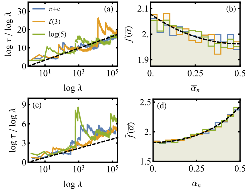
Figure 2: Non-power-law scaling: The time and length rescalings $\tau$ and $\lambda$ are calculated from the RG (8c) (treating (8c) as an equality) after each RG step for $n=10^{5}$ steps. (a,b) shows the lower band RG, and (c,d) the central band RG, for 3 irrational $\alpha$ (legend inset). Plot (a) shows agreement with the predicted scaling $\log\tau=\zeta\log\lambda\log\log\lambda$ with $\zeta=48G/\pi^{3}$ (black, dashed). Fluctuations about the dashed line, though apparent, are asymptotically subleading. (b) shows the convergence of $f_{n}(\bar{\alpha})$ to (12). (c,d) shows the same for the central band RG with $\zeta=32G/3\pi^{3}$ and $f_{n}(\bar{\alpha})$ converging to (21).

Heat capacity of Fermi gas at half filling:

The non-power law scaling uncovered in the previous section is not a special feature of the lowest band. As an example of consider promoting (4) to a system of non-interacting free fermions at half filling. The low temperature behaviour of the specific heat in this system is given by

$$c=\frac{du}{dT}=\frac{d}{dT}\int_{-\infty}^{\infty}\!\!\!dE\,E\,\rho(E)\,n_{\mathrm{F}}(E)$$ (18)

where $u$ is the energy density, $n_{\mathrm{F}}(E)=1/(\mathrm{e}^{E/T}+1)$ is the Fermi-Dirac distribution, and $\rho(E)$ is the density of states (DOS) of $H_{\mathrm{AA}}$. The low temperature $T$ behaviour of $c$ is set by the scaling of $\rho(E)$ as $E\to 0$. At the critical point we find the DOS scaling behaviour

$$N(\tau E)\sim\tau^{1/z(\zeta,\tau)}N(E)$$ (19)

where $N(E)=\int_{-E}^{E}\rho(E^{\prime})dE^{\prime}$ is the integrated DOS, $\sim$ indicates asymptotic equality in the limit of small $E$ and small $\tau$, and $z(\zeta,\lambda)$ is given by (2) with $\zeta=32G/3\pi^{3}$. Making the substitution $x=E/T$ to (18) and using (19) to write $\rho(xT)\sim T^{-1+1/z(\zeta,\tau)}\rho(x)$, we scale out the $T$-dependence to obtain the low-$T$ specific heat scaling

$$c\sim k\,T^{1/z(\zeta,T)},\qquad\zeta=32G/3\pi^{3}.$$ (20)

for $T$ independent $k$.

We obtain the low energy form for the DOS (19) from the RG (8c) projecting into the middle band at each step. After $n$ steps, we have a renormalized energy and length scales of $V_{n}$, and $a_{n}$ which determine the low energy behaviour of the DOS via the relation $N(4V_{n})=a_{0}/a_{n}$.

The RG for the middle band proceeds according to (8c) with $s(z)=z\lambda(z)=z/(1-2z)$. To obtain analytic results, instead of taking one RG step at a time, we take “RG super-steps” consisting of $r$ RG steps, where $r(\bar{\alpha}):=\lfloor 1/(2\bar{\alpha})\rfloor$ is determined by $\bar{\alpha}$ . Under one super-step the renormalization rules (8c) hold with the replacements $\lambda(z)\to\tilde{\lambda}(z)=1/(1-2zr(z))$ and $s(z)\to\tilde{s}(z)=z\tilde{\lambda}(z)$ (throughout tilde denotes the RG super-step). The analysis then proceeds as in the previous section. The super-step flux renormalization map $\tilde{B}(\bar{\alpha})$ is ergodic, so that the $\bar{\alpha}_{m}:=\tilde{B}^{m}(\bar{\alpha})$ converge to a steady state distribution

$$\tilde{f}_{n}(\bar{\alpha}):=\frac{1}{n}\sum_{m=0}^{n-1}\delta(\bar{\alpha}-\bar{\alpha}_{m})\sim\tilde{f}(\bar{\alpha})=\frac{2}{\log 3}\,\frac{1}{1-\bar{\alpha}^{2}}.$$ (21)

For a single middle band RG step, the dynamical exponent $z_{n}=z(\bar{\alpha}_{n})$ diverges as $\bar{\alpha}_{n}\to 1/2$, rather than $\bar{\alpha}\to 0$ as before. Otherwise, the analysis proceeds by direct generalization, and yields length and time rescalings

$$\log\lambda=\log\frac{\tilde{a}_{n}}{\tilde{a}_{0}}\sim\frac{\pi^{2}n}{4\log 3},\quad\log\tau=\log\frac{\tilde{V}_{0}}{\tilde{V}_{n}}\sim\frac{8Gn\log n}{3\pi\log 3}$$ (22)

from which we obtain the dynamical scaling (2) (see Fig. 2c). Combining (22) with the low energy behaviour $N(4V_{n})=a_{0}/a_{n}$ we obtain the low energy scaling of the DOS (19) and hence the specific heat scaling (20).

Discussion

We have shown that, in the critical HH model, for almost all $\alpha$, the scaling of the lowest bandwidth (9), and the heat capacity of a half filled Fermi gas (18) both exhibit the now-power law length-energy scaling (2) with respective coefficients $\zeta=48G/\pi^{3}$, and $\zeta=32G/3\pi^{3}$ where $G$ is Catalan’s constant.

Our results hold for almost all $\alpha$. They thus extend previous analyses of critical scaling in incommensurate systems Han et al. (1994); Kohmoto and Banavar (1986); Fujiwara et al. (1989); Hiramoto and Abe (1988b, a); Hiramoto and Kohmoto (1992); Kohmoto et al. (1987); Hiramoto and Kohmoto (1992); Gopalakrishnan (2017); Devakul and Huse (2017); Levitov (1989); Kohmoto et al. (1983); Ostlund and Pandit (1984); Würtz et al. (1988) which focus on specific values of $\alpha$, often quadratic integers (e.g. metallic ratios). For quadratic integers, the orbit $\bar{\alpha}_{n}$ is periodic in $n$. Quadratic integers are thus instances of the measure zero exceptions to our result (2), and have power law dynamical scaling.

The RG employed is generically only approximate in a single step, however it is asymptotically exact in the respective limits $\bar{\alpha}\to 0$ ($\bar{\alpha}\to 1/2$) in the two cases studied. These limits are found to dominate the RG, resulting in an asymptotically exact dynamical scaling. That is, the errors induced are asymptotically subleading, and do not affect the asymptotic equality (2).

Two key features of the RG underpin the $\alpha$-independent non-power-law scaling (2): (i) $\bar{\alpha}$ is renormalized by an ergodic map $B$, causing the distribution of $\bar{\alpha}_{n}$ to converge to the same distribution $f(\bar{\alpha})$ independent of $\bar{\alpha}_{0}$, and (ii) that as $\bar{\alpha}_{n}$ approaches some rational $\bar{\alpha}^{*}$ the single step dynamical exponent $z_{n}=z(\bar{\alpha}_{n})$ has a non-integrable divergence. Consequently, rare large values of $z_{n}$ dominate the dynamical scaling.

We expect this scaling (2) uncovered here is generic for a broad class of critical models. Specifically, consider a generalized HH model $H_{\mathrm{G}}=V_{s}(\hat{x},\hat{y})$ where $V_{s}$ is any smooth function periodic in its two arguments, and $s$ is a tuning parameter. $V_{s}$ forms a periodic potential, whose equipotentials, are either closed or open. Generically (i.e. away from critical points) a finite fraction of the equipotentials are open, all of which extend parallel to a particular lattice vector $\vec{b}$. As $s$ is varied, there are critical points where $\vec{b}$ discretely changes. At these points $H_{\mathrm{G}}$ is critical, and generalises the critical HH model.

The spectrum of the critical generalized HH model forms a fractal, analogous to Hofstadter’s butterfly (Fig. 1), and an analogous RG transformation can be constructed. Under this RG we expect the dynamical scaling (2) with a $\alpha$-independent value of $\zeta$ provided it preserves the properties (i) and (ii) above. Property (i) follows as by zooming in on a point in the spectrum, the RG transformation necessarily amplifies small changes to the initial value of $\alpha$, i.e. it is always chaotic, and thus one expects it is ergodic too. Property (ii) follows by direct generalization of the WKB methods used to show this property in the Hofstadter model Szabó and Schneider (2018); Wilkinson (1984, 1987); Han et al. (1994), which require only that $V(x,y)$ is smooth.

We leave to further work the exploration of the implications of this non-power law dynamic scaling for wavepacket spreading Ketzmerick et al. (1997); Piéchon (1996), and extension to the analysis of symmetry breaking transitions, rather than the metal-insulator transition studied here. One may approach the latter case using certain models of the form $H_{\mathrm{G}}$, which map onto quasiperiodic Ising chains Ceccatto (1989); Benza (1989); Luck (1993); Chandran and Laumann (2017); Crowley et al. (2018a, b).

Acknowledgements

We are grateful for useful discussions with A. Szabó, and to C. Murthy for useful comments on a draft. P.C. is supported by the NSF STC “Center for Integrated Quantum Materials” under Cooperative Agreement No. DMR-1231319.

Appendix A Derivation of Eq. (6)

In this section we derive (6), that the energetic dependence of a single band of the HH model for rational flux $\alpha=p/q$ is given by

$$E_{j}(x_{0},y_{0})=E_{j}^{*}-2V_{x}^{\prime}\cos qy_{0}-2V_{y}^{\prime}\cos qx_{0}+O(W_{j}^{2}/\Delta_{j}).$$ (23)

In the related, AA model the quantities $(x_{0},y_{0})$ have a straightforward interpretation: $x_{0}$ acts as the phase of the potential, and $y_{0}$ is a crystal momentum, and vice versa in the dual model obtained by writing in the $y$-basis. The results of this section are obtained using well known properties of the characteristic equation and spectrum of the HH model Chambers (1965); Bellissard and Simon (1982); Thouless (1983, 1990, 1990); Last (1994); Last and Wilkinson (1992).

Our first step is to obtain a useful form for the characteristic equation, the roots of which are the bands $E_{j}(x_{0},y_{0})$. We begin by noting that, per (4), when written in the $x$-basis $\hat{x}|x\rangle=x|x\rangle$ the HH hamiltonian takes the form $H=\int_{0}^{2\pi\alpha}dx_{0}H_{\mathrm{AA}}(x_{0})$ with

$$H_{\mathrm{AA}}(x_{0}) =\sum_{n\in\mathbb{Z}}\Big{[}V_{y}\left(|x_{0}+2\pi\alpha(n+1)\rangle\langle x_{0}+2\pi\alpha n|+\mathrm{h.c}\right)+2V_{x}\cos x_{n}|x_{0}+2\pi\alpha n\rangle\langle x_{0}+2\pi\alpha n|\Big{]}.$$ (24)

This Hamiltonian is manifestly periodic under a shift $x\to x+2\pi\alpha q$, and so we may project in a momentum sector, in which we obtain the Bloch Hamiltonian

$$H_{\mathrm{B}}(x_{0},y_{0}) =-\sum_{n\in\mathbb{Z}}\Big{[}V_{y}\left(\mathrm{e}^{iy_{0}}|n+1\rangle\langle n|+\mathrm{h.c}\right)+2V_{x}\cos x_{n}|n\rangle\langle n|\Big{]}$$ (25)

where we identify $|n\rangle\equiv|n+q\rangle$. The spectrum of $H$ is thus made up of bands $E_{j}(x_{0},y_{0})$ determined by the solutions of the characteristic equation

$$C(E_{j}(x_{0},y_{0}),x_{0},y_{0})=0$$ (26)

where $C$ is the characteristic polynomial given by

$$C(E,x_{0},y_{0}):=\det(H_{\mathrm{B}}(x_{0},y_{0})-E).$$ (27)

Remarkably, the characteristic polynomial has a very simple dependence on $x_{0},y_{0}$

$$C(E,x_{0},y_{0})=P(E)+C_{0}(x_{0},y_{0})$$ (28)

where $P(E)$ is a $q$th order polynomial independent of $x_{0}$ and $y_{0}$, and $C_{0}$ is an energy independent constant

$$P(E) =\det(H_{\mathrm{B}}(\pi/2q,\pi/2q)-E)$$ (29)

$$C_{0}(x_{0},y_{0}) =-2V_{x}^{q}\cos qx_{0}-2V_{y}^{q}\cos qy_{0}.$$

Hence the roots of the characteristic polynomial are the solutions to the equation

$$P(E)=-C_{0}(x_{0},y_{0}).$$ (30)

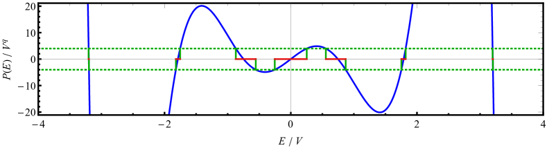
Figure 3: Graphical illustration of solutions to (30) for $V_{x}=V_{y}=V$ and $\alpha=p/q=1/7$: $P(E)$ is shown in blue, the range of values swept out by $C_{0}$ is demarcated by the dashed green lines, and the corresponding range of values swept out by the roots of (30) is marked in red on the horizontal axis.

The solutions to (30) are plotted in Fig 3 for $V_{x}=V_{y}=V$ and $\alpha=1/7$. In this figure $P(E)$ is shown in blue, the range of values swept out by $C_{0}$ is demarcated by the dashed green lines, and the corresponding range of values swept out by the solutions to (30) is marked in red on the horizontal axis. Each red interval corresponds to one band $E_{j}(x_{0},y_{0})$. Intuitively, it follows from eyeballing Fig. 3 that each band takes the form

$$E_{j}(x_{0},y_{0})\approx E_{j}^{*}+\frac{C_{0}(x_{0},y_{0})}{P^{\prime}(E_{j}^{*})}$$ (31)

which may be obtained by linearizing $P(E)$ about its roots $E_{j}^{*}$. We expect the corrections to this to be small if the variation of the gradient $P^{\prime}(E)$ is small over the interval in which $E_{j}(x_{0},y_{0})$ varies, i.e. to leading order, that $W_{j}P^{\prime\prime}(E_{j}^{*})\ll P^{\prime}(E_{j}^{*})$ where $W_{j}$ is the bandwidth. There is reason to expect this leading order analysis of the error should be expected to provide an accurate answer: $P^{\prime\prime}(E)$ varies only on the scale of the separation between successive roots, and thus we generically expect $P^{\prime\prime}(E_{j}^{*})$ to provide a good order of magnitude estimate for $P^{\prime\prime}(E)$ for $E$ in the range $E_{j-1}^{*}\leq E\leq E_{j+1}^{*}$. In the remainder of this section, we perform such a leading order analysis to make intuitive statement more precise.

Having obtained a form for the characteristic equation, we see that linearizing $P(E)$ about its roots $E_{j}^{*}$, yields

$$0=P^{\prime}(E_{j}^{*})(E_{j}(x_{0},y_{0})-E_{j}^{*})+C_{0}(x_{0},y_{0})+O(P^{\prime\prime}(E_{j}^{*})(E_{j}(x_{0},y_{0})-E_{j}^{*})^{2}).$$ (32)

The solutions to this equation give the band structure up to an error which must be estimated

$$E_{j}(x_{0},y_{0}) =E_{j}^{*}+\frac{C_{0}(x_{0},y_{0})}{P^{\prime}(E_{j}^{*})}-O\left(\frac{C_{0}^{2}(x_{0},y_{0})P^{\prime\prime}(E_{j}^{*})}{(P^{\prime}(E_{j}^{*}))^{3}}\right)$$ (33)

$$=E_{j}^{*}-2V_{x}^{\prime}\cos qx_{0}-2V_{y}^{\prime}\cos qy_{0}-O\left(\frac{W_{j}^{2}P^{\prime\prime}(E_{j}^{*})}{P^{\prime}(E_{j}^{*})}\right)$$

where in the second line we have substituted (30) and defined $V_{x}^{\prime}=V_{x}^{q}/P^{\prime}(E_{j}^{*})$, $V_{y}^{\prime}=V_{y}^{q}/P^{\prime}(E_{j}^{*})$ and $W_{j}=4V_{x}^{\prime}+4V_{y}^{\prime}$

Finally, we note that the ratio $P^{\prime\prime}(E_{j}^{*})/P^{\prime}(E_{j}^{*})$ may be related to the band spacing. Specifically, for a quadratic expansion of the characteristic polynomial

$$P(E)=P^{\prime}(E_{j}^{*})(E_{j}(x_{0},y_{0})-E_{j}^{*})-C_{0}(x_{0},y_{0})+\tfrac{1}{2}P^{\prime\prime}(E_{j}^{*})(E_{j}(x_{0},y_{0})-E_{j}^{*})^{2}+O(P^{\prime\prime\prime}(E_{j}^{*})(E_{j}(x_{0},y_{0})-E_{j}^{*})^{3})$$ (34)

this equation has roots at

$$E=E_{j}^{*},\qquad\text{and}\qquad E=E_{j}^{*}-\frac{2P^{\prime}(E_{j}^{*})}{P^{\prime\prime}(E_{j}^{*})}+O\left(\frac{P^{\prime}(E_{j}^{*})^{2}P^{\prime\prime\prime}(E_{j}^{*})}{P^{\prime\prime}(E_{j}^{*})^{2}}\right)$$ (35)

this yields and distance between the roots of

$$\Delta_{j}=\frac{2P^{\prime}(E_{j}^{*})}{P^{\prime\prime}(E_{j}^{*})}+O\left(\frac{P^{\prime}(E_{j}^{*})^{2}P^{\prime\prime\prime}(E_{j}^{*})}{P^{\prime\prime}(E_{j}^{*})^{3}}\right)$$ (36)

which, combined with (33), yields (6) in the main text.

Appendix B Numerical evidence of Eq. (7)

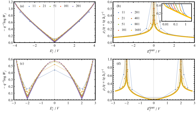
Figure 4: Limiting forms for the bandwidths $W_{j}$ and band gaps $\Delta_{j}$: (a,b) the bandwidths and band gaps are analysed for $\alpha=1/q$ in the limit $q\to\infty$ (a) $q^{-1}\log W_{j}$ is plotted versus $E_{j}^{*}$ for various values of $q$ (legend inset), in (b) $(\Delta_{j}q)^{-1}$ is plotted versus $E_{j}^{(\mathrm{gap})}$, the inset shows the same data on a logarithmic horizontal scale. In (c,d) analogous plots are shown for $\alpha=p/q$ with $q=2p+1$.

Eq. (7) is obtained via anayltic arguments by Wilkinson in Refs. Wilkinson (1984, 1987). Nevertheless, here we provide some numerical evidence of this result.

Consider the HH Hamiltonian (3) with $\alpha=1/q$ tuned to the critical point $V_{x}=V_{y}=V$. Per the previous Appendix, this Hamiltonian has $q$ bands $E_{j}(x_{0},y_{0})$ for $j=1\cdots q$. We denote the extrema of each band by $E_{j}^{(\min)}$ and $E_{j}^{(\max)}$. We further denote the band centers, bandwidths, and gap centers respectively by

$$E_{j}^{*}=\tfrac{1}{2}\left(E_{j}^{(\max)}+E_{j}^{(\min)}\right),\qquad\Delta_{j}=\rho_{j}^{-1}=E_{j+1}^{(\min)}-E_{j}^{(\max)},\qquad E_{j}^{(\mathrm{gap})}=\tfrac{1}{2}\left(E_{j+1}^{(\min)}+E_{j}^{(\max)}\right)$$ (37)

where $\rho_{j}=\Delta_{j}^{-1}$ is the density of states at the gap center.

In Fig. 4a we show the bandwidths are decaying exponentially in $q$, specifically we plot $q^{-1}\log W_{j}$ versus $E_{j}^{*}$ for various values of $q$ (legend inset). The different $q$ series approaches a limiting form at large $q$

$$\log W_{j}\sim-q\ell(E_{j}^{*}/V).$$ (38)

In Fig. 4b we plot $\rho_{j}/q$ as a function of $E_{j}^{(\mathrm{gap})}$, showing that in the same limit the density of states has the limiting form

$$\rho_{j}=\Delta_{j}^{-1}\sim q\varrho(E_{j}^{*}/V)/V.$$ (39)

In the inset of Fig. 4b the same data is shown on a log scale, showing that $\varrho(z)$ has an integrable (specficially logarithmic) divergence at $z=0$. Plots Fig. 4c-d show the equivalent plots in the limit of large $q$ with $q=2p+1$, illustrating that analgous limits occur for $\alpha\to 1/2$. Indeed similar limits apply for $\alpha$ approaching any rational.

Appendix C The ergodic map $B(\bar{\alpha})$

In this section we show the ergodicity of the map $B:[0,1/2]\to[0,1/2]$ corresponding to an RG where we project into the lower band at each step. That, for $B$ given by

$$B(\bar{\alpha})=\min\left[b(\bar{\alpha}),1-b(\bar{\alpha})\right],\qquad b(\bar{\alpha})=\frac{1}{\bar{\alpha}}-\left\lfloor\frac{1}{\bar{\alpha}}\right\rfloor,$$ (40)

as defined in the main text in Eq. (8b). Results for an RG projecting into the middle band at each step, as used in the latter part of the paper, follow by the same methods.

We employ a numerical approach previously used in Ref. Briggs (2003); Flajolet and Vallée (1995) to calculate the spectral gap of the Gauss map. Consider an initial set values $\bar{\alpha}_{0}^{(i)}\in[0,1/2]$ characterized by a smooth distributed $g_{0}(\bar{\alpha})$. Each of these values can be renormalized to yield $\bar{\alpha}_{n}^{(i)}=B^{n}(\bar{\alpha}_{0}^{(i)})$, which is also characterised by a smooth distribution function $g_{n}(\bar{\alpha})$. As $n$ is taken large $g_{n}$ converges to the unique steady state distribution

$$g_{n}(\bar{\alpha})\to f(\bar{\alpha})=\frac{1}{\log\varphi}\cdot\frac{\varphi^{3}}{\varphi^{3}+\bar{\alpha}-\bar{\alpha}^{2}}$$ (41)

where $\varphi=(1+\sqrt[\ ]{5})/2$ is the golden ratio. Moreover, the deviation from the limiting distribution is exponentially small in $n$

$$\log|g_{n}(\bar{\alpha})-f(\bar{\alpha})|\sim-n\Delta,$$ (42)

where

$$\Delta=3.7856665519818449128\ldots$$ (43)

is the spectral gap of $B$. The statement (42) together with $\Delta>0$ demonstrates the ergodicity of the map $B$. Moreover, the large value $\Delta\gg 1$, indicates that the convergence of $g_{n}(x)$ to $f(x)$ occurs rapidly over an $O(1)$ number of steps. Eq. (42) is the main result of this section. Prior to the main result, we arrive at two further results: (i) we show that $f(\bar{\alpha})$ in (41) is the steady state, and (ii) we show that the map $B$ is chaotic with maximal Lyapunov exponent

$$\Lambda=\frac{\pi^{2}}{6\log\varphi}.$$ (44)

C.1 Steady state distribution of $B$

The sequence of distributions $g_{n}$ are defined by recursive application of the map $B$, i.e. $g_{n+1}(\bar{\alpha})=[Bg_{n}](\bar{\alpha})$, where the action of $B$ on $g$ is given explicitly by

$$(\bar{\alpha}) :=\int_{0}^{1/2}d\bar{\alpha}^{\prime}\delta(\bar{\alpha}-B(\bar{\alpha}^{\prime}))g(\bar{\alpha}^{\prime})=\sum_{q=2}^{\infty}\left[\frac{g\left(\frac{1}{q+\bar{\alpha}}\right)}{(q+\bar{\alpha})^{2}}+\frac{g\left(\frac{1}{q+1-\bar{\alpha}}\right)}{(q+1-\bar{\alpha})^{2}}\right].$$ (45)

Note that the action of $B$ on the space of distributions $g$ is linear, $[B(g+h)]=[Bg]+[Bh]$, and thus the steady state distribution $f$ is obtained as the leading eigenfunction of $B$, which has a corresponding eigenvalue of unity

$$[Bf](\bar{\alpha})=f(\bar{\alpha}).$$ (46)

It is then straightforward to verify that (41) satisfies this relation. The uniqueness of this solution is verified numerically in App. C.3.

C.2 Chaoticity of $B$

The Lyapunov exponent of a discrete map is given by

$$\Lambda=\lim_{n\to\infty}\frac{1}{n}\sum_{m=1}^{n}\log|B^{\prime}(\bar{\alpha}_{n})|$$ (47)

where $\bar{\alpha}_{n}=B^{n}(\bar{\alpha}_{0})$, $B^{\prime}(\bar{\alpha})$ is the derivative of $B(\bar{\alpha})$ and the Lyapunov exponent $\Lambda$ is independent of $\bar{\alpha}_{0}$ due to the ergodicity of $B$.

Moreover, as $B$ is ergodic, $\Lambda$ may be straightforwardly evaluated using the steady state distribution $f(\bar{\alpha})$

$$\Lambda =\int_{0}^{1/2}d\bar{\alpha}\,f(\bar{\alpha})\,\log|B(\bar{\alpha})|=-2\int_{0}^{1/2}d\bar{\alpha}\,f(\bar{\alpha})\,\log\bar{\alpha}=\frac{\pi^{2}}{6\log\varphi}$$ (48)

In Eq. (48) we have used that $|B(\bar{\alpha})|=\bar{\alpha}^{-2}$ except at a measure zero set of points, where the derivative is undefined. As $\Lambda>0$, $B$ is chaotic.

C.3 Ergodicity of $B$

As $B$ is a linear operator, it has a spectrum of eigenvalues $\beta_{k}\geq 0$ with associated eigenfunctions $v_{k}(\bar{\alpha})$ which form a complete basis

$$[Bv_{k}](\bar{\alpha})=\beta_{k}v_{k}(\bar{\alpha}).$$ (49)

In principle the spectrum of eigenvalues may have discrete and continuous components, though in the present case we find only a discrete spectrum allowing us to index them in descending order $1=|\beta_{0}|\geq|\beta_{1}|\geq|\beta_{2}|\geq\cdots$. The distribution at late times is found by projecting onto the subspace of eigenfunctions with eigenvalues $|\beta_{k}|=1$. If there is exactly one such eigenvalue, which we denote as $\beta_{0}=1$ (the eigenvalue cannot have a phase as $g_{n}(\bar{\alpha})$ is strictly non-negative), then the steady state distribution $f(\bar{\alpha})$ is unique, independent of $g_{0}$, and given by the corresponding eigenfunction $f=v_{0}$. The deviation of $g_{n}$ from $v_{0}$ is then determined by the first sub-leading eigenvalue: $|f-g_{n}|=O(\beta_{1}^{n})=O(\mathrm{e}^{-\Delta n})$, where we have defined

$$\Delta=-\log|\beta_{1}|$$ (50)

as the spectral gap of $B$.

The eigenfucntion(s) $v_{k}(\bar{\alpha})$ may be obtained as the solutions to the eigenvalue equation (49), however in the absence of an analytic technique to solve this equation, we resort to numerics. To numerically tackle this problem we first re-write in terms of the coordinate $y=1/2-\bar{\alpha}\in[0,1/2]$. In this coordinate $B$ has the action

$$[Bg](y)=\sum_{h}\left[\frac{g\left(\tfrac{1}{2}-\frac{1}{h-y}\right)}{(h-y)^{2}}+\frac{g\left(\tfrac{1}{2}-\frac{1}{h+y}\right)}{(h+y)^{2}}\right]$$ (51)

where the sum is taken over the half-integers $h=\tfrac{5}{2},\tfrac{7}{2},\tfrac{9}{2},\tfrac{11}{2}\ldots$. To make the problem numerically tractable we subsequently write $B$ in a basis spanned by a countable set of basis elements. For simplicity we choose the basis monomials

$$u_{p}(y)=y^{p}=(1/2-x)^{p}$$ (52)

upon which $B$ acts as

$$(y) =\sum_{h}\frac{1}{2^{p}}\left[\frac{\left(1-\frac{2}{h-y}\right)^{p}}{(h-y)^{2}}+\frac{\left(1-\frac{2}{h+y}\right)^{p}}{(h+y)^{2}}\right]$$ (53)

$$=\sum_{h}\frac{1}{2^{p+2}}\sum_{k=0}^{p}\binom{p}{k}\left(-\frac{2}{h}\right)^{k+2}\left[\left(\frac{1}{1-y/h}\right)^{k+2}+\left(\frac{1}{1+y/h}\right)^{k+2}\right]$$

$$=\sum_{h}\frac{1}{2^{p+2}}\sum_{k=0}^{p}\binom{p}{k}\left(-\frac{2}{h}\right)^{k+2}\left[2\sum_{n=0}^{\infty}\binom{2n+k+1}{2n}\left(\frac{y}{h}\right)^{2n}\right]$$

Recalling the definition of the Hurwitz zeta function $\zeta(s,a)=\sum_{n=0}^{\infty}(n+a)^{-s}$, and rerranging we find

$$[Bu_{p}](y)=\sum_{k=0}^{p}\sum_{n=0}^{\infty}\binom{p}{k}\binom{2n+k+1}{2n}\frac{(-1)^{k}}{2^{p-k-1}}\zeta(2n+k+2,5/2)u_{2n}(y).$$ (54)

We re-write (54) to define $M_{pq}$, the transfer matrix on the basis on monomials $u_{p}$ we

$$[Bu_{p}](y)=\sum_{q=0}^{\infty}M_{pq}u_{q}(y)$$ (55)

where the matrix elements are given by

$$M_{pq}=\begin{cases}\displaystyle\frac{1}{2^{p-1}}\sum_{k=0}^{p}\binom{p}{k}\binom{q+k+1}{q}(-2)^{k}\zeta(q+k+2,5/2)&\qquad q\text{\,\, even},\\[15.0pt] 0&\qquad q\text{\,\, odd}.\end{cases}$$ (56)

The spectrum of $M$, and hence $B$, may then be numerically estimated by evaluating $M_{pq}$ up to a cutoff $p,q\leq p_{\max}$ and diagonalising. The eigenvalues $\beta_{k}$ are found to be discrete, non-degenerate and exponentially decaying in $k$. As a result the values of low order eigenvalues converge exponentially as a function of $p_{\max}$, allowing them to be accurately numerically estimated. The numerical limitation is the evaluation of the matrix elements, which require high precision numerics for even moderately large $p_{\max}$. Numerically extracted values for the magnitudes of the first five sub-leading eigenvalues are given below (to 20 significant figures)

$$-\log|\beta_{0}| =0$$ (57)

$$\Delta=\Delta_{1}=-\log|\beta_{1}| =3.7856665519818449128$$

$$\Delta_{2}=-\log|\beta_{2}| =6.7251453074741971174$$

$$\Delta_{3}=-\log|\beta_{3}| =11.339665867968595165$$

$$\Delta_{4}=-\log|\beta_{4}| =12.043871233196576668$$

$$\Delta_{5}=-\log|\beta_{5}| =16.966376007200018885$$

Indeed, as expected, the associated leading eigenfunction is found to be

$$f(\bar{\alpha})\propto\sum_{q=0}^{\infty}\left(\frac{1-2\bar{\alpha}}{\varphi^{3}}\right)^{2q}$$ (58)

where $\varphi=(1+\sqrt[\ ]{5})/2$ is the Golden Ratio. Performing the sum in (58) and normalising yields (41).

References

- Dean et al. (2013) C. R. Dean, L. Wang, P. Maher, C. Forsythe, F. Ghahari, Y. Gao, J. Katoch, M. Ishigami, P. Moon, M. Koshino, et al., Nature 497, 598 (2013).
- Hunt et al. (2013) B. Hunt, J. D. Sanchez-Yamagishi, A. F. Young, M. Yankowitz, B. J. LeRoy, K. Watanabe, T. Taniguchi, P. Moon, M. Koshino, P. Jarillo-Herrero, et al., Science 340, 1427 (2013).
- Dean et al. (2012) C. R. Dean, L. Wang, P. Maher, C. Forsythe, F. Ghahari, Y. Gao, J. Katoch, M. Ishigami, P. Moon, M. Koshino, et al., arXiv preprint arXiv:1212.4783 (2012).
- Ponomarenko et al. (2013) L. Ponomarenko, R. Gorbachev, G. Yu, D. Elias, R. Jalil, A. Patel, A. Mishchenko, A. Mayorov, C. Woods, J. Wallbank, et al., Nature 497, 594 (2013).
- Andrei and MacDonald (2020) E. Y. Andrei and A. H. MacDonald, Nature materials 19, 1265 (2020).
- Carr et al. (2017) S. Carr, D. Massatt, S. Fang, P. Cazeaux, M. Luskin, and E. Kaxiras, Physical Review B 95, 075420 (2017).
- Roati et al. (2008) G. Roati, C. D’Errico, L. Fallani, M. Fattori, C. Fort, M. Zaccanti, G. Modugno, M. Modugno, and M. Inguscio, Nature 453, 895 (2008).
- Deissler et al. (2010) B. Deissler, M. Zaccanti, G. Roati, C. D’Errico, M. Fattori, M. Modugno, G. Modugno, and M. Inguscio, Nature physics 6, 354 (2010).
- Aidelsburger et al. (2013) M. Aidelsburger, M. Atala, M. Lohse, J. T. Barreiro, B. Paredes, and I. Bloch, Physical review letters 111, 185301 (2013).
- Schreiber et al. (2015) M. Schreiber, S. S. Hodgman, P. Bordia, H. P. Lüschen, M. H. Fischer, R. Vosk, E. Altman, U. Schneider, and I. Bloch, Science 349, 842 (2015).
- Bordia et al. (2017) P. Bordia, H. Lüschen, S. Scherg, S. Gopalakrishnan, M. Knap, U. Schneider, and I. Bloch, Physical Review X 7, 041047 (2017).
- Goldenfeld (2018) N. Goldenfeld, Lectures on phase transitions and the renormalization group (CRC Press, 2018).
- Cardy (1996) J. Cardy, Scaling and renormalization in statistical physics, Vol. 5 (Cambridge university press, 1996).
- Simon (1982) B. Simon, Advances in Applied Mathematics 3, 463 (1982).
- Damanik (2009) D. Damanik, arXiv preprint arXiv:0908.1093 (2009).
- Kohmoto et al. (1983) M. Kohmoto, L. P. Kadanoff, and C. Tang, Physical Review Letters 50, 1870 (1983).
- Ostlund and Pandit (1984) S. Ostlund and R. Pandit, Physical Review B 29, 1394 (1984).
- Würtz et al. (1988) D. Würtz, T. Schneider, and A. Politi, Physics Letters A 129, 88 (1988).
- Levitov (1989) L. Levitov, Journal de Physique 50, 707 (1989).
- Hermisson et al. (1997) J. Hermisson, U. Grimm, and M. Baake, Journal of Physics A: Mathematical and General 30, 7315 (1997).
- Vieira (2005) A. P. Vieira, Physical Review B 71, 134408 (2005).
- Thiem (2015) S. Thiem, Philosophical Magazine 95, 1233 (2015).
- Suslov (1982) I. Suslov, Zh. Eksp. Teor. Fiz 83, 1079 (1982).
- Wilkinson (1984) M. Wilkinson, Proceedings of the Royal Society of London. A. Mathematical and Physical Sciences 391, 305 (1984).
- Wilkinson (1987) M. Wilkinson, Journal of Physics A: Mathematical and General 20, 4337 (1987).
- Szabó and Schneider (2018) A. Szabó and U. Schneider, Physical Review B 98, 134201 (2018).
- Rauh et al. (1974) A. Rauh, G. Wannier, and G. Obermair, physica status solidi (b) 63, 215 (1974).
- Thouless and Niu (1983) D. Thouless and Q. Niu, Journal of Physics A: Mathematical and General 16, 1911 (1983).
- Paul et al. (2022) N. Paul, P. J. Crowley, T. Devakul, and L. Fu, arXiv preprint arXiv:2202.05854 (2022).
- Hofstadter (1976) D. R. Hofstadter, Physical review B 14, 2239 (1976).
- Harper (1955) P. G. Harper, Proceedings of the Physical Society. Section A 68, 874 (1955).
- Thouless (1983) D. Thouless, Physical Review B 28, 4272 (1983).
- Thouless (1990) D. Thouless, Communications in mathematical physics 127, 187 (1990).
- Thouless and Tan (1991) D. Thouless and Y. Tan, Journal of Physics A: Mathematical and General 24, 4055 (1991).
- Wannier (1978) G. Wannier, physica status solidi (b) 88, 757 (1978).
- Han et al. (1994) J. Han, D. Thouless, H. Hiramoto, and M. Kohmoto, Physical Review B 50, 11365 (1994).
- Last and Wilkinson (1992) Y. Last and M. Wilkinson, Journal of Physics A: Mathematical and General 25, 6123 (1992).
- Zilberman (1956) G. Zilberman, JETP 3, 835 (1956).
- Aubry and André (1980) S. Aubry and G. André, Ann. Israel Phys. Soc 3, 133 (1980).
- Azbel (1979) M. Y. Azbel, Phys. Rev. Lett. 43, 1954 (1979).
- Jitomirskaya (1999) S. Y. Jitomirskaya, Annals of Mathematics , 1159 (1999).
- Hiramoto and Abe (1988a) H. Hiramoto and S. Abe, Journal of the Physical Society of Japan 57, 1365 (1988a).
- Ketzmerick et al. (1997) R. Ketzmerick, K. Kruse, S. Kraut, and T. Geisel, Physical review letters 79, 1959 (1997).
- Avila and Jitomirskaya (2006) A. Avila and S. Jitomirskaya, in Mathematical physics of quantum mechanics (Springer, 2006) pp. 5–16.
- Chambers (1965) W. Chambers, Physical Review 140, A135 (1965).
- Bellissard and Simon (1982) J. Bellissard and B. Simon, Journal of functional analysis 48, 408 (1982).
- Last (1994) Y. Last, Communications in mathematical physics 164, 421 (1994).
- Note (1) At , and diverges logarithmically.
- Note (2) Note in this case, is the Gauss map.
- Rüdinger and Piéchon (1997) A. Rüdinger and F. Piéchon, Journal of Physics A: Mathematical and General 30, 117 (1997).
- Schultka and Manousakis (1994) N. Schultka and E. Manousakis, Physical Review B 49, 12071 (1994).
- Lieb et al. (2002) E. H. Lieb, R. Seiringer, and J. Yngvason, in The Stability of Matter: From Atoms to Stars (Springer, 2002) pp. 903–908.
- Roth and Burnett (2003) R. Roth and K. Burnett, Physical Review A 68, 023604 (2003).
- Cestari et al. (2010) J. C. C. Cestari, A. Foerster, and M. Gusmao, Physical Review A 82, 063634 (2010).
- Note (3) When taking single RG steps, one finds most RG steps have resulting in insignificant rescaling of length and time. Taking RG super-steps addresses this pathology.
- Kohmoto and Banavar (1986) M. Kohmoto and J. R. Banavar, Physical Review B 34, 563 (1986).
- Fujiwara et al. (1989) T. Fujiwara, M. Kohmoto, and T. Tokihiro, Physical Review B 40, 7413 (1989).
- Hiramoto and Abe (1988b) H. Hiramoto and S. Abe, Journal of the Physical Society of Japan 57, 230 (1988b).
- Hiramoto and Kohmoto (1992) H. Hiramoto and M. Kohmoto, International Journal of Modern Physics B 6, 281 (1992).
- Kohmoto et al. (1987) M. Kohmoto, B. Sutherland, and C. Tang, Physical Review B 35, 1020 (1987).
- Gopalakrishnan (2017) S. Gopalakrishnan, Physical Review B 96, 054202 (2017).
- Devakul and Huse (2017) T. Devakul and D. A. Huse, Physical Review B 96, 214201 (2017).
- Piéchon (1996) F. Piéchon, Physical review letters 76, 4372 (1996).
- Ceccatto (1989) H. Ceccatto, Physical review letters 62, 203 (1989).
- Benza (1989) V. Benza, EPL (Europhysics Letters) 8, 321 (1989).
- Luck (1993) J. Luck, Journal of Statistical Physics 72, 417 (1993).
- Chandran and Laumann (2017) A. Chandran and C. R. Laumann, Phys. Rev. X 7, 031061 (2017).
- Crowley et al. (2018a) P. Crowley, A. Chandran, and C. Laumann, Physical review letters 120, 175702 (2018a).
- Crowley et al. (2018b) P. Crowley, A. Chandran, and C. Laumann, arXiv preprint arXiv:1812.01660 (2018b).
- Briggs (2003) K. Briggs, unpublished (2003), preprint available at http://keithbriggs.info/documents/wirsing.pdf.
- Flajolet and Vallée (1995) P. Flajolet and B. Vallée, unpublished (1995), preprint available at http://algo.inria.fr/flajolet/Publications/gauss-kuzmin.ps.