A framework for model-assisted T $\times$ E $\times$ M exploration in maize

Abstract

Breeding for new crop characteristics and adjusting management practices are critical avenues to mitigate yield loss and maintain yield stability under a changing climate. However, identifying high-performing plant traits and management options for different growing regions through traditional breeding practices and agronomic field trials is often time and resource-intensive. Mechanistic crop simulation models can serve as powerful tools to help synthesize cropping information, set breeding targets, and develop adaptation strategies to sustain food production. In this study, we develop a modeling framework for a mechanistic crop model (MAIZSIM) to run many simulations within a trait $\times$ environment $\times$ management landscape and demonstrate how such a modeling framework could be used to identify ideal trait-management combinations that maximize yield and yield stability for different agro-climate regions in the US.

1 Introduction

Food demand is increasing but our ability to sustain crop productivity will be impacted by a warming climate. Breeding has consistently played a critical role in the progress of continuous yield gain and was estimated to account for up to 50-60% of the total on-farm yield gain in the past several decades [18]. These gains through genetic improvements are complemented by changes in management practices, such as an increase in fertilizer use, chemical weed control, higher planting densities, and earlier planting dates [33, 7]. Recently, however, practices such as nitrogen application and weed control are nearly fully exploited in the US corn belt; simple adjustments in management strategies alone are likely insufficient to sustain an increasing yield trend. Additional yield gains would need to rely further on genetic improvements in new cultivars, as well as management changes that accompany climate-resilient characteristics to fully leverage the interactions among genetics, environment, and management (the G $\times$ E $\times$ M paradigm, [27]).

Continued development of new cultivars better-suited for future climate is critical for sustaining current yield trends or to prevent yield loss [8, 4]. Progress in breeding for climate adaptation has been demonstrated in several areas, including changes in morphological traits (e.g. improved root system architecture that improves soil water access; [26]), increases in drought and salinity tolerance [21, 37], improvements in physiological traits (e.g. greater nitrogen use efficiency; [20]), and shifts in copping duration [71], to name a few. Our ability to utilize the genetic diversity preserved in wild relatives, landrace species, and undomesticated wild species to develop new climate-ready cultivars is increasingly important to achieve sustainable and intensified food production [35, 23].

Maize trait changes in the past few decades have also been accompanied by shifts in crop management practices, such as more erect plant forms that facilitated notable increases in planting densities [18], shifts towards earlier planting dates by about 3 days per decade [5, 71], increases in nutrient supply [18], and increases in area irrigated [42]. In addition, the suitability of a cultivar often varies considerably across environmental gradients (e.g. [40]), thus optimal plant traits and management options are usually identified within defined target environments [12]. This breeding strategy allows for designing different cultivars to perform favorably and withstand stresses in their target environments, and what is considered ideal may differ between locations and climate. We expect optimal management to shift under future climate conditions and in combination with different phenotypic traits, providing important means of adaptation in many systems [14].

Mechanistic modeling tools that integrate physiological, morphological, and phenological properties of a crop (G), their performance under different management options (M), and their interactions with the surrounding environment (E) on a whole-plant level can serve as useful tools for breeding practices through the quantification of a yield-trait-performance landscape [39]. The structure of such models allow for testing effects of traits (e.g. leaf elongation rate, total leaf number) on integrated outcomes such as yield. While mechanistic crop models may not specifically describe genetic-level properties, higher-level traits are often used as proxies to describe the underlying genotype. This makes models ideal tools to test and screen for potentially promising traits and management (T $\times$ M) combinations under different climate and environmental conditions (E) as a first step before carrying out actual breeding practices [1, 39], and on large scales that are often not feasible under actual experimental settings [47, 11, 25]. Such information can further be used to synthesize cropping knowledge, set breeding targets, and develop climate-targeted adaptation strategies to sustain food production.

Despite broad recognition that mechanistic, process-based crop simulation models can be a powerful tool to synthesize cropping information, set breeding targets for developing climate-ready crops, and develop adaptation strategies for sustaining food production [43, 37], few comprehensive studies have been performed to produce climate-specific trait and management combinations for staple crops including maize in the US, a necessity given rapidly changing environmental conditions facing the US cropping systems. In this study, we construct a modeling framework to identify targeted plant traits and effective crop management to achieve maximum crop performance in both the current and future climates. Specifically, we addressed how an ensemble of plant traits (i.e. physiology, morphology, phenology) combined with realistic adjustments to management choices (i.e. shifting planting dates, planting density, and row spacing) can be used to build resilience and improve productivity under the stresses induced from a changing climate.

2 Material and methods

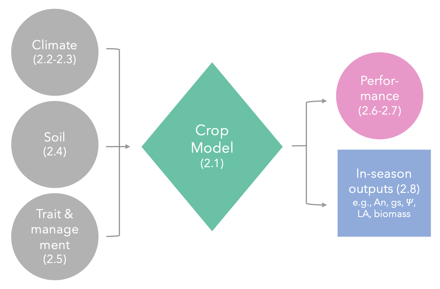
We set up a data-model framework to quantitatively identify high performing regions within a T $\times$ E $\times$ M landscape. The framework consists of three main components (Fig. 1): 1) a process-based crop simulation model (section 2.1), 2) model inputs to drive the model, including present-day climate information (section 2.2), idealized future climate information (section 2.3), simulation site soil information (section 2.4), and sampled trait and management options (section 2.5), and 3) processed model outputs that identify performance within the T $\times$ E $\times$ M landscape (section 2.6 - 2.7), and summarized in-season growth outputs (section 2.8).

Figure 1: Diagram of the data-model framework.

2.1 Process-based crop simulation model - MAIZSIM

MAIZSIM is a deterministic and dynamic model developed and calibrated for maize plants to represent key physiological and physical processes such as gas exchange, canopy radiative transfer, carbon partitioning, water relations, nitrogen dynamics and phenology [31]. MAIZSIM interfaces with a 2-dimensional finite element model (2DSOIL) that simulates a dynamic soil water and nutrient vertical 2D profile [59]. The coupled model responds to daily or hourly meteorological information throughout the growing season that includes temperature, relative humidity, solar radiation, and CO₂ concentrations.

At the leaf-level, MAIZSIM captures gas exchange processes through a C4 photosynthesis model [64] coupled with a stomatal conductance model [2] and an energy balance equation [9]; leaf-level gas exchange processes are scaled to canopy-levels using a sunlit/shaded leaf framework [13]. The model simulates crop development throughout the growing season following a nonlinear temperature response [69], and adopts a leaf area model developed by [34] to describe the expansion and senescence of individual leaves. MAIZSIM dynamically simulates leaf water potential and uses it to trigger water stress responses such as reduced growth rate and hastened senescence when values drop below designated thresholds [68].

The model has been validated at different scales – including physiological aspects such as gas exchange [67], leaf development and biomass gain [31], leaf growth water stress responses [68], as well as field-level validations in AgMIP projects [3, 32] and FACE site studies [17] that tested for yield responses to different temperature and CO₂ conditions. The model has also recently been used to test the independent impacts of temperature versus VPD on growth and yield in maize growing regions in the US [29].

Figure 2: Simulation sites and number of years simulated (purple triangles), along with historic maize yield and planting area data (green circles). Colors indicate yield and circle size indicate planting area.

2.2 Present-day climate data

We assembled hourly data of temperature, relative humidity, precipitation, and solar radiation over years 1961-2005 for our simulation sites as weather data input for our model simulations. Specifically, we accessed hourly air temperature ($T_{air}$), dew point temperature ($T_{dew}$), and precipitation data from the NOAA National Center for Environmental Information Integrated Surface Hourly database (https://www.ncdc.noaa.gov/isd), and hourly solar radiation data from the National Solar Radiation Data Base (https://nsrdb.nrel.gov/data-sets/archives.html).

We followed the Clausius-Clapeyron equation (Eqn. 1-2) to back out atmospheric humidity information in the form of relative humidity (RH) from $T_{air}$ and $T_{dew}$:

$$E_{s}=E_{sref}\cdot e^{\frac{L_{v}}{R_{v}}\cdot(\frac{1}{T_{ref}}-\frac{1}{T_{air}})}$$ (1)

$$E=E_{sref}\cdot e^{\frac{L_{v}}{R_{v}}\cdot(\frac{1}{T_{ref}}-\frac{1}{T_{dew}})}$$ (2)

The equation uses the saturation vapor pressure ($E_{sref}$, 6.11 mb) at a reference temperature ($T_{ref}$, 273.15 K), the vaporization latent heat ($L_{v}$, 2.5$\cdot$10⁶ J kg^-1), and the gas constant ($R_{v}$, 461 J K^-1kg^-1) to calculate the saturated water vapor pressure ($E_{s}$, mb) and the actual water vapor pressure ($E$, mb) at air temperature ($T_{air}$, K). We then use $E$ and $E_{s}$ to calculate $RH$ (%) (Eqn. 3):

$$RH=\frac{E}{E_{s}}$$ (3)

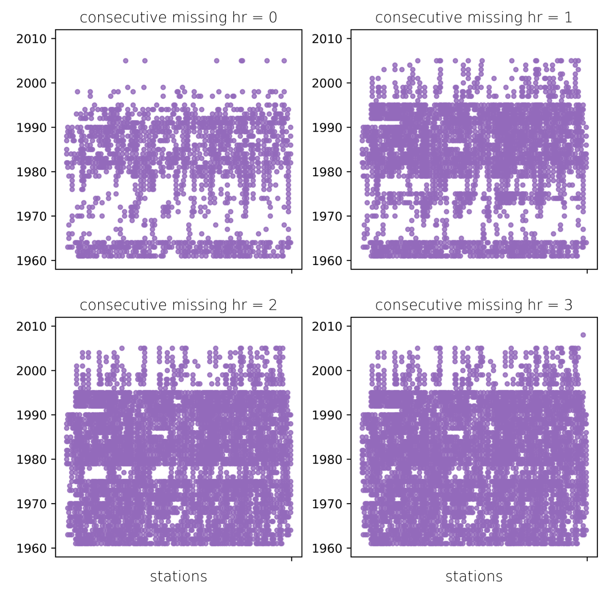
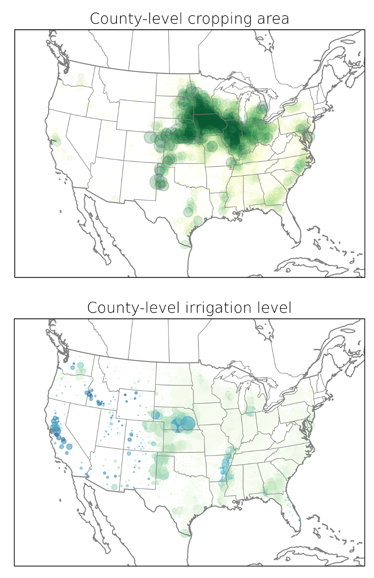
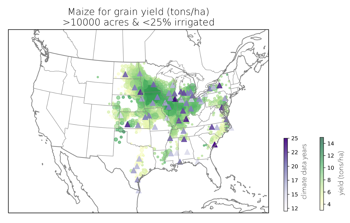
We selected overlapping sites and years that had data available from both the Integrated Surface Hourly Data Base and the National Solar Radiation Data Base over years 1961-2005 and filtered for site-years that had less than two consecutive hours of missing data throughout the growing season (broadly defined to be between February 1^st – November 30^th) and retained at least two-thirds of the weather data (Fig. S1). We then gap-filled any missing data by linearly interpolating the missing information with weather data of the hours prior and post the missing data point. Next, we linked valid weather stations with maize planting area and irrigation level data accessed through the United States Department of Agriculture – National Agriculture Statistics Service (USDA- NASS, https://www.nass.usda.gov/Data_and_Statistics/index.php). Specifically, we calculated the average maize planting area across our simulation period (1961-2005) in the continental US and accessed average irrigation level (%) for the same sites through four available census years (1997, 2002, 2007, 2012) (Fig. S2). We used the planting area and irrigation level averaged across five USDA-NASS sites closest to each weather station (via Euclidean distance) to represent their cropping information, and to exclude sites that either had less than 10,000 acres of corn planted or had greater than 25 % of crop land irrigated. We excluded sites with less than 15 years of data to insure sufficient sampling to assess inter-annual climate variability [55, 62]. Following this method, we were able to compile 1160 site-years of meteorology data for our simulations, which included a total of 60 sites, each site with available weather data ranging from 15-27 years (Fig. 2).

2.3 Idealized projected climate

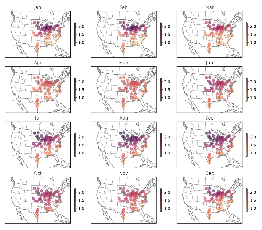
We assembled idealized projected climate information at two future time points, 2050 and 2100, to analyze crop performance shifts under future climate (Table 1). Specifically, we created monthly temperature and relative humidity anomaly maps under a substantial but not extreme greenhouse gas emissions scenario (SSP3-7.0, [50], Riahi2017) from the latest Coupled Model Intercomparison Project version 6 (CMIP6) outputs; we used these anomaly maps to calculate location-specific warming and associated changes in relative humidity levels throughout the growing season for each simulation site (Fig. 3). This method preserves correlations between climate variables (i.e., between temperature, relative humidity, and solar radiation) on short timescales and limits known biases in modeled variability [63, 16]. Since both magnitude and pattern of future precipitation projections are highly uncertain, we applied a general trend of precipitation reduction in accordance to the SSP3-7.0 scenario, and increased atmospheric concentrations of CO₂ to  550 ppm and  850 ppm for years 2050 and 2100, respectively [44].

Table 1: Description of idealized climate treatments with projected changes in temperature (T), relative humidity (RH), precipitation (precip.), and projected CO₂ concentrations by years 2050 and 2100 under the SSP3-7.0 emission scenario.

Year	Climate Scenario
2050	+ 1.4 °C mean T, -RH, -15% precip, 550 ppm
2100	+ 3.1 °C mean T, -RH, -30% precip, 850 ppm

Figure 3: Monthly pattern of warming derived from CMIP6 multimodel means for our simulation sites. Numbers in color bar indicate temperature scaling values to multiply with global average climate sensitivity to calculate projected warming for each simulation site. For example, under our assumption of 3.1°C global average warming by 2100, a scaling value of 2 for a specific simulation site will equal a total warming of 6.2°C for that location.

2.4 Soil data

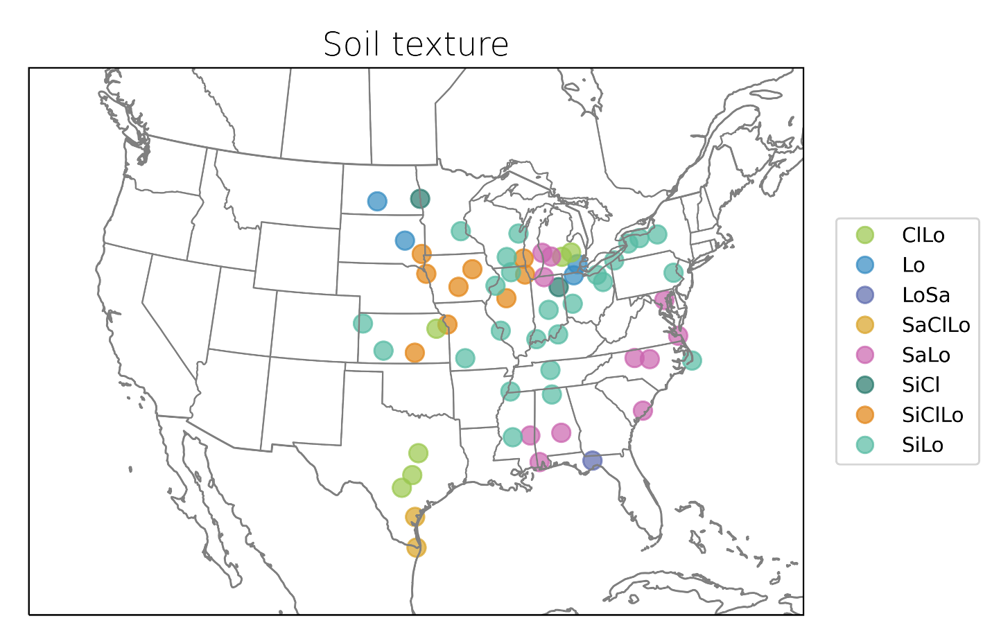
We used soil information from USDA-NASS locations nearby our simulation sites to curate site-specific soil files for each location. Soil properties are highly heterogeneous, and since our simulation sites are based on weather station locations that do not directly come from agricultural land, we use this method to broadly represent soil makeup of agricultural sites within the region without skewing towards any particular site. We queried soil information from the National Resources of Conservation Services (NRCS) SSURGO soil database [54] to identify soil properties for each NASS location with maize planting area greater than 10000 acres and irrigation levels less than 25%. For each site, we accessed soil information at five depth categories (surface, 50, 100, 150, and 200 cm), which included sand–silt–clay–organic matter composition, soil bulk density (the oven dry weight of less than 2 mm soil material per unit volume of soil at a water tension of 1/3 bar), and the volumetric content of soil water retained at a tension of 1/3 bar (33 kPa, field capacity) and 15 bar (1500 kPa, wilting point) expressed as a percentage of the whole soil. With the sand–silt–clay composition, we categorized the queried soil data into 12 texture groups following the USDA Textural Soil Classification [56] and excluded sites classified as Sandy or Clay due to their lack of representation in agricultural fields. Next, we determined the soil class within each depth category for all our simulation sites by assigning it the most prevalent soil class from it’s 11 nearest NASS sites calculated through Euclidean distance, and assigned it the mean soil conditions of that texture-depth class averaged across all NASS sites within that category. Finally, we estimated soil hydraulic properties of each soil type through a water release curve predicted by the van Genuchten equation [61].

Figure 4: Soil texture across simulation sites. Soil texture categories include clay loam (ClLo), loam (Lo), loamy sand (LoSa), sandy clay loam (SaLoLo), sandy loam (SaLo), silty clay (SiCl), silty clay loam (SiClLo), and silty loam (SiLo).

2.5 Sampling within the trait and management space

We selected several key model parameters that represent a range of maize traits and management options to investigate combinations that lead to high performance under present and future climate conditions. Since we do not have robust observation-based data on the natural distribution and boundaries of most parameters, we assumed a uniform distribution and set biologically reasonable boundaries around literature-based default values (Table 2). We assumed all parameters to be non-correlated and used a Latin hypercube sampling method [36] to create 100 different trait-management (T $\times$ M) combinations within the parameter space.

Table 2: MAIZSIM parameters tested for yield optimization

Processes	Params	Description	Default (Range)	Citation
Physiology	g1	Ball-Berry gs model slope	4 (2$\sim$6)	[41, 53]
	Vcmax	Max RUBISCO capacity	65 (65$\sim$80)	[30, 66]
	Jmax	Max electron transport rate	350 (350$\sim$420)	[30, 66]
	phyf	Reference leaf water potential (MPa) used to describe stomata sensitivity to leaf water potential	-1.9 (-3$\sim$-1)	[60, 67, 53]
Phenology	SG	Duration that leaves maintain active function (stay-green) after reaching maturity	3 (2$\sim$6)	[70, 24, 58]
	gleaf	Total leaf number	19 (11$\sim$25)	[46, 45]
	LTAR	Max leaf tip appearance rate (leaves/day)	0.5 (0.4$\sim$0.8)	[31, 45]
Morphology	LM	Leaf length of the longest leaf (cm)	115 (80$\sim$120)
	LAF	Leaf angle factor	1.37 (0.9$\sim$1.4)	[6, 19]
Management	gdd	Growing degree days accumulated by sowing	100 (80$\sim$160)	[52, 58]
	pop	Density (plants/m2)	8 (6$\sim$10)	[58, 57]

2.6 Performance within the T $\times$ E $\times$ M landscape

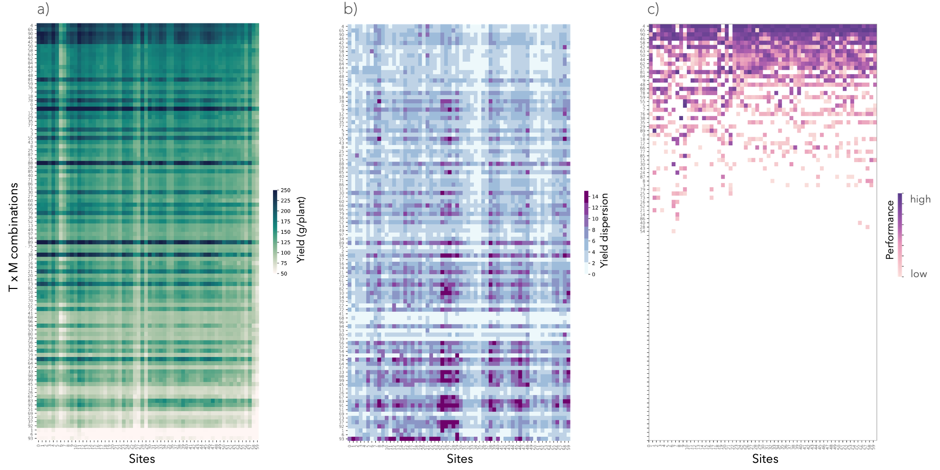
We defined high crop performance as crops that achieve high yield (i.e. yield mean across years) and high yield stability (i.e. yield dispersion across years). We developed a cost function (Eqn. 4) to quantify the performance of any T $\times$ M combination by calculating its distance to a theoretical best-performing combination within the yield and yield stability space (Eqn. 4):

$$D_{score}=\sqrt{w_{yield}*(y_{mean}-y_{max})^{2}+w_{disp}*(y_{disp}-d_{min})^{2}}$$ (4)

$y_{mean}$ and $y_{disp}$ represent mean yield and yield dispersion (variance/mean) across years for the target T $\times$ M combination at a specific simulation site, respectively. We standardized yield and dispersion to values between 0 and 1 to avoid skewed contribution due to difference in scale. $y_{max}$ and $d_{min}$ denote the standardized maximum mean yield (1) and minimum yield dispersion (i.e., maximum yield stability, 0) achieved within all T $\times$ M combinations at a specific simulation site. $w_{yield}$ and $w_{disp}$ are empirical coefficients between 0 and 1 that assign weighted importance to yield mean and yield dispersion, respectively.

We used the calculated $D_{score}$ to rank the top 20 performing T $\times$ M combinations for each simulation site. We determined an overall ranking for each T $\times$ M combination based on their rankings across all simulation sites (Fig. 5a). With this method, T $\times$ M combinations with high rankings across a few sites versus combinations with medium ranking across several sites can all result in overall high performance. T $\times$ M combinations that do not rank within the top 20 performers at any site will not receive a ranking.

Figure 5: Simulated a) yield, b) yield dispersion, and c) performance ranking of across T $\times$ M combinations and locations. T $\times$ M combinations are ordered from top to bottom starting from the highest performance ranking. Sites are order from left to right from sites located in the south to the north.

2.7 Regional difference in performance

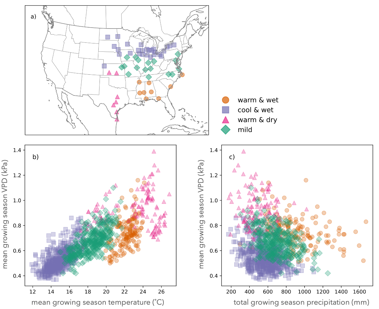
We used a climate space approach to identify how the performance of T $\times$ M combinations differed with baseline climate conditions. We used a k-means clustering algorithm to cluster our sites based on mean growing season temperature and VPD, and total growing season precipitation, roughly dividing our simulation sites into four groups of climate spaces - cool and medium precip, mild, warm and wet, and warm and mild to dry (Fig. 6). We analyzed the performance of T $\times$ M combinations within each cluster of sites by calculating a standardized performance score (Eqn. 5):

$$P_{score}=\frac{\sum_{i=1}^{n}R_{i}}{R_{max}*n}$$ (5)

$R_{i}$ denotes the performance ranking of a T $\times$ M combination at site $i$ among a total of $n$ sites within each climate space, and $R_{max}$ indicates the maximum performance ranking a T $\times$ M combination can achieve at a single site. In our workflow, we only considered the top 20 performing T $\times$ M combinations when ranking high performing combinations (see section 2.6), so $R_{max}$ equals 20. The resulting standardized performance score ranges between 0 and 1, in which a T $\times$ M combination that ranks with highest in performance across all locations within the climate space would receive a $P_{score}$ of 1.

Figure 6: a) Map of simulation sites clustered based on mean growing season temperature (°C), mean growing season VPD (kPa), and total growing season precipitation (mm). Mean growing season temperature (°C), mean growing season VPD (kPa), and total growing season precipitation (mm) levels for all simulated site-years (b, c).

2.8 In-season model outputs

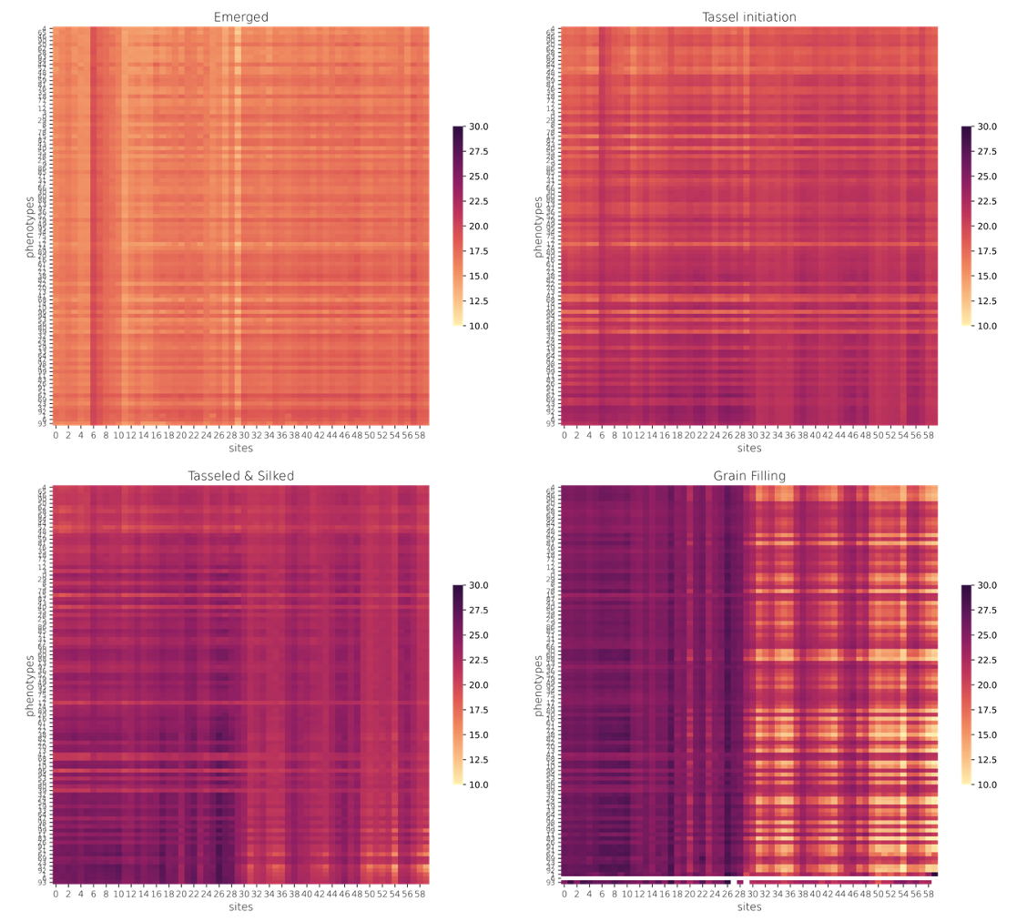
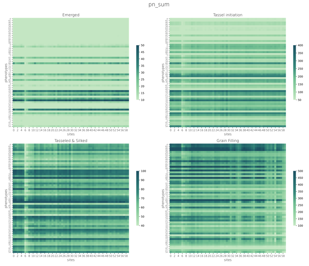
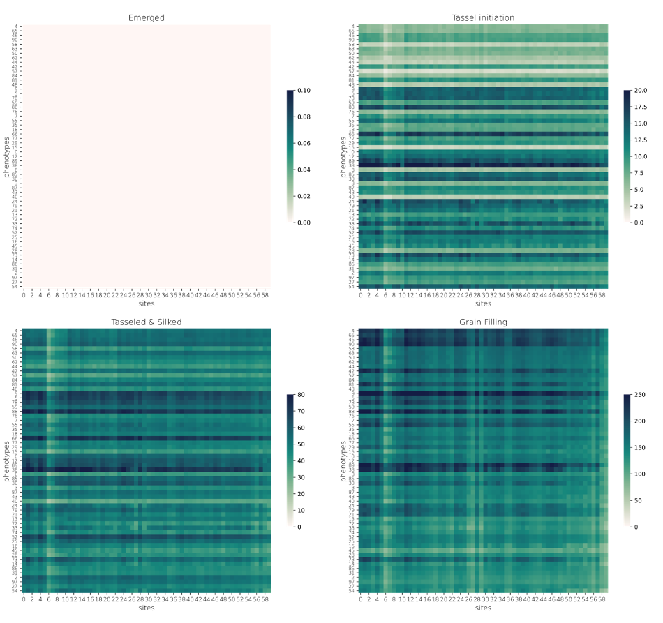
MAIZSIM generates outputs of a number of plant growth outputs throughout the growing season on an hourly time step. We describe in Table 3 a select few outputs in more detail. We summarized these high time frequency outputs across four phenological stages (emerged, tassel initiation, tasseled and silked, and grain-filling) to facilitate analysis and interpretation. Specifically, we queried net photosynthetic rate ($A\textsubscript{n}$), net carbon gain ($P\textsubscript{n}$), and stomatal conductance ($g\textsubscript{s}$) values from daylight hours, and averaged them within the designated phenological stages. We represented ear biomass, total biomass, and total leaf area ($ear\_biomass$, $total\_biomass$, $LA$) within each developmental stage with maximum values within each stage. Finally, we queried water supply, demand, and deficit ($ET\_supply$, $ET\_demand$, $water\_deficit$) values at noon and averaged all values within each phenological stage, and represented predawn leaf water potential ($\Psi$) with values queried at 5 am, and averaged the all values within each phenological stage.

Table 3: Key model outputs

Output	Description	Unit
$A_{n}$	Net photosynthetic rate	µmol CO2 m-2 sec-1
$P_{n}$	Net carbon gain	g /plant hour
$g_{s}$	Stomatal conductance	g H2O m-2 sec-1
$ear\_biomass$	Total ear biomass	g/plant
$total\_biomass$	Total plant biomass	g/plant
$LA$	Total leaf area	cm2
$phenostage$	Phenological stage	-
$ET\_supply$	Evapotranspiration (ET) supply	g H2O
$ET\_demand$	Evapotranspiration demand	g H2O
$water\_deficit$	ET demand - ET supply	g H2O
$\Psi$	Leaf water potential	MPa

2.9 Experiment setup and model simulation

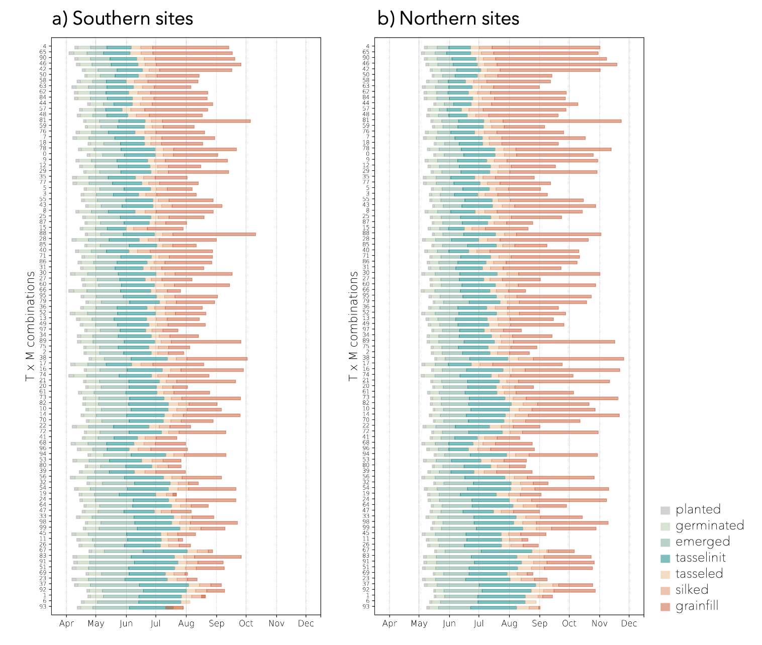
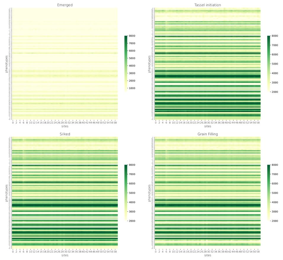
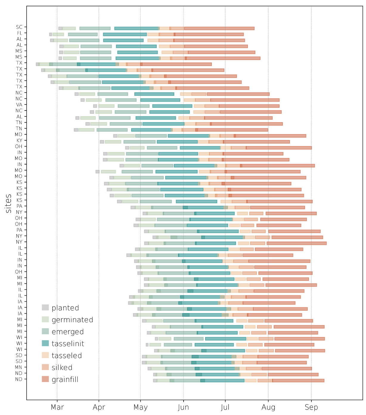
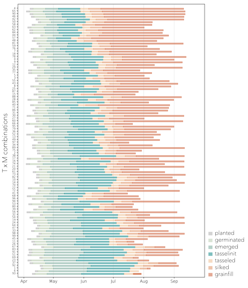
We prescribed the sampled planting density (Table 2, pop) for each ensemble member and adjusted the planting date for each ensemble member and simulation site based on climate and growing degree days (GDD) requirements. We calculated GDD for each simulation site through accumulated heat units starting from February 1st with a base temperature of 8°C [31] and determined the planting date once GDD surpassed the sampled for each ensemble member (Table 2, gdd). This led to earlier planting dates in warmer regions and vice versa (Fig. 7), and created diversity in cropping cycle start time among T $\times$ M combinations, mimicking early versus late-planting cultivars (Fig. 13). To simulate well-fertilized conditions, we prescribed a total of 200 kg ha^-1 of nitrogen throughout the growing season, applying half as base fertilizer prior to planting and the rest top-dressed one month post planting.

Figure 7: Start time and duration of each phenological stage across simulation sites, indicated by state abbreviations. Sites are roughly ranked by latitude, starting from southernmost sites towards the top.

For each simulation site, we ran the MAIZSIM model with default parameters that represented a generic crop cultivar across all locations (see default values in Table 2). Next, we carried out a site-level ensemble of simulations in which we used past meteorology data (see section 2.2) to each of the 100 trait-management parameter combinations (see section 2.5) for each of our 1160 site–years (see section 2.6) and identified top performing (high yield and yield stability) trait-management combinations. Finally, we repeated the site-specific trait and management ensemble of simulations with idealized future climate (see section 2.3) to understand how high performing trait and management combinations under current climate conditions fared under future climate.

2.10 Model validation

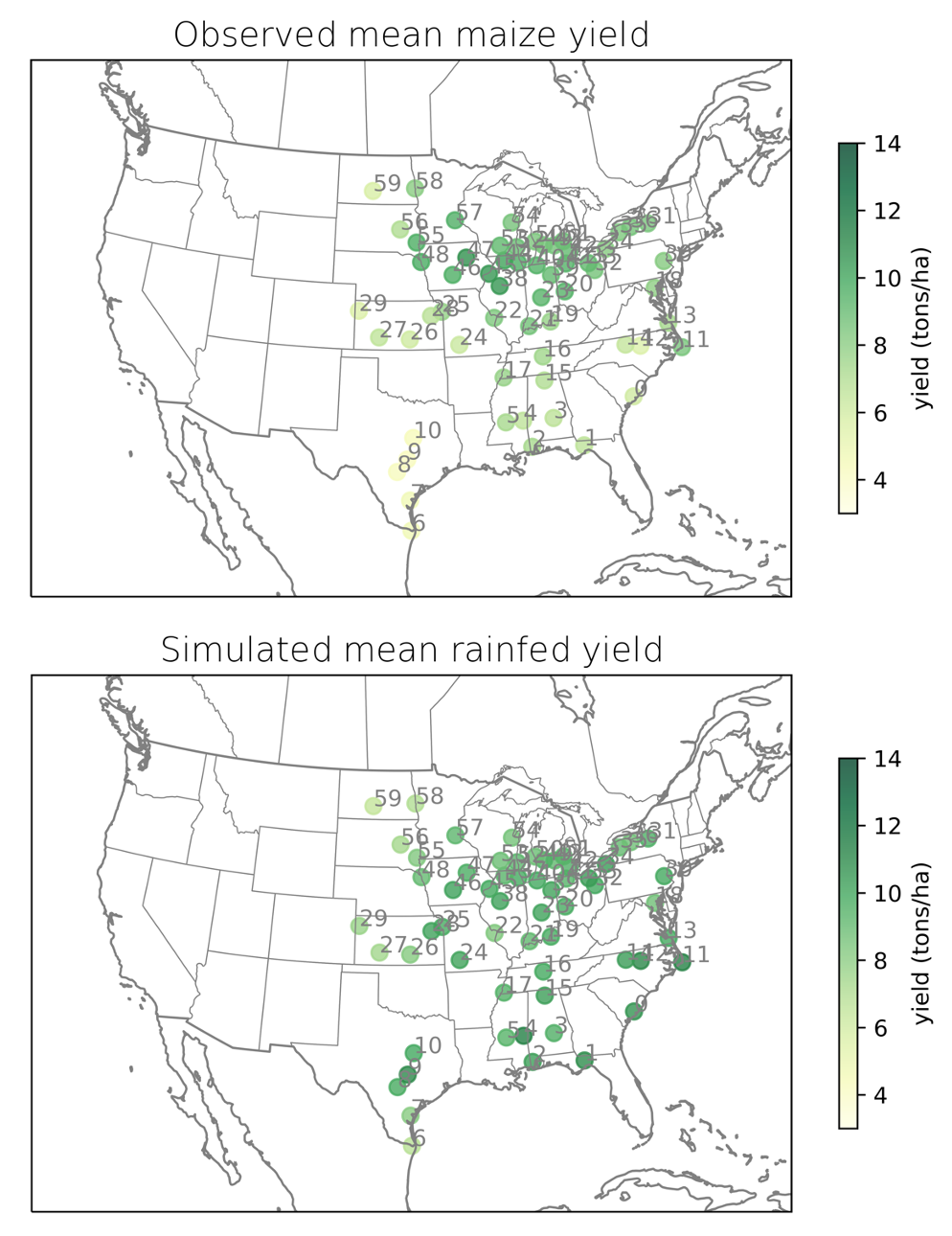
We validated simulated yields with default parameter values (control T $\times$ M combination, see Table 2) with historic yield data from the United States Department of Agriculture – National Agriculture Statistics Service (USDA- NASS, https://www.nass.usda.gov/Data_and_Statistics/index.php). We compared yield data from observation sites closest to our simulation sites calculated through a Euclidean distance (Fig. 8). We scaled our whole-plant level simulation outputs to field level by applying a planting density of 10 plants per m² and compared our simulated yield with averaged yield observations in between years 2005-2012, since our default parameter and management options resemble modern-day plant traits, planting density, and planting dates.

Figure 8: Observed (top) and simulated (bottom) yield (tons/ha) across simulated sites. Numbers indicate site numbers that correspond in Fig. 9.

3 Results and discussion

3.1 Model validation

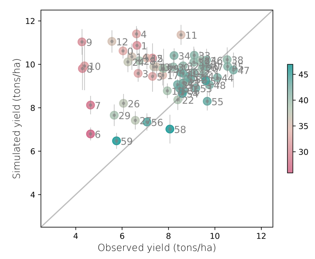
In general, simulated yields showed less spatial difference compared to observations (Fig. 8). The model captured historic yield observations well in the higher latitude Corn Belt regions but overestimated yield in various warmer sites in southern locations (Fig. 9). Southern locations experience much warmer temperatures, especially during later parts of the growing season (Fig. S3, grain-fill). While MAIZSIM dynamically describes temperature and water stress throughout the growing season through impacts on gas exchange and leaf developmental processes, the model lacks direct depiction of climate stress responses on reproduction processes such as flowering, pollination, and grain-filling, which are likely reasons for the yield over-estimation in warmer regions.

Cultivar differences between crops planted in southern versus northern locations could also contribute to these discrepancies. Farmers in warmer southern locations choose cultivars that are both planted and harvested earlier in the growing season, leading to an overall shorter crop cycle duration compared to those planted in the north (USDA-NASS, Crop Progress and Conditions). While our simulation set up captures earlier planting in warmer regions (Fig. 7), it does not capture potential differences in cultivar and management choices that growers in the south have likely been opting for in order to avoid late season heat and water stress. Finally, we note that by applying a universal soil depth (200 cm), we may be overestimating soil water availability. This could disproportionately affect warmer locations in south, in which late-season water availability could partially alleviate water stress later in the growing season and contribute to yield overestimation in those locations (Fig. 9).

Figure 9: Observed versus simulated yield (tons/ha) across simulated sites. Colors indicate latitude of simulation site. Numbers correspond to site numbers shown in Fig. 8.

3.2 Performance difference across climate spaces

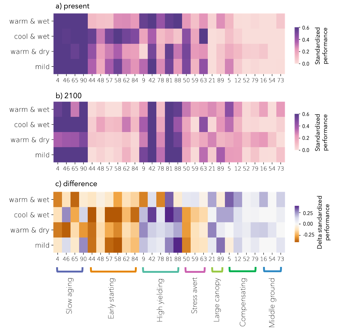
In [28] (Hsiao2022, submitted), we followed the framework described in this paper and identified several top-performing strategies among all T $\times$ M combinations under present-day and future climate conditions, categorized based on different combinations of phenological (grain-filling start time and duration) and morphological (total leaf area) features. Top-performing strategies under present-day climate conditions included T $\times$ M combinations that either reached reproductive stage early (Early Starting), were slow in aging (Slow Aging), stress averting (Stress Averting), or had large canopies and were high in yielding (High Yielding). More details are described in Hsiao et al. (2022) and briefly summarized below.

Early Starting, Slow Aging, and Stress Averting strategies all have a smaller canopy size and relatively earlier transition times from vegetative to reproductive stages, but differ in grain-filling duration. Slow Aging strategies have long grain-filling durations that prolong cropping duration, while Stress Averting strategies display the shortest longevity, allowing plants with this strategy to complete their cropping cycle early and avoid late season stressors such as dry and hot conditions. On the other hand, High Yielding strategies have larger canopy sizes accompanied by delayed transition from vegetative to reproductive stages. While all categorized as top-performing under present-day climate, these strategies showcase a range of trade-offs between yield and yield stability, with performance differing across simulation sites (Fig. 5, 10) and climate spaces (Fig. 11a).

Figure 10: Performance ranking across simulation sites for T $\times$ M combinations of different top-performing strategies under present-day climate conditions.

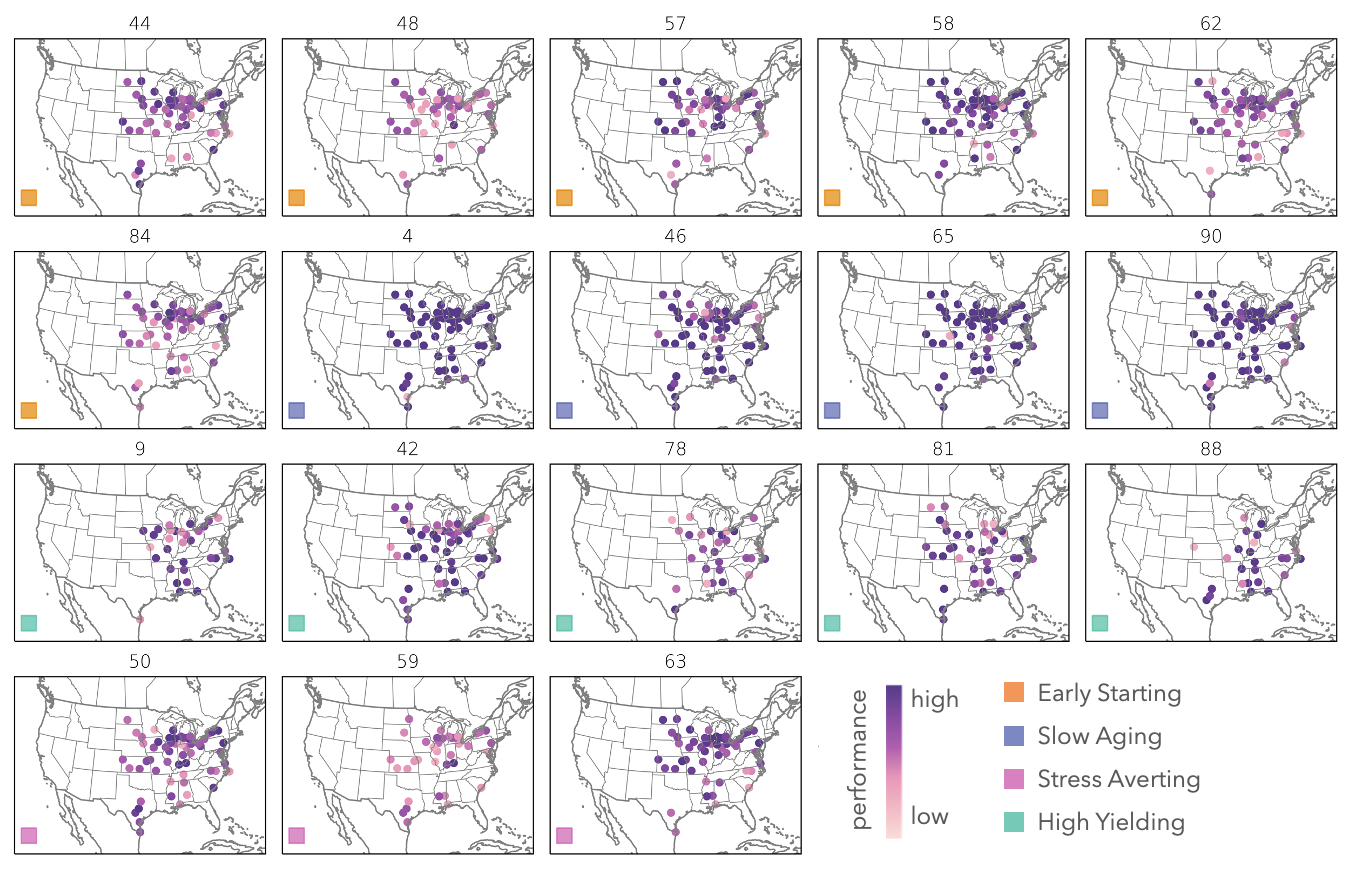
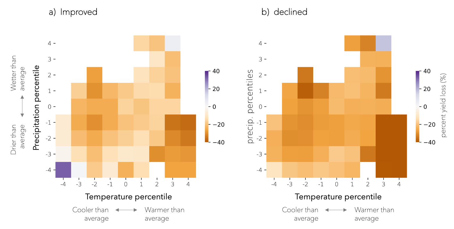
Under current climate conditions, T $\times$ M combinations with Slow Aging strategies tend to be generalists, showing high performance across all climate spaces. On the other hand, strategies such as Early Starting fared best in cool and wet regions, while High Yielding strategies perform best under warm and wet conditions (Fig. 11a). Under future climate conditions, we observed an overall yield loss for all T $\times$ M combinations in most simulation sites (Fig. 12), including strategies that improved in performance ranking with climate change (Fig. 12a), such as High Yielding and Large Canopy (Fig. 11c). In general, warmer regions with low precipitation levels exhibited the greatest yield sensitivity (% yield loss per degree C of warming, Fig. 12); high-performing strategies under future climate partially buffered, but did not prevent yield loss.

High-performing strategies under present-day climate conditions shifted with climate change (Fig. 11b, c). T $\times$ M combinations with early starting strategies experienced the greatest drop in performance ranking overall, showing declines in most climate spaces (Fig. 11c, Early Starting). Slow aging strategies still remained one of the higher performers by the end of the century (Fig. 11b, Slow Aging), but showed clear performance ranking declines in warm climate spaces (Fig. 11c, Slow Aging), allowing several other strategies to compete for top performance in those climate spaces (Fig. 11c); T $\times$ M combinations with high yielding and compensating strategies progressed further in performance ranking (Fig. 11c, High Yielding), and new high-performing strategies with larger canopies and delayed transition timings into reproductive stages emerged (Fig. 11c, Large Canopy, Compensating, Middle Ground).

Figure 11: Standardized performance rankings of different strategies across climate spaces (see section 2.7) under a) current, b) future climate conditions, and c) the difference between the two.

Figure 12: Percent yield loss within mean growing season temperature-precipitation climate space among T $\times$ M combinations that a) improved versus, b) declined in performance ranking under future climate conditions.

Figure 13: Start time and duration of each phenological stage across T $\times$ M combinations, averaged across all simulation sites, ranked by overall performance, with the highest performers listed towards the top.

Figure 14: Relationship between mean temperature (°C) and mean photosynthetic rate (µmol CO₂ m^-2 sec^-1) for all simulated site-years during a) vegetative versus b) reproductive stages for four representative T $\times$ M combinations within top-performing strategies.

3.3 Mechanisms for high performance

We analyzed detailed in-season outputs of various phenological, physiological, and morphological outputs of the model (Table 3) and describe here some general trends observed in top-performing T $\times$ M combinations.

3.3.1 Phenology

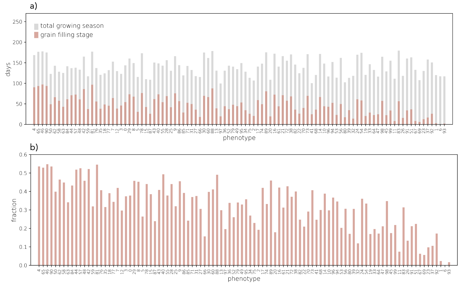
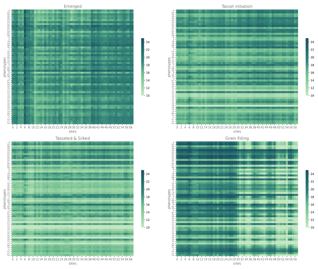
Climatological differences between simulation sites and parameter differences among T $\times$ M combinations both lead to the range of phenology output we see in our simulation outputs (Fig. 7, 13). Phenology differs across simulation sites due to imposed planting date adjustments based on growing degree day requirements, allowing for an earlier planting date in warmer regions (Fig. 7). Climatological differences throughout the growing season further shape the difference, especially during the grain-filling stage in which simulation sites in the south become substantially warmer than those in the north (Fig. S3), leading to hastened development (Fig. S5). On the other hand, phenology differs among T $\times$ M combinations due to differences in perturbed traits linked to phenology (e.g. planting time, developmental rate, leaf number, Fig. 13). High performing T $\times$ M combinations under present-day climate conditions tend to show earlier starts in reproductive stages with a longer duration (Fig. 13). Higher ranking T $\times$ M combinations tend to show a greater fraction of grain-filling length over total growing season length (Fig. S4b) despite no clear trends in total growing season length (Fig. S4a).

3.3.2 Physiology

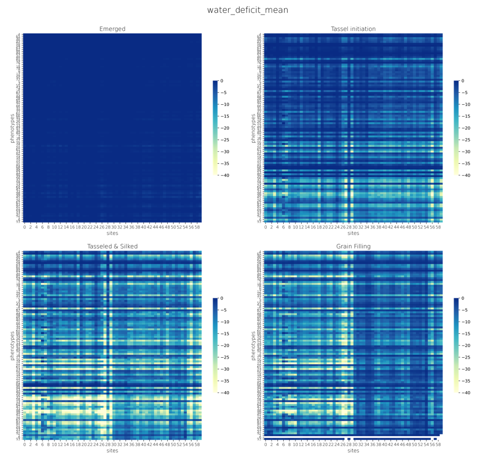
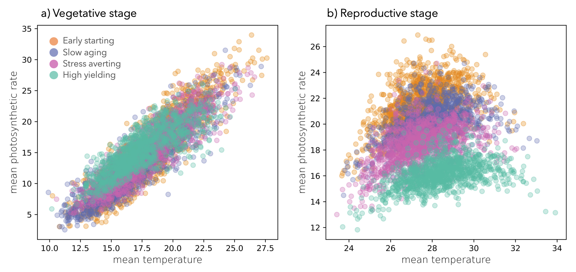
Net photosynthetic rates are generally higher in top-performing T $\times$ M combinations during transition from vegetative into reproductive stages (Fig. S6), but the differences in photosynthetic rates become dominated by climatological differences between simulation sites during the final grain-filling stage, with greater photosynthetic rates in warmer southern regions (Fig. S6). In general, we see a linear relationship between temperature and photosynthetic rate during vegetative stages (Fig. 14). This relationship eventually plateaus around 28-30 °C later in the growing season, and starts to decline in a few warmest site-years (Fig. 14b). While warmer temperatures generally led to higher photosynthetic rates, hastened development and greater water deficit under warmer conditions also led to overall shorter grain-filing durations (Fig. S7, S5a), compensating one another, dampening the overall difference between northern versus southern sites in terms of net carbon gained throughout grain-filling (Fig. S8) and final yield (Fig. S9).

3.3.3 Morphology

Differences in simulated total leaf area was largely dominated by parameter make up within T $\times$ M combinations, showing much less difference in simulated yield across sites (Fig. S10). Simulated plants approached full canopy sizes around tassel initiation, and top-performing combinations showed mid to lower total leaf area under present-day climate conditions. This was consistent with most top-performers under present-day climate exhibiting early transitions into reproductive stage (e.g., Slow Aging, Early Starting, Stress Averting). These strategies partly achieved early reproductive start through short vegetative stages through fewer total number of leaves and hence smaller canopy size (i.e., lower total leaf area).

4 Discussion

Crop production is expected to suffer under future climate conditions as the climate warms. Adaptation of crop management practices, location of planting, as well as adaptation of the crops themselves all have the potential to limit expected yield loss and help to sustain agricultural productivity. However, we lack a systematic understanding of which adaptations are likely to have the biggest impact and why, both critical pieces of knowledge for agricultural planning. Mechanistic, process-based crop simulation models can be a powerful tool to synthesize cropping information, set breeding targets, and develop adaptation strategies for sustaining food production, yet have been underutilized for developing specific climate-adaptation options.

Breeding for and adopting new cultivars involve exploring and navigating the hills and valleys of the G $\times$ E $\times$ M landscape, in which optimal plant traits and management options are identified within defined target environments [39, 12]. Requirements from breeding, delivering, and adopting a desirable cultivar depends on many factors, and the whole process can take from years to decades [8]. Recent developments in breeding practices have greatly expanded the efficiency in genotyping and phenotyping methods [65], yet the breeding pipeline is still time and resource intensive, limiting its ability to explore the full range of G $\times$ E $\times$ M combinations and interactions.

A typical breeding cycle starts out by exposing a large germplasm pool under extremely high selection pressure, filtering genotypes from the order of 10⁶ individuals down to a few dozen promising candidates [37, 10]. In the early stages of a breeding program, trait selection is often limited to those that can easily be identified through automated processes, and commonly based on plants in early developmental stages. It is not until later in the breeding cycle that selection criteria shift from genotype to phenotype-based, and promising hybrids are evaluated on-farm at various locations with a range of background climate conditions [22]. Management optimization also occurs around this time, in which field trials are set up to identify the best management practices for the final candidates prior to commercial release. Further, common breeding methods that either select for higher yield or eliminate defect traits do not allow for a clear understanding of the mechanisms in which favorable traits contribute to greater performance and yield, and effective combinations of plant traits, if not actively sought for based on a mechanistic understanding of crop growth and yield, could only occur by chance [15].

There is growing recognition that mechanistic crop simulation models can be a powerful tool to synthesize cropping information, set breeding targets, and develop adaptation strategies for sustaining food production. Such applications can complement current breeding efforts of developing new climate-resilient cultivars by facilitating broad exploration of the G $\times$ E $\times$ M landscape within a modeled setting as a first step [43, 51, 11, 38]. The process-based nature of such models allow for mechanistic insight through which these adaptations influence yield and their sensitivity to different climate factors, providing a more complete assessment of the uncertainty associated with different possible climate conditions, including those that do not currently exist yet.

[49] (Ramirez-Villegas2015) provided a few successful examples of model-aided breeding projects, such as the New Plant Type program developed by IRRI for rice crops, in which process-based models were used to help make informed decisions to target breeding directions and resulted in new plant types that out-yielded conventional cultivars within two breeding cycles [48]. This success further inspired the super rice program in China that led to newly developed rice varieties with 15-25% higher yield than common hybrid cultivars planted in other regions in China [48]. While model-aided breeding practices are less commonly targeted towards a changing climate [49], demonstrated success under current climate suggest it as a promising pathway to guide breeding direction for climate adaptation moving forward, and expanded experiments evaluating a range of G $\times$ E $\times$ M conditions can enable production system responses to changing environmental conditions (Messina et al., 2020, Wang et al., 2019).

Regardless, thorough evaluation and application of crop models for developing specific climate-adaptation options (e.g., designing adaptive phenotypes for specific soil-climate combinations) for US agriculture remains scarce. We bridge this gap by constructing an integrated data-model framework set up to explore crop performance across a defined G $\times$ E $\times$ M landscape. With this framework, we identified high-performing plant trait and management combinations (G $\times$ M) best suited for current climate conditions, as well as targets and priorities to adapt to impending climate stressors (E). Heterogeneity in performance exists within the sampled climate space, which stemmed from underlying physiological, morphological, and phenological processes within the simulated crop. Model outputs on hourly time steps allowed us to compile detailed in-season outputs of various plant processes and summarize them according to associated phenological stages. This form of model output allows for more in-depth analysis that go beyond final yield and yield stability, and investigation of mechanisms that contribute to high crop performance and the differences across climate spaces and under future climate projections.

We demonstrate how such a framework can be used to identify adaptation options with an emphasis on climate-resilient plant traits and effective management that will mitigate yield loss and optimize productivity both across space and through time in US corn growing regions under future climate conditions. Our modeling results demonstrate that application of mechanistic modeling holds substantial promise to inform breeding within the US maize production system.

5 Acknowledgements

We thank Lucas Vargas Zeppetello for providing CMIP6 temperature and relative humidity projection scaling patterns. JH acknowledges support from the AFRI NIFA Fellowships Grant Program: Predoctoral Fellowships [grant no. 2020-67034-31736] from the USDA National Institute of Food and Agriculture. ALSS acknowledges support from NSF AGS-1553715.

6 Supplementary information

Figure S1: Available weather data based on different gap-filling intervals. For example, if consecutive missing hours equals 0, then only site-years with complete hourly weather data records will be included for weather data. If consecutive missing hour equals 1, site-years with gaps no greater than one hour consecutively will be included and gap-filled linearly.

Figure S2: Maize planting area (top) and irrigation levels (bottom) across continental U.S.

Figure S3: Mean air temperature (°C) across phenological stages for top phenotypes across all sites, ranked by performance of T $\times$ M combinations, and averaged within phenological stages.

Figure S4: a) Total growing season length (gray, days) and grain-filling length (pink, days) for all phenotypes, ranked by performance, starting with the highest performers towards the left, and b) the fraction of grain-filling over total growing season.

Figure S5: Start time and duration of each phenological stage across T $\times$ M combinations, averaged across all simulation sites for a) southern sites versus b) northern sites, ranked by overall performance, with the highest performers listed towards the top.

Figure S6: Net photosynthetic rate (µmol CO₂ m^-2 sec^-1) across phenotypes and sites, ranked by the performance of T $\times$ M combinations, and averaged within each developmental stage.

Figure S7: Mean water deficit (g H₂O) across phenotypes and sites, ranked by the performance of T $\times$ M combinations, and averaged within each developmental stage.

Figure S8: Net carbon gain throughout phenological stage (g C) across phenotypes and sites, ranked by the performance of T $\times$ M combinations, and averaged within each developmental stage.

Figure S9: Ear biomass (g/plant) across phenotypes and sites, ranked by the performance of T $\times$ M combinations, and averaged within each developmental stage.

Figure S10: Total leaf area (cm²) across phenotypes and sites, ranked by the performance of T $\times$ M combinations, and averaged within phenological stages..

References

- [1] D Andrivon et al. “Defining and designing plant architectural ideotypes to control epidemics ?” In Eur J Plant Patol, 2012 DOI: 10.1007/s10658-012-0126-y
- [2] J T Ball, I E Woodrow and J A Berry “A model predicting stomatal conductance and its contribution to the control of photosynthesis under different environmental conditions” In Progress in photosynthesis research 4.5, 1987, pp. 221–224 DOI: 10.1007/978-94-017-0519-6˙48
- [3] Simona Bassu et al. “How do various maize crop models vary in their responses to climate change factors?” In Global Change Biology 20.7, 2014, pp. 2301–2320
- [4] Marshall B Burke, David B Lobell and Luigi Guarino “Shifts in African crop climates by 2050 , and the implications for crop improvement and genetic resources conservation” In Global Environmetnal Change 19, 2009, pp. 317–325 DOI: 10.1016/j.gloenvcha.2009.04.003
- [5] Ethan E. Butler, Nathaniel D. Mueller and Peter Huybers “Peculiarly pleasant weather for US maize” In Proceedings of the National Academy of Sciences of the United States of America 115.47, 2018, pp. 11935–11940 DOI: 10.1073/pnas.1808035115
- [6] G S Campbell “Extinction coefficients for radiation in plant canopies calculated using an ellipsoidal inclination angle distribution” In Agricultural and Forest Meteorology 36, 1986, pp. 317
- [7] V.. Cardwell “Fifty Years of Minnesota Corn Production: Sources of Yield Increase1” In Agronomy Journal 74.6, 1982, pp. 984 DOI: 10.2134/agronj1982.00021962007400060013x
- [8] Andrew J. Challinor et al. “Improving the use of crop models for risk assessment and climate change adaptation” In Agricultural Systems 159, 2017, pp. 296–306 DOI: 10.1016/j.agsy.2017.07.010
- [9] G J Collatz, M Ribas-Carbo and J A Berry “Coupled Photosynthesis-Stomatal Conductance Model for Leaves of C4 Plants” In Australian Journal of Plant Physiology 19.5, 1992, pp. 519–538 DOI: 10.1071/PP9920519
- [10] Mark Cooper et al. “Predicting the future of plant breeding: Complementing empirical evaluation with genetic prediction” In Crop and Pasture Science 65.4, 2014, pp. 311–336 DOI: 10.1071/CP14007
- [11] Mark Cooper et al. “Integrating genetic gain and gap analysis to predict improvements in crop productivity” In Crop Science 60.2, 2020, pp. 582–604 DOI: 10.1002/csc2.20109
- [12] Mark Cooper et al. “Use of crop growth models with whole-genome prediction: Application to a maize multienvironment trial” In Crop Science 56.5, 2016, pp. 2141–2156 DOI: 10.2135/cropsci2015.08.0512
- [13] D G G Pury and G D Farquhar “Simple scaling of photosynthesis from leaves to canopies without the errors of big-leaf models” In Plant, Cell & Environment 20, 1997, pp. 537–557
- [14] D. Deryng, W.. Sacks, C.. Barford and N. Ramankutty “Simulating the effects of climate and agricultural management practices on global crop yield” In Global Biogeochemical Cycles 25.2, 2011 DOI: 10.1029/2009gb003765
- [15] C.. Donald “The breeding of crop ideotypes” In Euphytica 17, 1968, pp. 385–403
- [16] M.. Donat, A.. Pitman and S.. Seneviratne “Regional warming of hot extremes accelerated by surface energy fluxes” In Geophysical Research Letters 44.13, 2017, pp. 7011–7019 DOI: 10.1002/2017GL073733
- [17] Jean-Louis Durand et al. “How accurately do maize crop models simulate the interactions of atmospheric CO2 concentration levels with limited water supply on water use and yield?” In Eur J Agron 100, 2018, pp. 67–75
- [18] Donald N. Duvick “The Contribution of Breeding to Yield Advances in maize (Zea mays L.)” In Advances in Agronomy 86, 2005, pp. 83–145 DOI: 10.1016/S0065-2113(05)86002-X
- [19] Matthew J. Dzievit, Xianran Li and Jianming Yu “Dissection of Leaf Angle Variation in Maize through Genetic Mapping and Meta‐Analysis” In The Plant Genome 12.1, 2019, pp. 180024 DOI: 10.3835/plantgenome2018.05.0024
- [20] R.. Fischer and Gregory O. Edmeades “Breeding and cereal yield progress” In Crop Science 50, 2010, pp. S–85–S–98 DOI: 10.2135/cropsci2009.10.0564
- [21] Ana Fita et al. “Breeding and domesticating crops adapted to drought and salinity: A new paradigm for increasing food production” In Frontiers in Plant Science 6, 2015, pp. 1–14 DOI: 10.3389/fpls.2015.00978
- [22] Jim Gaffney et al. “Industry-scale evaluation of maize hybrids selected for increased yield in drought-stress conditions of the US corn belt” In Crop Science 55.4, 2015, pp. 1608–1618 DOI: 10.2135/cropsci2014.09.0654
- [23] H Charles J Godfray et al. “Food Security: The Challenge of Feeding 9 Billion People” In Science 327.5967, 2010, pp. 812–818 DOI: 10.1126/science.1185383
- [24] Per L. Gregersen, Andrea Culetic, Luca Boschian and Karin Krupinska “Plant senescence and crop productivity” In Plant Molecular Biology 82.6, 2013, pp. 603–622 DOI: 10.1007/s11103-013-0013-8
- [25] G.L. Hammer et al. “Designing crops for adaptation to the drought and high temperature risks anticipated in future climates” In Crop Science, 2020, pp. 1–17 DOI: 10.1002/csc2.20110
- [26] Graeme L. Hammer et al. “Can changes in canopy and/or root system architecture explain historical maize yield trends in the U.S. corn belt?” In Crop Science 49.1, 2009, pp. 299–312 DOI: 10.2135/cropsci2008.03.0152
- [27] Jerry L Hatfield and Charles L Walthall “Meeting Global Food Needs : Realizing the Potential via Genetics × Environment × Management Interactions”, 2015, pp. 1215–1226 DOI: 10.2134/agronj15.0076
- [28] Jennifer Hsiao et al. “Model-aided climate adaptation for future maize in the U.S.” In submitted, 2022
- [29] Jennifer Hsiao, Abigail… Swann and Soo-Hyung Kim “Maize yield under a changing climate: The hidden role of vapor pressure deficit” In Agricultural and Forest Meteorology 279 Elsevier, 2019, pp. 107692 DOI: 10.1016/j.agrformet.2019.107692
- [30] Soo-Hyung Kim et al. “Canopy photosynthesis, evapotranspiration, leaf nitrogen, and transcription profiles of maize in response to CO2 enrichment” In Global Change Biology 12.3, 2006, pp. 588–600 DOI: 10.1111/j.1365-2486.2006.01110.x
- [31] Soo-Hyung Kim et al. “Modeling temperature responses of leaf growth, development, and biomass in maize with MAIZSIM” In Agronomy Journal 104.6, 2012, pp. 1523–1537 DOI: 10.2134/agronj2011.0321
- [32] Bruce A. Kimball et al. “Simulation of maize evapotranspiration: An inter-comparison among 29 maize models” In Agricultural and Forest Meteorology 271 Elsevier, 2019, pp. 264–284 DOI: 10.1016/j.agrformet.2019.02.037
- [33] Christopher J. Kucharik “Contribution of planting date trends to increased maize yields in the central United States” In Agronomy Journal 100.2, 2008, pp. 328–336 DOI: 10.2134/agronj2007.0145
- [34] J.. Lizaso, W.. Batchelor and M.. Westgate “A leaf area model to simulate cultivar-specific expansion and senescence of maize leaves” In Field Crops Research 80.1, 2003, pp. 1–17 DOI: 10.1016/S0378-4290(02)00151-X
- [35] Susan McCouch et al. “Feeding the future” In Nature 499.7456, 2013, pp. 23–24 DOI: 10.1038/499023a
- [36] M.. McKay, R.. Beckman and W.. Conover “A comparison of three methods for selecting values of input variables in the analysis of output from a computer code” In Technometrics 21.2, 1979, pp. 239–245 DOI: 10.1080/00401706.2000.10485979
- [37] Carlos D. Messina et al. “Two decades of creating drought tolerant maize and underpinning prediction technologies in the US corn-belt: Review and perspectives on the future of crop design” In bioRxiv, 2020 DOI: 10.1101/2020.10.29.361337
- [38] Carlos D. Messina, Mark Cooper, Matthew Reynolds and Graeme L. Hammer “Crop science: A foundation for advancing predictive agriculture” In Crop Science 60.2, 2020, pp. 544–546 DOI: 10.1002/csc2.20116
- [39] Carlos D. Messina et al. “Yield-trait performance landscapes: From theory to application in breeding maize for drought tolerance” In Journal of Experimental Botany 62.3, 2011, pp. 855–868 DOI: 10.1093/jxb/erq329
- [40] Carlos D. Messina et al. “Limited-transpiration trait may increase maize drought tolerance in the US corn belt” In Agronomy Journal 107.6, 2015, pp. 1978–1986 DOI: 10.2134/agronj15.0016
- [41] Grace L. Miner, William L. Bauerle and Dennis D. Baldocchi “Estimating the sensitivity of stomatal conductance to photosynthesis: a review” In Plant Cell and Environment 40.7, 2017, pp. 1214–1238 DOI: 10.1111/pce.12871
- [42] N D Mueller, E E Butler, K A McKinnon and A Rhines “Cooling of US Midwest summer temperature extremes from cropland intensification” In Nature Climate Change 6.3, 2016 DOI: 10.1038/nclimate2825
- [43] Bertrand Muller and Pierre Martre “Plant and crop simulation models: Powerful tools to link physiology, genetics, and phenomics” In Journal of Experimental Botany 70.9, 2019, pp. 2339–2344 DOI: 10.1093/jxb/erz175
- [44] Brian C. O’Neill et al. “The Scenario Model Intercomparison Project (ScenarioMIP) for CMIP6” In Geoscientific Model Development 9.9, 2016, pp. 3461–3482 DOI: 10.5194/gmd-9-3461-2016
- [45] J.. Padilla and M.. Otegui “Co-ordination between leaf initiation and leaf appearance in field-grown maize (Zea mays): Genotypic differences in response of rates to temperature” In Annals of Botany 96.6, 2005, pp. 997–1007 DOI: 10.1093/aob/mci251
- [46] Boris Parent et al. “Maize yields over Europe may increase in spite of climate change, with an appropriate use of the genetic variability of flowering time” In Proceedings of the National Academy of Sciences of the United States of America 115.42, 2018, pp. 10642–10647 DOI: 10.1073/pnas.1720716115
- [47] Bin Peng et al. “Towards a multiscale crop modeling framework for climate change adaptation assessment” In Nature Plants 6.April Springer US, 2020 DOI: 10.1038/s41477-020-0625-3
- [48] Shaobing Peng et al. “Progress in ideotype breeding to increase rice yield potential” In Field Crops Research 108.1, 2008, pp. 32–38 DOI: 10.1016/j.fcr.2008.04.001
- [49] Julian Ramirez-Villegas, James Watson and Andrew J. Challinor “Identifying traits for genotypic adaptation using crop models” In Journal of Experimental Botany 66.12, 2015, pp. 3451–3462 DOI: 10.1093/jxb/erv014
- [50] Keywan Riahi et al. “The Shared Socioeconomic Pathways and their energy, land use, and greenhouse gas emissions implications: An overview” In Global Environmental Change 42, 2017, pp. 153–168 DOI: 10.1016/j.gloenvcha.2016.05.009
- [51] R.. Rötter, F. Tao, J.. Höhn and T. Palosuo “Use of crop simulation modelling to aid ideotype design of future cereal cultivars” In Journal of Experimental Botany 66.12, 2015, pp. 3463–3476 DOI: 10.1093/jxb/erv098
- [52] William J Sacks and Christopher J Kucharik “Crop management and phenology trends in the U.S. Corn Belt: Impacts on yields, evapotranspiration and energy balance” In Agric. For. Meteorol 151.7, 2011, pp. 882–894 DOI: 10.1016/j.agrformet.2011.02.010
- [53] Avat Shekoofa, Thomas R. Sinclair, Carlos D. Messina and Mark Cooper “Variation among maize hybrids in response to high vapor pressure deficit at high temperatures” In Crop Science 56.1, 2016, pp. 392–396 DOI: 10.2135/cropsci2015.02.0134
- [54] United States Department Agriculture. Soil Survey Staff “Soil Survey Geographic (SSURGO) Database.” Available online. Accessed [09/15/2019].
- [55] Afshin Soltani and Gerrit Hoogenboom “Minimum data requirements for parameter estimation of stochastic weather generators” In Climate Research 25.2, 2003, pp. 109–119 DOI: 10.3354/cr025109
- [56] Soil Survey Staff “Soil taxonomy: A basic system of soil classification for making and interpreting soil surveys. 2nd edition. Natural Resources Conservation Service. U.S. Department of Agriculture Handbook 436.”, 1999
- [57] P J Stone, A J Pearson, I B Sorensen and B T Rogers “Effect of row spacing and plant population on maize yield and quality” In Agronomy New Zealand 30, 2000, pp. 67–75
- [58] Dennis Timlin et al. “Chapter 3 - Maize water use and yield in the solar corridor system: a simulation study” In The Solar Corridor Crop System Academic Press, 2019, pp. 57–78 DOI: https://doi.org/10.1016/B978-0-12-814792-4.00003-6
- [59] Dennis Timlin, Yakov A. Pachepsky and Basil Acock “A design for a modular, generic soil simulator to interface with plant models” In Agronomy Journal 88.2 American Society of Agronomy, 1996, pp. 162–169 DOI: 10.2134/agronj1996.00021962008800020008x
- [60] A Tuzet, A Perrier and R Leuning “A coupled model of stomatal conductance, photosynthesis and transpiration” In Plant, Cell & Environment 26.7, 2003, pp. 1097–1116
- [61] M.. van Genuchten “A Closed-form Equation for Predicting the Hydraulic Conductivity of Unsaturated Soils” In Soil Science Society of America Journal 44.5, 1980, pp. 892–898 DOI: https://doi.org/10.2136/sssaj1980.03615995004400050002x
- [62] Justin Van Wart, Patricio Grassini and Kenneth G. Cassman “Impact of derived global weather data on simulated crop yields” In Global Change Biology 19.12, 2013, pp. 3822–3834 DOI: 10.1111/gcb.12302
- [63] Lucas R. Vargas Zeppetello, David S. Battisti and Marcia B. Baker “The origin of soil moisture evaporation “regimes”” In Journal of Climate 32.20, 2019, pp. 6939–6960 DOI: 10.1175/JCLI-D-19-0209.1
- [64] Susanne Caemmerer “Biochemical Models of Leaf Photosynthesis” Collingwood, Victoria, Australia: CSIRO Publishing, 2000, pp. 1–165
- [65] Kai P. Voss-Fels, Andreas Stahl and Lee T. Hickey “Q&A: Modern crop breeding for future food security 07 Agricultural and Veterinary Sciences 0703 Crop and Pasture Production 06 Biological Sciences 0607 Plant Biology 06 Biological Sciences 0604 Genetics” In BMC Biology 17.1 BMC Biology, 2019, pp. 1–7
- [66] Alex Wu et al. “Quantifying impacts of enhancing photosynthesis on crop yield” In Nature plants 5.4 Springer US, 2019, pp. 380–388 DOI: 10.1038/s41477-019-0398-8
- [67] Y Yang et al. “Simulating canopy transpiration and photosynthesis of corn plants under contrasting water regimes using a coupled model” In Transactions of the ASABE 52.3 American Society of AgriculturalBiological Engineers, 2009, pp. 1011–1024 DOI: 10.13031/2013.27370
- [68] Y Yang et al. “Simulating leaf area of corn plants at contrasting water status” In Agricultural and Forest Meteorology 149.6-7, 2009, pp. 1161–1167 DOI: 10.1016/j.agrformet.2009.02.005
- [69] Xinyou Yin, Martin J. Kropff, Graham McLaren and Romeo M. Visperas “A nonlinear model for crop development as a function of temperature” In Agricultural and Forest Meteorology 77.1-2, 1995, pp. 1–16 DOI: 10.1016/0168-1923(95)02236-Q
- [70] Jun Zhang et al. “Identification and characterization of a novel stay-green QTL that increases yield in maize” In Plant Biotechnology Journal 17.12 Blackwell Publishing Ltd, 2019, pp. 2272–2285 DOI: 10.1111/pbi.13139
- [71] Peng Zhu et al. “The important but weakening maize yield benefit of grain filling prolongation in the US Midwest”, 2018, pp. 4718–4730 DOI: 10.1111/gcb.14356