Instance-Dependent Label-Noise Learning with Manifold-Regularized Transition Matrix Estimation

Abstract

In label-noise learning, estimating the transition matrix has attracted more and more attention as the matrix plays an important role in building statistically consistent classifiers. However, it is very challenging to estimate the transition matrix $T(\textbf{x})$, where x denotes the instance, because it is unidentifiable under the instance-dependent noise (IDN). To address this problem, we have noticed that, there are psychological and physiological evidences showing that we humans are more likely to annotate instances of similar appearances to the same classes, and thus poor-quality or ambiguous instances of similar appearances are easier to be mislabeled to the correlated or same noisy classes. Therefore, we propose assumption on the geometry of $T(\textbf{x})$ that “the closer two instances are, the more similar their corresponding transition matrices should be”. More specifically, we formulate above assumption into the manifold embedding, to effectively reduce the degree of freedom of $T(\textbf{x})$ and make it stably estimable in practice. The proposed manifold-regularized technique works by directly reducing the estimation error without hurting the approximation error about the estimation problem of $T(\textbf{x})$. Experimental evaluations on four synthetic and two real-world datasets demonstrate that our method is superior to state-of-the-art approaches for label-noise learning under the challenging IDN.

1 Introduction

Label-noise learning has drawn more and more attention in the deep learning community, e.g.,[3, 53, 5, 50, 29, 11]. The main reason is that accurately annotating large-scale datasets becomes extremely costly and sometimes even infeasible [14]. An effective way is to collect such large-scale datasets from the crowd-sourcing platform [49] or online queries [4], which inevitably yield low-quality and noisy data. Thus, mitigating the side-effects of noisy labels becomes a very crucial topic. The noise model can be categorized as the class-conditional noise (CCN) and the instance-dependent noise (IDN). In CCN, each instance from one class has a fixed probability of being assigned to another. While in IDN, the probability that an instance is mislabeled depends on both its class and features. In this paper, we focus on the more promising IDN approach, which considers a more general noise and can cope with real-world noise.

The traditional label-noise learning methods can be divided into two categories: algorithms with statistically inconsistent classifiers and algorithms with statistically consistent classifiers. In the first category, algorithms do not model the label noise distribution explicitly, they usually employ some heuristics to reduce the negative effects of the label noise [8, 10, 11, 9]. Although such approaches often empirically work well, the learned classifier from the data with label noise may not be statistically consistent and their reliability cannot be guaranteed. To address this limitation, the classifier-consistent algorithms have been proposed. Specifically, recent studies showed that estimating the transition matrix plays an important role in building consistent classifiers for label-noise learning, as these methods can explicitly model the generation process of the noisy label [7, 35]. However, it is very challenging to obtain the instance-dependent transition matrix (IDTM) for getting the noisy labels from the clean labels, because the IDTM $T(\textbf{x})$ as a function of instance x is unidentifiable under IDN without any constraint.

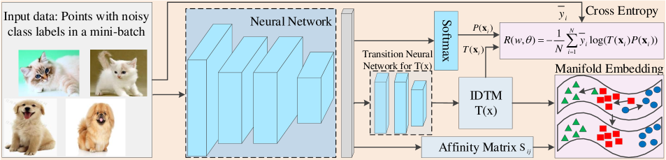
Figure 1: The proposed instance-dependent label-noise learning framework. We train a classifier in a statistically consistent manner through the proposed IDTM $T(\textbf{x})$, where $T(\textbf{x}_{i})\in R^{K\times K}$ is estimated by the transition neural network. It is regularized by the manifold embedding to reduce the degree of freedom of $T(\textbf{x})$ and make it estimable in practice. In the manifold embedding $\mathcal{L}$, the affinity matrix $S_{ij}$ is obtained by finding the $k$-nearest neighbors in the instance feature space. Finally, we use the cross-entropy to train the classifier assisted by $T(\textbf{x})$.

Existing methods have tried to deal with this challenging and ill-posed problem from two perspectives. First, they have simplified the complex problem of estimating a matrix-valued function $T(\textbf{x})$ for the general label noise into a problem of estimating $T$ (i.e., a fixed matrix), which is known as CCN. Then, some anchor points (training data that certainly belong to some specific classes) are adopted to easily estimate the transition matrix $T$ [22, 32]. Although such methods have theoretical guarantees and have achieved success under some synthetic noisy labels or specific conditions, they are unable to cope with general real-world noise, i.e., IDN. Second, several pioneer works considered strong assumptions and focused on how to simplify $T(\textbf{x})$ and significantly reduce its degree of freedom or complexity. For example, in part-dependent noise [44], it is assumed that $T(\textbf{x})$ is a convex combination of a predefined number of fixed transition matrices, and their coefficients come from non-negative matrix factorization. In such a way, the estimation problem becomes parametric, and the degree of freedom of $T(\textbf{x})$ can be reduced. The issue of those methods is that simplifying the form of $T(\textbf{x})$ too much will certainly cause a large approximation error.

To address the problem of estimating IDTM $T(\textbf{x})$ under IDN, in this paper, we will not put any strong assumption on the form of $T(\textbf{x})$, but we will instead put some assumption on the geometry of $T(\textbf{x})$. More specifically, we have noticed that, there are psychological and physiological evidences [24, 6, 30, 36] showing that we humans are more likely to annotate instances of similar appearances to the same class, and thus poor-quality or ambiguous instances of similar appearances are susceptible to be mislabeled to correlated or same noisy classes. Therefore, according to the basic principle that the noisy class-posterior probability $P(\bar{Y}=j|X=\textbf{x})$ can be inferred by the latent clean class-posterior probability $P(Y=i|X=\textbf{x})$ and IDTM $T(\textbf{x})$, we propose an assumption that “the closer two instances are, the more similar their corresponding transition matrices will be”. This can be interpreted as that the instance adjacent relationships of one category in the feature space should be consistent with those in the transition matrix space.

Motivated by this practically useful assumption, we propose to estimate $T(\textbf{x})$ by formulating the assumption into the manifold embedding as shown in Figure 1. Specifically, we make use of the manifold assumption, and require that if $\textbf{x}_{i}$ and $\textbf{x}_{j}$ are close in the feature space, then $T(\textbf{x}_{i})$ and $T(\textbf{x}_{j})$ should also be close (in terms of a matrix norm). Going along this line, though we do not reduce the complexity of $T(\textbf{x})$ directly since we do not further simplify it, we still effectively reduce the degree of freedom of the linear system $P(\bar{y}_{i}|\textbf{x}_{i})=T(\textbf{x}_{i})P(y_{i}|\textbf{x}_{i}),i=1,..,N$ and make $T(\textbf{x})$ stably estimable in practice. Here, $T(\textbf{x})$ can be regarded as practically stable, since adding such a smoothness assumption stops $T(\textbf{x})$ from changing too much in a tiny neighborhood and then it should be Lipschitz continuous. Thus, it should be uniquely determined given infinite data or the underlying data distribution. Finally, we conduct extensive experiments on various datasets, which illustrates the proposed method is superior to state-of-the-art approaches for label-noise learning under IDN.

The main contributions are summarized as follows:

• We are the first to propose the practical assumption on the geometry of $T(\textbf{x})$ that “the closer two instances are, the more similar their corresponding transition matrices should be”, which aims to reduce the degree of freedom of $T(\textbf{x})$, and make it stably estimable in practice.

• We formulate the assumption into manifold embedding, which allows to keep the instance adjacent relationships in the features space to be consistent with those in the transition matrix space. By this way, the proposed manifold-regularized method can greatly reduce the estimation error without hurting much approximation error about the estimation problem of $T(\textbf{x})$.

• Extensive experiments on various datasets demonstrate superior classification performances over current state-of-the-art methods on both synthetic IDN datasets (MNIST, CIFAR10, CIFAR100) and two real-world noisy datasets (Clothing1M and Food101N).

2 Related Works

Typical label-noise models can be categorized as the random classification noise (RCN) model, the CCN model, and the IDN model. In the RCN model, the clean labels flip randomly with a fixed noise rate $\rho\in[0,1/2)$ [15, 1]. The CCN model is a nature extension of the RCN model for multi-class classification [38, 31, 26]. It assumes that the flip rate for each instance from class $i$ to class $j$ depends on the latent clean class. Thus, it is possible to model some similarity information between classes. For example, we expect that the image of a “dog” is more likely to be miss-labeled as "cat" than "boat"[3]. Common methods to handle the CCN model include the “loss correction"  [32, 26] and the “label correction” methods [39, 33]. The IDN model considers more general case of label noise, where the probability of an instance being mislabeled depends on the features and class of the instance itself. Intuitively, IDN is quite realistic and applicable, as the poor-quality and ambiguous instances are more prone to be labeled wrongly in real-world datasets. However, it is very complex to model IDN without any additional assumption. Our work in this paper, aims to estimate this realistic IDN model by considering practical useful assumptions on the geometry of $T(\textbf{x})$, which aims to reduce the degree of freedom of $T(\textbf{x})$, and make it stably estimable in practice.

Estimating the transition matrix is one popular direction to build statistically consistent classifier. It helps to significantly reduce the side-effects of noisy labels, by inferring clean distribution based on the transition matrix and the noisy class-posterior probabilities, statistically. We first review representative works under the CCN. By leveraging the class-dependent transition matrix (CDTM) $T$, the training loss on the noisy data can be corrected. There exist many algorithms to estimate the CDTM $T$ [13, 37, 51, 22, 19, 45]. For example, Liu et al. [22] introduced the anchor points assumption to estimate $T$, Li et al. [19] tried to optimize the transition matrix by minimizing the volume of $T$. To estimate the IDTM $T(\textbf{x})$, existing works rely on various assumptions, for example, Cheng et al. [5] proposed to estimate $T(\textbf{x})$ with a bounded noise rate, Xia et al. [44] proposed to approximate the IDTM $T(\textbf{x})$ by utilizing the part regularization of the transition matrices. Berthon et al. [3] introduced the instance-level forward correction method to estimate $T(\textbf{x})$, Yang et al. [50] proposed to infer the Bayes optimal distribution instead of the clean distribution. Although above advanced methods achieved success empirically, some strong assumptions limit their applications in practice [50]. In contrast, our work proposes a manifold-regularized method to reduce the estimation error without hurting much approximation error of $T(\textbf{x})$, which achieves superior performances for label-noise learning.

Extracting confident clean examples is crucial for optimizing the transition matrix $T(\textbf{x})$ when only noisy data is available. To accurately estimate the transition matrix, we usually require that some clean data of each class are given. When clean data is not available, they are required to be extracted from the noisy data automatically, to construct confident clean dataset for optimizing $T(\textbf{x})$. The current effective methods mainly include but not limited to the following approaches: the distillation method [50], sample sieve approach [5, 25], loss distribution modeling by a Gaussian mixture model [18], confidence-based sample collection [3, 9], small-loss-based methods [41, 11], and some early stopping techniques [2]. When the confident clean examples are obtained, the IDTM $T(\textbf{x})$ for each instance can be learned. Besides, there also exist many other semi-supervised learning methods [18, 28, 5, 8, 10], which transform the label-noise learning into the semi-supervised learning by using the extracted confident clean examples. In this paper, we also need to adopt such a method to extract confident clean examples for optimizing the IDTM $T(\textbf{x})$.

3 Label-Noise Learning Method

In this section, we obtain a statistically consistent classifier through the estimated IDTM $T(\textbf{x})$. Specifically, as illustrated in Figure 1, the proposed method mainly consists of the following components: the input noisy data, confident clean example-extracting module, where we have cast them as a whole in Figure 1, the backbone network and the transition neural network aiming to learn the instance features and estimate $T(\textbf{x})$ respectively, the cross-entropy loss training with noisy labels, and the proposed manifold-regularized objective. Finally, we jointly train the DNN to learn $T(\textbf{x})$ for each instance, and obtain a consistent classifier $f(\textbf{x};\textbf{w})$ on the given noisy data.

3.1 Problem Setting

Define $D$ be the distribution of pair-wise random variables $(\textbf{X},\textbf{Y})\in\mathcal{X}\times\mathcal{Y}$, where X denotes the variable of training samples, Y is the variable of corresponding labels, $\mathcal{X}\in\mathbb{R}^{d}$ and $d$ is the instance feature dimension, $\mathcal{Y}=\{1,2,\ldots,K\}$ and $K$ is the total number of the label classes. The classification problem is to predict the label $y\in\mathcal{Y}$ for each given instance $\textbf{x}\in\mathcal{X}$. However, in some real-world classification problems, it is not easy or even infeasible to directly obtain large-scale training samples independently from the clean distribution $D$, since the clean labels are often randomly corrupted into the noisy labels when being observed.

Define $\bar{D}$ be the distribution of these noisy examples $(\textbf{X},\bar{\textbf{Y}})\in\mathcal{X}\times\bar{\mathcal{Y}}$, where $\bar{\textbf{Y}}$ denotes the random variable of noisy labels. This paper targets at the classification problem when we can only access a set of $N$ training examples with IDN denoted by $\bar{\mathcal{D}}:=\{(\textbf{x}_{i},\bar{y}_{i})\}_{i=1}^{N}$, where examples $(\textbf{x}_{i},\bar{y}_{i})$ is independently drawn according to $\bar{D}$.

The IDTM $T(\textbf{x})$ is defined to build the bridge between the clean distribution $D$ and the noisy distribution $\bar{D}$. As described in Eq. (1), the noisy class-posterior probability $P(\bar{Y}|\textbf{X})$ can be inferred by the IDTM $T(\textbf{x})$ and the clean class-posterior probability $P(Y|\textbf{X})$, where $T(\textbf{x})=(T_{i,j}(\textbf{x}))_{i,j=1}^{K}\in[0,1]^{K\times K}$.

$$P(\bar{Y}=j|\textbf{X}=\textbf{x})=\sum_{i=1}^{K}T_{ij}(\textbf{x})P(Y=i|\textbf{X}=\textbf{x}),$$ (1)

where the IDTM is defined as $T_{ij}(\textbf{x})=P(\bar{Y}=j|Y=i,\textbf{x})$. We can clearly see that $T(\textbf{x})$ depends on the actual instance, and it is tremendously complex as the noise is now characterized by $K^{2}$ functions over the instance feature space $\mathcal{X}$, which can be very high-dimensional.

Therefore, the goal is to obtain a reliable classifier from the noisy training dataset that could classify the test instances accurately, by accurately estimating the IDTM $T(\textbf{x})$. Specifically, in Eq. (1), only the noisy class-posterior probability $P(\bar{Y}|\textbf{X})$ can be obtained by exploiting the noisy data. To accurately estimate $T(\textbf{x})$, there contain two important steps: 1) extracting confident clean examples; 2) optimizing the IDTM $T(\textbf{x})$ based on the given noisy labels and the extracted confident clean examples.

Extracting confident clean examples is very crucial for optimizing the IDTM $T(\textbf{x})$ as can be inferred from Eq. (1). In the related work section, we have listed many useful sample-sieve approaches. In this paper, we adopt the example distillation method [50] to extract confident clean examples. This method can extract a distilled sub-dataset with theoretically guaranteed Bayes optimal labels out of the noisy dataset. Note that our method is not limited to the above distillation-based example extraction method, but many other sample-sieve approaches can also be used. Then, we can train a DNN on the extracted sub-dataset to learn the transition matrix $T(\textbf{x})$ to model the relationships between the confident clean data distribution $D$ and the noisy data distribution $\bar{D}$. Here, we denote as $\bar{\mathcal{D}}^{\mathrm{s}}:=\{(\textbf{x}_{i}^{\mathrm{s}},\bar{y}_{i})\}_{i=1}^{N^{\mathrm{s}}}$ the extracted examples. For simplicity, we still use $\bar{\mathcal{D}}:=\{(\textbf{x}_{i},\bar{y}_{i})\}_{i=1}^{N}$ in the following descriptions.

3.2 The Label-Noise Learning Framework

Given the extracted training examples $\{(\textbf{x}_{i}^{\mathrm{s}},\bar{y}_{i})\}_{i=1}^{N^{\mathrm{s}}}$, we train the transition neural network parameterized by $\theta$ to estimate $T(\textbf{x})$, which models the probability of observing a noisy label $\bar{y}$ from the given input instance x and its corresponding estimated latent clean label $\hat{y}$. Then, it can be expressed as $T_{ij}(\textbf{x};\theta)=P(\bar{Y}=j|\hat{Y}=i,\textbf{X}=\textbf{x};\theta)$, where $T_{ij}(\textbf{x};\theta)\in\mathbb{R}^{K\times K}$, $\hat{Y}$ is the variable for the labels of the extracted confident clean data. To extract confident clean data, we need to learn the noisy class-posterior probability, which can be obtained by a classifier $f(\bullet;\textbf{w})$ parameterised by w, i.e., $P(\hat{Y}|\textbf{x};\textbf{w})=f(\textbf{x};\textbf{w})$.

The probability of observing a noisy label $\bar{Y}$ given the input instance x can be inferred as,

$$P(\bar{Y}=j|\textbf{x})=\sum_{i=1}^{K}P(\bar{Y}=j|\hat{Y}=i,\textbf{x})P(\hat{Y}=i|\textbf{x}).$$ (2)

Obviously, to infer the noisy label $\bar{Y}$ given the instance x, we need to optimize two sets of parameters $\{\textbf{w},\theta\}$, where w is for the classifier $f(\textbf{x};\textbf{w})$, $\theta$ is for the IDTM $T_{ij}(\textbf{x};\theta)=P(\bar{Y}=j|\hat{Y}=i,\textbf{X}=\textbf{x};\theta)$. Traditionally, we could jointly optimize the parameters $(\textbf{w},\theta)$ by minimizing the empirical risk on the inferred noisy labels and the ground-truth noisy labels as follows:

$$\mathop{\min}_{\textbf{w},\theta}R(\textbf{w},\theta)=-\frac{1}{N}\sum_{i=1}^{N}\bar{y}_{i}\log(T(\textbf{x}_{i};\theta)f(\textbf{x}_{i};\textbf{w})),$$ (3)

where $N$ is the number of instances in the extracted confident clean dataset. Intuitively, we can optimize Eq. (3) directly to obtain the parameter set $(\textbf{w},\theta)$. However, the transition matrix $T(\textbf{x};\theta)$ must be hard to learn without any assumption, the ultimate reason is that the degree of freedom of $T(\textbf{x};\theta)$ is too high, and the linear system $P(\bar{y}|\textbf{x}_{i})=T(\textbf{x}_{i})P(\hat{y}_{i}|\textbf{x}_{i}),i=1,...,N$, has the same number of equations and variables. Existing methods focused on how to simplify $T(\textbf{x})$ itself and significantly reduce its degree of freedom or complexity, which will certainly cause an approximation error. While in our work, we will not put any strong restrictions on the form of $T(\textbf{x})$, instead we will put a mild assumption on the geometry of $T(\textbf{x})$ by using the manifold regularization.

3.3 Manifold-Regularized Transition Matrix

Manifold learning typically aims to retain intrinsic neighbouring structures in the underlying lower-dimensional feature space. The classical manifold learning techniques such as LLE [34] and Isomap [40] estimate the local manifolds via justifiable assumptions. Therefore, we adopt the manifold embedding techniques to fulfill our proposed assumption “the closer two instances are, the more similar their corresponding transition matrices will be”, to make the IDTM $T(\textbf{x})$ practically learnable. With the manifold regularization, though we do not reduce the complexity of $T(\textbf{x})$ directly since we do not further model it, we still effectively reduce the degree of freedom of the linear system $P(\bar{y}_{i}|\textbf{x}_{i})=T(\textbf{x}_{i})P(y_{i}|\textbf{x}_{i})$ and make $T(\textbf{x})$ stably estimable. Meanwhile, $T(\textbf{x})$ can be regarded as practically stable, since adding such a smoothness assumption stops $T(\textbf{x})$ from changing too much. It should be uniquely determined given infinite data or the underlying data distribution.

More specifically, we construct an intrinsic affinity graph to characterize the within-manifold consistency and the extrinsic affinity graph to characterize the between manifold relationships [36], respectively. The intrinsic graph is constructed by node adjacency relationships in all the manifolds, where each node is connected to its $k_{1}$-nearest neighbours within the same manifold. The extrinsic graph is constructed using the between-manifold node adjacency relationships from different manifolds. We use the $k_{2}$-nearest neighbors between the $k$-th manifold and the other manifolds.

Specifically, the within-manifold regularization is to fulfil our assumption on the geometry of $T(\textbf{x})$ that “the closer two instances are, the more similar their corresponding transition matrices should be”, and can be expressed as:

$$\mathcal{M}_{I}=\sum_{i,j=1}^{N}S_{ij}^{(I)}||T(\textbf{x}_{i})-T(\textbf{x}_{j})||^{2},$$ (4)

$$S_{ij}^{(I)}=\left\{\begin{array}[]{rcl}1,&{\textrm{if}\>\textbf{x}_{j}\in\mathcal{N}(\textbf{x}_{i},k_{1})\>\textmd{and}\>\bar{y}_{i}=\bar{y}_{j}},\\ 0,&{\textrm{else},}\end{array}\right.$$ (5)

where $S_{ij}^{(I)}$ refers to element $(i,j)$ in the intrinsic affinity graph matrix $\textbf{S}^{I}=(S_{ij}^{(I)})_{N\times N}$, $T(\textbf{x}_{i})$ indicates the IDTM for instance $\textbf{x}_{i}$, $\mathcal{N}(\textbf{x}_{i},k_{1})$ indicates the $k_{1}$-nearest neighbours of the instance $\textbf{x}_{i}$, $\bar{y}_{i}=\bar{y}_{j}$ indicates that $\textbf{x}_{i}$ and $\textbf{x}_{j}$ are in the same manifold, the distance used for computing nearest neighbours is the Euclidean distance between $\textbf{x}_{i}$ and $\textbf{x}_{j}$ in the feature space. Obviously, minimizing the within-manifold consistency encourages the learned IDTM $T(\textbf{x})$ to be close, if their corresponding instances are close in the same category. This keeps the manifold in the instance feature space to be consistent with that in the transition matrix space.

Meanwhile, since instances with different noisy labels correspond to different effective row values in the transition matrix, we also construct a extrinsic graph to characterize the margin between manifolds. It can be expressed as:

$$\mathcal{M}_{B}=\sum_{i,j=1}^{N}S_{ij}^{(B)}||T(\textbf{x}_{i})-T(\textbf{x}_{j})||^{2},$$ (6)

$$S_{ij}^{(B)}=\left\{\begin{array}[]{rcl}1,&{\textrm{if}\>\textbf{x}_{j}\in\mathcal{N}(\textbf{x}_{i},k_{2})\>\textmd{and}\>\bar{y}_{i}\neq\bar{y}_{j}},\\ 0,&{\textrm{else},}\end{array}\right.$$ (7)

where $S_{ij}^{(B)}$ denotes element $(i,j)$ of the between-class affinity matrix $\textbf{S}^{B}=(S_{ij}^{(B)})_{N\times N}$, $\mathcal{N}(\textbf{x}_{i},k_{2})$ indicates the $k_{2}$-nearest neighbours of instance $\textbf{x}_{i}$, $\bar{y}_{i}\neq\bar{y}_{j}$ indicates $\textbf{x}_{i}$ and $\textbf{x}_{j}$ are from different manifolds.

Therefore, the overall proposed manifold-regularization on the IDTM $T(\textbf{x}_{i};\theta)$ can be expressed as:

$$\mathcal{M}(\theta)=\mathcal{M}_{I}-\mathcal{M}_{B}.$$ (8)

We can clearly see that, minimizing the manifold-regularization objective $\mathcal{M}(\theta)$ is equivalent to keep the manifold in the transition matrix space be consistent with that in the feature/label space. Thus, we fulfill the proposed practical useful assumption on the geometry of $T(\textbf{x})$.

Remarks: The manifold embedding is usually used in the unsupervised or semi-supervised learning, its affinity matrix is constructed by the $k$-nearest neighbours in an unsupervised manner traditionally. However, in this work, we construct the affinity matrix for the manifold embedding while considering the given noisy labels as shown in Eq. (5) and Eq. (7). The main reason is that different instances with different given noisy labels correspond to different effective rows in their corresponding transition matrices $T(\textbf{x})$. We only used one row of $T(\textbf{x})$ to generate the noisy label. Then even two instances, $\textbf{x}_{i}$ and $\textbf{x}_{j}$, are very close in the feature space and have the same confident clean label, their corresponding transition matrices should be far apart if they have different given noisy labels. Therefore, we specially design the affinity matrix in the proposed manifold-regularized label-noise learning framework, as shown in Eq.(5), (7), (9) and (10), for optimizing the IDTM $T(\textbf{x})$.

3.4 Kernel Trick to the Manifold Embedding

To improve the effectiveness of the proposed manifold-regularization on the IDTM $T(\textbf{x}_{i};\theta)$ , we further consider to adopt the kernel trick to pre-compute the affinity graph matrix [36]. Concretely, $S_{ij}^{(I)}$ and $S_{ij}^{(B)}$ can be defined as,

$$S_{ij}^{(I)}=\left\{\begin{array}[]{rcl}e^{-\frac{||\textbf{x}_{i}-\textbf{x}_{j}||^{2}}{\sigma^{2}}},&{\textrm{if}\>\textbf{x}_{j}\in\mathcal{N}(\textbf{x}_{i},k_{1})\>\textmd{and}\>\bar{y}_{i}=\bar{y}_{j},}\\ 0,&{\textrm{else},}\end{array}\right.$$ (9)

$$S_{ij}^{(B)}=\left\{\begin{array}[]{rcl}e^{-\frac{||\textbf{x}_{i}-\textbf{x}_{j}||^{2}}{\sigma^{2}}},&\>{\textrm{if}\>\textbf{x}_{j}\in\mathcal{N}(\textbf{x}_{i},k_{2})\>\textmd{and}\>\bar{y}_{i}\neq\bar{y}_{j},}\\ 0,&{\textrm{else},}\end{array}\right.$$ (10)

where $\sigma$ is one hyper-parameter to adjust the weight distribution in the affinity graph matrix.

3.5 Overall Objective Function

Finally, the overall objective function can be expressed as Eq.(11),

$$\mathop{\min}_{\textbf{w},\theta}\mathcal{L}(\textbf{w},\theta)=R(\textbf{w},\theta)+\lambda\mathcal{M}(\theta),$$ (11)

where $\lambda$ is the hyper-parameter to balance the cross-entropy loss and the manifold embedding regularization.

3.6 Optimization

During optimization, the traditional back-propagation method (e.g., SGD) is used to learn the classifier $f(\textbf{x};\textbf{w})$ and the IDTM $T(\textbf{x})$. Therefore, it is required to compute the gradient of the objective function with respect to the output of the corresponding layers.

Define $\textbf{S}=(S_{ij})_{N\times N}=\textbf{S}^{I}-\textbf{S}^{B}$, then the manifold-regularized objective can be re-written as [36],

$$\mathcal{M}=\sum_{i,j=0}^{N}S_{ij}||T(\textbf{x}_{i})-T(\textbf{x}_{j})||^{2}=2tr(\textbf{T}\mathbf{\Phi}\textbf{T}^{T}),$$ (12)

where $\textbf{T}=[T(\textbf{x}_{1}),T(\textbf{x}_{2}),...,T(\textbf{x}_{N})]$, $T(\textbf{x}_{i})\in\mathbb{R}^{K\times K}$ can be reshaped as $K^{2}\times 1$ dimension in T, $\mathbf{\Phi}=\textbf{D}-\textbf{S}$, $\textbf{D}=diag(d_{11},d_{22},...,d_{NN})$, $d_{ii}=\sum_{j=1,i\neq j}^{N}S_{ij},i=1,2,...,N$, $\mathbf{\Phi}$ is the Laplacian matrix of S, and $tr(\cdot)$ denotes the trace of a matrix.

The gradient of $\mathcal{M}(\theta)$ with respect to $T(\textbf{x}_{i})$ can be derived as [36],

$$\frac{\partial\mathcal{M}}{\partial T(\textbf{x}_{i})}=2\textbf{T}(\mathbf{\Phi}+\mathbf{\Phi}^{T})_{(:,i)}=4\textbf{T}\mathbf{\Phi}_{(:,i)},$$ (13)

where $\mathbf{\Phi}_{(:,i)}$ denotes the $i$-th column of matrix $\mathbf{\Phi}$.

Please note that, whether the affinity graph matrix S is in the traditional form or the kernel-wise version, they are pre-computed based on current instance features in the mini-batch. They work as constant values which do not involve in the gradient back-propagation.

  Input: Noisy training dataset $\bar{\mathcal{D}}=\{\textbf{x}_{i},\bar{y}_{i}\}_{i=1}^{N}$

Output: The final classifier $f(\textbf{x};\textbf{w})$ and the transition matrix $T(\textbf{x};\theta)$.

Warmup: Train the DNN on the noisy dataset $\bar{\mathcal{D}}$ with the early-stop strategy to obtain the initial classifier $f(\textbf{x};\textbf{w})$;

while Number of training epoch $\leq$ Max-Epoch do

       $\bullet$ Extract confident clean examples using example distillation method [50] with current classifier $f(\textbf{x};\textbf{w})$ to form the sub-dataset $\bar{\mathcal{D}}^{s}=\{\textbf{x}^{s}_{i},\bar{y}_{i}\}_{i=1}^{N^{s}}$;

      

      $\bullet$ Input the extracted confident clean examples into the backbone network;

      

      $\bullet$ Compute the affinity graph matrix $S_{ij}^{(I)}$ and $S_{ij}^{(B)}$ based on current instance features according to Eq. (5) and (7) or Eq. (9) and (10);

      

      $\bullet$ Optimize the DNN based on the loss function shown in Eq. (11) to obtain new classifier $f(\textbf{x};\textbf{w})$ and transition matrix $T(\textbf{x};\theta)$.

end while

Algorithm 1 Instance-dependent Label-Noise Learning Algorithm

4 Experiments

In this section, we first introduce the experiment setup including the dataset, noisy type and implementation details. Next, we compare the proposed method with the state-of-the-art methods on four synthetic and two real-world noisy datasets, then conduct an ablation study to analyze the experimental results and some useful hyper-parameters.

4.1 Experiment Setup

Datasets. Extensive experiments are conducted to illustrate the effectiveness of our method, on four manually corrupted datasets (i.e., F-MNIST [46],SVHN [27],CIFAR-10 [16], CIFAR-100 [16]) and two real-world noisy datasets ( i.e., Clothing1M [47] and Food-101N [17]). F-MNIST has $28\times 28$ gray scale images of 10 classes including 60K for training and 10K for testing. SVHN contains 10 classes of images with $73,257$ for training and $26,032$ for testing. CIFAR-10 contains 10 classes and CIFAR-100 contain 100 classes, and both of them contain 50K training images and 10K testing images of size 32$\times$ 32. Clothing1M has 1M images with real-world noisy labels from 14 fashion classes for training and 10K test images with clean label, where the estimated noisy label rate is $38.46\%$. Food101N contains 101 food categories with 310k training images and 55K clean images for testing, which is also a real-world noisy dataset and has about $19.66\%$ noisy labels in the training dataset.

Noisy type. For the manually corrupted datasets (i.e., F-MNIST, SVHN, CIFAR-10, and CIFAR-100), we adopt exactly the same strategy to generate the instance-dependent label noise as previous methods [5, 44]. The basic idea is to randomly generate one vector for each class (K vectors for all the classes) and project each instance feature onto the K vectors. The noise label is generated by jointly considering its clean label and the projected results. We have set different noisy rate for all the datasets from $10\%$ to $50\%$ to evaluate all the methods.

Table 1: Comparison with state-of-the-art methods on F-MNIST and CIFAR-10 datasets. The mean and standard deviation computed over five runs are presented. “IDN-xx$\%$” means the noise rate is xx$\%$ and noise type is “IDN”.

Method	F-MNIST					CIFAR-10
	IDN-$10\%$	IDN-$20\%$	IDN-$30\%$	IDN-$40\%$	IDN-$50\%$	IDN-$10\%$	IDN-$20\%$	IDN-$30\%$	IDN-$40\%$	IDN-$50\%$
CE (baseline)	87.73$\pm$ 1.25	87.63$\pm$ 1.11	85.25$\pm$ 0.57	75.00 $\pm$0.25	65.42$\pm$ 1.59	88.86$\pm$ 0.23	86.93$\pm$ 0.17	82.42$\pm$ 0.44	76.68$\pm$ 0.23	58.93$\pm$ 1.54
GCE [54]	90.24 $\pm$0.16	88.71$\pm$ 0.17	85.90$\pm$ 0.23	76.78$\pm$ 0.37	67.67$\pm$ 0.58	90.82$\pm$ 0.05	88.89$\pm$ 0.08	82.90$\pm$ 0.51	74.18$\pm$ 3.10	58.93$\pm$ 2.67
DMI [48]	90.14$\pm$ 0.22	88.13$\pm$ 0.47	85.90$\pm$ 0.23	76.22$\pm$ 0.71	64.84$\pm$ 1.28	91.43$\pm$ 0.18	89.99$\pm$ 0.15	86.87$\pm$ 0.34	80.74$\pm$ 0.44	63.92$\pm$ 3.92
Forward [32]	90.78$\pm$ 0.30	89.01$\pm$ 0.44	86.51$\pm$ 1.20	78.17$\pm$ 0.32	68.31$\pm$ 1.07	91.71$\pm$ 0.08	89.62$\pm$ 0.14	86.93$\pm$ 0.15	80.29$\pm$ 0.27	65.91$\pm$ 1.22
CoTeaching [11]	90.54$\pm$ 0.35	88.53$\pm$ 0.09	87.37$\pm$ 0.14	78.36$\pm$ 0.82	67.81$\pm$ 1.02	90.80$\pm$ 0.05	88.43$\pm$ 0.08	86.40$\pm$ 0.41	80.85$\pm$ 0.97	62.63$\pm$ 1.51
CoTeaching++ [52]	90.67$\pm$0.49	88.52$\pm$ 0.44	87.33$\pm$ 0.87	79.85$\pm$ 1.03	68.86$\pm$ 1.39	91.47$\pm$ 0.59	89.78$\pm$ 0.34	85.72$\pm$ 0.35	81.00$\pm$ 0.82	61.46$\pm$ 1.36
JoCor [43]	91.48$\pm$ 0.11	89.24$\pm$ 0.09	86.50$\pm$ 0.10	77.15$\pm$1.04	67.85$\pm$0.84	91.42$\pm$ 0.11	89.30$\pm$ 0.27	85.54$\pm$ 0.82	80.87$\pm$ 0.91	64.11$\pm$ 2.57
PeerLoss [23]	90.76$\pm$0.41	87.06$\pm$ 0.74	84.40$\pm$ 0.93	73.95$\pm$ 2.37	65.79$\pm$ 2.49	90.89$\pm$ 0.07	89.21$\pm$ 0.63	85.70$\pm$ 0.56	78.51$\pm$ 1.23	59.08$\pm$ 1.05
TMDNN [50]	91.33$\pm$ 0.27	89.70$\pm$ 0.14	87.63$\pm$ 1.28	78.40$\pm$ 3.69	66.55$\pm$ 7.52	90.45$\pm$ 0.72	88.14$\pm$ 0.66	84.55$\pm$0.48	79.71$\pm$ 0.95	63.33$\pm$ 2.75
PartT [44]	91.27$\pm$ 0.38	89.78$\pm$ 0.43	88.30$\pm$ 0.51	80.75$\pm$ 2.86	72.22$\pm$ 4.22	90.32$\pm$ 0.15	89.33$\pm$ 0.70	85.33$\pm$1.86	80.59$\pm$ 0.41	64.58$\pm$ 2.86
MEIDTM (Ours)	91.78$\pm$ 0.87	90.49$\pm$ 0.35	88.74$\pm$ 0.25	84.21$\pm$ 0.52	73.67$\pm$ 3.76	92.17$\pm$ 0.21	91.38$\pm$ 0.34	87.68$\pm$ 0.26	82.63$\pm$ 0.24	72.17$\pm$ 1.51
kMEIDTM (Ours)	91.96$\pm$0.08	90.83$\pm$ 0.05	89.61$\pm$ 0.65	85.81$\pm$ 0.44	76.43$\pm$ 4.88	92.91$\pm$ 0.07	92.26$\pm$ 0.25	90.73$\pm$ 0.34	85.94$\pm$ 0.92	73.77$\pm$ 0.82

Table 2: Comparison with state-of-the-art methods on SVHN and CIFAR-100 datasets. The mean and standard deviation computed over five runs are presented. “IDN-xx$\%$” means the noise rate is xx$\%$ and noise type is “IDN”.

Method	SVHN					CIFAR-100
	IDN-$10\%$	IDN-$20\%$	IDN-$30\%$	IDN-$40\%$	IDN-$50\%$	IDN-$10\%$	IDN-$20\%$	IDN-$30\%$	IDN-$40\%$	IDN-$50\%$
CE (baseline)	90.47$\pm$0.27	89.85$\pm$0.16	86.31$\pm$0.79	80.59$\pm$0.56	64.93$\pm$2.03	66.55$\pm$0.23	63.94$\pm$0.51	61.97$\pm$1.16	58.70$\pm$0.56	56.63$\pm$0.69
GCE [54]	90.82$\pm$0.12	89.48$\pm$0.66	86.92$\pm$0.24	81.95$\pm$1.45	63.20$\pm$2.75	69.18$\pm$0.14	68.35$\pm$0.33	66.35$\pm$0.13	62.09$\pm$0.09	56.68$\pm$0.75
DMI [48]	92.66$\pm$0.58	91.88$\pm$0.42	88.44$\pm$0.85	82.27$\pm$1.54	68.72$\pm$2.32	67.06$\pm$0.46	64.72$\pm$0.64	62.8$\pm$1.46	60.24$\pm$0.63	56.52$\pm$1.18
Forward [32]	92.01$\pm$1.10	90.67$\pm$0.27	86.04$\pm$0.40	83.18$\pm$0.95	70.72$\pm$2.00	67.81$\pm$0.48	67.23$\pm$0.29	65.42$\pm$0.63	62.18$\pm$0.26	58.61$\pm$0.44
CoTeaching [11]	91.11$\pm$0.16	90.88$\pm$0.17	88.21$\pm$0.62	86.46$\pm$1.33	70.04$\pm$1.05	67.91$\pm$0.34	67.40$\pm$0.44	64.13$\pm$0.43	59.98$\pm$0.28	57.48$\pm$0.740
CoTeaching++ [52]	92.64$\pm$0.43	91.59$\pm$0.43	87.55$\pm$1.26	87.69$\pm$1.06	72.36$\pm$1.39	68.67$\pm$0.25	68.30$\pm$0.69	65.77$\pm$0.30	61.75$\pm$0.53	57.94$\pm$0.15
JoCor [43]	93.52$\pm$0.47	93.47$\pm$0.40	89.47$\pm$1.04	88.56$\pm$1.28	73.70$\pm$1.92	68.48$\pm$0.49	67.87$\pm$0.80	65.73$\pm$0.55	61.64$\pm$0.54	57.75$\pm$0.80
PeerLoss [23]	92.59$\pm$0.56	91.67$\pm$0.72	89.86$\pm$0.67	85.44$\pm$0.97	73.91$\pm$2.30	65.64$\pm$1.07	63.83$\pm$0.48	61.64$\pm$0.67	58.30$\pm$0.80	55.41$\pm$0.28
TMDNN [50]	95.51$\pm$0.13	94.83$\pm$0.64	92.43$\pm$0.91	86.91$\pm$1.17	76.53$\pm$2.15	68.42$\pm$0.42	66.62$\pm$0.85	64.72$\pm$0.64	59.38$\pm$0.65	55.68$\pm$1.43
PartT [44]	95.56$\pm$0.45	94.19$\pm$0.20	92.56$\pm$0.83	88.13$\pm$1.56	77.04$\pm$2.56	67.33$\pm$0.33	65.33$\pm$0.59	64.56$\pm$1.55	59.73$\pm$0.76	56.80$\pm$1.32
MEIDTM (Ours)	95.72$\pm$0.40	95.48$\pm$0.01	94.23$\pm$0.27	92.00$\pm$0.10	78.25$\pm$0.35	68.19$\pm$0.32	67.21$\pm$0.38	66.06$\pm$0.77	62.34$\pm$0.18	57.69$\pm$0.51
kMEIDTM (Ours)	96.38$\pm$0.07	95.66$\pm$0.02	94.68$\pm$0.17	92.20$\pm$0.23	80.22$\pm$2.00	69.88$\pm$0.45	69.16$\pm$0.16	66.76$\pm$0.30	63.46$\pm$0.48	59.18$\pm$0.16

4.2 Implementation Details

For fair comparison, we conduct all experiments on NVIDIA GeForce RTX 3090, and all methods are implemented on the same PyTorch platform. The backbone network we used on F-MNIST dataset is ResNet-18, while ResNet-34 network is used on SVHN, CIFAR-10 and CIFAR-100 datasets. For the two real-world dataset (Clothing1M and Food101), we adopt the ResNet-50 network pre-trained on ImageNet as the backbone network. The transition neural network in the framework is implemented by one fully-connected layer, where the input is the instance features, and the number of output nodes is $K\times K$ where $K$ denotes the number of classes on each dataset. The obtained $T(\textbf{x})$ is normalized in each row. The $k$-nearest neighbor parameters in Eq. (5) and Eq. (7) are set as $k_{1}=k_{2}=7$, the hyper-parameter $\sigma$ in Eq. (9) and Eq. (10) is set to 1.1. The optimization strategy we used is SGD with momentum 0.9, weight decay $10^{-3}$, and batch size 128. The initial learning rate is set to $10^{-3}$, which is divided by $10$ every $20$ epochs. Firstly, we train the network on all the noisy data with the early stop techniques as warm-up, where we have trained 5, 10, 20, 1, and 1 epochs on F-MNIST, CIFAR-10, CIFAR-100, Clothing1M and Food101N datasets for warm-up, respectively. Then, we use the initial classifier to extract confident examples from the noisy datasets based on the distillation method [50]. The algorithm flowchart can refer to Alg. 1.

4.3 Comparison with State-of-the-art Methods

We compare our method with the following 10 representative works: 1) CE, which trains the classification network with the standard cross-entropy loss on the original noisy dataset; 2) GCE [54], which uses the mean absolute error and the cross-entropy loss to jointly optimize the model on noisy datasets; 3) DMI [48], which proposed a information-theoretic loss function to robustly train the deep model on the noisy dataset; 4) Forward [32], which utilizes a CDTM $T$ to correct the loss function; 5) Co-teaching [11] and Co-teaching++ [52] propose to train two deep neural networks simultaneously to handle label noise; 6) JoCor [43] adopted a joint training method with co-regularization; 7) PeerLoss [23],which does not require a prior specification of the noise rates; 8) TMDNN [50] and PartT [44] proposed to estimate the IDTM $T(\textbf{x})$ for IDN using DNNs.

Table 3: Classification accuracy ($\%$) on the Clothing1M dataset. (*) indicates that the implementation is based on the authors’ code.

Methods	CE (Baseline)	GCE [54]	SL [42]	Co-teaching [11]	JointOpt [39]	$L_{DMI}$ [48]	PTD-R-V [44]	ERL [21]
Accuracy	68.94	69.75	71.02	69.21	72.16	72.46	71.67	72.87
Methods	ForwardT [32]	JoCor [43]	CORES [5]	CAL [55]	DivideMix* [18]	MEIDTM(Ours)	kMEIDTM(Ours)	kMEIDTM (+DivideMix)
Accuracy	69.84	70.30	73.24	74.17	74.67	73.05	73.34	74.82

Table 4: Classification accuracy ($\%$) on the Food101N dataset.

Methods	Accuracy
CE(Baseline)	81.44
CleanNetWHard(cvpr2018) [17]	83.47
CleanNetWSoft(cvpr2018) [17]	83.95
DeepSelf(cvpr2019) [12]	85.11
NoiseResist(cvpr2021) [20]	84.70
DivideMix(iclr2020)* [18]	84.39
kMEIDTM(+DivideMix) (Ours)	85.61

Results on the synthetic noisy datasets. Table 1,2,4 and 3 report the classification accuracy on datasets of F-MNIST, SVHN, CIFAR-10 and CIFAR-100 under five different noise ratios, respectively. Each table includes 10 representative works on corresponding datasets. Our proposed method has two variants as described in the tables: one is the proposed method with kernel-trick affinity matrix as illustrated in Eq. (9) and (10), which is our final version denoted as “kMEIDTM”; another is the proposed method where the affinity matrix is build by Eq. (5) and Eq. (7), denoted as “MEIDTM”. The baseline method is the standard cross-entropy loss trained on the noisy dataset, denoted as “CE”.

Compared with the representative works, the proposed method achieves top performances on all the four synthesized datasets under five noise ratios. The evaluation results shown in the four tables can be summarized as follows,

• Compared with the best performances shown in previous representative methods, the proposed method kMEIDTM outperforms the former by a margin of 0.48% to 7.67%, and our method outperforms the baseline method “CE” by a large margin of 2.55% to 17.29%.

• The superiority of the proposed method is gradually revealed along with the noise rate increases. As shown in the four table, our method outperforms the second best method by an average margin of 0.64 and 1.04 under IDN-10% and IDN-20%, while 3.12% and 4.69% under IDN-40% and IDN-50%, which illustrate our method can handle extremely hard situation much better.

• Our kernel version kMEIDTM outperforms MEIDTM in almost all situations, by a margin of 0.06% to 2.76%.

Results on the real-world datasets. Table 3 and 4 show the classification results on the real-world Clothing1M and Food101N datasets. It can be seen that the proposed method “MEIDTM” can improve the baseline method “CE” by a margin of $4.11\%$, and then the kernel-wise method “kMEIDTM” further improves the classification accuracy to $73.34\%$.

Since the proposed IDTM estimation method can work as a plug-and-play module, we then integrate this module into the representative work “DivideMix” [18] to further illustrate its effectiveness, denoted as “kMEIDTM(+DivideMix)”. Experimental results show that the proposed transition matrix can further improve the method of “DivideMix” [18] by $0.15\%$ and $1.22\%$ on Clothing1M and Food101N datasets respectively, which is superior to state-of-the-art methods.

4.4 Ablation Study

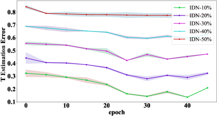
Figure 2: shows the transition matrix estimation error varying with the number of epoches during model training, under five different noise rates, on CIFAR-10 dataset.

To evaluate the estimated IDTM $T(\textbf{x})$, we show the IDTM estimation error during model training under five different noise rates, on CIFAR-10 dataset, in Figure 2. The error is measured by the $l_{1}$ norm between the ground-truth transition matrix and the estimated transition matrix. For each instance, we only analyze the estimation error of a specific low since the noisy is generated by one row of $T(\textbf{x})$. We summary Figure 2 as follows: 1) IDTM estimation error gets smaller and smaller during model training under five noise rates, which illustrate the effectiveness of the proposed method for $T(\textbf{x})$ optimization; 2) the lower noise rate, the better/easier estimation for $T(\textbf{x})$.

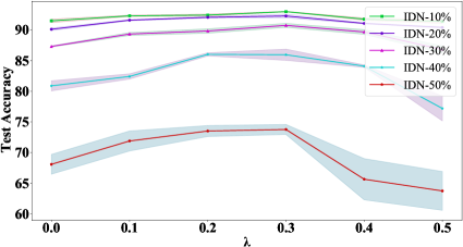
Figure 3: shows the classification accuracy varying with hyper-parameter $\lambda$ under five different noise rates on CIFAR-10 dataset.

To investigate the effect of hyper-parameter $\lambda$ on the model performance, we conduct experiments with various values of $\lambda$ on CIFAR-10 dataset under five noise rates, where each experiment is done with five runs. The results is shown in Figure 3. We can see that the test accuracy is not relatively sensitive to $\lambda$ under low noise rate, i.e., IDN-$10\%$, but it is sensitive under high noise rate, i.e., IDN-$50\%$. Overall, we can clearly see that our method yields the best performance when $\lambda$ is around 0.3. Based on this observation, we set $\lambda=0.3$ in all our experimental evaluations.

5 Conclusion and Limitation

In this paper, we focus on obtaining a consistent classifier under the challenging IDN. To address this problem, we propose the assumption on the geometry of IDTM $T(\textbf{x})$ that “the closer two instances are, the more similar their corresponding transition matrices should be”. Specifically, we formulate the assumption into the manifold embedding to effectively reduce the degree of freedom of $T(\textbf{x})$ and make it stably estimable. This method can directly reduce the estimation error without hurting much approximation error about the estimation problem of $T(\textbf{x})$. Extensive experimental results demonstrate the effectiveness of our method.

Limitation. One major limitation in this study is that we just adopt one fully-connected layer with $K\times K$ output nodes to work as the transition neural network (TNN) for learning $T(\textbf{x})$, which is a little bit simple. In the future, we will make deep analysis on the TNN design theoretically and practically, to learn robust classifier on the noisy dataset.

Acknowledgements: This work was supported in part by the National Key Research and Development Program of China under Grant 2018AAA0103202, in part by the National Natural Science Foundation of China under Grant 62176198, 61922066, 61876142, 62036007 and 62106184, in part by the Technology Innovation Leading Program of Shaanxi under Grant 2022QFY01-15, in part by Open Research Projects of Zhejiang Lab under Grant 2021KG0AB01 and in part by Australian Research Council Projects DE-190101473 and DP-220102121.

References

- [1] Dana Angluin and Philip Laird. Learning from noisy examples. Machine Learning, 2(4):343–370, 1988.
- [2] Yingbin Bai, Erkun Yang, Bo Han, Yanhua Yang, Jiatong Li, Yinian Mao, Gang Niu, and Tongliang Liu. Understanding and improving early stopping for learning with noisy labels. arXiv preprint arXiv:2106.15853, 2021.
- [3] Antonin Berthon, Bo Han, Gang Niu, Tongliang Liu, and Masashi Sugiyama. Confidence scores make instance-dependent label-noise learning possible. In International Conference on Machine Learning, pages 825–836. PMLR, 2021.
- [4] Avrim Blum, Adam Kalai, and Hal Wasserman. Noise-tolerant learning, the parity problem, and the statistical query model. Journal of the ACM (JACM), 50(4):506–519, 2003.
- [5] Hao Cheng, Zhaowei Zhu, Xingyu Li, Yifei Gong, Xing Sun, and Yang Liu. Learning with instance-dependent label noise: A sample sieve approach. ICLR, 2021.
- [6] Uri Cohen, SueYeon Chung, Daniel D Lee, and Haim Sompolinsky. Separability and geometry of object manifolds in deep neural networks. Nature communications, 11(1):1–13, 2020.
- [7] Jacob Goldberger and Ehud Ben-Reuven. Training deep neural-networks using a noise adaptation layer. 2016.
- [8] Sheng Guo, Weilin Huang, Haozhi Zhang, Chenfan Zhuang, Dengke Dong, Matthew R Scott, and Dinglong Huang. Curriculumnet: Weakly supervised learning from large-scale web images. In Proceedings of the European Conference on Computer Vision (ECCV), pages 135–150, 2018.
- [9] Bo Han, Gang Niu, Xingrui Yu, Quanming Yao, Miao Xu, Ivor Tsang, and Masashi Sugiyama. Sigua: Forgetting may make learning with noisy labels more robust. In International Conference on Machine Learning, pages 4006–4016. PMLR, 2020.
- [10] Bo Han, Jiangchao Yao, Gang Niu, Mingyuan Zhou, Ivor Tsang, Ya Zhang, and Masashi Sugiyama. Masking: A new perspective of noisy supervision. arXiv preprint arXiv:1805.08193, 2018.
- [11] Bo Han, Quanming Yao, Xingrui Yu, Gang Niu, Miao Xu, Weihua Hu, Ivor Tsang, and Masashi Sugiyama. Co-teaching: Robust training of deep neural networks with extremely noisy labels. arXiv preprint arXiv:1804.06872, 2018.
- [12] Jiangfan Han, Ping Luo, and Xiaogang Wang. Deep self-learning from noisy labels. In Proceedings of the IEEE/CVF International Conference on Computer Vision, pages 5138–5147, 2019.
- [13] Dan Hendrycks, Mantas Mazeika, Duncan Wilson, and Kevin Gimpel. Using trusted data to train deep networks on labels corrupted by severe noise. arXiv preprint arXiv:1802.05300, 2018.
- [14] Davood Karimi, Haoran Dou, Simon K Warfield, and Ali Gholipour. Deep learning with noisy labels: Exploring techniques and remedies in medical image analysis. Medical Image Analysis, 65:101759, 2020.
- [15] Michael Kearns. Efficient noise-tolerant learning from statistical queries. Journal of the ACM (JACM), 45(6):983–1006, 1998.
- [16] Alex Krizhevsky, Geoffrey Hinton, et al. Learning multiple layers of features from tiny images. 2009.
- [17] Kuang-Huei Lee, Xiaodong He, Lei Zhang, and Linjun Yang. Cleannet: Transfer learning for scalable image classifier training with label noise. In Proceedings of the IEEE Conference on Computer Vision and Pattern Recognition, pages 5447–5456, 2018.
- [18] Junnan Li, Richard Socher, and Steven CH Hoi. Dividemix: Learning with noisy labels as semi-supervised learning. arXiv preprint arXiv:2002.07394, 2020.
- [19] Xuefeng Li, Tongliang Liu, Bo Han, Gang Niu, and Masashi Sugiyama. Provably end-to-end label-noise learning without anchor points. arXiv preprint arXiv:2102.02400, 2021.
- [20] Chang Liu, Han Yu, Boyang Li, Zhiqi Shen, Zhanning Gao, Peiran Ren, Xuansong Xie, Lizhen Cui, and Chunyan Miao. Noise-resistant deep metric learning with ranking-based instance selection. In Proceedings of the IEEE/CVF Conference on Computer Vision and Pattern Recognition, pages 6811–6820, 2021.
- [21] Sheng Liu, Jonathan Niles-Weed, Narges Razavian, and Carlos Fernandez-Granda. Early-learning regularization prevents memorization of noisy labels. arXiv preprint arXiv:2007.00151, 2020.
- [22] Tongliang Liu and Dacheng Tao. Classification with noisy labels by importance reweighting. IEEE Transactions on pattern analysis and machine intelligence, 38(3):447–461, 2015.
- [23] Yang Liu and Hongyi Guo. Peer loss functions: Learning from noisy labels without knowing noise rates. In International Conference on Machine Learning, pages 6226–6236. PMLR, 2020.
- [24] Nikos K Logothetis and David L Sheinberg. Visual object recognition. Annual review of neuroscience, 19(1):577–621, 1996.
- [25] Yueming Lyu and Ivor W Tsang. Curriculum loss: Robust learning and generalization against label corruption. arXiv preprint arXiv:1905.10045, 2019.
- [26] Xingjun Ma, Yisen Wang, Michael E Houle, Shuo Zhou, Sarah Erfani, Shutao Xia, Sudanthi Wijewickrema, and James Bailey. Dimensionality-driven learning with noisy labels. In International Conference on Machine Learning, pages 3355–3364. PMLR, 2018.
- [27] Yuval Netzer, Tao Wang, Adam Coates, Alessandro Bissacco, Bo Wu, and Andrew Y Ng. Reading digits in natural images with unsupervised feature learning. 2011.
- [28] Duc Tam Nguyen, Chaithanya Kumar Mummadi, Thi Phuong Nhung Ngo, Thi Hoai Phuong Nguyen, Laura Beggel, and Thomas Brox. Self: Learning to filter noisy labels with self-ensembling. arXiv preprint arXiv:1910.01842, 2019.
- [29] Curtis G Northcutt, Tailin Wu, and Isaac L Chuang. Learning with confident examples: Rank pruning for robust classification with noisy labels. arXiv preprint arXiv:1705.01936, 2017.
- [30] Stephen E Palmer. Hierarchical structure in perceptual representation. Cognitive psychology, 9(4):441–474, 1977.
- [31] Giorgio Patrini, Frank Nielsen, Richard Nock, and Marcello Carioni. Loss factorization, weakly supervised learning and label noise robustness. In International conference on machine learning, pages 708–717. PMLR, 2016.
- [32] Giorgio Patrini, Alessandro Rozza, Aditya Krishna Menon, Richard Nock, and Lizhen Qu. Making deep neural networks robust to label noise: A loss correction approach. In Proceedings of the IEEE conference on computer vision and pattern recognition, pages 1944–1952, 2017.
- [33] Scott Reed, Honglak Lee, Dragomir Anguelov, Christian Szegedy, Dumitru Erhan, and Andrew Rabinovich. Training deep neural networks on noisy labels with bootstrapping. arXiv preprint arXiv:1412.6596, 2014.
- [34] Sam T Roweis and Lawrence K Saul. Nonlinear dimensionality reduction by locally linear embedding. science, 290(5500):2323–2326, 2000.
- [35] Clayton Scott, Gilles Blanchard, and Gregory Handy. Classification with asymmetric label noise: Consistency and maximal denoising. In Conference on learning theory, pages 489–511. PMLR, 2013.
- [36] Weiwei Shi, Yihong Gong, and Jinjun Wang. Improving cnn performance with min-max objective. In IJCAI, pages 2004–2010, 2016.
- [37] Jun Shu, Qian Zhao, Zongben Xu, and Deyu Meng. Meta transition adaptation for robust deep learning with noisy labels. arXiv preprint arXiv:2006.05697, 2020.
- [38] Guillaume Stempfel and Liva Ralaivola. Learning svms from sloppily labeled data. In International conference on artificial neural networks, pages 884–893. Springer, 2009.
- [39] Daiki Tanaka, Daiki Ikami, Toshihiko Yamasaki, and Kiyoharu Aizawa. Joint optimization framework for learning with noisy labels. In Proceedings of the IEEE Conference on Computer Vision and Pattern Recognition, pages 5552–5560, 2018.
- [40] Joshua B Tenenbaum, Vin De Silva, and John C Langford. A global geometric framework for nonlinear dimensionality reduction. science, 290(5500):2319–2323, 2000.
- [41] Xiaobo Wang, Shuo Wang, Jun Wang, Hailin Shi, and Tao Mei. Co-mining: Deep face recognition with noisy labels. In Proceedings of the IEEE/CVF International Conference on Computer Vision, pages 9358–9367, 2019.
- [42] Yisen Wang, Xingjun Ma, Zaiyi Chen, Yuan Luo, Jinfeng Yi, and James Bailey. Symmetric cross entropy for robust learning with noisy labels. In Proceedings of the IEEE/CVF International Conference on Computer Vision, pages 322–330, 2019.
- [43] Hongxin Wei, Lei Feng, Xiangyu Chen, and Bo An. Combating noisy labels by agreement: A joint training method with co-regularization. In Proceedings of the IEEE/CVF Conference on Computer Vision and Pattern Recognition, pages 13726–13735, 2020.
- [44] Xiaobo Xia, Tongliang Liu, Bo Han, Nannan Wang, Mingming Gong, Haifeng Liu, Gang Niu, Dacheng Tao, and Masashi Sugiyama. Part-dependent label noise: Towards instance-dependent label noise. Advances in Neural Information Processing Systems, 33, 2020.
- [45] Xiaobo Xia, Tongliang Liu, Nannan Wang, Bo Han, Chen Gong, Gang Niu, and Masashi Sugiyama. Are anchor points really indispensable in label-noise learning? Advances in Neural Information Processing Systems, 32:6838–6849, 2019.
- [46] Han Xiao, Kashif Rasul, and Roland Vollgraf. Fashion-mnist: a novel image dataset for benchmarking machine learning algorithms. arXiv preprint arXiv:1708.07747, 2017.
- [47] Tong Xiao, Tian Xia, Yi Yang, Chang Huang, and Xiaogang Wang. Learning from massive noisy labeled data for image classification. In Proceedings of the IEEE conference on computer vision and pattern recognition, pages 2691–2699, 2015.
- [48] Yilun Xu, Peng Cao, Yuqing Kong, and Yizhou Wang. L_dmi: A novel information-theoretic loss function for training deep nets robust to label noise. In NeurIPS, pages 6222–6233, 2019.
- [49] Yan Yan, Rómer Rosales, Glenn Fung, Ramanathan Subramanian, and Jennifer Dy. Learning from multiple annotators with varying expertise. Machine learning, 95(3):291–327, 2014.
- [50] Shuo Yang, Erkun Yang, Bo Han, Yang Liu, Min Xu, Gang Niu, and Tongliang Liu. Estimating instance-dependent label-noise transition matrix using dnns. arXiv preprint arXiv:2105.13001, 2021.
- [51] Yu Yao, Tongliang Liu, Bo Han, Mingming Gong, Jiankang Deng, Gang Niu, and Masashi Sugiyama. Dual t: Reducing estimation error for transition matrix in label-noise learning. arXiv preprint arXiv:2006.07805, 2020.
- [52] Xingrui Yu, Bo Han, Jiangchao Yao, Gang Niu, Ivor Tsang, and Masashi Sugiyama. How does disagreement help generalization against label corruption? In International Conference on Machine Learning, pages 7164–7173. PMLR, 2019.
- [53] Xiyu Yu, Tongliang Liu, Mingming Gong, and Dacheng Tao. Learning with biased complementary labels. In Proceedings of the European conference on computer vision (ECCV), pages 68–83, 2018.
- [54] Zhilu Zhang and Mert R Sabuncu. Generalized cross entropy loss for training deep neural networks with noisy labels. In 32nd Conference on Neural Information Processing Systems (NeurIPS), 2018.
- [55] Zhaowei Zhu, Tongliang Liu, and Yang Liu. A second-order approach to learning with instance-dependent label noise. In Proceedings of the IEEE/CVF Conference on Computer Vision and Pattern Recognition, pages 10113–10123, 2021.