Blended Latent Diffusion

Abstract.

The tremendous progress in neural image generation, coupled with the emergence of seemingly omnipotent vision-language models has finally enabled text-based interfaces for creating and editing images. Handling generic images requires a diverse underlying generative model, hence the latest works utilize diffusion models, which were shown to surpass GANs in terms of diversity. One major drawback of diffusion models, however, is their relatively slow inference time. In this paper, we present an accelerated solution to the task of local text-driven editing of generic images, where the desired edits are confined to a user-provided mask. Our solution leverages a text-to-image Latent Diffusion Model (LDM), which speeds up diffusion by operating in a lower-dimensional latent space and eliminating the need for resource-intensive CLIP gradient calculations at each diffusion step. We first enable LDM to perform local image edits by blending the latents at each step, similarly to Blended Diffusion. Next we propose an optimization-based solution for the inherent inability of LDM to accurately reconstruct images. Finally, we address the scenario of performing local edits using thin masks. We evaluate our method against the available baselines both qualitatively and quantitatively and demonstrate that in addition to being faster, it produces more precise results.

&

Input image	Input mask	“a man with	“a man with	“a muscular man
		a red suit”	a yellow sweater”	with a blue shirt”

Input image	Input mask	a horror book	a children’s book	a romantic novel
		named CVPR	titled ECCV	titled SIGGRAPH

Input image	Input mask	“beach”	“big mountain”	“The Great
				Pyramid of Giza”

Input image	Input mask	Prediction 1	Prediction 2	Prediction 3

Original image	Scribbled image	Mask	Prediction 1	Prediction 2

Figure 1. Applications of our method: (top left) adding a new object in a masked area, guided by a text prompt; (top right) altering a part within an existing object; (middle left) generation of text; (middle right) altering the background in the scene; (bottom left) generating multiple predictions for the same text prompt (“stones”); (bottom right) guiding the result by a combination of text (“paint splashes”) and scribbles.

1. Introduction

In recent years we have witnessed tremendous progress in realistic image synthesis and image manipulation with deep neural generative models. GAN-based models were first to emerge (Goodfellow et al., 2014; Brock et al., 2018; Karras et al., 2019, 2020), soon followed by diffusion-based models (Sohl-Dickstein et al., 2015; Ho et al., 2020; Nichol and Dhariwal, 2021). In parallel, recent vision-language models, such as CLIP (Radford et al., 2021), have paved the way for generating and editing images using a fundamental form of human communication — natural language. The resulting text-guided image generation and manipulation approaches, e.g., (Patashnik et al., 2021; Nichol et al., 2021; Ramesh et al., 2022; Saharia et al., 2022b; Yu et al., 2022; Ding et al., 2021), enable artists to simply convey their intent in natural language, potentially saving hours of painstaking manual work. Figure 1 shows a few examples.

However, the vast majority of text-guided approaches focus on generating images from scratch or on manipulating existing images globally. The local editing scenario, where the artist is only interested in modifying a part of a generic image, while preserving the remaining parts, has not received nearly as much attention, despite the ubiquity of this use case in practice. We know of only three methods to date that explicitly address the local editing scenario: Blended Diffusion (Avrahami et al., 2022b), GLIDE (Nichol et al., 2021) and DALL$\cdot$E 2 (Ramesh et al., 2022). Among these, only Blended Diffusion is publicly available in full.

All three local editing approaches above are based on diffusion models (Sohl-Dickstein et al., 2015; Nichol and Dhariwal, 2021; Ho et al., 2020). While diffusion models have shown impressive results on generation, editing, and other tasks (Section 2), they suffer from long inference times, due to the iterative diffusion process that is applied at the pixel level to generate each result. Some recent works (Rombach et al., 2022; Gu et al., 2021; Esser et al., 2021b; Bond-Taylor et al., 2021; Hu et al., 2021; Vahdat et al., 2021) have thus proposed to perform the diffusion in a latent space with lower dimensions and higher-level semantics, compared to pixels, yielding competitive performance on various tasks with much lower training and inference times. In particular, Latent Diffusion Models (LDM) (Rombach et al., 2022) offer this appealing combination of competitive image quality with fast inference, however, this approach targets text-to-image generation from scratch, rather than global image manipulation, let alone local editing.

In this work, we harness the merits of LDM to the task of local text-guided natural image editing, where the user provides the image to be edited, a natural language text prompt, and a mask indicating an area to which the edit should be confined. Our approach is “zero-shot”, since it relies on available pretrained models, and requires no further training. We first show how to adapt the Blended Diffusion approach of Avrahami et al. (2022b) to work in the latent space of LDM, instead of working at the pixel level.

Next, we address the imperfect reconstruction inherent to LDM, due to the use of VAE-based lossy latent encodings. This is especially problematic when the original image contains areas to which human perception is particularly sensitive (e.g., faces or text) or other non-random high frequency details. We present an approach that employs latent optimization to effectively mitigate this issue.

Then, we address the challenge of performing local edits inside thin masks. Such masks are essential when the desired edit is highly localized, but they present a difficulty when working in a latent space with lower spatial resolution. To overcome this issue, we propose a solution that starts with a dilated mask, and gradually shrinks it as the diffusion process progresses.

Finally, we evaluate our method against the baselines both qualitatively and quantitatively, using new metrics for text-driven editing methods that we propose: precision and diversity. We demonstrate that our method is not only faster than the baselines, but also achieves better precision.

In summary, the main contribution of this paper are: (1) Adapting the text-to-image LDM to the task of local text-guided image editing. (2) Addressing the inherent problem of inaccurate reconstruction in LDM, which severely limits the applicability of this method. (3) Addressing the case when the method is fed by a thin mask, based on our investigation of the diffusion dynamics. (4) Proposing new evaluation metrics for quantitative comparisons between local text-driven editing methods.

2. Related Work

Text-to-image synthesis and global editing: Text-to-image synthesis has advanced tremendously in recent years. Seminal works based on RNNs (Mansimov et al., 2016) and GANs (Reed et al., 2016; Zhang et al., 2017, 2018b; Xu et al., 2018), were later superseded by transformer-based approaches (Vaswani et al., 2017). DALL$\cdot$E (Ramesh et al., 2021) proposed a two-stage approach: first, train a discrete VAE (van den Oord et al., 2017; Razavi et al., 2019) to learn a rich semantic context, then train a transformer model to autoregressively model the joint distribution over the text and image tokens.

Another line of works is based on CLIP (Radford et al., 2021), a vision-language model that learns a rich shared embedding space for images and text, by contrastive training on a dataset of 400 million (image, text) pairs collected from the internet. Some of them (Patashnik et al., 2021; Crowson et al., 2022; Crowson, 2021; Liu et al., 2021; Murdock, 2021; Paiss et al., 2022) combine a pretrained generative model (Brock et al., 2018; Esser et al., 2021a; Dhariwal and Nichol, 2021) with a CLIP model to steer the generative model to perform text-to-image synthesis. Utilizing CLIP along with a generative model was also used for text-based domain adaptation (Gal et al., 2022) and text-to-image without training on text data (Zhou et al., 2021; Wang et al., 2022; Ashual et al., 2022). Make-a-scene (Gafni et al., 2022) first predicts the segmentation mask, conditioned on the text, and then uses the generated mask along with the text to generate the predicted image. SpaText (Avrahami et al., 2022a) extends Make-a-scene to support free-form text prompt per segment. These works do not address our setting of local text-guided image editing.

Diffusion models were also used for various global image-editing applications: ILVR (Choi et al., 2021) demonstrates how to condition a DDPM model on an input image for image translation tasks. Palette (Saharia et al., 2022a) trains a designated diffusion model to perform four image-to-image translation tasks, namely colorization, inpainting, uncropping, and JPEG restoration. SDEdit (Meng et al., 2021) demonstrates stroke painting to image, image compositing, and stroke-based editing. RePaint (Lugmayr et al., 2022) uses a diffusion model for free-form inpainting of images. None of the above methods tackle the problem of local text-driven image editing.

Local text-guided image manipulation: Paint By Word (Bau et al., 2021) was first to address the problem of zero-shot local text-guided image manipulation by combining BigGAN / StyleGAN with CLIP and editing only the part of the feature map that corresponds to the input mask. However, this method only operated on generated images as input, and used a separate generative model per input domain. Later, Blended Diffusion (Avrahami et al., 2022b) was proposed as the first solution for local text-guided editing of real generic images; this approach is further described in Section 3.

Text2LIVE (Bar-Tal et al., 2022) enables editing the appearance of an object within an image, without relying on a pretrained generative model. They mainly focus on changing the colors/textures of an existing object or adding effects such as fire/smoke, and not on editing a general scene by removing objects or replacing them with new ones, as we do.

More related to our work are the recent GLIDE (Nichol et al., 2021) and DALL$\cdot$E 2 (Ramesh et al., 2022) works. GLIDE employs a two-stage diffusion-based approach for text-to-image synthesis: the first stage generates a low-resolution version of the image, while the second stage generates a higher resolution version of the image, conditioned on both the low-resolution version and the guiding text. In addition, they fine-tune their model specifically for the task of local editing by a guiding text prompt. Currently, only GLIDE-filtered, a smaller version of their model (300M parameters instead of 5B), which was trained on a smaller filtered dataset, has been released. As we demonstrate in Section 5, GLIDE-filtered often fails to obtain the desired edits. DALL$\cdot$E 2 performs text-to-image synthesis by mapping text prompts into CLIP image embeddings, followed by decoding such embeddings to images. The DALL$\cdot$E 2 website (OpenAI, 2022a) shows some examples of local text-guided image editing; however, this is not discussed in the paper (Ramesh et al., 2022). Furthermore, neither of their two models has been released. The only available resource is their online demo (OpenAI, 2022a) that is free for a small number of images, which we use for comparisons (Figure 8).

The concurrent prompt-to-prompt work (Hertz et al., 2022) enables editing of generated images without input masks, given a source text prompt and a target text prompt. In contrast, our method enables editing real images, given only a target prompt and a mask.

In summary, at the time of this writing, the only publicly available models that address our setting are Blended Diffusion and GLIDE-filtered.

(a) Input image	(b) Input mask	(c) Blended Diffusion	(d) Ours

Figure 2. Noise artifacts: Given the input image (a) and mask (b) with the guiding text “curly blond hair”, Blended Diffusion produces noticeable pixel-level noise artifacts (c), in contrast to our method (d).

3. Latent Diffusion and Blended Diffusion

Diffusion models are deep generative models that sample from the desired distribution by learning to reverse a gradual noising process. Starting from a standard normal distribution noise $x_{T}$, a series of less-noisy latents, $x_{T-1},...,x_{0}$, are produced. For more details, please refer to (Ho et al., 2020; Nichol and Dhariwal, 2021).

Traditional diffusion models operate directly in the pixel space, hence their optimization often consumes hundreds of GPU days and their inference times are long. To enable faster training and inference on limited computational resources, Rombach et al. (2022) proposed Latent Diffusion Models (LDMs). They first perform perceptual image compression, using an autoencoder (VAE (Kingma and Welling, 2013) or VQ-VAE (Razavi et al., 2019; Van Den Oord et al., 2017; Esser et al., 2021a)). Next, a diffusion model is used that operates on the lower-dimensional latent space. They also demonstrate the ability to train a conditional diffusion model on various modalities (e.g., semantic maps, images, or texts), s.t. when they combine it with the autoencoder they create image-to-image / semantic-map-to-image / text-to-image transitions.

Blended Diffusion (Avrahami et al., 2022b) addresses zero-shot text-guided local image editing. This approach utilizes a diffusion model trained on ImageNet (Deng et al., 2009), which serves as a prior for the manifold of the natural images, and a CLIP model (Radford et al., 2021), which navigates the diffusion model towards the desired text-specified outcome. In order to create a seamless result where only the masked region is modified to comply with the guiding text prompt, each of the noisy images progressively generated by the CLIP-guided process is spatially blended with the corresponding noisy version of the input image. The main limitations of this method is its slow inference time (about 25 minutes using a GPU) and its pixel-level noise artifacts (see Figure 2).

In the next section, we leverage the trained LDM text-to-image model of Rombach et al. (2022) to offer a solution for zero-shot text-guided local image editing by incorporating the idea of blending the diffusion latents from Avrahami et al. (2022b) into the LDM latent space (Section 4.1) and mitigating the artifacts inherent to working in that space (Sections 4.2 and 4.3).

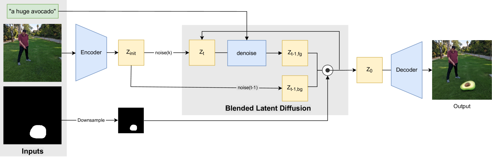
Figure 3. Blended Latent Diffusion: a diagram illustrating our method, as described in Algorithm 1.

  Input: source image $x$, target text description $d$, input mask $m$, diffusion steps $k$.

  Output: edited image $\widehat{x}$ that differs from input image $x$ inside area $m$ according to text description $d$

  

  $m_{\textit{latent}}=\textit{downsample}(m)$

  $z_{\textit{init}}\sim E(x)$

  $z_{k}\sim\textit{noise}(z_{\textit{init}},k)$

  for all $t$ from $k$ to 0 do

     $z_{\textit{fg}}\sim\textit{denoise}(z_{t},d,t)$

     $z_{\textit{bg}}\sim\textit{noise}(z_{\textit{init}},t)$

     $z_{t}\leftarrow z_{\textit{fg}}\odot m_{\textit{latent}}+z_{\textit{bg}}\odot(1-m_{\textit{latent}})$

  end for

  $\widehat{x}=D(z_{0})$

  return  $\widehat{x}$

  

ALGORITHM 1 Latent Blended Diffusion: given a text-conditioned Latent Diffusion model $\{\textit{VAE}=(E(x),D(z)),\textit{DiffusionModel}=(\textit{noise}(z,t),\textit{denoise}(z,d,t))\}$

Input image	Input mask	(a) VAE reconstruction	(b) Edit result	(c) Pixel blending	(d) Poisson blending	(e) Latent optimization	(f) Weights optimization

Figure 4. Background reconstruction comparison: Given the input image, mask, and guiding text prompt “red hair”, the reconstruction does not preserve the unmasked area details (a,b). Pixel-level blending yields a result (c) with noticeable seams. Poisson seamless cloning (d) changes the colors of the edited area, while latent optimization (e) produces an over smoothed result. We propose per-sample weights optimization (f) which produces the best results.

4. Method

Given an image $x$, a guiding text prompt $d$ and a binary mask $m$ that marks the region of interest in the image, our goal is to produce a modified image $\hat{x}$, s.t. the content $\hat{x}\odot m$ is consistent with the text description $d$, while the complementary area remains close to the source image, i.e., $x\odot(1-m)\approx\hat{x}\odot(1-m)$, where $\odot$ is element-wise multiplication. Furthermore, the transition between the two areas of $\hat{x}$ should ideally appear seamless.

In Section 4.1 we start by incorporating Blended Diffusion (Avrahami et al., 2022b) into Latent Diffusion (Rombach et al., 2022) in order to achieve local text-driven editing. The resulting method fails to achieve satisfying results in some cases; specifically, the reconstruction of the complementary area is imperfect, and the method struggles when the input mask $m$ contains thin parts. We solve these issues in Sections 4.2 and 4.3, respectively.

4.1. Blended Latent Diffusion

As explained in Section 3, Latent Diffusion (Rombach et al., 2022) can generate an image from a given text (text-to-image LDM). However, this model lacks the capability of editing an existing image in a local fashion, hence we propose to incorporate Blended Diffusion (Avrahami et al., 2022b) into text-to-image LDM. Our approach is summarized in Algorithm 1, and depicted as a diagram in Figure 3.

LDM performs text-guided denoising diffusion in the latent space learned by a variational auto-encoder $\textit{VAE}=(E(x),D(z))$, where $E(x)$ encodes an image $x$ to a latent representation $z$ and $D(z)$ decodes it back to the pixel space. Referring to the part that we wish to modify as foreground (fg) and to the remaining part as background (bg), we follow the idea of Blended Diffusion and repeatedly blend the two parts in this latent space, as the diffusion progresses. The input image $x$ is encoded into the latent space using the VAE encoder $z_{\textit{init}}\sim E(x)$. The latent space still has spatial dimensions (due to the convolutional nature of the VAE), however the width and the height are smaller than those of the input image (by a factor of 8). We therefore downsample the input mask $m$ to these spatial dimensions to obtain the latent space binary mask $m_{\textit{latent}}$, which will be used to perform the blending.

Now, we noise the initial latent $z_{\textit{init}}$ to the desired noise level (in a single step) and manipulate the denoising diffusion process in the following way: at each step, we first perform a latent denoising step, conditioned directly on the guiding text prompt $d$, to obtain a less noisy foreground latent denoted as $z_{\textit{fg}}$, while also noising the original latent $z_{\textit{init}}$ to the current noise level to obtain a noisy background latent $z_{\textit{bg}}$. The two latents are then blended using the resized mask, i.e. $z_{\textit{fg}}\odot m_{\textit{latent}}+z_{\textit{bg}}\odot(1-m_{\textit{latent}})$, to yield the latent for the next latent diffusion step. Similarly to Blended Diffusion, at each denoising step the entire latent is modified, but the subsequent blending enforces the parts outside $m_{\textit{latent}}$ to remain the same. While the resulting blended latent is not guaranteed to be coherent, the next latent denoising step makes it so. Once the latent diffusion process terminates, we decode the resultant latent to the output image using the decoder $D(z)$. A visualization of the diffusion process is available in the supplementary material.

Operating on the latent level, in comparison to operating directly on pixels using a CLIP model, has the following main advantages:

Faster inference: The smaller dimension of the latent space makes the diffusion process much faster. In addition, there is no need to calculate the CLIP-loss gradients at each denoising step. Thus, the entire editing process is faster by an order of magnitude (see Section 5.2).

Avoiding pixel-level artifacts: Pixel-level diffusion sometimes results in pixel values outside the valid range, producing noticeable clipping artifacts. Operating in the latent space avoids such artifacts (Figure 2).

Avoiding adversarial examples: Operating on the latent space with no pixel-level CLIP-loss gradients effectively eliminates the risk of adversarial examples, eliminating the need for the extending augmentations of Avrahami et al. (2022b).

Better precision: Our method achieves better precision than the baselines, both at the batch level and at the final prediction level (Section 5).

However, operating in latent space also introduces some drawbacks, which we will address later in this section:

Imperfect reconstruction: The VAE latent encoding is lossy; hence, the final results are upper-bounded by the decoder’s reconstruction abilities. Even the initial reconstruction, before performing any diffusion, often visibly differs from the input. In images of human faces, or images with high frequencies, even such slight changes may be perceptible (see Figure 4(b)).

Thin masks: When the input mask $m$ is relatively thin (and its downscaled version $m_{\textit{latent}}$ can become even thinner), the effect of the edit might be limited or non-existent (see Figure 7).

AAatext “GAN”
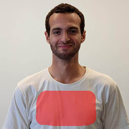
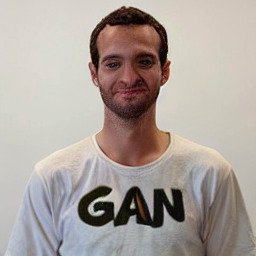
AA “sculpture”
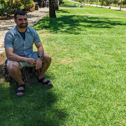
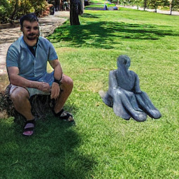
AAA“cucumber”
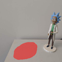
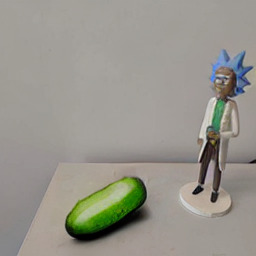
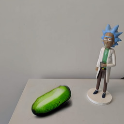
a“heart wall painting”
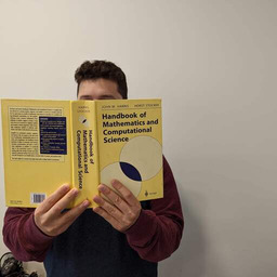
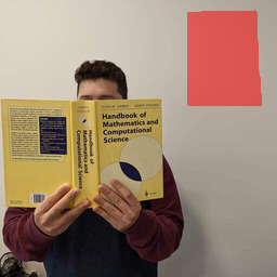
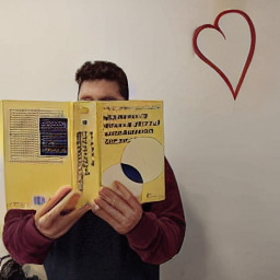
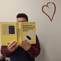
Aa“corgi painting”
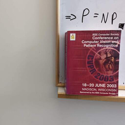
	Input image	Input mask	Initial prediction	After reconstruction

Figure 5. Background reconstruction using decoder weights fine-tuning: Note the bad initial prediction of the high-frequency background areas: the human face in the 1st and 2nd rows, the doll face in the 3rd row, and the text on the books on the 4th and 5th (zoom in for a better presentation).

4.2. Background Reconstruction

As discussed above, LDM’s latent representation is obtained using a VAE (Kingma and Welling, 2013), which is lossy. As a result, the encoded image is not reconstructed exactly, even before any latent diffusion takes place (Figure 4(a)). The imperfect reconstruction may thus be visible in areas outside the mask (Figure 4(b)).

A naïve way to deal with this problem is to stitch the original image and the edited result $\hat{x}$ at the pixel level, using the input mask $m$. However, because the unmasked areas were not generated by the decoder, there is no guarantee that the generated part will blend seamlessly with the surrounding background. Indeed, this naïve stitching produces visible seams, as demonstrated in Figure 4(c).

Alternatively, one could perform seamless cloning between the edited region and the original, e.g., utilizing Poisson Image Editing (Pérez et al., 2003), which uses gradient-domain reconstruction in pixel space. However, this often results in a noticeable color shift of the edited area, as demonstrated in Figure 4(d).

In the GAN inversion literature (Abdal et al., 2019, 2020; Zhu et al., 2020; Xia et al., 2021) it is standard practice to achieve image reconstruction via latent-space optimization. In theory, latent optimization can also be used to perform seamless cloning, as a post-process step: given the input image $x$, the mask $m$, and the edited image $\hat{x}$, along with its corresponding latent vector $z_{0}$, one could use latent optimization to search for a better vector $z^{*}$, s.t. the masked area will be similar to the edited image $\hat{x}$ and the unmasked area will be similar to the input image $x$:

(1) $$z^{*}=\operatornamewithlimits{argmin}\limits_{z}\|D(z)\odot m-\hat{x}\odot m\|\;$$

λ∥D(z)⊙(1-m)-x⊙(1-m)∥

using a standard distance metric, such as MSE. $\lambda$ is a hyperparameter that controls the importance of the background preservation, which we set to $\lambda=100$ for all our results and comparisons. The optimization process is initialized with $z^{*}=z_{0}$. The final image is then inferred from $z^{*}$ using the decoder: $x^{*}=D(z^{*}).$ However, as we can see in Figure 4(e), even though the resulting image is closer to the input image, it is over-smoothed.

The inability of latent space optimization to capture the high-frequency details suggests that the expressivity of the decoder $D(z)$ is limited. This leads us again to draw inspiration from GAN inversion literature — it was shown (Bau et al., 2020; Pan et al., 2021; Roich et al., 2021; Tzaban et al., 2022) that fine-tuning the GAN generator weights per image results in a better reconstruction. Inspired by this approach, we can achieve seamless cloning by fine-tuning the decoder’s weights $\theta$ on a per-image basis:

(2) $$\theta^{*}=\operatornamewithlimits{argmin}\limits_{\theta}\|D_{\theta}(z_{0})\odot m-\hat{x}\odot m\|\;$$

λ∥Dθ(z0)⊙(1-m)-x⊙(1-m)∥

and use these weights to infer the result $x^{*}=D_{\theta^{*}}(z_{0})$. As we can see in Figure 4(f), this method yields the best result: the foreground region follows $\hat{x}$, while the background preserves the fine details from the input image $x$, and the blending appears seamless.

In contrast to Blended Diffusion (Avrahami et al., 2022b), in our method the background reconstruction is optional. Thus, it is only needed in cases where the unmasked area contains perceptually important fine-detail content, such as faces, text, structured textures, etc. A few reconstruction examples are shown in Figure 5.

4.3. Progressive Mask Shrinking

	early steps				final steps
A(1) Standard
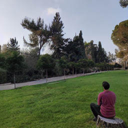
(2) Pro. shrinking
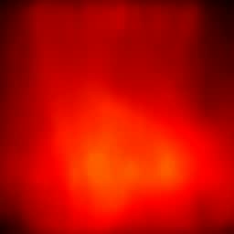
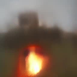
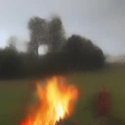
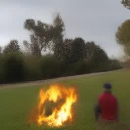
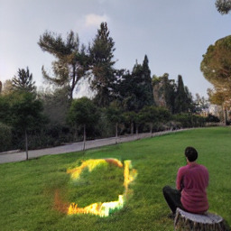
Aa(3) Masks
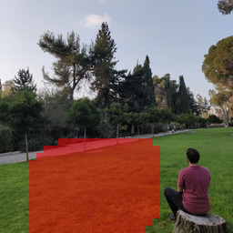
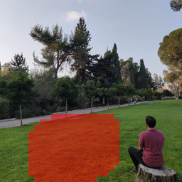
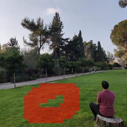
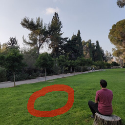
	dilated mask				original mask

Figure 6. Thin mask progression: Given the input image, mask (bottom right corner), and guiding text “fire”, in the standard case (1) only the initial stages correspond to the text (rough red colors), but later the blending overrides it. In contrast, using our progressively shrinking masks (3) the guiding text corresponds to all the images throughout the diffusion process (2).

When the input mask $m$ has thin parts, these parts may become even thinner in its downscaled version $m_{\textit{latent}}$, to the point that changing the latent values under $m_{\textit{latent}}$ by the text-driven diffusion process fails to produce a visible change in the reconstructed result. In order to pinpoint the root-cause, we visualize the diffusion process: given a noisy latent $z_{t}$ at timestep $t$, we can estimate $z_{0}$ using a single diffusion step with the closed form formula derived by Song et al. (2020). The corresponding image is then inferred using the VAE decoder $D(z_{0})$.

Using the above visualization, Figure 6 shows that during the denoising process, the earlier steps generate only rough colors and shapes, which are gradually refined to the final output. The top row shows that even though the guiding text “fire” is echoed in the latents early in the process, blending these latents with $z_{\textit{bg}}$ using a thin $m_{\textit{latent}}$ mask may cause the effect to disappear.

This understanding suggests the idea of progressive mask shrinking: because the early noisy latents correspond to only the rough colors and shapes, we start with a rough, dilated version of $m_{\textit{latent}}$, and gradually shrink it as the diffusion process progresses, s.t. only the last denoising steps employ the thin $m_{\textit{latent}}$ mask when blending $z_{\textit{fg}}$ with $z_{\textit{bg}}$. The process is visualized in Figure 6. For more implementation details and videos visualizing the process, please see the supplementary material.

Figure 7 demonstrates the effectiveness of this method. Nevertheless, this technique struggles in generating fine details (e.g. the “green bracelet” example).

	“white clouds”	“green smoke”	“green bracelet”
input image + mask
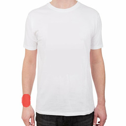
aw/o prog. shrink
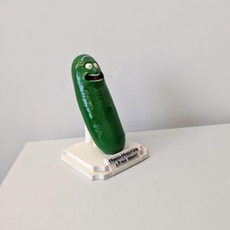
awith prog. shrink

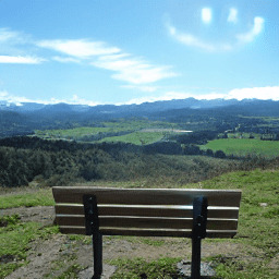
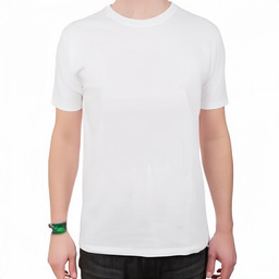
Figure 7. Progressive mask shrinking: With the thin input masks in these examples (first row), the method described in Algorithm 1 fails to alter the image according to the text (second row). This issue is mitigated using progressive mask shrinking (third row).

4.4. Prediction Ranking

Due to the stochastic nature of the diffusion process, we can generate multiple predictions for the same inputs, which is desirable because of the one-to-many nature of our problem. As in previous works (Razavi et al., 2019; Ramesh et al., 2021; Avrahami et al., 2022b), we found it beneficial to generate multiple predictions, rank them, and retrieve the best ones. We rank the predictions by the normalized cosine distance between their CLIP embeddings and the CLIP embedding of the guiding prompt $d$. We also use the same ranking for all of the baselines that we compare our method against, except PaintByWord++ (Bau et al., 2021; Crowson et al., 2022), as it produces a single output per input, and thus no ranking is required.

a	A Input + mask
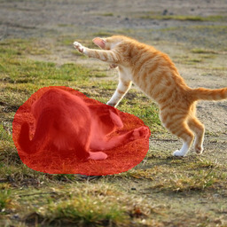
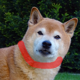
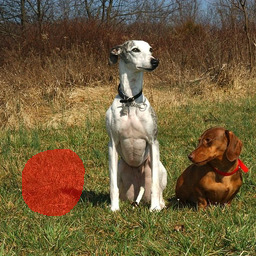
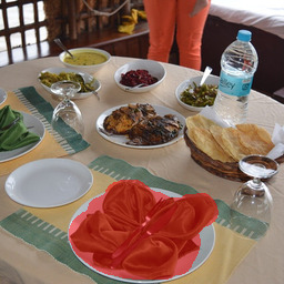
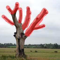
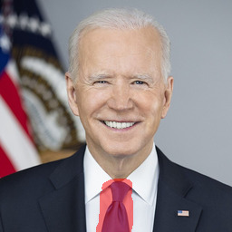
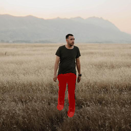
AALocal CLIP-	guided diffusion
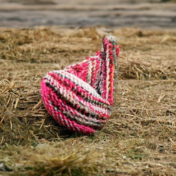
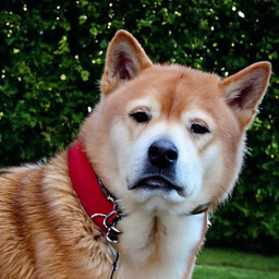
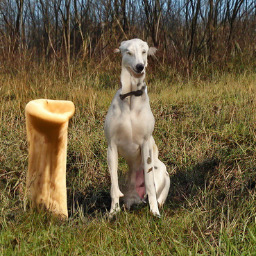
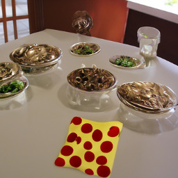
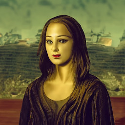
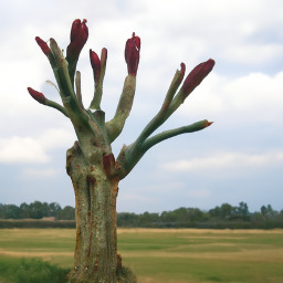
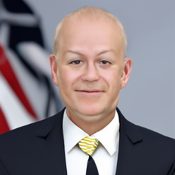
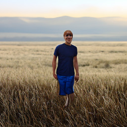
A	PaintByWord++
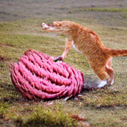
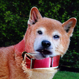
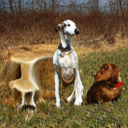
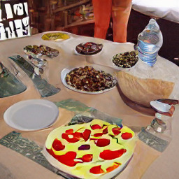
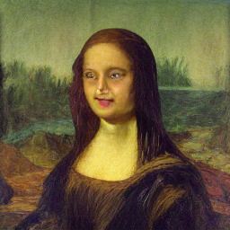
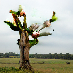
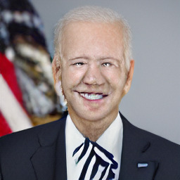
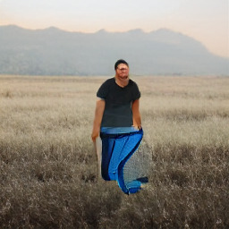
AABlended	AADiffusion
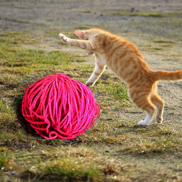
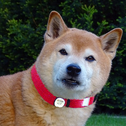
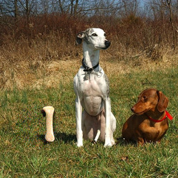
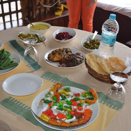
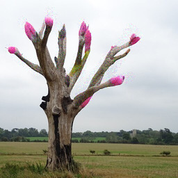
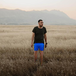
A	AAAGLIDE
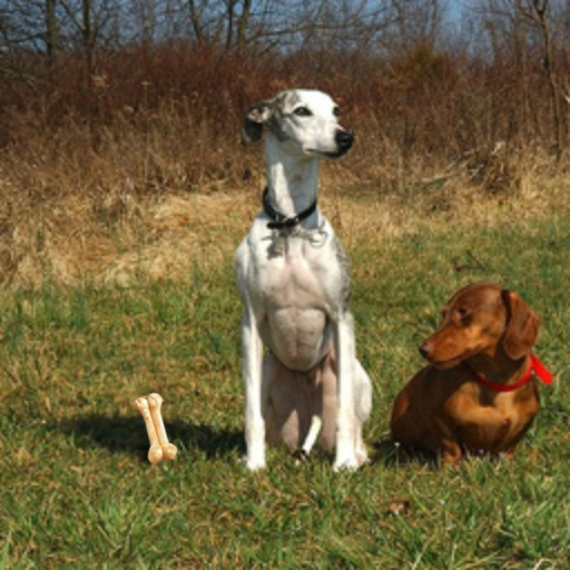
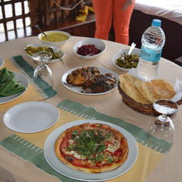
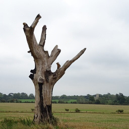
A	aGLIDE-masked
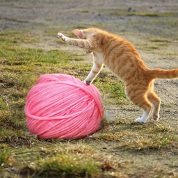
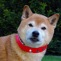
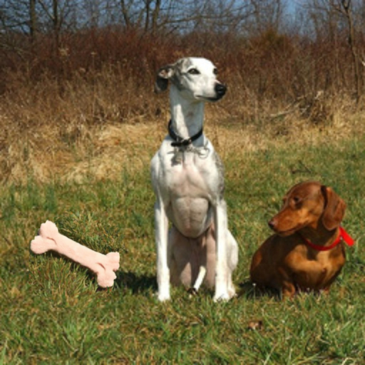
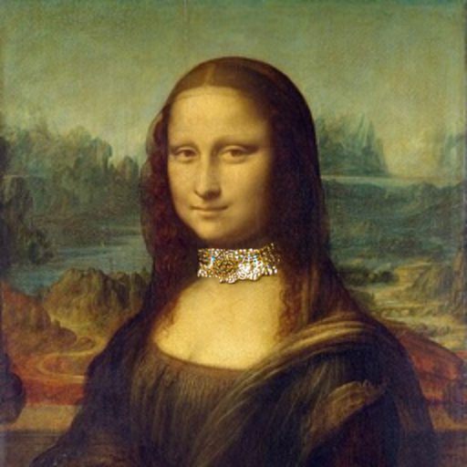
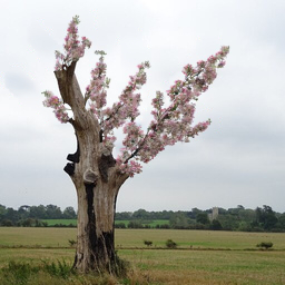
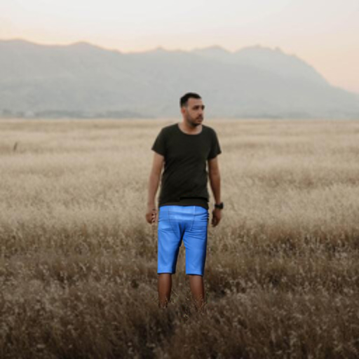
A	aGLIDE-filtered
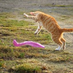
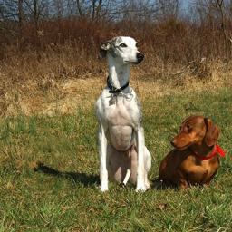
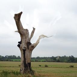
A	AADALL$\cdot$E 2
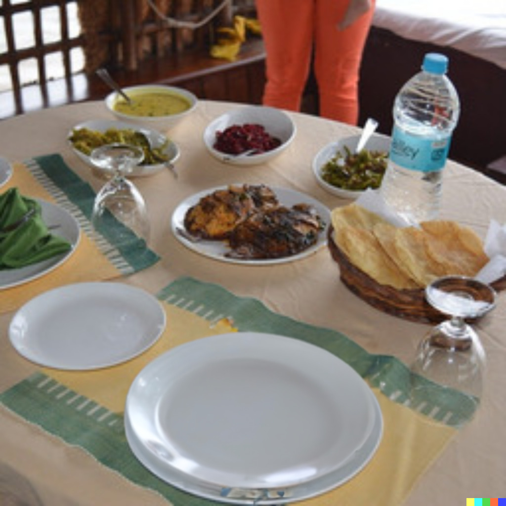
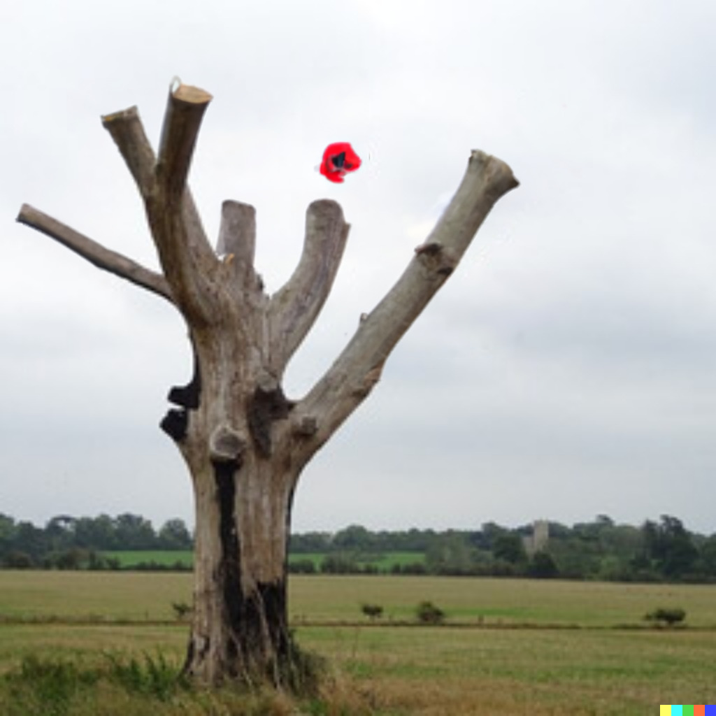
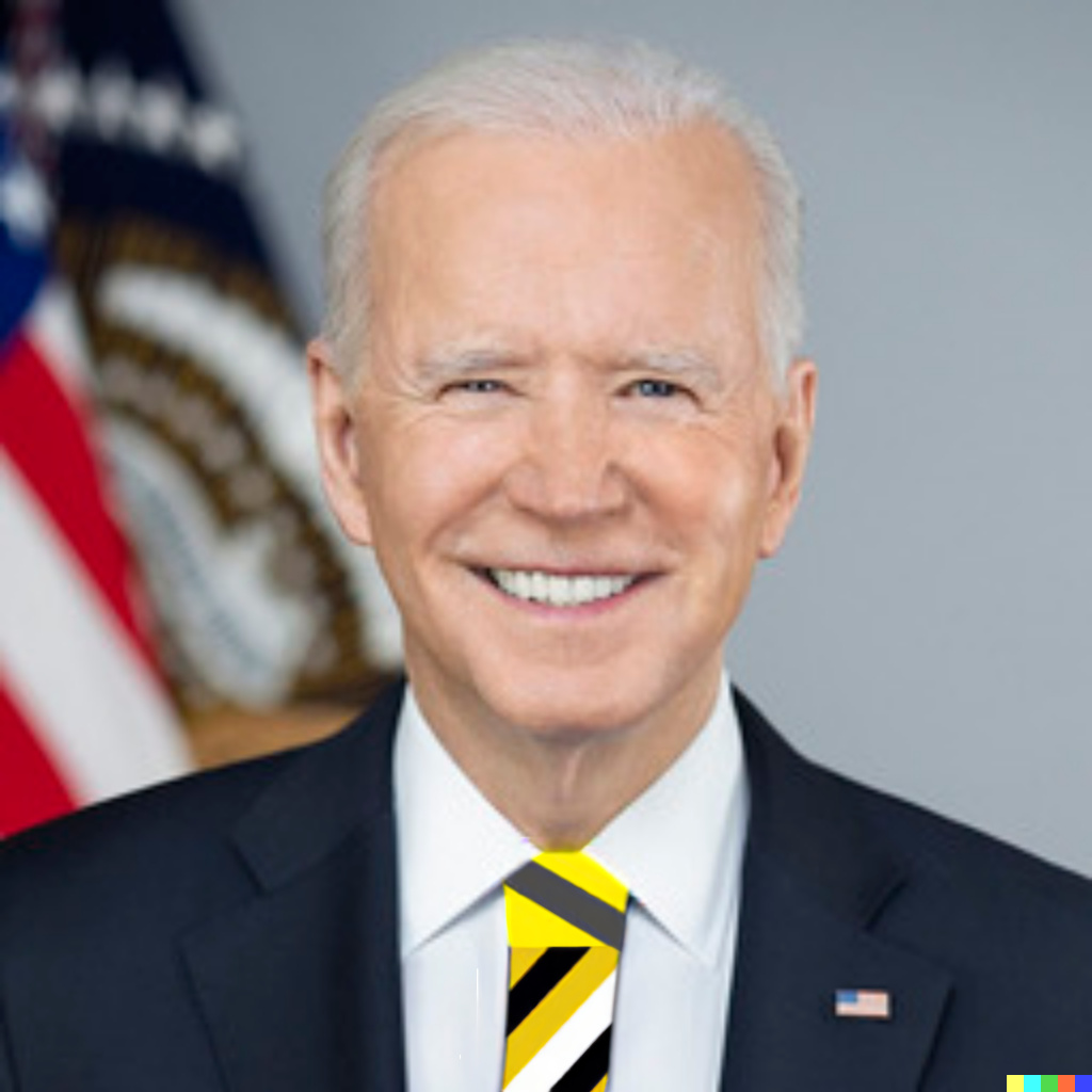
A	AAAOurs
		“pink yarn ball”	“red dog collar”	“dog bone”	“pizza”	“golden	“blooming tree”	“tie with black	“blue short
						necklace”		and yellow	pants”
								stripes”

Figure 8. Comparison to baselines: A comparison with Local CLIP-guided diffusion (Crowson, 2021), PaintByWord++ (Bau et al., 2021; Crowson et al., 2022), Blended Diffusion (Avrahami et al., 2022b), GLIDE (Nichol et al., 2021), GLIDE-masked (Nichol et al., 2021), GLIDE-filtered (Nichol et al., 2021) and DALL$\cdot$E 2 (Ramesh et al., 2022).

5. Results

We begin by comparing our method against previous methods, both qualitatively and quantitatively. Next, we demonstrate several of the use cases enabled by our method.

5.1. Comparisons

In Figure 8 we compare the zero-shot text-driven image editing results produced by our method against the following baselines: (1) Local CLIP-guided diffusion (Crowson, 2021), (2) PaintByWord++ (Bau et al., 2021; Crowson et al., 2022), (3) Blended Diffusion (Avrahami et al., 2022b), (4) GLIDE (Nichol et al., 2021), (5) GLIDE-masked (Nichol et al., 2021), (6) GLIDE-filtered (Nichol et al., 2021), and (7) DALL$\cdot$E 2. See Avrahami et al. (2022b) for more details on baselines (1)–(3). The images for the baselines (1)–(5) were taken directly from the corresponding papers. Note that Nichol et al. (2021) only released GLIDE-filtered, a smaller version of GLIDE, which was trained on a filtered dataset, and this is the only public version of GLIDE. Because the (4) full GLIDE model and (5) GLIDE-masked are not available, we use the results from the paper (Nichol et al., 2021). The images for (3)–(6) and our method required generating a batch of samples and taking the best one ranked by CLIP. The GLIDE model has about $\times 3$ the parameters vs. our model. See the supplementary materials for more details.

Figure 8 demonstrates that baselines (1) and (2) do not always preserve the background of the input image. The edits by GLIDE-filtered (6) typically fail to follow the guiding text. So the comparable baselines are (3) Blended Diffusion, (4) GLIDE, (5) GLIDE-masked, and (7) DALL$\cdot$E 2. As we can see, our method avoids the pixel-level noises of Blended Diffusion (e.g., the pizza example) and generates better colors and textures (e.g., the dog collar example). Comparing to GLIDE, we see that in some cases GLIDE generates better shadows than our method (e.g., the cat example), however it can add artifacts (e.g., the front right paw of the cat in GLIDE’s prediction). Furthermore, GLIDE’s generated results do not always follow the guiding text (e.g., the golden necklace and blooming tree examples), hence, the authors of GLIDE propose GLIDE-masked, a version of GLIDE that does not take into account the given image — by fully masking the context. Using this approach, they manage to generate in the masked area, but it comes at the expense of the transition quality between the masked region and the background (e.g., the plate in the pizza example and the bone in the dogs example). Our method is able to generate a result that corresponds to the text in all the examples, while being blended into the scene seamlessly.

Inspecting DALL$\cdot$E 2 results, we see that most of the results either ignore the guiding text (e.g., the dog collar, dog bone, and pizza examples) or only partially follow it (e.g., “golden necklace” generates a regular necklace, “blooming tree” generates a flower, and “blue short pants” generates text on top of the pants). For more examples, please see the supplementary material.

AAAa“iPod”
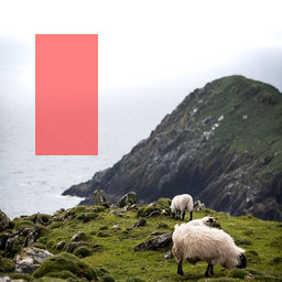
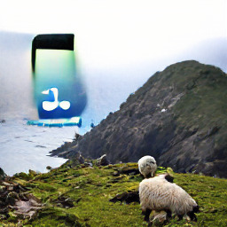
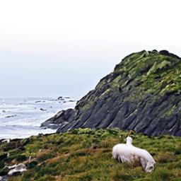
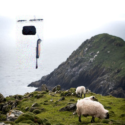
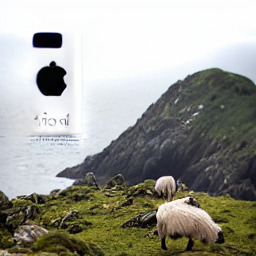
AAa“hourglass”
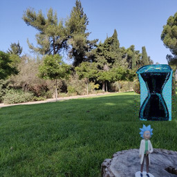
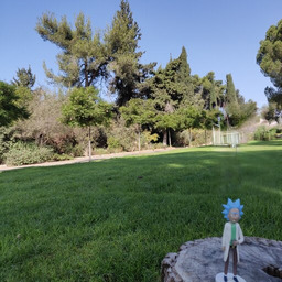
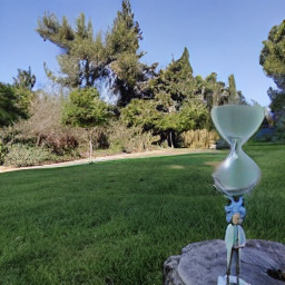
	Input image	Input mask	PaintByWord++	Local CLIP-guided	Blended Diffusion	GLIDE-filtered	Ours
				diffusion

Figure 9. Precision & Diversity Experiment: Two examples of random input images and masks, and the corresponding results of different methods, used in our quantitative evaluation. GLIDE-filtered (Nichol et al., 2021) typically fails to modify the image according to the guiding text prompt; hence, the typical result looks similar to the input image, and therefore looks natural. For more examples please refer to the supplementary material.

During our experiments, we noticed that the predictions of our method typically contain more results that comply with the guiding text prompt. In order to verify this quantitatively, we generated editing predictions for 50 random images, random masks, and text prompts randomly chosen from ImageNet classes. See Figure 9 for some examples. Then, batch precision was evaluated using an off-the-shelf ImageNet classifier. We refrained from using CLIP cosine similarity as the precision measure, because it was shown that CLIP operates badly as an evaluator for gradient-based solutions that use CLIP, due to adversarial attacks (Nichol et al., 2021). We denote this measure as the “precision” of the model. For more details see Section C.1 As reported in Table 1, our method indeed outperforms the baselines by a large margin. In addition, we ranked the results in the batch as described in Section 4.4 and calculated the average accuracy by taking only the top image in each batch, to find that our method still outperforms the baselines.

We also assess the average batch diversity, by calculating the pairwise LPIPS (Zhang et al., 2018a) distances between all the masked predictions in the batch that were classified correctly by the classifier. As can be seen in Table 1, our method has the second-best diversity, but it is outperformed by Local CLIP-guided diffusion by a large margin, which we attribute to the fact that this method changes the entire image (does not preserve the background) and thus the content generated in the masked area is much less constrained.

In addition, we conducted a user study on Amazon Mechanical Turk (AMT) (Amazon, 2022) to assess the visual quality and text-matching of our results. Each of the 50 random predictions that were used in the quantitative evaluation was presented to a human evaluator next to a result from one of the baselines. The evaluator was asked to choose which of the two results has a better (1) visual quality and (2) matches the text more closely. The evaluators could also indicate that neither image is better than the other. As seen in Table 1 (right), the majority ($\geq 50\%$) of evaluators prefer the visual quality and the text matching of our method over the other methods. A binomial statistical significance test, reported in Table 2 in the supplementary material, suggests that these results are statistically significant. The results of GLIDE-filtered (Nichol et al., 2021) were preferred in terms of visual quality, however these results typically fail to change the input image or make negligible changes: thus, although the result looks natural, it does not reflect the desired edit. See Figure 9 and the supplementary material for more examples and details. We chose to use a two-way question system in order to make the task clearer to the evaluators by providing only two images without the input image and mask.

Table 1. Quantitative comparison. In terms of precision, our method outperforms the baselines, both at the batch level and at the best result level. In terms of diversity, only the Local CLIP-guided diffusion baseline achieves a better score, due to its tendency to change the entire image significantly (lack of background preservation). The two rightmost columns report the percentage of human evaluators that preferred our method over the baseline. Our method outperforms the baselines in terms of visual quality and text matching except the visual quality of GLIDE-filtered, which mostly leaves the input untouched.

Method Batch Batch Best Result Human Human Precision $\uparrow$ Diversity $\uparrow$ Precision $\uparrow$ Vis. Quality Text Matching Blended Diffusion 10.4% 0.106 36% 64% 55% Local CLIP-guided diffusion 10.49% 0.419 38% 74% 62% PaintByWord++ - - 0% 94% 68% GLIDE-filtered 1.87% 0.114 4% 26% 86% Ours 28.66% 0.115 54% - -

5.2. Inference Time Comparison

Table 2. Inference time comparison: Our method outperforms all other methods when using batch processing. This stems from the fact that we perform diffusion in the latent space, and because our background preservation optimization is only required for the top-ranked result. Batch sizes marked with $*$ are below the size recommended by the respective authors (lower batch precision), but are reported for comparison purposes.

Method Batch Single Image Full Batch Per Image in Size (sec) $\downarrow$ (sec) $\downarrow$ Batch (sec) $\downarrow$ Blended Diffusion 64 27 1472 23 Blended Diffusion $24^{*}$ 27 552 23 Local CLIP-guided diffusion 64 27 1472 23 Local CLIP-guided diffusion $24^{*}$ 27 552 23 PaintByWord++ - 78 - - GLIDE-filtered 24 7 89 3.7 Ours (without background opt.) 24 6 53 2.2 Ours (with background opt.) 24 25 72 3

We compare the inference time of various methods on an A10 NVIDIA GPU in Table 2. We show results for Blended Diffusion and GLIDE-filtered (the available smaller model, which is probably faster than the full unpublished model). Both of these methods require generating multiple predictions (batch) and taking the best one in order to achieve good results. The recommended batch size for Blended Diffusion is 64, whereas GLIDE-filtered and our method use a batch size of 24.

Our method supports generation with or without optimizing for background preservation (Section 4.2), and we report both options in Table 2. The background optimization introduces an additional inference time overhead, however, it is up to the user to decide whether this additional step is necessary (e.g., when editing images with human faces). Our method outperforms the baselines on the standard case of batch inference, even when accounting for the background preservation optimization. The acceleration in comparison to Blended Diffusion and Local CLIP-guided diffusion is $\times 10$ with equal batch sizes and $\times 20$ with the recommended batch sizes, which stems from the fact that our generation process is done in the lower dimensional latent space, and the background preservation optimization need only be done on the selected result. The acceleration in comparison to PaintByWord++ and GLIDE-filtered is $\times 1.47$ and $\times 1.23$, respectively.

5.3. Use Cases

Our method is applicable in a variety of editing scenarios with generic real-world images, several of which we demonstrate here.

Text-driven object editing: using our method one can easily add new objects (Figure 1(top left)) or modify or replace existing ones (Figure 1(top right)), guided by a text prompt. In addition, we have found that the method is capable of injecting visually plausible text into images, as demonstrated in Figure 1(middle left).

Background replacement: rather than inserting or editing the foreground object, another important use case is text-guided background replacement, as demonstrated in Figure 1(middle right).

Scribble-guided editing: The user can scribble a rough shape on a background image, provide a mask (covering the scribble) to indicate the area that is allowed to change, and provide a text prompt. Our method transforms the scribble into a natural object while attempting to match the prompt, as demonstrated in Figure 1(bottom left).

For all of the use cases mentioned above, our method is inherently capable of generating multiple predictions for the same input, as discussed in Section 4.4 and demonstrated in Figure 1(bottom right). Due to the one-to-many nature of the task, we believe it is desirable to present the user with ranked (Section 4.4) multiple outcomes, from which they may chose the one that best suits their needs. Alternatively, the highest ranked result can be chosen automatically. For more results, see Section A in the supplementary.

6. Limitations & Conclusions

a“a man with a	aared suit”
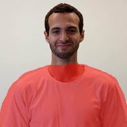
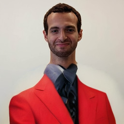
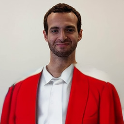
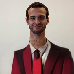
a	a“big mountain”
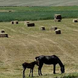
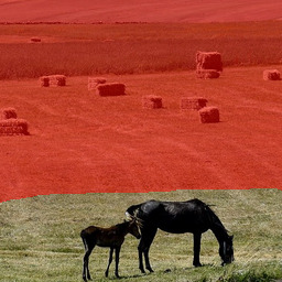
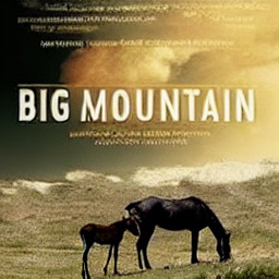
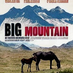
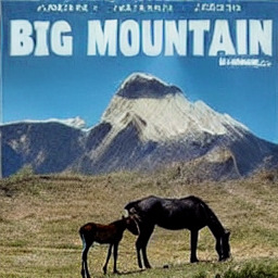
		Input image	Input mask

Figure 10. Limitations: Top row: our CLIP-based ranking takes into account only the masked area, Thus, the results are sometimes only piece-wise realistic, and the image does not look realistic as a whole. Bottom row: the model has a text bias - it may try to create movie posters/book covers with text instead or in addition to generating the actual object.

Prompt sen.
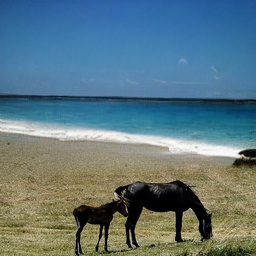
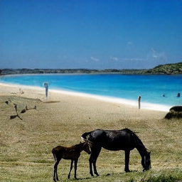
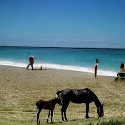
	input + mask	“a beach!”	“beaches”	“a day at
				the beach”
Mask sen.
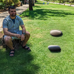
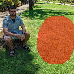
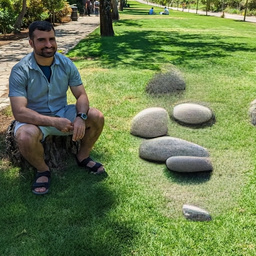
	small mask	“stones”	big mask	“stones”
Image sen.
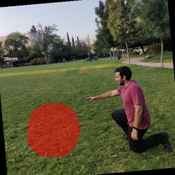
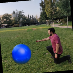
	original image	“a blue ball”	rotated image	“a blue ball”

Figure 11. Sensitivity analysis: we found our method to be somewhat sensitive to its inputs. Small changes to the input prompt (first row), to the input mask (second row), or to the input image (third row) may result in small output changes.

Although our method is significantly faster than prior works, it still takes over a minute on an A10 GPU to generate a ranked batch of predictions, due to the diffusion process. This limits the applicability of our method on lower-end devices. Hence, accelerating the inference time further is still an important research avenue.

As in Blended Diffusion, the CLIP-based ranking only takes into account the generated masked area. Without a more holistic view of the image, this ranking ignores the overall realism of the output image, which may result in images where each area is realistic, but the image does not look realistic overall, e.g., Figure 10(top). Thus, a better ranking system would prove useful.

Furthermore, we observe that LDM’s amazing ability to generate texts is a double-edged sword: the guiding text may be interpreted by the model as a text generation task. For example, Figure 10(bottom) demonstrates that instead of generating a big mountain, the model tries to generate a movie poster named “big mountain”.

In addition, we found our method to be somewhat sensitive to its inputs. Figure 11 demonstrates that small changes to the input prompt, to the input mask, or to the input image may result in small output changes. For more examples and details, please read Section D in the supplementary material.

Even without solving the aforementioned open problems, we have shown that our system can be used to locally edit images using text. Our results are realistic enough for real-world editing scenarios, and we are excited to see what users will create with the source code that we will release upon publication.

Appendix A Additional Examples

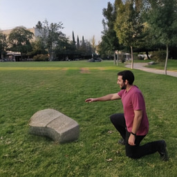
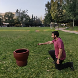
“big stone”	“bowl of water”	“bread”	“Buddha”	“car tire”	“clay pot”
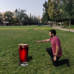
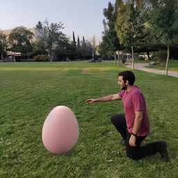
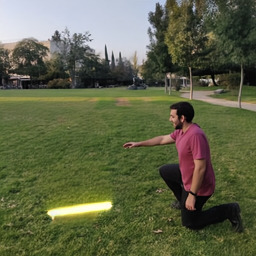
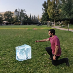
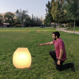
“cola”	“egg”	“glow stick”	“ice cube”	“lamp”	“milk”
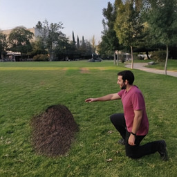
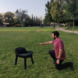
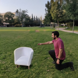
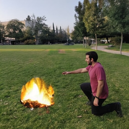
“pile of dirt”	“pile of gold”	“tooth”	“black chair”	“white chair”	“bonfire”
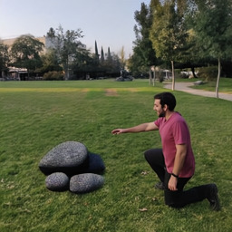
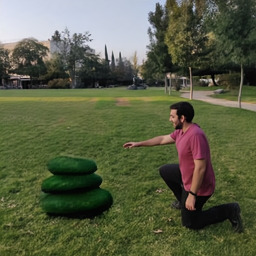
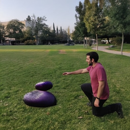
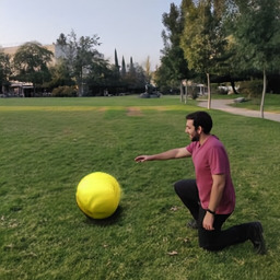
“stones”	“black stones”	“green stones”	“purple stones”	“red ball”	“yellow ball”
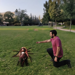
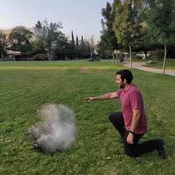
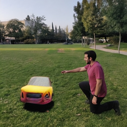
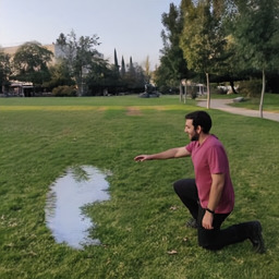
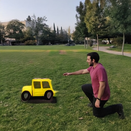
“huge ant”	“smoke”	“toy car”	“water puddle”	“huge apple”	“yellow toy truck”

Figure 12. Adding a new object: Additional examples for adding a new object within a scene.

“N” AAa text “GAN”
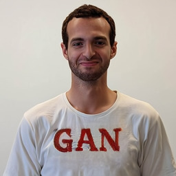
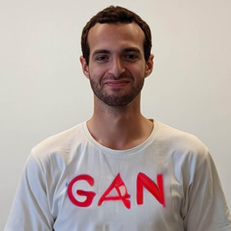
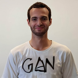
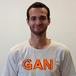
graffiti with the text “No Free Lunch”
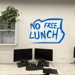
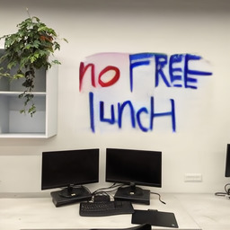
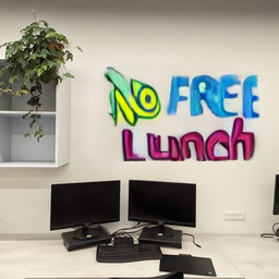
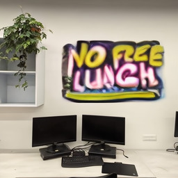
“N” A “big mountain”
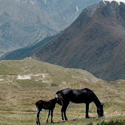
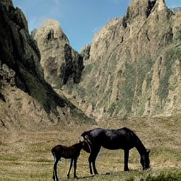
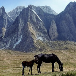
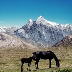
“N” A “colorful balls”
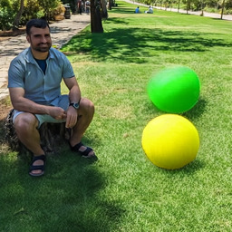
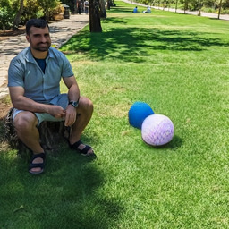
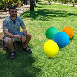
“N” AAa “ice cube”
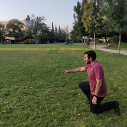
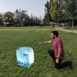
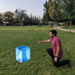
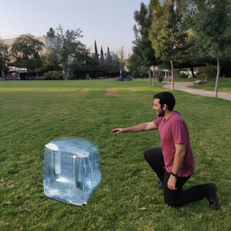
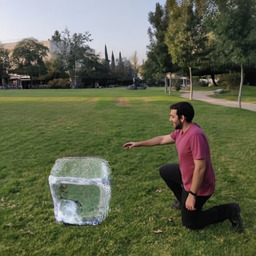
	Input image	Input mask	Prediction 1	Prediction 2	Prediction 3	Prediction 4

Figure 13. Multiple predictions: Dealing with a one-to-many task, there is a need to generate multiple predictions.

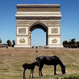
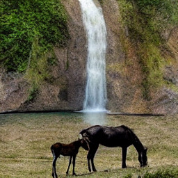
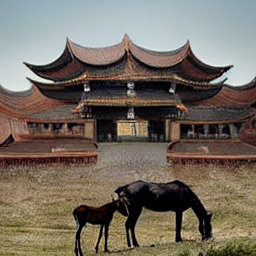
Input image	Input mask	“Acropolis”	“Arc de Triomphe”	“big waterfall”	“China”
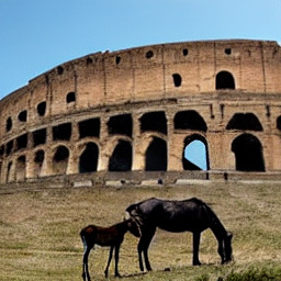
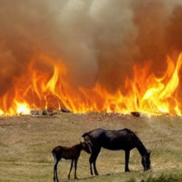
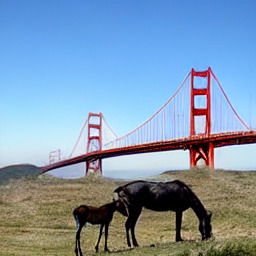
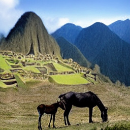
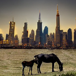
“Colosseum”	“fire”	“Golden Gate Bridge”	“Machu Picchu”	“Mount Fuji”	“New York City”
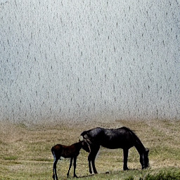
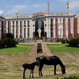
“nuclear power plant”	“Petra”	“rainy”	“river”	“Stanford University”	“Stonehenge”
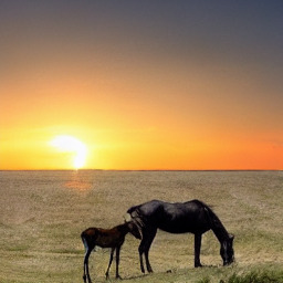
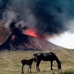
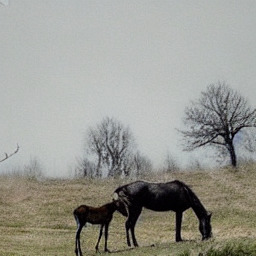
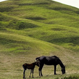
“sunny”	“sunrise”	“swimming pool”	“volcanic eruption”	“winter”	“green hills”
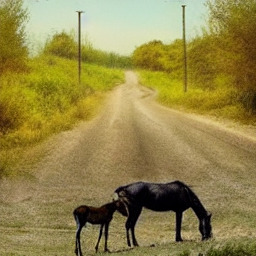
“desert”	“big lake”	“forest”	“dusty road”	“horses stable”	“houses”

Figure 14. Replacing the background: Additional examples for the background replacement capability of our model.

	AAAA“stones”
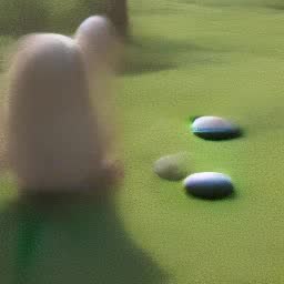
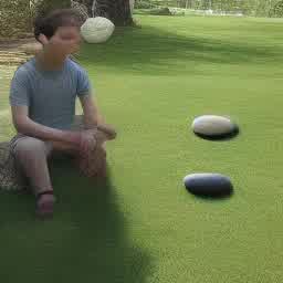
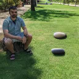
	AAa“a blue ball”
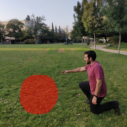
	AAA“a beach”
AA“a man with a	AAAgreen shirt”
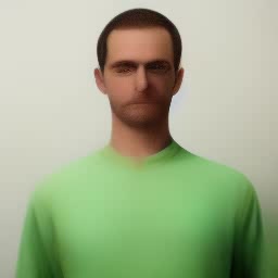
AAA“an avocado	AAAApainting”
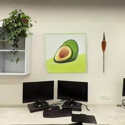
		input + mask		diffusion start				diffusion end

Figure 15. Process visualization: a visualization of the diffusion process for various inputs, without the background reconstruction step that is explained in section 4.2 in the main paper.

AAAA “white clouds”
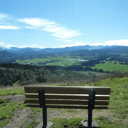
AAAA “green smoke”
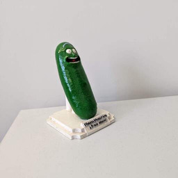
AAAAAAAA “fire”
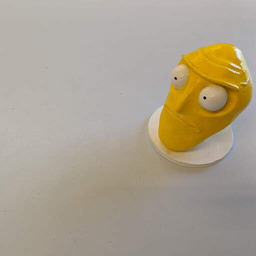
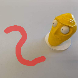
AAAAA “green bracelet”
	Input image	Input mask	Standard process	Progressive mask shrinking

Figure 16. Thin masks: An expanded version of Figure 6 from the main paper .

In Figure 12 we demonstrate more examples of adding a new object to a scene. In Figure 13 we demonstrate the one-to-many generation ability of our model. In Figure 14 we demonstrate more examples of background replacement. In addition, in Figure 15 we provide a visualization of the diffusion process on several examples.

A.1. Interactive Editing

Step 1: “a man with a green sweater”
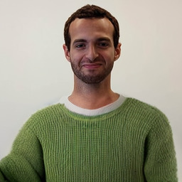
AAAAAAStep 2: “a straw hat”
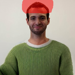
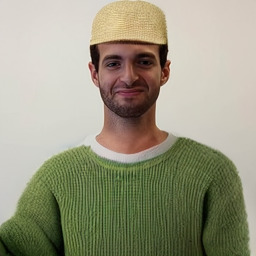
AAAAAAStep 3: “a window”
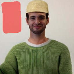
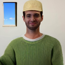
Input image	Input mask	Prediction

Figure 17. Editing session: The user is able to perform several edit operations consecutively. First, the user provides the input image, mask, and text prompt “a man with a green sweater” to get the first result, then, he masks the head area and provides the text prompt “a straw hat”, finally, he masks an area on the wall and provides the text “a window” to get the final result.

Because of the near-perfect background preservation of our method, the user is able to perform an interactive editing session: editing the image gradually, where at each stage of the editing session the user edits a different area within the image without changing the other parts of the image that were already edited. We show an interactive editing session in Figure 17.

Appendix B Additional Comparisons

In this section we start by comparing the number of parameters of our model against the baselines, discuss pixel-level artifacts of Blended Diffusion, show additional visual comparisons to the baselines, and compare against a variant of the background reconstruction loss.

B.1. Parameters Comparison

In Table 3 we compare the number of parameters in our model to that of the following baselines: (1) Local CLIP-guided diffusion (Crowson, 2021) (for more details see Avrahami et al. (2022b)), (2) PaintByWord++ (Bau et al., 2021; Crowson et al., 2022) (for more details see Avrahami et al. (2022b)), (3) Blended Diffusion (Avrahami et al., 2022b), (4) GLIDE (Nichol et al., 2021) and (5) GLIDE-filtered (Nichol et al., 2021).

Table 3. Parameters comparison: A comparison between the number of parameters of the different models. We used the same CLIP model for all the base models which has 0.15B parameters.

Method	# Parameters
Local CLIP-guided diffusion	0.55B + 0.15B = 0.70B
PaintByWord++	0.09B + 0.15B = 0.24B
Blended Diffusion	0.55B + 0.15B = 0.70B
GLIDE	5.00B + 0.15B = 5.15B
GLIDE-filtered	0.30B + 0.15B = 0.45B
Ours	1.45B + 0.15B = 1.60B

B.2. Pixel-level Artifacts Comparison

As described in Section 4 of the main paper, the latent space diffusion used by our method is not only faster than pixel-based diffusion, but also mitigates the pixel-level artifacts in Blended Diffusion (Avrahami et al., 2022b). We provide additional comparisons in Figure 18.

A	AAAA“blue ball”
A	AAAA“knit beanie”
A	AAAAAA“pizza”
A	AAA“corgi painting”
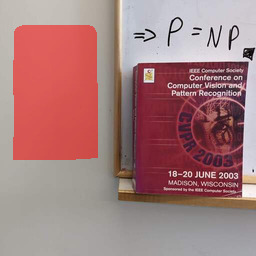
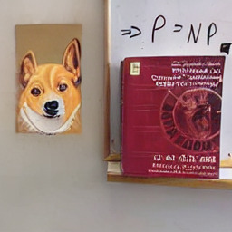
A	AAAAA“cucumber”
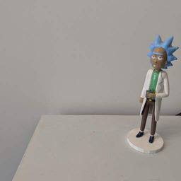
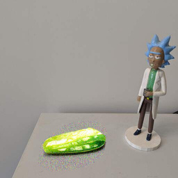
AAAA“a man with	AAAa yellow sweater”
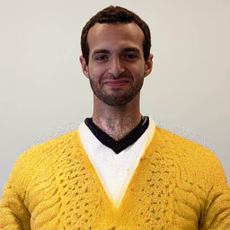
		(a) Input image	(b) Input mask	(c) Blended Diffusion	(d) Ours

Figure 18. Noise artifacts: Given the input image (a) and mask (b) with some guiding text, Blended Diffusion produces noticeable pixel-level noise artifacts (c), in contrast to our method (d).

B.3. Additional Comparison Against the Baselines

In Figure 7 in the main paper, we compared our method against the baselines qualitatively on the set of images provided by Blended Diffusion (Avrahami et al., 2022b). In addition, we compare our method against the freely-available models in Figure 19.

As we can see, baselines (1) Local CLIP-guided diffusion and (2) PaintByWord++ fail to preserve the background of the input image. Baseline (4) GLIDE-filtered does not follow the guiding text, whereas (5) DALL$\cdot$E 2 only partially corresponds to the guiding text (in the corgi and the yellow sweater examples). While (3) Blended Diffusion does preserve the background and follows all of the input guiding texts (except for the graffiti example), it suffers from noise-level artifacts as described in Section B.2.

A	AA Input + mask
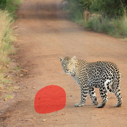
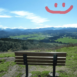
AAALocal CLIP-	AAguided diffusion
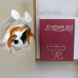
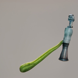
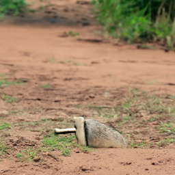
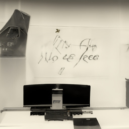
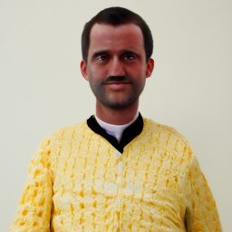
A	AAPaintByWord++
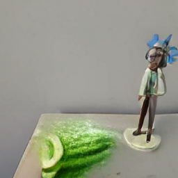
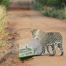
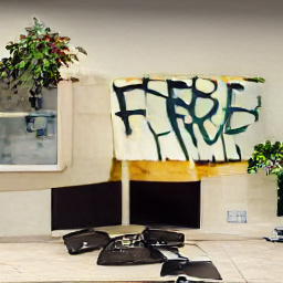
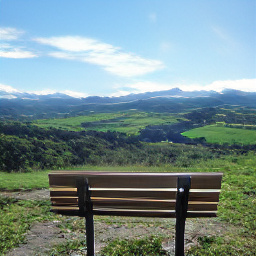
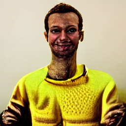
A	ABlended Diffusion
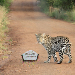
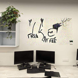
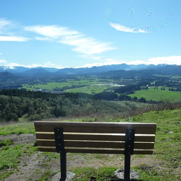
A	AAaGLIDE-filtered
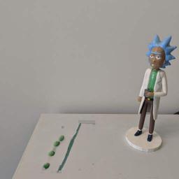
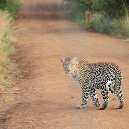
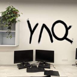
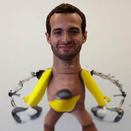
A	AAAaDALL$\cdot$E 2
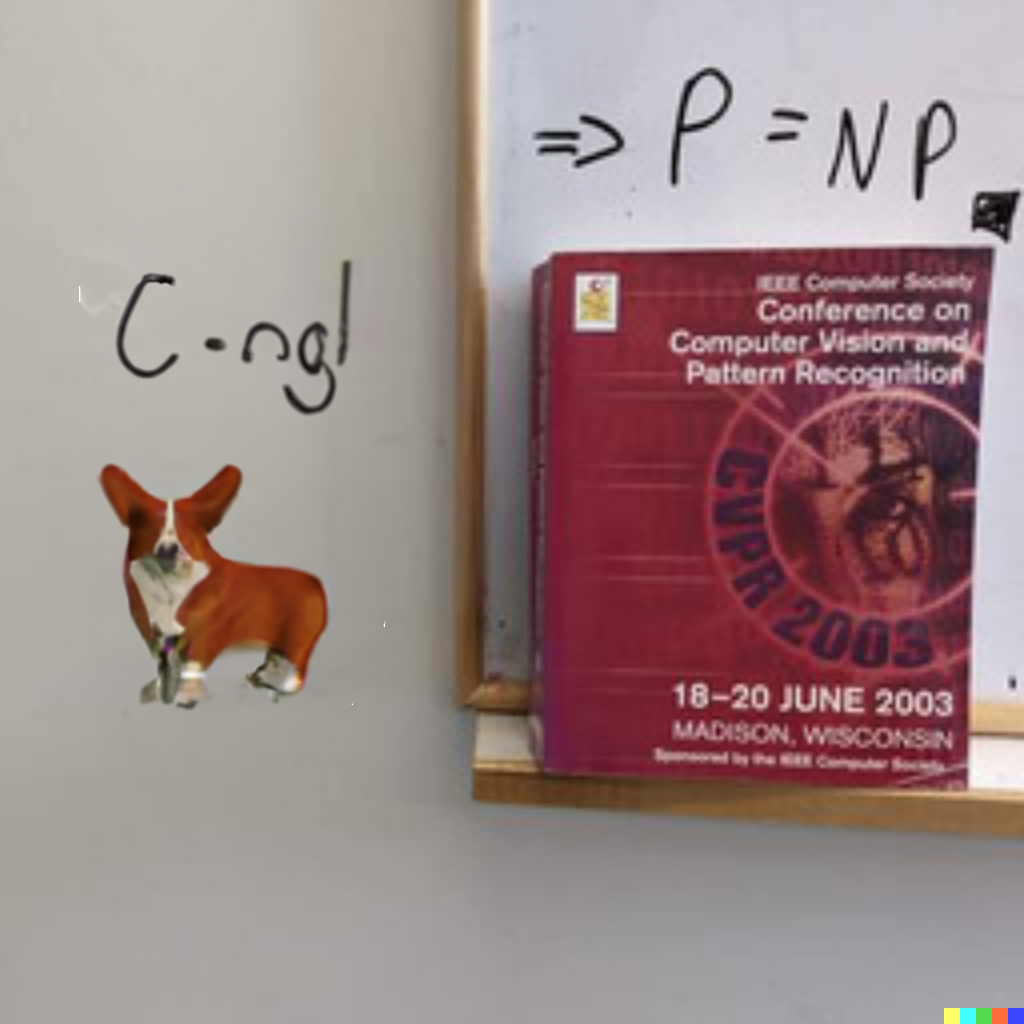
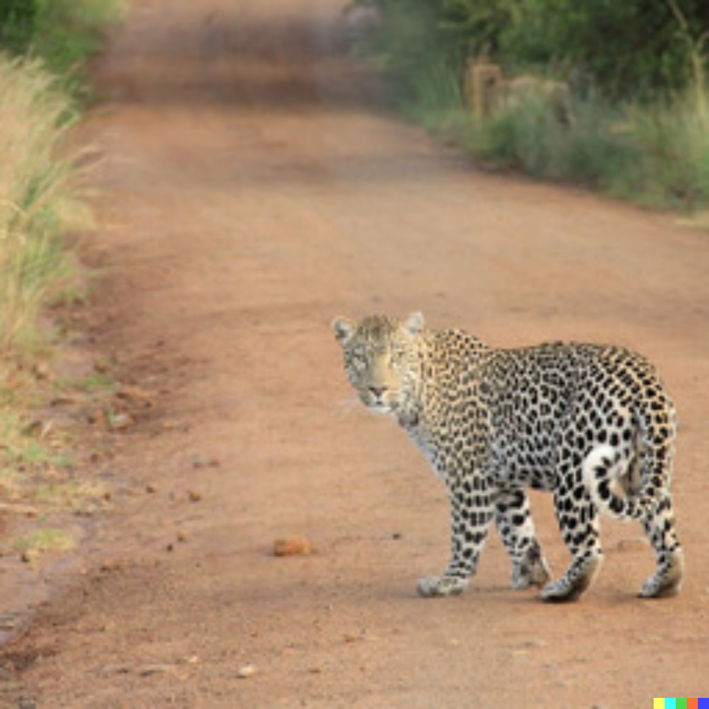
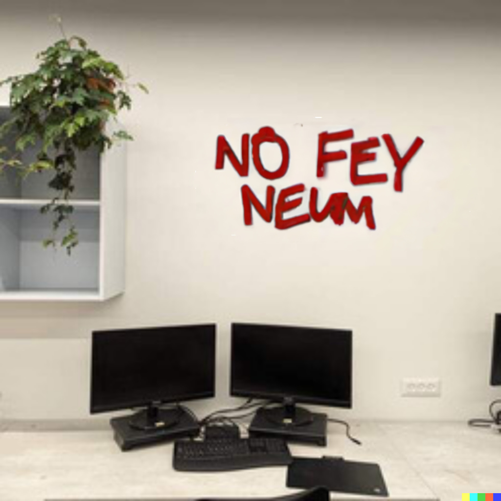
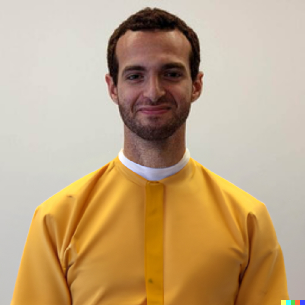
A	AAAAAOurs
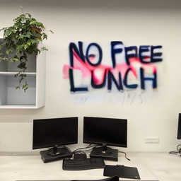
		“corgi painting”	“cucumber”	“gravestone”	“graffiti with the text	“white clouds”	“a man with a
					‘No Free Lunch’ ”		yellow sweater”

Figure 19. Comparison to baselines: A comparison with Local CLIP-guided diffusion (Crowson, 2021), PaintByWord++ (Bau et al., 2021; Crowson et al., 2022), Blended Diffusion (Avrahami et al., 2022b), GLIDE-filtered (Nichol et al., 2021) and DALL$\cdot$E 2 (Ramesh et al., 2022).

B.4. Background Reconstruction Loss Comparison

As described in Section 4.2 we handled the background reconstruction by optimizing the decoder’s weights $\theta$ on a per-image basis:

(3) $$\theta^{*}=\operatornamewithlimits{argmin}\limits_{\theta}\|D_{\theta}(z_{0})\odot m-\hat{x}\odot m\|\;$$

λ∥Dθ(z0)⊙(1-m)-x⊙(1-m)∥

where $D_{\theta}$ is the decoder, $m$ is the input mask, $x$ is the input image and $\hat{x}$ is the predicted image. Because our goal is to preserve the background, we set most of the weight to the background term (by setting $\lambda=100$). It raises the question of what is the effect of dropping the foreground term completely. As demonstrated in Figure 20, doing so makes the colors of the edited area less vivid.

AAAAA“red hair”
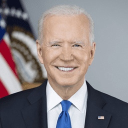
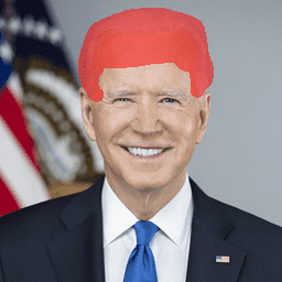
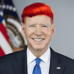
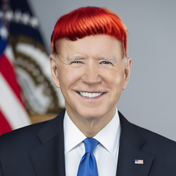
AAA“colorful balls”
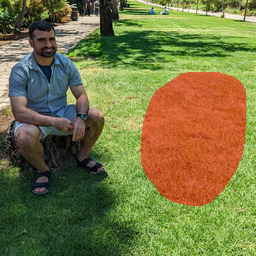
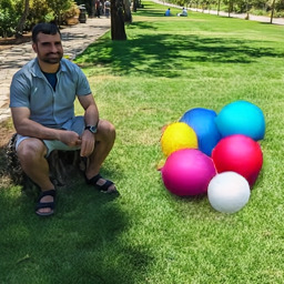
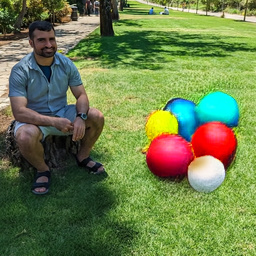
AAA“purple stones”
		input + mask	with foreground term	without foreground term

Figure 20. Reconstruction loss ablation: Removing the foreground term in Equation 3 results in slightly less vivid colors.

Appendix C Implementation Details

For all the experiments reported in this paper, the pretrained models that we have used are:

• Text-to-image Latent Diffusion model published by Rombach et al. (2022).

• CLIP model with ViT-B/16 backbone for the Vision Transformer (Dosovitskiy et al., 2020), as released by Radford et al. (2021).

• Blended Diffusion model from Avrahami et al. (2022b).

• GLIDE-filtered model from Nichol et al. (2021).

All these methods were released under MIT license and were implemented using PyTorch (Paszke et al., 2019).

In addition, we used the online demo of DALL$\cdot$E 2 (OpenAI, 2022b) which enables the user to manually edit a real image using its interface. Nevertheless, the usage of the system is free for only a limited number of credit tokens, and the model is not available. Hence, we could not calculate our precision and diversity metrics on this model.

All the input images in this paper are real images that were released freely under a Creative Commons license or from our private collection.

In the reconstruction methods described in Section 4.2 we used the following:

• For Poisson image blending (Pérez et al., 2003) we used the OpenCV (Bradski and Kaehler, 2000) implementation.

• For latent optimization and weights optimization we used Adam optimizer (Kingma and Ba, 2014) with a learning rate of 0.0001 for 75 optimization steps per image.

For the progressive mask shrinking described in Section 4.3 we used the following scheme: we dilate the downsampled mask $m_{\textit{latent}}$ with kernels of ones with sizes $3\times 3$, $5\times 5$ and $7\times 7$, then we divide the diffusion process into four parts with the same number of steps in each part, with the first part using the most dilated mask, and the last part using the original mask.

C.1. Precision & Diversity Metrics

As described in Section 5 we calculated precision and diversity metrics in order to compare our method against the baselines quantitatively. As was shown by Nichol et al. (2021), using CLIP model as an evaluator for text correspondence of images that were edited with models that use CLIP’s gradients for generation, is not correlated with human evaluation, because these models are susceptible to adversarial examples. Hence, because some of our baselines are using CLIP, we had to look for an alternative evaluation model. We opted to use a pre-trained ImageNet classifier, EfficentNet (Tan and Le, 2019), as our backbone.

We took 50 random images from the web and local collection; next, for each image, we generated a random rectangular mask with dimensions that are in the range $[\frac{dim}{5},\frac{dim}{2}]$ where $dim$ is the corresponding image dimension. Then, for each of the resulting image-mask pairs, we sample a random class from ImageNet classes and use the corresponding text label of that class as an input to our model. For each of the baseline models, we generate predictions of the recommended batch size. An example of an input and its predictions by the various baselines can be seen in Figure 21.

AAA“crane”
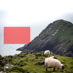
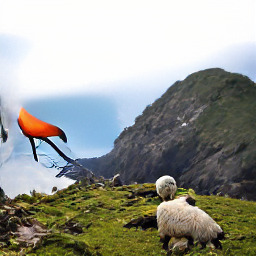
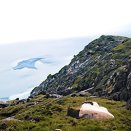
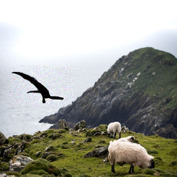
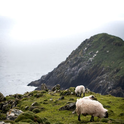
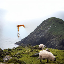
AAAa“iPod”
AAA“hourglass”
AAA“flamingo”
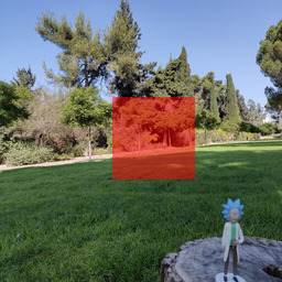
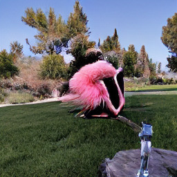
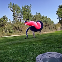
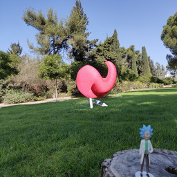
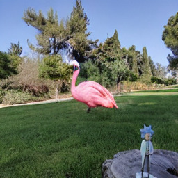
AAa“Chihuahua”
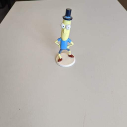
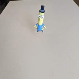
AAa“cockroach”
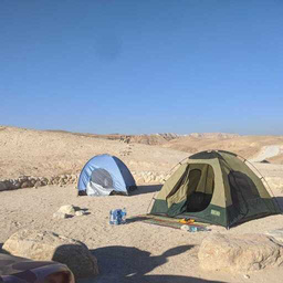
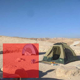
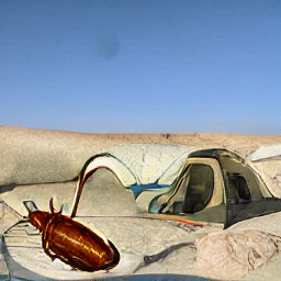
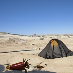
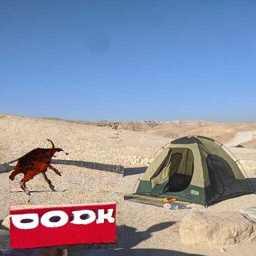
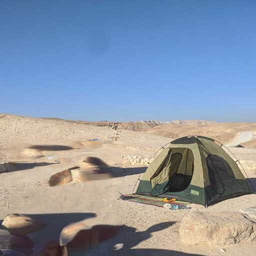
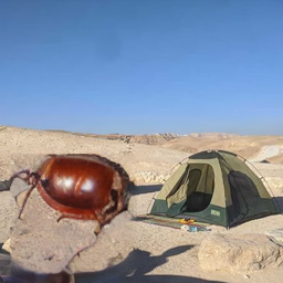
AAA“baloon”
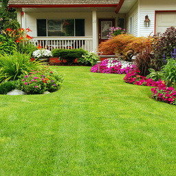
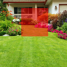
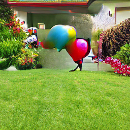
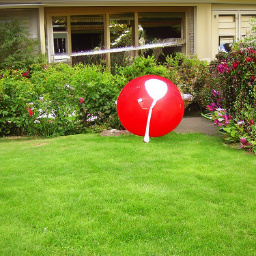
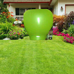
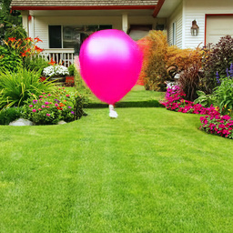
	Input image	Input mask	PaintByWord++	Local CLIP-guided	Blended Diffusion	GLIDE-filtered	Ours
				diffusion

Figure 21. Precision & Diversity Experiment: An example of a random image and mask, and the generated results, used in our quantitative evaluation.

To calculate the precision for each model, we go over all its predictions, mask them using the input mask, and feed the masked results to the ImageNet classifier. Because ImageNet contains many classes with semantically close meaning (e.g., several different species of dogs), we considered prediction as a good prediction if the ground-truth class label (the label of the class that was fed to the generative model) is in the top-5 predictions of the classification model. We calculate the average accuracy at the batch level for each input. In addition, we calculate the precision only on the top result that was ranked by the CLIP model as described in Section 4.4 Both of these metrics are reported in Table 1

In order to calculate the diversity at the batch level, for each input triplet, we take only the images that were classified correctly by the classifier (because only these images are of interest to the end-user). We then mask the images using the corresponding masks, in order to isolate the diversity of the foreground and then calculate the pairwise LPIPS (Zhang et al., 2018a) distance and take the average across all the predictions.

C.2. User Study

As described in Section 5 we conducted a user study in order to assess the visual quality of the results and how well they match the guiding text, using the Amazon Mechanical Turk platform (AMT) (Amazon, 2022). We used the 50 random predictions that were used to evaluate our method quantitatively, as described in Section C.1. We presented each human evaluator with two images — one produced by our method and the other one by a baseline, and asked them to rate which of the two images has (1) better visual quality by asking “Which of the following images has better visual quality?” and (2) better matches the text prompt by asking “Which of the following images matches the label X more closely?” (replacing X with the text prompt). We used the majority vote of the raters for each question. The human raters could also indicate for each question that neither of the images is better than the other (“Equal quality” for the image quality/“Equally match” for the text matching), in which case we split the points between both of the models equally. We collected five ratings per question, resulting in 250 ratings per task (visual quality/text match). The time allotted per image-pair task was one hour, to allow the raters to properly evaluate the results without time pressure.

We included in our user study only the freely available models that could be used with the random predictions, hence, the study does not include the GLIDE-full (Nichol et al., 2021) and DALL$\cdot$E 2 (Ramesh et al., 2022) models, which are unavailable. A binomial statistical significance test, reported in Table 4, suggests that these results are statistically significant.

Table 4. User study statistical analysis. A binomial statistical test of the user study results suggests that our results are statistically significant (p-value ¡ 5%).

Method Visualization Quality Text Matching p-value p-value Blended Diffusion ¡ 0.001 0.043 Local CLIP-guided diffusion ¡ 0.001 ¡ 0.001 PaintByWord++ ¡ 0.001 ¡ 0.001 GLIDE-filtered ¡ 0.001 ¡ 0.001

C.3. Ranking Effectiveness

a AAA“cat painting”
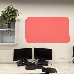
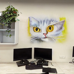
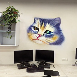
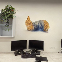
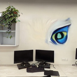
a AAAA“Buddha”
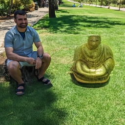
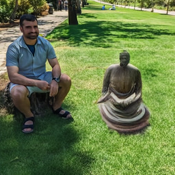
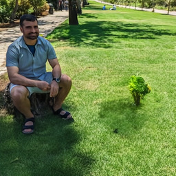
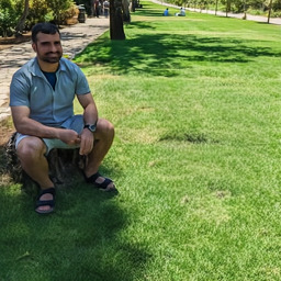
AAaa horror book AAanamed ’CVPR’
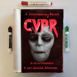
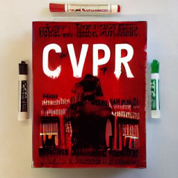
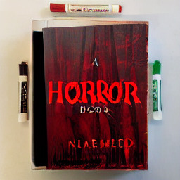
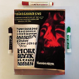
	Input image	Input mask	1st ranked result	2nd ranked result	23th ranked result	24th ranked result

Figure 22. Ranking effectiveness: We generate 24 prediction results and rank them using the CLIP (Radford et al., 2021) model. The top 20% of results are constantly better than the bottom 20%, but not at the granularity of a single image — the first image is not always strictly better than the second.

AAAAA “corgi painting”
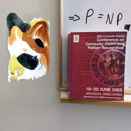
a “a man with a yellow sweater”
AAAAAA “cucumber”
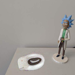
AAAAA “white clouds”
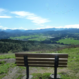
	Input image	Input mask	Without ranking	With ranking

Figure 23. Ranking effectiveness in Blended Diffusion: The CLIP ranking is a crucial part of Blended Diffusion (Avrahami et al., 2022b). When generating a single prediction result, the output rarely corresponds to the input text prompt.

As described in Section 4.4 in the main paper, we utilized the CLIP model in order to rank the predictions of our method. As demonstrated in Figure 22, during our experiments we noticed that the top 20% are constantly better than the bottom 20%, but not at the granularity of a single image — the first image is not always strictly better than the second.

In addition, Figure 23 demonstrates the importance of the CLIP ranking for the Blended Diffusion baseline (Avrahami et al., 2022b). As we can see, the CLIP ranking is essential to this method. Hence, the “full batch” column in Table 2 on the main paper is the relevant information we should take into account when comparing the inference times of our method with those of the Blended Diffusion baseline.

Appendix D Sensitivity Analysis

We found that small input changes to our method may result in small output changes. In Figure 24 we demonstrate how small changes to the input prompt may result in small changes to the output. Furthermore, in Figure 25 we demonstrate that small changes to the input mask (making it larger/smaller) may also change the output result. Lastly, in Figure 26 we performed small input changes: rotating the image by $5\degree$ and performing a blurring by a Gaussian kernel with $\sigma=2$ standard deviation and kernel size $k=8$. As we can see, the outputs may change due to these input changes.

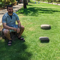
input + mask	“stones”	“some stones”	“stones!”	“many stones”	“stone”
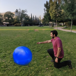
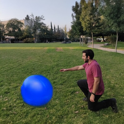
input + mask	“a blue ball”	“a blue ball!”	“a blue ball?”	“a very blue ball”	“blue ball”
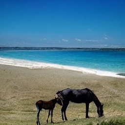
input + mask	“beach”	“a beach”	“a beach!”	“beaches”	“a day at the beach”

Figure 24. Prompt sensitivity: Our method is somewhat sensitive to the input prompt — the results may change slightly for small input prompt changes.

AAAA“stones”
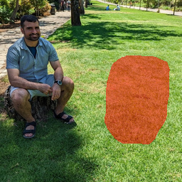
AAA“a blue ball”
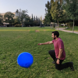
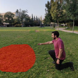
AAAA“a beach”
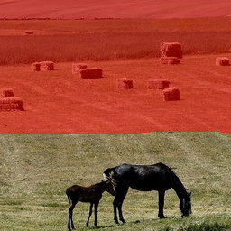
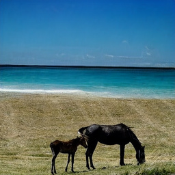
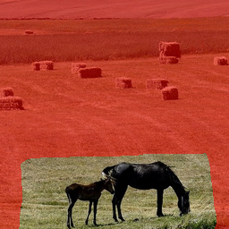
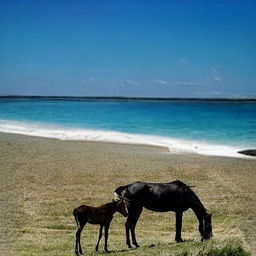
	input + mask	result	input + mask	result	input + mask	result

Figure 25. Mask sensitivity: Our method is somewhat sensitive to the input mask — the results may change for small input mask changes.

AAAA“stones”
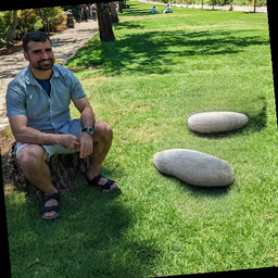
AAA“a blue ball”
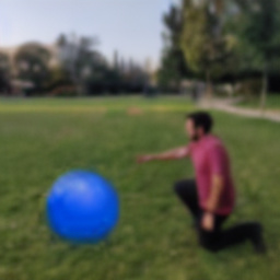
AAAA“a beach”
	input + mask	result	Rotated $5\degree$	result	Gaussian blur	result

Figure 26. Image sensitivity: Our method is somewhat sensitive to the input images — the results may change for small input image changes such as rotation and blur.

Appendix E Societal Impact

Lowering the barrier for content manipulations is a mixed blessing: on the one hand, it democratizes content creation, enhances creativity, and enables new applications. On the other hand, it can be used in a nefarious manner for generating fake news, harassing, bullying, and causing bad psychological and sociological effects (Fried et al., 2020). In addition, the LDM model was trained on LAION-400M dataset (Schuhmann et al., 2021) that consists of 400M text-image pairs that were collected from the internet. This dataset is non-curated, and as such may contain discomforting and disturbing content that may be repeated by the model. Moreover, it was shown (Nichol et al., 2021) that text-to-image generative models may inherit some of the biases in the training data, hence editing images guided by a text prompt may also suffer from this problem.

We strongly believe that despite these drawbacks, producing better content creation methods will produce a net positive to society.

References

(1)
Abdal et al. (2019)
Rameen Abdal, Yipeng Qin,
and Peter Wonka. 2019.
Image2stylegan: How to embed images into the
StyleGAN latent space?. In Proc. ICCV.
4432–4441.
Abdal et al. (2020)
Rameen Abdal, Yipeng Qin,
and Peter Wonka. 2020.
Image2stylegan++: How to edit the embedded
images?. In Proc. CVPR.
8296–8305.
Ashual et al. (2022)
Oron Ashual, Shelly
Sheynin, Adam Polyak, Uriel Singer,
Oran Gafni, Eliya Nachmani, and
Yaniv Taigman. 2022.
KNN-Diffusion: Image Generation via Large-Scale
Retrieval.
arXiv preprint arXiv:2204.02849
(2022).
Avrahami et al. (2022a)
Omri Avrahami, Thomas
Hayes, Oran Gafni, Sonal Gupta,
Yaniv Taigman, Devi Parikh,
Dani Lischinski, Ohad Fried, and
Xi Yin. 2022a.
SpaText: Spatio-Textual Representation for
Controllable Image Generation.
arXiv preprint arXiv:2211.14305
(2022).
Avrahami et al. (2022b)
Omri Avrahami, Dani
Lischinski, and Ohad Fried.
2022b.
Blended diffusion for text-driven editing of
natural images. In Proceedings of the IEEE/CVF
Conference on Computer Vision and Pattern Recognition.
18208–18218.
Bar-Tal et al. (2022)
Omer Bar-Tal, Dolev
Ofri-Amar, Rafail Fridman, Yoni Kasten,
and Tali Dekel. 2022.
Text2LIVE: Text-Driven Layered Image and Video
Editing.
arXiv preprint arXiv:2204.02491
(2022).
Bau et al. (2021)
David Bau, Alex Andonian,
Audrey Cui, YeonHwan Park,
Ali Jahanian, Aude Oliva, and
Antonio Torralba. 2021.
Paint by word.
arXiv preprint arXiv:2103.10951
(2021).
Bau et al. (2020)
David Bau, Hendrik
Strobelt, William Peebles, Jonas Wulff,
Bolei Zhou, Jun-Yan Zhu, and
Antonio Torralba. 2020.
Semantic photo manipulation with a generative image
prior.
arXiv preprint arXiv:2005.07727
(2020).
Bond-Taylor et al. (2021)
Sam Bond-Taylor, Peter
Hessey, Hiroshi Sasaki, Toby P Breckon,
and Chris G Willcocks. 2021.
Unleashing Transformers: Parallel Token Prediction
with Discrete Absorbing Diffusion for Fast High-Resolution Image Generation
from Vector-Quantized Codes.
arXiv preprint arXiv:2111.12701
(2021).
Bradski and Kaehler (2000)
Gary Bradski and Adrian
Kaehler. 2000.
OpenCV.
Dr. Dobb’s journal of software tools
3 (2000), 2.
Brock et al. (2018)
Andrew Brock, Jeff
Donahue, and Karen Simonyan.
2018.
Large scale GAN training for high fidelity
natural image synthesis.
arXiv preprint arXiv:1809.11096
(2018).
Choi et al. (2021)
Jooyoung Choi, Sungwon
Kim, Yonghyun Jeong, Youngjune Gwon,
and Sungroh Yoon. 2021.
ILVR: Conditioning Method for Denoising Diffusion
Probabilistic Models. In 2021 IEEE/CVF
International Conference on Computer Vision (ICCV). IEEE,
14347–14356.
Crowson et al. (2022)
Katherine Crowson, Stella
Biderman, Daniel Kornis, Dashiell
Stander, Eric Hallahan, Louis
Castricato, and Edward Raff.
2022.
VQGAN-CLIP: Open Domain Image Generation and
Editing with Natural Language Guidance.
arXiv preprint arXiv:2204.08583
(2022).
Deng et al. (2009)
Jia Deng, Wei Dong,
Richard Socher, Li-Jia Li,
Kai Li, and Li Fei-Fei.
2009.
ImageNet: A large-scale hierarchical image
database. In Proc. CVPR. Ieee,
248–255.
Dhariwal and Nichol (2021)
Prafulla Dhariwal and
Alexander Nichol. 2021.
Diffusion models beat GANs on image synthesis.
Advances in Neural Information Processing
Systems 34 (2021).
Ding et al. (2021)
Ming Ding, Zhuoyi Yang,
Wenyi Hong, Wendi Zheng,
Chang Zhou, Da Yin,
Junyang Lin, Xu Zou,
Zhou Shao, Hongxia Yang, et al.
2021.
Cogview: Mastering text-to-image generation via
transformers.
Advances in Neural Information Processing
Systems 34 (2021),
19822–19835.
Dosovitskiy et al. (2020)
Alexey Dosovitskiy, Lucas
Beyer, Alexander Kolesnikov, Dirk
Weissenborn, Xiaohua Zhai, Thomas
Unterthiner, Mostafa Dehghani, Matthias
Minderer, Georg Heigold, Sylvain Gelly,
et al. 2020.
An Image is Worth 16x16 Words: Transformers for
Image Recognition at Scale. In International
Conference on Learning Representations.
Esser et al. (2021b)
Patrick Esser, Robin
Rombach, Andreas Blattmann, and Bjorn
Ommer. 2021b.
ImageBART: Bidirectional context with multinomial
diffusion for autoregressive image synthesis.
Advances in Neural Information Processing
Systems 34 (2021).
Esser et al. (2021a)
Patrick Esser, Robin
Rombach, and Bjorn Ommer.
2021a.
Taming transformers for high-resolution image
synthesis. In Proc. CVPR.
12873–12883.
Fried et al. (2020)
Ohad Fried, Jennifer
Jacobs, Adam Finkelstein, and Maneesh
Agrawala. 2020.
Editing Self-Image.
Commun. ACM 63,
3, 70–79.
https://doi.org/10.1145/3326601
Gafni et al. (2022)
Oran Gafni, Adam Polyak,
Oron Ashual, Shelly Sheynin,
Devi Parikh, and Yaniv Taigman.
2022.
Make-a-scene: Scene-based text-to-image generation
with human priors.
(2022), 89–106.
Gal et al. (2022)
Rinon Gal, Or Patashnik,
Haggai Maron, Amit H Bermano,
Gal Chechik, and Daniel Cohen-Or.
2022.
StyleGAN-NADA: CLIP-guided domain adaptation of
image generators.
ACM Transactions on Graphics (TOG)
41, 4 (2022),
1–13.
Goodfellow et al. (2014)
Ian Goodfellow, Jean
Pouget-Abadie, Mehdi Mirza, Bing Xu,
David Warde-Farley, Sherjil Ozair,
Aaron Courville, and Yoshua Bengio.
2014.
Generative Adversarial Nets. In
Advances in Neural Information Processing
Systems. 2672–2680.
Gu et al. (2021)
Shuyang Gu, Dong Chen,
Jianmin Bao, Fang Wen,
Bo Zhang, Dongdong Chen,
Lu Yuan, and Baining Guo.
2021.
Vector quantized diffusion model for text-to-image
synthesis.
arXiv preprint arXiv:2111.14822
(2021).
Hertz et al. (2022)
Amir Hertz, Ron Mokady,
Jay Tenenbaum, Kfir Aberman,
Yael Pritch, and Daniel Cohen-Or.
2022.
Prompt-to-prompt image editing with cross attention
control.
arXiv preprint arXiv:2208.01626
(2022).
Ho et al. (2020)
Jonathan Ho, Ajay Jain,
and Pieter Abbeel. 2020.
Denoising Diffusion Probabilistic Models. In
Proc. NeurIPS.
Hu et al. (2021)
Minghui Hu, Yujie Wang,
Tat-Jen Cham, Jianfei Yang, and
PN Suganthan. 2021.
Global Context with Discrete Diffusion in Vector
Quantised Modelling for Image Generation.
arXiv preprint arXiv:2112.01799
(2021).
Karras et al. (2019)
Tero Karras, Samuli
Laine, and Timo Aila. 2019.
A style-based generator architecture for generative
adversarial networks. In Proceedings of the
IEEE/CVF Conference on Computer Vision and Pattern Recognition.
4401–4410.
Karras et al. (2020)
Tero Karras, Samuli
Laine, Miika Aittala, Janne Hellsten,
Jaakko Lehtinen, and Timo Aila.
2020.
Analyzing and improving the image quality of
StyleGAN. In Proceedings of the IEEE/CVF
Conference on Computer Vision and Pattern Recognition.
8110–8119.
Kingma and Ba (2014)
Diederik P Kingma and
Jimmy Ba. 2014.
Adam: A method for stochastic optimization.
arXiv preprint arXiv:1412.6980
(2014).
Kingma and Welling (2013)
Diederik P Kingma and
Max Welling. 2013.
Auto-encoding variational Bayes.
arXiv preprint arXiv:1312.6114
(2013).
Liu et al. (2021)
Xihui Liu, Dong Huk Park,
Samaneh Azadi, Gong Zhang,
Arman Chopikyan, Yuxiao Hu,
Humphrey Shi, Anna Rohrbach, and
Trevor Darrell. 2021.
More Control for Free! Image Synthesis with
Semantic Diffusion Guidance.
arXiv preprint arXiv:2112.05744
(2021).
Lugmayr et al. (2022)
Andreas Lugmayr, Martin
Danelljan, Andres Romero, Fisher Yu,
Radu Timofte, and Luc Van Gool.
2022.
Repaint: Inpainting using denoising diffusion
probabilistic models. In Proceedings of the
IEEE/CVF Conference on Computer Vision and Pattern Recognition.
11461–11471.
Mansimov et al. (2016)
Elman Mansimov, Emilio
Parisotto, Jimmy Ba, and Ruslan
Salakhutdinov. 2016.
Generating Images from Captions with Attention.
CoRR abs/1511.02793
(2016).
Meng et al. (2021)
Chenlin Meng, Yutong He,
Yang Song, Jiaming Song,
Jiajun Wu, Jun-Yan Zhu, and
Stefano Ermon. 2021.
Sdedit: Guided image synthesis and editing with
stochastic differential equations. In
International Conference on Learning
Representations.
Nichol et al. (2021)
Alex Nichol, Prafulla
Dhariwal, Aditya Ramesh, Pranav Shyam,
Pamela Mishkin, Bob McGrew,
Ilya Sutskever, and Mark Chen.
2021.
GLIDE: Towards photorealistic image generation
and editing with text-guided diffusion models.
arXiv preprint arXiv:2112.10741
(2021).
Nichol and Dhariwal (2021)
Alexander Quinn Nichol and
Prafulla Dhariwal. 2021.
Improved denoising diffusion probabilistic models.
In Proc. ICML. 8162–8171.
Paiss et al. (2022)
Roni Paiss, Hila Chefer,
and Lior Wolf. 2022.
No Token Left Behind: Explainability-Aided Image
Classification and Generation.
arXiv preprint arXiv:2204.04908
(2022).
Pan et al. (2021)
Xingang Pan, Xiaohang
Zhan, Bo Dai, Dahua Lin,
Chen Change Loy, and Ping Luo.
2021.
Exploiting deep generative prior for versatile
image restoration and manipulation.
IEEE Transactions on Pattern Analysis and
Machine Intelligence (2021).
Paszke et al. (2019)
Adam Paszke, Sam Gross,
Francisco Massa, Adam Lerer,
James Bradbury, Gregory Chanan,
Trevor Killeen, Zeming Lin,
Natalia Gimelshein, Luca Antiga,
et al. 2019.
Pytorch: An imperative style, high-performance deep
learning library.
Advances in neural information processing
systems 32 (2019),
8026–8037.
Patashnik et al. (2021)
Or Patashnik, Zongze Wu,
Eli Shechtman, Daniel Cohen-Or, and
Dani Lischinski. 2021.
StyleCLIP: Text-driven manipulation of StyleGAN
imagery. In Proceedings of the IEEE/CVF
International Conference on Computer Vision. 2085–2094.
Pérez et al. (2003)
Patrick Pérez, Michel
Gangnet, and Andrew Blake.
2003.
Poisson image editing.
In Proc. ACM SIGGRAPH 2003.
313–318.
Radford et al. (2021)
Alec Radford, Jong Wook
Kim, Chris Hallacy, Aditya Ramesh,
Gabriel Goh, Sandhini Agarwal,
Girish Sastry, Amanda Askell,
Pamela Mishkin, Jack Clark,
et al. 2021.
Learning transferable visual models from natural
language supervision.
arXiv preprint arXiv:2103.00020
(2021).
Ramesh et al. (2022)
Aditya Ramesh, Prafulla
Dhariwal, Alex Nichol, Casey Chu, and
Mark Chen. 2022.
Hierarchical text-conditional image generation with
CLIP latents.
arXiv preprint arXiv:2204.06125
(2022).
Ramesh et al. (2021)
Aditya Ramesh, Mikhail
Pavlov, Gabriel Goh, Scott Gray,
Chelsea Voss, Alec Radford,
Mark Chen, and Ilya Sutskever.
2021.
Zero-shot text-to-image generation.
arXiv preprint arXiv:2102.12092
(2021).
Razavi et al. (2019)
Ali Razavi, Aaron Van den
Oord, and Oriol Vinyals.
2019.
Generating diverse high-fidelity images with
VQ-VAE-2.
Advances in neural information processing
systems 32 (2019).
Reed et al. (2016)
Scott Reed, Zeynep Akata,
Xinchen Yan, Lajanugen Logeswaran,
Bernt Schiele, and Honglak Lee.
2016.
Generative adversarial text to image synthesis. In
Proc. ICLR. 1060–1069.
Roich et al. (2021)
Daniel Roich, Ron Mokady,
Amit H Bermano, and Daniel Cohen-Or.
2021.
Pivotal tuning for latent-based editing of real
images.
arXiv preprint arXiv:2106.05744
(2021).
Rombach et al. (2022)
Robin Rombach, Andreas
Blattmann, Dominik Lorenz, Patrick
Esser, and Björn Ommer.
2022.
High-resolution image synthesis with latent
diffusion models.
(2022), 10684–10695.
Saharia et al. (2022a)
Chitwan Saharia, William
Chan, Huiwen Chang, Chris Lee,
Jonathan Ho, Tim Salimans,
David Fleet, and Mohammad Norouzi.
2022a.
Palette: Image-to-image diffusion models. In
ACM SIGGRAPH 2022 Conference Proceedings.
1–10.
Saharia et al. (2022b)
Chitwan Saharia, William
Chan, Saurabh Saxena, Lala Li,
Jay Whang, Emily Denton,
Seyed Kamyar Seyed Ghasemipour,
Burcu Karagol Ayan, S Sara Mahdavi,
Rapha Gontijo Lopes, et al.
2022b.
Photorealistic Text-to-Image Diffusion Models with
Deep Language Understanding.
arXiv preprint arXiv:2205.11487
(2022).
Schuhmann et al. (2021)
Christoph Schuhmann,
Richard Vencu, Romain Beaumont,
Robert Kaczmarczyk, Clayton Mullis,
Aarush Katta, Theo Coombes,
Jenia Jitsev, and Aran Komatsuzaki.
2021.
Laion-400m: Open dataset of clip-filtered 400
million image-text pairs.
arXiv preprint arXiv:2111.02114
(2021).
Sohl-Dickstein et al. (2015)
Jascha Sohl-Dickstein,
Eric Weiss, Niru Maheswaranathan, and
Surya Ganguli. 2015.
Deep unsupervised learning using nonequilibrium
thermodynamics. In Proc. ICML.
2256–2265.
Song et al. (2020)
Jiaming Song, Chenlin
Meng, and Stefano Ermon.
2020.
Denoising Diffusion Implicit Models. In
International Conference on Learning
Representations.
Tan and Le (2019)
Mingxing Tan and Quoc
Le. 2019.
Efficientnet: Rethinking model scaling for
convolutional neural networks. In International
conference on machine learning. PMLR, 6105–6114.
Tzaban et al. (2022)
Rotem Tzaban, Ron Mokady,
Rinon Gal, Amit H Bermano, and
Daniel Cohen-Or. 2022.
Stitch it in Time: GAN-Based Facial Editing of Real
Videos.
arXiv preprint arXiv:2201.08361
(2022).
Vahdat et al. (2021)
Arash Vahdat, Karsten
Kreis, and Jan Kautz. 2021.
Score-based generative modeling in latent space.
Advances in Neural Information Processing
Systems 34 (2021),
11287–11302.
Van Den Oord et al. (2017)
Aaron Van Den Oord, Oriol
Vinyals, et al. 2017.
Neural discrete representation learning.
Advances in neural information processing
systems 30 (2017).
van den Oord et al. (2017)
Aäron van den Oord,
Oriol Vinyals, and Koray Kavukcuoglu.
2017.
Neural Discrete Representation Learning. In
NIPS.
Vaswani et al. (2017)
Ashish Vaswani, Noam
Shazeer, Niki Parmar, Jakob Uszkoreit,
Llion Jones, Aidan N Gomez,
Łukasz Kaiser, and Illia
Polosukhin. 2017.
Attention is all you need. In
Advances in neural information processing
systems. 5998–6008.
Wang et al. (2022)
Zihao Wang, Wei Liu,
Qian He, Xinglong Wu, and
Zili Yi. 2022.
CLIP-GEN: Language-Free Training of a
Text-to-Image Generator with CLIP.
arXiv preprint arXiv:2203.00386
(2022).
Xia et al. (2021)
Weihao Xia, Yulun Zhang,
Yujiu Yang, Jing-Hao Xue,
Bolei Zhou, and Ming-Hsuan Yang.
2021.
GAN inversion: A survey.
arXiv preprint arXiv:2101.05278
(2021).
Xu et al. (2018)
Tao Xu, Pengchuan Zhang,
Qiuyuan Huang, Han Zhang,
Zhe Gan, Xiaolei Huang, and
Xiaodong He. 2018.
AttnGAN: Fine-grained text to image generation
with attentional generative adversarial networks. In
Proceedings of the IEEE conference on computer
vision and pattern recognition. 1316–1324.
Yu et al. (2022)
Jiahui Yu, Yuanzhong Xu,
Jing Yu Koh, Thang Luong,
Gunjan Baid, Zirui Wang,
Vijay Vasudevan, Alexander Ku,
Yinfei Yang, Burcu Karagol Ayan,
et al. 2022.
Scaling Autoregressive Models for Content-Rich
Text-to-Image Generation.
arXiv preprint arXiv:2206.10789
(2022).
Zhang et al. (2017)
Han Zhang, Tao Xu,
Hongsheng Li, Shaoting Zhang,
Xiaogang Wang, Xiaolei Huang, and
Dimitris N Metaxas. 2017.
StackGAN: Text to photo-realistic image synthesis
with stacked generative adversarial networks. In
Proc. ICCV. 5907–5915.
Zhang et al. (2018b)
Han Zhang, Tao Xu,
Hongsheng Li, Shaoting Zhang,
Xiaogang Wang, Xiaolei Huang, and
Dimitris N Metaxas. 2018b.
StackGAN++: Realistic image synthesis with
stacked generative adversarial networks.
IEEE transactions on pattern analysis and
machine intelligence 41, 8
(2018), 1947–1962.
Zhang et al. (2018a)
Richard Zhang, Phillip
Isola, Alexei A Efros, Eli Shechtman,
and Oliver Wang. 2018a.
The unreasonable effectiveness of deep features as
a perceptual metric. In Proceedings of the IEEE
conference on computer vision and pattern recognition.
586–595.
Zhou et al. (2021)
Yufan Zhou, Ruiyi Zhang,
Changyou Chen, Chunyuan Li,
Chris Tensmeyer, Tong Yu,
Jiuxiang Gu, Jinhui Xu, and
Tong Sun. 2021.
LAFITE: Towards Language-Free Training for
Text-to-Image Generation.
arXiv preprint arXiv:2111.13792
(2021).
Zhu et al. (2020)
Jiapeng Zhu, Yujun Shen,
Deli Zhao, and Bolei Zhou.
2020.
In-domain GAN inversion for real image editing.
In Proc. ECCV. Springer,
592–608.