CORE: Consistent Representation Learning for Face Forgery Detection

Abstract

Face manipulation techniques develop rapidly and arouse widespread public concerns. Despite that vanilla convolutional neural networks achieve acceptable performance, they suffer from the overfitting issue. To relieve this issue, there is a trend to introduce some erasing-based augmentations. We find that these methods indeed attempt to implicitly induce more consistent representations for different augmentations via assigning the same label for different augmented images. However, due to the lack of explicit regularization, the consistency between different representations is less satisfactory. Therefore, we constrain the consistency of different representations explicitly and propose a simple yet effective framework, COnsistent REpresentation Learning (CORE). Specifically, we first capture the different representations with different augmentations, then regularize the cosine distance of the representations to enhance the consistency. Extensive experiments (in-dataset and cross-dataset) demonstrate that CORE performs favorably against state-of-the-art face forgery detection methods. Our code is available at https://github.com/niyunsheng/CORE.

1 Introduction

With the rapid development of face manipulation techniques (e.g. autoencoder-based [29] and GAN-based [24, 33, 22]), synthetic faces become extremely hard for humans to distinguish from real faces. This causes a considerable risk to the trust and security of society. Thus, it is important to develop effective methods for face forgery detection.

Since a vanilla convolutional neural network (CNN) has achieved acceptable performance, it suffers from the overfitting issue [26, 43, 38, 34, 30, 6, 14] due to oversampling the real faces to generate the fake samples. To relieve this issue, recent works [43, 14] introduce some effective erasing-based data augmentations. They erase different regions of a sample to capture more general forgery representation. In fact, through observing their class activation mapping (CAM), we find that the erasing-based methods tend to implicitly induce more consistent representations for the sample of different data augmentations. Nevertheless, due to the lack of explicit regularization, the consistency between different representations is less satisfactory. Therefore, we explicitly constrain the representation distances between different data augmentations to capture more intrinsic forgery evidence.

Figure 1: An illustration of the CORE framework compared to traditional methods. The right column shows the Class Activation Mapping (CAM) of input of erasing different parts. The CAM is more consistent in our method. Aug. refers to data augmentations.

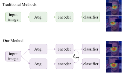
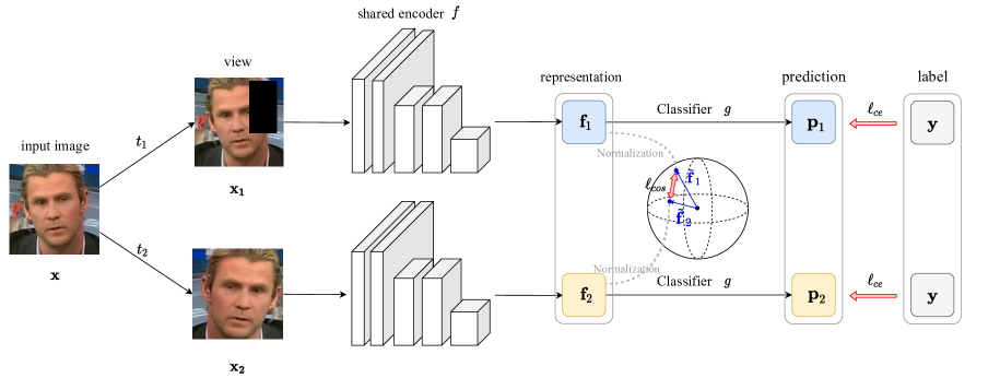
In this paper, we propose a simple yet effective framework, Consistent Representation Learning (CORE), to explicitly learn consistent representations for face forgery detection. As shown in Fig. 1, the proposed framework adopts paired random augmentations to transform the input to different views. A shared Encoder extracts the corresponding feature representations for the transformed inputs. We explicitly constrain the consistency of the different representations via a Consistency Loss. Finally, a Classifier Network assigns the supervised label for each representation.

Compared with the traditional methods, the proposed framework has two merits: (1) The representations of different augmentations are regularized explicitly, which enables the model to attend to more intrinsic forgery evidence. (2) Our framework does not modify the model structure and can be flexibly integrated with almost any other method.

The main contributions of our work are as follows:

1. We propose a simple yet effective framework, Consistent Representation Learning (CORE). This framework captures different representations of the same sample via different augmentations, and constrains them consistent explicitly with the Consistency Loss.

2. The proposed framework enables a vanilla CNN model to obtain state-of-the-art performance on FF++ [36](RAW, HQ), Celeb-DF [29], and DFFD [13] benchmarks for in-dataset evaluation, on DFD [17] for cross-dataset evaluation.

2 Related Work

Face forgery detection. Most recent works formulate face forgery detection as a binary classification problem. FaceForensics++ (FF++) [36] proposes a benchmark and provide a baseline with a vanilla Xception [9] network. Patch [4] regards the input image as some patches and uses a shallow network as the backbone. Face X-ray [26] aims to localize the blending boundary in a self-supervised mechanism. Multi-attention [50] proposes a novel multi-attentional network architecture. Two-branch RN [32] learns representations combining the color domain and the frequency domain. F3-Net [34] and RFAM [6] mine clues in the frequency domain, and achieve impressive performance in low-quality videos. LSC [51] hypothesizes that images’ distinct source features can be preserved and extracted after going through deepfake generation processes. Thus the inconsistency of source features can be used to detect deepfakes generations. Our proposed method CORE tries to learn consistent representation for face forgery detection that is invariant to data augmentations.

Figure 2: An illustration of the architecture of Consistent Representation Learning. We first adopt two different data augmentations to the input image $\mathbf{x}$ and get two views $\mathbf{x_{1}}$ and $\mathbf{x_{2}}$. Then we feed the two views into a shared encoder $f$ and get two representations $\mathbf{f_{1}}$ and $\mathbf{f_{2}}$. We feed the two representations into a classifier $g$ and use a cross-entropy loss to train the network, as well as adopt a cosine similarity loss $\ell_{cos}$ to penalize the distance between $\mathbf{f_{1}}$ and $\mathbf{f_{2}}$.

Data augmentation. Data augmentations are proven to be useful in computer vision problems. Random Erasing [53] randomly erases a rectangle area of the input. Adversarial Erasing [45] is initially used in the weakly supervised semantic segmentation, which erases the activate areas produced by Class Activation Mapping (CAM) [54]. Some works study the data augmentations in face forgery detection [3, 5, 43, 14]. RFM [43] traces the facial region which is sensitive to the network and erases the top-N areas. Face-Cutout [14] uses the facial landmarks and randomly cuts out the face part (eg. mouth, eye, etc.) Data augmentations help to learn representations invariant to certain transformations. We explicitly force the model to learn certain invariance by a consistency loss.

Consistency learning. Consistency learning, enforcing the predictions or features of different views for the same unlabeled instance to be similar, has been widely applied in semi-supervised learning, such as $\Pi$ Model [25], Temporal Ensemble [25], and Mean Teacher [40]. We show that learning consistent representations is also helpful for face forgery detection under a fully-supervised setting.

Contrastive learning. Contrastive learning achieves great success in unsupervised visual representation learning. MoCo [20], SimCLR [7], InstDisc [46] build instance-level contrastive learning framework. PixPro [47], DenseCL [44] build pixel-wise contrastive learning framework. There are some recent works [11, 19, 48] introduce contrastive learning into face forgery detection and get a considerable generalization performance. These methods adopt popular instance discrimination based or pixel wise contrastive learning framework for face forgery detection. We do not apply instance-level or pixel-level contrastive learning. Instead, we only use consistency regularization to learn representation that attend to extract more intrinsic forgery evidence.

3 Proposed Method

3.1 Preliminaries

Face forgery detection is often formulated as a binary classification problem. The face forgery detection pipeline follows the standard image classification pipeline: data pre-processing (including data augmentation), feature extraction, and prediction through a classifier. As shown in Fig. 2, we generate two views of the same image by applying random data augmentation twice, and penalize the distance between the representations of the two views.

3.2 Consistent Representation Learning Framework

Given an input batch of $N$ images, we first apply random data augmentations twice to obtain $2N$ images ($N$ pairs). Then we put the augmented images to an encoder and get $2N$ representation vectors. The representation vectors are fed into a classifier to obtain classification scores. Moreover, we apply a consistency loss on the representation vectors from a pair of images for explicitly learning augmentation invariance.

As illustrated in Fig. 2, our framework is composed of three components: data augmentation, encoder network, and classifier network.

Data augmentation. Given a set of transformations $\mathcal{T}$ and an input image $\mathbf{x}$, two transformations $t_{1},t_{2}$ are randomly sampled from $\mathcal{T}$ to serve as data augmentations. Two views of the image are produced through the two augmentations: $\mathbf{x}_{1}=t_{1}(\mathbf{x})$, $\mathbf{x}_{2}=t_{2}(\mathbf{x})$. The data augmentations should not alter the intrinsic property of its genuineness. See Sec. 4.2 for more details about data augmentations.

Encoder network. We use a Xception[9] network as our encoder network $f$. The encoder network maps the two views of input image $\mathbf{x}_{1},\mathbf{x}_{2}$ into two $d-$dimensional representation vectors $\mathbf{f}_{1}=f(\mathbf{x}_{1}),\mathbf{f}_{2}=f(\mathbf{x}_{2})$. The two representation vectors are fed into a classifier network for classification, as well as for consistency loss computation.

Classifier network. The classifier network (donate as $g$) contains a linear layer and a softmax normalization layer, mapping a representation vector $\mathbf{f}$ into a scalar probability $p$ (we adopt the second dimension of the output after softmax layer as final probability), $p=g(\mathbf{f})$. The output probability is used for fake face classification.

3.3 Loss Functions

Consistency loss. Given this framework, then we introduce the consistency loss. The consistency loss is used to penalize the distances of the representation vectors that are extracted from different views of the same original image.

We adopt cosine similarity loss ($\ell_{cos}$) to penalize the distance between the two representation vectors, as follows:

$$\ell_{cos}\left(\mathbf{f}^{(n)}_{1},\mathbf{f}^{(n)}_{2}\right)=\left(1-\tilde{\mathbf{f}}^{(n)}_{1}\cdot\tilde{\mathbf{f}}^{(n)}_{2}\right)^{2}$$ (1)

where $\tilde{\mathbf{f}}=\frac{\mathbf{f}}{\|\mathbf{f}\|_{2}}$ denotes the normalized vector of the representation vector $\mathbf{f}$. As illustrated in Fig. 2, feature used for the similarity computation is normalized by a L$2$ normalization layer firstly. For $N$ pairs of input images, the consistency loss can be written as

$$\mathcal{L}_{c}=\sum_{n=1}^{N}\ell_{cos}\left(\mathbf{f}^{(n)}_{1},\mathbf{f}^{(n)}_{2}\right)=\sum_{n=1}^{N}\left(1-\tilde{\mathbf{f}}^{(n)}_{1}\cdot\tilde{\mathbf{f}}^{(n)}_{2}\right)^{2}$$ (2)

Cosine similarity loss only pulls the angle of the vectors to be similar, ignoring the norm of the vectors. The reason we choose to use cosine similarity is that we do not force the representations of different views to be exactly the same. As shown in Fig. 2, the RE augmentation can cut out a region in the face, which makes the information in the two views not identical. In this case, forcing the representation to be the same might harm to the learned representations. Thus, we use cosine loss instead of L1 or L2 loss that also forces the norm of two vectors to be the same. Empirical analysis on different consistency losses is given in Sec. 4.3.

Classification loss. We use standard cross-entropy loss as classification loss:

$$\ell_{ce}(p)=y\log{p}+(1-y)\log(1-p)$$ (3)

where $y$ is the ground-truth label. For $N$ pairs of input images, the classification loss can be written as

$$\mathcal{L}_{ce}=\sum_{n=1}^{N}\left(\ell_{ce}\left(p^{(n)}_{1}\right)+\ell_{ce}\left(p^{(n)}_{2}\right)\right)$$ (4)

Overall loss. We combine the consistency loss with the cross-entropy loss to form the overall loss in our framework:

$$\mathcal{L}=\mathcal{L}_{ce}+\alpha\mathcal{L}_{c}$$ (5)

Here $\alpha$ is a balance weight for the two losses.

4 Experiments

4.1 Dataset

We conduct extensive experiments on five well-known datasets: FaceForensics++ (FF++) [36], Celeb-DF [29], DFFD [13], DFDC Preview (DFDC-P) [16] and deepfakeDetection (DFD) [17]. FF++ is a widely used face forgery dataset. There are a total of $1000$ real videos ($720$ videos for training, $140$ videos for validation, $140$ videos for testing) and $4,000$ manipulated videos generated with four forgery methods. Celeb-DF contains $5,939$ high-quality manipulated videos and $590$ real video clips collected from YouTube. Using improved synthesis process forgery faces in Celeb-DF are more realistic with fewer traces of forgery visible to human eyes. DFFD is more diverse in manipulated types compared to other datasets. There are $58,703$ real and $240,336$ fake still images along with $1,000$ real and $3,000$ fake video clips. Especially, the Deepfacelab subset in DFFD is not available, so we evaluate the metrics following [43] without the Deepfacelab subset. DFDC-P are mainly low-quality videos and diverse in several axes (gender, skin-tone, age, etc.). There are $4,119$ manipulated videos and $1,131$ real videos. DFD is released as a complement to the FF++ dataset, which contains $363$ real videos and $3,068$ fake videos.

4.2 Implementation Details

Data pre-processing. For each video in Celeb-DF, we extract $3$ frames per second. For each video in FF++, we sample $270$ frames per video following [36]. For videos in DFD and DFDC-P, we random select $50$ frames per video. We crop the faces with bounding boxes (detected boxes enlarged $1.3\times$) which is provided by MTCNN [49]. Some errors that crop real faces in manipulated videos occur whether select the biggest or highest detection probability face by MTCNN, especially when there are two characters in a video. We solved the problem by using the provided video mask in FF++.

Data augmentation. For data augmentation, we use two basic transformations: Random Erasing (RE) [53], and Random Resized Crop (RandCrop) and two complex augmentation strategies. For RE transformation, we use scale factor $(0.02,0.2)$ and aspect ratio $(0.5,2)$. For RandCrop transformation, scale factor $(1/1.3,1)$ and aspect ratio $(0.9,1.1)$ are adopted. For each input image, there is $1/3$ probability that the image is not augmented, $1/3$ probability that RE is applied, $1/3$ probability that RandCrop is applied. We denote this data augmentation strategy as RaAug. Additionally, we use another complex data augmentation contains quality compression, Gauss noise, Gauss blur, random shift, random scale, see [37] for more details. We denote this data augmentation strategy as DFDC_selim.

Training. All models are trained using Adam [23] with a constant learning rate of $0.0002$. We set the input size $299\times 299$ and mini-batch $32$. All of our models use Xception [9] as the backbone. All the models are trained within $30$ epochs and with early stopping if no gains are observed in consecutive $5$ epochs. We adopt a weight of $(4,1)$ for cross-entropy loss in all experiments to reduce the implicate of less real data. ImageNet [15] pretrained weights are used as parameter initialization.

Evaluation. We report Area Under Curve (AUC) as the main metric and accuracy (Acc.) as the secondary metric. For in-dataset experiments, we adopt True Detect Rate (TDR) at False Detect Rate (FDR) of $0.01\%$ (denoted as TDR_0.01%) and $0.1\%$ (denoted as TDR_0.1%) as a supplementary following [13].

Table 1: In-dataset comparison between consistent representation learning to Xception, and Xception+ (Xception trained with Random Erasing data augmentation). Our approach performs better than Xception+, which verifies the effectiveness of proposed consistent representation learning.

Method	AUC	TDR0.1%	TDR0.01%
Xception	$99.923$	$92.869$	$83.764$
Xception+	$99.930$	$91.806$	$86.318$
Ours	$\mathbf{99.943}$	$\mathbf{94.142}$	$\mathbf{88.388}$

Table 2: In-dataset ablation study on different penalties for consistency loss. Cosine penalty performs the best.

Penalty	AUC	TDR0.1%	TDR0.01%
$-$	$99.930$	$93.059$	$87.239$
L$1$	$99.938$	$93.295$	$84.653$
L$2$	$99.930$	$91.377$	$83.286$
Cos.	$\mathbf{99.943}$	$\mathbf{94.142}$	$\mathbf{88.388}$

Forgery Region

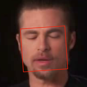
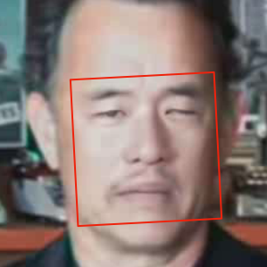
CAM

Figure 3: Visualizations of Class Activation Mapping (CAM) of CORE. The CAM highlights an area inside the forgery region.

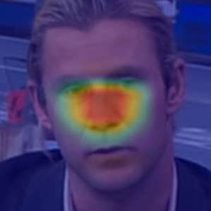
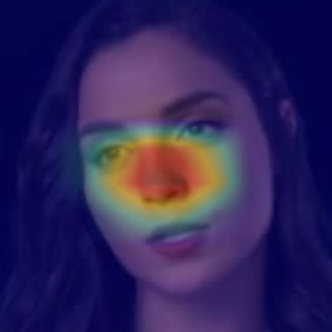
4.3 In-dataset Ablation Study

In this section, we validate the effectiveness of our proposed consistent representation learning approach and study two key components in our method: consistency loss and data augmentation. We uses Xception as backbone in all experiments. For in-dataset ablation study, we conduct experiments on Celeb-DF dataset. We use Random Erasing data augmentation and balance weight $\alpha=1$ as default.

Effectiveness of consistent representation learning. We compare our consistent representation learning approach with two baselines: Xception and Xception+. Xception refers to an Xception network trained without data augmentation. Xception+ refers to Xception trained with Random Erasing augmentation. Our approach adopts the same RE data augmentation as Xception+. As shown in Tab. 1, Xception+ performs better than Xception, and our approach performs best, outperforming Xception+ by $0.013$ AUC, $2.336$ TDR_0.1%, and $2.070$ TDR_0.01%.

Ablation study on consistency loss. We study three penalties for consistency loss: L1, L2, and cosine penalty. As shown in Tab. 2, model with L1 or L2 penalty performs on par or better than baseline for AUC, while worse for TDR_0.01%. Model with cosine penalty performs better than baseline on all AUC, TDR_0.1%, and TDR_0.01% metrics. We guess the reason for the unsatisfactory performance of L1 and L2 penalty might be that: forcing representations of two views to be identical is harmful to feature learning.

Table 3: In-dataset ablation study on balance weight $\alpha$. Model with $\alpha=2$ performs the best.

$\alpha$	$0$	$1$	$2$	$5$	$10$	$100$
AUC	$99.930$	$99.943$	$\mathbf{99.960}$	$99.943$	$99.948$	$99.915$

Table 4: In-dataset ablation study on data augmentation. Our approach performs consistently better than baseline on all augmentations. Ours with RaAug performs the best.

Data Aug.	Method	AUC	TDR0.1%	TDR0.01%
None	Baseline	$99.923$	$92.869$	$83.764$
RE	Baseline	$99.930$	$91.806$	$86.318$
	Ours	$99.960$	$\mathbf{95.670}$	$90.562$
RFM	Baseline	$99.926$	$91.768$	$84.419$
	Ours	$99.947$	$95.014$	$93.742$
RandCrop	Baseline	$99.929$	$89.432$	$84.504$
	Ours	$99.945$	$91.823$	$84.065$
RaAug	Baseline	$99.909$	$90.553$	$85.615$
	Ours	$\mathbf{99.971}$	$95.575$	$\mathbf{93.980}$
DFDC_selim	Baseline	$99.895$	$90.256$	$83.732$
	Ours	$99.941$	$93.970$	$88.737$

Ablation study on balance weight $\alpha$. We explore the balance weight setting for consistency loss in Tab. 3. In all cases except $\alpha=100$, consistent representation learning improves the performance of the model trained without consistency loss, and we find that model with $\alpha=2$ achieves the best performance.

Ablation study on data augmentation. We conduct experiments on different data augmentation strategies: RE [53], RFM [43], RandCrop, and proposed RaAug (see Sec. 4.2 for details). We use Xception models trained with the same data augmentation as baselines and balance weight $\alpha=2$. As shown in Tab. 4, our model consistently outperforms baseline under all data augmentations, by $+0.02$ to $+0.07$ AUC improvement and $+2.4$ to $+5.0$ TDR_0.1% improvement. Especially, RaAug performs overall the best among four data augmentation strategies, with $99.971$ AUC and $93.980$ TDR_0.01% score. We use RaAug as the default data augmentation strategy for our approach when compared with other methods for in-dataset evaluation.

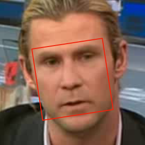
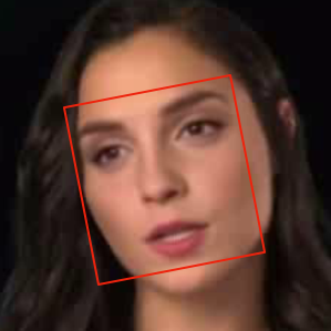
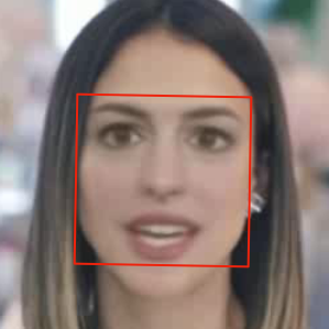
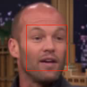
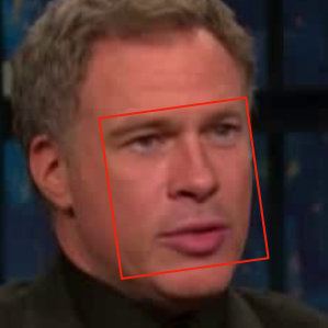
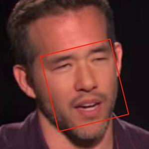
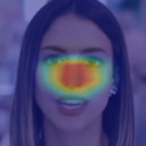
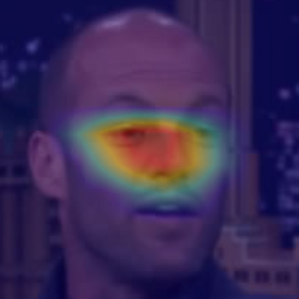
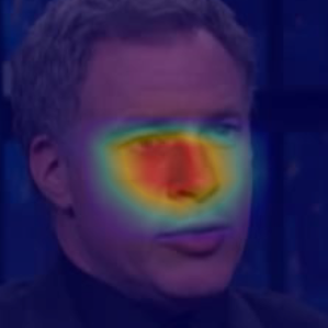
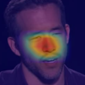
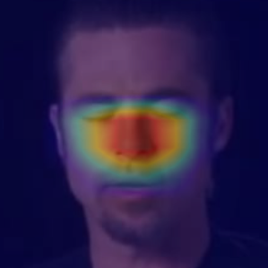
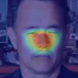
CAM visualizations. We visualize the Class Activation Mapping (CAM) of our approach in Fig. 3. The CAM highlights an area inside the forgery region.

4.4 Cross-dataset Ablation Study

In this section, we conduct the same experiments across datasets. We train our models on FF++ (HQ) dataset and evaluate on three datasets: DFD, DFDC-P and Celeb-DF. We use DFDC_selim data augmentation and balance weight $\alpha=1$ as default.

Table 5: Cross-dataset comparison between consistent representation learning to Xception, and Xception+ (Xception trained with DFDC_selim data augmentation). Avg refers to average of AUCs. Our proposed method outperforms than Xception+ under Avg. ^† Our reproduced result.

Method	DFD	DFDC-P	Celeb-DF	Avg
Xception [9]	${87.860}$	$64.724^{\dagger}$	$73.040$	$75.208$
Xception+	95.128	$70.725$	$70.010$	$78.621$
Ours	$94.090$	72.410	75.718	80.739

(a) Baseline on FF++(Test)
AUC = $98.00$.

(b) CORE on FF++(Test)
AUC = $99.04$.

Figure 4: An illustration of the feature distribution of baseline model (trained with DFDC_selim data augmentation) and CORE on the intra-domain dataset (FF++) via t-SNE.

Table 6: Cross-dataset ablation study on different penalties for consistency loss. Cosine penalty performs the best under the average AUC.

Penalty	DFD	DFDC-P	Celeb-DF	Avg
$-$	$95.128$	$70.725$	$70.010$	$78.621$
L$1$	95.621	$67.762$	$69.853$	$77.745$
L$2$	$95.131$	$67.334$	$75.374$	$76.976$
Cos.	$94.090$	72.410	75.718	80.739

Table 7: Cross-dataset ablation study on balance weight $\alpha$. Model with $\alpha=100$ performs the best under the average AUC.

$\alpha$	DFD	DFDC-P	Celeb-DF	Avg
$0$	$95.128$	$70.725$	$70.010$	$78.621$
$1$	$94.090$	$72.410$	$75.718$	$80.739$
$2$	96.137	$74.834$	${77.267}$	${82.746}$
$5$	$95.981$	$72.158$	$77.091$	$81.743$
$10$	$93.489$	76.264	$75.737$	$81.830$
$100$	$93.736$	$75.741$	79.448	82.975

Table 8: Cross-dataset ablation study on data augmentation. Our approach performs consistently better than baseline on all augmentations. Ours with DFDC_selim performs the best. ^† Our reproduced result.

Data Aug.	DFD	DFDC-P	Celeb-DF	Avg
None	${87.860}$	$64.724^{\dagger}$	$73.040$	$75.208$
RaAug	96.188	$67.186$	$66.983$	$76.786$
DFDC_selim	$93.736$	75.741	79.448	82.975

Effectiveness of consistent representation learning. In this section, Xception+ refers to Xception trained with DFDC_selim data augmentation. We select different data augmentation from the in-dataset experiments because different data augmentations have different effects on generalization performance. Ours adopts the same data augmentation as Xception+. As shown in Tab. 5, Xception+ outperforms than Xception. We used AUC as the default metric in cross-dataset ablation study experiments. Our proposed method outperforms Xception+ under the average AUC by $2.118\%$. In particular, our proposed method achieves a $5.708$ AUC gain under Celeb-DF dataset.

Ablation study on consistency loss. As shown in Tab. 6, different penalties show a similar effect as the in-dataset experiments. Cosine penalty performs better than L1 and L2 penalties under the average AUC. This proves that consistency representation learning also works across datasets.

Table 9: In-dataset SOTA comparisons on FF++ dataset. Our proposed approach performs the best under RAW and HQ quality settings. ^‡ we report the results provided in FF++ paper [36].

Method	Reference	RAW		HQ		LQ
		Acc.	AUC	Acc.	AUC	Acc.	AUC
Steg. Features [18]‡	IEEE TIFS 2012	$97.63$	$-$	$70.97$	$-$	$55.98$	$-$
C-Conv [2]‡	IH&MMSec 2016	$98.74$	$-$	$82.97$	$-$	$66.84$	$-$
LD-CNN [12]‡	IH&MMSec 2017	$98.57$	$-$	$78.45$	$-$	$58.69$	$-$
CP-CNN [35]‡	WIFS 2017	$97.03$	$-$	$79.08$	$-$	$61.18$	$-$
Xception [9]‡	CVPR 2017	$99.26$	$-$	$95.73$	$-$	$86.86$	$-$
MesoNet [1]‡	WIFS 2018	$95.23$	$-$	$83.10$	$-$	$70.47$	$-$
Two-branch RN [32]	ECCV 2020	$-$	$-$	$96.43$	$88.70$	$86.34$	$86.59$
F3-Net [34]	ECCV 2020	$99.95$	$99.80$	$97.52$	$98.10$	$90.43$	$93.30$
DeepfakeUCL [19]	IJCNN 2021	$-$	$-$	$-$	$93.00$	$-$	$-$
RFAM [6]	AAAI 2021	$99.87$	$99.92$	$97.59$	$99.46$	$\mathbf{91.47}$	$\mathbf{95.21}$
SPSL [30]	CVPR 2021	$-$	$-$	$91.50$	$95.32$	$81.57$	$82.82$
Multi-attention [50]	CVPR 2021	$-$	$-$	$97.60$	$99.29$	$88.69$	$90.40$
CORE		$\mathbf{99.97}$	$\mathbf{100.00}$	$\mathbf{97.61}$	$\mathbf{99.66}$	87.99	90.61

Table 10: In-dataset SOTA comparisons on CELEB-DF dataset. Our proposed approach performs the best. ^† we report the results provided in  [43].

Method	Acc.	AUC	TDR@$0.1\%$	TDR@$0.01\%$
Hu et al. [21]	$80.74$	$87.00$	$-$	$-$
FakeCatcher [10]	$91.50$	$-$	$-$	$-$
XcepTemporal [8]	$97.83$	$-$	$-$	$-$
Xception [9]†	$-$	$99.85$	$89.11$	$84.22$
RE [53]†	$-$	$99.84$	$84.05$	$76.63$
AE [45]†	$-$	$99.89$	$88.11$	$85.20$
Patch [4]†	$-$	$99.96$	$91.83$	$86.16$
RFM-X [43]†	$-$	$99.94$	$93.88$	$87.08$
RFM-Patch [43]†	$-$	$\mathbf{99.97}$	$93.44$	$89.58$
CORE	$\mathbf{99.17}$	$\mathbf{99.97}$	$\mathbf{95.58}$	$\mathbf{93.98}$

Table 11: In-dataset SOTA comparisons on DFFD dataset. Our proposed method performs the best. ^† we report the results provided in  [13].

Method	AUC	TDR0.1%	TDR0.01%
Xception [9]†	$99.61$	$85.26$	$77.42$
Reg-Xception [13]†	$99.64$	$90.78$	$83.83$
RFM-Xception [43]	$99.97$	$98.35$	$95.50$
CORE	$\mathbf{99.99}$	$\mathbf{99.23}$	$\mathbf{98.15}$

Table 12: In-dataset SOTA comparisons on DFDC-P dataset. Our proposed approach achieve similar performance to the SOTA method.

Method	Acc.	AUC
Tolosanaet al. [41]	$-$	$91.10$
S-MIL-T [27]	$-$	$85.11$
LSC [51]	$-$	94.38
CORE	$84.38$	$92.31$

Ablation study on balance weight $\alpha$. As in in-dataset experiments, we explore some different balance weight $\alpha$. As illustrated in Tab. 7, $\alpha=100$ performs better under the average AUC and most datasets. The best balance weight differs between the in-dataset and cross-dataset experiments. This shows that stronger consistency constraints work better in cross-domain experiments.

Ablation study on data augmentation. We also conduct experiments on different data augmentation strategies: proposed RaAug and DFDC_selim (see Sec. 4.2 for details) under $\alpha=100$. As shown in Tab. 8, data augmentation strategy plays an important role in CORE framework, which improves model generalization by a big gap. DFDC_selim achieves big gain in all three datasets. This shows that more complex data augmentation performs better in cross-domain experiments.

Table 13: Cross-dataset evaluation results on DFD, DFDC-P and Celeb-DF in terms of AUC. Our proposed method achieves highest AUC on DFD dataset and second highest AUC on DFDC-P and Celeb-DF dataset.

Method	Reference	Backbone	Train Set	DFD	DFDC-P	Celeb-DF
Xception [9]	CVPR 2017	Xception	FF++	$87.86$	$-$	$73.04$
DSP-FWA [28]	CVPRW 2019	ResNet-50	FF++	$-$	$-$	$69.30$
EfficientNet [39]	ICML 2019	EfficientNet-B4	FF++	$-$	$-$	$64.29$
Face X-ray [26]	CVPR 2020	HRNet	BI (private dataset)	$93.47$	$71.15$	$74.76$
Two-branch RN [32]	ECCV 2020	LSTM	FF++	$-$	$-$	$73.41$
F3-Net [34]	ECCV 2020	Xception	FF++	$-$	$-$	$76.88$
DeepfakeUCL [19]	IJCNN 2021	Xception	FF++	$-$	$-$	$56.80$
Local-relation [6]	AAAI 2021	Xception	FF++	$89.24$	76.53	$78.26$
HFF [31]	CVPR 2021	Xception (modified)	FF++	$91.90$	$-$	$79.4$
Multi-attention [50]	CVPR 2021	EfficientNet-B4	FF++	$-$	$-$	$67.44$
SPSL [30]	CVPR 2021	Xception	FF++	$-$	$-$	$76.88$
LSC [51]	ICCV 2021	ResNet-$34$	FF++ (real data)	$-$	$74.37$	$\mathbf{81.80}$
CORE		Xception	FF++	$\mathbf{93.74}$	$75.74$	$79.45$

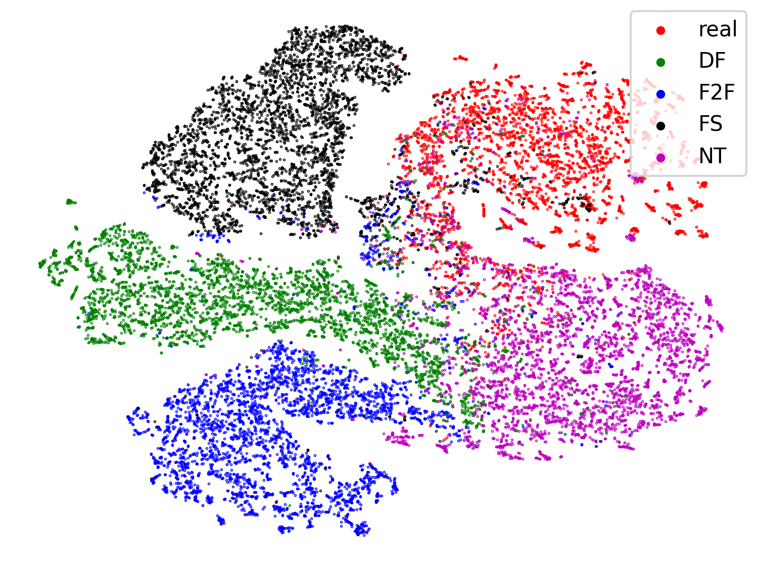
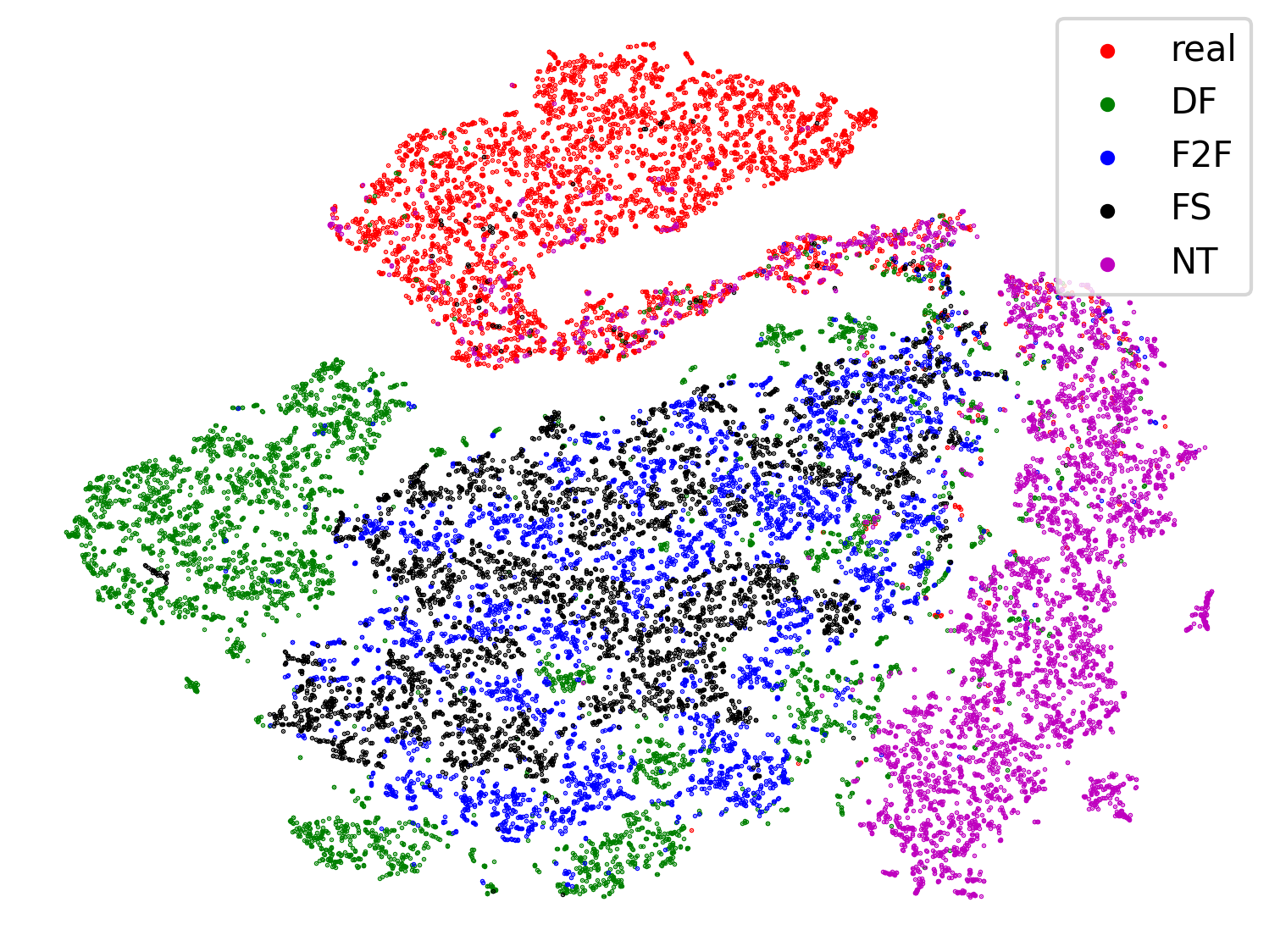
t-SNE visualizations. We visualize the feature distribution of the test part of FF++ dataset via t-SNE [42]. FTCN [52] observes that the CNN model can easily extract the unique artifacts of different manipulated methods, even if training with all manipulated data as one class. As illustrated in Fig. 4(a) and Fig. 4(b), the baseline model can separate four different forgery methods with a gap than CORE. CORE doesn’t distinguish the type of forgery algorithm to some degree. This indicates that CORE extracts the essential features for forgery detection instead of manipulated artifacts. Tab. 8 shows that CORE achieve $6.408$ AUC gains under Celeb-DF and $11.017$ AUC gains under DFDC-P dataset.

4.5 In-Dataset Comparison to Other Methods

In this section, we compare our method with previous forgery detection methods under four datasets: FF++, Celeb-DF, DFFD and DFDC-P.

Evaluation on FaceForensics++. The comparisons are shown in Tab. 9. Our approach outperforms all the other methods under RAW and HQ quality settings. Compared with Xception [36], which uses the same backbone network, our method performs better under all quality settings. Our method performs better than DeepfakeUCL [19], which adopts the contrastive learning method. For LQ setting, our method performs inferior to RFAM and F3-Net, similar to Multi-attention. RFAM and F3-Net encode features in the frequency domain, which has proven to be effective for LQ images. We do not adopt frequency-domain processing modules and this might lead to the superior performance of their approaches to ours.

Evaluation on Celeb-DF. As shown in Tab. 10, our method performs the best, achieving $91.17$ in ACC, $99.97$ in AUC, $95.58$ in TDR_0.1%, and $93.98$ in TDR_0.01%. Compared with the previous state-of-the-art method Patch, our approach improves TDR_0.1% and TDR_0.01% with a large margin.

Evaluation on DFFD. Tab. 11 shows that our proposed method achieves the best performance. Compared to the previous state-of-the-art method RFM [43], our method yields improvements of $0.02$ AUC, $0.88$ TDR_0.1%, and $2.65$ TDR_0.01% under the same training and evaluation data.

Evaluation on DFDC-P. Tab. 12 show that our proposed approach achieve similar performance to the state-of-the-art method. DFDC-P dataset contains considerable low-quality videos. Models can’t performs well without frequency information. That a very simple method get the second place would also proves the effectiveness of consistent representation learning.

4.6 Cross-Dataset Comparison to Other Methods

We conduct cross-dataset evaluation to demonstrate the generalization of our proposed method CORE. We trained our model using FF++ (HQ) dataset and evaluate on DFD, DFDC-P, and Celeb-DF. The results in Tab. 13 show that our proposed method can obtain state-of-the-art performance under a sample framework with a vanilla backbone. Our proposed achieve a big gain than Xception [9] in all three cross datasets. As for DFDC-P and Celeb-DF datasets, our proposed method obtains second performance and is similar to the state-of-the-art performance.

5 Conclusion

In this paper, we introduce a simple yet effective framework, Consistent Representation Learning (CORE). CORE employs different augmentations for the input and explicitly constrains the consistency of different representations. The proposed framework is flexibly integrated with almost any other method. Extensive quantitative and qualitative comparisons (in-dataset and cross-dataset) show that CORE performs favorably against recent state-of-the-art face forgery detection approaches.

References

- [1] Darius Afchar, Vincent Nozick, Junichi Yamagishi, and Isao Echizen. Mesonet: a compact facial video forgery detection network. In WIFS, 2018.
- [2] Belhassen Bayar and Matthew C Stamm. A deep learning approach to universal image manipulation detection using a new convolutional layer. In IH&MMSec, 2016.
- [3] Luca Bondi, Edoardo Daniele Cannas, Paolo Bestagini, and Stefano Tubaro. Training strategies and data augmentations in cnn-based deepfake video detection. In WIFS, 2020.
- [4] Lucy Chai, David Bau, Ser-Nam Lim, and Phillip Isola. What makes fake images detectable? understanding properties that generalize. In ECCV, 2020.
- [5] Polychronis Charitidis, Giorgos Kordopatis-Zilos, Symeon Papadopoulos, and Ioannis Kompatsiaris. A face preprocessing approach for improved deepfake detection. arXiv, 2020.
- [6] Shen Chen, Taiping Yao, Yang Chen, Shouhong Ding, Jilin Li, and Rongrong Ji. Local relation learning for face forgery detection. In AAAI, 2021.
- [7] Ting Chen, Simon Kornblith, Mohammad Norouzi, and Geoffrey E. Hinton. A simple framework for contrastive learning of visual representations. In ICML, 2020.
- [8] Akash Chintha, Bao Thai, Saniat Javid Sohrawardi, Kartavya Bhatt, Andrea Hickerson, Matthew Wright, and Raymond Ptucha. Recurrent convolutional structures for audio spoof and video deepfake detection. IEEE JSTSP, 2020.
- [9] François Chollet. Xception: Deep learning with depthwise separable convolutions. In CVPR, 2017.
- [10] Umur Aybars Ciftci, Ilke Demir, and Lijun Yin. Fakecatcher: Detection of synthetic portrait videos using biological signals. TPAMI, 2020.
- [11] Davide Cozzolino, Diego Gragnaniello, Giovanni Poggi, and Luisa Verdoliva. Towards universal gan image detection. In VCIP. IEEE, 2021.
- [12] Davide Cozzolino, Giovanni Poggi, and Luisa Verdoliva. Recasting residual-based local descriptors as convolutional neural networks: an application to image forgery detection. In IH&MMSec, 2017.
- [13] Hao Dang, Feng Liu, Joel Stehouwer, Xiaoming Liu, and Anil K Jain. On the detection of digital face manipulation. In CVPR, 2020.
- [14] Sowmen Das, Selim Seferbekov, Arup Datta, Md Islam, Md Amin, et al. Towards solving the deepfake problem: An analysis on improving deepfake detection using dynamic face augmentation. In ICCVW, 2021.
- [15] Jia Deng, Wei Dong, Richard Socher, Li-Jia Li, Kai Li, and Li Fei-Fei. Imagenet: A large-scale hierarchical image database. In CVPR, 2009.
- [16] Brian Dolhansky, Russ Howes, Ben Pflaum, Nicole Baram, and Cristian Canton Ferrer. The deepfake detection challenge (dfdc) preview dataset. arXiv, 2019.
- [17] Nick Dufour and Andrew Gully. Contributing data to deepfake detection research. Google AI Blog, 2019.
- [18] Jessica Fridrich and Jan Kodovsky. Rich models for steganalysis of digital images. IEEE Trans. Inf. Forensics Secur, 2012.
- [19] Sheldon Fung, Xuequan Lu, Chao Zhang, and Chang-Tsun Li. Deepfakeucl: Deepfake detection via unsupervised contrastive learning. arXiv, 2021.
- [20] Kaiming He, Haoqi Fan, Yuxin Wu, Saining Xie, and Ross Girshick. Momentum contrast for unsupervised visual representation learning. In CVPR, 2020.
- [21] Juan Hu, Xin Liao, Wei Wang, and Zheng Qin. Detecting compressed deepfake videos in social networks using frame-temporality two-stream convolutional network. IEEE Transactions on Circuits and Systems for Video Technology, 2021.
- [22] Tero Karras, Samuli Laine, and Timo Aila. A style-based generator architecture for generative adversarial networks. In CVPR, 2019.
- [23] Diederik P Kingma and Jimmy Ba. Adam: A method for stochastic optimization. arXiv, 2014.
- [24] Iryna Korshunova, Wenzhe Shi, Joni Dambre, and Lucas Theis. Fast face-swap using convolutional neural networks. In ICCV, 2017.
- [25] Samuli Laine and Timo Aila. Temporal ensembling for semi-supervised learning. In ICLR, 2017.
- [26] Lingzhi Li, Jianmin Bao, Ting Zhang, Hao Yang, Dong Chen, Fang Wen, and Baining Guo. Face x-ray for more general face forgery detection. In CVPR, 2020.
- [27] Xiaodan Li, Yining Lang, Yuefeng Chen, Xiaofeng Mao, Yuan He, Shuhui Wang, Hui Xue, and Quan Lu. Sharp multiple instance learning for deepfake video detection. In ACM MM, 2020.
- [28] Yuezun Li and Siwei Lyu. Exposing deepfake videos by detecting face warping artifacts. arXiv preprint arXiv:1811.00656, 2018.
- [29] Yuezun Li, Xin Yang, Pu Sun, Honggang Qi, and Siwei Lyu. Celeb-df: A large-scale challenging dataset for deepfake forensics. In CVPR, 2020.
- [30] Honggu Liu, Xiaodan Li, Wenbo Zhou, Yuefeng Chen, Yuan He, Hui Xue, Weiming Zhang, and Nenghai Yu. Spatial-phase shallow learning: rethinking face forgery detection in frequency domain. In CVPR, 2021.
- [31] Yuchen Luo, Yong Zhang, Junchi Yan, and Wei Liu. Generalizing face forgery detection with high-frequency features. In CVPR, 2021.
- [32] Iacopo Masi, Aditya Killekar, Royston Marian Mascarenhas, Shenoy Pratik Gurudatt, and Wael AbdAlmageed. Two-branch recurrent network for isolating deepfakes in videos. In ECCV, 2020.
- [33] Yuval Nirkin, Yosi Keller, and Tal Hassner. Fsgan: Subject agnostic face swapping and reenactment. In ICCV, 2019.
- [34] Yuyang Qian, Guojun Yin, Lu Sheng, Zixuan Chen, and Jing Shao. Thinking in frequency: Face forgery detection by mining frequency-aware clues. In ECCV, 2020.
- [35] Nicolas Rahmouni, Vincent Nozick, Junichi Yamagishi, and Isao Echizen. Distinguishing computer graphics from natural images using convolution neural networks. In WIFS, 2017.
- [36] Andreas Rossler, Davide Cozzolino, Luisa Verdoliva, Christian Riess, Justus Thies, and Matthias Nießner. Faceforensics++: Learning to detect manipulated facial images. In ICCV, 2019.
- [37] Selim Seferbekov. Deepfake detection (dfdc) solution. https://github.com/selimsef/dfdc_deepfake_challenge, 2020.
- [38] Saniat Javid Sohrawardi, Akash Chintha, Bao Thai, Sovantharith Seng, Andrea Hickerson, Raymond Ptucha, and Matthew Wright. Poster: Towards robust open-world detection of deepfakes. In ACM SIGSAC CCS, 2019.
- [39] Mingxing Tan and Quoc Le. Efficientnet: Rethinking model scaling for convolutional neural networks. In ICML. PMLR, 2019.
- [40] Antti Tarvainen and Harri Valpola. Mean teachers are better role models: Weight-averaged consistency targets improve semi-supervised deep learning results. In NeurIPS, 2017.
- [41] Ruben Tolosana, Sergio Romero-Tapiador, Julian Fierrez, and Ruben Vera-Rodriguez. Deepfakes evolution: Analysis of facial regions and fake detection performance. In ICPR. Springer, 2021.
- [42] Laurens Van der Maaten and Geoffrey Hinton. Visualizing data using t-sne. Journal of machine learning research, 2008.
- [43] Chengrui Wang and Weihong Deng. Representative forgery mining for fake face detection. In CVPR, 2021.
- [44] Xinlong Wang, Rufeng Zhang, Chunhua Shen, Tao Kong, and Lei Li. Dense contrastive learning for self-supervised visual pre-training. In CVPR, 2021.
- [45] Yunchao Wei, Jiashi Feng, Xiaodan Liang, Ming-Ming Cheng, Yao Zhao, and Shuicheng Yan. Object region mining with adversarial erasing: A simple classification to semantic segmentation approach. In CVPR, 2017.
- [46] Zhirong Wu, Yuanjun Xiong, Stella X. Yu, and Dahua Lin. Unsupervised feature learning via non-parametric instance discrimination. In CVPR, 2018.
- [47] Zhenda Xie, Yutong Lin, Zheng Zhang, Yue Cao, Stephen Lin, and Han Hu. Propagate yourself: Exploring pixel-level consistency for unsupervised visual representation learning. In CVPR, 2021.
- [48] Ying Xu, Kiran Raja, and Marius Pedersen. Supervised contrastive learning for generalizable and explainable deepfakes detection. In WACV, 2022.
- [49] Kaipeng Zhang, Zhanpeng Zhang, Zhifeng Li, and Yu Qiao. Joint face detection and alignment using multitask cascaded convolutional networks. IEEE SPL, 2016.
- [50] Hanqing Zhao, Wenbo Zhou, Dongdong Chen, Tianyi Wei, Weiming Zhang, and Nenghai Yu. Multi-attentional deepfake detection. In CVPR, 2021.
- [51] Tianchen Zhao, Xiang Xu, Mingze Xu, Hui Ding, Yuanjun Xiong, and Wei Xia. Learning self-consistency for deepfake detection. In ICCV, 2021.
- [52] Yinglin Zheng, Jianmin Bao, Dong Chen, Ming Zeng, and Fang Wen. Exploring temporal coherence for more general video face forgery detection. In ICCV, 2021.
- [53] Zhun Zhong, Liang Zheng, Guoliang Kang, Shaozi Li, and Yi Yang. Random erasing data augmentation. In AAAI, 2020.
- [54] Bolei Zhou, Aditya Khosla, Agata Lapedriza, Aude Oliva, and Antonio Torralba. Learning deep features for discriminative localization. In CVPR, 2016.