Stochastic Variance-Reduced Newton: Accelerating
Finite-Sum Minimization with Large Batches

Abstract

Stochastic variance reduction has proven effective at accelerating first-order algorithms for solving convex finite-sum optimization tasks such as empirical risk minimization. Incorporating additional second-order information has proven helpful in further improving the performance of these first-order methods. However, comparatively little is known about the benefits of using variance reduction to accelerate popular stochastic second-order methods such as Subsampled Newton. To address this, we propose Stochastic Variance-Reduced Newton (SVRN), a finite-sum minimization algorithm which enjoys all the benefits of second-order methods: simple unit step size, easily parallelizable large-batch operations, and fast local convergence, while at the same time taking advantage of variance reduction to achieve improved convergence rates (per data pass) for smooth and strongly convex problems. We show that SVRN can accelerate many stochastic second-order methods (such as Subsampled Newton) as well as iterative least squares solvers (such as Iterative Hessian Sketch), and it compares favorably to popular first-order methods with variance reduction.

1 Introduction

Consider a convex finite-sum minimization task:

$$\text{find}\quad\mathbf{x}^{*}=\operatorname*{\mathop{\mathrm{argmin}}}_{\mathbf{x}\in\mathbb{R}^{d}}f(\mathbf{x})\qquad\text{where}\qquad f(\mathbf{x})=\frac{1}{n}\sum_{i=1}^{n}\psi_{i}(\mathbf{x}).$$ (1)

This optimization task naturally arises in machine learning through empirical risk minimization, where $\mathbf{x}$ is the model parameter vector and each function $\psi_{i}(\mathbf{x})$ corresponds to the loss incurred by the model on the $i$-th element in a training data set (e.g., square loss for regression, or logistic loss for classification). Many other optimization tasks, such as solving semi-definite programs and portfolio optimization, can be cast in this general form. Our goal is to find an $\epsilon$-approximate solution, i.e., $\tilde{\mathbf{x}}$ such that $f(\tilde{\mathbf{x}})-f(\mathbf{x}^{*})\leq\epsilon$.

Naturally, one can use classical iterative optimization methods for this task (such as gradient descent and Newton’s method), which use first/second-order information of function $f$ to construct a sequence $\mathbf{x}_{0},\mathbf{x}_{1},...$ that converges to $\mathbf{x}^{*}$. However, this does not leverage the finite-sum structure of the problem. Thus, extensive literature has been dedicated to efficiently solving finite-sum minimization tasks using stochastic optimization methods, which use first/second-order information of randomly sampled component functions $\psi_{i}$, that can often be computed much faster than the entire function $f$. Among first-order methods, variance-reduction techniques such as SAG [41], SDCA [42], SVRG [27], SAGA [10], Katyusha [2] and others [22, 3], have proven particularly effective. One of the most popular variants of this approach is Stochastic Variance-Reduced Gradient (SVRG), which achieves variance reduction by combining frequent stochastic gradient queries with occasional full batch gradient queries, to optimize the overall cost of finding an $\epsilon$-approximate solution, where the cost is measured by the total number of queries to the component gradients $\nabla\psi_{i}(\mathbf{x})$.

Many stochastic second-order methods have also been proposed for solving finite-sum minimization, including Sub-Sampled Newton [20, 40, 6, 15, 5], Newton Sketch [37, 38, 12, 11], and others, e.g., [34, 14, 33]. These approaches are generally less sensitive to hyperparameters such as the step size, and they typically query larger random batches of component gradients/Hessians at a time, as compared to stochastic first-order methods. The larger queries make these methods less sequential, allowing for more effective vectorization and parallelization. A number of works have explored whether second-order information can be used to accelerate stochastic variance-reduced methods, resulting in several algorithms such as Preconditioned SVRG [23], SVRG2 [25] and others [24, 29]. However, these are still primarily stochastic first-order methods, highly sequential and with a problem-dependent step size. To our knowledge, comparatively little work has been done on using variance reduction to accelerate stochastic Newton-type methods for convex finite-sum minimization (see discussion in Section 2.2). Motivated by this, we ask:

Can variance reduction accelerate local convergence of stochastic Newton for convex finite-sum minimization?

We show that the answer to this question is positive. The method that achieves this feat, which we simply call Stochastic Variance-Reduced Newton (SVRN), can actually be viewed as a variant of mini-batch SVRG with preconditioning. However, since the mini-batches are very large and the step size equals 1, it is in many ways much more similar to a stochastic Newton method. Crucially, SVRN retains the positive characteristics of second-order methods, including easily parallelizable large-batch queries for both the gradients and the Hessians, as well as minimal hyperparameter tuning. Moreover, when the number of components $\psi_{i}$ is sufficiently large, SVRN achieves a better convergence rate than both SVRG (per gradient queries), and a comparable Subsampled Newton method without variance reduction (with the same number of additional Hessian queries).

2 Main result

In this section, we present our main result, which is a convergence bound for SVRN. We will present the result in a slightly more general setting of expected risk minimization, i.e., where $f(\mathbf{x})=\mathbb{E}_{\psi\sim\mathcal{D}}[\psi(\mathbf{x})]$. Here, $\mathcal{D}$ is a distribution over convex functions $\psi:\mathbb{R}^{d}\rightarrow\mathbb{R}$. Clearly, this setting subsumes (1), since we can let $\mathcal{D}$ be a uniformly random sample $\psi_{i}$. Thanks to this extension, our results can apply to non-uniform importance sampling of component functions in (1), which we later use to propose a fast least squares solver (see Corollary 1).

We now present the assumptions needed for our main result, starting with $\mu$-strong convexity of $f$ and $\lambda$-smoothness of each $\psi$. These are standard for establishing linear convergence rate of SVRG.

Assumption 1

Suppose that $f$ has continuous first and second derivatives. Moreover, suppose that:

1. $f$ is $\mu$-strongly convex, i.e., $f(\mathbf{x})\geq f(\mathbf{x}^{\prime})+\nabla f(\mathbf{x}^{\prime})^{\scriptscriptstyle{\top}}(\mathbf{x}-\mathbf{x}^{\prime})+\frac{\mu}{2}\|\mathbf{x}-\mathbf{x}^{\prime}\|^{2}$;

2. $\psi$ is $\lambda$-smooth with probability 1, i.e., $\psi(\mathbf{x})\leq\psi(\mathbf{x}^{\prime})+\nabla\psi(\mathbf{x}^{\prime})^{\scriptscriptstyle{\top}}(\mathbf{x}-\mathbf{x}^{\prime})+\frac{\lambda}{2}\|\mathbf{x}-\mathbf{x}^{\prime}\|^{2}$.

We let $\kappa=\lambda/\mu$ be the condition number. Our result also requires Hessian regularity assumptions, which are standard for Newton’s method. However, these only affect the size of the local neighborhood $U_{f}(\epsilon)=\{\mathbf{x}:\|\mathbf{x}-\mathbf{x}^{*}\|_{\nabla^{2}f(\mathbf{x}^{*})}\leq\epsilon\alpha\}$ where the fast local convergence is achieved (Definition 1).

Theorem 1

Suppose that Assumption 1 holds and $f$ is either (a) self-concordant, or (b) has a Lipschitz continuous Hessian. Given $\epsilon_{H}\in(0,1/4]$, there is an absolute constant $c>0$ and a neighborhood $U_{f}(\epsilon_{H})$ containing $\mathbf{x}^{*}$ such that if $\tilde{\mathbf{x}}_{s}\in U_{f}(\epsilon_{H})$, and we are given the gradient $\tilde{{\mathbf{g}}}_{s}=\nabla f(\tilde{\mathbf{x}}_{s})$ as well as a Hessian inverse estimate $(1-\epsilon_{H})\nabla^{2}f(\tilde{\mathbf{x}}_{s})^{-1}\preceq\tilde{\mathbf{B}}_{s}\preceq(1+\epsilon_{H})\nabla^{2}f(\tilde{\mathbf{x}}_{s})^{-1}$, then, letting $\mathbf{x}_{0}=\tilde{\mathbf{x}}_{s}$ and:

$$\textnormal{(SVRN)}\qquad\mathbf{x}_{t+1}=\mathbf{x}_{t}-\tilde{\mathbf{B}}_{s}\bigg{(}\frac{1}{m}\sum_{i=1}^{m}\nabla\psi_{i}(\mathbf{x}_{t})-\nabla\psi_{i}(\tilde{\mathbf{x}}_{s})+\tilde{{\mathbf{g}}}_{s}\bigg{)}\qquad\text{for}\quad\psi_{1},...,\psi_{m}\sim\mathcal{D},$$

after $t\geq\frac{\log(m/\kappa)}{\log(1/(3\epsilon_{H}))}$ steps using $m\geq c\kappa\log(t/\delta)$, iterate $\tilde{\mathbf{x}}_{s+1}=\mathbf{x}_{t}$ with probability $1-\delta$ satisfies:

$$f(\tilde{\mathbf{x}}_{s+1})-f(\mathbf{x}^{*})\leq\rho\cdot(f(\tilde{\mathbf{x}}_{s})-f(\mathbf{x}^{*}))\quad\text{and}\quad\tilde{\mathbf{x}}_{s+1}\in U_{f}(\sqrt{\rho}\,\epsilon_{H})\quad\text{for}\quad\rho=c\log(t/\delta)\frac{\kappa}{m}.$$

Remark 1

A valid Hessian inverse estimate $\tilde{\mathbf{B}}_{s}$ can be constructed by sampling $O(\kappa\log(d)/\epsilon_{H}^{2})$ components $\nabla^{2}\psi_{i}(\tilde{\mathbf{x}}_{s})$. It is not necessary to reconstruct the Hessian after each stage: If we construct $\tilde{\mathbf{B}}_{s}$ with $\epsilon_{H}=1/8$ for any $\tilde{\mathbf{x}}\in U_{f}(1/8)$, then it will be a valid $1/4$-approximation for every $\tilde{\mathbf{x}}^{\prime}\in U_{f}(1/8)$. However, as the local neighborhood $U_{f}$ gets smaller, we may choose to sample additional Hessian components to progressively increase the accuracy of $\tilde{\mathbf{B}}_{s}$ (see Section 4).

Remark 2

In the finite-sum setting (1), the result is meaningful when there are $n>c\kappa\log(t/\delta)$ components $\psi_{i}$. For example, consider $\epsilon_{H}=1/4$, $m=n/\log(n/\kappa)$, and $t=\log(n/\kappa)$. Then, a single stage of SVRN requires one full-batch gradient query (to compute $\tilde{{\mathbf{g}}}_{s}$), $2\log(n/\kappa)$ mini-batch gradient queries of size $n/\log(n/\kappa)$ (equivalent to two passes over the data), and $\log(n/\kappa)$ matrix-vector multiplies. Finally, absorbing the dependence on $\delta$ into the constant $c$, after $s$ stages of this procedure ($\sim 3s$ passes over the data), we obtain with high probability:

$$f(\tilde{\mathbf{x}}_{s})-f(\mathbf{x}^{*})\leq\bigg{(}\frac{c\kappa\log(n/\kappa)}{n}\bigg{)}^{s}\cdot\big{(}f(\tilde{\mathbf{x}}_{0})-f(\mathbf{x}^{*})\big{)}.$$

Remark 3

To find an initialization point for SVRN, one can simply run a few passes of a stochastic first-order method such as SVRG, or a few iterations of a Subsampled Newton method with line search. In Section 4, we propose an algorithm based on the latter approach (SVRN-HA; see Algorithm 1), and we show empirically that it is able to substantially accelerate Subsampled Newton.

2.1 Discussion

In this section, we compare SVRN to standard stochastic first-order and second-order algorithms. We also illustrate how the performance of SVRN can be further improved via sketching and importance sampling for problems with additional structure, such as least squares regression.

Comparison to SVRG.

Thanks to analogous regularity assumptions (except for the added Hessian smoothness) and similar cost breakdown for a moderate dimension $d$, we can directly compare the convergence rate of SVRN (using the finite-sum setup from Remark 2) with the convergence guarantees of SVRG (this comparison also applies to many accelerated variants such as Katyusha, because we are in the $n>\kappa$ regime). First, note that Theorem 1 shows convergence with high probability, instead of in expectation, which is unusual for variance reduction analysis (but common for stochastic Newton analysis). Next, while SVRN can be essentially viewed as a preconditioned mini-batch SVRG, there are important differences:

1. First, the mini-batches in SVRN are very large. This means that one only needs $O(\log(n/\kappa))$ batch gradient queries per data pass, as opposed to $O(n)$ for standard SVRG, which makes the method much less sequential and more scalable.

2. Second, like Newton’s method, SVRN uses a unit step size (during local convergence), which leads to optimal convergence rate without any tuning. On the other hand, the optimal step size for SVRG depends on the strong convexity and smoothness constants $\mu$ and $\lambda$.

We now compare the convergence rate of SVRN (as given in Remark 2) with that of SVRG using step size $\eta$, mini-batch size $1$ and inner loop size $m=n$, under the assumption that $n\gg\kappa$. In this case, SVRG exhibits the following expected linear convergence rate bound:

$$\rho_{\text{SVRG}}\leq\frac{1}{1-2\lambda\eta}\Big{(}\frac{\kappa}{\lambda\eta n}+2\lambda\eta\Big{)}.$$

Thus, to ensure linear convergence with rate $\rho_{\text{SVRG}}<1$, we need to choose $\eta<1/(2\lambda)$. This is in contrast to SVRN, which achieves rate $\rho_{\text{SVRN}}=\tilde{O}(\kappa/n)\ll 1$ for step size $\eta=1$, using only a single additional batch Hessian query of size $O(\kappa\log d)$, as discussed in Remark 1. If we further optimize the SVRG step size to $\eta=1/\sqrt{16\lambda\mu n}$, then we obtain $\rho_{\text{SVRG}}=O(\sqrt{\kappa/n})$, which is much closer to the rate of SVRN, although still slightly worse. This illustrates the importance of tuning for SVRG, and the advantage that the unit step size brings to SVRN.

Comparison to Subsampled Newton.

We next compare SVRN with the stochastic Newton methods that it is designed to accelerate. Here, the most basic proto-algorithm one can consider is the following stochastic Newton update:

$$\tilde{\mathbf{x}}_{s+1}=\tilde{\mathbf{x}}_{s}-\tilde{\mathbf{B}}_{s}\,\nabla f(\tilde{\mathbf{x}}_{s}).$$ (2)

The Hessian inverse estimate $\tilde{\mathbf{B}}_{s}\approx\nabla^{2}f(\tilde{\mathbf{x}}_{s})^{-1}$ can be produced in a number of ways, but perhaps the most common one is Hessian subsampling. The $\epsilon_{H}$-approximation guarantee assumed in Theorem 1 is quite standard for analyzing Subsampled Newton methods. Under this assumption, the simple stochastic Newton update yields a convergence rate of $\rho_{\text{SN}}=O(\epsilon_{H}^{2})$. Naturally, a smaller $\epsilon_{H}$ requires more Hessian subsampling; specifically, it requires $O(\kappa\log(d)/\epsilon_{H}^{2})$ samples of $\nabla^{2}\psi_{i}(\mathbf{x})$. So, with a small budget for Hessian queries, it is reasonable to let $\epsilon_{H}$ be a small constant. Using the setup from Remark 2, with $n\gg\kappa$, this means that the Subsampled Newton update exhibits linear convergence with rate $\rho_{\text{SN}}=\Omega(1)$, compared to the rate of $\rho_{\text{SVRN}}=\tilde{O}(\kappa/n)\ll 1$ for SVRN, after the same amount of work. To close this gap in convergence rates, the Hessian sample budget would have to grow proportionally with $n$, which is undesirable.

Finally, we note that many works in the literature on Subsampled Newton propose to subsample both the Hessian and the gradient (e.g., see [40]), which would be akin to $\tilde{\mathbf{x}}_{s+1}=\tilde{\mathbf{x}}_{s}-\tilde{\mathbf{B}}_{s}\cdot\frac{1}{m}\sum_{i=1}^{m}\nabla\psi_{i}(\tilde{\mathbf{x}}_{s})$, i.e., one mini-batch update of SVRN, but without the variance reduction. However, as is noted in the literature, to maintain linear convergence of such a method, one has to increase the gradient sample size at an exponential rate, which means that, for finite-sum minimization, we quickly revert back to the full gradient (see Appendix B for an empirical comparison).

Accelerating SVRN with sketching and importance sampling.

When the minimization task possesses additional structure, then we can combine SVRN with Hessian and gradient estimation techniques other than uniform subsampling. For example, one such family of techniques, called randomized sketching [18, 43, 16], is applicable when the Hessian can be represented by a decomposition $\nabla^{2}f(\mathbf{x})=\mathbf{A}_{f}(\mathbf{x})^{\scriptscriptstyle{\top}}\mathbf{A}_{f}(\mathbf{x})+\mathbf{C}$, where $\mathbf{A}_{f}(\mathbf{x})$ is a tall $n\times d$ matrix and $\mathbf{C}$ is a fixed $d\times d$ matrix. This setting applies for many empirical risk minimization tasks, including linear and logistic regression, among others. Sketching can be used to construct an estimate of the Hessian by applying a randomized linear transformation to $\mathbf{A}_{f}(\mathbf{x})$, represented by a $k\times n$ random matrix $\mathbf{S}$, where $k=\tilde{O}(d)$ is much smaller than $n$. Using standard sketching techniques, such as Subsampled Randomized Hadamard Transforms (SRHT, [1]), Sparse Johnson-Lindenstrauss Transforms (SJLT, [8, 30, 36]) and Leverage Score Sparsified embeddings (LESS, [13, 12]), we can construct a Hessian estimate that satisfies the condition from Theorem 1 at the cost of $\tilde{O}(nd+d^{3}/\epsilon_{H}^{2})$, so roughly, a constant number of data passes and $d\times d$ matrix multiplies. In particular, this eliminates the dependence of Hessian estimation on the condition number $\kappa$. Another way of making SVRN more efficient is to use importance sampling for estimating the gradients in the small steps of the inner loop. Importance sampling can be introduced to any finite-sum minimization task (1) by specifying an $n$-dimensional probability vector $p=(p_{1},...,p_{n})$, such that $\sum_{i}p_{i}=1$, and defining the distribution $\psi\sim\mathcal{D}$ so that it samples $\psi=\frac{1}{p_{I}}\psi_{I}$, where index $I$ is drawn according to $p$. This way, we still have $\mathbb{E}_{\psi\sim\mathcal{D}}[\psi(\mathbf{x})]=f(\mathbf{x})$, but, with the right choice of importance sampling, we can substantially reduce the smoothness parameter $\lambda$ (and thereby, the condition number $\kappa$) of the problem. We illustrate how these techniques can be used to accelerate SVRN on the simple but important example of solving a least squares regression task:

$$f(\mathbf{x})=\frac{1}{2n}\|\mathbf{A}\mathbf{x}-\mathbf{y}\|^{2}=\frac{1}{n}\sum_{i=1}^{n}\frac{1}{2}(\mathbf{a}_{i}^{\scriptscriptstyle{\top}}\mathbf{x}-y_{i})^{2},$$

for an $n\times d$ matrix $\mathbf{A}$ with rows $\mathbf{a}_{i}^{\scriptscriptstyle{\top}}$ and an $n$-dimensional vector $\mathbf{y}$. Since this problem is quadratic, the Hessian is the same everywhere, and the local convergence neighborhood $U_{f}$ is the entire space $\mathbb{R}^{d}$. One of the popular methods for solving the least squares task, known as the Iterative Hessian Sketch (IHS, [37]), is exactly the stochastic Newton update (2), where the Hessian inverse estimate $\tilde{\mathbf{B}}$ is constructed via sketching. In this context, SVRN can be viewed as an accelerated version of IHS. To make this algorithm independent of the condition number, we can combine SVRN with a popular importance sampling technique called leverage score sampling [19, 17], where the importance probabilities are (approximately) proportional to $p_{i}\propto\mathbf{a}_{i}^{\scriptscriptstyle{\top}}(\mathbf{A}^{\scriptscriptstyle{\top}}\mathbf{A})^{-1}\mathbf{a}_{i}$. With a simple adaptation of our main result, we can show the following corollary describing the convergence rate of SVRN as a least squares solver, with sketched Hessian and leverage score sampled gradients, which is completely free of the condition number $\kappa$. This improves on the state-of-the-art complexity for reaching a high-precision solution to a preconditioned least squares task from $O(nd\log(1/\epsilon))$ [39, 4, 31] to $O\big{(}nd\,\frac{\log(1/\epsilon)}{\log(n/d)}\big{)}$. See Appendix A for proof and further discussion.

Corollary 1 (Fast least squares solver)

Given $\mathbf{A}\in\mathbb{R}^{n\times d}$ and $\mathbf{y}\in\mathbb{R}^{n}$, after $O(nd\log n+d^{3}\log d)$ preprocessing cost to find the sketched Hessian inverse $\tilde{\mathbf{B}}\approx_{1/4}(\frac{1}{n}\mathbf{A}^{\scriptscriptstyle{\top}}\mathbf{A})^{-1}$ and an approximate leverage score distribution $p_{i}\geq\mathbf{a}_{i}^{\scriptscriptstyle{\top}}(\mathbf{A}^{\scriptscriptstyle{\top}}\mathbf{A})^{-1}\mathbf{a}_{i}/(2d)$, SVRN implemented for distribution $\mathcal{D}$ sampling $\frac{1}{2p_{I}}(\mathbf{a}_{I}^{\scriptscriptstyle{\top}}\mathbf{x}-y_{I})^{2}$ where $I\sim p$, with high probability satisfies:

$$f(\tilde{\mathbf{x}}_{s})-f(\mathbf{x}^{*})\leq\rho^{s}\cdot(f(\tilde{\mathbf{x}}_{0})-f(\mathbf{x}^{*}))\qquad\text{for}\qquad\rho=\tilde{O}(d/n).$$

So, we can find $\tilde{\mathbf{x}}$ such that $f(\tilde{\mathbf{x}})\leq(1+\epsilon)\cdot f(\mathbf{x}^{*})$ in time $O\Big{(}nd\log n+d^{3}\log d+nd\,\frac{\log(1/\epsilon)}{\log(n/d)}\Big{)}$.

Crucially, the SVRN-based least squares solver only requires a preconditioner $\tilde{\mathbf{B}}$ that is a $1/4$-approximation of $(\mathbf{A}^{\scriptscriptstyle{\top}}\mathbf{A})^{-1}$ to reach its fast $\tilde{O}(d/n)$ convergence rate. This is in contrast to existing methods [39, 4, 31, 37], which would require an $O(\sqrt{d/n})$-approximation. Interestingly, our approach of transforming the problem via leverage score sampling appears to be connected to a weighted and preconditioned SGD algorithm of [44] for solving a more general class of $\ell_{p}$-regression problems. We expect that Corollary 1 can be similarly extended beyond least squares regression.

2.2 Further related work

As mentioned in Section 1, a number of works have aimed to accelerate first-order variance reduction methods by preconditioning them with second-order information. For example, [23] proposed Preconditioned SVRG for ridge regression. The effect of this preconditioning, as in related works [29], is a reduced condition number $\kappa$ of the problem. This is similar to what we achieve in Corollary 1 by transforming the problem so that $\kappa=O(d)$, but it is different from Theorem 1, which uses preconditioning to make variance reduction effective for very large mini-batches and with a unit step size.

Some works have shown that, instead of preconditioning, one can use momentum to accelerate variance reduction, and also to improve its convergence rate when using mini-batches. These methods include Catalyst [28] and Katyusha [2]. However, unlike SVRN, these approaches are still limited to fairly small mini-batches, and they still require problem-dependent step sizes.

In the non-convex setting, variance reduction was used by [46, 45] to accelerate Subsampled Newton with cubic regularization. Interestingly, they use variance reduction not only for the gradient, but also for the Hessian estimates. However, due to a much more general non-convex setting, their results appear incomparable to ours, as we are focusing on strongly convex optimization.

3 Convergence analysis

In this section, we present the convergence analysis for SVRN, leading to the proof of Theorem 1. We first start with some notation, as well as the Hessian regularity assumptions needed for our analysis, which control the size of the local convergence neighborhood $U_{f}$ for Newton’s method.

3.1 Preliminaries

For $d\times d$ positive semidefinite matrices $\mathbf{A}$ and $\mathbf{B}$, we define $\|\mathbf{v}\|_{\mathbf{A}}=\sqrt{\mathbf{v}^{\scriptscriptstyle{\top}}\mathbf{A}\mathbf{v}}$, and we say that $\mathbf{A}\approx_{\epsilon}\mathbf{B}$, when $(1-\epsilon)\mathbf{B}\preceq\mathbf{A}\preceq(1+\epsilon)\mathbf{B}$, where $\preceq$ denotes the positive semidefinite ordering (we define analogous notation $a\approx_{\epsilon}b$ for non-negative scalars $a,b$). Throughout the paper, we use $c$ and $C$ to denote positive absolute constants.

Assumption 2

Function $f:\mathbb{R}^{d}\rightarrow\mathbb{R}$ has a Lipschitz continuous Hessian with constant $L$, i.e., $\|\nabla^{2}f(\mathbf{x})-\nabla^{2}f(\mathbf{x}^{\prime})\|\leq L\,\|\mathbf{x}-\mathbf{x}^{\prime}\|$ for all $\mathbf{x},\mathbf{x}^{\prime}\in\mathbb{R}^{d}$.

Assumption 3

Function $f:\mathbb{R}^{d}\rightarrow\mathbb{R}$ is self-concordant, i.e., for all $\mathbf{x},\mathbf{x}^{\prime}\in\mathbb{R}^{d}$, the function $\phi(t)=f(\mathbf{x}+t\mathbf{x}^{\prime})$ satisfies: $|\phi^{\prime\prime\prime}(t)|\leq 2(\phi^{\prime\prime}(t))^{3/2}$.

For a function $f$ that satisfies Assumption 1 and either Assumption 2 or Assumption 3, using $\kappa=\lambda/\mu$ as the condition number, we let $\mathbf{x}^{*}$ be the minimizer of $f$ and we denote $\mathbf{H}=\nabla^{2}f(\mathbf{x}^{*})$ as the Hessian at the optimum. We next define the neighborhood around optimum $\mathbf{x}^{*}$ that is used in Theorem 1 to describe the region of local convergence of SVRN.

Definition 1

We define the local convergence neighborhood $U_{f}(\epsilon)$, parameterized by $\epsilon\in(0,1)$, as:

1. If $f$ is assumed to satisfy Assumption 2, then we let $U_{f}(\epsilon)=\{\mathbf{x}:\|\mathbf{x}-\mathbf{x}^{*}\|_{\mathbf{H}}<\epsilon\,\mu^{3/2}/L\}$;

2. If $f$ is assumed to satisfy Assumption 3, then we let $U_{f}(\epsilon)=\{\mathbf{x}:\|\mathbf{x}-\mathbf{x}^{*}\|_{\mathbf{H}}<\epsilon/4\}$.

3.2 Proof of Theorem 1

To simplify the notation, we will drop the subscript $s$, so that $\tilde{\mathbf{x}}=\tilde{\mathbf{x}}_{s}$ and $\tilde{{\mathbf{g}}}=\tilde{{\mathbf{g}}}_{s}$, and we will use $\tilde{\mathbf{H}}=\tilde{\mathbf{B}}_{s}^{-1}$. Also, let us define $\widehat{{\mathbf{g}}}(\mathbf{x})=\frac{1}{m}\sum_{i=1}^{m}\nabla\psi_{i}(\mathbf{x})$. We will use ${\mathbf{g}}(\mathbf{x})=\nabla f(\mathbf{x})$, ${\mathbf{g}}_{t}={\mathbf{g}}(\mathbf{x}_{t})$, $\mathbf{H}_{t}=\nabla^{2}f(\mathbf{x}_{t})$, $\widehat{{\mathbf{g}}}_{t}=\widehat{{\mathbf{g}}}(\mathbf{x}_{t})$, and $\bar{\mathbf{g}}_{t}=\widehat{{\mathbf{g}}}_{t}-\widehat{{\mathbf{g}}}(\tilde{\mathbf{x}})+\tilde{{\mathbf{g}}}$ as shorthands. Also, we will use $\Delta_{t}=\mathbf{x}_{t}-\mathbf{x}^{*}$. We start by analyzing a modified version of the method where instead of the approximate Hessian $\tilde{\mathbf{H}}$ we use the exact Hessian at $\mathbf{x}_{t}$, so that the update direction is given by $\mathbf{p}_{t}=\mathbf{H}_{t}^{-1}\bar{\mathbf{g}}_{t}$. We will also use the error $\|\Delta_{t}\|_{\mathbf{H}_{t}}$ to analyze the convergence rate in one step of the procedure. This will then be converted to the convergence of $\|\Delta_{t}\|_{\mathbf{H}}$ over the entire sequence, where $\mathbf{H}=\nabla^{2}f(\mathbf{x}^{*})$, which will later be converted to convergence in terms of the excess risk.

Suppose that $\mathbf{x}_{t}\in U_{f}(\epsilon_{H})$ and $\epsilon_{H}\leq 1/4$. For the update that uses the exact Hessian, we have:

$$\|(\mathbf{x}_{t}-\mathbf{p}_{t})-\mathbf{x}^{*}\|_{\mathbf{H}_{t}} =\|\Delta_{t}-\mathbf{H}_{t}^{-1}\bar{\mathbf{g}}_{t}\|_{\mathbf{H}_{t}}=\|\mathbf{H}_{t}\Delta_{t}-(\widehat{{\mathbf{g}}}_{t}-\widehat{{\mathbf{g}}}(\tilde{\mathbf{x}})+\tilde{{\mathbf{g}}})\|_{\mathbf{H}_{t}^{-1}}$$

$$=\|\mathbf{H}_{t}\Delta_{t}-{\mathbf{g}}_{t}+{\mathbf{g}}_{t}-(\widehat{{\mathbf{g}}}_{t}-\widehat{{\mathbf{g}}}(\tilde{\mathbf{x}})+\tilde{{\mathbf{g}}})\|_{\mathbf{H}_{t}^{-1}}$$

$$\leq\|\mathbf{H}_{t}\Delta_{t}-{\mathbf{g}}_{t}\|_{\mathbf{H}_{t}^{-1}}+\|{\mathbf{g}}_{t}-(\widehat{{\mathbf{g}}}_{t}-\widehat{{\mathbf{g}}}(\tilde{\mathbf{x}})+\tilde{{\mathbf{g}}})\|_{\mathbf{H}_{t}^{-1}}.$$ (3)

To control the first term in (3), we use the following lemma, which is a consequence of the standard local convergence analysis for the classical Newton’s method.

Lemma 1

For any $\mathbf{x}\in U_{f}(\epsilon_{H})$ (see Definition 1), we have $\nabla^{2}f(\mathbf{x})\approx_{\epsilon_{H}}\nabla^{2}f(\mathbf{x}^{*})$ and moreover:

$$\|\mathbf{x}-\mathbf{x}^{*}-\nabla^{2}f(\mathbf{x})^{-1}\nabla f(\mathbf{x})\|_{\nabla^{2}f(\mathbf{x})}\leq\epsilon_{H}\cdot\|\mathbf{x}-\mathbf{x}^{*}\|_{\nabla^{2}f(\mathbf{x})}.$$

We now use Lemma 1 to bound the first term in (3). Observing that $\mathbf{H}_{t}\approx_{\epsilon_{H}}\mathbf{H}$ and $\nabla^{2}f(\tilde{\mathbf{x}})\approx_{\epsilon_{H}}\mathbf{H}$, and also that $\|\mathbf{H}_{t}\Delta_{t}-{\mathbf{g}}_{t}\|_{\mathbf{H}_{t}^{-1}}=\|\Delta_{t}-\mathbf{H}_{t}^{-1}{\mathbf{g}}_{t}\|_{\mathbf{H}_{t}}$, we have:

$$\|\mathbf{H}_{t}\Delta_{t}-{\mathbf{g}}_{t}\|_{\mathbf{H}_{t}^{-1}} \leq\epsilon_{H}\|\Delta_{t}\|_{\mathbf{H}_{t}}\leq 1.25\epsilon_{H}\|\Delta_{t}\|_{\mathbf{H}}.$$

To bound the second term in (3), we first break it down into two parts, introducing $\widehat{{\mathbf{g}}}(\mathbf{x}^{*})$ and separating $\widehat{{\mathbf{g}}}(\tilde{\mathbf{x}})$ from $\widehat{{\mathbf{g}}}_{t}$:

$$\|{\mathbf{g}}_{t}-(\widehat{{\mathbf{g}}}_{t}-\widehat{{\mathbf{g}}}(\tilde{\mathbf{x}})+\tilde{{\mathbf{g}}})\|_{\mathbf{H}_{t}^{-1}} =\|{\mathbf{g}}_{t}-(\widehat{{\mathbf{g}}}_{t}-\widehat{{\mathbf{g}}}(\mathbf{x}^{*}))+(\widehat{{\mathbf{g}}}(\tilde{\mathbf{x}})-\widehat{{\mathbf{g}}}(\mathbf{x}^{*}))-\tilde{{\mathbf{g}}}\|_{\mathbf{H}_{t}^{-1}}$$

$$\leq\|{\mathbf{g}}_{t}-(\widehat{{\mathbf{g}}}_{t}-\widehat{{\mathbf{g}}}(\mathbf{x}^{*}))\|_{\mathbf{H}_{t}^{-1}}+\|\tilde{{\mathbf{g}}}-(\widehat{{\mathbf{g}}}(\tilde{\mathbf{x}})-\widehat{{\mathbf{g}}}(\mathbf{x}^{*}))\|_{\mathbf{H}_{t}^{-1}}.$$

We bound the above two terms using the following lemma, a related version of which also arises in the analysis of standard SVRG, except here we rewrite it as a high-probability bound, instead of a bound in expectation, and we use different norms to suit our analysis.

Lemma 2

If $f$ satisfies Assumption 1 and either Assumption 2 or 3, then for any $\mathbf{x}\in U_{f}(1/4)$, the gradient estimate $\widehat{{\mathbf{g}}}(\mathbf{x})=\frac{1}{m}\sum_{i=1}^{m}\nabla\psi_{i}(\mathbf{x})$ using $m\geq\kappa\log(1/\delta)$ with probability $1-\delta$ satisfies:

$$\big{\|}\widehat{{\mathbf{g}}}(\mathbf{x})-\widehat{{\mathbf{g}}}(\mathbf{x}^{*})-\nabla f(\mathbf{x})\big{\|}_{\nabla^{2}f(\mathbf{x})^{-1}}^{2}\leq C\log(1/\delta)\cdot\frac{\kappa}{m}\,\|\mathbf{x}-\mathbf{x}^{*}\|_{\nabla^{2}f(\mathbf{x})}^{2}.$$

Applying Lemma 2, and defining $\eta_{g}=\sqrt{2C\log(t/\delta)\kappa/m}$, we have with probability $1-\delta/t^{2}$:

$$\|{\mathbf{g}}_{t}-(\widehat{{\mathbf{g}}}_{t}-\widehat{{\mathbf{g}}}(\tilde{\mathbf{x}})+\tilde{{\mathbf{g}}})\|_{\mathbf{H}_{t}^{-1}} \leq\eta_{g}\big{(}\|\Delta_{t}\|_{\mathbf{H}_{t}}+(1+\epsilon_{H})\|\Delta_{0}\|_{\mathbf{H}_{0}}\big{)}\leq 3\eta_{g}\,\|\Delta_{0}\|_{\mathbf{H}}.$$

Putting everything together, we obtain the following bound for the error of the update that uses the exact Hessian:

$$\|\Delta_{t}-\mathbf{p}_{t}\|_{\mathbf{H}} \leq(1+\epsilon_{H})\,\|\Delta_{t}-\mathbf{p}_{t}\|_{\mathbf{H}_{t}}\leq(1+\epsilon_{H})\cdot\big{(}1.25\epsilon_{H}\|\Delta_{t}\|_{\mathbf{H}}+3\eta_{g}\|\Delta_{0}\|_{\mathbf{H}}\big{)}.$$

Finally, we return to analyzing the update with approximate Hessian $\tilde{\mathbf{H}}$, denoted as $\tilde{\mathbf{p}}=\tilde{\mathbf{H}}^{-1}\bar{\mathbf{g}}_{t}$. Here, we first observe that

$$\mathbf{H}_{t}^{1/2}(\mathbf{p}_{t}-\tilde{\mathbf{p}}_{t}) =\mathbf{H}_{t}^{1/2}(\tilde{\mathbf{H}}^{-1}-\mathbf{H}_{t}^{-1})\bar{\mathbf{g}}_{t}$$

$$=\mathbf{H}_{t}^{1/2}(\tilde{\mathbf{H}}^{-1}-\mathbf{H}_{t}^{-1})\mathbf{H}_{t}^{1/2}\cdot\mathbf{H}_{t}^{1/2}\cdot\mathbf{H}_{t}^{-1}\bar{\mathbf{g}}_{t}$$

$$=\mathbf{E}\cdot\mathbf{H}_{t}^{1/2}\mathbf{p}_{t},$$

where $\mathbf{E}=\mathbf{H}^{1/2}(\tilde{\mathbf{H}}^{-1}-\mathbf{H}^{-1})\mathbf{H}_{t}^{1/2}$ is the matrix we use to measure the normalized error of the Hessian approximation, which satisfies $\|\mathbf{E}\|\leq\epsilon_{H}$. Also, note that $\|\mathbf{p}_{t}\|_{\mathbf{H}}\leq\|\Delta_{t}\|_{\mathbf{H}}+\|\Delta_{t}-\mathbf{p}_{t}\|_{\mathbf{H}}$. Thus, it follows that:

$$\|\Delta_{t+1}\|_{\mathbf{H}} \leq\|\Delta_{t}-\mathbf{p}_{t}\|_{\mathbf{H}}+\|\mathbf{p}_{t}-\tilde{\mathbf{p}}_{t}\|_{\mathbf{H}}$$

$$\leq\|\Delta_{t}-\mathbf{p}_{t}\|_{\mathbf{H}}+\|\mathbf{H}_{t}^{1/2}(\mathbf{p}_{t}-\tilde{\mathbf{p}}_{t})\|_{\mathbf{H}_{t}^{-1/2}\mathbf{H}\mathbf{H}_{t}^{-1/2}}$$

$$\leq\|\Delta_{t}-\mathbf{p}_{t}\|_{\mathbf{H}}+\epsilon_{H}\,\|\mathbf{H}_{t}^{-1/2}\mathbf{H}\mathbf{H}_{t}^{-1/2}\|\,\|\mathbf{p}_{t}\|_{\mathbf{H}_{t}}$$

$$\leq\|\Delta_{t}-\mathbf{p}_{t}\|_{\mathbf{H}}+2\epsilon_{H}\,(\|\Delta_{t}\|_{\mathbf{H}}+\|\Delta_{t}-\mathbf{p}_{t}\|_{\mathbf{H}})$$

$$\leq(1+2\epsilon_{H})\big{(}2\epsilon_{H}\,\|\Delta_{t}\|_{\mathbf{H}}+4\eta_{g}\,\|\Delta_{0}\|_{\mathbf{H}}\big{)}+2\epsilon_{H}\|\Delta_{t}\|_{\mathbf{H}}$$

$$\leq 3\epsilon_{H}\,\|\Delta_{t}\|_{\mathbf{H}}+6\eta_{g}\,\|\Delta_{0}\|_{\mathbf{H}}.$$

Note that, as long as $6\eta_{g}\leq\epsilon_{H}$ (which is ensured by our assumption on $m$), this implies that $\mathbf{x}_{t+1}\in U_{f}(\epsilon_{H})$, so our analysis can be applied recursively at each step. To expand the error recursion, observe that if we apply a union bound over the high-probability events, then they hold for all $t$ with probability at least $1-\sum_{t=1}^{\infty}\delta/t^{2}\geq 1-\delta\pi^{2}/6$. We obtain that for $t\geq\frac{\log(m/\kappa)}{\log(1/(3\epsilon_{H}))}$:

$$\|\Delta_{t}\|_{\mathbf{H}} \leq(3\epsilon_{H})^{t}\|\Delta_{0}\|_{\mathbf{H}}+\bigg{(}\sum_{i=0}^{t-1}(3\epsilon_{H})^{i}\bigg{)}\cdot 6\eta_{g}\|\Delta_{0}\|_{\mathbf{H}}$$

$$\leq\eta_{g}\|\Delta_{0}\|_{\mathbf{H}}+\frac{6\eta_{g}\|\Delta_{0}\|_{\mathbf{H}}}{1-3\epsilon_{H}}\leq 25\eta_{g}\|\Delta_{0}\|_{\mathbf{H}}.$$

Thus, we have $\mathbf{x}_{t}\in U_{f}(\sqrt{\rho}\,\epsilon_{H})$, for $\rho=(25\eta_{g})^{2}$. Finally, we use the following lemma to convert from convergence in the norm $\|\Delta_{t}\|_{\mathbf{H}}$ to convergence in excess loss.

Lemma 3

If $f$ satisfies Assumption 1 and either Assumption 2 or 3, then for any $\mathbf{x}\in U_{f}(\epsilon_{H})$,

$$f(\mathbf{x})-f(\mathbf{x}^{*})\approx_{\epsilon_{H}}\frac{1}{2}\|\mathbf{x}-\mathbf{x}^{*}\|_{\nabla^{2}f(\mathbf{x}^{*})}^{2}.$$

Applying Lemma 3, we obtain the final convergence bound:

$$f(\mathbf{x}_{t})-f(\mathbf{x}^{*}) \leq(1+\epsilon_{H})\frac{1}{2}\|\Delta_{t}\|_{\mathbf{H}}^{2}\leq(25\eta_{g})^{2}\cdot\|\Delta_{0}\|_{\mathbf{H}}^{2}\leq 2(25\eta_{g})^{2}(f(\mathbf{x}_{0})-f(\mathbf{x}^{*})).$$

Note that, for the sake of clarity, we did not attempt to optimize the absolute constants in the proof. However, these constants could be easily improved by observing that during most of the optimization process, the Hessian $\mathbf{H}_{t}$ is a much better approximation of $\mathbf{H}$ than the Hessian estimate $\tilde{\mathbf{H}}$.

4 Experiments

We next demonstrate numerically that SVRN can be effectively used to accelerate stochastic Newton methods in practice. We also show how variance reduction can be incorporated into a globally convergent Subsampled Newton method in a way that is robust to hyperparameters and preserves its scalability thanks to large-batch operations. In this section, we present numerical experiments for solving a logistic loss minimization task on the EMNIST dataset [9] (with $n\approx 700\text{k}$ data points) transformed using a random features map (with dimension $d\in\{500,1000\}$). Further preprocessing details as well as additional numerical results are in Appendix B.

Input: iterate $\tilde{\mathbf{x}}_{0}$, gradient batch size $m$, Hessian sample size $k$, and local iterations $t_{\max}$;

Initialize step size $\eta_{-1}=0$ and Hessian estimate $\tilde{\mathbf{H}}_{-1}=\mathbf{0}$;

for  $t=0,1,2,\ldots$ do

       Compute the subsampled Hessian: $\widehat{\mathbf{H}}_{s}=\frac{1}{k}\sum_{i=1}^{k}\nabla^{2}\psi_{i}(\tilde{\mathbf{x}}_{s})$, for  $\psi_{1},...,\psi_{k}\sim\mathcal{D}$;

       Compute the Hessian average: $\tilde{\mathbf{H}}_{s}=\frac{s}{s+1}\tilde{\mathbf{H}}_{s-1}+\frac{1}{s+1}\widehat{\mathbf{H}}_{s}$;

       Compute the full gradient: $\tilde{{\mathbf{g}}}_{s}=\nabla f(\mathbf{x}_{s})$;

       if $\eta_{s-1}<1$ then

             Compute the descent direction $\tilde{\mathbf{v}}_{s}$ by solving: $\tilde{\mathbf{H}}_{s}\tilde{\mathbf{v}}_{s}=-\tilde{{\mathbf{g}}}_{s}$;

            

      else

             Initialize $\mathbf{x}_{0}=\tilde{\mathbf{x}}_{s}$;

             for  $t=0,\ldots,t_{\max}-1$ do

                   Compute $\widehat{{\mathbf{g}}}_{t}(\mathbf{x}_{t})$ and $\widehat{{\mathbf{g}}}_{t}(\tilde{\mathbf{x}}_{s})$, for  $\widehat{{\mathbf{g}}}_{t}(\mathbf{x})=\frac{1}{m}\sum_{i=1}^{m}\nabla\psi_{i}(\mathbf{x})$, $\psi_{1},...,\psi_{m}\sim\mathcal{D}$;

                   Compute variance-reduced gradient $\bar{\mathbf{g}}_{t}=\widehat{{\mathbf{g}}}_{t}(\mathbf{x}_{t})-\widehat{{\mathbf{g}}}_{t}(\tilde{\mathbf{x}}_{s})+\tilde{{\mathbf{g}}}_{s}$;

                   Compute the descent direction $\mathbf{v}_{t}$ by solving: $\tilde{\mathbf{H}}_{s}\mathbf{v}_{t}=-\bar{\mathbf{g}}_{t}$;

                   Update $\mathbf{x}_{t+1}=\mathbf{x}_{t}+\mathbf{v}_{t}$

             end for

            Compute the descent direction: $\tilde{\mathbf{v}}_{s}=\mathbf{x}_{t_{\max}}-\tilde{\mathbf{x}}_{s}$;

            

       end if

      Compute $\eta_{s}$ for iterate $\tilde{\mathbf{x}}_{s}$ and direction $\tilde{\mathbf{v}}_{s}$ using the Armijo condition;

       Update $\tilde{\mathbf{x}}_{s+1}=\tilde{\mathbf{x}}_{s}+\eta_{s}\tilde{\mathbf{v}}_{s}$;

      

end for

Algorithm 1 Subsampled Variance-Reduced Newton with Hessian Averaging (SVRN-HA)

(a) Convergence ($d=500$)

(b) Convergence ($d=1000$)

(c) Runtime ($d=500$)

(d) Runtime ($d=1000$)

Figure 1: Convergence and runtime comparison of SVRN-HA against three baselines: classical Newton, SVRG (after parameter tuning), and Subsample Newton with Hessian Averaging (SN-HA), i.e., the initial phase of SVRN-HA ran without variance reduction all the way through.

We start by presenting a practical stochastic second-order method (see Algorithm 1) which uses SVRN to accelerate its convergence. The key challenge in implementing SVRN is that it is guaranteed to converge with unit step size only once we reach a local neighborhood of the optimum, and once we have a sufficiently accurate Hessian estimate. The same is true for other stochastic Newton methods, and a common way to address this is by using the Armijo line search to select the step size. Once the method reaches the local convergence neighborhood, as long as the Hessian estimates are accurate enough, the line search is guaranteed to return a unit step size. This leads to the following natural procedure: Run (any variant of) stochastic Newton until the line search returns a unit step size, and then switch to SVRN. It is helpful to gradually increase the accuracy of the Hessian estimates, at least during the initial phase of this procedure, to ensure that the unit step size will be reached. Based on these insights, we propose an algorithm called Subsampled Variance-Reduced Newton with Hessian Averaging (SVRN-HA). In the initial phase, this algorithm is a variant of Subsampled Newton, based on a method proposed by [35], where, at each iteration, we construct a subsampled Hessian estimate based on a fixed sample size $k$. To increase the accuracy over time, all past Hessian estimates are averaged together, and the result is used to precondition the full gradient. A similar effect could be achieved by using progressively larger Hessian sample sizes without averaging, but at larger per-iteration cost. At each iteration, we check whether the last line search returned a unit step size. If yes, then we start running SVRN with local iterations $t_{\max}=\lfloor\log_{2}(n/d)\rfloor$ and gradient batch size $m=\lfloor n/\log_{2}(n/d)\rfloor$, where $n$ is the number of data points and $d$ is the dimension. This is motivated by our theory (see Remark 2) if we let $\kappa\sim d$. Setting the per-iteration Hessian sample size at $k=4d$, we observed that the method typically performed only 1-2 iterations of the initial phase before switching to SVRN.

In Figure 1, we compared SVRN-HA to three baselines which are most directly comparable: (1) the classical Newton’s method; (2) SVRG with optimally tuned step size and number of per-iteration stochastic steps; and (3) Subsampled Newton with Hessian Averaging (SN-HA), i.e., the method we use in the initial phase of SVRN-HA. All of the convergence plots are averaged over multiple runs. From Figures 1(a) and 1(b), we conclude that as soon as SVRN-HA exits the initial phase of the optimization, it accelerates dramatically, to the point where it nearly matches the rate of classical Newton. This acceleration corresponds to the theoretical convergence rate jumping from $O(\epsilon_{H}^{2})$ for Subsampled Newton, where $\epsilon_{H}$ is the accuracy of the Hessian estimate, to $\tilde{O}(\kappa/n)$ for SVRN, as discussed in Section 2.1. We note that the convergence rate of SN-HA also improves over time, since Hessian Averaging is known to exhibit a superlinear convergence rate [35], but this occurs much more slowly. Finally, the convergence of SVRG is initially quite fast, but over time, it stabilizes at a slower rate, indicating that the Hessian information plays a significant role in the performance of SVRN-HA.

In Figures 1(c) and 1(d), we plot the wall clock time of the algorithms. Here, SVRN-HA still performs better than the baselines, but the gap between SVRN-HA and SN-HA is smaller because of the additional per-iteration overhead: we observed that our fairly straightforward implementation of SVRN-HA takes roughly 2.2x longer per-iteration compared to SN-HA. We expect that this can be further optimized, although some additional overhead is inevitable. Finally, we note that Newton is drastically slower than all other methods due to the high cost of solving a large linear system, and the per-iteration time of SVRG is substantially slowed by its sequential nature.

5 Conclusions

We proposed Stochastic Variance-Reduced Newton (SVRN), a simple and provably effective strategy of incoroporating variance reduction into popular stochastic Newton methods for solving finite-sum minimization tasks. SVRN enjoys all the benefits of second-order optimization, such as fast local convergence with a simple unit step size, as well as easily scalable large-batch operations. Our empirical results show that SVRN can be effectively used to accelerate stochastic second-order methods, such as Subsampled Newton, when performing convex finite-sum minimization.

Acknowledgements.

Thanks to Kevin Wang for helping implement the code and set up the experimental environment.

Appendix A Accelerating SVRN with importance sampling

In this section, we discuss how the convergence analysis of SVRN can be adapted to using leverage score sampling when solving a least squares task (thus proving Corollary 1).

Consider an expected risk minimization problem $f(\mathbf{x})=\mathbb{E}[\psi(\mathbf{x})]$, where $\psi=\frac{1}{np_{I}}\psi_{I}$ and $I$ is an index from $\{1,...,n\}$, sampled according to some importance sampling distribution $p$. More specifically, consider a least squares task, where the components are given by $\psi_{i}(\mathbf{x})=\frac{1}{2}(\mathbf{a}_{i}^{\scriptscriptstyle{\top}}\mathbf{x}-y_{i})^{2}$. Then, the overall minimization task becomes:

$$\mathbb{E}[\psi(\mathbf{x})]=\mathbb{E}\big{[}\frac{1}{np_{I}}\psi_{I}(\mathbf{x})\big{]}=\frac{1}{2n}\sum_{i=1}^{n}(\mathbf{a}_{i}^{\scriptscriptstyle{\top}}\mathbf{x}-y_{i})^{2}=\frac{1}{2n}\|\mathbf{A}\mathbf{x}-\mathbf{y}\|^{2}.$$ (4)

Moreover, we have $f(\mathbf{x})-f(\mathbf{x}^{*})=\frac{1}{2n}\|\mathbf{A}(\mathbf{x}-\mathbf{x}^{*})\|^{2}=\frac{1}{2}\|\mathbf{x}-\mathbf{x}^{*}\|_{\mathbf{H}}^{2}$, where $\mathbf{H}=\nabla^{2}f(\mathbf{x})=\frac{1}{n}\mathbf{A}^{\scriptscriptstyle{\top}}\mathbf{A}$. Also, note that

$$\nabla\psi_{i}(\mathbf{x})=(\mathbf{a}_{i}^{\scriptscriptstyle{\top}}\mathbf{x}-y_{i})\mathbf{a}_{i},\qquad\nabla^{2}\psi_{i}(\mathbf{x})=\mathbf{a}_{i}\mathbf{a}_{i}^{\scriptscriptstyle{\top}}.$$

Naturally, since the Hessian is the same everywhere for this task, the local convergence neighborhood $U_{f}$ is simply the entire Euclidean space $\mathbb{R}^{d}$. Let us first recall our definition of the condition number for this task. Assumption 1 states that each $\psi_{i}$ is $\lambda$-smooth, i.e., $\|\nabla^{2}\psi_{i}(\mathbf{x})\|=\|\mathbf{a}_{i}\|^{2}\leq\lambda$ and $f$ is $\mu$-strongly convex, i.e., $\lambda_{\min}(\mathbf{H})=\frac{1}{n}\sigma_{\min}^{2}(\mathbf{A})\geq\mu$, and the condition number of the problem is defined as $\kappa=\lambda/\mu\geq\max_{i}\{n\|\mathbf{a}_{i}\|^{2}\}/\sigma_{\min}^{2}(\mathbf{A})$. How much can we reduce the condition number of this problem by importance sampling?

Consider the following naive strategy which can be applied directly with our convergence result. Here, we let the importance sampling probabilities be $p_{i}\propto\|\mathbf{a}_{i}\|^{2}$, so that the smoothness of the new reweighted problem will be $\tilde{\lambda}=\frac{1}{n}\sum_{i=1}^{n}\|\mathbf{a}_{i}\|^{2}$. In other words, it will be the average smoothness of the original problem, instead of the worst-case smoothness. Such importance sampling strategy can theoretically be applied to a general finite-sum minimization task with some potential gain, however we may need different sampling probabilities at each step. For least squares, the resulting condition number is $\tilde{\kappa}=\tilde{\lambda}/\mu=(\sum_{i}\|\mathbf{a}_{i}\|^{2})/\sigma_{\min}^{2}(\mathbf{A})$. This is still worse than what we claimed for least squares, but it is still potentially much better than $\kappa$.

Next, we will show that by slightly adapting our convergence analysis, we can use leverage score sampling to further improve the convergence of SVRN for the least squares task. Recall that the $i$th leverage score of $\mathbf{A}$ is defined as $\ell_{i}=\|\mathbf{a}_{i}\|_{(\mathbf{A}^{\scriptscriptstyle{\top}}\mathbf{A})^{-1}}^{2}=\frac{1}{n}\|\mathbf{a}_{i}\|_{\mathbf{H}^{-1}}^{2}$, and the laverage scores satisfy $\sum_{i=1}^{n}\ell_{i}=d$. This result will require showing a specialized version of Lemma 2, which bounds the error in the variance-reduced subsampled gradient. Unfortunately, in this case we are only able to show a bound in expectation, instead of with high probability.

Lemma 4

Suppose that $f$ defines a least squares task (4) and the sampling probabilities satisfy $p_{i}\geq\|\mathbf{a}_{i}\|_{(\mathbf{A}^{\scriptscriptstyle{\top}}\mathbf{A})^{-1}}^{2}/(Cd)$. Then, $\widehat{{\mathbf{g}}}(\mathbf{x})=\frac{1}{m}\sum_{i=1}^{m}\frac{1}{np_{I_{i}}}\nabla\psi_{I_{i}}(\mathbf{x})$, where $I_{1},...,I_{m}\sim p$, satisfies:

$$\mathbb{E}\,\|\widehat{{\mathbf{g}}}(\mathbf{x})-\widehat{{\mathbf{g}}}(\mathbf{x}^{*})-\nabla f(\mathbf{x})\|_{\mathbf{H}^{-1}}^{2}\leq C\cdot\frac{d}{m}\|\mathbf{x}-\mathbf{x}^{*}\|_{\mathbf{H}}^{2}.$$

Proof  We define $\mathbf{v}_{i}=\frac{1}{np_{I_{i}}}(\nabla\psi_{I_{i}}(\mathbf{x})-\nabla\psi_{I_{i}}(\mathbf{x}^{*}))-\nabla f(\mathbf{x})$. Note that $\mathbb{E}[\mathbf{v}_{i}]=\mathbf{0}$, so we have:

$$\mathbb{E}\,\|\widehat{{\mathbf{g}}}(\mathbf{x})-\widehat{{\mathbf{g}}}(\mathbf{x}^{*})-\nabla f(\mathbf{x})\|_{\mathbf{H}^{-1}}^{2} =\mathbb{E}\,\Big{\|}\frac{1}{m}\sum_{i=1}^{m}\mathbf{v}_{i}\Big{\|}_{\mathbf{H}^{-1}}^{2}=\frac{1}{m}\mathbb{E}\,\|\mathbf{v}_{1}\|_{\mathbf{H}^{-1}}^{2}$$

$$\leq\frac{1}{m}\mathbb{E}\,\frac{1}{n^{2}p_{I_{1}}^{2}}\|\nabla\psi_{I_{1}}(\mathbf{x})-\nabla\psi_{I_{1}}(\mathbf{x}^{*})\|_{\mathbf{H}^{-1}}^{2}$$

$$=\frac{1}{m}\mathbb{E}\,\frac{\|\mathbf{a}_{I_{1}}\|_{\mathbf{H}^{-1}}^{2}}{n^{2}p_{I_{1}}^{2}}\big{(}\mathbf{a}_{I_{1}}^{\scriptscriptstyle{\top}}(\mathbf{x}-\mathbf{x}^{*})\big{)}^{2}$$

$$\leq\frac{1}{m}\,Cd\cdot\mathbb{E}\,\frac{(\mathbf{a}_{I_{1}}^{\scriptscriptstyle{\top}}(\mathbf{x}-\mathbf{x}^{*}))^{2}}{np_{I_{1}}}=C\cdot\frac{d}{m}\|\mathbf{x}-\mathbf{x}^{*}\|_{\mathbf{H}}^{2},$$

where we used that $\|\mathbf{a}_{i}\|_{\mathbf{H}^{-1}}^{2}=n\,\|\mathbf{a}_{i}\|_{(\mathbf{A}^{\scriptscriptstyle{\top}}\mathbf{A})^{-1}}^{2}\leq Cndp_{i}$.  
Since the above bound is obtained in expectation, to insert it into our high probability analysis, we have to apply Markov’s inequality, at the cost of worse dependence on the failure probability $\delta$. For example, it holds with probability $1-\delta$ that:

$$\|\widehat{{\mathbf{g}}}(\mathbf{x})-\widehat{{\mathbf{g}}}(\mathbf{x}^{*})-\nabla f(\mathbf{x})\|_{\mathbf{H}^{-1}}^{2}\leq\frac{Cd}{\delta m}\|\mathbf{x}-\mathbf{x}^{*}\|_{\mathbf{H}}^{2}.$$

While the dependence on $\delta$ is worse, the dependence on the condition number $\kappa$ is completely eliminated in this result. Letting $m=n/\log(n/d)$ and the number of local iterations of SVRN to be $t=O(\log(n/d))$, we can still apply the union bound argument from Theorem 1 by letting $\delta=1/(Ct)$, so that with probability $1-1/C$, one stage of leverage score sampled SVRN satisfies:

$$f(\tilde{\mathbf{x}}_{s+1})-f(\mathbf{x}^{*})\leq\rho\cdot\big{(}f(\tilde{\mathbf{x}}_{s})-f(\mathbf{x}^{*})\big{)}\qquad\text{for}\qquad\rho=O\Big{(}\frac{d\log^{2}(n/d)}{n}\Big{)}.$$

Alternatively, our main convergence analysis can be easily adapted (for least squares) to convergence in expectation, obtaining that  $\mathbb{E}[f(\tilde{\mathbf{x}}_{s+1})-f(\mathbf{x}^{*})]\leq\tilde{\rho}\cdot\mathbb{E}[f(\tilde{\mathbf{x}}_{s})-f(\mathbf{x}^{*})]$  for  $\tilde{\rho}=O(d\log(n/d)/n)$.

The time complexity stated in Corollary 1 comes from the fact that constructing a preconditioning matrix $\tilde{\mathbf{B}}\approx_{1/4}\mathbf{H}^{-1}$ together with approximating the leverage scores takes $O(nd\log n+d^{3}\log d)$ [17], whereas one stage of SVRN takes $O(nd+d^{2}\log(n/d))$. We note that another way to implement SVRN with approximate leverage score sampling is to first precondition the entire least squares problem with a Randomized Hadamard Transform [1], as follows:

$$\tilde{\mathbf{A}}=\mathbf{H}\mathbf{D}\mathbf{A}\qquad\text{ and }\qquad\tilde{\mathbf{y}}=\mathbf{H}\mathbf{D}\mathbf{y},$$ (5)

where $\mathbf{H}$ is a Hadamard matrix scaled by $1/\sqrt{n}$ and $\mathbf{D}$ is a diagonal matrix with random sign entries. This is a popular technique in Randomized Numerical Linear Algebra [43, 18, 16]. The cost of this transformation is $O(nd\log n)$, thanks to fast Fourier transform techniques, and the resulting least squares task is equivalent to the original one, because $\|\tilde{\mathbf{A}}\mathbf{x}-\tilde{\mathbf{y}}\|^{2}=\|\mathbf{A}\mathbf{x}-\mathbf{y}\|^{2}$ for all $\mathbf{x}$. Moreover, with high probability, all of the leverage scores of $\tilde{\mathbf{A}}$ are nearly uniform, so, after this preconditioning, we can simply implement SVRN with uniform gradient subsampling and still enjoy the condition-number-free convergence rate from Corollary 1. This strategy is generally preferred over direct leverage score sampling when $\mathbf{A}$ is a dense matrix, but it is less effective when we want to exploit data sparsity.

(a) Convergence for $\kappa_{\mathbf{A}}^{2}=1$

(b) Convergence for $\kappa_{\mathbf{A}}^{2}=10$

(c) Runtime for $\kappa_{\mathbf{A}}^{2}=1$

(d) Runtime for $\kappa_{\mathbf{A}}^{2}=10$

Figure 2: Convergence and runtime comparison of SVRN-HA against SN-HA and Newton for a synthetic logistic regression task as we vary the condition number of the data matrix.

Appendix B Additional details for the experiments

In this section we provide additional details regarding our experimental setup in Section 4, as well as some further results on logistic and least squares regression tasks, comparing different implementations of SVRN, as well as illustrating the effect of the condition number, variance reduction and Hessian subsampling.

The optimization task used in Section 4 involves training a regularized logistic regression model. For an $n\times d$ data matrix $\mathbf{A}$ with rows $\mathbf{a}_{i}^{\scriptscriptstyle{\top}}$, an $n$-dimensional target vector $\mathbf{y}$ (with $\pm 1$ entries $y_{i}$) and a regularization parameter $\gamma$, our task is to solve:

$$\min_{\mathbf{x}\in\mathbb{R}^{d}}f(\mathbf{x})\qquad\text{for}\qquad f(\mathbf{x})=\frac{1}{n}\sum_{i=1}^{n}\log(1+\mathrm{e}^{-y_{i}\mathbf{a}_{i}^{\scriptscriptstyle{\top}}\mathbf{x}})+\frac{\gamma}{2}\|\mathbf{x}\|^{2}.$$ (6)

As a dataset, in Section 4, we used the Extended MNIST dataset of handwritten digits (EMNIST, [9]) which has $n=697932$ datapoints. Each image is transformed by a random features map that approximates a Gaussian kernel having width $0.002$, and we partitioned the classes into two labels 1 and -1. We considered two feature dimensions: $d=500$ and $d=1000$, and we used the regularization parameter $\gamma=10^{-8}$. To measure the error in the convergence plots, we use $\|\mathbf{x}_{t}-\mathbf{x}^{*}\|_{\mathbf{H}}^{2}/\|\mathbf{x}_{0}-\mathbf{x}^{*}\|_{\mathbf{H}}^{2}$, where $\mathbf{H}=\nabla^{2}f(\mathbf{x}^{*})$.

We next present further results, studying the convergence properties of SVRN on synthetic datasets with varying properties, for the logistic regression task as in (6) and for the least squares task:

$$\min_{\mathbf{x}\in\mathbb{R}^{d}}f(\mathbf{x})\qquad\text{for}\qquad f(\mathbf{x})=\frac{1}{n}\sum_{i=1}^{n}\frac{1}{2}(\mathbf{a}_{i}^{\scriptscriptstyle{\top}}\mathbf{x}-y_{i})^{2}+\frac{\gamma}{2}\|\mathbf{x}\|^{2}.$$

To construct our synthetic data matrices, we first generate an $n\times d$ Gaussian matrix $\mathbf{G}$, and let $\mathbf{G}=\mathbf{U}\mathbf{D}\mathbf{V}$ be the reduced SVD of that matrix (we used $n=500\text{k}$ and $d=1000$). Then, we replace diagonal matrix $\mathbf{D}$ with a matrix $\tilde{\mathbf{D}}$ that has singular values spread linearly from 1 to $\kappa_{\mathbf{A}}$. We then let $\mathbf{A}=\mathbf{U}\tilde{\mathbf{D}}\mathbf{V}$ be our data matrix. To generate the vector $\mathbf{y}$, we first draw a random vector $\mathbf{x}\sim\mathcal{N}(\mathbf{0},1/d\cdot\mathbf{I}_{d})$, and then: (1) for logistic regression, we let $\mathbf{y}=\mathrm{sign}(\mathbf{A}\mathbf{x})$; and (2) for least squares, we let $\mathbf{y}=\mathbf{A}\mathbf{x}+\boldsymbol{\xi}$ for $\boldsymbol{\xi}\sim\mathcal{N}(\mathbf{0},1/10\cdot\mathbf{I}_{n})$.

Logistic regression with varying condition number.

To supplement the EMNIST logistic regression experiments in Section 4, we present convergence and runtime of SVRN-HA for the synthetic logistic regression task while varying the squared condition number $\kappa_{\mathbf{A}}^{2}$ of the data matrix. Note that, while $\kappa_{\mathbf{A}}^{2}$ is not the same as the condition number of the finite-sum minimization problem, it is correlated with it, by affecting the convexity and smoothness of $f$. From Figure 2, we observe that SVRN-HA outperforms SN-HA for both values of the data condition number. However, the convergence of both algorithms gets noticably slower after increasing $\kappa_{\mathbf{A}}^{2}$, while it does not have as much of an effect on the Newton’s method. Given that the increased condition number affects both methods similarly, we expect that the degradation in performance is primarily due to worse Hessian approximations, rather than increased variance in the gradient estimates. This may be because we are primarily affecting the global convexity of $f$, as opposed to the smoothness of individual components $\psi_{i}$. See our high-coherence least squares experiments for a discussion of how the smoothness of component functions affects the performances of SVRN and SN very differently.

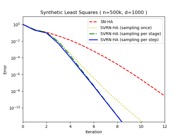
Figure 3: Comparison of three variants of SVRN-HA (alongside SN-HA), depending on how frequently we resample data points used to compute the gradient estimate. We consider three variants of SVRN-HA: (1) sampling once for the entire optimization, (2) sampling once for each full gradient stage (per stage), (3) sampling in each small step (per step).

We next use a simpler and more predictable setting of least squares regression to analyze the trade-offs in convergence for different implementations of SVRN. Here, we observed little difference in convergence behavior when varying $\kappa_{\mathbf{A}}$ (we show results for $\kappa_{\mathbf{A}}=10^{3}$).

Frequency of gradient resampling.

Our theoretical analysis requires that for each small step of SVRN, a fresh sample of components $\psi_{i}$ is used to compute the gradient estimates. However, in Lemma 2 we showed that, after variance reduction, the gradient estimates are accurate with high probability, which suggests that we might be able to reuse previously sampled components. While this technically does not improve the number of required gradient queries, it can substantially reduce the communication cost for some practical implementations. In Figure 3, we investigate how much the convergence rate of SVRN-HA is affected by the frequency of component resampling for the gradient estimates. Recall that in all our experiments, we use a gradient sample size of $m=\lfloor n/\log_{2}(n/d)\rfloor$. We consider the following variants:

1. Sampling once: an extreme policy of sampling one set of components and reusing them for all gradient estimates;

2. Sampling per stage: an intermediate policy of resampling the components after every full gradient computation.

3. Sampling per step: the policy which is used in our theory, i.e., resampling the gradients at every step of the inner loop of the algorithm.

From Figure 3 we conclude that, while all three variants of SVRN-HA converge and are competitive with SN-HA, the extreme policy of sampling once leads to a substantial degradation in convergence rate, whereas sampling per stage and sampling per step perform very similarly. Thus, our overall recommendation is to resample the components at every stage of SVRN-HA, but reuse the sample for the small steps of the algorithm (this is what we used for the EMNIST experiments).

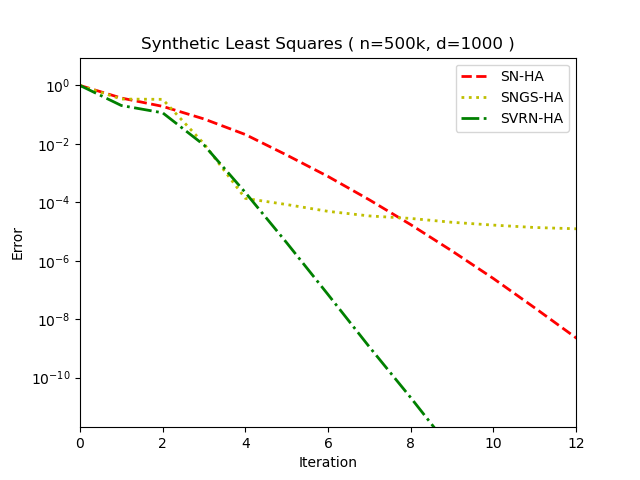
Figure 4: Comparison of SVRN-HA (alongside SN-HA) against Subsampled Newton with Gradient Subsampling (SNGS-HA), which is implemented exactly like SVRN-HA except without the variance-reducing correction.

Effect of variance reduction.

We next investigate the effect of variance reduction on the convergence rate of SVRN. While gradient subsampling has been proposed by many works in the literature on Subsampled Newton, e.g., see [40], these works have shown that the gradient sample size must be gradually increased to retain fast local convergence (which means that after a few iterations, we must use the full gradient). On the other hand, in SVRN, instead of increasing the gradient sample size, we use variance reduction with a fixed sample size, which allows us to retain the accelerated convergence indefinitely. To illustrate this, in Figure 4 we plot how the convergence behavior of our algorithm changes if we take variance reduction out of it. The resulting method is called Subsampled Newton with Gradient Subsampling (SNGS-HA). For this experiment, we resample the gradient estimate at every small step (for both SNGS-HA and SVRN-HA). For the sake of direct comparison, all of the other parameters are retained from SVRN-HA. In particular, one iteration of SNGS-HA corresponds to $\lfloor\log_{2}(n/d)\rfloor$ steps using resampled gradients, and Hessian averaging occurs once every such iteration. As expected, we observe that, while initially converging at a fast rate, eventually SNGS-HA reaches a point where the subsampled gradient estimates are not sufficiently accurate, resulting in a sudden dramatic drop-off in the convergence rate, to the point where the method virtually stops converging altogether. On the other hand, SVRN-HA continues to converge at the same fast rate throughout the optimization procedure without any reduction in performance. This indicates that variance reduction does improve the accuracy of gradient estimates.

Effect of Hessian accuracy.

In our experiments, for both SVRN and SN, we used Hessian averaging [35] to construct the Hessian estimates. This approach is desirable in practice, since it gradually increases the accuracy of the Hessian estimate as we progress in the optimization. As a result, it is more robust to the Hessian sample size and we are guaranteed to reach sufficient accuracy for SVRN to work well. In the following experiment, we take Hessian averaging out of the algorithms to provide a better sense of how the performance of SVRN and SN depends on the accuracy of the provided Hessian estimate. For simplicity, we focus here on least squares, where the Hessian is the same everywhere, so we can simply construct an initial Hessian estimate and then use it throughout the optimization. However, our insights apply more broadly to local convergence for general convex objectives. In Figure 5, we plot the performance of the algorithms as we vary the accuracy of the subsampled Hessian estimates, where $h$ denotes the number of samples used to construct the estimate. In all the results, we keep the gradient sample size and local steps in SVRN fixed as before.

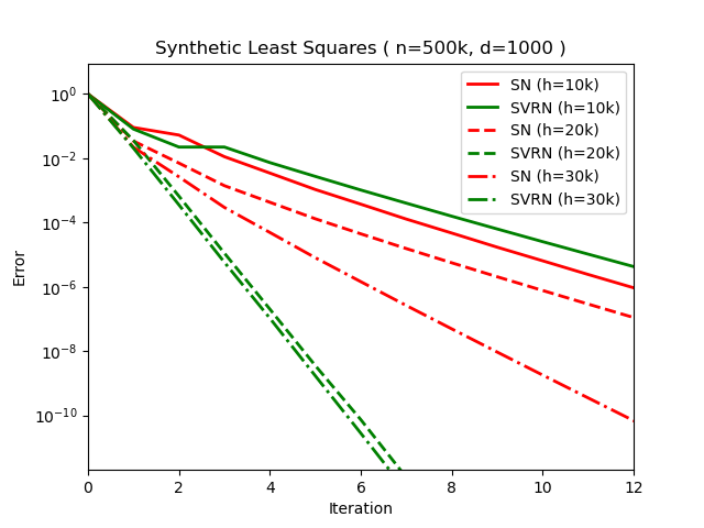
Figure 5: Convergence comparison of SVRN and SN using fixed Hessian estimates (i.e., without Hessian averaging). Here, $h$ denotes the number of Hessian samples used to generate the estimate.

Remarkably, the performance of SVRN is affected by the Hessian accuracy very differently than SN. We observe that SVRN requires a certain level of Hessian accuracy to provide any acceleration over SN. As soon as this level of Hessian accuracy is reached (by increasing the Hessian sample size $h$), the peformance of SVRN quickly jumps to the fast convergence we observed in the other experiments. Further increasing the accuracy no longer appears to affect the convergence rate of SVRN. This is in contrast to SN, whose convergence slowly improves as we increase the Hessian sample size. This intriguing phenomenon is actually fully predicted by our theory for SVRN (together with prior convergence analysis for SN). Our SVRN convergence result (Theorem 1) requires a sufficiently accurate Hessian inverse estimate, but the actual rate of convergence is independent of the Hessian accuracy (only the required number of small steps is affected). We conclude that SVRN is more desirable than SN when we have a small budget for Hessian samples. Ideally, we should use just enough Hessian samples for SVRN to be able to reach the accelerated rate.

Effect of high coherence.

We next analyze the performance of SVRN and SN on a slightly modified least squares task. For this experiment, we modify the data matrix $\mathbf{A}$, by multiplying the $i$th row by $1/\sqrt{g_{i}}$ for each $i$, where $g_{i}$ is an independent random variable distributed according to the Gamma distrution with shape $2$ and scale $1/2$. This is a standard transformation designed to produce a matrix with many rows having a high leverage score. Recall that the leverage score of the $i$th row of $\mathbf{A}$ is defined as $\ell_{i}=\mathbf{a}_{i}^{\scriptscriptstyle{\top}}(\mathbf{A}^{\scriptscriptstyle{\top}}\mathbf{A})^{-1}\mathbf{a}_{i}$, see Appendix A. This can be viewed as affecting the component-wise smoothness of the objective, which hinders subsampling-based estimators of the Hessian and the gradient.

In Figure 6, we illustrate how the performance of SVRN-HA and SN-HA degrades for the high-coherence least squares task, and we also show how this can be addressed by relying on the ideas developed in Appendix A. First, notice that not only is the convergence rate of both SVRN-HA and SN-HA worse on the high-coherence dataset than on the previous least squares examples (e.g., compare with Figure 4), but also, the acceleration coming from variance reduction is drastically reduced to the point of being negligible. The former effect is primarily caused by the fact that uniform Hessian subsampling is much less effective at producing accurate approximations for high-coherence matrices, and this affects both algorithms similarly (we note that one could construct an even more highly coherent matrix, for which these methods would essentially stop converging altogether). The latter effect is the consequence of the fact that gradient subsampling is also adversely affected by high coherence, so it becomes nearly impossible to produce gradient estimates with uniform sampling that would lead to an accelerated rate, even with variance reduction. This corresponds to the regime of $\kappa\geq n$ in our theory, where the accelerated rate of $\tilde{O}(\kappa/n)$ achieved by SVRN is essentially vacuous.

Fortunately, for least squares regression, this phenomenon can be addressed easily. As outlined in Appendix A, we can use one of two strategies: (1) use importance sampling proportional to the leverage scores of $\mathbf{A}$ for both the Hessian and gradient estimates; or (2) precondition the problem using the Randomized Hadamard Transform (RHT) to uniformize all the leverage scores, and then use uniform subsampling. Both of these methods require roughly $O(nd\log n)$ preprocessing cost and eliminate dependence on the condition number for both SVRN-HA and SN-HA. The latter strategy is somewhat more straightforward since it does not require modifying the optimization algorithms, and we apply it here for our high coherence least squares task: we let SVRN-HA-RHT and SN-HA-RHT denote the two optimization algorithms ran after applying the RHT preconditioning to the problem, as described in (5). Note that this not only improves the convergence rate of both methods but also brings back the accelerated rate enjoyed by SVRN-HA in the previous experiments. In fact, our least squares results (Corollary 1 and Lemma 4) can be directly applied to SVRN-HA-RHT, so this method and its accelerated convergence rate of $\tilde{O}(d/n)$ is provably unaffected by any high-coherence matrices.

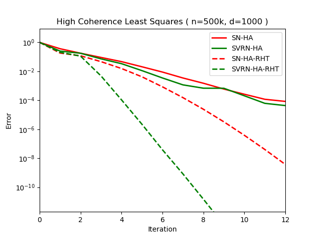
Figure 6: Convergence comparison of SVRN-HA and SN-HA, with and without preconditioning using a Randomized Hadamard Transform (RHT), for a high-coherence least squares dataset.

Appendix C Omitted proofs

C.1 Proof of Lemma 1

This proof is based on standard Newton analysis, and our derivation follows that of [12]. We outline it here for the sake of completeness. We will separately consider the two cases of whether $f$ satisfies Assumption 2 or 3.

Assumption 2 (Lipschitz Hessian).  First, we show that the Hessian at $\mathbf{x}\in U_{f}(\epsilon_{H})$ is an $\epsilon_{H}$-approximation of the Hessian at the optimum $\mathbf{x}^{*}$. Using the shorthand $\mathbf{H}=\nabla^{2}f(\mathbf{x}^{*})$ and the fact that strong convexity (Assumption 1) implies that $\nabla^{2}f(\mathbf{x})\succeq\mu\mathbf{I}$, we have:

$$\|\mathbf{H}^{-1/2}(\nabla^{2}f(\mathbf{x})-\mathbf{H})\mathbf{H}^{-1/2}\|\leq\frac{1}{\mu}\|\nabla^{2}f(\mathbf{x})-\mathbf{H}\|\leq\frac{L}{\mu}\|\mathbf{x}-\mathbf{x}^{*}\|\leq\frac{L}{\mu^{3/2}}\|\mathbf{x}-\mathbf{x}^{*}\|_{\mathbf{H}}\leq\epsilon_{H},$$

which implies that $\nabla^{2}f(\mathbf{x})\approx_{\epsilon_{H}}\!\mathbf{H}$. Then, letting $\Delta=\mathbf{x}-\mathbf{x}^{*}$, we use the standard Newton analysis (similar to [7, Chapter 9.5]) to obtain the rest of the claim:

$$\|\Delta-\nabla^{2}f(\mathbf{x})^{-1}\nabla f(\mathbf{x})\|_{\nabla^{2}f(\mathbf{x})} =\|\nabla^{2}f(\mathbf{x})\Delta-\nabla f(\mathbf{x})\|_{\nabla^{2}f(\mathbf{x})^{-1}}\leq\frac{1}{\sqrt{\mu}}\|\nabla^{2}f(\mathbf{x})\Delta-\nabla f(\mathbf{x})\|$$

$$=\frac{1}{\sqrt{\mu}}\Big{\|}\nabla^{2}f(\mathbf{x})\Delta-\Big{(}\int_{0}^{1}\nabla^{2}f(\mathbf{x}^{*}+z\Delta)dz\Big{)}\Delta\Big{\|}$$

$$\leq\frac{1}{\sqrt{\mu}}\|\Delta\|\cdot\int_{0}^{1}\|\nabla^{2}f(\mathbf{x})-\nabla^{2}f(\mathbf{x}^{*}+z\Delta)\|dz$$

$$\leq\frac{1}{\sqrt{\mu}}\,\frac{L}{2}\|\Delta\|^{2}\leq\frac{L}{2\mu^{3/2}}\|\Delta\|_{\nabla^{2}f(\mathbf{x})}^{2}\leq\epsilon_{H}\,\|\Delta\|_{\nabla^{2}f(\mathbf{x})}.$$

Assumption 3 (Self-concordance).  The fact that $\nabla^{2}f(\mathbf{x})\approx_{\epsilon_{H}}\!\mathbf{H}$ follows from the following property of self-concordant functions [7, Chapter 9.5], which holds when $\|\Delta\|_{\mathbf{H}}<1$, for $\Delta=\mathbf{x}-\mathbf{x}^{*}$:

$$(1-\|\Delta\|_{\mathbf{H}})^{2}\cdot\mathbf{H}\preceq\nabla^{2}f(\mathbf{x})\preceq(1-\|\Delta\|_{\mathbf{H}})^{-2}\cdot\mathbf{H},$$

where we again let $\mathbf{H}=\nabla^{2}f(\mathbf{x}^{*})$. Next, via a similar integral argument as in the Lipschitz case, we can show that for self-concordant functions:

$$\|\Delta-\nabla^{2}f(\mathbf{x})^{-1}\nabla f(\mathbf{x})\|_{\nabla^{2}f(\mathbf{x})}\leq\frac{\|\Delta\|_{\nabla^{2}f(\mathbf{x})}^{2}}{1-\|\Delta\|_{\nabla^{2}f(\mathbf{x})}}\leq\frac{\epsilon_{H}}{2(1-\epsilon_{H})}\cdot\|\Delta\|_{\nabla^{2}f(\mathbf{x})}\leq\epsilon_{H}\cdot\|\Delta\|_{\nabla^{2}f(\mathbf{x})},$$

where we used that $\mathbf{x}\in U_{f}(\epsilon_{H})$ and that $\epsilon_{H}\leq 1/2$.

C.2 Proof of Lemma 2

We use the following standard version of Bernstein’s concentration inequality for random vectors.

Lemma 5 (Corollary 4.1 in [32])

Let $\mathbf{v}_{1},...,\mathbf{v}_{m}\in\mathbb{R}^{d}$ be independent random vectors such that $\mathbb{E}[\mathbf{v}_{i}]=\mathbf{0}$ and $\|\mathbf{v}_{i}\|\leq R$ almost surely. Denote $\sigma^{2}:=\sum_{i=1}^{m}\mathbb{E}\,\|\mathbf{v}_{i}\|^{2}$. Then, for all $t^{2}\geq\sigma^{2}+tR/3$, we have

$$\mathrm{Pr}\bigg{\{}\Big{\|}\sum_{i=1}^{m}\mathbf{v}_{i}\Big{\|}>t\bigg{\}}\leq 28\exp\Big{(}-\frac{t^{2}/2}{\sigma^{2}+tR/3}\Big{)}.$$

We will apply Lemma 5 to $\mathbf{v}_{i}=\nabla\psi_{i}(\mathbf{x})-\nabla\psi_{i}(\mathbf{x}^{*})-\nabla f(\mathbf{x})$. First, observe that $\mathbb{E}\,\nabla\psi_{i}(\mathbf{x})=\nabla f(\mathbf{x})$ and $\mathbb{E}\,\nabla\psi_{i}(\mathbf{x}^{*})=\nabla f(\mathbf{x}^{*})=\mathbf{0}$, so in particular, $\mathbb{E}[\mathbf{v}_{i}]=\mathbf{0}$. Next, since both $\psi_{i}$ and $f$ are $\lambda$-smooth, we have:

$$\|\mathbf{v}_{i}\|^{2} \leq 2\|\nabla\psi_{i}(\mathbf{x})-\nabla\psi_{i}(\mathbf{x}^{*})\|^{2}+2\|\nabla f(\mathbf{x})\|^{2}$$

$$\leq 4\lambda\cdot\big{(}\psi_{i}(\mathbf{x})-\psi_{i}(\mathbf{x}^{*})-(\mathbf{x}-\mathbf{x}^{*})^{\scriptscriptstyle{\top}}\nabla\psi(\mathbf{x}^{*})\big{)}+4\lambda\cdot\big{(}f(\mathbf{x})-f(\mathbf{x}^{*})\big{)}$$

$$\leq 2\lambda^{2}\|\mathbf{x}-\mathbf{x}^{*}\|^{2}+2\lambda^{2}\|\mathbf{x}-\mathbf{x}^{*}\|^{2}=4\lambda^{2}\|\mathbf{x}-\mathbf{x}^{*}\|^{2},$$

where we used that for a $\lambda$-smooth function $g$, we have $\|\nabla g(\mathbf{x})\|^{2}\leq 2\lambda\cdot(g(\mathbf{x})-\min_{\mathbf{x}^{\prime}}g(\mathbf{x}^{\prime}))$ (e.g., see proof of Lemma 1 in [22]), and we applied this inequality to $f$, as well as to $g(\mathbf{x})=\psi_{i}(\mathbf{x})-\psi_{i}(\mathbf{x}^{*})-(\mathbf{x}-\mathbf{x}^{*})^{\scriptscriptstyle{\top}}\nabla\psi(\mathbf{x}^{*})$. To bound the expectation $\mathbb{E}\,\|\mathbf{v}_{i}\|^{2}$, we use the intermediate inequality from the above derivation, obtaining:

$$\mathbb{E}\,\|\mathbf{v}_{i}\|^{2} \leq\mathbb{E}\,\|\nabla\psi_{i}(\mathbf{x})-\nabla\psi_{i}(\mathbf{x}^{*})\|^{2}$$

$$\leq\mathbb{E}\,2\lambda\cdot\big{(}\psi_{i}(\mathbf{x})-\psi_{i}(\mathbf{x}^{*})-(\mathbf{x}-\mathbf{x}^{*})^{\scriptscriptstyle{\top}}\nabla\psi(\mathbf{x}^{*})\big{)}$$

$$=2\lambda\cdot\big{(}f(\mathbf{x})-f(\mathbf{x}^{*})\big{)}.$$

We now use the assumption that $\mathbf{x}\in U_{f}(\epsilon_{H})$, which implies via Lemma 3 that $f(\mathbf{x})-f(\mathbf{x}^{*})\leq(1+\epsilon_{H})\frac{1}{2}\|\mathbf{x}-\mathbf{x}^{*}\|_{\nabla f(\mathbf{x})}^{2}$. Thus, we can use Lemma 5 with $R=2\lambda\|\mathbf{x}-\mathbf{x}^{*}\|$ and $\sigma^{2}=2m\lambda\|\mathbf{x}-\mathbf{x}^{*}\|_{\nabla^{2}f(\mathbf{x})}^{2}$, as well as $\mu$-strong convexity of $f$, obtaining that with probability $1-\delta$,

$$\|\widehat{{\mathbf{g}}}(\mathbf{x})-\widehat{{\mathbf{g}}}(\mathbf{x}^{*})-\nabla f(\mathbf{x})\|_{\nabla^{2}f(\mathbf{x})^{-1}}^{2} \leq\frac{1}{\mu}\Big{\|}\frac{1}{m}\sum_{i=1}^{m}\mathbf{v}_{i}\Big{\|}^{2}$$

$$\leq\frac{C}{\mu}\Big{(}\frac{\sigma^{2}\log(1/\delta)}{m^{2}}+\frac{R^{2}\log^{2}(1/\delta)}{m^{2}}\Big{)}$$

$$\leq\frac{C}{\mu}\bigg{(}\frac{2\lambda\|\mathbf{x}-\mathbf{x}^{*}\|_{\nabla^{2}f(\mathbf{x})}^{2}\log(1/\delta)}{m}+\frac{4\lambda^{2}\|\mathbf{x}-\mathbf{x}^{*}\|^{2}\log^{2}(1/\delta)}{m^{2}}\bigg{)}$$

$$\leq 4C\bigg{(}\frac{\kappa\log(1/\delta)}{m}+\frac{\kappa^{2}\log^{2}(1/\delta)}{m^{2}}\bigg{)}\cdot\|\mathbf{x}-\mathbf{x}^{*}\|_{\nabla^{2}f(\mathbf{x})}^{2}$$

$$\leq 8C\log(1/\delta)\cdot\frac{\kappa}{m}\,\|\mathbf{x}-\mathbf{x}^{*}\|_{\nabla^{2}f(\mathbf{x})}^{2},$$

where in the last step we used the assumption that $m\geq\kappa\log(1/\delta)$.

C.3 Proof of Lemma 3

We use a version of the Quadratic Taylor’s Theorem, as given below.

Lemma 6 (Theorem 3 in Chapter 2.6 of [26]; see also Chapter 2.7 in [21])

Suppose that $f:\mathbb{R}^{d}\rightarrow\mathbb{R}$ has continuous first and second derivatives. Then, for any $\mathbf{a}$ and $\mathbf{v}$, there exists $\theta\in(0,1)$ such that:

$$f(\mathbf{a}+\mathbf{v})=f(\mathbf{a})+\nabla f(\mathbf{a})^{\scriptscriptstyle{\top}}\mathbf{v}+\frac{1}{2}\mathbf{v}^{\scriptscriptstyle{\top}}\nabla^{2}f(\mathbf{a}+\theta\mathbf{v})\mathbf{v}.$$

Applying Talyor’s theorem with $\mathbf{a}=\mathbf{x}^{*}$ and $\mathbf{v}=\mathbf{x}-\mathbf{x}^{*}$, there is a $\mathbf{z}=\mathbf{x}^{*}+\theta(\mathbf{x}-\mathbf{x}^{*})$ such that:

$$f(\mathbf{x})-f(\mathbf{x}^{*})=\frac{1}{2}\|\mathbf{x}-\mathbf{x}^{*}\|_{\nabla^{2}f(\mathbf{z})}^{2},$$

where we use that $\nabla f(\mathbf{x}^{*})=\mathbf{0}$. Since we assumed that $\mathbf{x}\in U_{f}(\epsilon_{H})$, and naturally also $\mathbf{x}^{*}\in U_{f}(\epsilon_{H})$, this means that $\mathbf{z}\in U_{f}(\epsilon_{H})$, given that $U_{f}(\epsilon_{H})$ is convex. Thus, using Lemma 1, we have $\|\mathbf{x}-\mathbf{x}^{*}\|_{\nabla^{2}f(\mathbf{z})}^{2}\approx_{\epsilon_{H}}\|\mathbf{x}-\mathbf{x}^{*}\|_{\nabla^{2}f(\mathbf{x}^{*})}^{2}$.

References

- [1] Nir Ailon and Bernard Chazelle. The fast Johnson–Lindenstrauss transform and approximate nearest neighbors. SIAM Journal on computing, 39(1):302–322, 2009.
- [2] Zeyuan Allen-Zhu. Katyusha: The first direct acceleration of stochastic gradient methods. The Journal of Machine Learning Research, 18(1):8194–8244, 2017.
- [3] Zeyuan Allen-Zhu and Yang Yuan. Improved svrg for non-strongly-convex or sum-of-non-convex objectives. In International conference on machine learning, pages 1080–1089. PMLR, 2016.
- [4] Haim Avron, Petar Maymounkov, and Sivan Toledo. Blendenpik: Supercharging lapack’s least-squares solver. SIAM Journal on Scientific Computing, 32(3):1217–1236, 2010.
- [5] Albert S Berahas, Raghu Bollapragada, and Jorge Nocedal. An investigation of newton-sketch and subsampled newton methods. Optimization Methods and Software, 35(4):661–680, 2020.
- [6] Raghu Bollapragada, Richard H Byrd, and Jorge Nocedal. Exact and inexact subsampled newton methods for optimization. IMA Journal of Numerical Analysis, 39(2), 2018.
- [7] Stephen Boyd and Lieven Vandenberghe. Convex optimization. Cambridge university press, 2004.
- [8] Kenneth L. Clarkson and David P. Woodruff. Low-rank approximation and regression in input sparsity time. J. ACM, 63(6):54:1–54:45, January 2017.
- [9] Gregory Cohen, Saeed Afshar, Jonathan Tapson, and Andre Van Schaik. Emnist: Extending mnist to handwritten letters. In 2017 international joint conference on neural networks (IJCNN), pages 2921–2926. IEEE, 2017.
- [10] Aaron Defazio, Francis Bach, and Simon Lacoste-Julien. Saga: A fast incremental gradient method with support for non-strongly convex composite objectives. Advances in neural information processing systems, 27, 2014.
- [11] Michał Dereziński, Burak Bartan, Mert Pilanci, and Michael W Mahoney. Debiasing distributed second order optimization with surrogate sketching and scaled regularization. In Advances in Neural Information Processing Systems, volume 33, pages 6889–6899, 2020.
- [12] Michał Dereziński, Jonathan Lacotte, Mert Pilanci, and Michael W Mahoney. Newton-LESS: Sparsification without trade-offs for the sketched newton update. Advances in Neural Information Processing Systems, 34, 2021.
- [13] Michał Dereziński, Zhenyu Liao, Edgar Dobriban, and Michael W Mahoney. Sparse sketches with small inversion bias. In Proceedings of the 34th Conference on Learning Theory, 2021.
- [14] Michał Dereziński, Dhruv Mahajan, S. Sathiya Keerthi, S. V. N. Vishwanathan, and Markus Weimer. Batch-expansion training: An efficient optimization framework. In Amos Storkey and Fernando Perez-Cruz, editors, Proceedings of the Twenty-First International Conference on Artificial Intelligence and Statistics, volume 84 of Proceedings of Machine Learning Research, pages 736–744, Playa Blanca, Lanzarote, Canary Islands, 09–11 Apr 2018.
- [15] Michał Dereziński and Michael W Mahoney. Distributed estimation of the inverse hessian by determinantal averaging. In Advances in Neural Information Processing Systems 32, pages 11401–11411. Curran Associates, Inc., 2019.
- [16] Michał Dereziński and Michael W Mahoney. Determinantal point processes in randomized numerical linear algebra. Notices of the American Mathematical Society, 68(1):34–45, 2021.
- [17] Petros Drineas, Malik Magdon-Ismail, Michael W. Mahoney, and David P. Woodruff. Fast approximation of matrix coherence and statistical leverage. J. Mach. Learn. Res., 13(1):3475–3506, December 2012.
- [18] Petros Drineas and Michael W. Mahoney. RandNLA: Randomized numerical linear algebra. Communications of the ACM, 59:80–90, 2016.
- [19] Petros Drineas, Michael W Mahoney, and S Muthukrishnan. Sampling algorithms for regression and applications. In Proceedings of the seventeenth annual ACM-SIAM symposium on Discrete algorithm, pages 1127–1136, 2006.
- [20] Murat A Erdogdu and Andrea Montanari. Convergence rates of sub-sampled Newton methods. Advances in Neural Information Processing Systems, 28:3052–3060, 2015.
- [21] Gerald Folland. Advanced calculus. Upper Saddle River, NJ : Prentice Hall, 2002.
- [22] Roy Frostig, Rong Ge, Sham M Kakade, and Aaron Sidford. Competing with the empirical risk minimizer in a single pass. In Conference on learning theory, pages 728–763. PMLR, 2015.
- [23] Alon Gonen, Francesco Orabona, and Shai Shalev-Shwartz. Solving ridge regression using sketched preconditioned svrg. In International conference on machine learning, pages 1397–1405. PMLR, 2016.
- [24] Robert Gower, Donald Goldfarb, and Peter Richtárik. Stochastic block bfgs: Squeezing more curvature out of data. In International Conference on Machine Learning, pages 1869–1878. PMLR, 2016.
- [25] Robert Gower, Nicolas Le Roux, and Francis Bach. Tracking the gradients using the hessian: A new look at variance reducing stochastic methods. In International Conference on Artificial Intelligence and Statistics, pages 707–715. PMLR, 2018.
- [26] Robert Jerrard. Multivariable calculus. https://www.math.toronto.edu/courses/mat237y1/20189/notes/Contents.html, 2018. Course Notes.
- [27] Rie Johnson and Tong Zhang. Accelerating stochastic gradient descent using predictive variance reduction. Advances in neural information processing systems, 26, 2013.
- [28] Hongzhou Lin, Julien Mairal, and Zaid Harchaoui. A universal catalyst for first-order optimization. Advances in neural information processing systems, 28, 2015.
- [29] Yanli Liu, Fei Feng, and Wotao Yin. Acceleration of svrg and katyusha x by inexact preconditioning. In International Conference on Machine Learning, pages 4003–4012. PMLR, 2019.
- [30] Xiangrui Meng and Michael W. Mahoney. Low-distortion subspace embeddings in input-sparsity time and applications to robust linear regression. In Proceedings of the Forty-fifth Annual ACM Symposium on Theory of Computing, STOC ’13, pages 91–100, New York, NY, USA, 2013. ACM.
- [31] Xiangrui Meng, Michael A Saunders, and Michael W Mahoney. LSRN: A parallel iterative solver for strongly over-or underdetermined systems. SIAM Journal on Scientific Computing, 36(2):C95–C118, 2014.
- [32] Stanislav Minsker. On some extensions of bernstein’s inequality for self-adjoint operators. Statistics & Probability Letters, 127:111–119, 2017.
- [33] Aryan Mokhtari, Mark Eisen, and Alejandro Ribeiro. Iqn: An incremental quasi-newton method with local superlinear convergence rate. SIAM Journal on Optimization, 28(2):1670–1698, 2018.
- [34] Philipp Moritz, Robert Nishihara, and Michael Jordan. A linearly-convergent stochastic l-bfgs algorithm. In Artificial Intelligence and Statistics, pages 249–258. PMLR, 2016.
- [35] Sen Na, Michał Dereziński, and Michael W Mahoney. Hessian averaging in stochastic newton methods achieves superlinear convergence. arXiv preprint arXiv:2204.09266, 2022.
- [36] Jelani Nelson and Huy L. Nguyên. Osnap: Faster numerical linear algebra algorithms via sparser subspace embeddings. In Proceedings of the 2013 IEEE 54th Annual Symposium on Foundations of Computer Science, FOCS ’13, pages 117–126, Washington, DC, USA, 2013. IEEE Computer Society.
- [37] Mert Pilanci and Martin J Wainwright. Iterative hessian sketch: Fast and accurate solution approximation for constrained least-squares. The Journal of Machine Learning Research, 17(1):1842–1879, 2016.
- [38] Mert Pilanci and Martin J Wainwright. Newton sketch: A near linear-time optimization algorithm with linear-quadratic convergence. SIAM Journal on Optimization, 27(1):205–245, 2017.
- [39] Vladimir Rokhlin and Mark Tygert. A fast randomized algorithm for overdetermined linear least-squares regression. Proceedings of the National Academy of Sciences, 105(36):13212–13217, 2008.
- [40] Farbod Roosta-Khorasani and Michael W Mahoney. Sub-sampled newton methods. Mathematical Programming, 174(1):293–326, 2019.
- [41] Nicolas Roux, Mark Schmidt, and Francis Bach. A stochastic gradient method with an exponential convergence rate for finite training sets. Advances in neural information processing systems, 25, 2012.
- [42] Shai Shalev-Shwartz and Tong Zhang. Stochastic dual coordinate ascent methods for regularized loss minimization. Journal of Machine Learning Research, 14(2), 2013.
- [43] David P Woodruff. Sketching as a tool for numerical linear algebra. Foundations and Trends® in Theoretical Computer Science, 10(1–2):1–157, 2014.
- [44] Jiyan Yang, Yin-Lam Chow, Christopher Ré, and Michael W Mahoney. Weighted sgd for lp regression with randomized preconditioning. The Journal of Machine Learning Research, 18(1):7811–7853, 2017.
- [45] Junyu Zhang, Lin Xiao, and Shuzhong Zhang. Adaptive stochastic variance reduction for subsampled newton method with cubic regularization. INFORMS Journal on Optimization, 4(1):45–64, 2022.
- [46] Dongruo Zhou, Pan Xu, and Quanquan Gu. Stochastic variance-reduced cubic regularization methods. J. Mach. Learn. Res., 20(134):1–47, 2019.