Crust Macrofracturing as the Evidence of the Last Deglaciation

Abstract

Machine learning methods were applied to reconsider the results of several passive seismic experiments in Finland. We created datasets from different stages of the receiver function technique and processed them with one of basic machine learning algorithms. All the results were obtained uniformly with the k-nearest neighbors algorithm. The first result is the Moho depth map of the region. Another result is the delineation of the near-surface low $S$-wave velocity layer. There are three such areas in the Northern, Southern, and central parts of the region. The low $S$-wave velocity in the Northern and Southern areas can be linked to the geological structure. However, we attribute the central low $S$-wave velocity area to a large number of water-saturated cracks in the upper 1-5 km. Analysis of the structure of this area leads us to the conclusion that macrofracturing was caused by the last deglaciation.

1 Introduction

Passive seismic experiments SVEKALAPKO (Bock et al., 2001) and POLENET/LAPNET (Kozlovskaya et al., 2006) spurred a large number of research activities that targeted the lithosphere structure of the northern part of the Baltic Shield (Bruneton et al., 2002; Alinaghi et al., 2003; Aleshin et al., 2006; Vecsey et al., 2007; Kozlovskaya et al., 2008; Uski et al., 2011; Grad and Tiira, 2012; Silvennoinen et al., 2014; Vinnik et al., 2016). A significant part of these studies is based on the receiver function technique (Alinaghi et al., 2003; Aleshin et al., 2006; Kozlovskaya et al., 2008; Grad and Tiira, 2012; Vinnik et al., 2016). With data from a wide network of seismic stations across the region, this method yielded several important results on the structure of the mantle of northern and southern Finland (Alinaghi et al., 2003; Frassetto and Thybo, 2013; Vinnik et al., 2016), and played a key role in the implementation of a three-dimensional seismic model of central and southern Finland (Kozlovskaya et al., 2008). An important structural feature of the region is the presence of a thin surface layer with low shear wave velocities Vs. The layer thickness varies around 1 km, the Vs values are down to 40 percent less than the average over the crust (Aleshin et al., 2006). The presence of this layer was first noted in (Pedersen and Campillo, 1991; Grad and Luosto, 1992; Grad and LUOSTO, 1994) in the study of the seismic surface wave attenuation. They reveal not only low values of $S$-wave velocity in the shallow crust but also low values of seismic quality factor (Q-factor), which increase rapidly down to the depth of about 1 km. According to Grad et al. (1998), the Q-factor is suitable to differentiate the Archean and the Proterozoic crust of the Fennoscandian Shield. In Grad and Luosto (1992) showed that the increased density of cracks provide for lower Q-factor for the top 1 km of the crust. This explains the low $S$-wave velocity. The presence of the low $S$-wave velocity surface layer (LVSL) was confirmed later in Aleshin et al. (2006). However, Kozlovskaya et al. (2008) have shown that the presence of such a layer is independent of the age of the rocks, it is present in a significant part of both Archean and Proterozoic regions. The research of the Moho shape adopts the results of our previous studies in the SVEKALAPKO and POLENET/LAPNET projects (Aleshin et al., 2006; Kozlovskaya et al., 2008; Silvennoinen et al., 2014) supplemented by data from earlier research (Dricker et al., 1996; Aleshin et al., 2019) (see Code Availability section for this data). Additionally, we adopted 1D profiles to construct the 3D seismic image in the arias of interest. We had a relatively small amount of input data. The spline interpolation like in (Horspool et al., 2006) or kriging technique as described in (Kozlovskaya et al., 2008) can not be considered optimal in this kind of problem. Instead, we preferred to use a machine-learning approach and chose the k-nearest neighbors (kNN) algorithm for its simplicity. One more reason to choose kNN is the data behind the analysis as it consists of separate sets of three different data types. The first one is the “yes-or-no” presence of the converted phase right after the $P$-wave arrival in the receiver function’s waveform. The second type is a series of $S$-wave velocity vs. depth pairs. The third type is crust thickness beneath the stations. Universally, the machine-learning approach allows us to process all of these types. In the “Data” and “Method” sections we described the input dataset and covered the processing algorithm features, correspondingly. We applied the method to the Moho depth data in the section “Moho Boundary Shape”. Notably, the results appeared to be in good alignment with previous works on the Moho shape of this particular region. In the next section, we applied the machine learning approach to locate and describe the structure of the LVSL regions. In the “Discussion” section we argue in favor of post-glacial rebound as the origin of the low $S$-velocity layer in central Finland.

2 Data

For our analysis, we predominantly utilized the results of the receiver function study of passive seismic experiments data, namely SVEKALAPKO and POLENET/LAPNET. Additionally, we used the results of the previous receiver function study for stations LVZ and APA (Dricker et al., 1996); PITK and KEMI (Aleshin et al., 2019). Finally, we turned to account for the models derived from wide-angle seismic experiments (Janik et al., 2007, 2009).

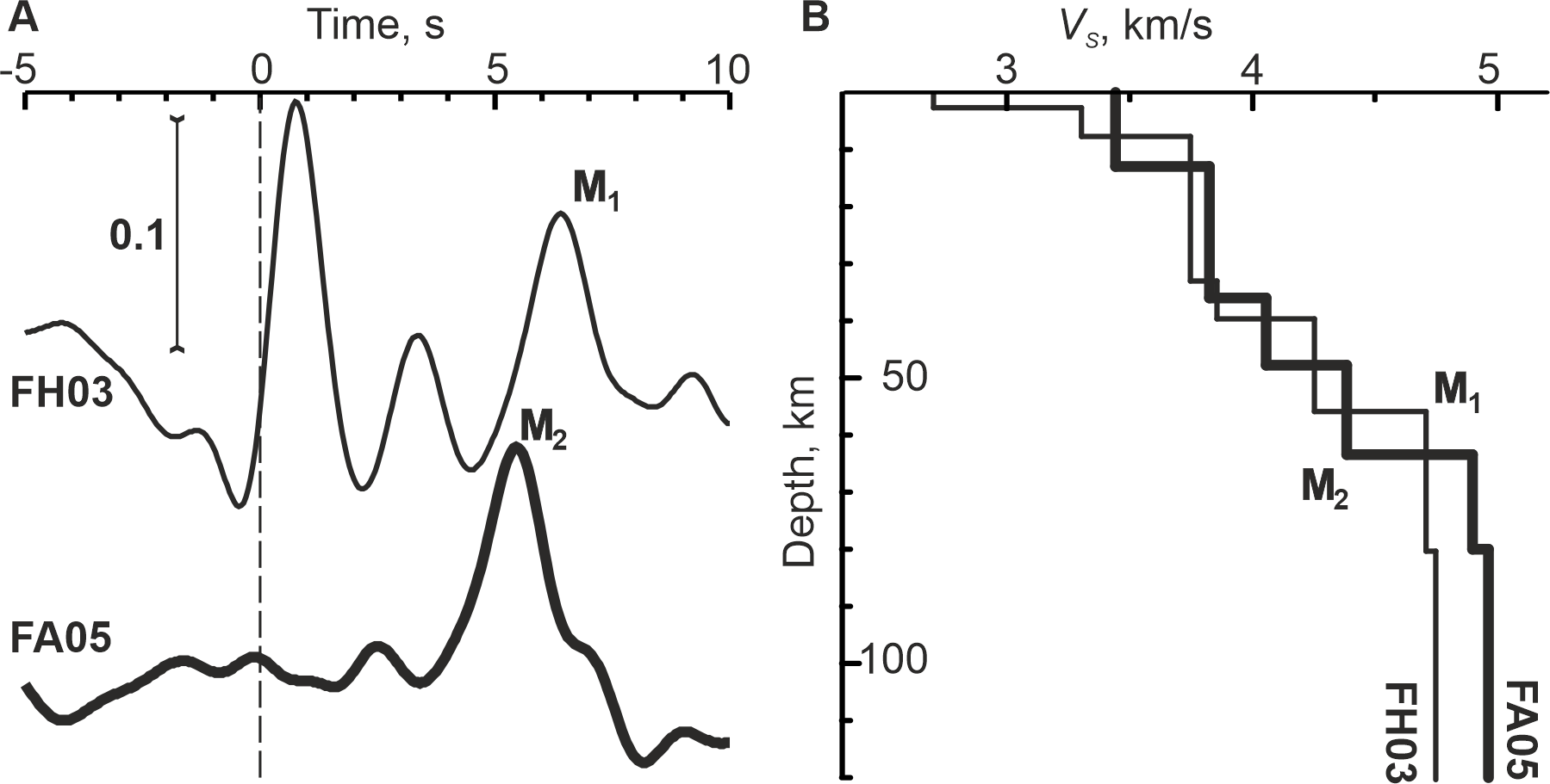
Figure 1: A. Receiver function waveforms of two SVEKALAPKO stations, FH03 (thin line) and FA05 (thick line). FH03 waveform shows clear arrival of the converted phase near the first second after the $P$-wave arrival. This indicates the $S$-velocity jump immediately beneath the station. FA05 doesn’t show such a phase. The letters M₁ and M₂ pick to the Moho border phase. B. Corresponding 1D $S$-velocity profiles obtained through the receiver function inversion (Kozlovskaya et al., 2008). The Moho borders are pointed with the letters M₁ and M₂.

The LVSL under the station is manifested by the strong converted phase arriving within the first seconds after the main $P$-wave. Such a phase is clearly seen on the receiver function waveform (Figure 1, panel A, the FH03 station). We used it to construct the first dataset (dataset “A”) that represents the spatial distribution of the LVSL. Dataset members consist of the station name, location, and logical condition of whether the LVSL is present or not. A few additional dataset members were included from the models derived from wide-angle seismic experiments (Janik et al., 2007, 2009). It was not possible to draw a definite conclusion on the absence or existence of the LVSL under the stations FB11, FD07, LP11, FJ01, LP61, ARE0, LP75. These points were excluded from the dataset. As a result of the analysis, we obtained a set of points with the given values of the Boolean type. The dataset “A” enables us to compute the probability of the LVSL presence at an arbitrary point. To get more details on the structure we require a spatial distribution of elastic parameters. We have obtained it from the 1D $S$-velocity profiles by joint inversion of $P$-receiver functions and surface wave dispersion. Those profiles were adopted from (Kozlovskaya et al., 2008). For the sake of convenience, we quantized the original layered models with 0.1 km step. The choice of the step is more or less volitional. The lower step limit is determined by computation time and complexity. The upper step boundary is limited to the thickness of the thinnest layer across all stations, which appeared to be 0.7 km for our case. Therefore, we’ve got a second dataset, “B”. It contains the station name, location (latitude, longitude? and depth), and the corresponding $S$-velocity. Members of the dataset are irregularly spatially distributed. 1D $S$-velocity profile also provides for determining the Moho depth under the station (see fig. 1, panel B). POLENET/LAPNET (Silvennoinen et al., 2014) and SVEKALAPKO (Kozlovskaya et al., 2008) projects used the same approach to determine the Moho depth. Additionally, the Moho depth for stations LVZ, APA, and PETK, KEMI were adopted from (Dricker et al., 1996) and (Aleshin et al., 2019), respectively. Numerical values of the Moho depth for all the stations are unified into the third type dataset “C”. We used this dataset to construct the Moho depth map.

3 Method

At this point, we have three separate datasets with different types of data: two-dimensional logical values (dataset “A”), three-dimensional floating-point values (dataset “B”), and two-dimensional floating-point values (dataset “C”). We need to obtain the synthetic value for all types of data in datasets at an arbitrary location and depth, where applicable, we opted for using machine-learning methods to do this universally. To perform this task we have to, firstly, define the distance rules for each type of data. For data in dataset “A” and “C”, we can utilize the orthodrome (the geodetic line length). However, due to three-dimensional data in the dataset “B”, the cartesian distance is more convenient. Because the region of interest is quite small we switched from geographical latitude $\phi$ and longitude $\lambda$ to a local Cartesian coordinate system $(x,y)$ using approximate formulae

$$x=2\pi R_{E}(\lambda-\lambda_{1})\cos{\phi_{C}}/360;y=2\pi R_{E}(\phi-\phi_{1})/360;\phi_{C}=(\phi_{2}-\phi_{1})/2;$$ (1)

Here ${R_{E}}$ is the Earth’s radius, $\phi_{1}$, $\phi_{2}$ are the minimal and the maximal latitudinal boundaries of the region, correspondingly; $\lambda_{1}$ is the minimal longitude. Also, the station elevation was set to be zero as we did not include the terrain features into the consideration. There is no prominent influence of the simplifications on the conclusion; we used that due to convenience only. Thus, the distance between two points $\vec{r_{i}}=\{x_{i},y_{i},z_{i}\}$ and $\vec{r_{j}}=\{x_{j},y_{j},z_{j}\}$ was defined as

$$R(\eta;|\vec{r_{i}}-\vec{r_{j}}|=\sqrt{\eta^{2}(z_{j}-z_{i})^{2}+(x_{j}-x_{i})^{2}+(y_{j}-y_{i})^{2}}.$$ (2)

$Z$-axis is assumed normal to the horizontal plane $(x,y)$ plane and zeroes at sea level. The meaning of the scaling factor $\eta$ will be explained later.

As soon as we have defined the distance we should choose a formal mathematical model (algorithm) to be able to calculate the target value for any given location. In general, the algorithm contains a few inner tuning parameters. We can fix them with the input data (the algorithm learning). We’ve chosen the kNN-algorithm, one of the basic machine-learning algorithms. The kNN does not imply any preliminary training procedure. It is evaluated only to predict the target value $F$ at the given location $\vec{r}$ by the set of known values $\\ {f_{i}\\ }$ at given points $\vec{r_{i}}$

$$F=F(\eta,K;\vec{r})=\sum_{i=1}^{K}w(\rho_{i})f_{i}(\vec{r_{i}})/\sum_{j=1}^{K}w(\rho_{j}),\rho_{i}=R(\eta;|\vec{r}-\vec{r_{i}}|).$$ (3)

Here $w(\rho_{i})$ is the weight function that depends on the distance from the current point $\vec{r}$ to the location of the $i$-th dataset member. The summation is performed over the $K$ dataset members closest to the point $\vec{r}$. Usually, the weight function is chosen in the form of a power law:

$$w(\rho_{i})~{}1/\rho_{i}^{\alpha},\alpha>0.$$ (4)

In this paper, we used this law with the value $\alpha=1$. The kNN -algorithm is called a lazy learner because it implies no separate training process. In this algorithm, the dataset is stored in the memory in a certain spatial order based on the distance (2). Formula (3) shows that inner parameters of the algorithm are just $K$ points of the input data nearest to a given position. The computational consumption originates from the search of the members closest to the given point. The complexity of the brute force selection from $N$ elements is about $O(N)$, which is quite inefficient. However, if the data is stored using the binary space partitioning (BSP) scheme the complexity can be reduced to $O(\log N)$. In our work, we used NumPy (Harris et al., 2020) arrays to store the data, which enabled hassle-free k-d tree-like BSP or ball-tree storage organization.

Along with inner parameters, the algorithm used in machine-learning often has hyperparameters, which do not change during training. In our case, these hyperparameters are the number of nearest neighbors $K$ and scale factor $\eta$ from (2). We chose to determine the optimal values of $K$ (and $\eta$ for dataset “B”) using the cross-validation technique (Hastie et al., 2009). The main idea is to split the input data into training and validation blocks. Training blocks are used to fit the internal parameters of the model. Then, the trained model is used to predict the data of the validation block. The comparison of the predicted data and the validation data is used to estimate the training quality.

Within the actual implementation, the initial set is to split into $p$ blocks, which we will call folds, each of the same size. Each fold is consistently served as a validation block, and the remaining $p-1$ folds act as the training blocks. The main advantage of this strategy is that each piece of data is used both for training and for quality control. There are a lot of strategies for splitting data. For dataset B we chose $p=5$ (see below). In problems with a lack of data, that is the case for datasets “A” and “C”, the value of $p$ is appropriate to be chosen equal to the number of members of the source dataset so that each fold contains just a single point. This strategy is called Leave-on-Out. To estimate the training quality, we have to define the quality function. In regression analysis one of the simplest choices is a mean squared difference between the values calculated from the training block and the corresponding samples in the validation block. Essentially, this metric is a measure of the mean interpolation error. We have chosen such a quality function

$$\mu(K,\eta)=\sqrt{(1/N)\sum_{p=1}^{P}\sum_{l=1}^{L}(F(\eta,K;\vec{r_{l}})-f_{l})^{2}}$$ (5)

to determine hyperparameters $K$ or $K$, $\eta$ in the Moho boundary shape (dataset “C”) and $S$-velocity 3D-model problems (dataset “B”), correspondingly. However, this metric is unsuitable for the calculation of areas covered with a low $S$-velocity layer (dataset “A”). For this problem, we have to formulate the task as a binary classification problem. Within this classification, we divide all the points into two classes. Let the point belong to class 1 if the low $S$-velocity layer at the location of the point exists and to class 0 otherwise. Therefore, our goal is to compute the probabilities that a given point on the surface belongs to class 1 or class 0. In this setting, receiver operating characteristic (ROC) is commonly employed. The ROC curve is created by plotting the true positive rate (probability of detection) versus the false positive rate (probability of false alarm) generated by the binary classifier. The area under the curve (AUC) gives a measure of the classifier quality (more detail can be read elsewhere, (Fawcett, 2006)).The rest of the calculation details are the dataset specific and will be described later.

4 Moho Boundary Shape

For this region, the depth to the seismic Mohorovicic discontinuity approximately equals the compositional crust-mantle boundary. The shape of the Moho boundary with receiver function technique was previously studied for several areas in the region: Kola in Kosarev et al. (1987), Southern Finland in Alinaghi et al. (2003); Kozlovskaya et al. (2008); Grad and Tiira (2012), Northern Finland in Silvennoinen et al. (2014). In a series of works the Moho was investigated with controlled source seismic experiments Grad and Luosto (1992); Janik et al. (2007); Uski et al. (2011). In Grad and Tiira (2012); Uski et al. (2011) the crust thickness was studied as part of the European lithosphere structure. In the paper by Silvennoinen et al. (2014), the topography of the Moho under the northern part of Finland was drawn by a joint interpretation of the receiver function and controlled source experiments. In our paper, however, we only use the data obtained with the receiver function technique. We opted for this limitation because as shown in Silvennoinen et al. (2014) the Moho boundary estimated from the receiver function may differ from that of a controlled source experiment. Several reasons can explain this difference. In the controlled source approach the Moho depth is obtained by $P$-waves in most cases, while the receiver function utilizes $P$- or $S$-waves from teleseismic sources converted at the Moho. Also, the frequency content of the signal from teleseismic source data is rather distinct from that in near-vertical reflection, wide-angle reflection, and refraction experiments. Furthermore, rays in both the near-vertical setup and the receiver function are sub-vertical apart from the wide-angle approach. The other reasons are region-specific. In the southern part of the region, the lowermost part of the crust has a high-velocity layer (Janik et al., 2007) that masks the high-velocity contrast at the Moho for $P$-wave (Janik et al., 2009). Also, there is a tangible seismic anisotropy in the upper mantle (Vecsey et al., 2007; Vinnik et al., 2016; Yanovskaya et al., 2019) that causes the discrepancy in sub-lateral and sub-vertical $P$-wave travel times. The number of nearest neighbors $K$ is only one hyperparameter in the Moho boundary shape problem. To determine an optimal value of $K$ we adopted the Leave-one-Out cross-validation procedure. We used the quality function (5) (we set $\eta$ = 0). The optimal value of $K=4$ minimizes the functional (see fig. 2). The corresponding mean interpolation error is 3.7 km.

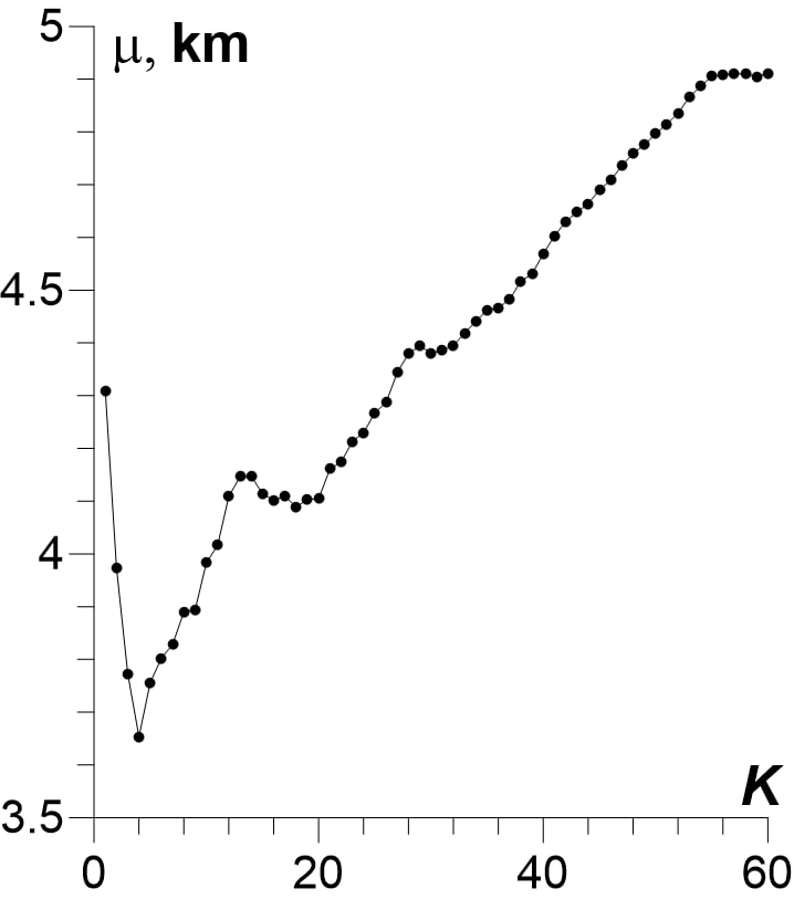
Figure 2: The plot of the quality function (5) versus the number of nearest neighbors $K$ derived from the Moho boundary depth dataset.

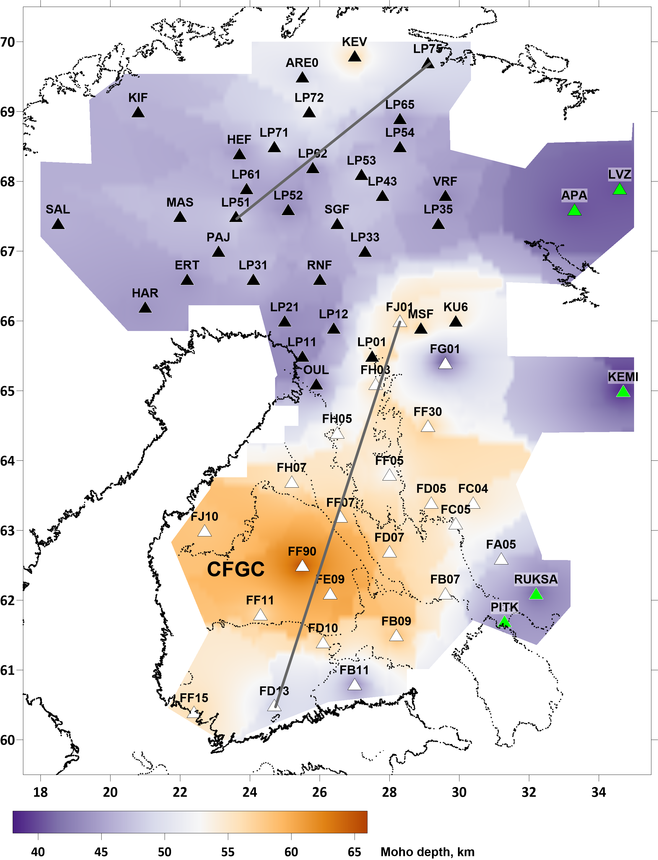
Figure 3: Depth to the Moho boundary. Colored triangles mark the positions of the input points. The color of the symbols corresponds to the source used: black — Silvennoinen et al. (2014); white — Kozlovskaya et al. (2008), green — Dricker et al. (1996); Aleshin et al. (2006, 2019). The abbreviation “CFGC” means Central Finnish Granitoid Complex.

The map in Fig. 3 depicts the depth to the Moho boundary, red —– data from this study. The map was constructed with formulas (1),(2),(3) where $K=4$. The maximum thickness of the crust appears to be in the center of the southern part of the region which corresponds to the results described in Alinaghi et al. (2003); Kozlovskaya et al. (2008); Silvennoinen et al. (2014). Additionally, there is a correlation of the Moho boundary with the Central Finnish Granitoid Complex shapes, which is also discussed in cited papers.

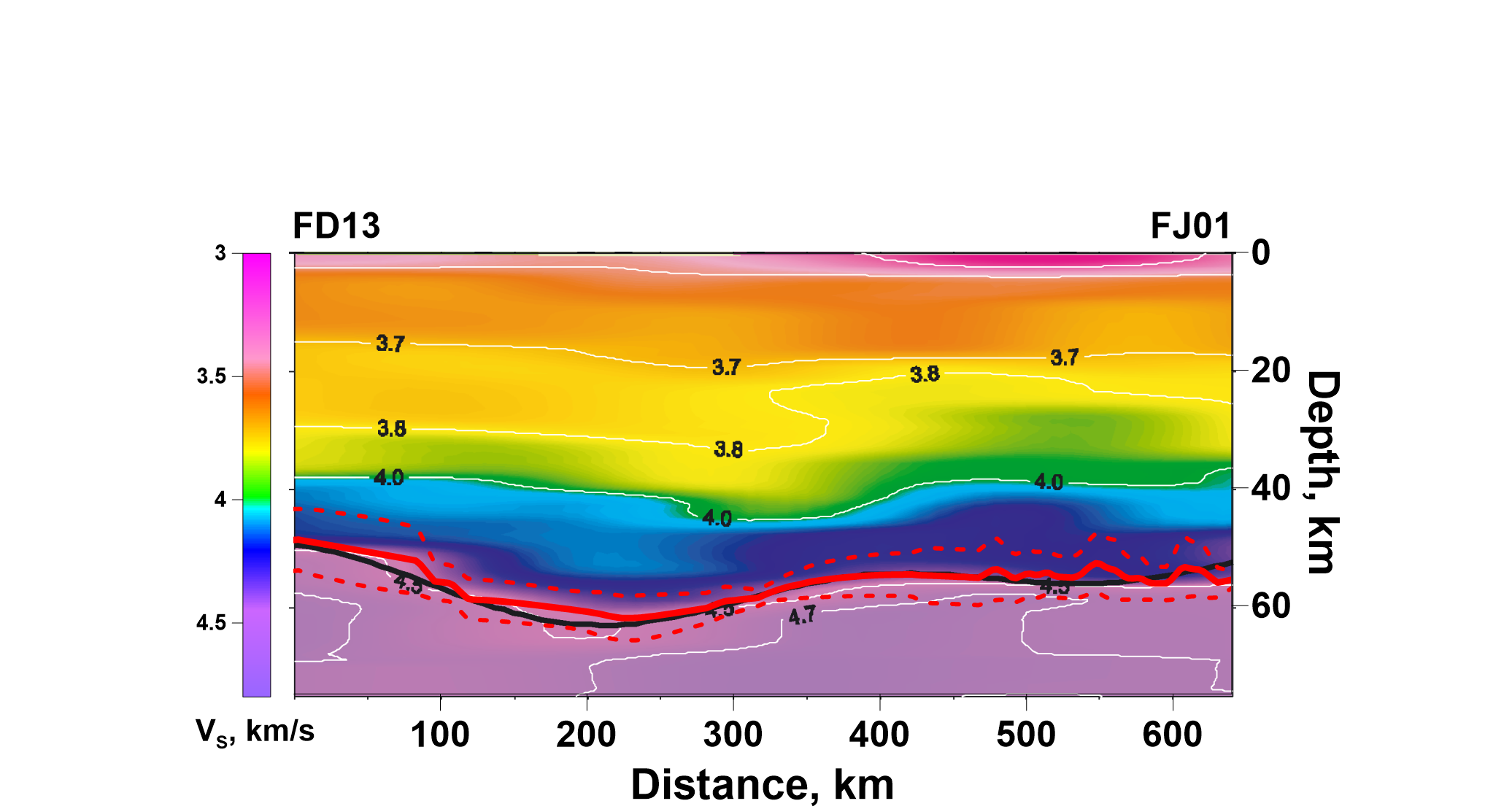
Figure 4: Depth to Moho along with the FD13-FJ01 profile. Black and red lines mark a cross-section of the Moho shape obtained with the kriging technique and the machine learning kNN method, correspondingly; red dashed lines show the kNN interpolation errors. The line oscillations at distances of 550-600 km are likely due to erratic data for station FG01.

Fig. 4 shows the $V_{S}$-profile along FD13-FJ01. The black line marks the Moho depth obtained in Kozlovskaya et al. (2008) with the kriging technique. The solid red line denotes the Moho boundary obtained in this study with the kNN approach. Both lines agree well, showing good consistency among the approaches. Dashed red lines show interpolation error intervals. The map (Fig. 3) and the profile (Fig. 4) reveal the crust thickness anomaly under station FG01. The same was noted by Kozlovskaya et al. (2008). It is worth noting that interpolation misfit surges in the vicinity of FG01, hitting values times the mean error. Thus, we lack the confidence to conclude on the Moho depth there.

5 Map of the low $S$-velocity Layer in the uppermost crust

Now, we can apply the machine learning approach to dataset “A” to build a map of the LVSL coverage in the region. At first, we have to determine the optimal number of nearest neighbors $K$. We used the ROC-AUC metric and applied the Leave-one-Out strategy for cross-validation, similar to the Moho shape calculation. The larger ROC-AUC value corresponds to the better classification model. From the left panel of 5, one can see that the optimal number of nearest neighbors is reached at $K=4$. The shape of ROC at this value is plotted on the right panel.

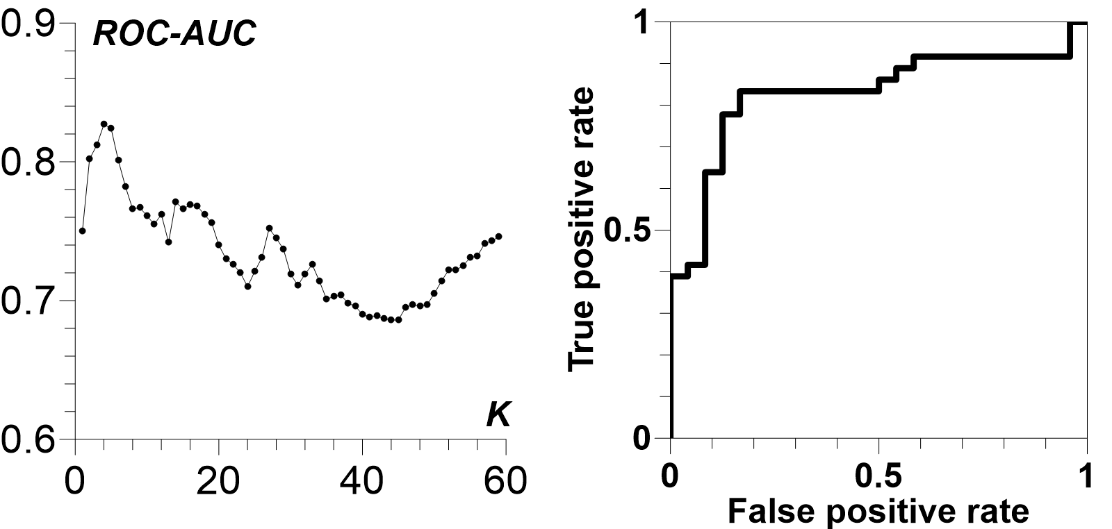
Figure 5: The plot of the ROC-AUC versus the number of nearest neighbors $K$ (left). The plot of ROC for the optimal value of $K=4$ (right).

To construct the map of LVSL from the dataset “A” we substituted $\eta=0$ and $K=4$ in formulae 1, 2. The calculation was performed at nodes $\vec{r_{n}}$ of the regular surface grid. By the definition, every member of the input dataset “A” is either 0 or 1. It leads to the function $F_{n}=F(K,\vec{r_{n}})$ from formula (5) is constrained to $0\leq F_{\alpha}\leq 1$. Thus $F_{n}$ might be treated as the probability of the presence of the LVSL at the given point $\vec{r_{n}}$. To perform the final classification we had chosen two threshold values $t_{0}$ and $t_{1}$. Whether the $F_{n}$ was less than $t_{0}=0.4$ we concluded that there was no LVSL at the point $\vec{r_{n}}$. As a result, the point was classified as class “0”. Otherwise, when $F_{n}$ exceeded $t_{1}=0.6$ we decided that there was an LVSL at this pint, and $\vec{r}_{n}$ was classified as class “1”. The interim values of $F_{n}$ that comply with $(t_{0}<F_{n}<t_{1})$ remained unclassified and formed the “buffer zones” between two classes.

The map obtained is shown in Fig. 6. The map contains three separate LVSL areas in the northern, central, and southern parts of Finland. Stations excluded from the analysis are mostly located near the borders of those areas like FB11, FD07, LP61, or near the outer border of the region like ARE0, LP75. Such distribution explains partly the difficulties of the initial classification. With new results, we can suspect the existence of the LVSL under the station LP61. There appears to be no such layer under the stations LP11, FJ01, and in point HT. The stations FD07 and FB11 are located inside the “buffer zones” so we can not decide the LVSL under these points.

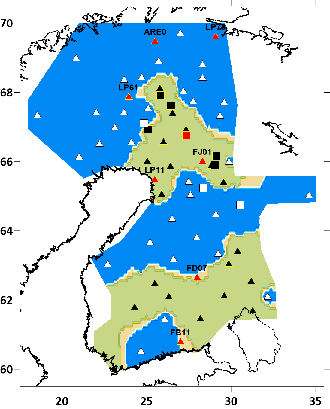
Figure 6: Map of the low-velocity surface layer calculated from the dataset “A”. Areas in which the probability of the presence of the LVSL exceeds 60% are colored in blue. Olive shaded areas denote the probability is less than 40%. Triangles indicate the position of seismic stations and squares indicate the points from wide-angle experiments. They are white or black, depending on the presence or absence of the LVSL at the point, respectively. Initially excluded points are marked red.

The southern and northern LVSL areas could be linked to the geology: the metamorphosis of bedrock and the presence of Paleozoic sedimentary rocks atop the archean basement, respectively. In the central part of Finland, the LSLV can be explained with neither the composition nor age of the rocks. As seen in Fig. 6 the LVSL area in central Finland covers both the Archean and Proterozoic rocks. The origin of the layer should be discussed separately. But before that, we used dataset “B” to highlight the structure under this area.

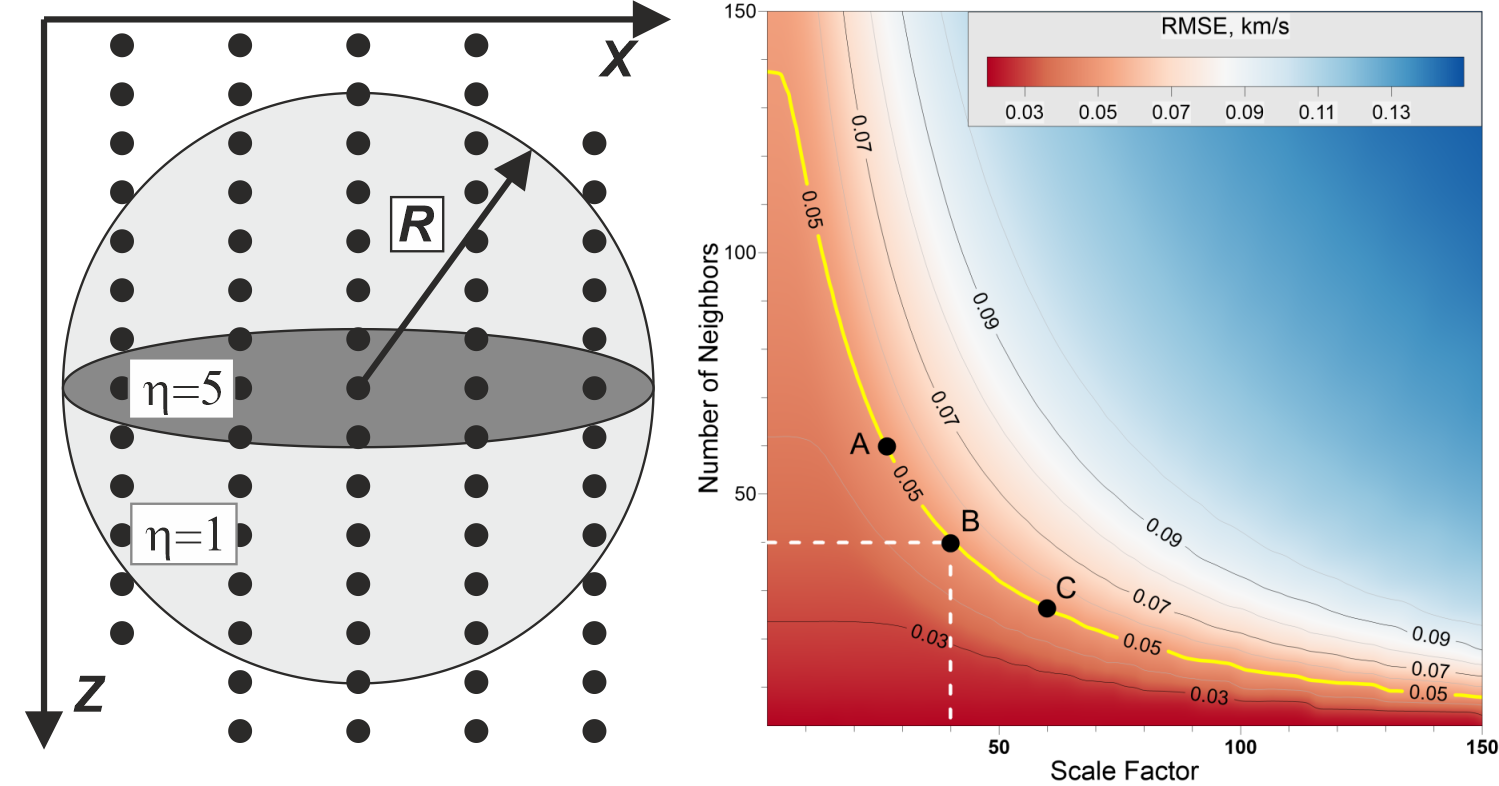
Figure 7: Left: Illustration of the role of scale factor. Right: plot of root-mean-square deviation (formula (5)) for the different values of $K$ and $\eta$.

We have to mention that when we quantized the 1D $S$-velocity profiles we got vertical distances between the points of the same profile much smaller than distances between the stations. Here, to illustrate this issue we would stick with the alternative formulation of kNN where the term “nearest neighbors” assumes all the points inside the sphere of radius R around the given position, see Fig. 7, left. This corresponds to set $\eta=1$ in the formula (2). With moderate R the nearest points would originate from the same profile. The issue could be solved by using the ellipsoid instead of the sphere and setting $\eta>1$. We used a fixed the nearest neighbor number $K$ instead of the radius of the sphere $R$ and the factor controls the $Z$-axis scaling. To determine the optimal $K$ and $\eta$ we used the cross-validation technique for dataset “C”. The dataset “C” has quite a large number of points so we’ve split it into 5 folds of approximately 8000 points each. The quality function $\mu(K,\eta)$ calculated for $K=1,2,...,150$ and $\eta=1,2,...,150$ is shown on Fig. 7, right. Such a distribution is intrinsic to concurrent optimization problems, as seen in, for example, Chiu et al. (2009). Optimal pairs of $K$ and $\eta$ are located where the function $\mu(K,\eta)$ is minimal. These values of $\mu$ are placed at the axes origin on Fig. 7, right. However, this isn’t the case in our problem because picking such low values will lead to very low K and $\eta$ and subsequently to an overinterpretation. Larger values of $K$ and $\eta$ correspond to smoother interpolation results, and to larger $\mu(K,\eta)$. Meanwhile, the error of interpretation cannot exceed the error of the receiver function method, which is typically about 0.1 km/s. Overcauteously, we chose 0.05 km/s for the $\mu(K,\eta)$. This level provides for the optimal pairs of $K$ and $\eta$. For example, picking points A, B, and C from Fig. 7, right net visually equivalent results. So we picked point B, which is the closest to the origin. Such a choice is obvious for multi-objective optimization problems Chiu et al. (2009). We visualized the horizontal section of the $S$-wave velocity at the surface level ($z=0$), see Fig. 8, left. The low velocity region matches the probabilities computed with dataset “A” well. There are strong $S$-velocity variations of the LVSL in archean, proterozoic, and transition regions. We can speculate that the thickness of the LVSL could depend on rock composition, however, investigation of this dependency is out of the scope of the current work. We also imply that the $S$-velocity depends on the amount of rock fracturing and water saturation.

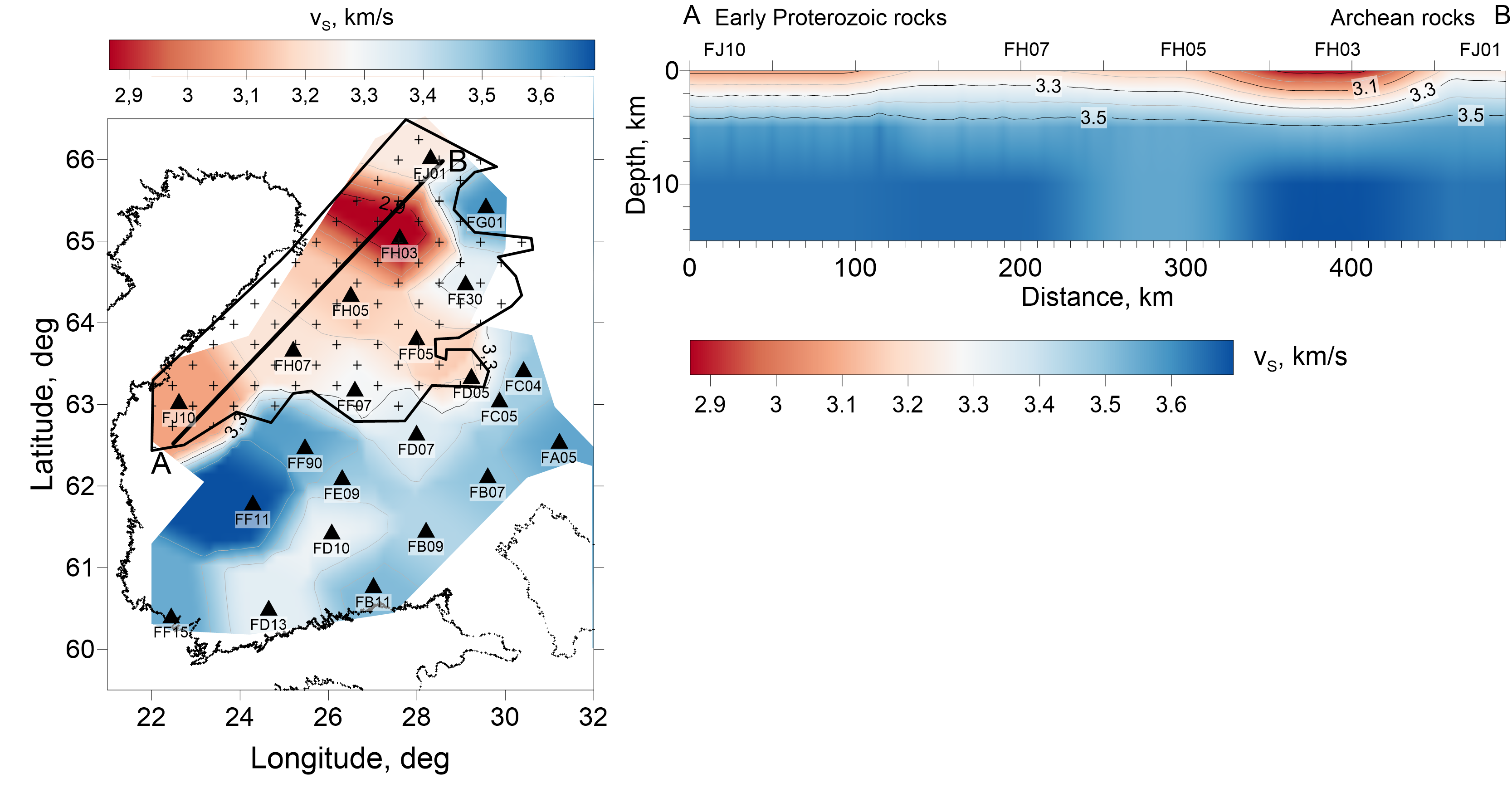
Figure 8: Left: Velocity map of $S$-waves at the surface. Plus-marked (“+”) area matches the central LVSL-area on Fig. 6. Right: vertical section of the $S$-wave velocity of AB profile.

6 Discussion

In our study, we do not make a particular interpretation of $S$-wave velocity values of the low $S$-velocity layer in the uppermost crust. The most interesting fact is that this layer has been revealed both in Archean and Proterozoic areas and it is existing in bedrock units with different compositions. Moreover, it is not correlating with the rock units composed of low-velocity rocks, like granites. For example, the layer is not detected in the Central Finland Granitoid Complex. Therefore, its origin seems to be not dependent on the tectonic age or composition of the bedrock and rock fracturing is the main factor responsible for low velocities. On the other hand, this layer is not distributed uniformly around the Fennoscandia and it is present in several large-scale areas indicated by dark blue in Fig. 8. These two features (e.g. absence of correlation with tectonic age and rock composition and systematic distribution in large-scale areas) need to be explained. In our study, we used the converted waves with dominating periods of 2 s, which means that the wave is averaging fractures of different scales up to 1 km. Such large-scale fractures reaching the depth of 1 km could not form due to rock weathering, but rather due to some large-scale processes. One of the explanations of this layer could be that it has been formed due to the processes related to multiple episodes of deglaciation of the Fennoscandian Shield. Relation between intraplate seismicity and processes of deglaciation (Post-Glacial Rebound, PGR) has been studied previously by numerous authors, see Turcotte and Schubert (2002); Lagerbäck and Sundh (2008); Slunga (1991). The seismicity at the ice sheet margins is attributed to unloading processes and to ice melting (Wu and Johnston (2000)). According to Spada et al. (1991), the PGR is the valid reasoning for normal and lateral crustal deformation at polar regions. The PGR appeared to have a solid role in stress redistribution. [Steffen et al., 2012; Steffen et al., 2014] unfold that in the cases of Greenland and Antarctica the earthquakes mainly credit to the PGR. However, the previous studies of seismicity in the Fennoscandia (Lagerbäck and Sundh, 2008; Slunga, 1991; Uski et al., 2003, 2012) were mainly trying to explain the origin of moderate-to-large magnitude earthquakes (M>3) with sources corresponding to large-scale faults. Studying the effect of the PGR on the formation of smaller scale fractures in the bedrock has not been done previously.

Nowadays climate change caused rapid warming and melting of ice sheets of Greenland and Antarctica. Before this massive melting, these areas were considered as generally aseismic, which has been explained by the suppressing of earthquakes due to ice sheet load. The rapid deglaciation results in significant stress change in these areas, both in the crust and in the mantle, and hence in new seismic events in these areas. That is why more detailed studies of the connection between PGR and bedrock fracturing at different scales are possible nowadays. In particular, Olivieri and Spada (2015) studied the relationship between present-day crustal deformations and spatio-temporal distribution of recent earthquakes in Greenland. They showed that nowadays, Greenland undergoes the significant deformation due to two processes: the melting of the Greenland Ice Sheet (the “elastic rebound”) and the PGR from late-Pleistocene. So, Olivieri and Spada (2015) suggested two distinct mechanisms responsible for seismicity: regional crustal earthquakes are attributed to the PGR, and local events are attributed to the ER and present-day ice melting. In the areas with the largest ice sheet thickness, the seismicity is suppressed nowadays. If we consider deglaciation of Greenland as a modern analog of processes of Fennoscandia deglaciation, we may speculate that the LVSL in the Fennoscandia was formed due to ER in the areas which underwent rapid deglaciation in the past. Previous studies of Fennoscandian ice sheet melting and retreat models and reconstructions have been summarized by Stroeven et al. (2016). They showed that the deglaciation rate was significantly different across the area investigated in our study. These studies are based on geomorphological and geochronological data. However, the amount of these data is limited, which increases the uncertainty in the modeling of ice sheet deglaciation processes. We think that our study provides new, previously not considered evidence of the effect of deglaciation on the fracturing of the uppermost bedrock that could be used both for upgrading of Fennoscandia deglaciation models and in predicting the consequences of climate change and melting of Greenland and Antarctica Ice Sheets.

7 Conclusions

The results obtained continue and generalize the series of studies conducted by the authors. This time, we performed a joint interpretation of the results of previous studies supplemented by data for several new stations using a modern mathematical apparatus. The results showed the effectiveness of universal machine learning methods for analysis and generalization. Some algorithms of machine learning benefit highly from a data deficit that is typical in many geophysical studies. Further progress in exploring the region is hindered by the lack of data on a significant part of the Russian territory.

8 Acknowledgments

The majority of this work would not be possible without our late colleague Dr. Grigory Kosarev.

Code Availability The source code and data are available for downloading at the link: https://github.com/iperas/paper-fennoscandia-ml

References

- Aleshin et al. (2006) Aleshin, I., Kosarev, G., Riznichenko, O., Sanina, I., 2006. Crustal velocity structure under the RUKSA seismic array (Karelia, Russia). Russian Journal of Earth Sciences 8, 1–8. doi:10.2205/2006ES000194.
- Aleshin et al. (2019) Aleshin, I., Vaganova, N., Kosarev, G., Malygin, I., 2019. The crust properties in fennoscandia resulted from knn-analysis of receiver function inversions (in Russian). Geophysical Research 20, 25–39. doi:10.21455/gr2019.4-2.
- Alinaghi et al. (2003) Alinaghi, A., Bock, G., Kind, R., Hanka, W., Wylegalla, K., TOR, Groups, S.W., 2003. Receiver function analysis of the crust and upper mantle from the North German Basin to the Archaean Baltic Shield. Geophysical Journal International 155, 641–652. URL: https://doi.org/10.1046/j.1365-246X.2003.02075.x, doi:10.1046/j.1365-246X.2003.02075.x, arXiv:https://academic.oup.com/gji/article-pdf/155/2/641/1631408/155-2-641.pdf.
- Bock et al. (2001) Bock, G., Achauer, U., Alinaghi, A., Ansorge, J., Bruneton, M., Friederich, W., Grad, M., Guterch, A., Hjelt, S.E., Hyvönen, T., Ikonen, J.P., Kissling, E., 2001. Seismic probing of fennoscandian lithosphere. Eos, Transactions American Geophysical Union 82, 621--621. doi:10.1029/01EO00356.
- Bruneton et al. (2002) Bruneton, M., Farra, V., Pedersen, H.A., 2002. Non-linear surface wave phase velocity inversion based on ray theory. Geophysical Journal International 151, 583--596. URL: https://doi.org/10.1046/j.1365-246X.2002.01796.x, doi:10.1046/j.1365-246X.2002.01796.x, arXiv:https://academic.oup.com/gji/article-pdf/151/2/583/5871439/151-2-583.pdf.
- Chiu et al. (2009) Chiu, P., Naim, A., Lewis, K., Bloebaum, C., 2009. The hyper-radial visualisation method for multi-attribute decision-making under uncertainty. International Journal of Product Development 9, 4--31.
- Dricker et al. (1996) Dricker, I.G., Roecker, S.W., Kosarev, G.L., Vinnik, L.P., 1996. Shear-wave velocity structure of the crust and upper mantle beneath the kola peninsula. Geophysical Research Letters 23, 3389--3392. URL: https://agupubs.onlinelibrary.wiley.com/doi/abs/10.1029/96GL03262, doi:https://doi.org/10.1029/96GL03262, arXiv:https://agupubs.onlinelibrary.wiley.com/doi/pdf/10.1029/96GL03262.
- Fawcett (2006) Fawcett, T., 2006. Introduction to roc analysis. Pattern Recognition Letters 27, 861--874. doi:10.1016/j.patrec.2005.10.010.
- Frassetto and Thybo (2013) Frassetto, A., Thybo, H., 2013. Receiver function analysis of the crust and upper mantle in fennoscandia – isostatic implications. Earth and Planetary Science Letters 381, 234--246. doi:10.1016/j.epsl.2013.07.001.
- Grad et al. (1998) Grad, M., Czuba, W., Luosto, U., Zuchniak, M., 1998. Qr factors in the crystalline uppermost crust in finland from rayleigh surface waves. Geophysica 34, 115--129.
- Grad and Luosto (1992) Grad, M., Luosto, U., 1992. Fracturing of the crystalline uppermost crust beneath the sveka profile in central finland. Geophysica 28, 53.
- Grad and LUOSTO (1994) Grad, M., LUOSTO, U., 1994. Seismic velocities and q-factors in the uppermost crust beneath the sveka profile in finland. Tectonophysics 230, 1--18. doi:10.1016/0040-1951(94)90144-9.
- Grad and Tiira (2012) Grad, M., Tiira, T., 2012. Moho depth of the european plate from teleseismic receiver functions. Journal of Seismology 16, 95--105. doi:10.1007/s10950-011-9251-x.
- Harris et al. (2020) Harris, C., Millman, K., Walt, S., Gommers, R., Virtanen, P., Cournapeau, D., Wieser, E., Taylor, J., Berg, S., Smith, N., Kern, R., Picus, M., Hoyer, S., Kerkwijk, M., Brett, M., Haldane, A., Río, J., Wiebe, M., Peterson, P., Oliphant, T., 2020. Array programming with numpy. Nature 585, 357--362. doi:10.1038/s41586-020-2649-2.
- Hastie et al. (2009) Hastie, T., Tibshirani, R., Friedman, J., 2009. The Elements of Statistical Learning: Data Mining, Inference, and Prediction, Second Edition. Springer Series in Statistics, Springer New York. URL: https://books.google.ru/books?id=tVIjmNS3Ob8C.
- Horspool et al. (2006) Horspool, N.A., Savage, M.K., Bannister, S., 2006. Implications for intraplate volcanism and back-arc deformation in northwestern New Zealand, from joint inversion of receiver functions and surface waves. Geophysical Journal International 166, 1466--1483. URL: https://doi.org/10.1111/j.1365-246X.2006.03016.x, doi:10.1111/j.1365-246X.2006.03016.x, arXiv:https://academic.oup.com/gji/article-pdf/166/3/1466/6100933/166-3-1466.pdf.
- Janik et al. (2009) Janik, T., Kozlovskaya, E., Heikkinen, P., Yliniemi, J., Silvennoinen, H., 2009. Evidence for preservation of crustal root beneath the proterozoic lapland-kola orogen (northern fennoscandian shield) derived from p and s wave velocity models of polar and hukka wide-angle reflection and refraction profiles and fire4 reflection transect. Journal of Geophysical Research 114. doi:10.1029/2008JB005689.
- Janik et al. (2007) Janik, T., Kozlovskaya, E., Yliniemi, J., 2007. Crust-mantle boundary in the central fennoscandian shield: Constraints from wide-angle p and s wave velocity models and new results of reflection profiling in finland. Journal of Geophysical Research (Solid Earth) 112, 4302--. doi:10.1029/2006JB004681.
- Kosarev et al. (1987) Kosarev, G., Makeyeva, L., Vinnik, L., 1987. Inversion of teleseismic p-wave particle motions for crustal structure in fennoscandia. Physics of the Earth and Planetary Onteriors 47, 11--24.
- Kozlovskaya et al. (2008) Kozlovskaya, E., Kosarev, G., Aleshin, I., Riznichenko, O., Sanina, I., 2008. Structure and composition of the crust and upper mantle of the archean-proterozoic boundary in the fennoscandian shield obtained by joint inversion of receiver function and surface wave phase velocity of recording of the svekalapko array. Geophysical Journal International - GEOPHYS J INT 175, 135--152. doi:10.1111/j.1365-246X.2008.03876.x.
- Kozlovskaya et al. (2006) Kozlovskaya, E., Poutanen, M., Polenet/Lapnet Working Group, 2006. POLENET/LAPNET- a multidisciplinary geophysical experiment in northern Fennoscandia during IPY 2007-2008, in: AGU Fall Meeting Abstracts, pp. S41A--1311.
- Lagerbäck and Sundh (2008) Lagerbäck, R., Sundh, M., 2008. Early holocene faulting and paleoseismicity in northern sweden, 836. Sveriges geologiska undersökning—Research paper, Uppsala, Sweden .
- Olivieri and Spada (2015) Olivieri, M., Spada, G., 2015. Ice melting and earthquake suppression in greenland. Polar science 9, 94--106.
- Pedersen and Campillo (1991) Pedersen, H., Campillo, M., 1991. Depth dependance of Q beneath the Baltic Shield inferred from modeling of short period seismograms. Geophysical Research Letters 18, 1755--1758. doi:10.1029/91GL01693.
- Silvennoinen et al. (2014) Silvennoinen, H., Kozlovskaya, E., Kissling, E., Kosarev, G., 2014. A new moho boundary map for the northern Fennoscandian Shield based on combined controlled-source seismic and receiver function data. GeoResJ s 1–2, 19–32. doi:10.1016/j.grj.2014.03.001.
- Slunga (1991) Slunga, R.S., 1991. The baltic shield earthquakes. Tectonophysics 189, 323--331.
- Spada et al. (1991) Spada, G., Yuen, D., Sabadini, R., Boschi, E., 1991. Lower-mantle viscosity constrained by seismicity around deglaciated regions. Nature 351, 53--55.
- Stroeven et al. (2016) Stroeven, A.P., Hättestrand, C., Kleman, J., Heyman, J., Fabel, D., Fredin, O., Goodfellow, B.W., Harbor, J.M., Jansen, J.D., Olsen, L., et al., 2016. Deglaciation of fennoscandia. Quaternary Science Reviews 147, 91--121.
- Turcotte and Schubert (2002) Turcotte, D, L., Schubert, G., 2002. Geodynamics. Cambridge university press.
- Uski et al. (2003) Uski, M., Hyvönen, T., Korja, A., Airo, M.L., 2003. Focal mechanisms of three earthquakes in finland and their relation to surface faults. Tectonophysics 363, 141--157. doi:https://doi.org/10.1016/S0040-1951(02)00669-8.
- Uski et al. (2011) Uski, M., Tiira, T., Grad, M., Yliniemi, J., 2011. Crustal seismic structure and depth distribution of earthquakes in the archean kuusamo region, fennoscandian shield. Journal of Geodynamics 53, 61--80. doi:10.1016/j.jog.2011.08.005.
- Uski et al. (2012) Uski, M., Tiira, T., Grad, M., Yliniemi, J., 2012. Seismicity and depth of faulting in the archean kuusamo region based on relocation of earthquakes with new velocity models, in: EGU General Assembly Conference Abstracts, p. 8096.
- Vecsey et al. (2007) Vecsey, L., Plomerova, J., Kozlovskaya, E., Babuska, V., 2007. Shear wave splitting as a diagnostic of variable anisotropic structure of the upper mantle beneath central fennoscandia. Tectonophysics 438, 57--77. doi:10.1016/j.tecto.2007.02.017.
- Vinnik et al. (2016) Vinnik, L., Kozlovskaya, E., Oreshin, S., Kosarev, G., Piiponen, K., Silvennoinen, H., 2016. The lithosphere, lab, lvz and lehmann discontinuity under central fennoscandia from receiver functions. Tectonophysics 667, 189--198. URL: https://www.sciencedirect.com/science/article/pii/S0040195115006538, doi:https://doi.org/10.1016/j.tecto.2015.11.024.
- Wu and Johnston (2000) Wu, P., Johnston, P., 2000. Can deglaciation trigger earthquakes in n. america? Geophysical Research Letters 27, 1323--1326. doi:https://doi.org/10.1029/1999GL011070.
- Yanovskaya et al. (2019) Yanovskaya, T., Lyskova, E., Koroleva, T.Y., 2019. Radial anisotropy in the european upper mantle from surface waves. Izvestiya, Physics of the Solid Earth 55, 195--204.