Scaling Vision Transformers to Gigapixel Images via
Hierarchical Self-Supervised Learning

Abstract

Vision Transformers (ViTs) and their multi-scale and hierarchical variations have been successful at capturing image representations but their use has been generally studied for low-resolution images (e.g. $256\times 256,384\times 384$). For gigapixel whole-slide imaging (WSI) in computational pathology, WSIs can be as large as $150000\times 150000$ pixels at $20\times$ magnification and exhibit a hierarchical structure of visual tokens across varying resolutions: from $16\times 16$ images capturing individual cells, to $4096\times 4096$ images characterizing interactions within the tissue microenvironment. We introduce a new ViT architecture called the Hierarchical Image Pyramid Transformer (HIPT), which leverages the natural hierarchical structure inherent in WSIs using two levels of self-supervised learning to learn high-resolution image representations. HIPT is pretrained across 33 cancer types using 10,678 gigapixel WSIs, 408,218 $4096\times 4096$ images, and 104M $256\times 256$ images. We benchmark HIPT representations on 9 slide-level tasks, and demonstrate that: 1) HIPT with hierarchical pretraining outperforms current state-of-the-art methods for cancer subtyping and survival prediction, 2) self-supervised ViTs are able to model important inductive biases about the hierarchical structure of phenotypes in the tumor microenvironment.

1 Introduction

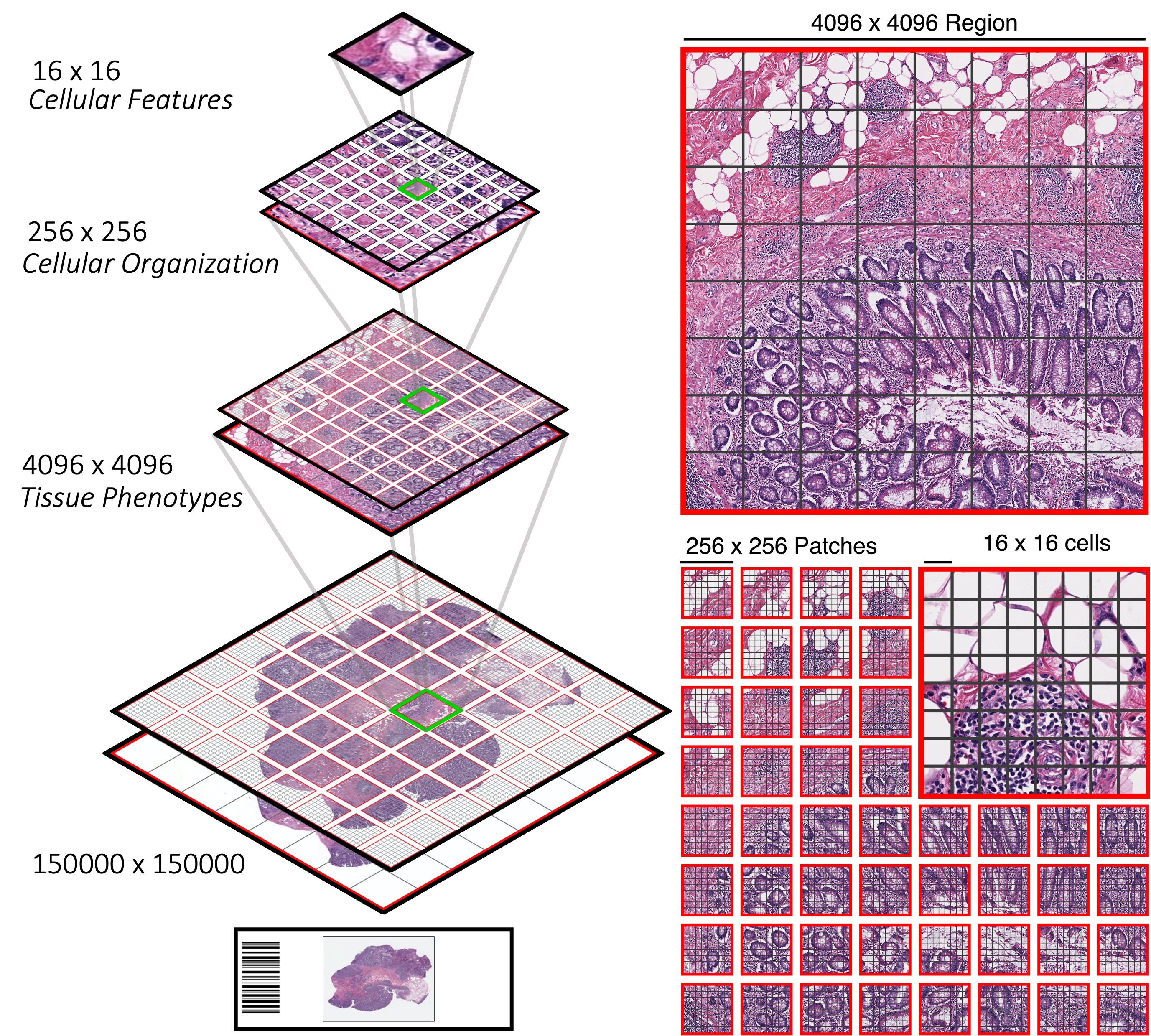
Figure 1: Hierarchical Structure of Whole-Slide Images (WSIs). Left. Unlike natural images, since WSIs have a fixed scale, there exists a hierarchical structure of visual tokens at varying image resolutions. Right. In addition to formulating a single $256\times 256$ image as as sequence of 256 $[16\times 16]$ tokens, we can also view these $256\times 256$ image as being part of a larger, disjoint sequence of $[256\times 256]$ tokens in a $4096\times 4096$ region.

Tissue phenotyping is a fundamental problem in computational pathology (CPATH) that aims at characterizing objective, histopathologic features within gigapixel whole-slide images (WSIs) for cancer diagnosis, prognosis, and the estimation of response-to-treatment in patients [55, 42, 40]. Unlike natural images, whole-slide imaging is a challenging computer vision domain in which image resolutions can be as large as $150000\times 150000$ pixels, with many methods using the following three-stage, weakly-supervised framework based on multiple instance learning (MIL): 1) tissue patching at a single magnification objective (“zoom”), 2) patch-level feature extraction to construct a sequence of embedding instances, and 3) global pooling of instances to construct a slide-level representation for weak-supervision using slide-level labels (e.g. - subtype, grade, stage, survival, origin) [38, 20, 72, 70, 39, 13, 54, 87, 53].

Though achieving “clinical-grade” performance on many cancer subtyping and grading tasks, this three-stage process has a few important design limitations. First, patching and feature extraction are generally fixed to $[256\times 256]$ context regions. Though able to discern fine-grained morphological features such as nuclear atypia or tumor presence, depending on the cancer type, $[256\times 256]$ windows have limited context in capturing coarser-grained features such as tumor invasion, tumor size, lymphocytic infiltrates, and the broader spatial organization of these phenotypes in the tissue microenvironment, as depicted in Figure 1 [7, 23, 16]. Second, in contrast with other image-based sequence modeling approaches such as Vision Transformers (ViTs), MIL uses only global pooling operators due to the large sequence lengths of WSIs [39]. As a result, this limitation precludes the application of Transformer attention for learning long-range dependencies between phenotypes such as tumor-immune localization, an important prognostic feature in survival prediction [65, 45, 1]. Lastly, though recent MIL approaches have adopted self-supervised learning as a strategy for patch-level feature extraction (called tokenization in ViT literature), parameters in the aggregation layers still require training [19, 64, 21, 44, 9, 46, 17]. In viewing patch-based sequence modeling of WSIs in relation to ViTs, we note that the architectural design choice of using Transformer attention enables pretraining of both the tokenization and aggregation layers in ViT models, which is important in preventing MIL models from over- or under-fitting in low-data regimes [24, 47, 14, 6, 34].

To address these issues, we explore the challenge of developing a Vision Transformer for slide-level representation learning in WSIs. In comparison to natural images which are actively explored by ViTs, we note a key difference in modeling WSIs is that visual tokens would always be at a fixed scale for a given magnification objective. For instance, scanning WSIs at a $20\times$ objective results in a fixed scale of approximately $0.5\mu m$ per pixel, allowing for consistent comparison of visual elements that may elucidate important histomorphological features beyond their normal reference ranges. Moreover, WSIs also exhibit a hierarchical structure of visual tokens at varying image resolutions at $20\times$ magnification: the $16\times 16$ images encompass the bounding box of cells and other fine-grained features (stroma, tumor cells, lymphocytes) [23, 37], $256\times 256$ images capture local clusters of cell-to-cell interactions (tumor cellularity) [31, 8, 60, 2], $1024\times 1024$-$4096\times 4096$ images further characterize macro-scale interactions between clusters of cells and their organization in tissue (the extent of tumor-immune localization in describing tumor-infiltrating versus tumor-distal lymphocytes) [1, 10], and finally the overall intra-tumoral heterogeneity of the tissue microenvironment depicted at the slide-level of the WSI [40, 65, 36, 5, 58]. The hypothesis that this work tests is that the judicious use of this hierarchy in self-supervised learning results in better slide-level representations.

We introduce a Transformer-based architecture for hierarchical aggregation of visual tokens and pretraining in gigapixel pathology images, called Hierarchical Image Pyramid Transformer (HIPT). We approach the task of slide-level representation learning in a manner similar to learning long document representations in language modeling, in which we develop a three-stage hierarchical architecture that performs bottom-up aggregation from [$16\times 16$] visual tokens in their respective $256\times 256$ and $4096\times 4096$ windows to eventually form the slide-level representation, as demonstrated in Figure 2 [78, 84]. Our work pushes the boundaries of both Vision Transformers and self-supervised learning in two important ways. By modeling WSIs as a disjoint set of nested sequences, within HIPT: 1) we decompose the problem of learning a good representation of a WSI into hierarchically-related representations each of which can be learned via self-supervised learning, and 2) we use student-teacher knowledge distillation (DINO  [14]) to pretrain each aggregation layers with self-supervised learning on regions as large as $4096\times 4096$.

We apply HIPT to the task of learning representations of gigapixel histopathological images extracted at $20\times$ resolution. We show that our method achieves superior performance to conventional MIL approaches. The difference is pronounced in context-aware tasks such as survival prediction in which larger context is appreciated in characterizing broader prognostic features in the tissue microenvironment [61, 65, 1, 18]. Using K-Nearest Neighbors on the $4096\times 4096$ representations of our model, we outperform several weakly-supervised architectures in slide-level classification – an important step forward in achieving self-supervised slide-level representations. Finally, akin to self-supervised ViTs on natural images that can perform semantic segmentation of the scene layout, we find that the multi-head self-attention in self-supervised ViTs learn visual concepts in histopathology tissue (from fine-grained visual concepts such as cell locations in the $\operatorname{ViT_{256}\textrm{-}16}$ to coarse-grained visual concepts such as broader tumor cellularity in the $\operatorname{ViT_{4096}\textrm{-}256}$), as demonstrated in Figure 3, 4. We make code available at https://github.com/mahmoodlab/HIPT.

2 Related Work

Multiple Instance Learning in WSIs

In general set-based deep learning, Edwards & Storkey and Zaheer et al. proposed the first network architectures operating on set-based data structures, with Brendel et al. demonstrating “bag-of-features” able to reach high accuracy on ImageNet [26, 82, 11]. Concurrently in pathology, Ilse et al. extended set-based network architectures as an approach for multiple instance learning in histology region-of-interests, with Campanella et al. later extending end-to-end weak-supervision on gigapixel WSIs [39, 13]. Lu et al. demonstrated that by using a pretrained ResNet-50 encoder on ImageNet for instance-level feature extraction, only a global pooling operator needs to be trained for weakly-supervised slide-level tasks [54]. Following Lu et al., there have been many variations of MIL that have adapted image pretraining techniques such as VAE-GANs, SimCLR, and MOCO as instance-level feature extraction [86, 46, 64]. Recent variations of MIL have also evolved to extend the aggregation layers and scoring functions [87, 77, 70, 66, 79, 80, 18]. Li et al. proposed a multi-scale MIL approach that performs patching and self-supervised instance learning at $20\times$ and $5\times$ resolution, followed by spatially-resolved alignment of patches[46]. The integration of magnification objectives within WSIs has been followed in other works as well [33, 57, 59, 30], however, we note that combining visual tokens across objectives would not share the same scale. In this work, patching is done at a single magnification objective, with larger patch sizes used to capture macro-scale morphological features, which we hope will contribute towards a shift in rethinking context modeling of WSIs.

Vision Transformers and Image Pyramids

The seminal work of Vaswani et al. has led to remarkable developments in not only language modeling, but also image representation learning via Vision Transformers (ViTs), in which $256\times 256$ images are formulated as an image patch sequence of $[16\times 16]$ visual tokens [73, 24, 71]. Motivated by multiscale, pyramid-based image processing [63, 12, 43], recent progress in ViT architecture development has focused on efficiency and integration of multiscale information (e.g. - Swin, ViL, TNT, PVT, MViT) in addressing the varying scale / aspect ratios of visual tokens [32, 83, 52, 74, 28]. In contrast with pathology, we highlight that learning scale invariance may not be necessary if the image scale is fixed at a given magnification. Similar to our work is NesT and Hierarchical Perciever, which similarly partitions and then aggregates features from non-overlapping image regions via Transformer blocks[85, 15]. A key difference is that we show ViT blocks at each stage can be separately pretrained for high-resolution encoding (up to $4096\times 4096)$.

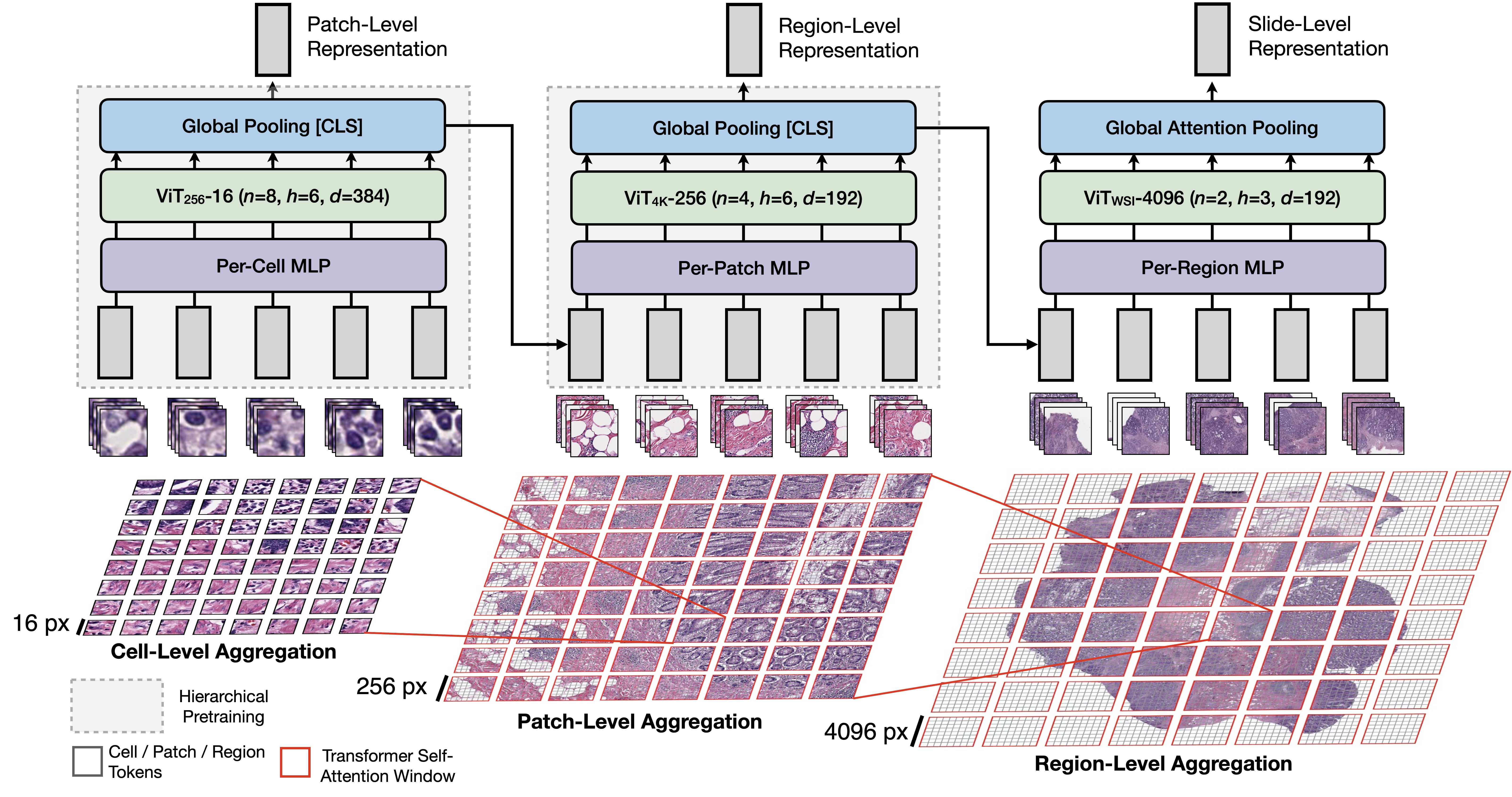
Figure 2: HIPT Architecture. Motivated by the use of hierarchical representations in natural language processing, where embeddings can be aggregated at the character-, word-, sentence- and paragraph-level to form document representations, we aggregate visual tokens at the $\textbf{x}_{16}$ cell-, $\textbf{x}_{256}$ patch-, $\textbf{x}_{4096}$ region-level to form slide representations. To also model important dependencies between visual concepts at each stage, we adapt Transformer self-attention as a permutation-equivariant aggregation layer. Note that since the complexity of patching $\textbf{x}_{4096}$ regions with $\textbf{x}_{256}$ tokens is the same as patching $\textbf{x}_{256}$ images with $\textbf{x}_{16}$ tokens, we can pretrain aggregation layers for high-resolution images using similar self-supervised ViT techniques for low-resolution images.

3 Method

3.1 Problem Formulation

Patch Size and Visual Token Notation: We use the following notation to distinguish between the sizes of “images” and “tokens” that correspond to that image. For an image x with resolution $L\times L$ (or $\textbf{x}_{L}$), we refer to sequence of extracted visual tokens from non-overlapping patches (of size $[l\times l]$) within $\textbf{x}_{L}$ as $\{\textbf{x}_{l}^{(i)}\}_{i=1}^{M}\in\mathbb{R}^{M\times d_{l}}$, where $M$ is the sequence length and $d$ is the embedding dimension extracted for $l$-sized tokens. In working with multiple image resolutions (and their respective tokens) in a WSI, we additionally denote the shape of visual tokens (and the patching parameter) within $\textbf{x}_{L}$ image as $[l\times l]$ (using brackets). For natural images with size $\textbf{x}_{256}$, ViTs generally use $l=L^{1/2}=16$ which results in a sequence length of $M=256$. Additionally, we denote a ViT working on a $L$-sized image resolution with $[l\times l]$ tokens as $\operatorname{ViT}_{L}-l$. For $\textbf{x}_{\text{WSI}}$ (referring to the slide-level resolution of the WSI), MIL approaches choose $l=256$ which fits the input shape of CNN encoders that can be pretrained and using for tokenization, resulting in $M>10,000$ (variable due to the total area of segmented tissue content).

Slide-Level Weak Supervision: For a WSI $\textbf{x}_{\text{WSI}}$ with outcome $y$, the goal is to solve the slide-level classification task $P(y|\textbf{x}_{\text{WSI}})$. Conventional approaches for solving this task use a three-stage MIL framework which performs: 1) $[256\times 256]$-patching, 2) tokenization, and 3) global attention pooling. $\textbf{x}_{\text{WSI}}$ is formulated as the sequence $\{\textbf{x}_{256}^{(i)}\}_{i=1}^{M}\in\mathbb{R}^{M\times 1024}$ which results from using a ResNet-50 encoder pretrained on ImageNet (truncated after the 3rd residual block). Due to the large sequence lengths with $l=256$, neural network architectures in this task are limited to per-patch and global pooling operators in extracting a slide-level embedding for downstream tasks.

3.2 Hierarchical Image Pyramid Transformer (HIPT) Architecture

In adapting ViTs for slide-level representation learning, we reiterate two important challenges distinct from computer vision in natural images: 1) the fixed scale of visual tokens and their hierarchical relationships across image resolutions, and 2) the large sequence lengths of unrolled WSIs. As mentioned, visual tokens in histopathology are generally object-centric (and vary in granularity) across image resolutions, and also have important contextual dependencies such as tumor-immune (inferring favorable prognosis) or tumor-stroma interactions (inferring invasion). Patching with small visual tokens at high objectives ($\textbf{x}_{256}$ at $20\times$) results in large sequence lengths that make self-attention intractable, whereas patching with large visual tokens at low objectives results in loss-of-detail of fine-grained morphological structures ($\textbf{x}_{256}$ at $5\times$) that still requires $[256\times 256]$ patching at $20\times$.

To capture this hierarchical structure and the important dependencies that may exist at each image resolution, we approach WSIs similar to long documents as a nested aggregation of visual tokens that recursively break down into smaller tokens until the cell-level (Figure 2), written as:

$$\operatorname{HIPT}(\mathbf{x}_{\text{WSI}})=\operatorname{ViT_{WSI}\textrm{-}4096}\big{(}\big{\{}\operatorname{CLS}_{4096}^{(k)}\big{\}}_{k=1}^{M}\big{)}$$

$$\rightarrow\operatorname{CLS}_{4096}^{(k)}=\operatorname{ViT_{4096}\textrm{-}256}\big{(}\{\operatorname{CLS}_{256}^{(j)}\}_{i=1}^{256}\big{)}$$

$$\rightarrow\operatorname{CLS}_{256}^{(j)}=\operatorname{ViT_{256}\textrm{-}16}\big{(}\{\textbf{x}_{16}^{(i)}\}_{i=1}^{256}\big{)}$$

where 256 is the sequence length of $[16\times 16]$- and $[256\times 256]$-patching in $\textbf{x}_{256}$ and $\textbf{x}_{4096}$ images respectively, and $M$ is the total number of $\textbf{x}_{4096}$ images in $\textbf{x}_{\text{WSI}}$. For ease of notation, we refer to $\textbf{x}_{16}$ images as being at the cell-level, $\textbf{x}_{256}$ images as being at the patch-level, $\textbf{x}_{4096}$ images as being at the region-level, with the overall WSI being the slide-level. In choosing these image sizes, the input sequence length of tokens is always $M=256$ in the forward passes for the $\operatorname{ViT_{256}\textrm{-}16}$ and $\operatorname{ViT_{4096}\textrm{-}256}$ (cell- and patch-level aggregation), and usually $M<256$ in the forward pass for the $\operatorname{ViT_{\text{WSI}}\textrm{-}4096}$ (slide-level aggregation). The [CLS] tokens from $\operatorname{ViT_{256}\textrm{-}16}$ (the output of the model) are used as the input sequence for $\operatorname{ViT_{4096}\textrm{-}256}$, with the [CLS] tokens from $\operatorname{ViT_{4096}\textrm{-}256}$ subsequently used as the input sequence for $\operatorname{ViT_{\text{WSI}}\textrm{-}4096}$, with the number of total visual tokens at each stage decreasing geometrically by a factor of 256. In choosing small ViT backbones for each stage, HIPT has less than 10M parameters and is easy-to-implement and train on commercial workstations. We describe each stage below.

ViT${}_{\textbf{256}}$-16 for Cell-Level Aggregation

The computation of $\mathbf{x}_{16}$ cell-level token aggregation within $\mathbf{x}_{256}$ windows follows implementing the vanilla ViT in natural images[24]. Given a $\mathbf{x}_{256}$ patch, the ViT unrolls this image as a sequence of non-overlapping $[16\times 16]$ tokens followed by a linear embedding layer with added position embeddings to produce a set of 384-dim embeddings $\{\textbf{x}_{16}^{(i)}\}_{i=1}^{256}\in\mathbb{R}^{256\times 384}$, with a learnable [CLS] token added to aggregate cell embeddings across the sequence. We choose $l=16$ in this setting to not only follow conventional ViT architectures, but also model important inductive biases in histopathology as at this resolution, a $[16\times 16]$ bounding box at $20\times\approx 8\mu m^{2}$ area encodes visual concepts that are object-centric in featurizing single cells (e.g. - cell identity, shape, roundness).

ViT${}_{\textbf{4096}}$-256 for Patch-Level Aggregation

To represent $\mathbf{x}_{4096}$ regions, despite the image resolution being much larger than conventional natural images, the number of tokens remains the same since the patch size scales with the image resolution. From the previous stage, we use $\operatorname{ViT_{256}\textrm{-}16}$ to tokenize non-overlapping $\mathbf{x}_{256}$ patches within each $\mathbf{x}_{4096}$ region, forming the sequence $\{\operatorname{[CLS]}_{256}^{(j)}\}_{j=1}^{256}$ that can be plugged into a ViT block to model larger image contexts. We use a $\operatorname{ViT_{4096}\textrm{-}256(n=4,h=3,d=192)}$ with output $\operatorname{[CLS]}_{4096}$.

ViT${}_{\textbf{WSI}}$-4096 for Region-Level Aggregation

In computing the slide-level representation for $\textbf{x}_{\text{WSI}}$, we use a $\operatorname{ViT_{\text{WSI}}\textrm{-}4096(n=2,h=3,d=192)}$ in aggregating the $\operatorname{[CLS]}_{4096}$ tokens. $M$ ranges from $1-256$ in our observations depending on size of the WSI. Due to potential tissue segmentation irregularities in patching at $[4096\times 4096]$, we ignore positional embeddings at this stage.

	BRCA Subtyping		NSCLC Subtyping		RCC Subtyping
Architecture	25% Training	100% Training	25% Training	100% Training	25% Training	100% Training
MIL [54]	0.673 $\pm$ 0.112	0.778 $\pm$ 0.091	0.857 $\pm$ 0.059	0.892 $\pm$ 0.042	0.904 $\pm$ 0.055	0.959 $\pm$ 0.015
CLAM-SB [54]	0.796 $\pm$ 0.063	0.858 $\pm$ 0.067	0.852 $\pm$ 0.034	0.928 $\pm$ 0.021	0.957 $\pm$ 0.012	0.973 $\pm$ 0.017
DeepAttnMISL [80]	0.685 $\pm$ 0.110	0.784 $\pm$ 0.061	0.663 $\pm$ 0.077	0.778 $\pm$ 0.045	0.904 $\pm$ 0.024	0.943 $\pm$ 0.016
GCN-MIL [86]	0.727 $\pm$ 0.076	0.840 $\pm$ 0.073	0.748 $\pm$ 0.050	0.831 $\pm$ 0.034	0.923 $\pm$ 0.012	0.957 $\pm$ 0.012
DS-MIL [46]	0.760 $\pm$ 0.088	0.838 $\pm$ 0.074	0.787 $\pm$ 0.073	0.920 $\pm$ 0.024	0.949 $\pm$ 0.028	0.971 $\pm$ 0.016
HIPT	0.821 $\pm$ 0.069	0.874 $\pm$ 0.060	0.923 $\pm$ 0.020	0.952 $\pm$ 0.021	0.974 $\pm$ 0.012	0.980 $\pm$ 0.013
$\text{ResNet-50}_{\text{IN}}$ (Mean)	0.638 $\pm$ 0.089	0.667 $\pm$ 0.070	0.696 $\pm$ 0.055	0.794 $\pm$ 0.035	0.862 $\pm$ 0.030	0.951 $\pm$ 0.016
$\operatorname{ViT_{256}-16}$ (Mean)	0.605 $\pm$ 0.092	0.725 $\pm$ 0.083	0.622 $\pm$ 0.067	0.742 $\pm$ 0.045	0.848 $\pm$ 0.032	0.899 $\pm$ 0.027
$\operatorname{ViT_{4096}-256}$ (Mean)	0.682 $\pm$ 0.055	0.775 $\pm$ 0.042	0.773 $\pm$ 0.048	0.889 $\pm$ 0.027	0.916 $\pm$ 0.022	0.974 $\pm$ 0.016

Table 1: Slide-Level Classification. Top Row. Ablation study assessing 10-fold cross-validated AUC performance of HIPT across other weakly-supervised architectures. For RCC subtyping, we report the macro-averaged AUC performance across the three subtypes. Bottom Row. Ablation study assessing K-Nearest Neighbors (KNN) performance using the average pre-extracted embeddings.

3.3 Hierarchical Pretraining

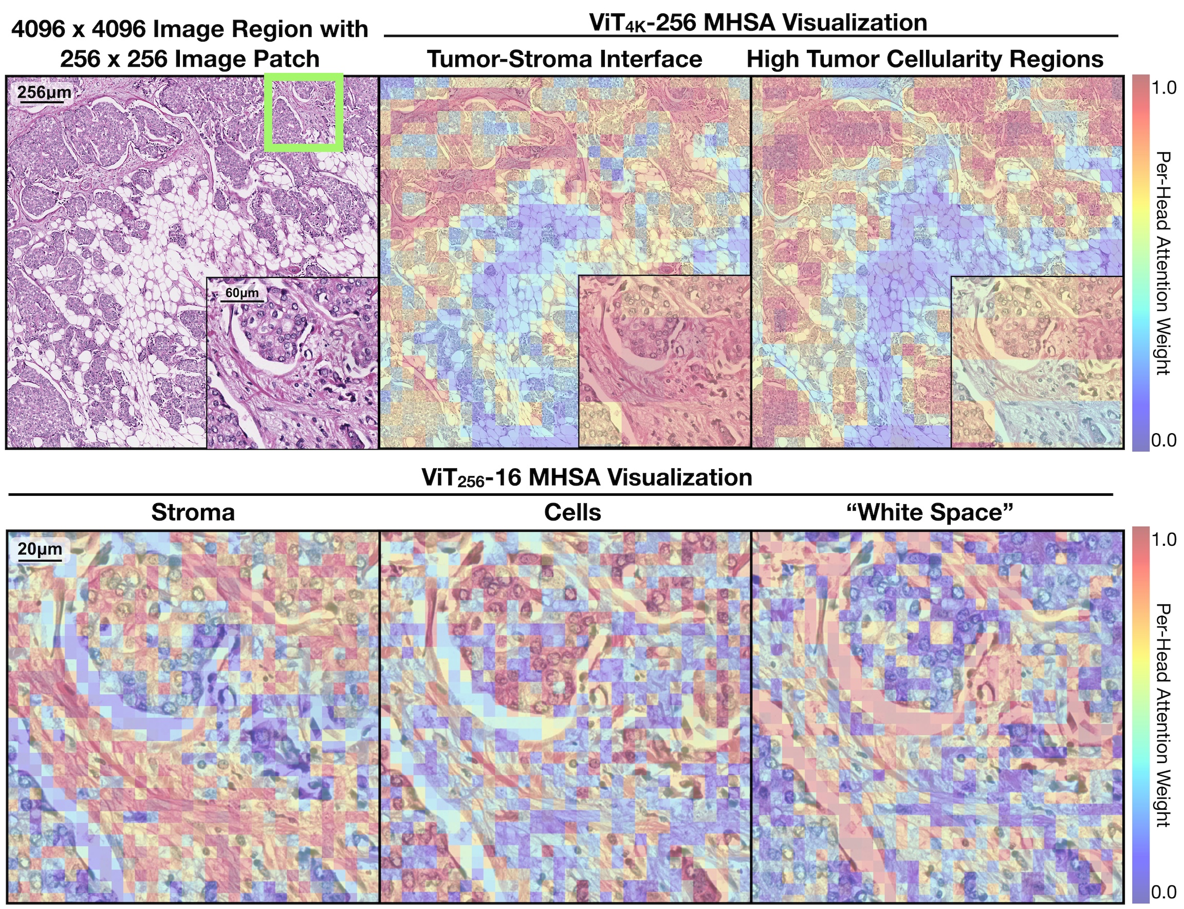
Figure 3: Multi-Head Self-Attention Visualization of Self-Supervised ViTs. For Invasive Ductal Carcinoma (IDC), We show self-supervised visualizations for $\operatorname{ViT_{256}\textrm{-}16}$ and $\operatorname{ViT_{4096}\textrm{-}256}$, pretrained on $\textbf{x}_{256}$ and $\textbf{x}_{4096}$ regions respectively. For $\textbf{x}_{256}$ patches, $\operatorname{ViT_{256}\textrm{-}16}$ is able to delineate stroma, cell, and ”white space” presence in $\textbf{x}_{16}$ tokens. For $\textbf{x}_{4096}$ regions, $\operatorname{ViT_{4096}\textrm{-}256}$ delineates coarse-grained morphological features such as tumor nests and their surrounding desmoplastic (loose) stroma.

In building a MIL framework using only Transformer blocks, we additionally explore and pose a new challenge referred to as slide-level self-supervised learning - which aims at extracting slide-level feature representations in gigapixel images for downstream diagnostic and prognostic tasks. This is an important problem as current slide-level training datasets in CPATH typically have between 100 to 10,000 data points, which may cause MIL methods to overfit due to over-parameterization and lack of labels. To address this problem, we hypothesize that the recursive nature of HIPT in using Transformer blocks for image representation learning can enable conventional ViT pretraining techniques (such as DINO [14]) to generalize across stages (of similar subproblems) for high-resolution images. To pretrain HIPT, first, we leverage DINO to pretrain $\operatorname{ViT_{256}\textrm{-}16}$. Then, keeping fixed the weights of $\operatorname{ViT_{256}\textrm{-}16}$, we re-use $\operatorname{ViT_{256}\textrm{-}16}$ as the embedding layer for $\operatorname{ViT_{4096}\textrm{-}256}$ in a second stage of DINO. We refer to this procedure as hierarchical pretraining, which is similarly performed in the context of learning deep belief networks [27] and hierarchical transformers for long documents[84]. Though hierarchical pretraining does not reach the slide-level, we show that: 1) pretrained $\textbf{x}_{4096}$ representations in self-supervised evaluation are competitive with supervised methods for slide-level subtyping, and that 2) HIPT with two-stage hiearchical pretraining can reach state-of-the-art performance.

Stage 1: 256 $\times$ 256 Patch-Level Pretraining

To pretrain $\operatorname{ViT_{256}\textrm{-}16}$, we use the the DINO framework for pretraining of $\mathbf{x}_{256}$ patches, in which a student network $\phi_{s_{256}}$ is trained to match the probability distribution of a siamese teacher network $\phi_{t_{256}}$ using a cross-entropy loss $-p_{t_{256}}(\cdot)\operatorname{log}p_{s_{256}}(\cdot)$ with momentum encoding, with $p_{t_{256}},p_{s_{256}}$ denoting the outputs of $\phi_{t_{256}}(\cdot),\phi_{s_{256}}(\cdot)$ respectively for $\mathbf{\mathbf{x}}_{256}$. As data augmentation for each $\mathbf{x}_{256}$ patch, DINO constructs a set of $M_{l}=8$ local views ($\mathbf{x}_{96}$ crops, passed through $\phi_{s_{256}}$) and $M_{g}=2$ global views ($\mathbf{x}_{224}$ crops, passed through $\phi_{t_{256}}$) to encourage local-to-global correspondences between the student and teacher, minimizing the function:

$$\min_{\theta_{s_{256}}}\sum_{\left\{\mathbf{x}_{224}^{(i)}\right\}_{i=1}^{M_{g}}}^{M_{g}=2}\sum_{\left\{\mathbf{x}_{96}^{(j)}\right\}_{j=1}^{M_{l}}}^{M_{l}=8}H\Big{(}p_{t_{256}}(\mathbf{x}_{224}^{(i)}),p_{s_{256}}\left(\mathbf{x}_{96}^{(j)}\right)\Big{)}$$

An intriguing property that makes this data augmentation suitable for histology data is again the natural part-whole hierarchy of cells in a tissue patch. In comparison to natural images in which $[96\times 96]$ crops may capture only colors and textures without any semantic information, at $20\times$, local $[96\times 96]$ crops would capture the context of multiple cells and their surrounding extracellular matrices, which has shared mutual information with the broader cellular communities. Similar to the original DINO implementation, we use horizontal flips and color jittering for all views, with solarizing performed on one of the global views.

Stage 2: 4096 $\times$ 4096 Region-Level Pretraining

With the sequence lengths and computational complexity in tokenizing $\mathbf{x}_{4096}$ regions similar to that of $\mathbf{x}_{256}$ patches, we can also borrow an almost identical DINO recipe in also pretraining $\operatorname{ViT_{4096}\textrm{-}256}$ and defining student-teacher networks $\phi_{s_{4096}}(\cdot),\phi_{t_{4096}}(\cdot)$ at this stage. Following extracting $\operatorname{[CLS]}_{256}$ tokens from $\operatorname{ViT_{256}\textrm{-}16}$ as input for $\operatorname{ViT_{4096}\textrm{-}256}$ input, we rearrange $\{\operatorname{[CLS]}_{256}^{(j)}\}_{j=1}^{M=256}$ as a $16\times 16\times 384$ 2D feature grid for data augmentations, performing $[6\times 6],[14\times 14]$ local-global crops in matching the scale of $[96\times 96],[224\times 224]$ crops for $256\times 256$ inputs. As additional data augmentation, We apply standard dropout ($p=0.10$) to all views following work in Gao et al. [29].

4 Experiments

Pretraining:

We pretrain $\operatorname{ViT_{256}\textrm{-}16}$ and $\operatorname{ViT_{4096}\textrm{-}256}$ in different stages, using 10,678 FFPE (formalin-fixed, paraffin-embedded) H&E-stained diagnostic slides from 33 cancer types in the The Genome Cancer Atlas (TCGA), and extracted 408,218 $\textbf{x}_{4096}$ regions at an $20\times$ objective ($M\approx 38$ regions per slide) for pretraining $\operatorname{ViT_{4096}\textrm{-}256}$, with a total of 104M $\textbf{x}_{256}$ patches for pretraining $\operatorname{ViT_{256}\textrm{-}16}$ [51]. For $\operatorname{ViT_{256}\textrm{-}16}$, we trained for 400,000 iterations using the AdamW optimizer with a batch size of $256$, base learning rate of 0.0005, with the first 10 epochs used to warm up to the base learning rate followed by decay using a cosine schedule. A similar implementation was used for $\operatorname{ViT_{4096}\textrm{-}256}$, with the model trained for 200,000 iterations using the pre-extracted $\operatorname{[CLS}]$ tokens from $\operatorname{ViT_{256}\textrm{-}16}$.

Fine-tuning:

Following hierarchical pretraining, we use the pretrained weights to initialize (and freeze) the $\operatorname{ViT_{256}\textrm{-}16}$ and $\operatorname{ViT_{4096}\textrm{-}256}$ subnetworks, with only a lightweight $\operatorname{ViT_{\text{WSI}}\textrm{-}4096}$ finetuned. Our work can be viewed as a formulation of MIL that pretrains not only the $[256\times 256]$ instance-level feature extraction step, but also the downstream aggregation layers which extract coarse-grained morphological features. We finetuned HIPT (and its comparisons) for 20 epochs using the Adam optimizer, batch size of $1$ with $32$ gradient accumulation steps, and a learning rate of $0.01$. For survival prediction, we used the survival cross-entropy loss by Zadeh & Schmidt[81].

Tasks & Comparisons:

We experiment on several slide-level classification and survival outcome prediction tasks across different organ types in the TCGA [51]. In comparisons with state-of-the-art weakly-supervised architectures, we tested Attention-Based MIL (ABMIL), and it’s variants that use clustering losses (CLAM-SB), clustering prototypes (DeepAttnMISL), modified scoring & pooling functions (DS-MIL), and graph message passing (GCN-MIL), which used the same hyperparameters as HIPT. Since these methods are agnostic of input features, all comparisons used the pretrained $\operatorname{ViT_{256}\textrm{-}16}$ as instance-level feature extraction. In addition, we also compared variations of HIPT without pretraining and self-attention. Finally, we qualitatively study the attention maps that hierarchical self-supervised ViTs learn in computational histopathology.

Architecture	IDC	CRC	CCRCC	PRCC	LUAD	STAD
ABMIL [39]	0.487 $\pm$ 0.079	0.566 $\pm$ 0.075	0.561 $\pm$ 0.074	0.671 $\pm$ 0.076	0.584 $\pm$ 0.054	0.562 $\pm$ 0.049
DeepAttnMISL [80]	0.472 $\pm$ 0.023	0.561 $\pm$ 0.088	0.521 $\pm$ 0.084	0.472 $\pm$ 0.162	0.563 $\pm$ 0.037	0.563 $\pm$ 0.067
GCN-MIL [50, 86]	0.534 $\pm$ 0.060	0.538 $\pm$ 0.049	0.591 $\pm$ 0.093	0.636 $\pm$ 0.066	0.592 $\pm$ 0.070	0.513 $\pm$ 0.069
DS-MIL [46]	0.472 $\pm$ 0.020	0.470 $\pm$ 0.053	0.548 $\pm$ 0.057	0.654 $\pm$ 0.134	0.537 $\pm$ 0.061	0.546 $\pm$ 0.047
HIPT	0.634 $\pm$ 0.050	0.608 $\pm$ 0.088	0.642 $\pm$ 0.028	0.670 $\pm$ 0.065	0.538 $\pm$ 0.044	0.570 $\pm$ 0.081

Table 2: Survival Prediction. Ablation study assessing cross-validated c-Index of HIPT across other weakly-supervised architectures.

4.1 Slide-Level Classification

Dataset Description

We follow the study design in  [54]; we examined the following tasks evaluated using a 10-fold cross-validated AUC: 1) Invasive Ductal (IDC) versus Invasive Lobular Carcinoma (ILC) in Invasive Breast Carcinoma (BRCA) subtyping, 2) Lung Adenocarcinoma (LUAD) versus Lung Squamous Cell Carcinoma (LUSC) in Non-Small Cell Lung Carcinoma (NSCLC) subtyping, and 3) Clear Cell, Papillary, and Chromophobe Renal Cell Carcinoma (CCRCC vs. PRCC vs. CHRCC) subtyping, with all methods finetuned (for 20 epochs) with varying percentange folds of training data (100% / 25%) as data efficiency experiments. Despite RCC subtyping being a relative easy slide-level task due to having distinct subtypes, we ultimately include this task as a benchmark for self-supervised comparisons.

Weakly-Supervised Comparison

Classification results are summarized in Table 1. Overall, across all tasks and different percentage folds, HIPT consistently achieves the highest macro-averaged AUC performance across all tasks. In comparison with the best performing baseline, CLAM-SB, HIPT achieves a performance increase of 1.86%, 2.59%, 0.72% on BRCA, NSCLC and RCC subtyping respectively using 100% of training data, with the margin in performance increase widening to 3.14%, 8.33%, 1.78% respectively using 25% of training data. Similar performance increases are demonstrated on other tasks. HIPT demonstrates the most robust performance when limiting training data, with AUC decreasing slightly from $0.980$ to $0.974$.

K-Nearest Neighbor (KNN)

We take the mean embedding of the pre-extracted embeddings, followed by a KNN evaluation for the above tasks. As a baseline, we use a ResNet-50 pretrained on ImageNet to extract patch-level embeddings. We compare with pre-extracted $\operatorname{ViT_{256}\textrm{-}16}$ patch embeddings from DINO pretraining, and pre-extracted $\operatorname{ViT_{4096}\textrm{-}256}$ region-level embeddings from hierarchical pretraining, with results summarized also in Table 1. In using the average embedding of each WSI as the “slide-level representation”, we find that $\operatorname{ViT_{4096}\textrm{-}256}$ region-level embeddings in HIPT outperform patch-level embeddings across all tasks, which can be attributed to the broader image contexts used in the WSI for pretraining, and can be intuitively viewed as a closer proxy to the slide-level view than small patches. $\operatorname{ViT_{4096}\textrm{-}256}$ region-level embeddings surpass the AUC performance of weakly-supervised approaches in BRCA and RCC subtyping using 100% of training data.

4.2 Survival Prediction

Dataset Description

For survival outcome prediction, we validated on the IDC, CCRCC, PRCC, and LUAD cancer types which have relatively large sample sizes in the TCGA, in addition to Colon & Rectal (CRC) and Stomach Adenocarcinoma (STAD) which have been frequently evaluated in real-world clinical studies due to their substantial human intra-observer variability [25, 75, 68]. All tasks were evaluated using cross-validated concordance index (c-Index).

Weakly-Supervised Comparison

For the following survival prediction tasks in which learning context-aware relationships are important, we observe much larger increases in performance, summarized in Table 2. Overall, HIPT achieves the best c-Index performance in the IDC, COADREAD, CCRCC, and STAD cancer types, with the largest improvement demonstrated in IDC (0.634) and COADREAD (0.608) in comparison to other methods. Though other methods such as GCN-MIL use message passing for learning context-aware features, we note that the number of layers needed to achieve similar image receptive fields may cause the number of neighbors to grow exponentially [48]. In modeling important long-range dependencies between instances using self-attention across various stages of the hierarchy, the Transformer attention in HIPT is able to capture regional perturbations that have been well characterized as portending worse outcome across different cancer types, as further visualized in Figure  3, 4 [1, 76, 75, 68].

4.3 Self-Supervised ViTs Find Unique Morphological Phenotypes

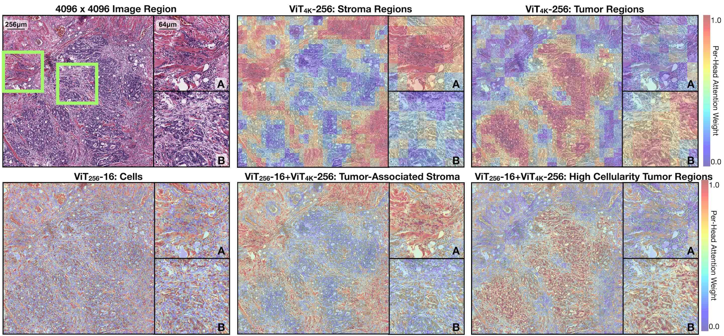
Figure 4: Hierarchical Attention Maps in HIPT. For Colorectal Cancer (CRC), we observe similar delineation of stroma, cells, and ”white space” presence in $\operatorname{ViT_{256}\textrm{-}16}$, and localizing tumor invasion into stroma and muscle (A) and poorly-differentiated glands (B) from $\operatorname{ViT_{4096}\textrm{-}256}$. In factorizing these attention distributions together, we develop hierarchical attention visualizations which can visualize tumor cells with associated stromal tissue and high tumor cellularity regions containing poorly-differentiated glands.

ViT${}_{\textbf{256}}$-16 Attention Maps. For $\mathbf{x}_{256}$ patches, we visualize the different attention heads in MHSA and reveal that ViTs in pathology are able to isolate distinct morphological features. From visual assessment by a board-certified pathologist across several different cancer types, we observe that MHSA in $\operatorname{ViT_{256}\textrm{-}16(n=8,h=6,d=384)}$ captures three distinct fine-grained morphological phenotypes as illustrated in Figure 3, with general stroma tissue and red blood cells attended in $h=1,2$, cells (normal, atypical, lymphocyte) attended in $h=3,4$, and “white spaces” (luminal spaces, fat regions, air pockets) attended in $h=5,6$. This observation is in line with current studies that have introspected self-supervised ViT models, in which the attention heads can be used as a method for object localization or discovery [14, 67]. In the application to histopathology tissue, our introspection reveals that the visual tokens at the $[16\times 16]$ cell-level directly corroborate with semantic, object-centric structures at the $20\times$ objective.

ViT${}_{\textbf{4096}}$-256 Attention Maps. For $\mathbf{x}_{4096}$ regions, we further visualize the attention heads in MHSA from our pretrained $\operatorname{ViT_{4096}\textrm{-}256(n=4,h=6,d=192)}$ model, capturing two distinct coarse-grained phenotypes: tumor-stroma interface attended in $h=1,2,3$, and nested tumor cells and other high tumor cellularity regions in $h=4,5,6$. In comparison with the $\operatorname{ViT_{256}\textrm{-}16}$ attention maps which may capture only nuclear features (e.g. - nuclear atypia, shape and size of cells), $\operatorname{ViT_{4096}\textrm{-}256}$ attention maps are able to model the patterns of nested tumor growth, tumor invasion into fat and stroma regions, and other tissue-to-tissue relationships (Figure  3). In factorizing the attention distribution of $[16\times 16$] cells from $\operatorname{ViT_{256}\textrm{-}16}$ onto highly-attended $[256\times 256]$ patches from $\operatorname{ViT_{4096}\textrm{-}256}$, we can create a hierarchical attention map, which is able to distinguish tumor cells in stroma tissue from tumor cells in dense tumor cellularity regions (Figure  4). Overall, these captured coarse- and fine-grained morphological features corroborate with the observed performance increases in both finetuning HIPT in weakly-supervised learning and using averaged HIPT features in KNN evaluation. Additional visualizations are found in the Supplement.

4.4 Further Ablation Experiments

Additional experiments are included in the Supplementary Materials, with main findings highlighted below:
The role of pretraining. Hierarchical pretraining of $\operatorname{ViT_{4096}\textrm{-}256}$ is an important component in our method, as HIPT variants without pretraining overfit in MIL tasks.
Comparing patch-level representations. We assessed quality of other embedding types, and found that $\operatorname{ViT_{256}\textrm{-}16}$ achieves strong representation quality of image patches.
Organ-specific versus pan-cancer pretraining. We additionally assessed the performance of $\operatorname{ViT_{256}\textrm{-}16}$ pretraining on different data distributions, with improved performance in cell localization with pan-cancer pretraining.

5 Conclusion

We believe our work is an important step towards self-supervised slide-level representation learning, demonstrating pretrained and finetuned HIPT features achieve superior performance on weakly-supervised and KNN evaluation respectively. Though DINO was used for hierarchical pretraining with conventional ViT blocks, we hope to explore other pretraining methods such as mask patch prediction[24, 6] and efficient ViT architectures[83, 52, 74, 47].

Limitations: A limitation of HIPT is the difficulty in pretraining the last aggregation layer due to the small number of WSI data points. In addition, end-to-end hierarchical pretraining of HIPT is computationally intractable on commercial workstations, with pretraining needed to be performed in stages. Lastly, the study design of this work has several constraints, such as: 1) excluded slides in each TCGA cohort due to limited tissue content and difficulty patching at $[4096\times 4096]$, 2) $\operatorname{ViT_{256}\textrm{-}16}$ pretraining performed on almost all of TCGA and evaluation lacking independent test cohorts, 3), analysis limited to TCGA, which overrepresents patients with European ancestry and not representative of the rich genetic diversity in the world[69].

Broader Impacts: Many problems in biology and medicine have hierarchical-like relationships[56, 49, 35]. For instances, DNA motifs within exon sequences which contributes towards protein structure, gene expression, and genetic traits[4, 41, 22]. Our idea of pretraining neural networks based on hierarchical relationships in large, heterogeneous data modalities to derive a patient- or population-level representation can be extended to other domains.

6 Acknowledgements

We thank Felix Yu, Ming Y. Lu, Chunyuan Li, and the BioML group at Microsoft Research New England for their feedback. This work was supported in part by the BWH president’s fund, BWH & MGH Pathology, Google Cloud Research Award, and NIGMS R35GM138216 (F.M.). R.J.C. was also supported by the NSF Graduate Fellowship. T.Y.C. was also supported by the NIH T32CA251062. R.G.K. gratefully acknowledges funding from CIFAR.

Supplementary Material

Appendix A Multi-Head Self-Attention

We briefly introduce self-attention then extend it to the multi-head version. Recall that $\{\textbf{x}_{l}^{(i)}\}_{i=1}^{M}\in\mathbb{R}^{M\times d_{l}}$ denotes the sequence of visual token extracted from a $L\times L$ patch, where $M$ is the sequence length and $d_{l}$ is the embedding dimension extracted for $l$-sized tokens. For simplicity, we ignore the the subscript $l$ and lower the superscript $i$ to the subscript. The sequence of visual token is re-written as $S=\{\textbf{x}_{i}\}_{i=1}^{M}\in\mathbb{R}^{M\times d_{l}}$

To perform self-attention, we add three matrices $\boldsymbol{W}_{q}$,$\boldsymbol{W}_{k}$ and $\boldsymbol{W}_{v}$ $\in\mathbb{R}^{d_{l}\times d_{l}}$ used to compute the relationship between the token itself $\textbf{x}_{i}$ and other tokens $\textbf{x}_{j}$ in $S$. Specifically,

$$\boldsymbol{q}_{i}=\boldsymbol{W}_{q}\textbf{x}_{i},\boldsymbol{k}_{i} =\boldsymbol{W}_{k}\textbf{x}_{i},\boldsymbol{v}_{i}=\boldsymbol{W}_{v}\textbf{x}_{i}$$

$$w_{ij} =\textrm{softmax}(\frac{\boldsymbol{q}_{i}^{\intercal}\boldsymbol{k}_{j}}{\sqrt{d}_{l}})$$

$$\boldsymbol{o}_{i} =\sum_{j}w_{ij}\boldsymbol{v}_{j},$$

where $\boldsymbol{q}_{i}$, $\boldsymbol{k}_{i}$ and $\boldsymbol{v}_{i}$ are query, key and value vector of input token $\textbf{x}_{i}$. Intuitively, each visual token $\textbf{x}_{i}$ computes a similarity score with other tokens and use the normalized similarity score to perform weighted-sum of value vectors of other tokens. The query, key and value vector space are captured by $\boldsymbol{W}_{q}$,$\boldsymbol{W}_{k}$ and $\boldsymbol{W}_{v}$ learned from data. To increase the feature expressiveness, we increase the number of matrices from 1 to $h$ which leads to a set of matrices $\{\boldsymbol{W}^{h^{\prime}}_{q},\boldsymbol{W}^{h^{\prime}}_{k},\boldsymbol{W}^{h^{\prime}}_{v}|h^{\prime}=1,2,3,\dots,h\}$ for the input sequence. The self-attention with $h>1$ is called multi-head self-attention (MHSA), which we use not only as the building block in permutation-equivariant aggregation of visual tokens, but also demonstrate to learn representations of morphological phenotypes, as seen in Figure 5.

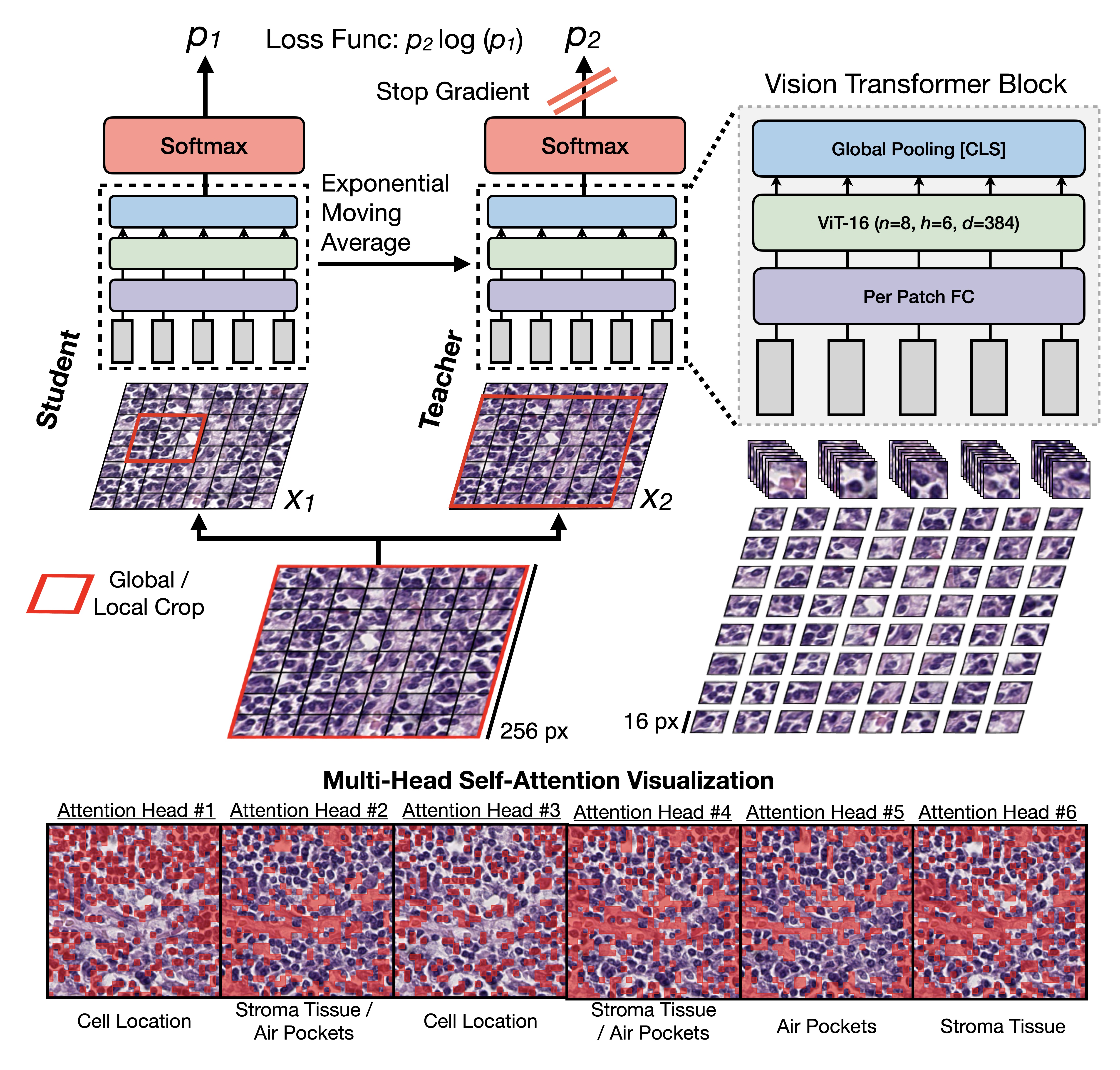
Figure 5: $\operatorname{\mathbf{ViT_{256}\textrm{-}16}}$ DINO Pretraining. Self-supervision using knowledge distillation in DINO to pretrain $\operatorname{ViT_{256}\textrm{-}16}$ on histology image patches [14]. A student network $\phi_{s_{\text{256}}}$ is trained to match the probability distribution of a Siamese teacher network $\phi_{t_{\text{256}}}$ using a cross-entropy loss, with $\phi$ parameterized using a $\operatorname{ViT_{256}\textrm{-}16}$ model, and local and global crops applied as data augmentation. Interpretability of multi-head attention weights reveal that DINO learns distinct morphological phenotypes. In ”red” are high-attention visual tokens with attention weights greater than 0.5.

Appendix B Additional Implementation Details

Efficient Inference and Batching in HIPT

At inference time, we feed in $\textbf{x}_{\text{WSI}}\in\mathbb{R}^{M\times 256\times 256\times[3\times 16\times 16]}$ with a slide-level batch size $B_{\text{WSI}}=1$ into HIPT, in which the respective dimensions correspond to: length of $\mathbf{x}_{4096}$ regions in $\textbf{x}_{\text{WSI}}$, length of $\mathbf{x}_{256}$ patches in $\mathbf{x}_{4096}$, length of $\mathbf{x}_{16}$ cells in $\mathbf{x}_{256}$, and the remaining dimensions being the $\mathbf{x}_{16}$ shape. Without pre-extracting any tokens, inference can be performed in first defining a $\operatorname{DataLoader}$ class over a $M\times 3\times 4096\times 4096$ view of $\textbf{x}_{\text{WSI}}$ with $B_{4096}=1$ to iterate over single $\mathbf{x}_{4096}$ regions, followed by using $\operatorname{Einsum}$ operations to unroll each region via $\operatorname{Einsum}:\mathbb{R}^{1\times 3\times 4096\times 4096}\rightarrow\mathbb{R}^{256\times 3\times 256\times 256}$. Lastly, another $\operatorname{DataLoader}$ is defined over this view using the first dimension as $B_{256}=256$, which then leads to the bottom-up aggregation strategy starting with the $\operatorname{ViT_{256}\textrm{-}16}$ forward pass.

Pretraining Dataset Curation:

As noted in the main paper, we pretrain $\operatorname{ViT_{256}\textrm{-}16}$ and $\operatorname{ViT_{4096}\textrm{-}256}$ in different stages using 10,687 FFPE (formalin-fixed, paraffin-embedded) H&E-stained diagnostic slides from 33 cancer types in the The Genome Cancer Atlas (TCGA), and extracted 408,218 $\textbf{x}_{4096}$ regions at an $20\times$ objective ($M\approx 38$ regions per slide) for pretraining $\operatorname{ViT_{4096}\textrm{-}256}$, with a total of 104 Million $\textbf{x}_{256}$ patches for pretraining $\operatorname{ViT_{256}\textrm{-}16}$ [51]. To curate these regions, we used the Tissue Image Analysis (TIA) Toolbox to patch slides into non-overlapping, tissue-containing regions, with additional quality control performed to limit regions that contained predominantly background slide information (e.g. - white space). A limitation of this study is that since our method requires $[4096\times 4096]$ patching, not all slides from the TCGA were used for pretraining and weakly-supervised evaluation. A full table showing number of WSIs and regions used is shown on a per-cancer basis in Table 3.

Attention Visualization:

To create attention heatmaps, we follow the work of Caron et al. using the attention map for each head at the last ViT stage, and linearly interpolate the attention map such that the attention score each token is $[16\times 16]$ for $\operatorname{ViT_{256}\textrm{-}16}$ and $[256\times 256]$ for $\operatorname{ViT_{4096}\textrm{-}256}$. No Gaussian blurring or other smoothing operations were performed. To obtain more granular maps for $\operatorname{ViT_{4096}\textrm{-}256}$, we computed attention scores for each patch using an overlapping stride length of $64$. To create hierarchical attention maps, we factorized the attention weight distribution within each weighted $\textbf{x}_{256}$ patch from $\operatorname{ViT_{4096}\textrm{-}256}$ with the attention weight distribution of $\operatorname{ViT_{256}\textrm{-}16}$. These hierarchical attention maps can be interpreted as: For weighted $\textbf{x}_{256}$ patches localized by $\operatorname{ViT_{4096}\textrm{-}256}$ by head X, what are the important $\textbf{x}_{16}$ localized within that patch by head Y in $\operatorname{ViT_{256}\textrm{-}16}$? This allows the creation of certain attention maps that localize: 1) $[16\times 16]$ tumor cells within $256\times 256$ stromal regions, or 2) $[16\times 16]$ tumor cells within $256\times 256$ poorly-differentiated glands / larger tumor structures. With $h=6$ for both $\operatorname{ViT_{256}\textrm{-}16}$ and $\operatorname{ViT_{4096}\textrm{-}256}$, a total of 36 hierarchical attention maps can be created. From pathologist inspection, 2-3 heads in each VIT model localized unique morphological phenotypes.

Dataset	# Slides	# Regions	Size (in GB)
ACC	223	12254	230.9
BLCA	454	21381	389.1
BRCA	1038	30248	521.1
CESC	271	8846	152.8
CHOL	38	2214	42.2
COADREAD	588	14705	249.3
ESCA	145	5820	103.9
GBMLGG	1541	54158	932.5
HNSC	451	17204	288.6
KIR(C/P/CH)	918	38019	705.5
LIHC	375	19358	369.1
LUADLUSC	1008	43487	757.3
LYM	43	1590	28.3
MESO	81	2521	43.9
OV	107	5222	95.1
PAAD	204	7377	133.2
PRAD	421	17171	301.9
SARC	567	26974	503.7
SKCM	456	19415	351.7
STAD	371	14664	253.0
TGCT	233	8389	154.8
THCA	516	26611	418.5
UCEC	561	34494	628.0
UVM	77	1657	26.7
Total	10687	433779	7.7 TB

Table 3: TCGA Pan-Cancer Datasheet. Total number of slides, $4096\times 4096$ image regions, and their storage size.

Appendix C Additional Quantitative Experiments

		BRCA Subtyping		NSCLC Subtyping		RCC Subtyping
Architecture	# Params	25% Training	100% Training	25% Training	100% Training	25% Training	100% Training
ViT-16${}_{\text{PF}}$, AP-256, AP-4096	494597	0.784 $\pm$ 0.061	0.837 $\pm$ 0.062	0.835 $\pm$ 0.050	0.928 $\pm$ 0.023	0.955 $\pm$ 0.016	0.965 $\pm$ 0.013
ViT-16${}_{\text{PF}}$, ViT-256, ViT-4096	3388996	0.758 $\pm$ 0.076	0.823 $\pm$ 0.071	0.695 $\pm$ 0.069	0.786 $\pm$ 0.096	0.928 $\pm$ 0.038	0.956 $\pm$ 0.016
ViT-16${}_{\text{PF}}$, ViT-256${}_{\text{P}}$, ViT-4096	3388996	0.762 $\pm$ 0.089	0.827 $\pm$ 0.069	0.652 $\pm$ 0.076	0.820 $\pm$ 0.047	0.935 $\pm$ 0.022	0.956 $\pm$ 0.013
ViT-16${}_{\text{PF}}$, ViT-256${}_{\text{PF}}$	505204	0.821 $\pm$ 0.069	0.874 $\pm$ 0.060	0.923 $\pm$ 0.020	0.952 $\pm$ 0.021	0.974 $\pm$ 0.012	0.980 $\pm$ 0.013
$\text{ResNet-50}_{\text{B3, IN}}$, GMP	-	0.638 $\pm$ 0.089	0.667 $\pm$ 0.070	0.696 $\pm$ 0.055	0.794 $\pm$ 0.035	0.862 $\pm$ 0.030	0.951 $\pm$ 0.016
ViT-16${}_{\text{PF}}$, GMP	-	0.605 $\pm$ 0.092	0.725 $\pm$ 0.083	0.622 $\pm$ 0.067	0.742 $\pm$ 0.045	0.848 $\pm$ 0.032	0.899 $\pm$ 0.027
ViT-16${}_{\text{PF}}$, ViT-256${}_{\text{PF}}$, GMP	-	0.682 $\pm$ 0.055	0.775 $\pm$ 0.042	0.773 $\pm$ 0.048	0.889 $\pm$ 0.027	0.916 $\pm$ 0.022	0.974 $\pm$ 0.016

Table 4: Slide-Level Classification. Top Row. Ablation study assessing impact of Transformer attention, pretraining, and parameter freezing in the HIPT architecture. Bottom Row. Ablation study assessing K-Nearest Neighbors (K-NN) performance using the average pre-extracted embeddings with different pretrained embedding types. Abbreviations. ”P” = Pretrained. ”F” = Frozen. ”PF” = Pretrained and Frozen. ”ViT” = Vision Transformer. ”ResNet-50${}_{\text{B3, IN}}$ = ResNet-50 truncated after the 3rd residual block, with ImageNet transfer learning. ”AP” = Attention Pooling only. ”GMP” = Global Mean Pooling only. For ease of notion and table space, we remove the subscript which denotes the image resolution operated on by the ViT.

Method	Dim	CRC-100K-R $\uparrow$	CRC-100K-N $\uparrow$	BCSS $\uparrow$	BreasthPathQ $\downarrow$
$\text{ResNet-50}_{\text{B3, IN}}$	1024	0.935	0.983	0.599	0.058
ViT-16${}_{\text{PF, BRCA, S1}}$	384	0.941	0.987	0.593	0.029
ViT-16${}_{\text{PF, PANC, S1}}$	384	0.941	0.983	0.616	0.023
ViT-16${}_{\text{PF, PANC, S4}}$	1536	0.927	0.985	0.612	0.052

Table 5: Patch-Level Classification. Ablation study assessing K-Nearest Neighbors (K-NN) performance on patch-level datasets with different embedding types. Abbreviations. ”P” = Pretrained. ”F” = Frozen. ”PF” = Pretrained and Frozen. ”ViT” = Vision Transformer. ”ResNet-50${}_{\text{B3, IN}}$ = ResNet-50 truncated after the 3rd residual block, with ImageNet transfer learning. ”BRCA” = Pretrained on BRCA only. ”PANC” = Pretrained on Pan-Cancer data. ”S1” = Using features from only last stage / hidden layer of ViT. ”S4” = Featured concatenated from the last 4 stages. For ease of notion and table space, we remove the subscript which denotes the image resolution operated on by the ViT.

C.1 Variations in HIPT Architecture

Model Descriptions

We performed ablation experiments assessing the most impactful components of the HIPT architecture, as demonstrated in the slide-level classification results in Table 4. Specifically, we inspected variations in the HIPT architecture:

• $\operatorname{\mathbf{ViT_{256}\textrm{-}16}}_{\textbf{PF}}$, AP-256, AP-4096: This variation uses no ViT components as permutation-equivariant aggregation hidden layers at the patch- and region-level. Features are still pre-extracted using a $\operatorname{ViT_{256}\textrm{-}16}$ (denoted with “P” for pretrained, “F” for frozen), however, only attention pooling (AP) is performed across the different stages.

• $\operatorname{\mathbf{ViT_{256}\textrm{-}16}_{\textbf{PF}}}$, $\operatorname{\mathbf{ViT_{4096}\textrm{-}256}}$, $\operatorname{\mathbf{ViT_{\text{WSI}}\textrm{-}4096}}$: This variation uses $\operatorname{ViT_{4096}\textrm{-}256}$ and $\operatorname{ViT_{\text{WSI}}\textrm{-}4096}$ for patch- and region-level aggregation, however, these aggregation layers are trained from scratch.

• $\operatorname{\mathbf{ViT_{256}\textrm{-}16}}_{\textbf{PF}}$, $\operatorname{\mathbf{ViT_{4096}\textrm{-}256}}_{\textbf{P}}$, $\operatorname{\mathbf{ViT_{\text{WSI}}\textrm{-}4096}}$: This variation uses $\operatorname{ViT_{4096}\textrm{-}256}$ and $\operatorname{ViT_{\text{WSI}}\textrm{-}4096}$ for patch- and region-level aggregation, with$\operatorname{ViT_{4096}\textrm{-}256}$ additionally pretrained using Stage 2 Hierarchical Pretraining.

• $\operatorname{ViT_{256}\textrm{-}16}_{\text{PF}}$, $\operatorname{ViT_{4096}\textrm{-}256}_{\text{PF}}$, $\operatorname{ViT_{\text{WSI}}\textrm{-}4096}$: This variation uses $\operatorname{ViT_{4096}\textrm{-}256}$ and $\operatorname{ViT_{\text{WSI}}\textrm{-}4096}$ for patch- and region-level aggregation, with $\operatorname{ViT_{4096}\textrm{-}256}$ additionally pretrained and frozen. Only parameters for $\operatorname{ViT_{\text{WSI}}\textrm{-}4096}$ are finetuned.

Pretraining and Freezing Prevents Overfitting

Across slide-level classification tasks, we observe that pretraining and freezing $\operatorname{ViT_{4096}\textrm{-}256}$ in HIPT is an important component an achieving strong performance. Without freezing, training the parameters for $\operatorname{ViT_{4096}\textrm{-}256}$ results in the total number of trainable parameters to be 3388996. Though small for a Transformer model, training and finetuning on WSI datasets with less than 1000 data points may easily result in overfitting, as demonstrated in Table 4. In particular, we observe that without freezing, performance drops from 0.923 to 0.652 and 0.952 to 0.820 on NSCLC subtyping with 25% and 100% training data finetuning respectively. We also compare HIPT to a variation that does not use any Transformer attention in patch- and region-level aggregation, which performed better than HIPT variations with $\operatorname{ViT_{4096}\textrm{-}256}$ finetuned, but still worse than HIPT with $\operatorname{ViT_{4096}\textrm{-}256}$ frozen.

C.2 Assessing Quality of $\textbf{x}_{256}$ Representations

Though the primary focus of our paper is in hierarchical pretraining using the HIPT architecture, we also make publicly available the pretrained weights of $\operatorname{ViT_{256}\textrm{-}16}$, which can be used as a general feature extractor for $256\times 256$ histology patches. Accordingly, we perform a model audit that assesses the quality of $\textbf{x}_{256}$ representations for our pan-cancer $\operatorname{ViT_{256}\textrm{-}16}$ model (denoted as $\operatorname{ViT_{256}\textrm{-}16}_{\text{PF, PANC, S1}}$), and compare with three other embedding types: 1) Pretrained ImageNet (IN) features from a truncated ResNet-50 (after the 3rd residual block, or $\text{ResNet-50}_{\text{B3, IN}}$), 2) $\operatorname{ViT_{256}\textrm{-}16}_{\text{PF, BRCA, S1}}$ features trained on only data from TCGA-BRCA (as an organ-specific comparison using the same hyper-parameters and # of iteration), and 3) $\operatorname{ViT_{256}\textrm{-}16}_{\text{PF, PANC, S4}}$ features trained on pan-cancer data from the TCGA (but with features concatenated across the last four hidden layers, denoted as ”S4”, versus just the last stage, ”S1”). We assess these representations quantitatively using KNN evaluation for slide-level tasks (Table 4) and most patch-level tasks (using global mean pooling (GMP), Table 5), as well as qualitatively using UMAP scatter-plots. Description of patch-level datasets are found below:

Figure 6: UMAP Visualization of Pretrained Embeddings. 2D UMAP scatter-plot visualizing global structure of pretrained embeddings on CRC-100K (with and without Macenko stain normalization). In ResNet-50${}_{\text{B3, IN}}$, global structure for many class types are not well-preserved, with worse representation quality in CRC-100K without stain normalization. Across all $\operatorname{ViT_{256}\textrm{-}16}$ models, global structures for morphological subtypes such as normal, tumor, stroma, and mucous are well-preserved in both datasets. We used default UMAP parameters of: $\operatorname{neighbors}=15,\operatorname{dist}=0.1$.

• CRC-100K: CRC-100K is a dataset of 100,000 histological images of human colorectal cancer and healthy tissue, extracted as $224\times 224$ patches at $20\times$ magnification (available with and without Macenko normalization), and is annotated with the following non-overlapping tissue classes: adipose (Adi), background (Back), debris (Deb), lymphocytes (Lym), mucus (Muc), smooth muscle (Mus), normal colon mucosa (Norm), cancer-associated stroma (Str), colorectal adenocarcinoma epithelium (Tum) [42]. We experiment on CRC-100K with and without Macenko Normalization (denoted with “-N” and “-R” respectively). We report multiclass AUC performance.

• BCSS: The Breast Cancer Semantic Segmentation (BCSS) Dataset is a dataset that contains over 20,000 segmentation annotations from the TCGA-BRCA cohort, from which we mined $256\times 256$ patches at $20\times$ magnification for the following overlapping cell types: background tissue, tumor cells, stroma cells, and lymphocyte infiltrates [3]. Unlike CRC-100K, BCSS overlaps in label categories as tissue patches can have multiple labels of each cell type. As a result, we used the majority cell phenotype as the patch-level label during supervision. We report multiclass AUC performance.

• BreastPathQ: BreastPathQ is a challenge dataset from the TCGA-BRCA cohort that measures tumor cellularity, which measures the fractional occupancy of tumor cell presence in the image patch [62]. We evaluated on the public train/validation split of the challenge, which provides 2579 and 187 patches respectively at $20\times$, and report mean-squared error (MSE) using linear regression.

Comparison with ImageNet Features

In comparing $\operatorname{ViT_{256}\textrm{-}16}_{\text{PF, PANC, S1}}$ with $\text{ResNet-50}_{\text{B3, IN}}$, on both patch- and slide-level evaluation using KNN, we observe that $\operatorname{ViT_{256}\textrm{-}16}_{\text{PF, PANC, S1}}$ features are generally more robust. On patch-level classification, $\text{ResNet-50}_{\text{B3, IN}}$ and $\operatorname{ViT_{256}\textrm{-}16}_{\text{PF, PANC, S1}}$ do equally well on CRC-100K-N (MNIST equivalent of patch-level tasks in CPATH), with $\operatorname{ViT_{256}\textrm{-}16}_{\text{PF, PANC, S1}}$ performing better on BCSS and BreastPathQ (more challenging datasets with noisy and fine-grained labels respectively). $\operatorname{ViT_{256}\textrm{-}16}_{\text{PF, PANC, S1}}$ also performed better on CRC-100K-R, in which images are not stain normalized and thus have more variation due to institution-specific staining protocols. One hypothesis for the surprisingly robust $\text{ResNet-50}_{\text{B3, IN}}$ features is that the feature maps before the last residual block are low-level feature descriptors, and are able to distinguish between distinct morphologies such as tumor versus stroma, or tumor versus adipose tissue. In visualizing UMAP scatter plots of pre-extracted $\text{ResNet-50}_{\text{B3, IN}}$ features, despite the high AUC performance on CRC-100K-R and CRC-100K-N, the representation quality is poor as global structures within the same class types are not preserved (Figure 6). On the other hand, global structures for classes such as stroma, tumor, normal, and mucous tissue are well-preserved for all ViT models.

In slide-level KNN evaluation, interestingly, we see that mean $\text{ResNet-50}_{\text{B3, IN}}$ features out-perform mean $\operatorname{ViT_{256}\textrm{-}16}_{\text{PF, PANC, S1}}$ features on NSCLC and RCC subtyping, with $\operatorname{ViT_{256}\textrm{-}16}_{\text{PF, PANC, S1}}$ performing better on BRCA subtyping. This result can be attributed to NSCLC and RCC subtyping being generally easier tasks in which subtypes can be more readily distinguished, whereas BRCA subtyping being more challenging due to the phenotypic similarity of IDC to ILC that typically requires stroma context.

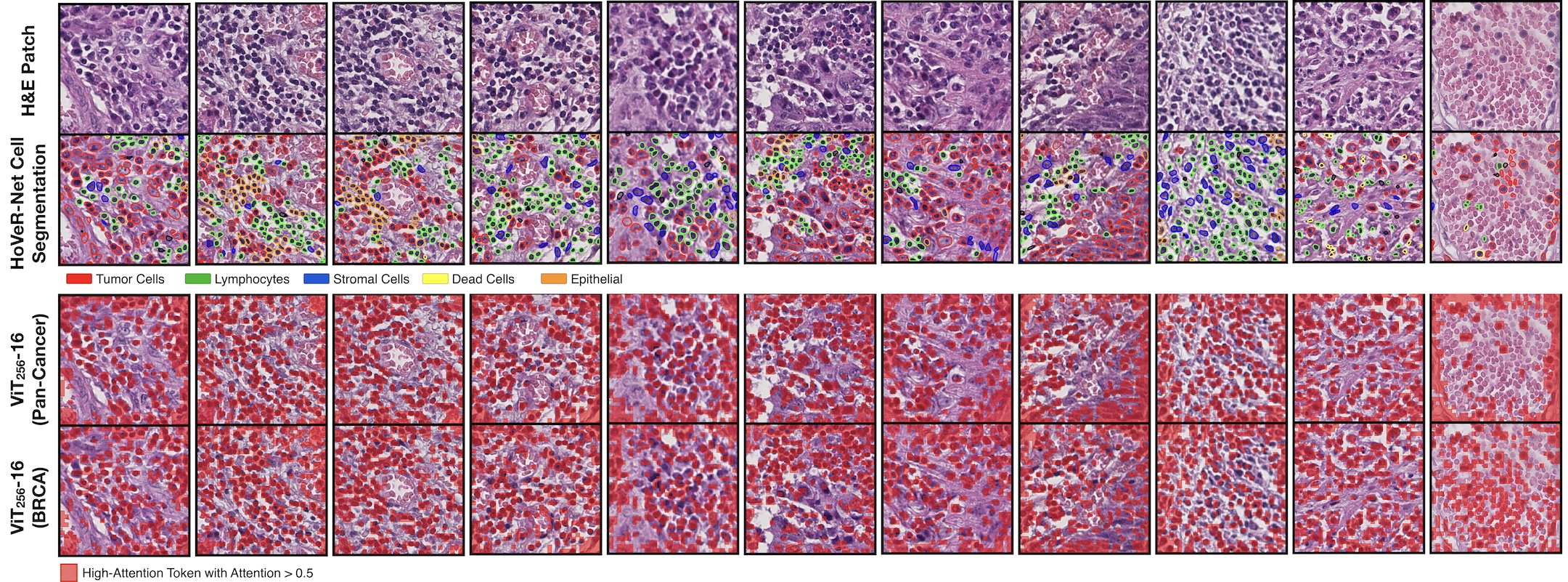
Figure 7: Comparison of Pan-Cancer versus BRCA pretraining in $\operatorname{\mathbf{ViT_{256}\textrm{-}16}}$. For $\operatorname{ViT_{256}\textrm{-}16}_{\text{PF, BRCA, S1}}$ and ViT-16${}_{\text{PF, PANC, S1}}$, we visualize the attention weights for $h=0,3$ respectively which we observe to be good at localizing cells. For both $\operatorname{ViT_{256}\textrm{-}16}$ models, overlayed in ”red” are high-attention visual tokens with attention weights greater than 0.5. In addition, we all show accompanying cell segmentation results from a HoVeR-Net model [31]. Overall, we observe that Pan-Cancer pretraining in $\operatorname{ViT_{256}\textrm{-}16}$ is able to localize tumor and lymphocytes better than BRCA pretraining, with BRCA pretraining attending to blood cells in some instances.

Organ-Specific versus Pan-Cancer Image Pretraining

In comparing $\operatorname{ViT_{256}\textrm{-}16}_{\text{PF, PANC, S1}}$ with $\operatorname{ViT_{256}\textrm{-}16}_{\text{PF, BRCA, S1}}$, briefly, we note that both models have similar performance across most patch-level tasks, with $\operatorname{ViT_{256}\textrm{-}16}_{\text{PF, PANC, S1}}$ performing slightly better on BCSS and BreastPathQ evaluation. In examining global structure of morphological subtypes in CRC-100K, despite not being pretrained on CRC data, $\operatorname{ViT_{256}\textrm{-}16}_{\text{PF, BRCA, S1}}$ is able to preserve global structure better in stroma and mucous subtypes. In Figure 7, we additionally visualize the cell localization results of each ViT model, with $\operatorname{ViT_{256}\textrm{-}16}_{\text{PF, PANC, S1}}$ performing overall better in localizing tumor cells and lymphocytes, with $\operatorname{ViT_{256}\textrm{-}16}_{\text{PF, BRCA, S1}}$ attending more to blood cells.

Feature Concatenation across $\operatorname{\mathbf{ViT_{256}\textrm{-}16}}$ Hidden Layers

Following Caron et al., we also concatenated the $\operatorname{[CLS]}$ tokens from the last four stages of $\operatorname{ViT_{256}\textrm{-}16}$, resulting in a 1536-dim embedding [14]. We observe no improvement in performing feature concatenation.

Concluding Remarks on $\textbf{x}_{256}$ Representations

In addition to having strong representation quality and interpretability mechanisms in finding unique morphological features, a key detail about $\operatorname{ViT_{256}\textrm{-}16}$ is that the embedding dimension is relatively small (with a length of 384), which allows Stage 2 Hierarchical Pretraining and finetuning of $\operatorname{ViT_{4096}\textrm{-}256}$ to be tractable on commercial workstations. Though longer embedding dimensions may lead to better performance on some patch-level tasks, our ultimate goal is in building hierarchical models for slide-level representation learning, which relies on: 1) shorter embedding dimensions, and 2) $[16\times 16]$ cell-level interpretability.

Appendix D Additional Visualizations

Additional visualizations for hierarchical attention maps are shown in Figure 8, 9. Attached in is also a hierarchical attention map for Figure 3 in its native $4096\times 4096$ resolution. Due to space constraints, we created a repository to visualize $\operatorname{ViT_{256}\textrm{-}16}$, $\operatorname{ViT_{4096}\textrm{-}256}$, and hierarchical attention heatmaps at the following link address: https://bit.ly/HIPT-Supplement.

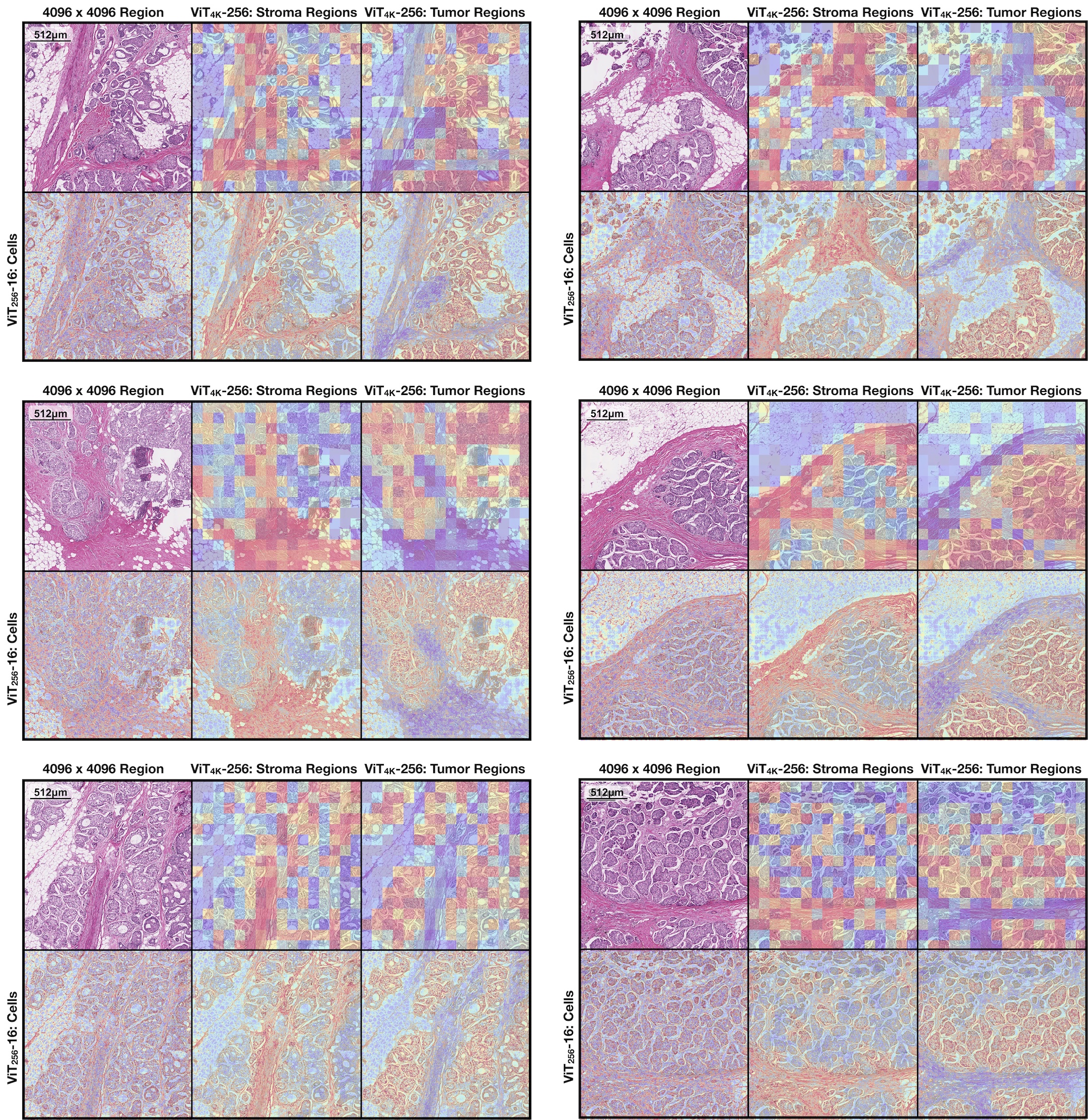
Figure 8: Hierarchical Attention Maps for Invasive Breast Carcinoma (BRCA). Similar to Figure 4, factorized attention distributions of combined $\operatorname{ViT_{256}\textrm{-}16}$ and $\operatorname{ViT_{4096}\textrm{-}256}$ attention distributions are able to localize: 1) invasive tumor cells in demoplastic stroma, 2) tumor cells arranged in larger tumor nest patterns, which is important in distinguishing Invasive Ductal versus Lobular Carcinoma as well as survival outcomes.

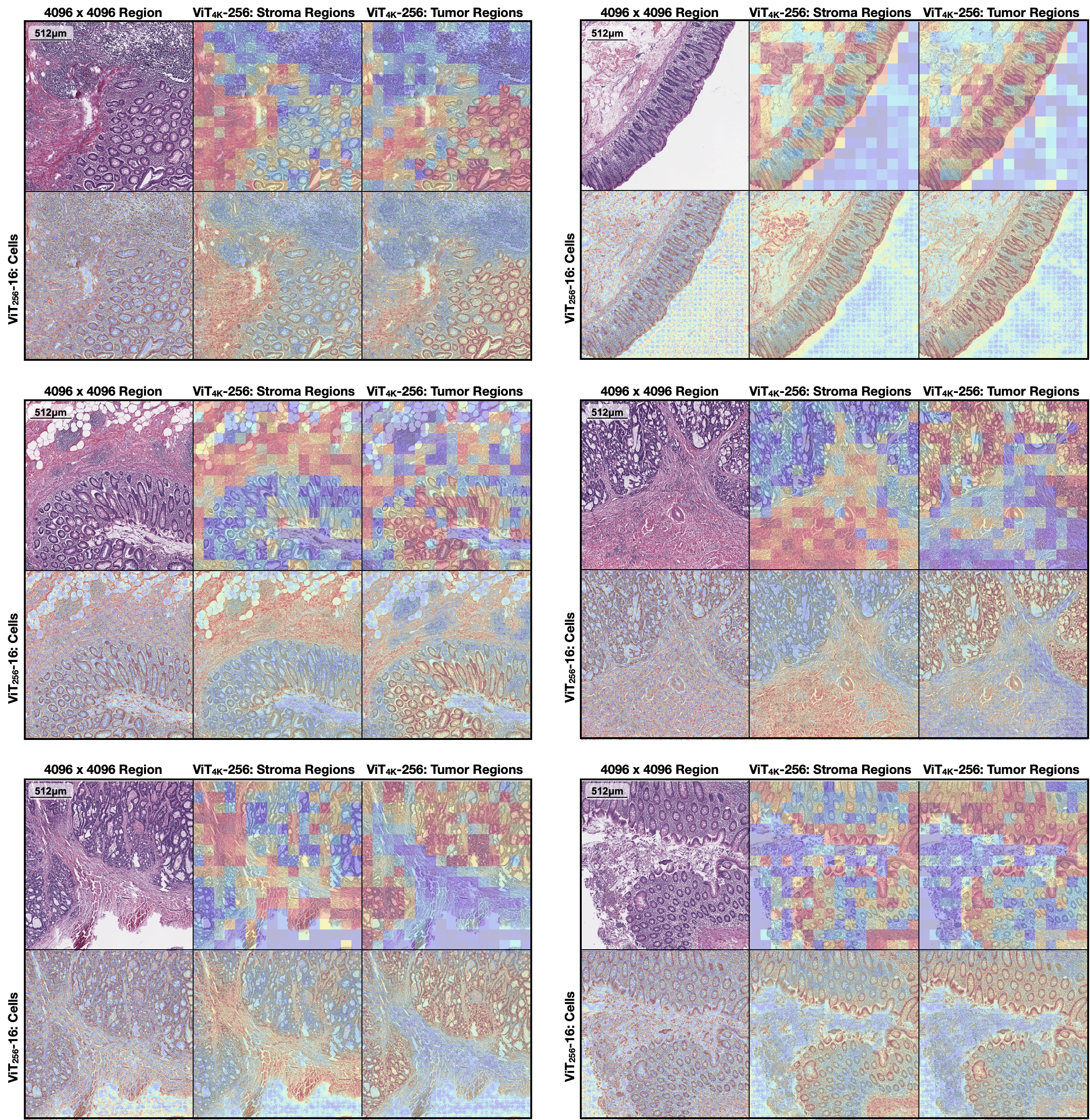
Figure 9: Hierarchical Attention Maps for Colorectal Cancer (CRC). Similar to Figure 4, factorized attention distributions of combined $\operatorname{ViT_{256}\textrm{-}16}$ and $\operatorname{ViT_{4096}\textrm{-}256}$ attention distributions are able to localize: 1) invasive tumor cells in muscle and stromal regions, 2) tumor cells forming poorly-differentiated glands, which are both important prognostic histopathologic biomarkers in determining severity in cancer staging and survival outcomes.

References

- [1] Khalid Abdul Jabbar, Shan E Ahmed Raza, Rachel Rosenthal, Mariam Jamal-Hanjani, Selvaraju Veeriah, Ayse Akarca, Tom Lund, David A Moore, Roberto Salgado, Maise Al Bakir, et al. Geospatial immune variability illuminates differential evolution of lung adenocarcinoma. Nature Medicine, pages 1–9, 2020.
- [2] Shahira Abousamra, David Belinsky, John Van Arnam, Felicia Allard, Eric Yee, Rajarsi Gupta, Tahsin Kurc, Dimitris Samaras, Joel Saltz, and Chao Chen. Multi-class cell detection using spatial context representation. In Proceedings of the IEEE/CVF International Conference on Computer Vision, pages 4005–4014, 2021.
- [3] Mohamed Amgad, Habiba Elfandy, Hagar Hussein, Lamees A Atteya, Mai AT Elsebaie, Lamia S Abo Elnasr, Rokia A Sakr, Hazem SE Salem, Ahmed F Ismail, Anas M Saad, et al. Structured crowdsourcing enables convolutional segmentation of histology images. Bioinformatics, 35(18):3461–3467, 2019.
- [4] Žiga Avsec, Vikram Agarwal, Daniel Visentin, Joseph R Ledsam, Agnieszka Grabska-Barwinska, Kyle R Taylor, Yannis Assael, John Jumper, Pushmeet Kohli, and David R Kelley. Effective gene expression prediction from sequence by integrating long-range interactions. Nature methods, 18(10):1196–1203, 2021.
- [5] Frances R Balkwill, Melania Capasso, and Thorsten Hagemann. The tumor microenvironment at a glance. Journal of cell science, 125(23):5591–5596, 2012.
- [6] Hangbo Bao, Li Dong, Songhao Piao, and Furu Wei. BEit: BERT pre-training of image transformers. In International Conference on Learning Representations, 2022.
- [7] Andrew H Beck, Ankur R Sangoi, Samuel Leung, Robert J Marinelli, Torsten O Nielsen, Marc J Van De Vijver, Robert B West, Matt Van De Rijn, and Daphne Koller. Systematic analysis of breast cancer morphology uncovers stromal features associated with survival. Science Translational Medicine, 3(108):108ra113–108ra113, 2011.
- [8] Babak Ehteshami Bejnordi, Mitko Veta, Paul Johannes Van Diest, Bram Van Ginneken, Nico Karssemeijer, Geert Litjens, Jeroen AWM Van Der Laak, Meyke Hermsen, Quirine F Manson, Maschenka Balkenhol, et al. Diagnostic assessment of deep learning algorithms for detection of lymph node metastases in women with breast cancer. JAMA, 318(22):2199–2210, 2017.
- [9] Joseph Boyd, Mykola Liashuha, Eric Deutsch, Nikos Paragios, Stergios Christodoulidis, and Maria Vakalopoulou. Self-supervised representation learning using visual field expansion on digital pathology. In Proceedings of the IEEE/CVF International Conference on Computer Vision, pages 639–647, 2021.
- [10] Nadia Brancati, Anna Maria Anniciello, Pushpak Pati, Daniel Riccio, Giosuè Scognamiglio, Guillaume Jaume, Giuseppe De Pietro, Maurizio Di Bonito, Antonio Foncubierta, Gerardo Botti, et al. Bracs: A dataset for breast carcinoma subtyping in h&e histology images. arXiv preprint arXiv:2111.04740, 2021.
- [11] Wieland Brendel and Matthias Bethge. Approximating cnns with bag-of-local-features models works surprisingly well on imagenet. In 7th International Conference on Learning Representations, ICLR 2019, New Orleans, LA, USA, May 6-9, 2019. OpenReview.net, 2019.
- [12] Peter J Burt and Edward H Adelson. The laplacian pyramid as a compact image code. In Readings in computer vision, pages 671–679. Elsevier, 1987.
- [13] Gabriele Campanella, Matthew G Hanna, Luke Geneslaw, Allen Miraflor, Vitor Werneck Krauss Silva, Klaus J Busam, Edi Brogi, Victor E Reuter, David S Klimstra, and Thomas J Fuchs. Clinical-grade computational pathology using weakly supervised deep learning on whole slide images. Nature Medicine, 25(8):1301–1309, 2019.
- [14] Mathilde Caron, Hugo Touvron, Ishan Misra, Hervé Jégou, Julien Mairal, Piotr Bojanowski, and Armand Joulin. Emerging properties in self-supervised vision transformers. arXiv preprint arXiv:2104.14294, 2021.
- [15] Joao Carreira, Skanda Koppula, Daniel Zoran, Adria Recasens, Catalin Ionescu, Olivier Henaff, Evan Shelhamer, Relja Arandjelovic, Matt Botvinick, Oriol Vinyals, et al. Hierarchical perceiver. arXiv preprint arXiv:2202.10890, 2022.
- [16] Lyndon Chan, Mahdi S Hosseini, Corwyn Rowsell, Konstantinos N Plataniotis, and Savvas Damaskinos. Histosegnet: Semantic segmentation of histological tissue type in whole slide images. In Proceedings of the IEEE/CVF International Conference on Computer Vision, pages 10662–10671, 2019.
- [17] Richard J Chen and Rahul G Krishnan. Self-supervised vision transformers learn visual concepts in histopathology. Learning Meaningful Representations of Life, NeurIPS 2021, 2022.
- [18] Richard J Chen, Ming Y Lu, Wei-Hung Weng, Tiffany Y Chen, Drew FK Williamson, Trevor Manz, Maha Shady, and Faisal Mahmood. Multimodal co-attention transformer for survival prediction in gigapixel whole slide images. In Proceedings of the IEEE/CVF International Conference on Computer Vision, pages 4015–4025, 2021.
- [19] Ozan Ciga, Tony Xu, and Anne Louise Martel. Self supervised contrastive learning for digital histopathology. Machine Learning with Applications, page 100198, 2021.
- [20] Pierre Courtiol, Charles Maussion, Matahi Moarii, Elodie Pronier, Samuel Pilcer, Meriem Sefta, Pierre Manceron, Sylvain Toldo, Mikhail Zaslavskiy, Nolwenn Le Stang, et al. Deep learning-based classification of mesothelioma improves prediction of patient outcome. Nature Medicine, 25(10):1519–1525, 2019.
- [21] Olivier Dehaene, Axel Camara, Olivier Moindrot, Axel de Lavergne, and Pierre Courtiol. Self-supervision closes the gap between weak and strong supervision in histology. arXiv preprint arXiv:2012.03583, 2020.
- [22] Pinar Demetci, Wei Cheng, Gregory Darnell, Xiang Zhou, Sohini Ramachandran, and Lorin Crawford. Multi-scale inference of genetic trait architecture using biologically annotated neural networks. PLoS genetics, 17(8):e1009754, 2021.
- [23] James A. Diao, Jason K. Wang, Wan Fung Chui, Victoria Mountain, Sai Chowdary Gullapally, Ramprakash Srinivasan, Richard N. Mitchell, Benjamin Glass, Sara Hoffman, Sudha K. Rao, Chirag Maheshwari, Abhik Lahiri, Aaditya Prakash, Ryan McLoughlin, Jennifer K. Kerner, Murray B. Resnick, Michael C. Montalto, Aditya Khosla, Ilan N. Wapinski, Andrew H. Beck, Hunter L. Elliott, and Amaro Taylor-Weiner. Human-interpretable image features derived from densely mapped cancer pathology slides predict diverse molecular phenotypes. Nature Communications, 12(1), Mar. 2021.
- [24] Alexey Dosovitskiy, Lucas Beyer, Alexander Kolesnikov, Dirk Weissenborn, Xiaohua Zhai, Thomas Unterthiner, Mostafa Dehghani, Matthias Minderer, Georg Heigold, Sylvain Gelly, Jakob Uszkoreit, and Neil Houlsby. An image is worth 16x16 words: Transformers for image recognition at scale. In International Conference on Learning Representations, 2021.
- [25] Amelie Echle, Niklas Timon Rindtorff, Titus Josef Brinker, Tom Luedde, Alexander Thomas Pearson, and Jakob Nikolas Kather. Deep learning in cancer pathology: a new generation of clinical biomarkers. British Journal of Cancer, 124(4):686–696, Nov. 2020.
- [26] Harrison Edwards and Amos J. Storkey. Towards a neural statistician. In 5th International Conference on Learning Representations, ICLR 2017, Toulon, France, April 24-26, 2017, Conference Track Proceedings. OpenReview.net, 2017.
- [27] Dumitru Erhan, Aaron Courville, Yoshua Bengio, and Pascal Vincent. Why does unsupervised pre-training help deep learning? In Proceedings of the thirteenth international conference on artificial intelligence and statistics, pages 201–208. JMLR Workshop and Conference Proceedings, 2010.
- [28] Haoqi Fan, Bo Xiong, Karttikeya Mangalam, Yanghao Li, Zhicheng Yan, Jitendra Malik, and Christoph Feichtenhofer. Multiscale vision transformers. In Proceedings of the IEEE/CVF International Conference on Computer Vision, pages 6824–6835, 2021.
- [29] Tianyu Gao, Xingcheng Yao, and Danqi Chen. SimCSE: Simple contrastive learning of sentence embeddings. In Proceedings of the 2021 Conference on Empirical Methods in Natural Language Processing, pages 6894–6910, Online and Punta Cana, Dominican Republic, Nov. 2021. Association for Computational Linguistics.
- [30] Yi Gao, William Liu, Shipra Arjun, Liangjia Zhu, Vadim Ratner, Tahsin Kurc, Joel Saltz, and Allen Tannenbaum. Multi-scale learning based segmentation of glands in digital colonrectal pathology images. In Medical Imaging 2016: Digital Pathology, volume 9791, page 97910M. International Society for Optics and Photonics, 2016.
- [31] Simon Graham, Quoc Dang Vu, Shan E Ahmed Raza, Ayesha Azam, Yee Wah Tsang, Jin Tae Kwak, and Nasir Rajpoot. Hover-net: Simultaneous segmentation and classification of nuclei in multi-tissue histology images. Medical Image Analysis, 58:101563, 2019.
- [32] Kai Han, An Xiao, Enhua Wu, Jianyuan Guo, Chunjing Xu, and Yunhe Wang. Transformer in transformer. Advances in Neural Information Processing Systems, 34, 2021.
- [33] Noriaki Hashimoto, Daisuke Fukushima, Ryoichi Koga, Yusuke Takagi, Kaho Ko, Kei Kohno, Masato Nakaguro, Shigeo Nakamura, Hidekata Hontani, and Ichiro Takeuchi. Multi-scale domain-adversarial multiple-instance cnn for cancer subtype classification with unannotated histopathological images. In Proceedings of the IEEE/CVF conference on computer vision and pattern recognition, pages 3852–3861, 2020.
- [34] Kaiming He, Xinlei Chen, Saining Xie, Yanghao Li, Piotr Dollár, and Ross Girshick. Masked autoencoders are scalable vision learners. arXiv preprint arXiv:2111.06377, 2021.
- [35] Geoffrey Hinton. How to represent part-whole hierarchies in a neural network. arXiv preprint arXiv:2102.12627, 2021.
- [36] Mahdi S Hosseini, Lyndon Chan, Gabriel Tse, Michael Tang, Jun Deng, Sajad Norouzi, Corwyn Rowsell, Konstantinos N Plataniotis, and Savvas Damaskinos. Atlas of digital pathology: A generalized hierarchical histological tissue type-annotated database for deep learning. In Proceedings of the IEEE/CVF Conference on Computer Vision and Pattern Recognition, pages 11747–11756, 2019.
- [37] Le Hou, Vu Nguyen, Ariel B Kanevsky, Dimitris Samaras, Tahsin M Kurc, Tianhao Zhao, Rajarsi R Gupta, Yi Gao, Wenjin Chen, David Foran, et al. Sparse autoencoder for unsupervised nucleus detection and representation in histopathology images. Pattern Recognition, 86:188–200, 2019.
- [38] Le Hou, Dimitris Samaras, Tahsin M Kurc, Yi Gao, James E Davis, and Joel H Saltz. Patch-based convolutional neural network for whole slide tissue image classification. In Proceedings of the IEEE/CVF Conference on Computer Vision and Pattern Recognition, pages 2424–2433, 2016.
- [39] Maximilian Ilse, Jakub Tomczak, and Max Welling. Attention-based deep multiple instance learning. In Proceedings of the 35th International Conference on Machine Learning, pages 2132–2141, 2018.
- [40] Sajid Javed, Arif Mahmood, Muhammad Moazam Fraz, Navid Alemi Koohbanani, Ksenija Benes, Yee-Wah Tsang, Katherine Hewitt, David Epstein, David Snead, and Nasir Rajpoot. Cellular community detection for tissue phenotyping in colorectal cancer histology images. Medical image analysis, 63:101696, 2020.
- [41] John Jumper, Richard Evans, Alexander Pritzel, Tim Green, Michael Figurnov, Olaf Ronneberger, Kathryn Tunyasuvunakool, Russ Bates, Augustin Žídek, Anna Potapenko, et al. Highly accurate protein structure prediction with alphafold. Nature, 596(7873):583–589, 2021.
- [42] Jakob Nikolas Kather, Cleo-Aron Weis, Francesco Bianconi, Susanne M Melchers, Lothar R Schad, Timo Gaiser, Alexander Marx, and Frank Gerrit Zöllner. Multi-class texture analysis in colorectal cancer histology. Scientific reports, 6(1):1–11, 2016.
- [43] Jan J Koenderink. The structure of images. Biological cybernetics, 50(5):363–370, 1984.
- [44] Navid Alemi Koohbanani, Balagopal Unnikrishnan, Syed Ali Khurram, Pavitra Krishnaswamy, and Nasir Rajpoot. Self-path: Self-supervision for classification of pathology images with limited annotations. IEEE Transactions on Medical Imaging, 2021.
- [45] Han Le, Rajarsi Gupta, Le Hou, Shahira Abousamra, Danielle Fassler, Luke Torre-Healy, Richard A Moffitt, Tahsin Kurc, Dimitris Samaras, Rebecca Batiste, et al. Utilizing automated breast cancer detection to identify spatial distributions of tumor-infiltrating lymphocytes in invasive breast cancer. The American journal of pathology, 190(7):1491–1504, 2020.
- [46] Bin Li, Yin Li, and Kevin W Eliceiri. Dual-stream multiple instance learning network for whole slide image classification with self-supervised contrastive learning. In Proceedings of the IEEE/CVF Conference on Computer Vision and Pattern Recognition, pages 14318–14328, 2021.
- [47] Chunyuan Li, Jianwei Yang, Pengchuan Zhang, Mei Gao, Bin Xiao, Xiyang Dai, Lu Yuan, and Jianfeng Gao. Efficient self-supervised vision transformers for representation learning. In International Conference on Learning Representations, 2022.
- [48] Guohao Li, Matthias Muller, Ali Thabet, and Bernard Ghanem. Deepgcns: Can gcns go as deep as cnns? In Proceedings of the IEEE/CVF International Conference on Computer Vision, pages 9267–9276, 2019.
- [49] Michelle M Li, Kexin Huang, and Marinka Zitnik. Representation learning for networks in biology and medicine: advancements, challenges, and opportunities. arXiv preprint arXiv:2104.04883, 2021.
- [50] Ruoyu Li, Jiawen Yao, Xinliang Zhu, Yeqing Li, and Junzhou Huang. Graph cnn for survival analysis on whole slide pathological images. In International Conference on Medical Image Computing and Computer-Assisted Intervention, pages 174–182. Springer, 2018.
- [51] Jianfang Liu, Tara Lichtenberg, Katherine A Hoadley, Laila M Poisson, Alexander J Lazar, Andrew D Cherniack, Albert J Kovatich, Christopher C Benz, Douglas A Levine, Adrian V Lee, et al. An integrated tcga pan-cancer clinical data resource to drive high-quality survival outcome analytics. Cell, 173(2):400–416, 2018.
- [52] Ze Liu, Yutong Lin, Yue Cao, Han Hu, Yixuan Wei, Zheng Zhang, Stephen Lin, and Baining Guo. Swin transformer: Hierarchical vision transformer using shifted windows. In Proceedings of the IEEE/CVF International Conference on Computer Vision, pages 10012–10022, 2021.
- [53] Ming Y Lu, Tiffany Y Chen, Drew FK Williamson, Melissa Zhao, Maha Shady, Jana Lipkova, and Faisal Mahmood. Ai-based pathology predicts origins for cancers of unknown primary. Nature, 594(7861):106–110, 2021.
- [54] Ming Y Lu, Drew FK Williamson, Tiffany Y Chen, Richard J Chen, Matteo Barbieri, and Faisal Mahmood. Data efficient and weakly supervised computational pathology on whole slide images. Nature Biomedical Engineering, 2020.
- [55] Joseph A Ludwig and John N Weinstein. Biomarkers in cancer staging, prognosis and treatment selection. Nature Reviews Cancer, 5(11):845–856, 2005.
- [56] Jianzhu Ma, Michael Ku Yu, Samson Fong, Keiichiro Ono, Eric Sage, Barry Demchak, Roded Sharan, and Trey Ideker. Using deep learning to model the hierarchical structure and function of a cell. Nature methods, 15(4):290–298, 2018.
- [57] Niccolò Marini, Sebastian Otálora, Francesco Ciompi, Gianmaria Silvello, Stefano Marchesin, Simona Vatrano, Genziana Buttafuoco, Manfredo Atzori, and Henning Müller. Multi-scale task multiple instance learning for the classification of digital pathology images with global annotations. In MICCAI Workshop on Computational Pathology, pages 170–181. PMLR, 2021.
- [58] Andriy Marusyk, Vanessa Almendro, and Kornelia Polyak. Intra-tumour heterogeneity: a looking glass for cancer? Nature Reviews Cancer, 12(5):323–334, 2012.
- [59] Zhu Meng, Zhicheng Zhao, Fei Su, and Limei Guo. Hierarchical spatial pyramid network for cervical precancerous segmentation by reconstructing deep segmentation networks. In Proceedings of the IEEE/CVF Conference on Computer Vision and Pattern Recognition, pages 3738–3745, 2021.
- [60] Pushpak Pati, Guillaume Jaume, Lauren Alisha Fernandes, Antonio Foncubierta-Rodríguez, Florinda Feroce, Anna Maria Anniciello, Giosue Scognamiglio, Nadia Brancati, Daniel Riccio, Maurizio Di Bonito, et al. Hact-net: A hierarchical cell-to-tissue graph neural network for histopathological image classification. In Uncertainty for Safe Utilization of Machine Learning in Medical Imaging, and Graphs in Biomedical Image Analysis, pages 208–219. Springer, 2020.
- [61] Pushpak Pati, Guillaume Jaume, Antonio Foncubierta-Rodríguez, Florinda Feroce, Anna Maria Anniciello, Giosue Scognamiglio, Nadia Brancati, Maryse Fiche, Estelle Dubruc, Daniel Riccio, et al. Hierarchical graph representations in digital pathology. Medical image analysis, 75:102264, 2022.
- [62] Nicholas Petrick, Shazia Akbar, Kenny H Cha, Sharon Nofech-Mozes, Berkman Sahiner, Marios A Gavrielides, Jayashree Kalpathy-Cramer, Karen Drukker, Anne L Martel, et al. Spie-aapm-nci breastpathq challenge: an image analysis challenge for quantitative tumor cellularity assessment in breast cancer histology images following neoadjuvant treatment. Journal of Medical Imaging, 8(3):034501, 2021.
- [63] Azriel Rosenfeld and Mark Thurston. Edge and curve detection for visual scene analysis. IEEE Transactions on computers, 100(5):562–569, 1971.
- [64] Charlie Saillard, Olivier Dehaene, Tanguy Marchand, Olivier Moindrot, Aurélie Kamoun, Benoit Schmauch, and Simon Jegou. Self supervised learning improves dMMR/MSI detection from histology slides across multiple cancers. In COMPAY 2021: The third MICCAI workshop on Computational Pathology, 2021.
- [65] Joel Saltz, Rajarsi Gupta, Le Hou, Tahsin Kurc, Pankaj Singh, Vu Nguyen, Dimitris Samaras, Kenneth R Shroyer, Tianhao Zhao, Rebecca Batiste, et al. Spatial organization and molecular correlation of tumor-infiltrating lymphocytes using deep learning on pathology images. Cell reports, 23(1):181–193, 2018.
- [66] Zhuchen Shao, Hao Bian, Yang Chen, Yifeng Wang, Jian Zhang, Xiangyang Ji, et al. Transmil: Transformer based correlated multiple instance learning for whole slide image classification. Advances in Neural Information Processing Systems, 34, 2021.
- [67] Oriane Siméoni, Gilles Puy, Huy V. Vo, Simon Roburin, Spyros Gidaris, Andrei Bursuc, Patrick Pérez, Renaud Marlet, and Jean Ponce. Localizing objects with self-supervised transformers and no labels. In Proceedings of the British Machine Vision Conference (BMVC), November 2021.
- [68] Ole-Johan Skrede, Sepp De Raedt, Andreas Kleppe, Tarjei S Hveem, Knut Liestøl, John Maddison, Hanne A Askautrud, Manohar Pradhan, John Arne Nesheim, Fritz Albregtsen, et al. Deep learning for prediction of colorectal cancer outcome: a discovery and validation study. The Lancet, 395(10221):350–360, 2020.
- [69] Daniel E Spratt, Tiffany Chan, Levi Waldron, Corey Speers, Felix Y Feng, Olorunseun O Ogunwobi, and Joseph R Osborne. Racial/ethnic disparities in genomic sequencing. JAMA oncology, 2(8):1070–1074, 2016.
- [70] David Tellez, Geert Litjens, Jeroen van der Laak, and Francesco Ciompi. Neural image compression for gigapixel histopathology image analysis. IEEE Transactions on Pattern Analysis and Machine Intelligence, 2019.
- [71] Hugo Touvron, Matthieu Cord, Matthijs Douze, Francisco Massa, Alexandre Sablayrolles, and Hervé Jégou. Training data-efficient image transformers & distillation through attention. In International Conference on Machine Learning, pages 10347–10357. PMLR, 2021.
- [72] Jeroen van der Laak, Francesco Ciompi, and Geert Litjens. No pixel-level annotations needed. Nature biomedical engineering, 3(11):855–856, 2019.
- [73] Ashish Vaswani, Noam Shazeer, Niki Parmar, Jakob Uszkoreit, Llion Jones, Aidan N Gomez, Łukasz Kaiser, and Illia Polosukhin. Attention is all you need. Advances in neural information processing systems, 30, 2017.
- [74] Wenhai Wang, Enze Xie, Xiang Li, Deng-Ping Fan, Kaitao Song, Ding Liang, Tong Lu, Ping Luo, and Ling Shao. Pyramid vision transformer: A versatile backbone for dense prediction without convolutions. In Proceedings of the IEEE/CVF International Conference on Computer Vision, pages 568–578, 2021.
- [75] Ellery Wulczyn, David F. Steiner, Melissa Moran, Markus Plass, Robert Reihs, Fraser Tan, Isabelle Flament-Auvigne, Trissia Brown, Peter Regitnig, Po-Hsuan Cameron Chen, Narayan Hegde, Apaar Sadhwani, Robert MacDonald, Benny Ayalew, Greg S. Corrado, Lily H. Peng, Daniel Tse, Heimo Müller, Zhaoyang Xu, Yun Liu, Martin C. Stumpe, Kurt Zatloukal, and Craig H. Mermel. Interpretable survival prediction for colorectal cancer using deep learning. npj Digital Medicine, 4(1), Apr. 2021.
- [76] Ellery Wulczyn, David F Steiner, Zhaoyang Xu, Apaar Sadhwani, Hongwu Wang, Isabelle Flament-Auvigne, Craig H Mermel, Po-Hsuan Cameron Chen, Yun Liu, and Martin C Stumpe. Deep learning-based survival prediction for multiple cancer types using histopathology images. PLoS One, 15(6):e0233678, 2020.
- [77] Gang Xu, Zhigang Song, Zhuo Sun, Calvin Ku, Zhe Yang, Cancheng Liu, Shuhao Wang, Jianpeng Ma, and Wei Xu. Camel: A weakly supervised learning framework for histopathology image segmentation. In Proceedings of the IEEE/CVF International Conference on Computer Vision, pages 10682–10691, 2019.
- [78] Zichao Yang, Diyi Yang, Chris Dyer, Xiaodong He, Alex Smola, and Eduard Hovy. Hierarchical attention networks for document classification. In Proceedings of the 2016 conference of the North American chapter of the association for computational linguistics: human language technologies, pages 1480–1489, 2016.
- [79] Jiawen Yao, Xinliang Zhu, and Junzhou Huang. Deep multi-instance learning for survival prediction from whole slide images. In International Conference on Medical Image Computing and Computer-Assisted Intervention, pages 496–504. Springer, 2019.
- [80] Jiawen Yao, Xinliang Zhu, Jitendra Jonnagaddala, Nicholas Hawkins, and Junzhou Huang. Whole slide images based cancer survival prediction using attention guided deep multiple instance learning networks. Medical Image Analysis, 65:101789, 2020.
- [81] Shekoufeh Gorgi Zadeh and Matthias Schmid. Bias in cross-entropy-based training of deep survival networks. IEEE Transactions on Pattern Analysis and Machine Intelligence, 2020.
- [82] Manzil Zaheer, Satwik Kottur, Siamak Ravanbakhsh, Barnabas Poczos, Ruslan Salakhutdinov, and Alexander Smola. Deep sets. Advances in Neural Information Processing Systems, 2017.
- [83] Pengchuan Zhang, Xiyang Dai, Jianwei Yang, Bin Xiao, Lu Yuan, Lei Zhang, and Jianfeng Gao. Multi-scale vision longformer: A new vision transformer for high-resolution image encoding. In Proceedings of the IEEE/CVF International Conference on Computer Vision, pages 2998–3008, 2021.
- [84] Xingxing Zhang, Furu Wei, and Ming Zhou. HIBERT: Document level pre-training of hierarchical bidirectional transformers for document summarization. In Proceedings of the 57th Annual Meeting of the Association for Computational Linguistics, pages 5059–5069, Florence, Italy, July 2019. Association for Computational Linguistics.
- [85] Zizhao Zhang, Han Zhang, Long Zhao, Ting Chen, Sercan Arik, and Tomas Pfister. Nested hierarchical transformer: Towards accurate, data-efficient and interpretable visual understanding. In AAAI Conference on Artificial Intelligence (AAAI), 2022, 2022.
- [86] Yu Zhao, Fan Yang, Yuqi Fang, Hailing Liu, Niyun Zhou, Jun Zhang, Jiarui Sun, Sen Yang, Bjoern Menze, Xinjuan Fan, et al. Predicting lymph node metastasis using histopathological images based on multiple instance learning with deep graph convolution. In Proceedings of the IEEE/CVF Conference on Computer Vision and Pattern Recognition, pages 4837–4846, 2020.
- [87] Xinliang Zhu, Jiawen Yao, Feiyun Zhu, and Junzhou Huang. Wsisa: Making survival prediction from whole slide histopathological images. In Proceedings of the IEEE/CVF Conference on Computer Vision and Pattern Recognition, pages 7234–7242, 2017.