Virtual Homogeneity Learning: Defending against Data Heterogeneity in Federated Learning

Abstract

In federated learning (FL), model performance typically suffers from client drift induced by data heterogeneity, and mainstream works focus on correcting client drift. We propose a different approach named virtual homogeneity learning (VHL) to directly “rectify” the data heterogeneity. In particular, VHL conducts FL with a virtual homogeneous dataset crafted to satisfy two conditions: containing no private information and being separable. The virtual dataset can be generated from pure noise shared across clients, aiming to calibrate the features from the heterogeneous clients. Theoretically, we prove that VHL can achieve provable generalization performance on the natural distribution. Empirically, we demonstrate that VHL endows FL with drastically improved convergence speed and generalization performance. VHL is the first attempt towards using a virtual dataset to address data heterogeneity, offering new and effective means to FL.

1 Introduction

Federated learning (FL) (McMahan et al., 2017) has emerged as an important paradigm that enables decentralized data collection and model training. In the FL scenario, a large number of clients collaboratively train a shared model without sharing their natural (or private) data (Kairouz et al., 2021), enabling various real-world applications (Yang et al., 2018; Hsu et al., 2020; Luo et al., 2019). However, FL faces heterogeneity challenges caused by Non-IID data distributions from different clients as well as their diversity of computing and communication capabilities (Li et al., 2020a; Zhao et al., 2018; Hsu et al., 2020). Severe heterogeneity can easily cause client drift (Karimireddy et al., 2020), leading to unstable convergence (Li et al., 2020b) and poor model performance (Wang et al., 2020; Zhao et al., 2018).

To tackle federated heterogeneity, the first FL algorithm, FedAvg (McMahan et al., 2017), proposes to conduct more local computations and fewer communications during training. Though FedAvg addresses the diversity of computing and communication, the client drift induced by the Non-IID data distribution (data heterogeneity) has significant negative impact on FedAvg (Li et al., 2020a; Karimireddy et al., 2020; Li et al., 2020b; Wang et al., 2020; Luo et al., 2021). To address client drift, many efforts have been devoted to designing new learning paradigms, either on the client side, e.g., local training strategy (Li et al., 2020a; Karimireddy et al., 2020), or on the server side, e.g., model aggregation strategy (Yurochkin et al., 2019; Chen & Chao, 2020). However, a recent benchmark work (Li et al., 2021a) shows that FedAvg can outperform its variants in many experimental settings. This reveals that it is challenging for a single method to address the client drift problem in multiple scenarios, reflecting the notoriety and subtlety of client drift. Therefore, addressing client drift remains a fundamental challenge of FL (Kairouz et al., 2021).

Another exciting direction is to directly “rectify” the cause of client drift, i.e., data heterogeneity. Specifically, sharing a small portion of private data (Zhao et al., 2018) or the private statistical information (Shin et al., 2020; Yoon et al., 2021) can make data located in different clients more homogeneous. Nonetheless, the data sharing approach exposes FL to the danger of privacy leakage. Although differential privacy is a competitive candidate for avoiding privacy leakage, employing differential privacy can cause performance degradation (Tramer & Boneh, 2021). All these challenges motivate the following fundamental question:

Is it possible to defend against data heterogeneity in FL systems by sharing data containing no private information?

In this work, we provide an affirmative answer to the question by proposing a novel approach, called virtual homogeneity learning (VHL). The key insight of VHL is that introducing more homogeneous data shared across clients can reduce the data heterogeneity (Jeong et al., 2018). Specifically, VHL constructs a new rectified dataset for each client by sharing a virtual homogeneous dataset among all clients, which is independent of the natural datasets.

The key challenge of VHL is how to generate the virtual dataset to benefit model performance. Intuitively, combining an out-of-distribution dataset with the original data may sacrifice the generalization performance in different aspects such as distribution shift (Pan & Yang, 2009; Ben-David et al., 2010), noisy labels (Frénay & Verleysen, 2013), and garbage data (Polyzotis et al., 2017). In practice, it is challenging to sample data from the natural distribution for constructing a virtual dataset. Hence, introducing much virtual data drawn from a different distribution will cause the training distribution different from the test distribution, i.e., distribution shift, leading to poor generalization performance on the test set (Pan & Yang, 2009; Ben-David et al., 2010). Thus, the distribution shift is one crucial detrimental impact of introducing virtual datasets.

Fortunately, we can access both the labeled virtual dataset, i.e., source domain, and the labeled natural dataset, i.e., target domain, so that we can mitigate the distribution shift through the lens of domain adaptation (DA) (Pan & Yang, 2009; Ben-David et al., 2007; Ganin et al., 2016). In particular, we propose matching the conditional distribution of the source and target domains. Our theoretical analysis shows that matching the virtual and natural distributions conditioned on label information can achieve provable generalization performance. Moreover, this can be instantiated by pulling natural and virtual data features from the same class together, as depicted in Figure 1. To show the efficacy of VHL, we apply VHL in several popular FL algorithms including FedAvg, FedProx, SCAFFOLD, and FedNova on four datasets. Our experimental results show that VHL can boost the generalization ability and the convergence speed.

Our main contributions include:

1. We raise a fundamental question to explore how to reduce data heterogeneity in FL by sharing data that contains no private information.

2. To answer the question, we propose virtual homogeneity learning (VHL), making the first attempt to use virtual datasets to defend against data heterogeneity. To avoid the distribution shift induced by virtual datasets, VHL calibrates natural data features with that of virtual data, inspired by the rationale of domain adaptation.

3. Through comprehensive experiments, we demonstrate that VHL can drastically benefit the convergence speed and the generalization performance of FL models.

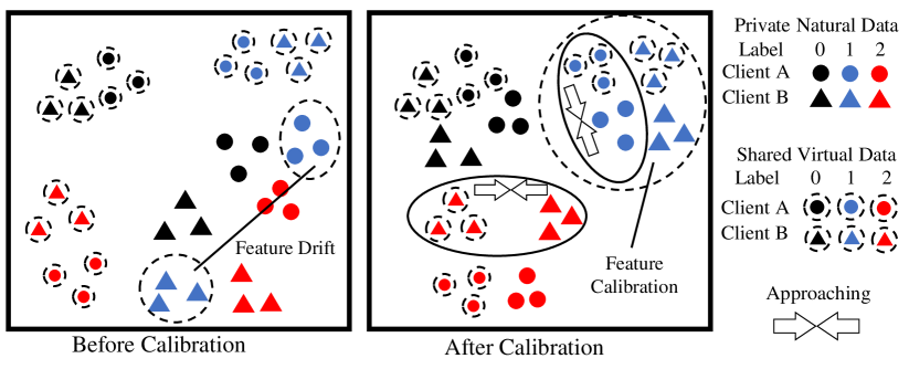
Figure 1: Feature distribution of different clients. Circle and triangle points represent data on client A and B, respectively. Points surrounded by a dotted circle represent the virtual data. Different colors represent data of different labels. After local training (left), the features of private natural data of the same label on different clients are far away from others, but features of shared virtual data of the same label are close to others. Figure 2 in section 5 shows the experimental observation of this Figure.

2 Preliminaries

2.1 Federated Learning

Federated learning aims to collaboratively train a global model parameterized by $w$ while omitting the need to access private data distributed over many clients (McMahan et al., 2017; Kairouz et al., 2021). Formally, FL aims to minimize a global objective function $J(w)$:

$$\min_{w}J(w)\triangleq\sum_{k=1}^{K}p_{k}J_{k}(w),$$ (1)

where $K$ stands for the total number of clients, $p_{k}\geq 0$ is the weight of the $k$-th client such that $\sum_{k=1}^{K}p_{k}=1$, and $J_{k}(w)$ is the local objective defined as:

$$J_{k}(w)\triangleq\mathbb{E}_{(x,y)\sim\mathcal{P}_{k}(x,y)}\ell(f(x;w),y).$$ (2)

Here, we denote $\mathcal{P}_{k}(x,y)$ as the joint distribution of data in client $k$, $\ell(\cdot,\cdot)$ as the loss function, e.g., cross-entropy loss, and $f=\phi\circ\rho$ as the prediction with $\phi$ being the feature extractor as well as $\rho$ the predictor, e.g., classifier for classification tasks.

A common optimization strategy proceeds through the communication between clients and the server round-by-round. In particular, the central server broadcasts the model $w^{r}$ to all selected clients $\mathcal{S}^{r}$ at round $r$ and then each client performs $E$ ($E\geq 1$) local updates, e.g., for the $k$-th client:

$$w_{k,j+1}^{r}\leftarrow w_{k,j}^{r}-\eta_{k,j}\nabla J_{k}(w_{k,j}^{r}),j=0,1,\cdots,E-1,$$

where $w_{k,j}^{r}$ represents the $j$-th updates, i.e., $w_{k,0}^{r}=w^{r}$, and $\eta_{k,j}$ is the learning rate. In the end of round $r$, all selected clients send the optimized parameter back to the server, and the central server performs a certain aggregation operation:

$$w^{r+1}\leftarrow\text{AGGREGATE}(\cup_{k\in\mathcal{S}^{r}}w_{k,E-1}^{r}),$$ (3)

where the AGGREGATE operation is typically instantiated in a simple yet effective averaging manner (McMahan et al., 2017):

$$w^{r+1}\leftarrow\sum_{k\in\mathcal{S}^{r}}p_{k}w_{k,E-1}^{r},\ p_{k}=\frac{n_{k}}{\sum_{i\in\mathcal{S}^{r}}n_{i}},$$

with $n_{k}$ being the number of samples on the $k$-th client.

2.2 Domain Adaptation

Domain adaptation approaches aim to solve the problem where the training and test data are drawn from different distributions (Pan & Yang, 2009). To perform domain adaptation, three assumptions are imposed on how distributions change across domains, i.e.., distribution shifts stem from: $\mathcal{P}(x)$, i.e., covariate shift (Ben-David et al., 2010; Pan et al., 2010), $\mathcal{P}(y|x)$, i.e., conditional shift (Zhang et al., 2013; Gong et al., 2016), or both, i.e., dataset shift (Quiñonero-Candela et al., 2008; Long et al., 2013).

One widely adopted strategy is to minimize the distribution discrepancy between the source distribution $\mathcal{P}_{S}$ and the target distribution $\mathcal{P}_{T}$ by finding a feature extractor $\phi$, such that the source and target domains have similar distributions in the learned feature space (Ganin et al., 2016; Zhao et al., 2019; Long et al., 2017). For the covariate shift assumption, the marginal distribution discrepancy is minimized for reducing generalization risk on the target domain (Ganin et al., 2016):

$$d\left(\mathcal{P}_{S}\left(\phi\left(x\right)\right),\mathcal{P}_{T}\left(\phi\left(x\right)\right)\right),$$

where $d$ is a measure of distribution discrepancy. For the conditional shift assumption, the distribution discrepancy is usually conditioned on the label (Gong et al., 2016):

$$d\left(\mathcal{P}_{S}\left(\phi\left(x\right)|y\right),\mathcal{P}_{T}\left(\phi\left(x\right)|y\right)\right),$$

where $y$ denotes the label. For the most challenging dataset shift, the joint distribution discrepancy is usually employed:

$$d\left(\mathcal{P}_{S}\left(\phi\left(x\right),y\right),\mathcal{P}_{T}\left(\phi\left(x\right),y\right)\right).$$

In this paper, we regard the virtual distribution as the source domain and the natural distribution as the target domain.

3 Virtual Homogeneity Learning

This section gives a detailed description of how virtual heterogeneity learning (VHL) promotes federated learning (FL) by mitigating data heterogeneity with a virtual dataset.

3.1 Heterogeneity Mitigation

Clients in FL systems usually collect data independently, where the data distribution can vary with clients (Kairouz et al., 2021). Hence, data heterogeneity stems from the discrepancy in the data held by the clients. A straightforward solution to mitigate data heterogeneity is to send an extra common dataset to each client and minimize the local objective with both the local data and the shared data.

Unfortunately, the underlying assumption of data sharing is that these extra data are drwan from the natural distribution, because using arbitrary noisy or garbage data to train models produces poor generalization performance (Frénay & Verleysen, 2013; Polyzotis et al., 2017). However, it is not realistic due to the privacy concern. That is, collecting and sharing data from the natural distribution are challenging and will expose FL to the danger of privacy leakage.

To address the challenge, we propose introducing a virtual dataset to reduce data heterogeneity such that the shared virtual data contains no private information and avoids the performance degradation of FL models on the natural dataset. Specifically, we first introduce a dataset collected independently of the natural data to bypass the private information concerns. Then, we expect that models learned from the virtual dataset can perform well on the natural distribution.

3.2 Feature Calibration

The key to promoting FL with a virtual dataset is calibrating the natural feature distribution and the virtual feature distribution. It is effortless to collect data independent of the natural data. For example, the virtual dataset can be generated from pure noise, e.g., Gaussian noise and structural noise drawn from untrained style-GAN (Karras et al., 2019). Thus, the critical challenge is how to ensure that the knowledge learned from the virtual dataset can be transferred to the natural dataset. Drawing inspiration from domain adaptation, we consider the virtual dataset as the source domain and the natural dataset as the target domain and perform domain adaptation to reduce the generalization risk of natural distribution. Built upon the rationale of domain adaptation, we thus propose calibrating these two distributions in the feature space.

The virtual data are crafted independent of the natural data, leading to dataset shift (Quiñonero-Candela et al., 2008; Long et al., 2013) rather than covariate shift (Ben-David et al., 2010) or conditional shift (Zhang et al., 2013). Note that, the virtual data (domain) is different from the heterogeneous domain studied in (Liu et al., 2020), because the virtual dataset is arbitrarily constructed, e.g., pure noise. To tackle the challenging dataset shift, advanced methods (Long et al., 2013, 2017; Lei et al., 2021) follow the rational of domain adaptation to match the joint distribution. Inspired by these approaches, we propose matching the virtual and natural distributions conditioned on the label information to mitigate the adverse impact induced by distribution shift. Thanks to the flexibility of constructing virtual dataset, we can collect virtual data such that the virtual and natural distribution have the same label distributions. Consequently, the joint distribution discrepancy minimization is reduced to the problem of conditional distribution minimization. Specifically, we introduce a conditional distribution mismatch penalty to alleviating the dataset shift:

$$\begin{split}\mathbb{E}_{(x,y)\sim\mathcal{P}_{k}}\ell&\left(\rho\circ\phi\left(x\right),y\right)+\mathbb{E}_{(x,y)\sim\mathcal{P}_{v}}\ell\left(\rho\circ\phi\left(x\right),y\right)\\ +\ &\lambda\mathbb{E}_{y}d\left(\mathcal{P}_{k}\left(\phi\left(x\right)|y\right),\mathcal{P}_{v}\left(\phi\left(x\right)|y\right)\right),\end{split}$$ (4)

where $\mathcal{P}_{v}$ denotes the virtual distribution, e.g., a Gaussian distribution, $\rho\circ\phi=f$ stands for the local model, $\mathcal{P}_{k}\left(\phi\left(x\right)|y\right)$ is the feature distribution obtained by applying the feature extractor $\phi$ to a random variable $x\sim\mathcal{P}_{k}(x|y)$ given label $y$, and $\lambda$ is a hyperparameter. Similarly, $\mathcal{P}_{v}\left(\phi\left(x\right)|y\right)$ is the feature distribution obtained on $x\sim\mathcal{P}_{v}(x|y)$. The penalty $d\left(\mathcal{P}_{k}\left(\phi\left(x\right)|y\right),\mathcal{P}_{v}\left(\phi\left(x\right)|y\right)\right)$ encourages the feature extractor to make the data sampled from different distributions, i.e., $\mathcal{P}_{k}$ and $\mathcal{P}_{v}$, having the same conditional feature distribution.

3.3 Analysis

The insight of VHL is depicted in Figure 1. After local training of each round, the features of natural data in each category on different clients are far away from others, but the features of virtual data in each category are relatively close to others. Thus, pulling the natural feature towards the virtual feature with the same label can contribute to local models having similar features for each category, which is consistent with our empirical observation shown in Figure 2.

To provide a theoretical justification on the effectiveness of the proposed local objective function with distribution mismatch penalty, we analyze the relationship between the generalization performance and the misalignment between domains theoretically for classification tasks. To the best of our knowledge, we are the first to study the relationship for classification tasks. For example, the theoretical conclusions derived in (Lei et al., 2021) are mainly focused on regression problems and only empirical supports are given in (Long et al., 2013, 2017).

In light of the margin theory (Koltchinskii & Panchenko, 2002) that maximizing the margin between data points and the decision boundary achieves strong generalization performance, we first introduce the definition of statistical margin to measure the generalization performance before stating the main theorem.

Definition 3.1.

(Statistical margin.) We define statistical margin for a classifier $f$ on a distribution $\mathcal{P}$ with a distance metric $m$: $\textit{SM}_{m}(f,\mathcal{P})=\mathbb{E}_{(x,y)\sim\mathcal{P}}\inf_{f(x^{\prime})\neq y}m(x^{\prime},x)$.

The defined statistical margin quantifies the degree of generalization performance. Hence, we can use it to quantify models’ generalization performance on the target distribution, where the models are learned from the virtual dataset. In particular, the problem of achieving strong generalization performance is rephrased to maximizing the statistical margin:

$$\mathbb{E}_{f:=\textit{VHL}(\mathcal{P}_{v}(x,y))}\textit{SM}_{m}(f,\mathcal{P}(x,y)),$$ (5)

where $f:=\textit{VHL}(\mathcal{P}_{v}(x,y))$ means that the model $f$ is learned on the distribution $\mathcal{P}_{v}(x,y)$ using Eq. 4, $\textit{SM}_{m}(f,\mathcal{P}(x,y))$ represents that the generalization performance of $f$ is evaluated on the distribution $\mathcal{P}(x,y)$.

Built upon Definition 3.1 and Eq. 5, we are ready to state the following theorem (proof can be found in Appendix A).

Theorem 3.2.

Let $f=\phi\circ\rho$ be a neural network decompose of a feature extractor $\phi$ and a classifier $\rho$, $\mathcal{P}(x,y)$ and $\mathcal{P}_{v}(x,y)$ are two separable distributions with identical label distributions. Then, learning $f$ with the proposed distribution mismatch penalty, i.e., Eq. 4 elicits an model with bounded statistical margin, i.e., Definition 3.1.

Remark 3.3.

Theorem 3.2 shows that models learned with Eq. 4 can bound the statistical margin, learning to provable generalization performance. Moreover, larger statistical margin of the virtual distribution $\mathcal{P}_{v}$ will further provides a tighter bound of the statistical margin of the natural distribution, according to the proof of Theorem 3.2 (details can be found in Appendix A).

Theorem 3.2 matches the underlying insights of previous effective methods (Long et al., 2013, 2017) that aligning the joint distribution between the source and target domains can guarantee the generalization performance on target domains.

3.4 Overview

To perform VHL, we first craft a virtual dataset independent of the natural dataset and being separable. The conclusion is drawn from Theorem 3.2. Details can be found in Appendix A. In particular, we use an untrained style-GAN to generate noise for each category. Visualization can be found in Appendix C.3. We also explore other methods (i.e., with a simple generative model and up-sampling with pure Gaussian noises) to generate virtual datasets in Sec. 5.4. Then, we train local models with the local objective function Eq. 4.

Algorithm 1 summarizes the training procedure of applying VHL to FedAvg, highlighting modifications to FedAvg. The server works almost the same as FedAvg, except that it sends the virtual dataset to all selected clients at the beginning. Different from FedAvg, clients optimize its local model based on both natural data and virtual data. Since only the utilized training data and the objective function are modified, other federated learning algorithms, e.g., FedProx, SCAFFOLD, could be effortlessly combined with VHL.

Algorithm 1 FedAvg with VHL

server input: initial ${w}^{0}$, maximum communication round $R$
client $k$’s input: local epochs $E$

  Initialization: server distributes the initial model ${w}^{0}$ to all clients, as well as the virtual dataset $\tilde{D}$.

  

  Server_Executes:

  for each round $r=0,1,\cdots,R$ do

     server samples a set of clients $\mathcal{S}_{r}\subseteq\left\{1,...,K\right\}$

     server communicates ${w}_{r}$ to all clients $k\in\mathcal{S}$

     for  each client $k\in\mathcal{S}^{r}$ in parallel do do

        $\small{w}_{k,E-1}^{r+1}\leftarrow\text{ClientUpdate}(k,{w}^{r})$

     end for

     $\small{w}^{r+1}\leftarrow\sum_{k=1}^{K}p_{k}{w}_{k,E-1}^{r}$

  end for

  

  Client_Training($\small k,{w}$):

  for each local epoch $j$ with $j=0,\cdots,E-1$ do

     $\small{w}_{k,j+1}\leftarrow{w}_{k,j}-\eta_{k,j}\nabla_{{w}}\bar{J}_{k}(w)$, i.e., Eq. 4

  end for

  Return $w$ to server

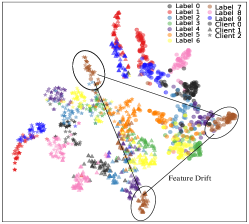
(a) FedAvg without VHL

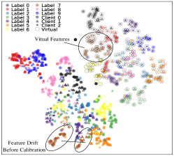
(b) FedAvg with Naive VHL

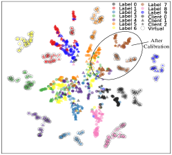
(c) FedAvg with VHL

Figure 2: The t-SNE Visualization of empirical feature distribution of 3 different clients training with FedAvg, at $299$-th communication round. Different colors represent different classes of data, different shapes represent different clients, and the dotted circle means the virtual data. The Naive VHL means training with both the private natural and shared virtual data without feature calibration.

4 Related Work

We merely introduce the most related works in this section due to the limited space and leave more detailed discussion and literature review in Appendix B.

Mitigating Client Drift. A series of works focus on adding regularization to calibrate the optimization direction of local models, restricting local models from being too far away from the server model, including FedProx (Li et al., 2020a), FedDyn (Acar et al., 2021), SCAFFOLD (Karimireddy et al., 2020), MOON (Li et al., 2021b), and FedIR (Hsu et al., 2020). From the optimization point of view, some methods propose to correct the updates from clients, accelerating and stabilizing the convergence, like FedNova (Wang et al., 2020), FedAvgM (Hsu et al., 2019), FedAdaGrad, FedYogi, and FedAdam (Reddi et al., 2021).

Sharing Data. Some works propose to utilize GANs (Jeong et al., 2018; Long et al., 2021) or adversarial learning (Goetz & Tewari, 2020) to generate synthetic data based on the information of the raw data. Nonetheless, all above methods could expose the information of the raw data at some degree, i.e. intermediate features, statistic information, raw data.

The statistical information of the raw data (Yoon et al., 2021; Shin et al., 2020) is also employed to learn and share synthetic data. The profiles of the raw images could be still seen from the synthetic images, exposing the raw data information at a degree. Thus, the intermedia activations (Hao et al., 2021) or logits (Li & Wang, 2019; Chang et al., 2019; Luo et al., 2021) of the raw data are exploited to enhance FL. However, these methods may expose the accurate high-level semantic information of raw data, making clients under the risks of exposing the private data. Specifically, the raw data may be reconstructed by feature inversion methods (Zhao et al., 2021). Table 7 in Appendix B summarizes these sharing data approach, but we omitted the comparison with works because of the above privacy concerns .

5 Experimental Studies

5.1 Experiment Setup

Federated Datasets and Models. To verify the effectiveness of VHL, we exploit a popular FedML framework (He et al., 2020) to conduct experiments over various datasets including CIFAR-10 (Krizhevsky & Hinton, 2009), FMNIST (Xiao et al., 2017), SVHN (Netzer et al., 2011), and CIFAR-100 (Krizhevsky & Hinton, 2009). We use ResNet-18 (He et al., 2016) for CIFAR-10, FMNIST and SVHN, and ResNet-50 for CIFAR-100. To emulate data distribution in FL, we partition the datasets with a commonly used Non-IID partition method, Latent Dirichlet Sampling (Hsu et al., 2019). Following existing works (Li et al., 2021b; Luo et al., 2021), each dataset is partitioned with two different Non-IID degrees using $a=0.1$ and $a=0.05$.

Moreover, to verify the effect of VHL on other kinds of Non-IID data distributions, we conduct experiments on CIFAR-10 with 10 clients using another two kinds of Non-IID partition methods: (1) 2-classes partition (McMahan et al., 2017): each client only has 500 data samples of 2 classes; (2) subset partition (Zhao et al., 2018): all clients have data of all 10 classes, but each client has one dominant class with 4950 samples, and each of the remaining classes has 5 or 6 samples, which is an extremely imbalanced distribution.

Baselines. We conduct FedAvg (McMahan et al., 2017) and recent effective FL algorithms that are proposed to address the client drift problem, including FedProx (Li et al., 2020a), SCAFFOLD (Karimireddy et al., 2020), and FedNova (Wang et al., 2020), with or without VHL. The detailed hyper-parameters of each algorithm in each setting are reported in Appendix C.

Generating Virtual Datasets. We use an un-pretrained StyleGAN-v2 (Karras et al., 2020) without using any training data to generate the virtual dataset. Specifically, the server uses the StyleGAN to generate images with different latent styles and noises which are sampled from different Gaussian Distributions. We show these virual noise in Figure 4 and  5 in Appendix C.3. The generated virtual images are then distributed to all clients at the beginning of training. We also explore other methods (i.e., generated with a simple generative model and up-sampling with pure Gaussian noises) to generate virtual datasets in section 5.4. More generation details of virtual datasets are listed in Appendix C.3.

Table 1: Results with/without VHL on CIFAR-10.

	ACC $\uparrow$	ROUND $\downarrow$	Speedup $\uparrow$
	w/ (w/o) VHL
centralized training ACC = 92.88% (92.53%)
$a=0.1,E=1,K=10$ ( Target ACC = 79% )
FedAvg	87.82 (79.98)	128 (287)	$\times$ 2.2 ($\times$ 1.0)
FedProx	87.30 (83.56)	128 (188)	$\times$ 2.2 ($\times$ 1.5)
SCAFFOLD	84.87 (83.58)	90 (291)	$\times$3.2 ($\times$ 1.0)
FedNova	87.56 (81.35)	128 (351)	$\times$ 2.2 ($\times$ 0.8)
$a=0.05,E=1,K=10$ ( Target ACC = 69% )
FedAvg	79.23 (69.02)	112 ( 411 )	$\times$ 3.7 ($\times$ 1.0)
FedProx	80.84 (78.66)	151 ( 201 )	$\times$ 2.7 ($\times$ 2.0)
SCAFFOLD	55.73 (38.55)	Nan (Nan)	Nan (Nan)
FedNova	80.59 (64.78)	247 (Nan)	$\times$ 1.66 (Nan)
$a=0.1,E=5,K=10$ ( Target ACC = 84% )
FedAvg	89.93 (84.79)	91 (255 )	$\times$ 2.8 ($\times$ 1.0)
FedProx	86.41 (82,18)	255 (Nan)	$\times$ 1.0 (Nan)
SCAFFOLD	87.27 (86.20)	45 (66)	$\times$ 5.7 ($\times$ 2.0)
FedNova	90.24 (86.09)	67 (127)	$\times$ 3.8 ($\times$ 1.0)
$a=0.1,E=1,K=100$ ( Target ACC = 49% )
FedAvg	70.20 (49.61)	385 (957)	$\times$ 2.5 ($\times$ 1.0)
FedProx	73.90 (49.97)	325 (842)	$\times$ 2.9 ($\times$ 1.1)
SCAFFOLD	59.66 (52.24)	479 (664)	$\times$ 2.0 ($\times$ 1.4)
FedNova	61.59 (46.53)	554 (Nan)	$\times$ 1.7 (Nan)

• “ROUND” represents the communication rounds that need to attain the target accuracy. The notion $\downarrow$ ($\uparrow$) indicates smaller (larger) values are preferred. “Nan” means that the target accuracy is never attained during the whole training process.

Table 2: Results with/without VHL on FMNIST.

	ACC $\uparrow$	ROUND $\downarrow$	Speedup $\uparrow$
	w/ (w/o) VHL
centralized training ACC = 93.80% (93.70%)
$a=0.1,E=1,K=10$ ( Target ACC = 86% )
FedAvg	92.05 (86.81)	52 (119)	$\times$ 2.3 ($\times$ 1.0)
FedProx	90.68 (87.12)	31 (135)	$\times$ 3.8 ($\times$ 0.9)
SCAFFOLD	90.27 (86.21)	14 (143)	$\times$ 8.5 ($\times$ 0.8)
FedNova	91.88 (86.99)	52 (83)	$\times$ 2.3 ($\times$ 1.4)
$a=0.05,E=1,K=10$ ( Target ACC = 78% )
FedAvg	89.06 (78.57)	53 (425)	$\times$ 8.0 ($\times$ 1.0)
FedProx	87.76 (81.96)	30 (41)	$\times$ 14.2 ($\times$ 10.4)
SCAFFOLD	80.68 (76.08)	58 (Nan)	$\times$ 7.3 (Nan)
FedNova	87.25 (79.06)	30 (538)	$\times$ 14.2 ($\times$ 0.8)
$a=0.1,E=5,K=10$ ( Target ACC = 87% )
FedAvg	91.52 (87.45)	51 (278)	$\times$ 5.5 ($\times$ 1.0 )
FedProx	88.27 (86.07)	74 (Nan)	$\times$ 3.8 (Nan)
SCAFFOLD	91.82 (87.10)	20 (105)	$\times$ 13.9 ($\times$ 2.7)
FedNova	91.86 (87.53)	51 (193)	$\times$ 5.5 ($\times$ 1.4)
$a=0.1,E=1,K=100$ ( Target ACC = 90% )
FedAvg	91.14 (90.11)	436 (658)	$\times$ 1.5 ($\times$ 1.0)
FedProx	91.37 (90.71)	283 (491)	$\times$ 2.3 ($\times$ 1.3)
SCAFFOLD	87.91 (85.99)	Nan (Nan)	Nan (Nan)
FedNova	88.34 (87.09)	Nan (Nan)	Nan (Nan)

5.2 Experimental Results

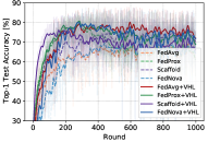
(a) Test Accuracy

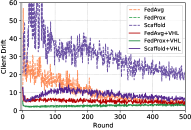
(b) Model Divergence

Figure 3: CIFAR10 with $a=0.1$, $E=1$, $K=10$. Grey lines represent the test accuracy, and solid lines represents smoothed version of the grey lines for better visualization.

Main Results. We use two metrics, the best accuracy during training and the number of communication rounds to achieve target accuracy, to compare the performance of different algorithms. The target accuracy is set as the best accuracy of FedAvg. The results on CIFAR-10, FMNIST, SVHN, and CIFAR-100 are shown in Tables 1,  2,  4, and  5, respectively. We also compare the convergence speed in Figure  3 (a) on CIFAR-10. The results show that VHL not only improves the generalization ability, but also accelerates the convergence. We also measure the client drift (Karimireddy et al., 2020), $\frac{1}{|\mathcal{S}^{r}|}\sum_{i\in\mathcal{S}^{r}}\|\bar{w}-w_{i}\|$, in Figure 3 (b), where we report the client drift for the first 500 rounds as the early stage of training has obvious client drift problems. Note that we exclude FedNova from comparison as its client drift is very severe. The Figure 3 (b) show that VHL could greatly alleviate client drift, thus accelerating convergence.

Impacts of Non-IID Degree. As shown in Tables 1, 2, 4, and 5, for all datasets with high Non-IID degree ($a=0.05$), the VHL gains more performance improvement than the case of lower Non-IID degree ($a=0.1$), which verifies that VHL could effectively defend against data heterogeneity.

Different Non-IID Partition Methods. The experiment results of another two kinds of Non-IID partition methods are listed in Table 3. Compared with LDA parition with $a=0.1$, these two kinds of Non-IID distribution make the generalization performance of FL drops much more. For these more difficult tasks, VHL gains much more performance improvement than other algorithms, which demonstrates that VHL could well defend different kinds of data heterogeneity.

Table 3: Experiment results of other Non-IID partition methods.

	Test Accuracy w/(w/o) VHL
Partition	FedAvg	FedProx	SCAFFOLD	FedNova
2-classes	71.88/41.74	75.43/54.21	66.02/46.67	73.46/43.38
Subset	50.29/38.33	39.41/33.66	43.77/33.35	38.22/32.18

Different Number of Clients. The 10-client setting simulates the cross-silo FL in which clients have larger dataset, and the 100-client setting simulates cross-device FL in which clients have smaller dataset. As shown in Tables 1, 2, 4, and 5, VHL boosts the generalization performance and significantly reduces the communication cost to achieve the target accuracy in both scenarios.

Different Local Epochs. Results in Tables 1, 2, 4, and 5 show that when increasing local training epochs, VHL also benefits FL. However, as shown in Table 5, for CIFAR-100 when $E=5$, VHL does not work well. We suppose that reasons exist in two aspects: 1) As shown in Table 5, the test accuracy of centralized training using VHL is worse than the normal training. The larger number of classes need larger model capacity. The ResNet-50 cannot attain a high test accuracy on CIFAR-100, not to say 200 classes with the virtual dataset. 2) The larger local epochs means that clients will train more local iterations, which may cause clients to have a drifted feature expression of the virtual data, leading to the failure of calibration.

Visualization of Feature Distribution. To understand how VHL helps generalize the model, we exploit t-SNE (van der Maaten & Hinton, 2008) to show the feature distributions of clients at the $299$-th communication round. To highlight the generalization performance, we show the features on test datasets, where merely 3 clients are used considering the better visualization. And we also report feature distributions at different communication rounds in Appendix D.1. in Figure 2. From Figure 2 (a), we can see that FedAvg makes most features from different labels at the same client be very close, and it makes the features from the same class be separate. It indicates that different clients have very different feature representation for the same or similar inputs in FedAvg, which results in poor generalization ability of the trained model. As shown in Figure 2 (b), after local training with the virtual data without feature calibration (called Naive VHL), we can see the features of virtual data are consistent in all clients as the virtual data is shared, but the feature distributions of the original data are only slightly better than the naive FedAvg. Thus, we would like to pull the features of the original dataset close to the virtual dataset so that the corrected training data has a relatively low data heterogeneity. As shown in Figure 2 (c), after we applied the feature calibration in VHL, the features from the same class at different clients are gathered closely and become compact. It indicates that training with VHL can help different clients learn homogeneous natural features for the same classes.

Table 4: Results with/without VHL on SVHN.

	ACC $\uparrow$	ROUND $\downarrow$	Speedup $\uparrow$
	w/ (w/o) VHL
centralized training ACC = 95.01% (95.27%)
$a=0.1,E=1,K=10$ ( Target ACC = 88% )
FedAvg	93.49 (88.56)	75 (251)	$\times$ 3.3 ($\times$ 1.0)
FedProx	91.70 (86.51)	271 (Nan)	$\times$ 0.9 (Nan)
SCAFFOLD	87.54 (80.61)	Nan (Nan)	Nan (Nan)
FedNova	93.35 (89.12)	75 (251)	$\times$ 3.3 ($\times$ 1.0)
$a=0.05,E=1,K=10$ ( Target ACC = 82% )
FedAvg	92.26 (82.67)	94 (357)	$\times$ 3.8 ($\times$ 1.0)
FedProx	89.30 (78.57)	320 (Nan)	$\times$ 1.1 (Nan)
SCAFFOLD	83.89 (74.23)	147 (Nan)	$\times$ 2.4 (Nan)
FedNova	91.82 (82.22)	128 (741)	$\times$ 2.8 ($\times$ 0.5)
$a=0.1,E=5,K=10$ ( Target ACC = 87% )
FedAvg	90.52 (87.92)	145 (131)	$\times$ 0.9 ($\times$ 1.0)
FedProx	87.20 (78.43)	351 (Nan)	$\times$ 0.4 (Nan)
SCAFFOLD	88.04 (81.07)	210 (Nan)	$\times$ 0.6 (Nan)
FedNova	90.99 (88.17)	75 (162)	$\times$ 1.7 ($\times$ 0.8)
$a=0.1,E=1,K=100$ ( Target ACC = 89% )
FedAvg	92.05 (89.44)	362 (618)	$\times$ 1.7 ($\times$ 1.0)
FedProx	92.08 (89.51)	356 (618)	$\times$ 1.7 ($\times$ 1.0)
SCAFFOLD	89.21 (89.55)	968 (643)	$\times$ 0.6 ( $\times$ 1.0 )
FedNova	92.01 (82.08)	676 (Nan)	$\times$ 0.9 (Nan)

Table 5: Results with/without VHL on CIFAR-100.

	ACC $\uparrow$	ROUND $\downarrow$	Speedup $\uparrow$
	w/ (w/o) VHL
centralized training ACC = 71.90 % (74.25 %)
$a=0.1,E=1,K=10$ ( Target ACC = 67% )
FedAvg	70.04 (67.95)	384 (497)	$\times$ 1.3 ($\times$ 1.0)
FedProx	68.29 (65.29)	617 (Nan)	$\times$ 0.8 (Nan)
SCAFFOLD	67.88 (67.14)	294 (766)	$\times$ 1.7 ($\times$ 0.6)
FedNova	69.58 (68.26)	384 (472)	$\times$ 1.3 ($\times$ 1.1)
$a=0.05,E=1,K=10$ ( Target ACC = 62% )
FedAvg	65.61 (62.07)	354 (514)	$\times$ 1.5 ($\times$ 1.0)
FedProx	64.39 (61.52)	482 (Nan)	$\times$ 1.1 (Nan)
SCAFFOLD	60.67 (59.04)	Nan (Nan)	Nan (Nan)
FedNova	66.45 (60.35)	320 (Nan)	$\times$ 1.6 (Nan)
$a=0.1,E=5,K=10$ ( Target ACC = 69% )
FedAvg	69.85 (69.81)	327 (283)	$\times$ 0.9 ($\times$ 1.0)
FedProx	63.83 (62.62)	Nan (Nan)	Nan (Nan)
SCAFFOLD	69.43 (70.68)	291 (171)	$\times$ 1.0 ($\times$ 1.7)
FedNova	68.86 (70.05)	Nan (292)	Nan ($\times$ 1.0)
$a=0.1,E=1,K=100$ ( Target ACC = 48% )
FedAvg	53.45 (48.33)	717 (967)	$\times$ 1.3 ($\times$ 1.0)
FedProx	52.68 (48.14)	717 (955)	$\times$ 1.3 ($\times$ 1.0)
SCAFFOLD	54.93 (51.63)	656 (827)	$\times$ 1.5 ($\times$ 1.2)
FedNova	53.50 (48.12)	797 (967)	$\times$ 1.2 ($\times$ 1.0)

5.3 Other Facets of VHL

In this section, we dive into VHL deeper by further studying other facets related to it. In addition, we conduct experiments on CIFAR to investigate the intriguing property of VHL. All of these experimental results are listed in Table 6.

Transfer Learning from Virtual Dataset. The deep learning model pretrained on virtual datasets could also perform well on realistic datasets (Baradad et al., 2021). Thus, to understand whether the benefits of VHL come from only conducting transfer learning from the virtual dataset, we pretrain the server model with the virtual dataset, and then conduct vanilla FedAvg. We call this simple algorithm as virtual federated transfer learning (VFTL). The results of this experiment are shown in Table 6. Due to the limited space, we show the convergence curve of this experiment in the Figure 18 (a) in Appendix D.2. The experimental results show that the model performance could not benefit from such a pretraining on virtual dataset. But the Figure 18 (a) shows the VFTL could provide some convergence speedup at the beginning of training. We suppose such an initial speedup comes from the better feature extractor of the pretrained model. This phenomenon is compatible with the recently finding that the loading pretrained model could accelerate FL training (He et al., 2021).

Naive VHL. We study the effect of simply training with the natural data together with the virtual dataset, without any extra algorithm designs. In this experiment, clients will sample both natural data together with the virtual data, without feature calibration.

The experiment results are listed in Table 6, showing that even simply adding the virtual dataset could also benefit FL. We conjecture that the benefit of this may come from several aspects: 1) As the data heterogeneity decreases, the client drift is alleviated; 2) The client models could learn low-level features from the virtual data, thus there exists the effect of transfer learning from the virtual dataset; 3) By adding the virtual dataset, the clients now have more classes than before, which can effectively alleviate the negative impact of local dominant classes on classifiers, which is also studied by (Luo et al., 2021; Yu et al., 2021).

Virtual Feature Alignment. To validate the effect of feature calibration, we completely eliminate the effect of the virtual data by removing the virtual dataset, and sampling new features from different Gaussian distributions. Then, we conduct feature calibration based on these shared features. We name this simple method as Virtual Feature Alignment (VFA). Besides aligning the features, we can also employ approaches like style normalization (Jin et al., 2020) to mitigate the domain gap. As shown in Table 6, feature calibration benefits FL even only with the random features. Although the performance of VFA falls behind the VHL, it is valuable to explore VFA, due to its computation efficiency.

Table 6: Experiment results of further study of VHL on CIFAR10.

	FedAvg	FedProx	SCAF.	FedNova
Baselines	79.98	83.56	83.58	81.35
VHL	87.82	87.30	84.87	87.56
Other Facets of VHL
VFTL	80.38	82.20	83.83	80.63
Naive VHL	86.50	85.66	85.70	85.74
VFA	85.14	84.75	85.31	86.59
Ablation Study
Pure Noise	87.01	86.46	85.57	87.81
Simple-CNN	84.87	85.30	84.15	85.25
Tiny-ImageNet	84.05	83.62	81.57	85.41
$B_{v}=64$	87.36	86.36	82.39	87.20
$B_{v}=128$	87.82	87.30	84.87	87.56
$B_{v}=256$	88.95	86.82	84.68	87.89
$B_{v}=384$	89.69	86.59	85.87	88.73
$\lambda=0.1$	87.02	86.12	84.25	87.02
$\lambda=0.2$	87.04	86.02	84.41	87.65
$\lambda=0.5$	87.02	85.99	84.29	87.15
$\lambda=1.0$	87.82	87.30	84.87	87.56
$\lambda=2.0$	87.87	86.86	84.81	88.71
$\lambda=5.0$	83.52	88.34	85.58	88.47
$\lambda=10.0$	88.65	88.41	85.29	88.39
$h_{shallow}$	86.10	85.59	85.19	84.95
$h_{middle}$	87.06	86.30	87.97	87.27
$h_{deep}$	89.26	87.54	86.00	88.42
$h_{last}$	87.82	87.30	84.87	87.56
Model Capacity
Res10-Baselines	83.55	82.76	82.91	83.14
Res10-VHL	87.39	86.08	85.09	88.03
Res18-Baselines	79.98	83.56	83.58	81.35
Res18-VHL	87.82	87.30	84.87	87.56
Res34-Baselines	82.73	84.04	81.11	82.48
Res34-VHL	87.92	88.05	84.80	88.74

5.4 Ablation Study

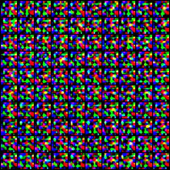
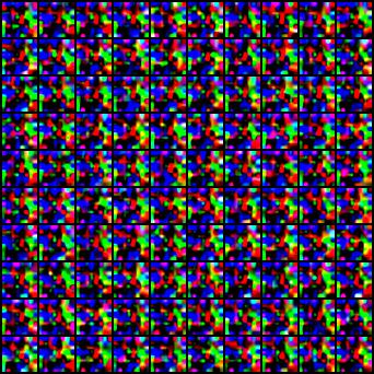
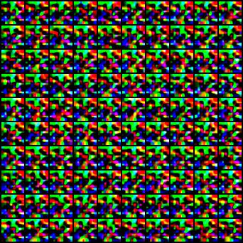
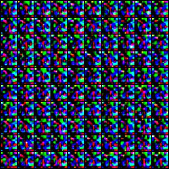
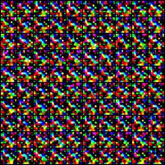
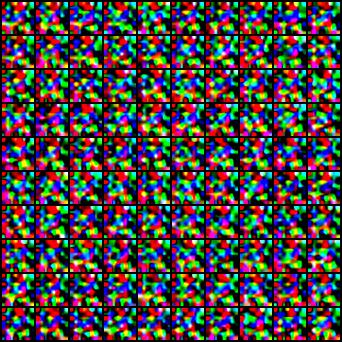
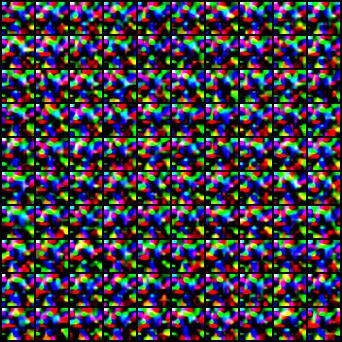
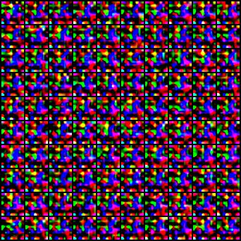
Figure 6: Generated Gaussian Noise with upsampling.

VHL with Other Datasets. We study the effect of replacing the virtual dataset generated by the StyleGAN to other datasets. The first dataset is generated by upsampling the pure Gaussian Noise, which is shown in Figure 6 in the Appendix C.3. The second dataset is generated by a simple CNN rather than StyleGAN shown in Figure 7 in the Appendix C.3. And the third dataset is a 10-class subset of Tiny-ImageNet (Le & Yang, 2015).

As shown in Table 6, VHL with the simple pure noise could benefit FL, reducing the difficulty of generating the virtual dataset. And it shows that using a Tiny-ImageNet as our virtual dataset could not outperform using pure noise, which is a bit surprising. Because the realistic dataset may have more plentiful semantic information than the virtual dataset. The possible reason is that, the Tiny-ImageNet is more difficult to be separated than the generated virtual dataset, thus the feature calibration cannot work well. To verify this hypothesis, We report the curve of the training accuracy on the virtual dataset in Figure 18 (c) in Appendix D.2.

Sampling More Virtual Data. We note that under the high Non-IID degree, some clients would own much more data samples than the virtual data, reducing the effect of feature calibration. Therefore, we consider increasing the sampling weight of the virtual data, making clients to see more virtual data to strengthen the effect of calibration. We conduct VHL with CIFAR-10 with different batch size $B_{v}$ to verify the effect of sampling more virtual data. The experiment results are shown in Table 6 and Figure 18 (a) in Appendix D.2, demonstrating that sampling more virtual data could strengthen the effect of VHL.

Different Calibration Weight. We adjust different calibration weights $\lambda$ as sensitivity test. The experimental results are listed in Table 6, showing that VHL is not sensitive to the calibration weight.

Using Features of Different Layers. To study the impact of features from different layers, we conduct calibration based on different output layers of ResNet-18. We find that using the features from the $4$-th layer of ResNet-18 has the best performance. We suppose that calibration based on too shallow layer may be not enough to impact the subsequent layers feature shift. However, the calibration based on the last layer may interrupt the normal classification between the natural data and the virtual data, because which have completely different high-level semantic information.

Model Capacity. Adding more data means deep learning models may need more model capacity, so we investigate the sensitivity of VHL to model capacity. We conduct experiments on CIFAR-10 with different models, including ResNet-10, ResNet-18 and ResNet-34. Results in Table 6 show that VHL could perform well on all three models of different model capacity.

5.5 Limitations

Guarantee the Diversity of the Virtual Dataset. In our method, the virtual dataset needs the same number of classes as the original datasets, so that the label alignment could be implemented. However, when meeting numerous classes of original datasets, generating a virtual dataset with enough diversity may cost more calculation resources.

Extra Calculation. VHL needs to conduct training on the virtual data, causing the extra calculation cost. VFA is a possible direction to reduce the calculation, as mentioned in Sec. 5.3. We compare the calculation cost of different algorithms in Table 10 in Appendix D.3.

6 Conclusion

In this paper, we find that FL could remarkably benefit from a virtual dataset containing no information related to the natural dataset, shedding light on the data heterogeneity mitigation from a virtual data perspective. Through the calibration on the homogeneous virtual data, FL could attain significant performance improvement and much less client drift. Our contribution not only exists in the improvements of model performance in FL, but also in inspiring a new viewpoint to FL with many intriguing experimental phenomena. We hope the future works could unearth more things about VHL and exploit it to enhance FL or other machine learning tasks.

Appendix A Proof

A.1 Proof of Theorem 3.2

Recall that the model $f$ can be decomposed as $f=\phi\circ\rho$, the statistical margin for $f$ then becomes:

$$\textit{SM}_{m}(f,\mathcal{P}(x,y))=\textit{SM}_{m}(\rho,\mathcal{P}(\phi(x),y)).$$ (6)

In what follows, we use $\mathcal{P}(\phi,y)$ to represent $\mathcal{P}(\phi(x),y)$ for brevity.

Before giving detailed proof, we introduce a lemma:

Lemma A.1.

Let $\mathcal{P}$ and $\mathcal{P}_{v}$ be two distributions with identical label distributions, $d\left(\cdot,\cdot\right)$ be the Wasserstein distance of two distributions, i.e.,

$$d\left(\mathcal{P}\left(\phi|y\right),\mathcal{P}_{v}\left(\phi|y\right)\right)=\inf_{J\in\mathcal{J}(\mathcal{P}(\phi|y),\mathcal{P}_{v}(\phi|y))}\mathbb{E}_{(\phi,\phi^{\prime})\sim J}\ m(\phi,\phi^{\prime}),$$

where $\mathcal{J}(\mathcal{P}(\phi|y),\mathcal{P}_{v}(\phi|y))$ is the set of joint distributions of $\mathcal{P}(\phi|y)$ and $\mathcal{P}_{v}(\phi|y)$. Then, we have

$$\mathbb{E}_{y}d(\mathcal{P}(\phi|y),\mathcal{P}_{v}(\phi|y))\geq|\mathbb{E}_{\rho:=\textit{VHL}(\mathcal{P}_{v}(\phi,y))}[\textit{SM}_{m}(\rho,\mathcal{P}(\phi,y))-\textit{SM}_{m}(\rho,\mathcal{P}_{v}(\phi,y))]|.$$

Proof.

We construct an optimal transport $\mathcal{J}^{*}_{y}$ between the conditional distributions $\mathcal{P}|y$ and $\mathcal{P}_{v}|y$. Using the auxiliary distribution, we have

$$\begin{split}\textit{SM}_{m}(\rho,\mathcal{P}(\phi,y))&=\mathbb{E}_{(\phi,y)\sim\mathcal{P}}\inf_{\rho(\phi^{\prime})\neq y}m(\phi^{\prime},\phi)=\mathbb{E}_{y}\mathbb{E}_{\phi\sim\mathcal{P}|y}\inf_{\rho(\phi^{\prime})\neq y}m(\phi^{\prime},\phi)=\mathbb{E}_{y}\mathbb{E}_{(\phi,\phi^{\prime\prime})\sim\mathcal{J}^{*}_{y}}\inf_{\rho(\phi^{\prime})\neq y}m(\phi^{\prime},\phi)\\ &\leq\mathbb{E}_{y}\mathbb{E}_{(\phi,\phi^{\prime\prime})\sim\mathcal{J}^{*}_{y}}\inf_{\rho(\phi^{\prime})\neq y}[m(\phi^{\prime},\phi^{\prime\prime})+m(\phi^{\prime\prime},\phi)]\\ &=\mathbb{E}_{y}\mathbb{E}_{(\phi,\phi^{\prime\prime})\sim\mathcal{J}^{*}_{y}}\inf_{\rho(\phi^{\prime})\neq y}m(\phi^{\prime\prime},\phi^{\prime})+\mathbb{E}_{y}\mathbb{E}_{(\phi,\phi^{\prime\prime})\sim\mathcal{J}^{*}_{y}}m(\phi^{\prime\prime},\phi)\\ &=\mathbb{E}_{(\phi^{\prime\prime},y)\sim\mathcal{P}_{v}}\inf_{\rho(\phi^{\prime})\neq y}m(\phi^{\prime\prime},\phi^{\prime})+\mathbb{E}_{y}d(\mathcal{P}(\phi|y),\mathcal{P}_{v}(\phi|y))\\ &=\textit{SM}_{m}(\rho,\mathcal{P}_{v}(\phi,y))+\mathbb{E}_{y}d(\mathcal{P}(\phi|y),\mathcal{P}_{v}(\phi|y)).\end{split}$$ (7)

Similarly, we have

$$\textit{SM}_{m}(\rho,\mathcal{P}_{v}(\phi,y))\leq\textit{SM}_{m}(\rho,\mathcal{P}(\phi,y))+\mathbb{E}_{y}d(\mathcal{P}(\phi|y),\mathcal{P}_{v}(\phi|y)).$$ (8)

Combining Eq. 7 and Eq. 8, we have

$$\mathbb{E}_{y}d(\mathcal{P}(\phi|y),\mathcal{P}_{v}(\phi|y))\geq|\mathbb{E}_{\rho:=\textit{VHL}(\mathcal{P}_{v}(\phi,y))}[\textit{SM}_{m}(\rho,\mathcal{P}(\phi,y))-\textit{SM}_{m}(\rho,\mathcal{P}_{v}(\phi,y))]|.$$ (9)

This completes the proof. ∎

In addition, we decompose $\textit{SM}_{m}(f,\mathcal{P}(\phi,y))$ as follows:

$$\textit{SM}_{m}(f,\mathcal{P}(\phi,y))=\textit{SM}_{m}(f,\mathcal{P}(\phi,y))-\textit{SM}_{m}(f,\mathcal{P}_{v}(\phi,y))+\textit{SM}_{m}(f,\mathcal{P}_{v}(\phi,y))-\textit{SM}_{m}(f,\tilde{D}(\phi,y))+\textit{SM}_{m}(f,\tilde{D}(\phi,y)),$$

where $\tilde{D}(\phi,y)$ stands for the training set containing $n_{v}$ samples drawn from $\mathcal{P}_{v}(\phi,y)$. In what follows, we omit $(\phi,y)$ for each joint distribution, e.g., using $\mathcal{P}$ for $\mathcal{P}(\phi,y)$, and denote $\mathbb{E}_{\rho:=\textit{VHL}(\mathcal{P}(\phi,y))}$ as $\mathbb{E}_{\rho\leftarrow\mathcal{P}}$ for brevity.

Theorem A.2.

Let $f=\phi\circ\rho$ be a neural network decompose of a feature extractor $\phi$ and a classifier $\rho$, $\mathcal{P}(x,y)$ and $\mathcal{P}_{v}(x,y)$ are natural and virtual distributions with identical label distributions. Then, learning $f$ with the proposed distribution mismatch penalty, i.e., Eq. 4 elicits an model with bounded statistical margin, i.e., Definition 3.1.

Proof.

Built upon the decomposition and lemma A.1, we can bound the statistical margin $\mathbb{E}_{\rho\leftarrow\mathcal{P}_{v}}\textit{SM}_{m}(\rho,\mathcal{P})$:

$$\begin{split}\mathbb{E}_{\rho\leftarrow\mathcal{P}_{v}}\textit{SM}_{m}(\rho,\mathcal{P})&\geq\mathbb{E}_{\rho\leftarrow\mathcal{P}_{v}}\textit{SM}_{m}(\rho,\tilde{D})-|\mathbb{E}_{\rho\leftarrow\mathcal{P}_{v}}[\textit{SM}_{m}(\rho,\mathcal{P}_{v})-\textit{SM}_{m}(\rho,\tilde{D})]|-|\mathbb{E}_{\rho\leftarrow\mathcal{P}_{v}}[\textit{SM}_{m}(\rho,\mathcal{P})-\textit{SM}_{m}(\rho,\mathcal{P}_{v})]|\\ &\geq\mathbb{E}_{\rho\leftarrow\mathcal{P}_{v}}\textit{SM}_{m}(\rho,\tilde{D})-|\mathbb{E}_{\rho\leftarrow\mathcal{P}_{v}}[\textit{SM}_{m}(\rho,\mathcal{P}_{v})-\textit{SM}_{m}(\rho,\tilde{D})]|-\mathbb{E}_{y}d(\mathcal{P}(\phi|y),\mathcal{P}_{v}(\phi|y))\end{split}$$ (10)

The first and second term $\mathbb{E}_{\rho\leftarrow\mathcal{P}_{v}}\textit{SM}_{m}(\rho,\tilde{D}),|\mathbb{E}_{\rho\leftarrow\mathcal{P}_{v}}[\textit{SM}_{m}(\rho,\mathcal{P}_{v})-\textit{SM}_{m}(\rho,\tilde{D})]|$ can be bounded by maximizing the statistical margin (Diochnos et al., 2018), requiring that the distribution $\mathcal{P}_{v}$ is separable. Specifically, the first term reveals that the statistical margin on the training set should be large, and the second term further requires that the statistical margin should be large on the (virtual) distribution. The last term $\mathbb{E}_{y}d(\mathcal{P}(\phi|y),\mathcal{P}_{v}(\phi|y))$ is bounded by the conditional distribution, i.e., Eq 4. Hence, the statistical margin elicited by Eq. 4 is bounded, leading to bounded generalization performance. ∎

Appendix B More Related work

B.1 Federated Learning

Federated Learning (FL) is first proposed by (McMahan et al., 2017) as a distributed algorithm to protect users’ data privacy while collaboratively training a global model. The heterogeneous data distribution across all clients severely damage the convergence of federated learning and final performance (Zhao et al., 2018; Li et al., 2020b; Kairouz et al., 2021; Tang et al., 2021). When training with the heterogeneous data, local and global models are much more unstable than centralized training (Karimireddy et al., 2020). And there exists a more severe divergence between local models of FL than that of distributed training with IID data (Li et al., 2020a; Karimireddy et al., 2020). This inconsistency is called client drift.

To mitigate the client drift, hyper-parameters may need to be carefully adjusted (Wang et al., 2021), like learning rate and local training iterations, which directly decide how fast local model move and thus how far drift they could be. However, too small learning rate also means slower convergence. Thus, how to simultaneously achieve faster training speed and a more gentle client drift is important. To this end, many research works try to design more effective federated learning algorithms to address client drift problem.

Model Regularization. This line of research focus on adding regularization to calibrate the optimization direction of local models, restricting local models from being too far away from the server model. FedProx (Li et al., 2020a) adds a penalty of the L2 distance between local models to the server model.

SCAFFOLD (Karimireddy et al., 2020) utilizes the history information to reduce the “client variance”, thus decreasing the client drift. MOON (Li et al., 2021b) performs contrastive learning between the server model and client models, calibrating clients’ learned representation.

Optimization Schemes. From the optimization point of view, some methods propose to correct the updates from clients, accelerating and stabilizing the convergence. FedNova  (Wang et al., 2020) propose to normalize the local updates to eliminate the inconsistency between the local and global optimization objective functions.  (Hsu et al., 2019) proposes FedAvgM, which exploits the history updates of server model to avoid the overfits on the selected clients at current round. A recent work (Reddi et al., 2021) proposes FEDOPT, which generalizes the centralized optimization methods into FL scenario, like FedAdaGrad, FedYogi, FedAdam.

Sharing Data. Because the original cause of client drift is the data heterogeneity, another line of research focuses on generating more data that carries some information of the natural data, and sharing them to all clients. It has been found that sharing a part of natural data could significantly benefit federated learning (Zhao et al., 2018), yet which sacrifices the privacy of clients’ data.

A series of works (Hardt & Rothblum, 2010; Hardt et al., 2012; Chatalic et al., 2021; Johnson et al., 2018; Cai et al., 2021) add noise on data queries to implement sharing data with privacy guarantee at some degree. In addition, sharing incomplete data is also a promising direction, where the generation process can be similar to  (Yang et al., 2021).

FD (Jeong et al., 2018) proposes to let clients collectively train a generative model to locally reproduce the data samples of all devices, augmenting their local data to become IID. G-PATE (Long et al., 2021) leverages GAN to generate data, with private aggregation among different discriminators to ensure privacy guarantees at some degree.  (Goetz & Tewari, 2020) utilized the adversarial learning to generate data samples based on the raw data to help FL.

Fed-ZDAC (Hao et al., 2021) utilize the intermedia activations and BN layer statistic of the raw data information to learn and share synthetic data. The profiles of the raw images could be still seen from the synthetic images, exposing the raw data information at a degree. XorMixFL (Shin et al., 2020) proposes to collect other clients’ XOR-encoded data samples that are decoded only using each client’s own data samples, also exposing raw data information to other clients. FedMIX (Yoon et al., 2021) proposes to let clients send and receive the averaged local data of each batch. Strictly speaking, this method exposes the statistic information of local data, i.e. the mean values.

FedMD (Li & Wang, 2019), Cronus (Chang et al., 2019) and CCVR (Luo et al., 2021) transmit the logits information of data samples to enhance FL, which may expose the accurate high-level semantic information of raw data.

FedDF (Lin et al., 2020) utilizes other data and conduct knowledge distillation based on these data, to transfer knowledge of models between server and clients. The most difference between FedDF and VHL is that our model will be directly trained on the virtual data, which is seen as a part of the new objective function. And VHL does not require the shared dataset to be meaningful and has transferability with raw data.

To highlight our novelty, we compare and demystify different FL algorithms related to the sharing data in Table 7. We would like to clarify that we are the first to raise and analyze the question of how to introduce virtual datasets (even pure noise) containing absolutely no private information to promote FL. Specifically, related works, i.e., the first 9 lines in Table 7, have risks of exposing private data, while the 10-th related work in Table 7, FedDF, requires a distribution similar to the private distribution, see Theorem 5.1 in the FedDF. In contrast, we consider arbitrary datasets with no private information.

We omitted the comparison with works in Table 7, because of the above differences. Because FedDF does not expose the information of the raw data, we compare VHL with the FedDF. We have conducted experiments using the same settings as in FedDF. The results are listed in Table 8. For FedDF, the distribution similar to the private distribution (FedDF + real) improves the accuracy, while noise (FedDF + noise) degrades the accuracy. VHL could perform much better with the noise dataset.

Table 7: Demystifying different FL algorithms related to the sharing data.

	Shared Data	Relation with Private Raw Data	Objective of the Algorithm
FD (Jeong et al., 2018)	Sythetic Data	Generated Based on Raw Data	Server Model Performance
G-PATE (Long et al., 2021)	Sythetic Data	Generated Based on Raw Data	Server Model Performance
(Goetz & Tewari, 2020)	Sythetic Data	Generated Based on Local Model	Server Model Performance
Fed-ZDAC (Hao et al., 2021)	Intermediate Features	Features of Raw Data	Server Model Performance
XorMixFL (Shin et al., 2020)	STAT. of raw Data	–	Server Model Performance
FedMIX (Yoon et al., 2021)	STAT. of raw Data	–	Server Model Performance
FedMD (Li & Wang, 2019)	logits	Features of Raw Data	Personalized FL
CCVR (Luo et al., 2021)	logits	Features of Raw Data	Server Model Performance
Cronus (Chang et al., 2019)	Intermediate Features	Features of Raw Data	Defend Poisoning Attack
FedDF (Lin et al., 2020)	New Data	Has Transferability with Raw Data	Server Model Performance
VHL (ours)	New Data	No limitation	Server Model Performance

• Note: “STAT.” means statistic information, like mean or standard deviation.

Table 8: Comparisons with FedDF.

Non-IID Degree	FedAvg	FedDF + real	FedDF + noise	FedAvg + VHL
$\alpha=0.1$	62.22	71.36	–	75.02
$\alpha=1.0$	76.01	80.69	46.9	83.13

B.2 Virtual Dataset

Generative learning (Croce et al., 2020; Goodfellow et al., 2020; Karras et al., 2020) attains great progress in recent years, making it possible to synthesis images, texts or sound that cannot be distinguished from the real data. And the Unreal Engine (Qiu et al., 2017) or other advanced computer graphics techniques also could generate vivid virtual images.

Recently, some researchers exploit the virtual datasets to tackle many problems in machine learning tasks.  (Baradad et al., 2021) proposes that the neural networks could benefit from noise data. Specifically, the deep learning models pretrained on the noise data, are capable of generalizing well on real-world datasets. Apollo Synthetic Dataset  (Huang et al., 2019) is a virtual dataset for training better autonomous driving models.  (Miyato et al., 2018) exploits virtual labels for adversarial training. VHL plays as a role to connect the federated learning with the virtual dataset.

Appendix C Details of Experiment Configuration

C.1 Hyper-parameters

The learning rate configuration has been listed in Table 9. We report the best results and their learning rates (searched in $\left\{0.0001,0.001,0.01,0.1\right\}$).

And for all experiments, we use learning-rate decay of 0.992 per round. The batch size of the real data is set as 128, which also serves as the batch size of the virtual data. We use momentum-SGD as optimizers for all experiments, with momentum of 0.9, and weight decay of 0.0001. For different FL settings, when $K=10$ or $100$, and $E=1$, the maximum communication round is 1000. For $K=10$ and $E=5$, the maximum communication round is 400 (due to the $E=5$ increase the calculation cost). The number of clients selected for calculation is 5 per round for $K=10$, and 10 for $K=100$.

Table 9: Learning rate of all experiments.

			FedAvg	FedProx	SCAFFOLD	FedNova
CIFAR-10	$a=0.1$, $E=1$, $K=10$	Baselines	0.01	0.01	0.01	0.01
		VHL	0.01	0.01	0.01	0.01
	$a=0.05$, $E=1$, $K=10$	Baselines	0.01	0.01	0.001	0.01
		VHL	0.01	0.01	0.001	0.01
	$a=0.1$, $E=5$, $K=10$	Baselines	0.01	0.01	0.01	0.01
		VHL	0.01	0.01	0.01	0.01
	$a=0.1$, $E=1$, $K=100$	Baselines	0.01	0.01	0.0001	0.001
		VHL	0.01	0.01	0.0001	0.001
FMNIST	$a=0.1$, $E=1$, $K=10$	Baselines	0.01	0.01	0.01	0.01
		VHL	0.01	0.01	0.01	0.01
	$a=0.05$, $E=1$, $K=10$	Baselines	0.01	0.01	0.0001	0.0001
		VHL	0.01	0.01	0.0001	0.001
	$a=0.1$, $E=5$, $K=10$	Baselines	0.01	0.01	0.01	0.01
		VHL	0.01	0.01	0.01	0.01
	$a=0.1$, $E=1$, $K=100$	Baselines	0.01	0.01	0.001	0.001
		VHL	0.01	0.01	0.001	0.001
SVHN	$a=0.1$, $E=1$, $K=10$	Baselines	0.01	0.01	0.001	0.01
		VHL	0.01	0.01	0.001	0.01
	$a=0.05$, $E=1$, $K=10$	Baselines	0.01	0.01	0.001	0.01
		VHL	0.01	0.01	0.01	0.01
	$a=0.1$, $E=5$, $K=10$	Baselines	0.01	0.001	0.001	0.001
		VHL	0.01	0.001	0.001	0.001
	$a=0.1$, $E=1$, $K=100$	Baselines	0.001	0.001	0.0001	0.0001
		VHL	0.001	0.001	0.0001	0.001
CIFAR-100	$a=0.1$, $E=1$, $K=10$	Baselines	0.01	0.01	0.01	0.01
		VHL	0.01	0.01	0.01	0.01
	$a=0.05$, $E=1$, $K=10$	Baselines	0.01	0.01	0.01	0.01
		VHL	0.01	0.01	0.01	0.01
	$a=0.1$, $E=5$, $K=10$	Baselines	0.01	0.01	0.01	0.01
		VHL	0.01	0.01	0.01	0.01
	$a=0.1$, $E=1$, $K=100$	Baselines	0.01	0.01	0.01	0.01
		VHL	0.01	0.01	0.01	0.01

C.2 Implementation

We sample the virtual data along with the natural data together. Therefore, in each epoch, the number of sampled virtual data is the $B_{v}/B_{d}$ times as much as the natural data, in which $B_{v}$ and $B_{d}$ are batch sizes of virtual data and natural data respectively.

We utilize the supervised contrastive loss (Khosla et al., 2020) to pull natural features toward the virtual features. In addition, to avoid that the virtual features moving towards the natural features, which may cause the homogeneous virtual features are biased by the natural features, we detach the virtual features before sending them into the supervised contrastive loss.

C.3 Generating Virtual Dataset

We use $C_{v}$ to represent the number of classes of the virtual dataset. And $C_{v}=10$ for 10-classes datasets, $C_{v}=100$ for CIFAR-100.

No matter which generating method we use, we sample noise from $C_{v}$ different Gaussian distributions with different means but the same standard deviation, representing different classes of the virtual data. The server collects the outputs of the StyleGAN-v2, and then distributes them to all clients at the beginning. Thus, there is no extra calculation of clients to generate datasets.

For the upsampling from the pure noise, we firstly sample noise point as a $8\times 8$ size image, and conduct upsampling to attain a $32\times 32$ size image. Through upsampling, these noise images could form some color blocks, instead of pure noise points in the images. Thus, the client models could learn some basic vision features from them.

For the simple CNN generator, we sample the 64-dim noises and feed them into the CNN. Then this simple generator outputs the $32\times 32$ size images. This simple CNN consists of for transpose convolutional layers for upsampling and 3 convolutional layers for downsampling. Because an untrained simple CNN does not have enough output diversity, we use 10 CNNs with different initial weights, to generate the virtual dataset as the data of 10 different classes.

We display these generated virtual datasets as Figure 4,  5,  6 and  7. One can see that different images of different labels are easy to be distinguished. And the images generated by Style-GAN of the same class are the most diverse.

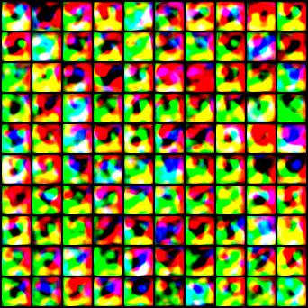
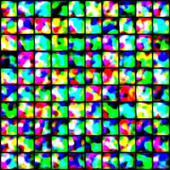
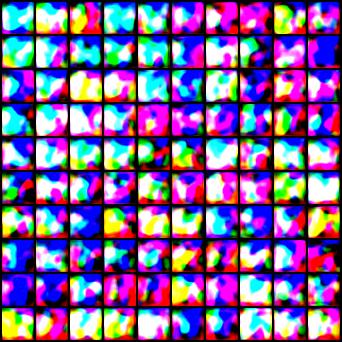
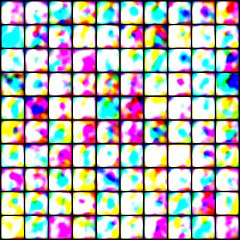
Figure 4: Generated Virtual Data for CIFAR-10, FMNIST and SVHN. Each figure has 90 data samples of the same class.

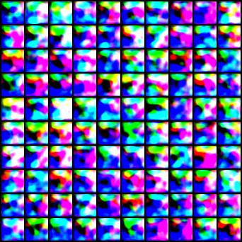
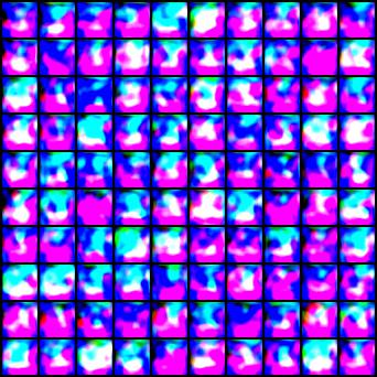
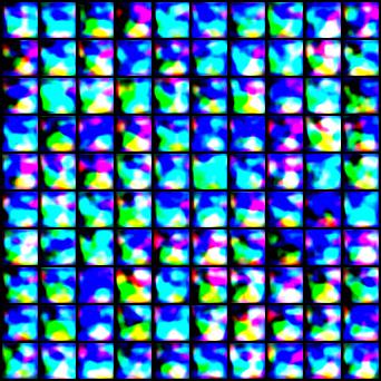
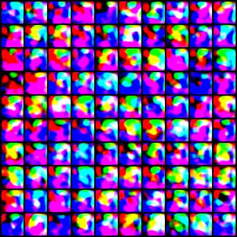
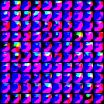
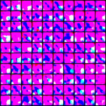
Figure 5: Generated Virtual Data for CIFAR-100. Due to space limitation, we only show 10 out of 100 classes.

Figure 7: Generated virtual dataset using ten simple decoders.

We show all convergence curves in Figure 14,  15,  16 and  17. One can see that nearly all experiments could benefit convergence acceleration from VHL.

Appendix D More Experiment Results and Discussion

D.1 Feature Shifts between Clients

We show more t-SNE visualization of feature distribution between client models in Figure 8,  9 and  10, and them of the server model in Figure 11,  12 and  13.

One can see that the clients can quickly learn to distinguish virtual data and attain the consensus on the feature expression of the virtual data of the same class (see Figure 9 (a) and Figure 10 (a)). Therefore, the subsequent local training based on the homogeneous virtual feature could benefit the consistent expression on the natural data.

One interesting observation is that only training with the virtual data also benefits FL. And clients also can more quickly learn consistent feature expression though such Naive VHL than through FedAvg (see Figure 9 (c) and Figure 10 (c)).

Another interesting finding is that, after local training, the features from one client are easily to be clustered together by t-SNE (see Figure 8 (a) and (b)), which means that these client models are greatly different. This happens even at the $999$-th communication round for FedAvg (see Figure 8 (d)).

(a) $9$-th round.

(b) $99$-th round.

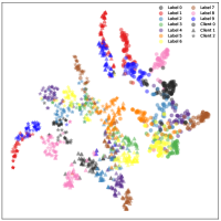
(c) $299$-th round.

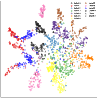
(d) $999$-th round.

Figure 8: Features of CIFAR10 test data of different client models without VHL.

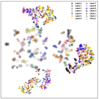
(a) $9$-th round.

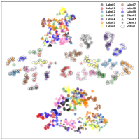
(b) $99$-th round.

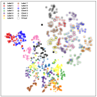
(c) $299$-th round.

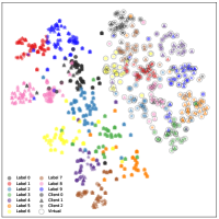
(d) at $999$-th round.

Figure 9: Features of CIFAR10 test data of different client models with Naive VHL.

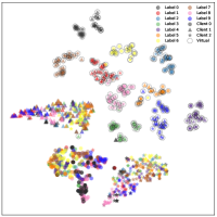
(a) $9$-th round.

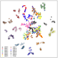
(b) $99$-th round.

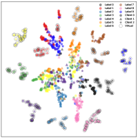
(c) $299$-th round.

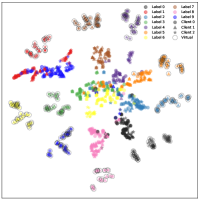
(d) at $999$-th round.

Figure 10: Features of CIFAR10 test data of different client models with VHL.

(a) $9$-th round.

(b) $99$-th round.

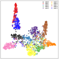
(c) $299$-th round.

(d) $999$-th round.

Figure 11: Features of CIFAR10 test data of server model without VHL.

(a) $9$-th round.

(b) $99$-th round.

(c) $299$-th round.

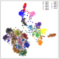
(d) at $999$-th round.

Figure 12: Features of CIFAR10 test data of server model with Naive VHL.

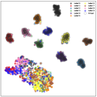
(a) $9$-th round.

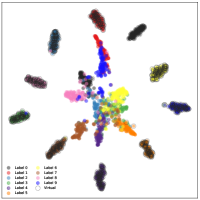
(b) $99$-th round.

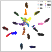
(c) $299$-th round.

(d) at $999$-th round.

Figure 13: Features of CIFAR10 test data of server model with VHL.

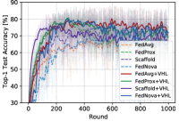
(a) $a=0.1$, $K=10$, $E=1$

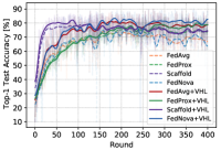
(b) $a=0.1$, $K=10$, $E=5$

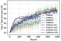
(c) $a=0.1$, $K=100$, $E=1$

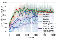
(d) $a=0.05$, $K=10$, $E=1$

Figure 14: Convergence comparison of CIFAR-10.

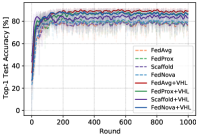
(a) $a=0.1$, $K=10$, $E=1$

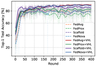
(b) $a=0.1$, $K=10$, $E=5$

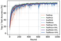
(c) $a=0.1$, $K=100$, $E=1$

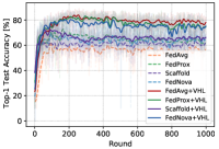
(d) $a=0.05$, $K=10$, $E=1$

Figure 15: Convergence comparison of FMNIST.

s

(a) $a=0.1$, $K=10$, $E=1$

(b) $a=0.1$, $K=10$, $E=5$

(c) $a=0.1$, $K=100$, $E=1$

(d) $a=0.05$, $K=10$, $E=1$

Figure 16: Convergence comparison of SVHN.

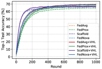
(a) $a=0.1$, $K=10$, $E=1$

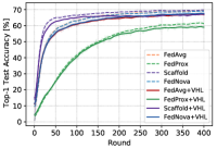
(b) $a=0.1$, $K=10$, $E=5$

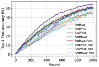
(c) $a=0.1$, $K=100$, $E=1$

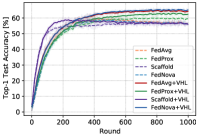
(d) $a=0.05$, $K=10$, $E=1$

Figure 17: Convergence comparison of CIFAR100.

D.2 More Facets of VHL

We provide more comparisons of convergence trends of three experiments, including loading pretrained models (Figure 18 (a)), VHL with different batch size (Figure 18 (b)), training accuracy with VHL but different virtual data (Figure 18 (c)).

Naive VHL. As summarized in Sec. 5.3, the naive VHL also could benefit FL. We discuss reasons of this in detail here. As pointed by (Luo et al., 2021; Yu et al., 2021), local training on local severe imbalanced dataset would lead to the severe preference of the classifer towards the local dominant classes. Due to this bias of classifer, the shallow layers of the model cannot learn good representations of the raw data. Therefore, introducing more common virtual data could alleviate such imbalance situation, even these virtual data has no relationship with the raw data. And the vision information owned by the virtual data could help clients learn better feature extractor, like (Baradad et al., 2021).

Batch Size of VHL. Similar with the contrastive learning (Khosla et al., 2020), because VHL needs to pull data of the same class together, the batch size impacts the effect of VHL. As shown in Table 6 and Figure 18 (b), larger batch size of virtual data improve both convergence and model performance. However, larger batch size means the extra calculation cost, which may be improved in the future.

Using Realistic Data. To our surprise, using the Tiny-ImageNet as the virtual data to conduct VHL cannot outperform using the virtual noise data. According to the classic transfer learning (Pan & Yang, 2009; Baradad et al., 2021), transferring knowledge from the realistic data should benefit generalization performance better than from the virtual images that seem like noise (see Figure 4,  5,  6 and  7). We suspect the reason is that the Tiny-ImageNet is more difficult to be separated than the generated virtual dataset, leading to the inconsistent features of the Tiny-ImageNet. Then the calibration loses its effect. To validate this conjecture, We plot the training accuracy of the virtual dataset in Figure 18 (c).

(a) Using Model Pretrained on Virtual Dataset.

(b) VHL with different $B_{v}$ of virtual dataset.

(c) Training ACC. on Virtual Dataset.

Figure 18: Convergence of more experiments.

D.3 Comparisons of Calculation Cost

As mentioned in section 5.5, training on the virtual data causes the extra calculation cost. Thus, similar with comparing the convergence speed, we compare the total calculation cost of different algorithms to achieve the target accuracy in Table 10. It shows how many data samples that each algorithm needs to process to achieve the target accuracy. We use $N_{total}$ and $R_{total}$ to represent the number of processed samples and the number of communication rounds to achieve the target accuracy, $R_{total}$ are shown in Table 1, 2, 4 and  5. And the $D_{data}$ represents the total size of all datasets from clients.

Note that for $E=1$ and $K=10$ setting, the $N_{total}=D_{data}\times R_{total}\times 0.5$, as the server randomly selects 5 clients each round. For $E=5$ and $K=10$ setting, $N_{total}=D_{data}\times R_{total}\times 0.5\times 5$, as each client conducts 5 local epochs before communication. For $E=1$ and $K=100$ setting, $N_{total}=D_{data}\times R_{total}\times 0.1$, as the server randomly selects 10 clients out of 100 clients each round. Because we sample virtual data with the same batch size as the natural data, the extra calculation cost is doubled for VHL.

Table 10 shows that for most of cases, VHL needs to process similar or less number of data samples to attain the target test accuracy. However, for CIFAR-100 dataset, VHL shows more calculation cost. This trend aligns with the communication, i.e. VHL shows less performance gains on CIFAR-100. To address this problem, one may consider reducing the sampling size of virtual data. Or, we may explore more interesting properties of VHL to make it computation-friendly, like the VFA discussed in section 5.3.

Table 10: Calculation cost ($\times D_{data}$ ) to achieve the target accuracy.

		Target ACC	w/(w/o) VHL	FedAvg	FedProx	SCAFFOLD	FedNova
CIFAR-10	$a=0.1$, $E=1$, $K=10$	100	without	143.5	94	145.5	175.5
			with	128	128	90	128
	$a=0.05$, $E=1$, $K=10$	100	without	205.5	100.5	Nan	Nan
			with	112	151	Nan	247
	$a=0.1$, $E=5$, $K=10$	100	without	637.5	Nan	165	317.5
			with	455	1275	225	335
	$a=0.1$, $E=1$, $K=100$	100	without	95.7	84.2	66.4	Nan
			with	77	65	95.8	110.8
FMNIST	$a=0.1$, $E=1$, $K=10$	100	without	59.5	67.5	71.5	41.5
			with	52	31	14	52
	$a=0.05$, $E=1$, $K=10$	100	without	212.5	20.5	Nan	269
			with	53	30	58	30
	$a=0.1$, $E=5$, $K=10$	100	without	695	Nan	262.5	482.5
			with	255	370	100	255
	$a=0.1$, $E=1$, $K=100$	100	without	65.8	49.1	Nan	Nan
			with	87.2	56.6	Nan	Nan
SVHN	$a=0.1$, $E=1$, $K=10$	100	without	125.5	Nan	Nan	125.5
			with	75	271	Nan	75
	$a=0.05$, $E=1$, $K=10$	100	without	178.5	Nan	Nan	370.5
			with	94	320	147	128
	$a=0.1$, $E=5$, $K=10$	100	without	327.5	Nan	Nan	405
			with	725	1755	1050	375
	$a=0.1$, $E=1$, $K=100$	100	without	61.8	61.8	64.3	Nan
			with	72.4	71.2	193.6	135.2
CIFAR-100	$a=0.1$, $E=1$, $K=10$	100	without	248.5	Nan	383	236
			with	384	617	294	384
	$a=0.05$, $E=1$, $K=10$	100	without	257	Nan	Nan	Nan
			with	354	482	Nan	320
	$a=0.1$, $E=5$, $K=10$	100	without	707.5	Nan	427.5	730
			with	1635	Nan	1455	Nan
	$a=0.1$, $E=1$, $K=100$	100	without	96.7	95.5	82.7	96.7
			with	143.4	143.4	131.2	159.4

References

- Acar et al. (2021) Acar, D. A. E., Zhao, Y., Matas, R., Mattina, M., Whatmough, P., and Saligrama, V. Federated learning based on dynamic regularization. In ICLR, 2021.
- Baradad et al. (2021) Baradad, M., Wulff, J., Wang, T., Isola, P., and Torralba, A. Learning to see by looking at noise. In NeurlPS, 2021.
- Ben-David et al. (2007) Ben-David, S., Blitzer, J., Crammer, K., Pereira, F., et al. Analysis of representations for domain adaptation. In NeurlPS, pp. 137–144, 2007.
- Ben-David et al. (2010) Ben-David, S., Blitzer, J., Crammer, K., Kulesza, A., Pereira, F., and Vaughan, J. W. A theory of learning from different domains. Machine learning, 79(1):151–175, 2010.
- Cai et al. (2021) Cai, K., Lei, X., Wei, J., and Xiao, X. Data synthesis via differentially private markov random fields. Proc. VLDB Endow., 14(11):2190–2202, 2021.
- Chang et al. (2019) Chang, H., Shejwalkar, V., Shokri, R., and Houmansadr, A. Cronus: Robust and heterogeneous collaborative learning with black-box knowledge transfer. arXiv preprint arXiv:1912.11279, 2019.
- Chatalic et al. (2021) Chatalic, A., Schellekens, V., Houssiau, F., de Montjoye, Y. A., Jacques, L., and Gribonval, R. Compressive learning with privacy guarantees. Information and Inference: A Journal of the IMA, 2021.
- Chen & Chao (2020) Chen, H.-Y. and Chao, W.-L. Fedbe: Making bayesian model ensemble applicable to federated learning. In NeurIPS, 2020.
- Croce et al. (2020) Croce, D., Castellucci, G., and Basili, R. Gan-bert: Generative adversarial learning for robust text classification with a bunch of labeled examples. In ACL, 2020.
- Diochnos et al. (2018) Diochnos, D., Mahloujifar, S., and Mahmoody, M. Adversarial risk and robustness: General definitions and implications for the uniform distribution. In NeurlPS, 2018.
- Franceschi et al. (2018) Franceschi, J.-Y., Fawzi, A., and Fawzi, O. Robustness of classifiers to uniform and gaussian noise. In AISTATS, 2018.
- Frénay & Verleysen (2013) Frénay, B. and Verleysen, M. Classification in the presence of label noise: a survey. IEEE transactions on neural networks and learning systems, 25(5):845–869, 2013.
- Ganin et al. (2016) Ganin, Y., Ustinova, E., Ajakan, H., Germain, P., Larochelle, H., Laviolette, F., Marchand, M., and Lempitsky, V. Domain-adversarial training of neural networks. The journal of machine learning research, 17(1):2096–2030, 2016.
- Goetz & Tewari (2020) Goetz, J. and Tewari, A. Federated learning via synthetic data. arXiv preprint arXiv:2008.04489, 2020.
- Gong et al. (2016) Gong, M., Zhang, K., Liu, T., Tao, D., Glymour, C., and Schölkopf, B. Domain adaptation with conditional transferable components. In ICML, 2016.
- Goodfellow et al. (2020) Goodfellow, I., Pouget-Abadie, J., Mirza, M., Xu, B., Warde-Farley, D., Ozair, S., Courville, A., and Bengio, Y. Generative adversarial networks. Communications of the ACM, 63(11):139–144, 2020.
- Hao et al. (2021) Hao, W., El-Khamy, M., Lee, J., Zhang, J., Liang, K. J., Chen, C., and Duke, L. C. Towards fair federated learning with zero-shot data augmentation. In CVPR, 2021.
- Hardt & Rothblum (2010) Hardt, M. and Rothblum, G. N. A multiplicative weights mechanism for privacy-preserving data analysis. In FOCS, 2010.
- Hardt et al. (2012) Hardt, M., Ligett, K., and Mcsherry, F. A simple and practical algorithm for differentially private data release. In NeurlPS, 2012.
- He et al. (2020) He, C., Li, S., So, J., Zhang, M., Wang, H., Wang, X., Vepakomma, P., Singh, A., Qiu, H., Shen, L., Zhao, P., Kang, Y., Liu, Y., Raskar, R., Yang, Q., Annavaram, M., and Avestimehr, S. Fedml: A research library and benchmark for federated machine learning. arXiv preprint arXiv:2007.13518, 2020.
- He et al. (2021) He, C., Shah, A. D., Tang, Z., Sivashunmugam, D. F. N., Bhogaraju, K., Shimpi, M., Shen, L., Chu, X., Soltanolkotabi, M., and Avestimehr, S. Fedcv: A federated learning framework for diverse computer vision tasks. arXiv preprint arXiv:2111.11066, 2021.
- He et al. (2016) He, K., Zhang, X., Ren, S., and Sun, J. Deep residual learning for image recognition. In CVPR, 2016.
- Hsu et al. (2019) Hsu, T. H., Qi, H., and Brown, M. Measuring the effects of non-identical data distribution for federated visual classification. arXiv preprint arxiv: 1909.06335, 2019.
- Hsu et al. (2020) Hsu, T.-M. H., Qi, H., and Brown, M. Federated visual classification with real-world data distribution. In ECCV, 2020.
- Huang et al. (2019) Huang, X., Wang, P., Cheng, X., Zhou, D., Geng, Q., and Yang, R. The apolloscape open dataset for autonomous driving and its application. IEEE transactions on pattern analysis and machine intelligence, 42(10):2702–2719, 2019.
- Jeong et al. (2018) Jeong, E., Oh, S., Kim, H., Park, J., Bennis, M., and Kim, S.-L. Communication-efficient on-device machine learning: Federated distillation and augmentation under non-iid private data. 2018.
- Jin et al. (2020) Jin, X., Lan, C., Zeng, W., Chen, Z., and Zhang, L. Style normalization and restitution for generalizable person re-identification. In CVPR, 2020.
- Johnson et al. (2018) Johnson, N., Near, J. P., and Song, D. Towards practical differential privacy for sql queries. Proceedings of the VLDB Endowment, 11(5):526–539, 2018.
- Kairouz et al. (2021) Kairouz, P., McMahan, H. B., Avent, B., Bellet, A., Bennis, M., Bhagoji, A. N., Bonawitz, K., Charles, Z., Cormode, G., Cummings, R., et al. Advances and open problems in federated learning. Found. Trends Mach. Learn., 14(1-2):1–210, 2021.
- Karimireddy et al. (2020) Karimireddy, S. P., Kale, S., Mohri, M., Reddi, S., Stich, S., and Suresh, A. T. SCAFFOLD: Stochastic controlled averaging for federated learning. In ICML, 2020.
- Karras et al. (2019) Karras, T., Laine, S., and Aila, T. A style-based generator architecture for generative adversarial networks. In CVPR, 2019.
- Karras et al. (2020) Karras, T., Laine, S., Aittala, M., Hellsten, J., Lehtinen, J., and Aila, T. Analyzing and improving the image quality of StyleGAN. In CVPR, 2020.
- Khosla et al. (2020) Khosla, P., Teterwak, P., Wang, C., Sarna, A., Tian, Y., Isola, P., Maschinot, A., Liu, C., and Krishnan, D. Supervised contrastive learning. 2020.
- Koltchinskii & Panchenko (2002) Koltchinskii, V. and Panchenko, D. Empirical margin distributions and bounding the generalization error of combined classifiers. The Annals of Statistics, 30(1):1–50, 2002.
- Krizhevsky & Hinton (2009) Krizhevsky, A. and Hinton, G. Learning multiple layers of features from tiny images. Master’s thesis, 2009.
- Le & Yang (2015) Le, Y. and Yang, X. Tiny imagenet visual recognition challenge. CS 231N, 7(7):3, 2015.
- Lei et al. (2021) Lei, Q., Hu, W., and Lee, J. Near-optimal linear regression under distribution shift. In ICML, 2021.
- Li & Wang (2019) Li, D. and Wang, J. Fedmd: Heterogenous federated learning via model distillation. arXiv preprint arXiv:1910.03581, 2019.
- Li et al. (2021a) Li, Q., Diao, Y., Chen, Q., and He, B. Federated learning on non-iid data silos: An experimental study. arXiv preprint arXiv:2102.02079, 2021a.
- Li et al. (2021b) Li, Q., He, B., and Song, D. Model-contrastive federated learning. In CVPR, 2021b.
- Li et al. (2020a) Li, T., Sahu, A. K., Zaheer, M., Sanjabi, M., Talwalkar, A., and Smith, V. Federated optimization in heterogeneous networks. In MLSys, 2020a.
- Li et al. (2020b) Li, X., Huang, K., Yang, W., Wang, S., and Zhang, Z. On the convergence of fedavg on non-iid data. In ICLR, 2020b.
- Lin et al. (2020) Lin, T., Kong, L., Stich, S. U., and Jaggi, M. Ensemble distillation for robust model fusion in federated learning. In NeurIPS, 2020.
- Liu et al. (2020) Liu, F., Zhang, G., and Lu, J. Heterogeneous domain adaptation: An unsupervised approach. IEEE transactions on neural networks and learning systems, 31(12):5588–5602, 2020.
- Long et al. (2013) Long, M., Wang, J., Ding, G., Sun, J., and Yu, P. S. Transfer feature learning with joint distribution adaptation. In ICCV, 2013.
- Long et al. (2017) Long, M., Zhu, H., Wang, J., and Jordan, M. I. Deep transfer learning with joint adaptation networks. In ICML, 2017.
- Long et al. (2021) Long, Y., Wang, B., Yang, Z., Kailkhura, B., Zhang, A., Gunter, C., and Li, B. G-pate: Scalable differentially private data generator via private aggregation of teacher discriminators. 2021.
- Luo et al. (2019) Luo, J., Wu, X., Luo, Y., Huang, A., Huang, Y., Liu, Y., and Yang, Q. Real-world image datasets for federated learning. arXiv preprint arXiv:1910.11089, 2019.
- Luo et al. (2021) Luo, M., Chen, F., Hu, D., Zhang, Y., Liang, J., and Feng, J. No fear of heterogeneity: Classifier calibration for federated learning with non-IID data. In NeurlPS, 2021.
- McMahan et al. (2017) McMahan, B., Moore, E., Ramage, D., Hampson, S., and y Arcas, B. A. Communication-efficient learning of deep networks from decentralized data. In AISTATS, 2017.
- Miyato et al. (2018) Miyato, T., Maeda, S.-i., Koyama, M., and Ishii, S. Virtual adversarial training: a regularization method for supervised and semi-supervised learning. IEEE transactions on pattern analysis and machine intelligence, 41(8):1979–1993, 2018.
- Netzer et al. (2011) Netzer, Y., Wang, T., Coates, A., Bissacco, A., Wu, B., and Ng, A. Y. Reading digits in natural images with unsupervised feature learning. In NIPS Workshop on Deep Learning and Unsupervised Feature Learning 2011, 2011.
- Pan & Yang (2009) Pan, S. J. and Yang, Q. A survey on transfer learning. IEEE Transactions on knowledge and data engineering, 22(10):1345–1359, 2009.
- Pan et al. (2010) Pan, S. J., Tsang, I. W., Kwok, J. T., and Yang, Q. Domain adaptation via transfer component analysis. IEEE transactions on neural networks, 22(2):199–210, 2010.
- Polyzotis et al. (2017) Polyzotis, N., Roy, S., Whang, S. E., and Zinkevich, M. Data management challenges in production machine learning. In SIGMOD, 2017.
- Qiu et al. (2017) Qiu, W., Zhong, F., Zhang, Y., Qiao, S., Xiao, Z., Kim, T. S., and Wang, Y. Unrealcv: Virtual worlds for computer vision. In ACM Multimedia, 2017.
- Quiñonero-Candela et al. (2008) Quiñonero-Candela, J., Sugiyama, M., Schwaighofer, A., and Lawrence, N. D. Dataset shift in machine learning. Mit Press, 2008.
- Reddi et al. (2021) Reddi, S. J., Charles, Z., Zaheer, M., Garrett, Z., Rush, K., Konečný, J., Kumar, S., and McMahan, H. B. Adaptive federated optimization. In ICLR, 2021.
- Sehwag et al. (2021) Sehwag, V., Mahloujifar, S., Handina, T., Dai, S., Xiang, C., Chiang, M., and Mittal, P. Improving adversarial robustness using proxy distributions. arXiv preprint arXiv:2104.09425, 2021.
- Shin et al. (2020) Shin, M., Hwang, C., Kim, J., Park, J., Bennis, M., and Kim, S.-L. Xor mixup: Privacy-preserving data augmentation for one-shot federated learning. arXiv preprint arXiv:2006.05148, 2020.
- Tang et al. (2021) Tang, Z., Hu, Z., Shi, S., Cheung, Y.-M., Jin, Y., Ren, Z., and Chu, X. Data resampling for federated learning with non-iid labels. In FTL-IJCAI’21, 2021.
- Tramer & Boneh (2021) Tramer, F. and Boneh, D. Differentially private learning needs better features (or much more data). In ICLR, 2021.
- van der Maaten & Hinton (2008) van der Maaten, L. and Hinton, G. Visualizing data using t-sne. Journal of Machine Learning Research, 9(86):2579–2605, 2008.
- Wang et al. (2020) Wang, J., Liu, Q., Liang, H., Joshi, G., and Poor, H. V. Tackling the objective inconsistency problem in heterogeneous federated optimization. In NeurlPS, 2020.
- Wang et al. (2021) Wang, J., Charles, Z., Xu, Z., Joshi, G., McMahan, H. B., Al-Shedivat, M., Andrew, G., Avestimehr, S., Daly, K., Data, D., et al. A field guide to federated optimization. arXiv preprint arXiv:2107.06917, 2021.
- Xiao et al. (2017) Xiao, H., Rasul, K., and Vollgraf, R. Fashion-mnist: a novel image dataset for benchmarking machine learning algorithms. arXiv preprint arXiv:1708.07747, 2017.
- Yang et al. (2021) Yang, K., Zhou, T., Zhang, Y., Tian, X., and Tao, D. Class-disentanglement and applications in adversarial detection and defense. In NeurIPS, 2021.
- Yang et al. (2018) Yang, T., Andrew, G., Eichner, H., Sun, H., Li, W., Kong, N., Ramage, D., and Beaufays, F. Applied federated learning: Improving google keyboard query suggestions. arXiv preprint arXiv:1812.02903, 2018.
- Yoon et al. (2021) Yoon, T., Shin, S., Hwang, S. J., and Yang, E. Fedmix: Approximation of mixup under mean augmented federated learning. In ICLR, 2021.
- Yu et al. (2021) Yu, F., Zhang, W., Qin, Z., Xu, Z., Wang, D., Liu, C., Tian, Z., and Chen, X. Fed2: Feature-aligned federated learning. In SIGKDD, 2021.
- Yurochkin et al. (2019) Yurochkin, M., Agarwal, M., Ghosh, S., Greenewald, K., Hoang, N., and Khazaeni, Y. Bayesian nonparametric federated learning of neural networks. In ICML, 2019.
- Zhang et al. (2013) Zhang, K., Schölkopf, B., Muandet, K., and Wang, Z. Domain adaptation under target and conditional shift. In ICML, 2013.
- Zhao et al. (2019) Zhao, H., Des Combes, R. T., Zhang, K., and Gordon, G. On learning invariant representations for domain adaptation. In ICML, 2019.
- Zhao et al. (2021) Zhao, N., Wu, Z., Lau, R. W. H., and Lin, S. What makes instance discrimination good for transfer learning? In ICLR, 2021.
- Zhao et al. (2018) Zhao, Y., Li, M., Lai, L., Suda, N., Civin, D., and Chandra, V. Federated learning with non-iid data. arXiv preprint arXiv:1806.00582, 2018.