Efficient and Scalable Parametric High-Order Portfolios Design via the Skew-$t$ Distribution

Abstract

Since Markowitz’s mean-variance framework, optimizing a portfolio that strikes a trade-off between maximizing profit and minimizing risk has been ubiquitous in the financial industry. Initially, profit and risk were measured by the first two moments of the portfolio’s return, a.k.a. the mean and variance, which are sufficient to characterize a Gaussian distribution. However, it is broadly believed that the first two moments are not enough to capture the characteristics of the returns’ behavior, which have been recognized to be asymmetric and heavy-tailed. Although portfolio designs involving the third and fourth moments, i.e., skewness and kurtosis, have been demonstrated to outperform the conventional mean-variance framework, they present non-trivial challenges. Specifically, in the classical framework, the memory and computational cost of computing the skewness and kurtosis grow sharply with the number of assets. To alleviate the difficulty in high-dimensional problems, we consider an alternative expression for high-order moments based on parametric representations via a generalized hyperbolic skew-$t$ distribution. Then, we reformulate the high-order portfolio optimization problem as a fixed-point problem and propose a robust fixed-point acceleration algorithm that solves the problem in an efficient and scalable manner. Empirical experiments also attest to the efficiency of our proposed high-order portfolio optimization framework, which presents low complexity and significantly outperforms the state-of-the-art methods by $2\sim 4$ orders of magnitude.

I Introduction

Modern portfolio theory (MPT), pioneered by Harry Markowitz [1], strives to reaching a trade-off between minimizing the risk of the portfolio and maximizing its profit. For the convenience of modeling the profit and risk, the assets’ returns are conventionally assumed to follow a Gaussian distribution. The Gaussian distribution was embraced in early research for a number of reasons [2]. First of all, it is straightforward to describe the data using the Gaussian distribution. The mean vector $\boldsymbol{\mu}$ and covariance matrix $\boldsymbol{\Sigma}$, which are the parameters of the Gaussian distribution, can be obtained via numerous estimation methods. Moreover, the mathematical expression of profit and risk are henceforth simple enough such that the resultant portfolio designs are convenient from the perspective of optimization. However, the mean and variance, a.k.a. the first- and second-order moments, are usually not sufficient to capture the characteristics of the assets’ returns [3, 4]. It is widely acknowledged that empirical observations of stock data exhibit asymmetry and fat tails that can be barely described by a Gaussian distribution [5, 6, 7, 8]. In light of these deficiencies, a number of empirical evidence advocates the incorporation of the high-order moments into portfolio design [9, 10].

The concerns of skewness and kurtosis, a.k.a. third- and fourth-order moments, have been raised for decades [11]. Typically, higher skewness is preferred as it reduces extreme values on the side of losses and increases them on the side of gains. Whereas the kurtosis measures dispersion which is something undesirable that increases the uncertainty of returns [12, 13, 14]. A detailed discussion can be found in [13]. Therefore, portfolio designs should also aspire to achieve high skewness and low kurtosis. This trade-off was then naturally formulated as a mean-variance-skewness-kurtosis (MVSK) framework [15].

Although there are many compelling advantages of involving skewness and kurtosis [16, 17], solving high-order portfolio optimization problems is non-trivial. Given a problem formulation to specify the trade-off, a typical high-order portfolio design consists of a model to characterize the high-order moments and optimization algorithms to solve the problem. Each of these modules can be a limiting factor in the overall practicability of the framework. In this paper, we start from the classical MVSK problem formulation. Then, the first fundamental problem is how to model the skewness and kurtosis of the portfolio return. The conventional approach models the skewness and kurtosis via the vanilla co-skewness matrix $\boldsymbol{\Phi}\in\mathbb{R}^{N\times N^{2}}$ and co-kurtosis matrix $\boldsymbol{\Psi}\in\mathbb{R}^{N\times N^{3}}$. However, this non-parametric modeling suffers a lot from the dimensionality problem [18], which might not be critical on variance but is severely exacerbated on estimating skewness and kurtosis. For example, to obtain $\boldsymbol{\Phi}$ and $\boldsymbol{\Psi}$ when $N=100$, we need to estimate more than $170$ thousand and $4$ million parameters, respectively. As the number of parameters is significantly larger than the number of samples, the estimation error is inevitably large [19]. In addition, the storage burden is also exceptionally heavy. Any mathematical manipulations involving $\boldsymbol{\Phi}$ and $\boldsymbol{\Psi}$ would demand prohibitive computational resources and are thus not applicable to high-dimensional problems.

Apart from the high computational cost due to the matrices $\boldsymbol{\Phi}$ and $\boldsymbol{\Psi}$, the third moment of the portfolio return is non-convex, making it difficult to optimize. The existing methods in the literature can be roughly classified into three major categories: zeroth-order, first-order, and second-order methods. The zeroth-order methods [20] usually iteratively improve the objective values via repetitive function evaluations. For instance, the differential evolution [21] and genetic algorithms [22] iteratively improve solutions via searching in the feasible region. Usually, zeroth-order searching algorithms are often criticized for their mediocre performance on the computational cost. The first-order methods make use of the first-order derivative of the objective function. Some classical examples include the difference-of-convex (DC) algorithms [23, 24] and some Majorization-Minimization algorithms [25]. However, the first-order methods may need quite a large number of iterations to converge. In contrast, the second-order methods improve the description of the descent direction by incorporating the second-order derivative of the objective function. For example, the Q-MVSK algorithm [25] presents a significantly faster convergence rate than the first-order methods. However, the per-iteration cost of second-order methods is prohibitive as computing the Hessian has dramatically high complexity.

In summary, due to the computationally expensive modeling of high-order moments and the absence of practical optimization algorithms, the current MVSK framework can only produce high-order portfolios in low-dimensional problems. To address these limitations, in this paper, we present a novel high-order portfolio design framework that is both efficient and scalable. Our contributions are mainly twofold:

1. We adopt a parametric model to significantly reduce the memory and computational cost of obtaining the high-order moments of the portfolio return. The proposed method accommodates the high-dimensional scenarios by fitting the data via a generalized hyperbolic skew-$t$ distribution.

2. We propose a practical algorithm based on a robust fixed point acceleration strategy to solve the high-order portfolios. The numerical experiments demonstrate that the proposed algorithms are significantly more efficient and scalable than the state-of-the-art solvers.

The structure of this paper is as follows. In Section II, we first introduce the high-order portfolio optimization problems and illustrate the current difficulties. In Section III, we present an efficient approach to compute the skewness and kurtosis using a generalized hyperbolic skew-$t$ distribution. The parametric distribution allows a faster way of computing high-order moments of the portfolio. In Section IV, we propose efficient algorithms to solve the MVSK portfolios based on fixed point acceleration strategy. Additionally, in Section V, we show that the proposed algorithm can be easily generalized into the MVSK-Tilting portfolio. Then, we elaborate the performance of proposed high-order portfolio design framework in Section VI. Finally, we summarize the conclusions in section VII.

II Problem formulations

II-A MVSK Portfolios

Let $\mathbf{r}\in\mathbb{R}^{N}$ denote the log-returns of $N$ assets and $\mathbf{w}\in\mathbb{R}^{N}$ denote the portfolio weights. The classical mean-variance portfolio optimization problem is formulated as

$$\begin{array}[]{ll}\underset{\mathbf{w}}{\mathsf{minimize}}&-\phi_{1}\left(\mathbf{w}\right)+\lambda\phi_{2}\left(\mathbf{w}\right)\\ \mathsf{subject}\text{ }\mathsf{to}&\mathbf{w}\in\mathcal{W},\end{array}$$ (1)

where $\phi_{1}\left(\mathbf{w}\right)$ refers to the first central moment, a.k.a. the mean of the portfolio return, i.e.,

$$\phi_{1}\left(\mathbf{w}\right)=\mathbb{E}\left[\mathbf{w}^{T}\mathbf{r}\right],$$ (2)

$\phi_{2}\left(\mathbf{w}\right)$ is the second central moment, which is the variance of the portfolio return, i.e.,

$$\phi_{2}\left(\mathbf{w}\right)=\mathbf{\mathbb{E}}\left[\left(\mathbf{w}^{T}\mathbf{r}-\mathbb{E}\left[\mathbf{w}^{T}\mathbf{r}\right]\right)^{2}\right],$$ (3)

$\lambda>0$ is a risk-aversion coefficient, and $\mathcal{W}$ represents the feasible set of the portfolio weights. In the paper, we consider no-shorting. Therefore, $\mathcal{W}$ is a unit simplex denoted as

$$\mathcal{W}=\left\{\mathbf{w}\left|\mathbf{1}^{T}\mathbf{w}=1,\mathbf{w}\geq\mathbf{0}\right.\right\}.$$ (4)

Now, we incorporate the third and fourth central moments of the portfolio return, i.e.,

$$\phi_{3}\left(\mathbf{w}\right) =\mathbf{\mathbb{E}}\left[\left(\mathbf{w}^{T}\mathbf{r}-\mathbb{E}\left[\mathbf{w}^{T}\mathbf{r}\right]\right)^{3}\right],$$ (5)

$$\phi_{4}\left(\mathbf{w}\right) =\mathbf{\mathbb{E}}\left[\left(\mathbf{w}^{T}\mathbf{r}-\mathbb{E}\left[\mathbf{w}^{T}\mathbf{r}\right]\right)^{4}\right],$$

into the portfolio selection. This directly extends the mean-variance portfolio into a mean-variance-skewness-kurtosis (MVSK) portfolio, formulated as follows

$$\begin{array}[]{ll}\underset{\mathbf{w}}{\mathsf{minimize}}&f\left(\mathbf{w}\right)=-\lambda_{1}\phi_{1}\left(\mathbf{w}\right)+\lambda_{2}\phi_{2}\left(\mathbf{w}\right)\\ &\quad\quad\quad\,\,\,\,-\lambda_{3}\phi_{3}\left(\mathbf{w}\right)+\lambda_{4}\phi_{4}\left(\mathbf{w}\right)\\ \mathsf{subject}\text{ }\mathsf{to}&\mathbf{w}\in\mathcal{W},\end{array}$$ (6)

where $\lambda_{1},\lambda_{2},\lambda_{3},\lambda_{4}$ are the non-negative parameters controlling the relative importance of individual moments.

II-B Current Difficulties

Among many difficulties regarding high-order portfolio designs, the most fundamental bottleneck is the prohibitive cost of computing high-order central moments using the non-parametric representation. Namely, the conventional way applies the following formulas to characterize the co-skewness and co-kurtosis matrices,

$$\boldsymbol{\Phi} =\mathbb{E}\left[\left(\mathbf{r}-\boldsymbol{\mu}\right)\left(\mathbf{r}-\boldsymbol{\mu}\right)\otimes\left(\mathbf{r}-\boldsymbol{\mu}\right)\right],$$

$$\boldsymbol{\Psi} =\mathbb{E}\left[\left(\mathbf{r}-\boldsymbol{\mu}\right)\left(\mathbf{r}-\boldsymbol{\mu}\right)\otimes\left(\mathbf{r}-\boldsymbol{\mu}\right)\otimes\left(\mathbf{r}-\boldsymbol{\mu}\right)\right],$$ (7)

where $\boldsymbol{\mu}=\mathbb{E}\left[\mathbf{r}\right]$. As shown in Table I, the costs for storing $\boldsymbol{\Phi}$ and $\boldsymbol{\Psi}$ have a high complexity. This means that we may not be able to set up these matrices when the problem dimension is large.

Table I: Conventional non-parametric representations of high-order moments.

	Number of parameters	Memory
	to estimate	complexity
Co-skewness $\boldsymbol{\Phi}$	$\frac{1}{6}N\left(N+1\right)\left(N+2\right)$	$\mathcal{O}\left(N^{3}\right)$
Co-kurtosis $\boldsymbol{\Psi}$	$\frac{1}{24}N\left(N+1\right)\left(N+2\right)\left(N+3\right)$	$\mathcal{O}\left(N^{4}\right)$

In addition, the non-parametric approach also poses tremendous challenges in computing the objectives values, gradients, and the Hessian of the third and fourth central moments for a given portfolio [25]. Here, we exhibit the corresponding complexities in Table II. As a result, existing first-order methods could not be efficient as they often require many iterations to converge while per-iteration cost is very high. On the other hand, existing second-order methods are not scalable because the complexity of computing $\nabla^{2}\phi_{4}\left(\mathbf{w}\right)$ is $\mathcal{O}\left(N^{5}\right)$.

Table II: Formulations and computational complexity of computing high-order moments in non-parametric way.

		Formulation	Complexity
3rd	$\phi_{3}\left(\mathbf{w}\right)$	$\mathbf{w}^{T}\boldsymbol{\Phi}\left(\mathbf{w}\otimes\mathbf{w}\right)$	$\mathcal{O}\left(N^{3}\right)$
central	$\nabla\phi_{3}\left(\mathbf{w}\right)$	$3\boldsymbol{\Phi}\left(\mathbf{w}\otimes\mathbf{w}\right)$	$\mathcal{O}\left(N^{3}\right)$
moment	$\nabla^{2}\phi_{3}\left(\mathbf{w}\right)$	$6\boldsymbol{\Phi}\left(\mathbf{I}\otimes\mathbf{w}\right)$	$\mathcal{O}\left(N^{4}\right)$
4th	$\phi_{4}\left(\mathbf{w}\right)$	$\mathbf{w}^{T}\boldsymbol{\Psi}\left(\mathbf{w}\otimes\mathbf{w}\otimes\mathbf{w}\right)$	$\mathcal{O}\left(N^{4}\right)$
central	$\nabla\phi_{4}\left(\mathbf{w}\right)$	$4\boldsymbol{\Psi}\left(\mathbf{w}\otimes\mathbf{w}\otimes\mathbf{w}\right)$	$\mathcal{O}\left(N^{4}\right)$
moment	$\nabla^{2}\phi_{4}\left(\mathbf{w}\right)$	$12\boldsymbol{\Psi}\left(\mathbf{I}\otimes\mathbf{w}\otimes\mathbf{w}\right)$	$\mathcal{O}\left(N^{5}\right)$

Therefore, in the next section, we would present a parametric approach to model the skewness and kurtosis such that the concerns discussed above can be significantly eliminated.

III Modeling high-order moments using generalized hyperbolic multivariate skew-$t$ distribution

In this section, we illustrate how to apply a parametric distribution to model the data and derive the high-order moments from the parametric model. To be more specific, this approach assumes that the assets’ returns follow a multivariate generalized hyperbolic skew-$t$ distribution. Then, high-order moments can be represented using the parameters of the fitted distribution. To proceed, we will first present some preliminary knowledge of the generalized hyperbolic skew-$t$ distribution, followed by the derivation of efficient methods for computing high-order moments based on this distribution.

III-A ghMST Distribution

The generalized hyperbolic multivariate skew-$t$ (ghMST) distribution [26, 27], is a sub-class of the generalized hyperbolic distribution [28], which is often used in economics to model the data with skewness and heavy tails [29, 30, 31, 32].

Suppose that a $N$-dimensional random vector $\mathbf{x}$ follows the ghMST distribution, i.e., $\mathbf{x}\sim\textsf{ghMST}\left(\boldsymbol{\mu},\boldsymbol{\Sigma},\boldsymbol{\gamma},\nu\right)$. It has the probability density function (pdf)

$$\begin{array}[]{rl}f_{\textsf{ghMST}}\left(\mathbf{x}\left|\boldsymbol{\mu},\boldsymbol{\Sigma},\boldsymbol{\gamma},\nu\right.\right)=\frac{e^{\left(\mathbf{x}-\boldsymbol{\mu}\right)^{T}\boldsymbol{\Sigma}^{-1}\boldsymbol{\gamma}}}{\left(2\pi\right)^{\frac{N}{2}}\left|\boldsymbol{\Sigma}\right|{}^{\frac{1}{2}}}\cdot 2\left(\frac{\nu}{2}\right)^{\frac{\nu}{2}}\cdot\frac{1}{\Gamma\left(\frac{\nu}{2}\right)}\cdot\\ \text{ }\left(\frac{\chi+Q\left(\mathbf{x}\right)}{\boldsymbol{\gamma}^{T}\boldsymbol{\Sigma}^{-1}\boldsymbol{\gamma}}\right)^{-\frac{\nu+N}{4}}\cdot K_{-\frac{\nu+N}{2}}\left(\sqrt{\left(\nu+Q\left(\mathbf{x}\right)\right)\left(\boldsymbol{\gamma}^{T}\boldsymbol{\Sigma}^{-1}\boldsymbol{\gamma}\right)}\right),\end{array}$$ (8)

where $\nu\in\mathbb{R}_{++}$ is the degree of freedom, $\boldsymbol{\mu}\in\mathbb{R}^{N}$ is the location vector, $\boldsymbol{\gamma}\in\mathbb{R}^{N}$ is the skewness vector, $\boldsymbol{\Sigma}\in\mathbb{R}^{N\times N}$ is the scatter matrix, $\Gamma$ is the gamma function, $Q\left(\mathbf{x}\right)=\left(\mathbf{x}-\boldsymbol{\mu}\right)^{T}\boldsymbol{\Sigma}^{-1}\left(\mathbf{x}-\boldsymbol{\mu}\right)$, and $K_{\lambda}$ is the modified Bessel function of the second kind with index $\lambda$ [33].

Remark 1.

In the following contexts, $\boldsymbol{\mu}$ and $\boldsymbol{\Sigma}$ refer to the parameters of ghMST distribution, that is, to the location vector and scatter matrix and not to the mean vector and covariance matrix.

Interestingly, the ghMST distribution can be represented in a hierarchical structure as

$$\mathbf{x}|\tau \overset{\text{i.i.d}}{\sim}\,\,\mathcal{N}\left(\boldsymbol{\mu}+\frac{1}{\tau}\boldsymbol{\gamma},\frac{1}{\tau}\boldsymbol{\Sigma}\right),$$ (9)

$$\tau \overset{\text{i.i.d}}{\sim}\,\,\text{Gamma}\left(\frac{\nu}{2},\frac{\nu}{2}\right),$$

where $\mathcal{N}\left(\tilde{\boldsymbol{\mu}},\tilde{\boldsymbol{\Sigma}}\right)$ denotes the multivariate Gaussian distribution with mean vector $\tilde{\boldsymbol{\mu}}$ and covariance matrix $\tilde{\boldsymbol{\Sigma}}$, and $\text{Gamma}\left(a,b\right)$ represents the gamma distribution of shape $a$ and rate $b$.

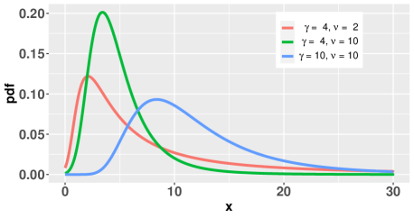
Figure 1: Illustrations for the univariate generalized hyperbolic skew-$t$ distribution $(\mu=0$, $\Sigma=1)$.

Figure 1 illustrates the skewness and fat-tailness under the ghMST distribution. When $\boldsymbol{\gamma}$ is fixed, the higher the value of $\nu$, the thinner the tails. When $\nu$ is fixed, the larger the value of $\boldsymbol{\gamma}$, the heavier the skewness. Henceforth, the third- and fourth-moments are naturally embedded into the parameters of the distribution.

In the literature, some restricted multivariate skew-$t$ (rMST) distributions [39] are also capable of modeling asymmetry and fat-tailness. In this paper, we choose to use the ghMST distribution for two reasons. Foremost, the ghMST distribution is the only skew-$t$ distribution that we can fit within a reasonable amount of time under high-dimensional settings [38, 40]. The details of fitting time are discussed in Appendix -A. In short, existing implementations may take a number of minutes to fit the rMST distribution when $N\geq 30$. In contrast, existing EM algorithms can efficiently fit the ghMST distribution with thousands of assets in few seconds [26, 44, 45]. When $N=20$, fitting a ghMST distribution is over four orders of magnitude faster than fitting an rMST distribution.

On the other hand, rMST distributions do not provide better out-of-sample fitting performance. To show this, we conduct a simple experiment as follows. In each realization, we randomly select $N$ assets from SP$500$ stock list. Then, we randomly pick the data from $15N$ continuous trading days to form the data set $\mathcal{D}$. Without shuffle, $\mathcal{D}$ is split into training set $\mathcal{D}_{\text{train}}$ and test set $\mathcal{D}_{\text{test}}$ by assigning the $2/3$ data to the former and the remaining $1/3$ to the latter. For each distribution, the optimal parameters are obtained via the training set

$$\begin{array}[]{cc}&\boldsymbol{\Theta}^{\star}=\arg\max_{\boldsymbol{\Theta}}\text{ }\mathcal{L}\left(\mathcal{D}_{\text{train}};\boldsymbol{\Theta}\right).\end{array}$$ (10)

Then we compute the out-of-sample normalized log-likelihood on the test set as $\frac{1}{5N^{2}}\mathcal{L}_{\text{test}}\left(\mathcal{D}_{\text{test}};\boldsymbol{\Theta}^{\star}\right).$ We repeat the experiments $50$ times for each problem dimension. Figure 2 shows that the ghMST distribution gives a higher average likelihood values when $N$ goes large. As it is difficult to differentiate their obtained likelihoods, the ghMST distribution appears to be the best choice for characterizing high-order moments due to its significantly more efficient estimation.

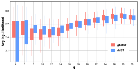
Figure 2: Out-of-sample log-likelihood for the restricted skew-t (rMST) and generalized hyperbolic skew-$t$ (ghMST) distributions.

III-B Computing high-order moments under ghMST distribution

Incorporating the ghMST distribution into the design of high-order portfolios also makes it convenient to manipulate the high-order moments, i.e., skewness and kurtosis. In this subsection, we highlight two advantages of using the parametric ghMST distribution. Firstly, it allows for low-memory representation of the co-moments of the asset return. Secondly, it provides more efficient computation of the skewness and kurtosis to the portfolio returns.

In the conventional framework, before we compute the high-order moments of portfolio returns, we need to store large matrices, including $\boldsymbol{\Phi}$ and $\boldsymbol{\Psi}$. Now, we suppose that a random vector $\mathbf{r}$ follows a ghMST distribution. Then, according to Lemma 2, the high-order moments can be easily computed from the parameter set $\boldsymbol{\Theta}=\left\{\boldsymbol{\mu},\boldsymbol{\Sigma},\boldsymbol{\gamma},\nu\right\}$, which is significantly smaller than $\boldsymbol{\Phi}$ and $\boldsymbol{\Psi}$. As a result, the memory complexity is reduced from $\mathcal{O}\left(N^{4}\right)$ to $\mathcal{O}\left(N^{2}\right)$.

Lemma 2.

Assuming a random vector $\mathbf{r}\sim\textsf{ghMST}\left(\boldsymbol{\mu},\boldsymbol{\Sigma},\boldsymbol{\gamma},\nu\right)$, then the mean and covariance of $\mathbf{r}$ are given as

$$\mathbb{E}\left[\mathbf{r}\right] =\boldsymbol{\mu}+a_{1}\boldsymbol{\gamma},$$ (11)

$$\text{Cov}\left[\mathbf{r}\right] =a_{21}\boldsymbol{\Sigma}+a_{22}\boldsymbol{\gamma\gamma}^{T},$$

where $a_{1}=\frac{\nu}{\nu-2}$, $a_{21}=\frac{\nu}{\nu-2}$, and $a_{22}=\frac{2\nu^{2}}{\left(\nu-2\right)^{2}\left(\nu-4\right)}$ are scalar coefficients decided by $\nu$. The third moment co-skewness matrix $\boldsymbol{\Phi}$ is expressed as

$$\Phi_{i,\left(j-1\right)\times N+k} =a_{31}\gamma_{i}\gamma_{j}\gamma_{k}+\frac{a_{32}}{3}\left(\gamma_{i}\Sigma_{jk}+\gamma_{j}\Sigma_{ik}+\gamma_{k}\Sigma_{ij}\right).$$ (12)

The fourth moment co-kurtosis matrix $\boldsymbol{\Psi}$ is expressed as

$$\Psi_{i,\left(j-1\right)N^{2}+\left(k-1\right)N+l}$$

$$=a_{41}\gamma_{i}\gamma_{j}\gamma_{k}\gamma_{l}+\frac{a_{42}}{6}\underbrace{\left(\Sigma_{ij}\gamma_{k}\gamma_{l}+\cdots+\Sigma_{kl}\gamma_{i}\gamma_{j}\right)}_{6\text{ items}}$$

$$\qquad+\frac{a_{43}}{3}\left(\Sigma_{ij}\Sigma_{kl}+\Sigma_{ik}\Sigma_{jl}+\Sigma_{il}\Sigma_{jk}\right).$$ (13)

Here $a_{31}=\frac{16\nu^{3}}{\left(\nu-2\right)^{3}\left(\nu-4\right)\left(\nu-6\right)}$, $a_{32}=\frac{6\nu^{2}}{\left(\nu-2\right)^{2}\left(\nu-4\right)}$, $a_{41}=\frac{(12\nu+120)\nu^{4}}{(\nu-2)^{4}(\nu-4)(\nu-6)(\nu-8)}$, $a_{42}=\frac{6(2\nu+4)\nu^{3}}{(\nu-2)^{3}(\nu-4)(\nu-6)}$ and $a_{43}=\frac{3\nu^{2}}{(\nu-2)(\nu-4)}$ are coefficients determined by $\nu$.

Proof:

See Appendix -B. ∎

Another advantage of using the ghMST model comes at computing the high-order central moments of the portfolio return in a fast way. Specifically, though recovering the complete forms of $\boldsymbol{\Phi}$ and $\boldsymbol{\Psi}$ using Lemma 2 can be computationally expensive, the skewness and kurtosis of $\mathbf{w}^{T}\mathbf{r}$ can be efficiently derived.

Lemma 3.

Assuming $\mathbf{r}\sim\textsf{ghMST}\left(\boldsymbol{\mu},\boldsymbol{\Sigma},\boldsymbol{\gamma},\nu\right)$, then the first-to-fourth central moments of $\mathbf{w}^{T}\mathbf{r}$, denoted as $\phi_{i}\left(\mathbf{w}\right),i=1,\dots,4,$ are given as follows

$$\phi_{1}\left(\mathbf{w}\right)= \mathbf{w}^{T}\boldsymbol{\mu}+a_{1}\mathbf{w}^{T}\boldsymbol{\gamma},$$ (14)

$$\phi_{2}\left(\mathbf{w}\right)= a_{21}\mathbf{w}^{T}\boldsymbol{\Sigma}\mathbf{w}+a_{22}\left(\mathbf{w}^{T}\boldsymbol{\gamma}\right)^{2},$$

$$\phi_{3}\left(\mathbf{w}\right)= a_{31}\left(\mathbf{w}^{T}\boldsymbol{\gamma}\right)^{3}+a_{32}\left(\mathbf{w}^{T}\boldsymbol{\gamma}\right)\left(\mathbf{w}^{T}\boldsymbol{\Sigma}\mathbf{w}\right),$$

$$\phi_{4}\left(\mathbf{w}\right)= a_{41}\left(\mathbf{w}^{T}\boldsymbol{\gamma}\right)^{4}+a_{42}\left(\mathbf{w}^{T}\boldsymbol{\gamma}\right)^{2}\left(\mathbf{w}^{T}\boldsymbol{\Sigma}\mathbf{w}\right)$$

$$\quad\quad+a_{43}\left(\mathbf{w}^{T}\boldsymbol{\Sigma}\mathbf{w}\right)^{2}.$$

Proof:

See Appendix -C. ∎

Table III: Computational complexity of computing high-order moments using ghMST distribution.

	Objective	Gradient	Hessian
$3$-rd moment	$\mathcal{O}\left(N^{2}\right)$	$\mathcal{O}\left(N^{2}\right)$	$\mathcal{O}\left(N^{3}\right)$
$4$-th moment	$\mathcal{O}\left(N^{2}\right)$	$\mathcal{O}\left(N^{2}\right)$	$\mathcal{O}\left(N^{3}\right)$

Under the ghMST distribution, we can significantly speed up the computation of the objective value, gradient, and Hessian of high-order moments. Their exact expressions are listed in Appendix -D, and their corresponding computational complexities are summarized in Table III. Note that the per-iteration complexity for first-order approaches has been reduced to $\mathcal{O}\left(N^{2}\right)$. In response to this, in Section IV, we present an algorithm that mainly utilizes gradient information. As a result, the proposed algorithm can exhibit superior scalability over state-of-the-art methods.

IV Proposed methods for solving MVSK Portfolios

In this section, we explore new practical algorithms for solving Problem (6) under the ghMST distribution. The proposed method iteratively minimizes the objective values via searching a fixed point of a projected gradient mapping. The section is organized as follows. We first recast the optimization problem (6) as a fixed-point problem. After that, we introduce a fixed-point acceleration scheme to solve the fixed point more efficiently. To overcome the convergence issues caused by the acceleration scheme, we further enhance the robustness of the fixed-point acceleration method and accomplish our algorithm. Finally, we provide an analysis of the complexity and convergence of our proposed methods.

IV-A Constructing the Fixed-point Problem

Considering a continuous vector-to-vector mapping $G:\mathbb{R}^{N}\rightarrow\mathbb{R}^{N}$, a point $\mathbf{w}$ is a fixed point of function $G$ when it satisfies $\mathbf{w}=G\left(\mathbf{w}\right)$. In optimization, many iterative methods aim at generating a sequence $\left\{\mathbf{w}^{1},\mathbf{w}^{2},\dots\right\}$ that is expected to converge to a stationary point via a designed update rule $\mathbf{w}^{k+1}=G\left(\mathbf{w}^{k}\right)$. As a result, when those algorithms converge, the obtained $\mathbf{w}^{\star}$ is also the fixed point of $G$. In this subsection, we will introduce the exact expression of $G$ of interest and how solving Problem (6) can be transformed into finding a fixed point of function $G$.

The function $G$ we consider is selected as

$$G\left(\mathbf{w}^{k};\eta\right)\stackrel{{\scriptstyle\Delta}}{{=}}\mathcal{P}_{\mathcal{W}}\left(\mathbf{w}^{k}-\eta\nabla f\left(\mathbf{w}^{k}\right)\right),$$ (15)

where $\eta>0$ is the step size and the operator $\mathcal{P}_{\mathcal{W}}$ is defined as a projection onto a unit simplex [46]

$$\mathcal{P}_{\mathcal{W}}\left(\mathbf{w}^{k}\right)=\arg\min_{\mathbf{w}\in\mathcal{W}}\left\|\mathbf{w}-\mathbf{w}^{k}\right\|_{2}^{2},$$ (16)

which is a continuous vector-valued function defined on $\mathbf{w}\in\mathbb{R}^{N}$.

Remark 4.

In fact, the choice of $G$ is not unique, but (15) is preferred because it is simple to manipulate. Instead of calling a quadratic programming solver, we can design a water-filling algorithm [47] to solve $G\left(\mathbf{w}^{k};\eta\right)$ efficiently. Details are elaborated in Section -E. The simplicity of solving $G$ plays an important role in promoting the efficiency and scalability of the the proposed algorithm.

Given any $\eta>0$, the fixed point of $G$ is the stationary point of Problem (6). This is shown in Lemma 5.

Lemma 5.

The set of fixed point of $G\left(\cdot;\eta\right)$, i.e., $\mathbf{w}=G\left(\mathbf{w};\eta\right)$, coincides with that of the stationary points of Problem (6).

Proof:

Let $\mathbf{w}^{\star}\in\mathcal{W}$ be the fixed point of $G\left(\cdot;\eta\right)$, i.e., $\mathbf{w}^{\star}=G\left(\mathbf{w}^{\star};\eta\right)$. Hence, $\mathbf{w}^{\star}$ is the optimal solution to the following convex optimization problem:

$$\begin{array}[]{ll}\underset{\mathbf{w}}{\mathsf{minimize}}&\frac{1}{2}\left\|\mathbf{w}-\left(\mathbf{w}^{\star}-\eta\nabla f\left(\mathbf{w}^{\star}\right)\right)\right\|_{2}^{2}\\ \mathsf{subject}\text{ }\mathsf{to}&\mathbf{w}\in\mathcal{W}.\end{array}$$ (17)

Therefore, for any $\mathbf{y}\in\mathcal{W}$, we have

$$\quad\left(\mathbf{y}-\mathbf{w}^{\star}\right)^{T}\left(\mathbf{w}^{\star}-\left(\mathbf{w}^{\star}-\eta\nabla f\left(\mathbf{w}^{\star}\right)\right)\right)$$

$$=\eta\left(\mathbf{y}-\mathbf{w}^{\star}\right)^{T}\nabla f\left(\mathbf{w}^{\star}\right)\geq 0,$$ (18)

which already indicates that $\mathbf{w}^{\star}$ is the stationary point of Problem (6). ∎

Using Lemma 5, we can recast Problem (6) into the following optimization problem

$$\text{$\mathsf{find}$ }\mathbf{w}\in\mathcal{W},\text{ $\mathsf{subject}$ $\mathsf{to}$ }\mathbf{w}=G\left(\mathbf{w};\eta\right).$$ (19)

This well-known fixed-point problem can be solved by the fixed-point iteration method [48], which iterates the following update

$$\mathbf{w}^{k+1}=G\left(\mathbf{w}^{k};\eta\right),$$ (20)

in which the function $G$ should be Lipschitz continuous with Lipschitz constant $L<1$. In practice, this conventional approach is often criticized for slow convergence. Hence, in the rest part of this section, we will introduce an acceleration scheme that significantly improves its convergence.

IV-B Fixed-point Acceleration

We first reformulate the fixed-point problem as finding a root of a residual function $R:\mathbb{R}^{N}\rightarrow\mathbb{R}^{N}$

$$R\left(\mathbf{w};\eta\right)=G\left(\mathbf{w};\eta\right)-\mathbf{w}.$$ (21)

If the problem is unconstrained, the non-smooth version of Newton-Raphson method [49] solves the fixed-point problem via iterating the following update formula

$$\mathbf{w}^{k+1}=\mathbf{w}^{k}-\mathbf{M}^{-1}\left(\mathbf{w}^{k};\eta\right)R\left(\mathbf{w}^{k};\eta\right),$$ (22)

where $\mathbf{M}\left(\mathbf{w}^{k};\eta\right)\in\mathbb{R}^{N\times N}\in\partial R\left(\mathbf{w}^{k};\eta\right)$ and $\partial R\left(\mathbf{w}^{k};\eta\right)$ is the Clarke’s generalized Jacobian of $R$ evaluated at $\mathbf{w}=\mathbf{w}^{k}$ [50]. However, (22) is not applicable in our case. On one hand, the acceleration may render iterates infeasible, i.e., $\mathbf{w}^{k+1}\notin\mathcal{W}$. To make up for it, a heuristic alternative to (22) is

$$\mathbf{w}^{k+1}=\mathcal{P}_{\mathcal{W}}\left(\mathbf{w}^{k}-\mathbf{M}^{-1}\left(\mathbf{w}^{k};\eta\right)R\left(\mathbf{w}^{k};\eta\right)\right).$$ (23)

On the other hand, $\mathbf{\mathbf{M}}\left(\mathbf{w}^{k};\eta\right)$ is generally intractable to obtain. But we notice that the classical directional derivative evaluated at $\mathbf{w}=\mathbf{w}^{k}$ still exists and is given as

$$D_{\mathbf{d}}R\left(\mathbf{w}^{k};\eta\right)=\lim_{h\rightarrow 0}\frac{R\left(\mathbf{w}^{k}+h\mathbf{d};\eta\right)-R\left(\mathbf{w}^{k};\eta\right)}{h}.$$ (24)

Then, according to [49, Lemma 2.2], for any direction $\mathbf{d}$, there exists a matrix $\mathbf{M}\left(\mathbf{w}^{k};\eta\right)\in\partial R\left(\mathbf{w}^{k};\eta\right)$ such that

$$D_{\mathbf{d}}R\left(\mathbf{w}^{k};\eta\right)=\mathbf{M}\left(\mathbf{w}^{k};\eta\right)\mathbf{d},$$ (25)

Hence, by assigning $h=1$ and $\mathbf{d}=G\left(\mathbf{w}^{k};\eta\right)-\mathbf{w}^{k}$ to (24), we can construct the secant equation at $\mathbf{w}=\mathbf{w}^{k}$ as

$$\mathbf{M}\left(\mathbf{w}^{k};\eta\right)R\left(\mathbf{w}^{k};\eta\right)\approx V\left(\mathbf{w}^{k};\eta\right),$$ (26)

where the function $V:\mathbb{R}^{N}\rightarrow\mathbb{R}^{N}$ is defined as

$$V\left(\mathbf{w}^{k};\eta\right) \stackrel{{\scriptstyle\Delta}}{{=}}R\left(G\left(\mathbf{w}^{k};\eta\right);\eta\right)-R\left(\mathbf{w}^{k};\eta\right)$$

$$=G\left(G\left(\mathbf{w}^{k};\eta\right);\eta\right)-2G\left(\mathbf{w}^{k};\eta\right)+\mathbf{w}^{k}.$$ (27)

Here, we replace the matrix $\mathbf{M}\left(\mathbf{w}^{k};\eta\right)$ by the scaled identity matrix $\left(\alpha^{k}\right)^{-1}\mathbf{I}$ such that the inverse of it can be easily derived. The value of $\alpha^{k}$ is therefore determined by approximating the following equation

$$\left(\alpha^{k}\right)^{-1}R\left(\mathbf{w}^{k};\eta\right)\approx V\left(\mathbf{w}^{k};\eta\right),$$ (28)

whose details will be elaborated later. As a result, we have the formulation for the first-level fixed-point acceleration, i.e.,

$$\mathbf{y}_{1}^{k}\stackrel{{\scriptstyle\Delta}}{{=}}\mathbf{w}^{k}-\alpha^{k}R\left(\mathbf{w}^{k};\eta\right).$$ (29)

Intuitively, as a replacement to (23), the projection of the new point $\mathcal{P}_{\mathcal{W}}\left(\mathbf{y}_{1}^{k}\right)$ is expected to provide smaller residual values compared to $\mathbf{w}^{k}$.

Inspired by the ‘squared extrapolation method’ [51], we introduce the second-level acceleration by defining

$$\mathbf{y}_{2}^{k}\stackrel{{\scriptstyle\Delta}}{{=}}\mathbf{y}_{1}^{k}-\alpha^{k}R\left(\mathbf{y}_{1}^{k};\eta\right).$$ (30)

This strategy, inspired by [52], can be seen as taking two successive first-level acceleration using the same step length. Interestingly, the value of $R\left(\mathbf{y}_{1}^{k};\eta\right)$ can be approximated by manipulating the secant equations. To be more specific, we assign different values of $\mathbf{d}$ to construct the secant equations. In (26), $\mathbf{d}$ is set to $\mathbf{d}_{1}=G\left(\mathbf{w}^{k};\eta\right)-\mathbf{w}^{k}$. Now, we set

$$\mathbf{d}_{2} =-\alpha^{k}\left[G\left(\mathbf{w}^{k};\eta\right)-\mathbf{w}^{k}\right]=-\alpha^{k}\mathbf{d}_{1}.$$ (31)

This indicates that the approximation of $R\left(\mathbf{y}_{1}^{k};\eta\right)-R\left(\mathbf{w}^{k};\eta\right)$ can be obtained by multiplying a scaling factor $-\alpha^{k}$ to $V\left(\mathbf{w}^{k};\eta\right)$, i.e.,

$$R\left(\mathbf{y}_{1}^{k};\eta\right)-R\left(\mathbf{w}^{k};\eta\right) \approx-\alpha^{k}V\left(\mathbf{w}^{k};\eta\right).$$ (32)

Therefore, we obtain the closed-form approximation for $\mathbf{y}_{2}^{k}$ as

$$\mathbf{y}_{2}^{k} \stackrel{{\scriptstyle\Delta}}{{=}}\mathbf{w}^{k}-\alpha^{k}R\left(\mathbf{w}^{k};\eta\right)-\alpha^{k}\left[R\left(\mathbf{w}^{k};\eta\right)-\alpha^{k}V\left(\mathbf{w}^{k};\eta\right)\right]$$

$$=\mathbf{w}^{k}-2\alpha^{k}R\left(\mathbf{w}^{k};\eta\right)+\left(\alpha^{k}\right)^{2}V\left(\mathbf{w}^{k};\eta\right).$$ (33)

Eventually, the update for $\mathbf{w}$ is finalized as

$$\mathbf{w}^{k+1}=\mathcal{P}_{\mathcal{W}}\left(\mathbf{w}^{k}-2\alpha^{k}R\left(\mathbf{w}^{k};\eta\right)+\left(\alpha^{k}\right)^{2}V\left(\mathbf{w}^{k};\eta\right)\right).$$ (34)

Now we introduce how to compute the value of $\alpha^{k}$. In the literature, $\alpha^{k}$ is usually estimated by minimizing a discrepancy measure based on the secant equation (28). From [53], we select $\left\|R\left(\mathbf{w}^{k};\eta\right)-\alpha V\left(\mathbf{w}^{k};\eta\right)\right\|^{2}\big{/}\left|\alpha\right|$ as our discrepancy measure. In addition, because the term $R\left(\mathbf{w}^{k};\eta\right)$ in (29) can be seen as a direction to achieve small objective values, it is naturally to impose the constraint $\alpha^{k}\leq 0$ such that the acceleration is performed along with descent direction.

Meanwhile, we require another constraint

$$\left\langle\mathbf{y}_{1}^{k}-\mathbf{w}^{k},\mathbf{y}_{2}^{k}-\mathbf{y}_{1}^{k}\right\rangle\geq 0.$$ (35)

We hope that the direction of first-level acceleration should be similar to the direction of second-level acceleration. The inequality (35), which is equivalent to

$$\left\langle R\left(\mathbf{w}^{k};\eta\right),R\left(\mathbf{w}^{k};\eta\right)-\alpha^{k}V\left(\mathbf{w}^{k};\eta\right)\right\rangle\geq 0,$$ (36)

provides another constraint for the value of $\alpha^{k}$, i.e., $\alpha^{k}\geq b\left(\mathbf{w}^{k}\right)$, where the function $b:\mathbb{R}^{N}\rightarrow\mathbb{R}$ is denoted as

$$b\left(\mathbf{w}^{k}\right)$$

$$=\begin{cases}\frac{\left\|R\left(\mathbf{w}^{k};\eta\right)\right\|_{2}^{2}}{\left\langle R\left(\mathbf{w}^{k};\eta\right),V\left(\mathbf{w}^{k};\eta\right)\right\rangle}&\text{if }\text{$\left\langle R\left(\mathbf{w}^{k};\eta\right),V\left(\mathbf{w}^{k};\eta\right)\right\rangle$}<0,\\ -\infty&\text{otherwise}.\end{cases}$$ (37)

Therefore, the value of $\alpha^{k}$ is computed as the solution to the following constrained least square problem

$$\begin{array}[]{ll}\underset{\alpha}{\mathsf{minimize}}&\left\|R\left(\mathbf{w}^{k};\eta\right)-\alpha V\left(\mathbf{w}^{k};\eta\right)\right\|^{2}\big{/}\left|\alpha\right|\\ \mathsf{subject}\text{ }\mathsf{to}&b\left(\mathbf{w}^{k}\right)\leq\alpha<0,\end{array}$$ (38)

whose solution can be easily obtained as

$$\alpha^{k}=\max\left(-\left\|R\left(\mathbf{w}^{k};\eta\right)\right\|\big{/}\left\|V\left(\mathbf{w}^{k};\eta\right)\right\|,b\left(\mathbf{w}^{k}\right)\right).$$ (39)

In principle, we can also simulate $\mathbf{y}_{i+1}^{k}\stackrel{{\scriptstyle\Delta}}{{=}}\mathbf{y}_{i}^{k}-\alpha_{k}R\left(\mathbf{y}_{i}^{k};\eta\right)$ for $i>2$, but the formulations are typically more complicated to derive and more levels of approximation is more likely to produce invalid acceleration.

Compared to the conventional update (20), the proposed method only includes some small extra computational costs at each iteration, while significantly improve the efficiency in practice. However, like many other fixed point acceleration methods, directly iterating (34) may not yield robust results. In other words, we may obtain a sequence that does not converge. Hence, we will provide our solutions to further improve the robustness of the proposed fixed-point acceleration.

IV-C A Robust Fixed Point Acceleration (RFPA) Algorithm

To establish a stable convergence, we require that the sequence $\left\{f\left(\mathbf{w}^{k}\right)\right\}$ should be monotone, i.e.,

$$\forall k:f\left(\mathbf{w}^{k+1}\right)\leq f\left(\mathbf{w}^{k}\right).$$ (40)

The strategy is illustrated as follows. When the fixed-point acceleration fails to improve the objective, i.e., $f\left(\mathbf{w}^{k+1}\right)>f\left(\mathbf{w}^{k}\right)$, we first set $\mathbf{w}^{k+1}=G\left(\mathbf{w}^{k};\eta\right)$. Then, we keep decreasing it by $\eta\leftarrow\beta\eta$ with a scaling factor $\beta\in\left(0,1\right)$ until the following condition is met

$$f\left(\mathbf{w}^{k+1}\right) \leq f\left(\mathbf{w}^{k}\right)+\nabla f\left(\mathbf{w}^{k}\right)^{T}\left(\mathbf{w}^{k+1}-\mathbf{w}^{k}\right)$$ (41)

$$\quad+\frac{1}{2\eta}\left\|\mathbf{w}^{k}-\mathbf{w}^{k+1}\right\|_{2}^{2}.$$

Once the condition (41) holds, the sequence $\left\{f\left(\mathbf{w}^{k}\right)\right\}$ is then monotone with the details provided in Appendix -F. Eventually, we summarize the proposed robust fixed point acceleration (RFPA) algorithm in Algorithm 1.

Algorithm 1 Robust Fixed Point Acceleration (RFPA) algorithm for solving Problem (6).

1:  Initialize $\mathbf{w}^{0}\in\mathcal{W}$, $\eta$, $\eta_{0}$, $\beta$

2:  for $k=0,1,2,\ldots$ do

3:     Compute $R\left(\mathbf{w}^{k};\eta\right)$, $V\left(\mathbf{w}^{k};\eta\right)$

4:     $\alpha^{k}=\max\left(-\left\|R\left(\mathbf{w}^{k};\eta\right)\right\|\big{/}\left\|V\left(\mathbf{w}^{k};\eta\right)\right\|,b\left(\mathbf{w}^{k}\right)\right)$.

5:     $\mathbf{w}^{k+1}=$ $\quad\quad\mathcal{P}_{\mathcal{W}}\left(\mathbf{w}^{k}-2\alpha^{k}R\left(\mathbf{w}^{k};\eta\right)+\left(\alpha^{k}\right)^{2}V\left(\mathbf{w}^{k};\eta\right)\right)$.

6:     if  $f\left(\mathbf{w}^{k+1}\right)>f\left(\mathbf{w}^{k}\right)$  then

7:        $\eta^{\prime}=\eta_{0}$.

8:        Update $\mathbf{w}^{k+1}=G\left(\mathbf{w}^{k};\eta^{\prime}\right)$.

9:        while (41) not satisfied do

10:           $\eta^{\prime}\leftarrow\beta\eta^{\prime}$, go to step 8.

11:        end while

12:     end if

13:     Terminate loop if converges.

14:  end for

If no fixed point acceleration is applied, we only iterate $\mathbf{w}^{k+1}=G\left(\mathbf{w}^{k};\eta\right)$ that satisfies (41), the RFPA algorithm would reduce to the projected gradient descent (PGD) method.

The main motivation of executing projected gradients is to enlarge the difference between $\mathbf{w}^{k+1}$ and $\mathbf{w}^{k}$. Theoretically, whether the fixed-point acceleration would significantly improve the convergence is decided by the numerical properties at $\mathbf{w}^{k}$. Therefore, if the difference of $\mathbf{w}^{k}$ and $\mathbf{w}^{k+1}$ is not large enough while the fixed-point acceleration at $\mathbf{w}^{k}$ is not successful, the algorithm tends to reject the fixed-point acceleration at $\mathbf{w}^{k+1}$ due to their similar numerical properties.

IV-D Complexity Analysis and Convergence Analysis

The overall complexity of the proposed RFPA algorithm is $\mathcal{O}\left(N^{2}\right)$. Specifically, the per-iteration cost of the proposed RFPA algorithm comes from two parts: computing the gradient $\nabla f\left(\mathbf{w}^{k}\right)$ and solving a projection problem $\mathcal{P}_{\mathbf{\mathcal{W}}}$. With the help of the parametric skew-$t$ distribution, the computational complexity of computing the gradient is reduced to $\mathcal{O}\left(N^{2}\right)$. For solving the projection problems, the computational complexity mainly depends on finding proper values of the dual variables via bisection. According to the Section -E of the Appendix, the primary cost of the water-filling algorithm is to sort an array of numbers. Therefore, the corresponding complexity is $\mathcal{O}\left(N\log N\right)$. In conclusion, regardless of the number of outer iterations, the overall complexity of the proposed RFPA algorithm is $\mathcal{O}\left(N^{2}\right)$.

On the contrary, if we apply the non-parametric modeling of the high-order moments, then the bottleneck of all the algorithms would be the computation of the gradient or the Hessian, which are $\mathcal{O}\left(N^{4}\right)$ or $\mathcal{O}\left(N^{5}\right)$, respectively. After we assume the returns follow a parametric skew-$t$ distribution, the complexity of the second-order methods, like Q-MVSK algorithm and sequential quadratic programming method, becomes $\mathcal{O}\left(N^{3}\right)$ due to the complexity of evaluating $\nabla^{2}\phi_{4}\left(\mathbf{w}\right)$.

The convergence of the RFPA algorithm for MVSK portfolio optimization is given as Theorem 6. By solving the fixed point of function $G$, we can obtain the stationary point of Problem (6).

Theorem 6.

If $\mathbf{w}^{k}=\mathbf{w}^{k+1}$, then $\mathbf{w}^{k}$ is a stationary point of Problem (6).

Proof:

See Appendix -G. ∎

Theorem 6 indicates that the algorithm can obtain the stationary point of Problem (6) if it terminates with $\mathbf{w}^{k}=\mathbf{w}^{k+1}$, which always holds in empirical studies as shown in Section VI-C.

V Extension: Solving MVSK-Tilting Portfolios with General Deterioration Measure

Our proposed framework provides an efficient and scalable discipline for handling high-order moments, therefore presents great potential for more advanced and sophisticated applications, like multi-period portfolio optimization problems [54, 55], incorporating diversification into the high-order designs [56, 57], and increasing the robustness of current MVSK formulation [58]. In this section, we explore an interesting example of extending our framework to other portfolios.

In portfolio theory, though the MVSK framework finds a solution on the efficient frontiers, choosing proper values for $\boldsymbol{\lambda}$ may be difficult and the optimal weights are often concentrated into some positions, resulting in a greater idiosyncratic risk [59]. Therefore, we can generalize the idea of the RFPA algorithm for solving another important high-order portfolio called the MVSK-Tilting problem with general deterioration measures. This MVSK-Tilting portfolio aims at improving a given portfolio that is not sufficiently optimal from the MVSK perspective by tilting it toward a direction that concurrently ameliorates all the objectives [60, 61].

The problem of interest is formulated as

$$\begin{array}[]{ll}\underset{\mathbf{w},\delta}{\mathsf{minimize}}&-\delta+\lambda\cdot g_{\text{det}}\left(\mathbf{w}\right)\\ \mathsf{subject}\text{ }\mathsf{to\,}&\phi_{1}\left(\mathbf{w}\right)\geq\phi_{1}\left(\mathbf{w}_{0}\right)+d_{1}\delta,\\ &\phi_{2}\left(\mathbf{w}\right)\leq\phi_{2}\left(\mathbf{w}_{0}\right)-d_{2}\delta,\\ &\phi_{3}\left(\mathbf{w}\right)\geq\phi_{3}\left(\mathbf{w}_{0}\right)+d_{3}\delta,\\ &\phi_{4}\left(\mathbf{w}\right)\leq\phi_{4}\left(\mathbf{w}_{0}\right)-d_{2}\delta,\\ &\mathbf{w}\in\mathcal{W},\end{array}$$ (42)

where $\mathbf{d}=\left[\begin{array}[]{cccc}d_{1}&d_{2}&d_{3}&d_{4}\end{array}\right]^{T}\geq\mathbf{0}$ represents the relative importance of each target, $g_{\text{det}}\left(\mathbf{w}\right)$ is a differentiable function that corresponds to an assigned deterioration measure with respect to $\mathbf{w}_{0}$, and $\lambda$ is the regularization coefficient. For example, $g_{\text{det}}\left(\mathbf{w}\right)$ can represent a tracking error

$$g_{\text{det}}\left(\mathbf{w}\right)=\left(\mathbf{w}-\mathbf{w}_{0}\right)^{T}\text{Cov}\left[\mathbf{r}\right]\left(\mathbf{w}-\mathbf{w}_{0}\right).$$ (43)

Implicitly, the point $\mathbf{w}_{0}$ refers to a reference portfolio that satisfies $\mathbf{w}_{0}=\arg\min_{\mathbf{w}\in\mathcal{W}}g_{\text{det}}\left(\mathbf{w}\right)$, indicating that the penalty would be imposed when we tilt $\mathbf{w}$ away from $\mathbf{w}_{0}$.

As the key for the success of the RFPA algorithm is to form a separable function $G$ such that the fixed point of $G$ is the stationary point we want to obtain. The function $G$ corresponds to an optimization problem that has the following properties:

• The objective function of the optimization problem is separable.

• The constraint of the optimization problem is simple. In our case, we require that the constraint is just $\mathbf{w}\in\mathcal{W}$.

Therefore, we first move the MVSK-Tilting constraints into the objective, resulting in the following equivalent problem:

$$\begin{array}[]{ll}\underset{\mathbf{w}}{\mathsf{minimize}}&\max\left[\varphi\left(\mathbf{w}\right)\right]+\lambda\cdot g_{\text{det}}\left(\mathbf{w}\right)\\ \mathsf{subject}\text{ }\mathsf{to}&\mathbf{w}\in\mathcal{W},\end{array}$$ (44)

in which

$$\varphi\left(\mathbf{w}\right)=\left[\begin{array}[]{c}\varphi_{1}\left(\mathbf{w}\right)\\ \varphi_{2}\left(\mathbf{w}\right)\\ \varphi_{3}\left(\mathbf{w}\right)\\ \varphi_{4}\left(\mathbf{w}\right)\end{array}\right]=\left[\begin{array}[]{c}\frac{1}{d_{1}}\left[\phi_{1}\left(\mathbf{w}_{0}\right)-\phi_{1}\left(\mathbf{w}\right)\right]\\ \frac{1}{d_{2}}\left[\phi_{2}\left(\mathbf{w}\right)-\phi_{2}\left(\mathbf{w}_{0}\right)\right]\\ \frac{1}{d_{3}}\left[\phi_{3}\left(\mathbf{w}_{0}\right)-\phi_{3}\left(\mathbf{w}\right)\right]\\ \frac{1}{d_{4}}\left[\phi_{4}\left(\mathbf{w}\right)-\phi_{4}\left(\mathbf{w}_{0}\right)\right]\end{array}\right].$$ (45)

To alleviate the difficulty taken by the non-smoothness of the max term, instead of directly solving Problem (44), we solve the relaxation of (44) via the $\ell_{p}$-norm smoothing approximation, i.e.,

$$\begin{array}[]{ll}\underset{\mathbf{w}}{\mathsf{minimize}}&g_{p}\left(\mathbf{w}\right)=\left\|t\mathbf{1}+\varphi\left(\mathbf{w}\right)\right\|_{p}+\lambda\cdot g_{\text{det}}\left(\mathbf{w}\right)\\ \mathsf{subject}\text{ }\mathsf{to}&\mathbf{w}\in\mathcal{W},\end{array}$$ (46)

where $p$ is a positive integer, and $t$ is larger than any possible value of the elements of $\varphi\left(\mathbf{w}\right)$ such that

$$\lim_{p\rightarrow\infty}\left\|t\mathbf{1}+\varphi\left(\mathbf{w}\right)\right\|_{p}-t=\max\left[\varphi\left(\mathbf{w}\right)\right].$$ (47)

When the value of $p$ is large enough, the relaxed problem reduces to the original problem. As $g_{p}\left(\mathbf{w}\right)$ is smooth, the gradient exists for any $\mathbf{w}\in\mathcal{W}$, we have

$$\frac{\partial}{\partial\mathbf{w}}\left(\left\|t\mathbf{1}+\varphi\left(\mathbf{w}\right)\right\|_{p}\right)$$

$$\quad=\left(\frac{\left(t\mathbf{1}+\varphi\left(\mathbf{w}\right)\right)^{T}}{\left\|t\mathbf{1}+\varphi\left(\mathbf{w}\right)\right\|_{p}}\right)^{p-1}\left[\begin{array}[]{c}-\frac{1}{d_{1}}\nabla\phi_{1}\left(\mathbf{\mathbf{w}}\right)^{T}\\ \frac{1}{d_{2}}\nabla\phi_{2}\left(\mathbf{w}\right)^{T}\\ -\frac{1}{d_{3}}\nabla\phi_{3}\left(\mathbf{\mathbf{w}}\right)^{T}\\ \frac{1}{d_{4}}\nabla\phi_{4}\left(\mathbf{w}\right)^{T}\end{array}\right].$$ (52)

Hence, the relaxed problem is equivalent to find the fixed point of the following function

$$G\left(\mathbf{w}^{k};\eta\right)\stackrel{{\scriptstyle\Delta}}{{=}}\mathcal{P}_{\mathcal{W}}\left(\mathbf{w}^{k}-\eta\nabla g_{p}\left(\mathbf{w}^{k}\right)\right),$$ (53)

where $\eta$ is the step size and

$$\nabla g_{p}\left(\mathbf{w}^{k}\right) =\left.\frac{\partial}{\partial\mathbf{w}}\left(\left\|t\mathbf{1}+\varphi\left(\mathbf{w}\right)\right\|_{p}\right)\right|_{\mathbf{w}=\mathbf{w}^{k}}$$

$$\quad+\lambda\left.\frac{\partial}{\partial\mathbf{w}}g_{\text{det}}\left(\mathbf{w}\right)\right|_{\mathbf{w}=\mathbf{w}^{k}}.$$ (54)

By simply applying Algorithm 1, the RFPA algorithm for the MVSK-Tilting problem with general deterioration measure can be easily solved.

VI Numerical Simulations

In this section, we conduct numerical experiments for evaluating our proposed high-order portfolio solving framework.

VI-A On Applying the ghMST distribution

The portfolios based on parametric representation of the high-order moments distinguishes the portfolio obtained from traditional MVSK framework. In other words, given the same data and optimization problem, we can either compute $\phi_{i}\left(\mathbf{w}\right)$, $i=1,2,3,4,$ using non-parametric sample moments $\boldsymbol{\Phi}$ and $\boldsymbol{\Psi}$ in (7), or the parametric $\boldsymbol{\Theta}$ from ghMST distribution in Lemma 3, resulting in different optimal portfolios.

Assuming the data follows a ghMST distribution with the true parameter $\boldsymbol{\Theta}_{\text{true}}$. We generate the synthetic data set $\mathcal{D}$ based on $\boldsymbol{\Theta}_{\text{true}}$, then construct the high-order portfolios using either non-parametric approach or parametric skew-$t$ approach. Here we consider an MVSK formulations with $\boldsymbol{\lambda}=\left(1,1,1,1\right)$ with $\mathbf{w}_{\text{true}}$ as its optimal portfolio, i.e.,

$$\mathbf{w}_{\text{true}} =\arg\min_{\mathbf{w}\in\mathcal{\mathcal{W}}}f\left(\mathbf{w};\boldsymbol{\Theta}_{\text{true}},\boldsymbol{\lambda}\right).$$ (55)

Using the non-parametric approach, we first estimate $\boldsymbol{\Phi}$ and $\boldsymbol{\Psi}$ from $\mathcal{D}$, then obtain the optimal portfolio $\mathbf{w}_{\text{np}}$ as the solution to (6). While with the parametric approach, we have to fit the ghMST distribution given $\mathcal{D}$, then solve the optimal portfolio $\mathbf{w}_{\text{st}}$ based on the estimated parameters $\boldsymbol{\Theta}$. Here, we denote the errors $\epsilon_{\text{np}}$ and $\epsilon_{\text{st}}$ as $\epsilon_{\text{np}}=\left\|\mathbf{w}_{\text{np}}-\mathbf{w}_{\text{true}}\right\|^{2}$ and $\epsilon_{\text{st}}=\left\|\mathbf{w}_{\text{st}}-\mathbf{w}_{\text{true}}\right\|^{2}$, respectively.

We repetitively evaluate the errors from different data sets under different problem sizes. According to the result shown in the Figure 3, the parametric skew-$t$ approach produces smaller errors than the non-parametric approach on any problem size.

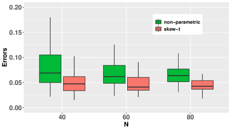
Figure 3: Errors of non-parametric and parametric approaches.

VI-B On Solving MVSK Portfolio Using RFPA Algorithm

In this subsection, we conduct experiments to evaluate how applying the ghMST distribution would accelerate the existing and proposed algorithms and the performance of our proposed RFPA algorithm on efficiency and scalability. We mainly utilize real-world data for the experiments. The data is randomly selected from the S&P 500 stock index. The trading period is chosen from 2011-01-01 to 2020-12-31.

VI-B1 Comparing non-parametric and parametric (ghMST) approach

We first perform the comparison on the non-parametric and parametric modeling of the high-order moments. Given the data, we first estimate the parameter $\boldsymbol{\Theta}$ for the ghMST distribution, then generate the sample moments, i.e., sample skewness matrix and kurtosis matrix, using Lemma 2. In this way, $\phi_{i}\left(\mathbf{w}\right)$, $i=1,2,3,4,$ will produce the same values under both non-parametric and parametric modeling.

We list the benchmarks as (first-order) MM algorithm [25], projected gradient descent (PGD) method, Q-MVSK (second-order SCA) algorithm [25], the nonlinear optimization solver ‘Nlopt’ [62] and our proposed RFPA algorithm. The inner solver for QP is selected as quadprog [63]. The weights $\boldsymbol{\lambda}$ are determined according to the Constant Relative Risk Aversion utility function

$$\boldsymbol{\lambda}^{T}=\left[1,\text{ }\frac{\xi}{2},\text{ }\frac{\xi\left(\xi+1\right)}{6},\text{ }\frac{\xi\left(\xi+1\right)\left(\xi+2\right)}{24}\right],$$ (56)

where $\xi\geq 0$ is a parameter to measure the risk aversion [64]. Suggested by [65, 66, 67], we set $\xi=6$ in this experiment. We further choose $\eta=5$, $\beta=0.5$ and investigate the empirical convergence of all algorithms under two different dimensions $N=100$ and $N=400$. The gap is defined as the difference of the objective value at each iteration and the smallest objective value we obtained across all the methods. When $N=400$, we cannot compare the performance of the non-parametric approaches due to the memory limit that renders them intractable.

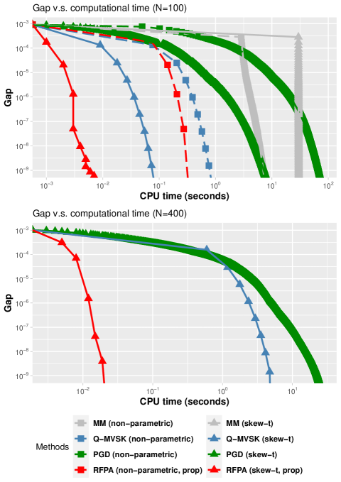
Figure 4: Convergence of algorithms for solving the MVSK portfolio optimization problems (6).

We have the following observations according to the simulation results exhibited in Figure 4. When $N=100$, the time cost for Nlopt (Non-parametric) and Nlopt (skew-$t$) is $9.349$ and $1.275$ seconds, respectively. When $N=400$, the number for Nlopt(skew-$t$) becomes $52.934$ seconds. Note that all the non-parametric approaches, which model the high-order moments using sample moments, are not applicable in high dimension due to the memory limit. Besides, MM methods require computing $\eta$ that meets the condition $\frac{1}{\eta}\geq\sup_{\mathbf{w}\in\mathcal{W}}\left\|\nabla f\left(\mathbf{w}\right)\right\|_{2}$, which is computationally expensive to obtain in high dimensional problems. From the numerical simulations we observe the following.

• By applying the parametric skew-$t$ distribution, we can accelerate the MVSK portfolio design by one-to-two orders of magnitude given any optimization algorithm when $N=100$.

• The per-iteration cost of proposed RFPA and PGD algorithms is significantly smaller than other methods with the help of water-filling algorithms.

• The effect of using the parametric skew-$t$ distribution tends to be algorithm-dependent. The acceleration is more noticeable for first-order algorithms like RFPA, which has negligible per-iteration cost.

VI-B2 Comparison on efficiency

To better compare the efficiency of the proposed algorithms, we also conduct experiments using real-world data sets with different problem dimensions. For each problem size, we set $\eta=5$, $\beta=0.5$, and take 200 independent experiments with $\xi$ randomly drawn from the interval $\left(10^{-1},10\right)$. All the methods are initialized with the same starting point $\mathbf{w}^{0}$. For Nlopt, the stopping criteria are set as the default. For Q-MVSK, PGD, and RFPA, the algorithms are regarded as converged when both the following conditions are satisfied:

$$\left|\mathbf{w}^{k+1}-\mathbf{w}^{k}\right|\leq 10^{-6}\left(\left|\mathbf{w}^{k+1}\right|+\left|\mathbf{w}^{k}\right|\right),$$ (57)

$$\left|f\left(\mathbf{w}^{k+1}\right)-f\left(\mathbf{w}^{k}\right)\right| \leq 10^{-6}\left(\left|f\left(\mathbf{w}^{k+1}\right)\right|+\left|f\left(\mathbf{w}^{k}\right)\right|\right).$$ (58)

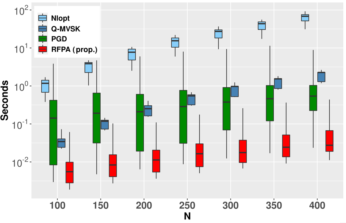
Figure 5: Comparison of algorithms with respect to the computational time under different data dimension.

According to the numerical simulation results shown in Figure 5, our proposed outperforms the state-of-the-art methods by one-to-two orders of magnitude when we assume the data follows a ghMST distribution. The difference seems to be enlarged when the problem dimension increases. Besides, the RFPA algorithm appears to be more stable compared to the PGD method.

VI-B3 Comparison on scalability

Interestingly, implied by Figure 5, first-order methods, including RFPA and PGD, appear to be more scalable than the second-order Q-MVSK algorithm. To better investigate this phenomenon, we will be conducting a comparison of these algorithms using a synthetic data set, where the parameter $\boldsymbol{\Theta}$ is randomly generated.

Table IV: Empirical orders of complexity.

Q-MVSK	Nlopt	PGD	RFPA
2.864	3.827	1.976	1.944

As shown in Figure 6, the proposed RFPA algorithm has a significantly lower complexity compared to the Q-MVSK algorithm, as its every single iteration does not contain procedures with high complexity. Meanwhile, PGD method also enjoys the benefits of low complexity but its overall efficiency is worse than the RFPA method. We also fit the empirical orders of the four methods considered. The relative results are shown in Table IV. It turns out that the empirical computational complexity of our method is $\mathcal{O}\left(N^{2}\right)$ and the complexity of the second-order method Q-MVSK is around $\mathcal{O}\left(N^{3}\right)$. The results of numerical simulations coincide with the discussion in Section IV-D.

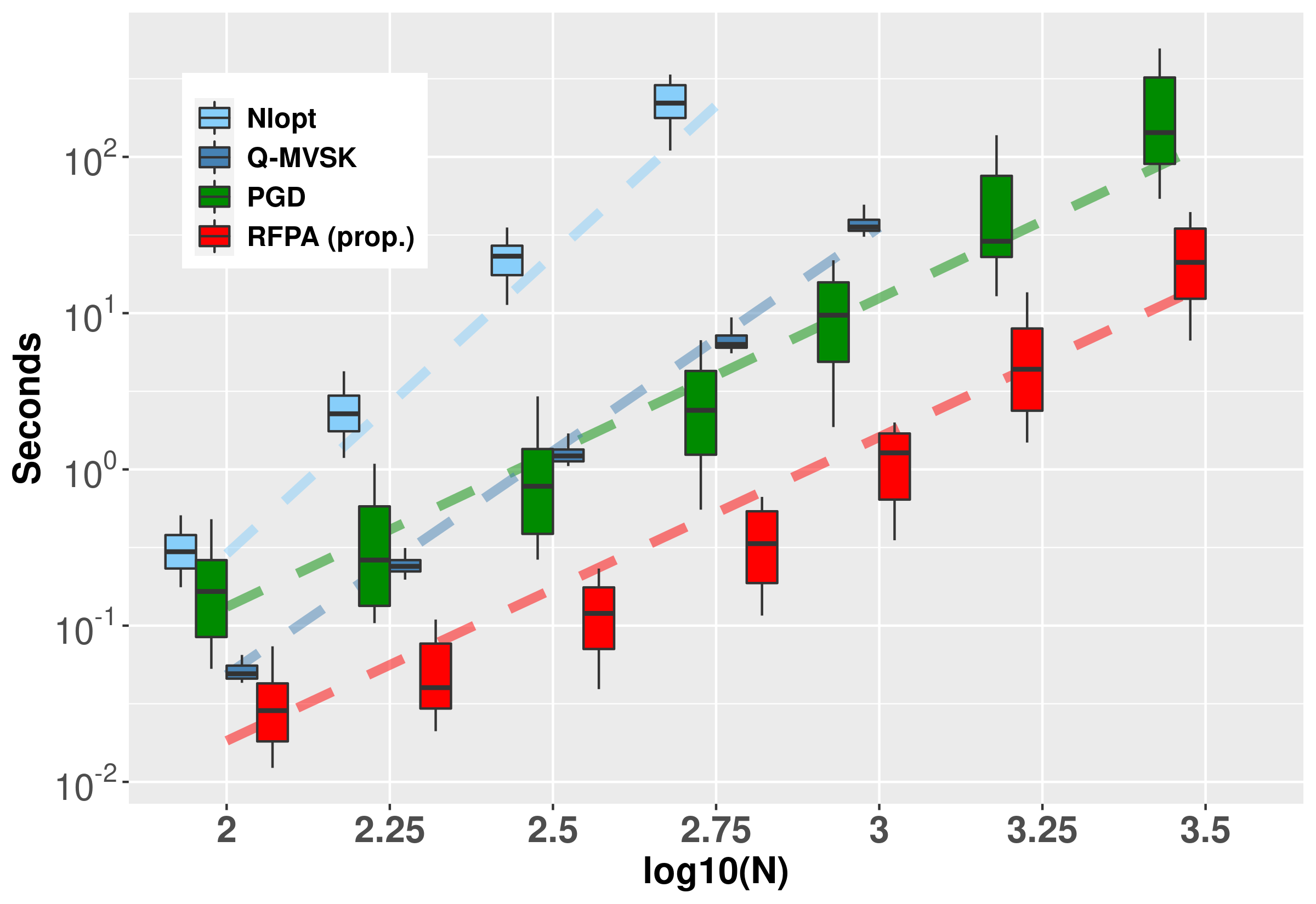
Figure 6: Investigation on the empirical complexity of RFPA and Q-MVSK algorithms.

VI-C Empirical Convergence of the proposed RFPA algorithm

According to Theorem 6, when $\mathbf{w}^{k}=\mathbf{w}^{k+1}$, the algorithm terminates at a stationary point of Problem (6). Though exact equality is often unattainable, empirically, the relative difference of $\mathbf{w}$, denoted as

$$\text{Relative Error}\left(\mathbf{w}^{k}\right)\overset{\Delta}{=}\left\|\mathbf{w}^{k}-\mathbf{w}^{k-1}\right\|\big{/}\left\|\mathbf{w}^{k}\right\|,$$ (59)

would tend to zero. To show this, we conduct experiments using real-world data sets with different problem dimensions. The values of (59) are computed at each iteration. From 7 we observe that the differences all reduce to very small numbers. Empirical studies show that the residual value $R\left(\mathbf{w}^{k};\eta\right)$ would tend to zero after $20$ iterations and the final solution would converge to the stationary point of Problem (6).

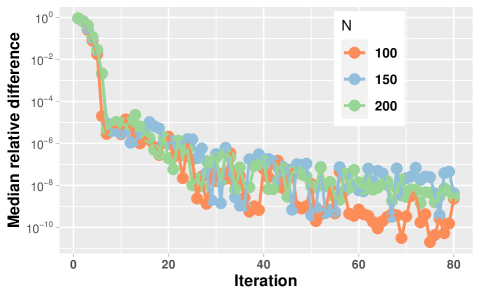
Figure 7: Median relative difference at each iteration.

VII Conclusion

In this paper, we have proposed a high-order portfolio design framework with the help of the parametric skew-$t$ distribution and a robust fixed point acceleration. The parametric approach is practical for modeling the skewness and kurtosis of portfolio returns in high-dimensional settings. By assuming the returns follow a ghMST distribution, we can alleviate the difficulties caused by the high complexity of traditional methods and accelerate all existing algorithms to a certain extent. Additionally, the proposed RFPA algorithm immensely cut down the number of iterations for first-order methods. Numerical simulations have demonstrated the outstanding efficiency and scalability of our proposed framework over the state-of-the-are benchmarks.

-A Computational time of different estimation methods

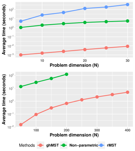
Figure 8: Comparing computational time (seconds) of different estimation methods.

Figure 8 depicts the computational time of different estimation methods. It can be observed that fitting the ghMST distribution is much more efficient than others.

-B Proof for Lemma 2

The proof starts with a fact that the central moments of a Gaussian variable $\tilde{\mathbf{X}}\sim\mathcal{N}\left(\tilde{\boldsymbol{\mu}},\tilde{\boldsymbol{\Sigma}}\right)$ is given by

$$\mathbb{E}[\tilde{X}_{i}] =\text{ }\tilde{\mu}_{i},$$ (60)

$$\mathbb{E}[\tilde{X}_{i}\tilde{X}_{j}] =\text{ }\tilde{\mu}_{i}\tilde{\mu}_{j}+\tilde{\Sigma}_{ij},$$

$$\mathbb{E}[\tilde{X}_{i}\tilde{X}_{j}\tilde{X}_{k}] =\text{ }\tilde{\mu}_{i}\tilde{\mu}_{j}\tilde{\mu}_{k}+\tilde{\mu}_{i}\tilde{\Sigma}_{jk}+\tilde{\mu}_{j}\tilde{\Sigma}_{ik}+\tilde{\mu}_{k}\tilde{\Sigma}_{ij},$$

$$\mathbb{E}[\tilde{X}_{i}\tilde{X}_{j}\tilde{X}_{k}\tilde{X}_{l}] =\text{ }\tilde{\mu}_{i}\tilde{\mu}_{j}\tilde{\mu}_{k}\tilde{\mu}_{l}+\underbrace{(\tilde{\Sigma}_{ij}\tilde{\mu}_{k}\tilde{\mu}_{l}+\cdots+\tilde{\Sigma}_{kl}\tilde{\mu}_{i}\tilde{\mu}_{j})}_{6\text{ items}}$$

$$\quad+(\tilde{\Sigma}_{ij}\tilde{\Sigma}_{kl}+\tilde{\Sigma}_{ik}\tilde{\Sigma}_{jl}+\tilde{\Sigma}_{il}\tilde{\Sigma}_{jk}).$$

Then, given the first term of the hierarchical structure $\mathbf{r}|\tau\overset{\text{i.i.d}}{\sim}\mathcal{N}\left(\boldsymbol{\mu}+\frac{1}{\tau}\boldsymbol{\gamma},\frac{1}{\tau}\boldsymbol{\Sigma}\right)$, we have

$$\mathbb{E}\left[r_{i}|\tau\right]=\mu_{i}+\frac{1}{\tau}\gamma_{i},$$ (61)

$$\mathbb{E}\left[r_{i}\right]=\mu_{i}+\mathbb{E}\left[\frac{1}{\tau}\right]\gamma_{i}=\mu_{i}+\frac{\nu}{\nu-2}\gamma_{i}.$$ (62)

Meanwhile, the hierarchical structure can be further written as

$$\mathbf{r}|\tau-\mathbb{E}\left[\mathbf{r}|\tau\right] \overset{\text{i.i.d}}{\sim}\,\,\mathcal{N}\left(\boldsymbol{\mu}+\frac{1}{\tau}\boldsymbol{\gamma}-\mathbb{E}\left[\mathbf{r}|\tau\right],\frac{1}{\tau}\boldsymbol{\Sigma}\right),$$ (63)

$$\tau \overset{\text{i.i.d}}{\sim}\,\,\text{Gamma}\left(\frac{\nu}{2},\frac{\nu}{2}\right),$$

where $\boldsymbol{\mu}+\frac{1}{\tau}\boldsymbol{\gamma}-\mathbb{E}\left[\mathbf{r}|\tau\right]=\left(\frac{1}{\tau}-\frac{\nu}{\nu-2}\right)\boldsymbol{\gamma}.$ Therefore, we can compute the central moments of $\tilde{\mathbf{r}}|\tau=\mathbf{r}|\tau-\mathbb{E}\left[\mathbf{r}|\tau\right]$ by regarding $\tilde{\boldsymbol{\mu}}=\left(\frac{1}{\tau}-\frac{\nu}{\nu-2}\right)\boldsymbol{\gamma}$ and $\tilde{\boldsymbol{\Sigma}}=\frac{1}{\tau}\boldsymbol{\Sigma}$:

$$\mathbb{E}[\left.\tilde{r}_{i}\tilde{r}_{j}\right|\tau] =\left(\frac{1}{\tau}-\frac{\nu}{\nu-2}\right)^{2}\gamma_{i}\gamma_{j}+\frac{1}{\tau}\Sigma_{ij},$$

$$\mathbb{E}[\left.\tilde{r}_{i}\tilde{r}_{j}\tilde{r}_{k}\right|\tau] =\left(\frac{1}{\tau}-\frac{\nu}{\nu-2}\right)^{3}\gamma_{i}\gamma_{j}\gamma_{k}+\frac{1}{\tau}\left(\frac{1}{\tau}-\frac{\nu}{\nu-2}\right)\cdot$$

$$\quad\quad\left[\gamma_{i}\Sigma_{jk}+\gamma_{j}\Sigma_{ik}+\gamma_{k}\Sigma_{ij}\right],$$

$$\mathbb{E}[\left.\tilde{r}_{i}\tilde{r}_{j}\tilde{r}_{k}\tilde{r}_{l}\right|\tau] =\left(\frac{1}{\tau}-\frac{\nu}{\nu-2}\right)^{4}\gamma_{i}\gamma_{j}\gamma_{k}\gamma_{l}+$$

$$\quad\left(\frac{1}{\tau}-\frac{\nu}{\nu-2}\right)^{2}\frac{1}{\tau}\cdot$$

$$\quad\underbrace{(\Sigma_{ij}\gamma_{k}\gamma_{l}+\cdots+\Sigma_{kl}\gamma_{i}\gamma_{j})}_{6\text{ items}}+$$

$$\quad\frac{1}{\tau^{2}}(\Sigma_{ij}\Sigma_{kl}+\Sigma_{ik}\Sigma_{jl}+\Sigma_{il}\Sigma_{jk}).$$ (64)

By taking expectation subject to $\tau$, i.e, $\mathbb{E}\left[\tau^{-1}\right]=\frac{\nu}{\nu-2}$, $\mathbb{E}\left[\tau^{-2}\right]=\frac{\nu^{2}}{\left(\nu-2\right)\left(\nu-4\right)},$$\mathbb{E}\left[\tau^{-3}\right]=\frac{\nu^{3}}{\left(\nu-2\right)\left(\nu-4\right)\left(\nu-6\right)}$, and $\mathbb{E}\left[\tau^{-4}\right]=\frac{\nu^{4}}{\left(\nu-2\right)\left(\nu-4\right)\left(\nu-6\right)\left(\nu-8\right)}$, the Lemma 2 is obtained.

-C Proof for Lemma 3

Assuming $\mathbf{r}\sim\textsf{ghMST}\left(\boldsymbol{\mu},\boldsymbol{\Sigma},\boldsymbol{\gamma},\nu\right)$, which indicates that the portfolio return $\mathbf{w}^{T}\mathbf{r}$ satisfies the following hierarchical structure:

$$\mathbf{w}^{T}\mathbf{r}|\tau \overset{\text{i.i.d}}{\sim}\,\,\mathcal{N}\left(\mathbf{w}^{T}\boldsymbol{\mu}+\frac{1}{\tau}\mathbf{w}^{T}\boldsymbol{\gamma},\frac{1}{\tau}\mathbf{w}^{T}\boldsymbol{\Sigma}\mathbf{w}\right),$$ (65)

$$\tau \overset{\text{i.i.d}}{\sim}\,\,\text{Gamma}\left(\frac{\nu}{2},\frac{\nu}{2}\right),$$

Then, according to (65), we have

$$\mathbf{w}^{T}\mathbf{r}\sim\text{{ghMST}$\left(\mathbf{w}^{T}\boldsymbol{\mu},\mathbf{w}^{T}\boldsymbol{\Sigma}\mathbf{w},\mathbf{w}^{T}\boldsymbol{\gamma},\nu\right)$}.$$ (66)

As $\mathbf{w}^{T}\mathbf{r}$ is a scalar, its high-order central moments, i.e., $\boldsymbol{\Phi}$ and $\boldsymbol{\Psi}$ are all scalars. Based on Lemma 2, we replace $\boldsymbol{\mu}$, $\boldsymbol{\Sigma}$, and $\boldsymbol{\gamma}$ with $\mathbf{w}^{T}\boldsymbol{\mu},\mathbf{w}^{T}\boldsymbol{\Sigma}\mathbf{w}$, and $\mathbf{w}^{T}\boldsymbol{\gamma}$, respectively. Then we can obtain

$$\phi_{3}\left(\mathbf{w}\right) =\Phi=\mathbb{E}\left[\left(\frac{1}{\tau}-\frac{\nu}{\nu-2}\right)^{3}\right]\left(\mathbf{w}^{T}\boldsymbol{\gamma}\right)^{3}+$$

$$\quad\quad 3\mathbb{E}\left[\frac{1}{\tau}\left(\frac{1}{\tau}-\frac{\nu}{\nu-2}\right)\right]\left(\mathbf{w}^{T}\boldsymbol{\Sigma}\mathbf{w}\cdot\mathbf{w}^{T}\boldsymbol{\gamma}\right),$$

$$\phi_{4}\left(\mathbf{w}\right) =\Psi=\mathbb{E}\left[\left(\frac{1}{\tau}-\frac{\nu}{\nu-2}\right)^{4}\right]\left(\mathbf{w}^{T}\boldsymbol{\gamma}\right)^{4}$$

$$\quad\quad+6\mathbb{E}\left[\left(\frac{1}{\tau}-\frac{\nu}{\nu-2}\right)^{2}\right]\left(\mathbf{w}^{T}\boldsymbol{\gamma}\right)^{2}\left(\mathbf{w}^{T}\boldsymbol{\Sigma}\mathbf{w}\right)$$

$$\quad\quad+3\mathbb{E}\left[\frac{1}{\tau^{2}}\right]a_{43}\left(\mathbf{w}^{T}\boldsymbol{\Sigma}\mathbf{w}\right)^{2}.$$ (67)

Simply follows the definition of $\mathbf{a}$, Lemma 3 is proved.

-D Gradient and Hessian of the high-order moments

Based on Lemma 3, the gradient and Hessian of the skewness and kurtosis subject to $\mathbf{w}$ can be computed as

$$\begin{array}[]{rl}\nabla\phi_{3}\left(\mathbf{w}\right)=&3a_{31}\left(\mathbf{w}^{T}\boldsymbol{\gamma}\right)^{2}\boldsymbol{\gamma}\\ &+a_{32}\left[\left(\mathbf{w}^{T}\boldsymbol{\Sigma}\mathbf{w}\right)\boldsymbol{\gamma}+2\left(\mathbf{w}^{T}\boldsymbol{\gamma}\right)\boldsymbol{\Sigma}\mathbf{w}\right],\\ \nabla^{2}\phi_{3}\left(\mathbf{w}\right)=&6a_{31}\left(\mathbf{w}^{T}\boldsymbol{\gamma}\right)\boldsymbol{\gamma}\boldsymbol{\gamma}^{T}\\ &+2a_{32}\left[\boldsymbol{\gamma}\mathbf{w}^{T}\boldsymbol{\Sigma}+\boldsymbol{\Sigma}\mathbf{w}\boldsymbol{\gamma}^{T}+\mathbf{w}^{T}\boldsymbol{\gamma}\boldsymbol{\Sigma}\right],\\ \nabla\phi_{4}\left(\mathbf{w}\right)=&4a_{41}\left(\mathbf{w}^{T}\boldsymbol{\gamma}\right)^{3}\boldsymbol{\gamma}\\ &+2a_{42}\left[\left(\mathbf{w}^{T}\boldsymbol{\gamma}\right)^{2}\boldsymbol{\Sigma}\mathbf{w}+\left(\mathbf{w}^{T}\boldsymbol{\Sigma}\mathbf{w}\right)\left(\mathbf{w}^{T}\boldsymbol{\gamma}\right)\boldsymbol{\gamma}\right]\\ &+4a_{43}\left(\mathbf{w}^{T}\boldsymbol{\Sigma}\mathbf{w}\right)\boldsymbol{\Sigma}\mathbf{w},\\ \nabla^{2}\phi_{4}\left(\mathbf{w}\right)=&12a_{41}\left(\mathbf{w}^{T}\boldsymbol{\gamma}\right)^{2}\boldsymbol{\gamma}\boldsymbol{\gamma}^{T}\\ &+2a_{42}\left[2\left(\mathbf{w}^{T}\boldsymbol{\gamma}\right)\boldsymbol{\Sigma}\mathbf{w}\boldsymbol{\gamma}^{T}+\left(\mathbf{w}^{T}\boldsymbol{\gamma}\right)^{2}\boldsymbol{\Sigma}+\right.\\ &\quad\quad\left.2\left(\mathbf{w}^{T}\boldsymbol{\gamma}\right)\boldsymbol{\gamma}\mathbf{w}^{T}\boldsymbol{\Sigma}+\left(\mathbf{w}^{T}\boldsymbol{\Sigma}\mathbf{w}\right)\boldsymbol{\gamma}\boldsymbol{\gamma}^{T}\right]\\ &+4a_{43}\left[2\boldsymbol{\Sigma}\mathbf{w}\mathbf{w}^{T}\boldsymbol{\Sigma}+\left(\mathbf{w}^{T}\boldsymbol{\Sigma}\mathbf{w}\right)\boldsymbol{\Sigma}\right].\end{array}$$ (68)

-E Water-filling algorithm

Here we consider an optimization problem

$$\begin{array}[]{ll}\underset{\mathbf{w}}{\mathsf{minimize}}&\frac{1}{2}\left\|\mathbf{w}-\left(\mathbf{w}^{k}-\eta\nabla f\left(\mathbf{w}^{k}\right)\right)\right\|_{2}^{2}\\ \mathsf{subject}\text{ }\mathsf{to}&\mathbf{w}\in\mathcal{W}.\end{array}$$ (69)

Given $\mathcal{W}=\left\{\mathbf{w}\left|\mathbf{1}^{T}\mathbf{w}=1,\mathbf{w}\geq\mathbf{0}\right.\right\}$, the Lagrangian of Problem (69) is

$$\mathcal{L}\left(\mathbf{w},\boldsymbol{\psi},\gamma\right) =\frac{1}{2}\left\|\mathbf{w}-\left(\mathbf{w}^{k}-\eta\nabla f\left(\mathbf{w}^{k}\right)\right)\right\|_{2}^{2}$$

$$\quad-\boldsymbol{\psi}^{T}\mathbf{w}+\gamma\left(\mathbf{1}^{T}\mathbf{w}-1\right),$$ (70)

where $\boldsymbol{\psi}$ and $\gamma$ are dual variables associated with the constraints $\mathbf{w}\geq\mathbf{0}$ and $\mathbf{1}^{T}\mathbf{w}=1$, respectively. The KKT conditions are

$$\eta\nabla f\left(\mathbf{w}^{k}\right)+\left(\mathbf{w}-\mathbf{w}^{k}\right)-\boldsymbol{\psi}+\gamma\mathbf{1} =\mathbf{0},$$

$$\boldsymbol{\psi}\odot\mathbf{w} =\mathbf{0}.$$ (71)

Hence, we have

$$w_{i}=\max\left(0,w_{i}^{k}-\eta\left[\nabla f\left(\mathbf{w}^{k}\right)\right]_{i}-\gamma\right).$$ (72)

Define a continuous and monotone decreasing function $\zeta:\mathbb{R}\rightarrow\mathbb{R}$:

$$\zeta\left(\gamma\right)=\sum_{i=1}^{N}\max\left(0,w_{i}^{k}-\eta\left[\nabla f\left(\mathbf{w}^{k}\right)\right]_{i}-\gamma\right)-1$$ (73)

with $\zeta\left(-\infty\right)=+\infty$ and $\zeta\left(-\infty\right)=-1$, the root

$$\gamma^{\star}=\arg\left(\zeta\left(\gamma\right)=0\right)$$ (74)

exists and is unique. The root provides a dual optimal of the KKT system. We can easily solve $\gamma$ and $\mathbf{w}^{\star}$ via bisection.

-F Monotonicity of the sequence $\left\{f\left(\mathbf{w}^{k}\right)\right\}$

According to the projection theorem [68], i.e.,

$$\forall\mathbf{x},\mathbf{z}:\left\langle\mathbf{z}-\mathbf{x},\mathcal{P}_{\mathcal{W}}\left(\mathbf{z}\right)-\mathcal{P}_{\mathcal{W}}\left(\mathbf{x}\right)\right\rangle\geq\left\|\mathcal{P}_{\mathcal{W}}\left(\mathbf{z}\right)-\mathcal{P}_{\mathcal{W}}\left(\mathbf{x}\right)\right\|_{2}^{2},$$ (75)

we apply $\mathbf{z}=\mathbf{w}^{k}-\eta\nabla f\left(\mathbf{w}^{k}\right)$ and $\mathbf{x}=\mathbf{w}^{k}$ to obtain

$$\left\langle-\eta\nabla f\left(\mathbf{w}^{k}\right),\mathbf{w}^{k+1}-\mathbf{w}^{k}\right\rangle\geq\left\|\mathbf{w}^{k+1}-\mathbf{w}^{k}\right\|_{2}^{2},$$ (76)

or equivalently

$$\left\langle\nabla f\left(\mathbf{w}^{k}\right),\mathbf{w}^{k+1}-\mathbf{w}^{k}\right\rangle\leq-\frac{1}{\eta}\left\|\mathbf{w}^{k+1}-\mathbf{w}^{k}\right\|_{2}^{2}.$$ (77)

Hence, from the inequality (41) we have

$$f\left(\mathbf{w}^{k+1}\right) \leq f\left(\mathbf{w}^{k}\right)+\nabla f\left(\mathbf{w}^{k}\right)^{T}\left(\mathbf{w}^{k+1}-\mathbf{w}^{k}\right)$$

$$\quad+\frac{1}{2\eta}\left\|\mathbf{w}^{k}-\mathbf{w}^{k+1}\right\|_{2}^{2}$$

$$\leq f\left(\mathbf{w}^{k}\right)-\frac{1}{\eta}\left\|\mathbf{w}^{k+1}-\mathbf{w}^{k}\right\|_{2}^{2}$$

$$\quad+\frac{1}{2\eta}\left\|\mathbf{w}^{k}-\mathbf{w}^{k+1}\right\|_{2}^{2}$$

$$=f\left(\mathbf{w}^{k}\right)-\frac{1}{2\eta}\left\|\mathbf{w}^{k}-\mathbf{w}^{k+1}\right\|_{2}^{2}\leq f\left(\mathbf{w}^{k}\right),$$ (78)

which indicates that the sequence $\left\{f\left(\mathbf{w}^{k}\right)\right\}$ is then monotone.

-G Proof of Theorem 6

Proof:

When $\mathbf{w}^{k}=\mathbf{w}^{k+1}$, we may have $\mathbf{w}^{k+1}=\mathcal{P}_{\mathcal{W}}\left(\mathbf{w}^{k}-2\alpha^{k}R\left(\mathbf{w}^{k};\eta\right)+\left(\alpha^{k}\right)^{2}V\left(\mathbf{w}^{k};\eta\right)\right)$ or $\mathbf{w}^{k+1}=G\left(\mathbf{w}^{k};\eta^{\prime}\right)$.

(i) We first analyze the first case where $\mathbf{w}^{k+1}=\mathcal{P}_{\mathcal{W}}\left(\mathbf{y}^{k}\right)$, in which

$$\mathbf{y}^{k}\overset{\Delta}{=}\mathbf{w}^{k}-2\alpha^{k}R\left(\mathbf{w}^{k};\eta\right)+\left(\alpha^{k}\right)^{2}V\left(\mathbf{w}^{k};\eta\right).$$ (79)

By applying the contraposition, we prove the following statement instead

$$\forall\mathbf{w}^{k}\in\mathcal{W}:R\left(\mathbf{w}^{k};\eta\right)\neq\mathbf{0}\Rightarrow\mathcal{P}_{\mathcal{W}}\left(\mathbf{y}^{k}\right)\neq\mathbf{w}^{k}.$$ (80)

For simplicity, we denote $\alpha=-\alpha^{k}>0$. Note that $\alpha\neq 0$ as $R\left(\mathbf{w}^{k};\eta\right)\neq\mathbf{0}$.

(A) If $\alpha\in\left(0,1\right]$, then, we obtain

$$\mathbf{y}^{k} =\left(1-2\alpha+\alpha^{2}\right)\mathbf{w}^{k}+\left(2\alpha-2\alpha^{2}\right)G\left(\mathbf{w}^{k};\eta\right)$$

$$\quad+\alpha^{2}G\left(G\left(\mathbf{w}^{k};\eta\right);\eta\right)$$

$$\overset{\Delta}{=}a^{k}\mathbf{w}^{k}+b^{k}G\left(\mathbf{w}^{k};\eta\right)+c^{k}G\left(G\left(\mathbf{w}^{k};\eta\right);\eta\right)$$ (81)

in which $a^{k}=1-2\alpha+\alpha^{2}$, $b^{k}=2\alpha-2\alpha^{2}$, and $c^{k}=\alpha^{2}$. As $0<\alpha\leq 1$, we have $0\leq a^{k}<1$, $0\leq b^{k}\leq\frac{1}{2}$, $0<c^{k}\leq 1$, and $a^{k}+b^{k}+c^{k}=1$. Hence, $\mathbf{y}^{k}$ is a convex combination of $\mathbf{w}^{k}$, $G\left(\mathbf{w}^{k};\eta\right)$, and $G\left(G\left(\mathbf{w}^{k};\eta\right);\eta\right)$. As a result, $\mathbf{y}^{k}\in\mathcal{W}$ and the projection of $\mathbf{y}^{k}$ onto $\mathcal{W}$ is itself, i.e., $\mathcal{P}_{\mathcal{W}}\left(\mathbf{y}^{k}\right)=\mathbf{y}^{k}$. Consequently, we obtain

$$\mathbf{w}^{k+1}=\mathcal{P}_{\mathcal{W}}\left(\mathbf{y}^{k}\right)\neq\mathbf{w}^{k}.$$ (82)

(B) If $\alpha\in\left(1,\infty\right)$. We will first show that the following inequality holds for any $\mathbf{w}^{k}$

$$\xi\overset{\Delta}{=}\left\langle R\left(\mathbf{w}^{k};\eta\right),R\left(\mathbf{w}^{k};\eta\right)+\alpha V\left(\mathbf{w}^{k};\eta\right)\right\rangle\geq 0.$$ (83)

In principle, we consider the following three cases based on the value of $\left\langle R\left(\mathbf{w}^{k};\eta\right),V\left(\mathbf{w}^{k};\eta\right)\right\rangle$.

(B.1) If $\left\langle R\left(\mathbf{w}^{k};\eta\right),V\left(\mathbf{w}^{k};\eta\right)\right\rangle\geq 0$, then $b\left(\mathbf{w}^{k}\right)=-\infty$. (83) holds as $\forall\alpha>1$:

$$\xi=\left\|R\left(\mathbf{w}^{k};\eta\right)\right\|^{2}+\alpha\left\langle R\left(\mathbf{w}^{k};\eta\right),V\left(\mathbf{w}^{k};\eta\right)\right\rangle\geq 0.$$ (84)

(B.2) If $\left\langle R\left(\mathbf{w}^{k};\eta\right),V\left(\mathbf{w}^{k};\eta\right)\right\rangle<0$ and $b\left(\mathbf{w}^{k}\right)=\frac{\left\|R\left(\mathbf{w}^{k};\eta\right)\right\|_{2}^{2}}{\left\langle R\left(\mathbf{w}^{k};\eta\right),V\left(\mathbf{w}^{k};\eta\right)\right\rangle}\neq-\infty$, we have $\alpha\leq-b\left(\mathbf{w}^{k}\right)$. In this case, (83) holds as $\forall\alpha\in\left(1,-b\left(\mathbf{w}^{k}\right)\right)$:

$$\xi= \left\|R\left(\mathbf{w}^{k};\eta\right)\right\|^{2}+\alpha\left\langle R\left(\mathbf{w}^{k};\eta\right),V\left(\mathbf{w}^{k};\eta\right)\right\rangle$$

$$\geq \left\|R\left(\mathbf{w}^{k};\eta\right)\right\|^{2}-b\left(\mathbf{w}^{k}\right)\left\langle R\left(\mathbf{w}^{k};\eta\right),V\left(\mathbf{w}^{k};\eta\right)\right\rangle=0.$$ (85)

(B.3) If $\left\langle R\left(\mathbf{w}^{k};\eta\right),V\left(\mathbf{w}^{k};\eta\right)\right\rangle<0$ but $b\left(\mathbf{w}^{k}\right)\rightarrow-\infty$ due to $V\left(\mathbf{w}^{k};\eta\right)\rightarrow\mathbf{0}$, the value of $\alpha$ can be either $\left\|R\left(\mathbf{w}^{k};\eta\right)\right\|\big{/}\left\|V\left(\mathbf{w}^{k};\eta\right)\right\|\rightarrow\infty$ or $-b\left(\mathbf{w}^{k}\right)\rightarrow\infty$. When $\alpha=\left\|R\left(\mathbf{w}^{k};\eta\right)\right\|\big{/}\left\|V\left(\mathbf{w}^{k};\eta\right)\right\|$, we suppose

$$\left\langle R\left(\mathbf{w}^{k};\eta\right),V\left(\mathbf{w}^{k};\eta\right)\right\rangle$$

$$= \left\|R\left(\mathbf{w}^{k};\eta\right)\right\|\left\|V\left(\mathbf{w}^{k};\eta\right)\right\|\cos\theta_{R,V},$$ (86)

in which $\theta_{R,V}$ is the angle between $R\left(\mathbf{w}^{k};\eta\right)$ and $V\left(\mathbf{w}^{k};\eta\right)$. Hence, as $\cos\theta_{R,V}\in\left[-1,1\right]$, we obtain

$$\xi =\left\|R\left(\mathbf{w}^{k};\eta\right)\right\|^{2}+\frac{\left\|R\left(\mathbf{w}^{k};\eta\right)\right\|}{\left\|V\left(\mathbf{w}^{k};\eta\right)\right\|}\left\langle R\left(\mathbf{w}^{k};\eta\right),V\left(\mathbf{w}^{k};\eta\right)\right\rangle$$

$$=\left\|R\left(\mathbf{w}^{k};\eta\right)\right\|^{2}\left(1+\cos\theta_{R,V}\right)\geq 0.$$ (87)

When $\alpha=-b\left(\mathbf{w}^{k}\right)=-\frac{\left\|R\left(\mathbf{w}^{k};\eta\right)\right\|_{2}^{2}}{\left\langle R\left(\mathbf{w}^{k};\eta\right),V\left(\mathbf{w}^{k};\eta\right)\right\rangle}$, it is obvious that

$$\xi=\left\|R\left(\mathbf{w}^{k};\eta\right)\right\|^{2}-b\left(\mathbf{w}^{k}\right)\left\langle R\left(\mathbf{w}^{k};\eta\right),V\left(\mathbf{w}^{k};\eta\right)\right\rangle=0.$$ (88)

Therefore, (83) holds. As a consequence, we can compare the following two terms

$$\mathbf{y}^{k}-\mathbf{w}^{k} =\alpha R\left(\mathbf{w}^{k};\eta\right)$$

$$\quad+\alpha\left(R\left(\mathbf{w}^{k};\eta\right)+\alpha V\left(\mathbf{w}^{k};\eta\right)\right),$$

$$\mathbf{y}^{k}-G\left(\mathbf{w}^{k};\eta\right) =\left(\alpha-1\right)R\left(\mathbf{w}^{k};\eta\right)$$

$$\quad+\alpha\left(R\left(\mathbf{w}^{k};\eta\right)+\alpha V\left(\mathbf{w}^{k};\eta\right)\right),$$ (89)

by evaluating the difference of their squared $\ell_{2}$ norms, i.e.,

$$\left\|\mathbf{y}^{k}-\mathbf{w}^{k}\right\|^{2}-\left\|\mathbf{y}^{k}-G\left(\mathbf{w}^{k};\eta\right)\right\|^{2}$$

$$= \left(2\alpha-1\right)\left\|R\left(\mathbf{w}^{k};\eta\right)\right\|^{2}$$

$$\quad+2\alpha\left\langle R\left(\mathbf{w}^{k};\eta\right),R\left(\mathbf{w}^{k};\eta\right)+\alpha V\left(\mathbf{w}^{k};\eta\right)\right\rangle.$$ (90)

Then, we obtain the following strict inequality

$$\left\|\mathbf{y}^{k}-\mathbf{w}^{k}\right\|^{2}-\left\|\mathbf{y}^{k}-G\left(\mathbf{w}^{k};\eta\right)\right\|^{2}>0$$ (91)

as $\alpha>1$ and $\left\|R\left(\mathbf{w}^{k};\eta\right)\right\|>0$. Therefore, $\mathcal{P}_{\mathcal{W}}\left(\mathbf{y}^{k}\right)\neq\mathbf{w}^{k}$ as there exists a feasible point $G\left(\mathbf{w}^{k};\eta\right)\in\mathcal{W}$ that is closer to $\mathbf{y}^{k}$ compared to $\mathbf{w}^{k}$.

Hence, we have shown that $\mathcal{P}_{\mathcal{W}}\left(\mathbf{y}^{k}\right)\neq\mathbf{w}^{k}$ if $R\left(\mathbf{w}^{k};\eta\right)\neq\mathbf{0}$. As a result, we have obtained the following statement

$$\mathcal{P}_{\mathcal{W}}\left(\mathbf{y}^{k}\right)=\mathbf{w}^{k}\Rightarrow R\left(\mathbf{w}^{k};\eta\right)=\mathbf{0}.$$ (92)

Then, $\mathbf{w}^{k}$ is a stationary point of Problem (6) according to Lemma 5.

(ii) We then analyze the second case where

$$\mathbf{w}^{k+1}=\mathcal{P}_{\mathcal{W}}\left(\mathbf{w}^{k}-\eta^{\prime}\nabla f\left(\mathbf{w}^{k}\right)\right).$$ (93)

Then, $\mathbf{w}^{k}$ is a stationary point of Problem (6) when $\mathbf{w}^{k+1}=\mathbf{w}^{k}$ with the proof directly from [69, Theorem 9.10].

In conclusion, once we obtain $\mathbf{w}^{k+1}=\mathbf{w}^{k}$ from the proposed RFPA algorithm, $\mathbf{w}^{k}$ is a stationary point of Problem (6). ∎

References

- [1] H. M. Markowitz, “Portfolio Selection,” Journal of Finance, vol. 7, no. 1, pp. 77–91, 1952.
- [2] ——, “Foundations of portfolio theory,” The Journal of Finance, vol. 46, no. 2, pp. 469–477, 1991.
- [3] C. Adcock, M. Eling, and N. Loperfido, “Skewed distributions in finance and actuarial science: a review,” The European Journal of Finance, vol. 21, no. 13-14, pp. 1253–1281, 2015.
- [4] S. I. Resnick, Heavy-tail phenomena: probabilistic and statistical modeling. Springer Science & Business Media, 2007.
- [5] P. N. Kolm, R. Tütüncü, and F. J. Fabozzi, “60 years of portfolio optimization: Practical challenges and current trends,” European Journal of Operational Research, vol. 234, no. 2, pp. 356–371, 2014.
- [6] J. V. de M. Cardoso, J. Ying, and D. P. Palomar, “Graphical models in heavy-tailed markets,” Advances in Neural Information Processing Systems, vol. 34, pp. 19 989–20 001, 2021.
- [7] E. Jondeau and M. Rockinger, “Conditional volatility, skewness, and kurtosis: existence, persistence, and comovements,” Journal of Economic Dynamics and Control, vol. 27, no. 10, pp. 1699–1737, 2003.
- [8] J. V. de M. Cardoso, J. Ying, and D. P. Palomar, “Learning bipartite graphs: Heavy tails and multiple components,” Advances in Neural Information Processing Systems, vol. 35, pp. 14 044–14 057, 2022.
- [9] B. O. Bradley and M. S. Taqqu, “Financial risk and heavy tails,” in Handbook of Heavy Tailed Distributions in Finance. Elsevier, 2003, pp. 35–103.
- [10] J. V. Rosenberg and T. Schuermann, “A general approach to integrated risk management with skewed, fat-tailed risks,” Journal of Financial Economics, vol. 79, no. 3, pp. 569–614, 2006.
- [11] K. Gaurav and P. Mohanty, “Effect of skewness on optimum portfolio selection,” IUP Journal of Applied Finance, vol. 19, no. 3, p. 56, 2013.
- [12] D. Maringer and P. Parpas, “Global optimization of higher order moments in portfolio selection,” Journal of Global Optimization, vol. 43, no. 2, pp. 219–230, 2009.
- [13] R. C. Scott and P. A. Horvath, “On the direction of preference for moments of higher order than the variance,” The Journal of Finance, vol. 35, no. 4, pp. 915–919, 1980.
- [14] L. T. DeCarlo, “On the meaning and use of kurtosis.” Psychological Methods, vol. 2, no. 3, p. 292, 1997.
- [15] E. Jondeau and M. Rockinger, “Optimal portfolio allocation under higher moments,” European Financial Management, vol. 12, no. 1, pp. 29–55, 2006.
- [16] C. R. Harvey, J. C. Liechty, M. W. Liechty, and P. Müller, “Portfolio selection with higher moments,” Quantitative Finance, vol. 10, no. 5, pp. 469–485, 2010.
- [17] J. He, Q.-G. Wang, P. Cheng, J. Chen, and Y. Sun, “Multi-period mean-variance portfolio optimization with high-order coupled asset dynamics,” IEEE Transactions on Automatic Control, vol. 60, no. 5, pp. 1320–1335, 2014.
- [18] L. Martellini and V. Ziemann, “Improved estimates of higher-order comoments and implications for portfolio selection,” The Review of Financial Studies, vol. 23, no. 4, pp. 1467–1502, 2010.
- [19] E. Jondeau, “Asymmetry in tail dependence in equity portfolios,” Computational Statistics & Data Analysis, vol. 100, pp. 351–368, 2016.
- [20] S. Liu, P.-Y. Chen, B. Kailkhura, G. Zhang, A. O. Hero III, and P. K. Varshney, “A primer on zeroth-order optimization in signal processing and machine learning: Principals, recent advances, and applications,” IEEE Signal Processing Magazine, vol. 37, no. 5, pp. 43–54, 2020.
- [21] B. Babu and M. M. L. Jehan, “Differential evolution for multi-objective optimization,” in The 2003 Congress on Evolutionary Computation, 2003. CEC’03., vol. 4. IEEE, 2003, pp. 2696–2703.
- [22] S. Kshatriya and P. K. Prasanna, “Genetic algorithm-based portfolio optimization with higher moments in global stock markets,” Journal of Risk, vol. 20, no. 4, 2018.
- [23] T. P. Dinh and Y.-S. Niu, “An efficient DC programming approach for portfolio decision with higher moments,” Computational Optimization and Applications, vol. 50, no. 3, pp. 525–554, 2011.
- [24] Y.-S. Niu and Y.-J. Wang, “Higher-order moment portfolio optimization via the difference-of-convex programming and sums-of-squares,” arXiv preprint arXiv:1906.01509, 2019.
- [25] R. Zhou and D. P. Palomar, “Solving high-order portfolios via successive convex approximation algorithms,” IEEE Transactions on Signal Processing, vol. 69, pp. 892–904, 2021.
- [26] K. Aas and I. H. Haff, “The generalized hyperbolic skew Students’t-distribution,” Journal of Financial Econometrics, vol. 4, no. 2, pp. 275–309, 2006.
- [27] Y. Wei, Y. Tang, and P. D. McNicholas, “Mixtures of generalized hyperbolic distributions and mixtures of skew-t distributions for model-based clustering with incomplete data,” Computational Statistics & Data Analysis, vol. 130, pp. 18–41, 2019.
- [28] O. Barndorff-Nielsen, “Exponentially decreasing distributions for the logarithm of particle size,” Proceedings of the Royal Society of London. A. Mathematical and Physical Sciences, vol. 353, no. 1674, pp. 401–419, 1977.
- [29] M. Hellmich and S. Kassberger, “Efficient and robust portfolio optimization in the multivariate generalized hyperbolic framework,” Quantitative Finance, vol. 11, no. 10, pp. 1503–1516, 2011.
- [30] W. Hu and A. Kercheval, “Risk management with generalized hyperbolic distributions,” in Proceedings of the Fourth IASTED International Conference on Financial Engineering and Applications. ACTA Press, 2007, pp. 19–24.
- [31] J. R. Birge and L. Chavez-Bedoya, “Portfolio optimization under a generalized hyperbolic skewed-t distribution and exponential utility,” Quantitative Finance, vol. 16, no. 7, pp. 1019–1036, 2016.
- [32] M. Haas and C. Pigorsch, “Financial economics, fat-tailed distributions.” Encyclopedia of Complexity and Systems Science, vol. 4, no. 1, pp. 3404–3435, 2009.
- [33] O. E. Barndorff-Nielsen, T. Mikosch, and S. I. Resnick, Lévy processes: theory and applications. Springer Science & Business Media, 2012.
- [34] A. Gupta, “Multivariate skew t-distribution,” Statistics: A Journal of Theoretical and Applied Statistics, vol. 37, no. 4, pp. 359–363, 2003.
- [35] S. Pyne, X. Hu, K. Wang, E. Rossin, T.-I. Lin, L. M. Maier, C. Baecher-Allan, G. J. McLachlan, P. Tamayo, D. A. Hafler et al., “Automated high-dimensional flow cytometric data analysis,” Proceedings of the National Academy of Sciences, vol. 106, no. 21, pp. 8519–8524, 2009.
- [36] M. D. Branco and D. K. Dey, “A general class of multivariate skew-elliptical distributions,” Journal of Multivariate Analysis, vol. 79, no. 1, pp. 99–113, 2001.
- [37] A. Azzalini and A. Capitanio, “Distributions generated by perturbation of symmetry with emphasis on a multivariate skew t-distribution,” Journal of the Royal Statistical Society: Series B (Statistical Methodology), vol. 65, no. 2, pp. 367–389, 2003.
- [38] S. X. Lee and G. J. McLachlan, “On mixtures of skew normal and skew-t distributions,” Advances in Data Analysis and Classification, vol. 7, no. 3, pp. 241–266, 2013.
- [39] S. K. Sahu, D. K. Dey, and M. D. Branco, “A new class of multivariate skew distributions with applications to Bayesian regression models,” Canadian Journal of Statistics, vol. 31, no. 2, pp. 129–150, 2003.
- [40] S. Lee and G. J. McLachlan, “Finite mixtures of multivariate skew-t distributions: some recent and new results,” Statistics and Computing, vol. 24, no. 2, pp. 181–202, 2014.
- [41] K. Wang, S.-K. Ng, and G. J. McLachlan, “Multivariate skew t mixture models: applications to fluorescence-activated cell sorting data,” in 2009 Digital Image Computing: Techniques and Applications. IEEE, 2009, pp. 526–531.
- [42] K. Wang, A. Ng, G. McLachlan, and M. S. Lee, “Package ’EMMIXskew’,” 2018.
- [43] D. P. Palomar, R. Zhou, X. Wang, F. Pascal, and E. Ollila, “fitHeavyTail: Mean and covariance matrix estimation under heavy tails, 2020, R package version 0.1. 2.”
- [44] W. Breymann and D. Lüthi, “ghyp: A package on generalized hyperbolic distributions,” Manual for R Package ghyp, 2013.
- [45] A. J. McNeil, R. Frey, and P. Embrechts, Quantitative risk management: concepts, techniques and tools-revised edition. Princeton university press, 2015.
- [46] L. Condat, “Fast projection onto the simplex and the ball,” Mathematical Programming, vol. 158, no. 1, pp. 575–585, 2016.
- [47] D. P. Palomar and J. R. Fonollosa, “Practical algorithms for a family of waterfilling solutions,” IEEE Transactions on Signal Processing, vol. 53, no. 2, pp. 686–695, 2005.
- [48] K. L. Judd, Numerical methods in economics. MIT press, 1998.
- [49] L. Qi and J. Sun, “A nonsmooth version of Newton’s method,” Mathematical Programming, vol. 58, no. 1, pp. 353–367, 1993.
- [50] F. H. Clarke, Optimization and nonsmooth analysis. SIAM, 1990.
- [51] R. Varadhan and C. Roland, “Squared extrapolation methods (SQUAREM): A new class of simple and efficient numerical schemes for accelerating the convergence of the EM algorithm,” 2004.
- [52] M. Raydan and B. F. Svaiter, “Relaxed steepest descent and cauchy-barzilai-borwein method,” Computational Optimization and Applications, vol. 21, no. 2, pp. 155–167, 2002.
- [53] R. Varadhan and C. Roland, “Simple and globally convergent methods for accelerating the convergence of any EM algorithm,” Scandinavian Journal of Statistics, vol. 35, no. 2, pp. 335–353, 2008.
- [54] M. W. Brandt, A. Goyal, P. Santa-Clara, and J. R. Stroud, “A simulation approach to dynamic portfolio choice with an application to learning about return predictability,” The Review of Financial Studies, vol. 18, no. 3, pp. 831–873, 2005.
- [55] F. Cong and C. W. Oosterlee, “Multi-period mean–variance portfolio optimization based on Monte-Carlo simulation,” Journal of Economic Dynamics and Control, vol. 64, pp. 23–38, 2016.
- [56] P. J. Mercurio, Y. Wu, and H. Xie, “An entropy-based approach to portfolio optimization,” Entropy, vol. 22, no. 3, p. 332, 2020.
- [57] Y.-l. Kang, J.-S. Tian, C. Chen, G.-Y. Zhao, Y.-f. Li, and Y. Wei, “Entropy based robust portfolio,” Physica A: Statistical Mechanics and its Applications, vol. 583, p. 126260, 2021.
- [58] C. Chen and Y.-S. Zhou, “Robust multiobjective portfolio with higher moments,” Expert Systems with Applications, vol. 100, pp. 165–181, 2018.
- [59] A. J. Prakash, C.-H. Chang, and T. E. Pactwa, “Selecting a portfolio with skewness: Recent evidence from US, European, and Latin American equity markets,” Journal of Banking & Finance, vol. 27, no. 7, pp. 1375–1390, 2003.
- [60] E. Jurczenko and B. Maillet, Multi-moment asset allocation and pricing models. John Wiley & Sons Hoboken, NJ, 2006.
- [61] K. Boudt, D. Cornilly, F. Van Holle, and J. Willems, “Algorithmic portfolio tilting to harvest higher moment gains,” Heliyon, vol. 6, no. 3, p. e03516, 2020.
- [62] S. G. Johnson, “The Nlopt nonlinear-optimization package,” 2014.
- [63] B. A. Turlach and A. Weingessel, “quadprog: Functions to solve quadratic programming problems., 2011,” R package version, vol. 1, no. 7, 2020.
- [64] K. Boudt, W. Lu, and B. Peeters, “Higher order comoments of multifactor models and asset allocation,” Finance Research Letters, vol. 13, pp. 225–233, 2015.
- [65] A. Elminejad, T. Havranek, and Z. Irsova, “Relative risk aversion: A Meta-analysis,” 2022.
- [66] R. B. Barsky, F. T. Juster, M. S. Kimball, and M. D. Shapiro, “Preference parameters and behavioral heterogeneity: An experimental approach in the health and retirement study,” The Quarterly Journal of Economics, vol. 112, no. 2, pp. 537–579, 1997.
- [67] G. G. Pennacchi, Theory of asset pricing. Pearson/Addison-Wesley Boston, 2008.
- [68] F. Facchinei and J.-S. Pang, Finite-dimensional variational inequalities and complementarity problems. Springer, 2003.
- [69] A. Beck, Introduction to nonlinear optimization: Theory, algorithms, and applications with MATLAB. SIAM, 2014.