CorticalFlow: A Diffeomorphic Mesh Deformation Module for Cortical Surface Reconstruction

Abstract

In this paper we introduce CorticalFlow, a new geometric deep-learning model that, given a 3-dimensional image, learns to deform a reference template towards a targeted object. To conserve the template mesh’s topological properties, we train our model over a set of diffeomorphic transformations. This new implementation of a flow Ordinary Differential Equation (ODE) framework benefits from a small GPU memory footprint, allowing the generation of surfaces with several hundred thousand vertices. To reduce topological errors introduced by its discrete resolution, we derive numeric conditions which improve the manifoldness of the predicted triangle mesh. To exhibit the utility of CorticalFlow, we demonstrate its performance for the challenging task of brain cortical surface reconstruction. In contrast to current state-of-the-art, CorticalFlow produces superior surfaces while reducing the computation time from nine and a half minutes to one second. More significantly, CorticalFlow enforces the generation of anatomically plausible surfaces; the absence of which has been a major impediment restricting the clinical relevance of such surface reconstruction methods.

1 Introduction

The field of 3D shape reconstruction using deep learning techniques has attracted much attention. Recently, a plethora of methods have been developed for problems such as single-view object reconstruction [22, 81, 53], surface generation [27, 78], and meshing noisy point clouds [32, 43]. At first, these methods solely aimed to retrieve surface meshes as geometrically close as possible to the target shape. However, recent applications require generating regular meshes with a known genus, such as physics simulation, 3D-printing, and clinical analysis of anatomical surfaces [62, 66, 24].

In this direction, three approaches in the literature stand out: DeepCSR [65], Voxel2Mesh [77], and Neural Mesh Flow (NMF) [30]. DeepCSR first predicts implicit surface functions and then employs an iso-surface extraction method along with a topology correction algorithm to obtain genus-zero surfaces without handles or holes. Voxel2Mesh extends the vertex-wise template deformation approach of Wang et al. [75] by optimizing several mesh-smoothing penalty functions. In contrast, NMF builds an invertible mapping that enforces topology conservation upon the resolution of an Ordinary Differential Equation (ODE) through a sequence of residual blocks called Neural Ordinary Differential Equation (NODE) [9]. However, these methods come with several limitations. The topology correction algorithm employed by DeepCSR is computationally expensive and is blind towards the anatomical validity of its reconstructions, which can result in implausible corrections and mesh artifacts. On the other hand, Voxel2Mesh and NMF rely on time-demanding and vertex-dependent building blocks such as graph convolution that do not scale up well as the number of vertices in the template mesh increases to accommodate complex shapes. In addition, the dynamics learned by the NODE model in NMF can be very complex and may lead to a non-diffeomorphic mapping resulting in self-intersections in the reconstructed mesh.

This paper introduces CorticalFlow (CF), a new geometric deep learning model that smoothly deforms a template mesh towards complex shapes producing high-resolution regular meshes. First, a simple 3D convolution neural network predicts a dense 3D flow field from a volumetric image with a modest GPU memory footprint. Second, we formulate a tractable mathematical framework to compute diffeomorphic mapping for each vertex by solving a flow ODE. We derive sufficient and comprehensible conditions for meeting the diffeomorphic properties of these transformations. Finally, a sequence of these diffeomorphic mappings is composed to produce accurate high-resolution genus-zero regular meshes.

To evaluate our approach and compare it to existing techniques for regular surface reconstruction, we consider the problem of brain cortical surface reconstruction, which is an essential step for the analysis of brain morphometry in neurodegenerative diseases [18] and psychological disorders [61]. Given a 3D MRI of the brain, the goal is to describe the inner and outer surfaces of the brain cortex, which are both homeomorphic to a sphere. Cortical surface reconstruction is challenging given the complexity, high resolution, and regularity required for the predicted meshes. In our experiments, CorticalFlow is more accurate than state-of-the-art methods, providing an average reduction of $17.38\%$ in Chamfer distance across all cortical surfaces compared to DeepCSR (the second-best performing method in this criteria). In terms of surface regularity, it surpasses NMF or Voxel2Mesh with an average reduction of at least $32.58\%$ of self-intersecting faces while handling template meshes with many more vertices. It is also faster and more memory-efficient than all of these competitors.

2 Related Works

2.1 Geometric deep learning for surface reconstruction

Supervised surface reconstruction can be broadly categorized according to the 3D shape representation used to encode the prediction as either volumetric, implicit surfaces representation, novel geometric primitives, or geometric [22].

Volumetric methods predict shapes encoded as a 3D grid of voxels containing discretized surface representations such as occupancy [11] and level-sets [48]. From this representation, surfaces are obtained using iso-surface extraction methods, such as marching cubes [42]. While 3D volumetric processing is amenable to a convolutional neural network, the memory requirements are often a limitation to attain high-resolution reconstructions (it grows cubically with the voxel-grid resolution). To overcome this issue, approaches based on octrees [35, 72, 76] have been proposed to increase the output resolution from a voxel-grid of $32^{3}$ to $256^{3}$. Unfortunately, these approaches sacrifice speed and necessitate the redefinition of standard network operations such as convolution, pooling, and unpooling for this hierarchical data structure. Furthermore, as presented in [65], even at this level of resolution, the precision is too coarse to capture the highly curved regions of the cortical surfaces.

Implicit surface methods alleviate resolution limitations of the volumetric methods by directly predicting surface representations like occupancy [47], signed distance [57, 79], and 3D Gaussians [26] for points with continuous coordinates. This formulation allows synthesizing grids at an arbitrary resolution during inference with an easily implementable local refinement procedure, while training is performed stochastically over a small subset of sampled points. Following this approach, Santa Cruz et al. [65] proposed DeepCSR, the first geometric deep learning model for cortical surface reconstruction. Its main limitation is the difficulty to control the topology and mesh quality of the reconstructed surfaces, which hampers atrophy estimation used for neurodegenerative disease diagnosis [62, 66, 24]. As a result, DeepCSR resorts to a computationally expensive topology correction algorithm to produce a final cortical surface almost free of artifacts and with a spherical topology.

Methods based on geometric primitives build a surface representation to approximate complex shapes as the union of these primitives. In this category, we can highlight the works of Niu et al. [54] and Groueix et al. [28] which propose to approximate complex object shapes with a collection of “cuboids” or “surface patches”. Recent works by [17, 10] revisit the convex decomposition idea and propose to reconstruct complex object shapes by predicting collections of convex parts. The former predicts a set of localized convex polytopes formed by their hyperplane parameters and a translation vector, while the latter predicts a binary space partitioning tree to reconstruct the target shape. While very promising in terms of information compactness, these approaches are challenged to generate cortical surfaces due to their varied curvatures, which require a large number of convex parts to produce accurate results.

Finally, geometric methods comprise techniques that allow estimating a high-resolution mesh by transforming a known template mesh  [75, 55, 69, 56]. Following this approach, Wang et al. [75] propose a graph-convolution network to predict vertex-wise deformations of a spherical mesh while dynamically increasing its resolution with a point pooling process. Wickramasinghe et al. [77] extended this model for the reconstruction of smooth anatomical surfaces such as the liver or hippocampus for different image modalities. Topological errors are reduced using three different penalty functions in the loss function. Recently, Gupta and Chandraker [30] leverage NODE blocks [9] to parameterize regular deformations that allow conserving the two-manifoldness property of the input template.

Indeed, the "manifoldness" measures as non-manifold edges or non-manifold vertices, and defined by Gupta and Chandraker [30], are conserved by a deformable model which is not generating new vertices since those properties are inherited from the template mesh (only the vertices’ positions are affected). However, the normal consistency (non-manifold faces) is only conserved by homeomorphisms which can at most flip globally the faces’ normal orientation.

2.2 Generation of diffeomorphic mappings

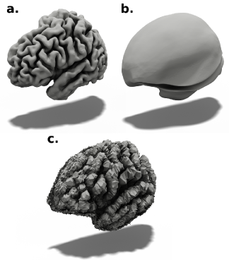
Figure 1: Generating regular meshes of the left hemisphere of the brain cortical surface. a. CorticalFlow, b. NMF with a global feature descriptor [30], c. UNet without diffeomorphic parametrization or geometric penalization.

The reconstruction of regular surfaces from a deformable model is a subtle trade off between finding the right parameterization or a suitable level of regularization during training. The delicacy of this problem is illustrated in Figure 1. First, one can employ multiple penalty functions as Chamfer normal, normal consistency, Laplacian loss, or edge length loss [75, 77]. It is worth mentioning that without such penalizations, a deformable model will learn non-smooth deformations, which leads to irregular meshes (as shown in Figure 1.c). However, those penalizations simply encourage the reconstructed surface to be regular. The second approach consists of parameterizing the set of learned deformations; this approach is favored in our paper since it allows stronger theoretical guarantees and is not subject to hyper-parameter tuning. A natural framework to generate invertible deformations is to consider a flow ODE [20, 73]. This framework has been successfully applied in pattern recognition and image registration [19, 7, 2, 3]. The main idea is to consider the mapping as the solution at time $\tau$ of an initial value problem (IVP) of the form,

$$\frac{\text{d}\Phi(s;\mathbf{x})}{\text{d}s}=v\left(\Phi(s;\mathbf{x}),s\right),\text{ with }\Phi(0;\mathbf{x})=\mathbf{x},$$ (1)

under a regularity hypothesis on $v$ and upon boundedness of its support, and using the Picard-Lidelöf theorem, one can show that a unique solution of this problem exists for $\tau\in\bar{\mathbb{R}}$. In addition, the mapping $\mathbf{x}\mapsto\Phi(s;\mathbf{x})$ defines a family of diffeomorphisms [6, 1] for all time $s\in[0,\tau]$ whose inverse can be computed through a backward integration.

When the vector field $v$ is constant over time i.e. $v:\mathbb{R}^{3}\rightarrow\mathbb{R}^{3}$, Equation (1) describes the Stationary Velocity Field (SVF) framework [1, 3]. If $v$ is a time-varying vector field, the framework described in (1) becomes the LDDMM model [5, 74, 8, 68].

This generic framework has been successfully applied within deep learning methods for diffeomorphic image registration [15, 50], point-cloud completion [52], single view reconstruction [30] and to parameterize set of deformations [37].

The SVF formulation has been particularly fecund in medical deep-learning registration [15, 41, 50, 80], where the resolution of Equation (1), is performed using the scaling and squaring method [2, 3] to predict the displacement of each voxel-center and to compute the registered image. However, this technique is not suitable for points that lie on non-regular coordinates. Naively, one can compute these mappings on a dense grid and then interpolate the deformation at non-regular coordinates. This simple approach is subject to two main limitations. Firstly, Equation (1) has to be solved in our context for millions of grid points where only a few hundred thousand vertices are displaced. Secondly, one cannot guarantee the invertibility of such a mapping with linear interpolation and one cannot compose provably several of those approximated mappings.

In [52, 30], the problem is solved using a black-box neural ODE [9] and by learning a neural vector field $v$. Despite allowing learning a time-dependent vector field, this approach has shown its limitations in our targeted application. Cortical surfaces are unique to each individual; indeed, the cortical folding patterns are similar to a fingerprint [45] and constitute a distinctive biometric for each individual. Moreover, we observe that the classical approach, which consists of conditioning the neural ODE on a global feature descriptor of the input image, fails to provide satisfactory results for cortical surface reconstruction (see Figure 1.b. and the supplementary material). Instead, one has to equip each moving vertex with a local feature descriptor of the input image, limiting the number of vertices of the resulting mesh.

Our work lies at the intersection of these methods. We propose to extend the SVF framework for points lying in real-coordinates, with particular care given to the numerical affordability of the ODE solver. We define a multi-scale approach, so that the final deformation is the result of the composition of three successive deformations that allow to approach more complex mappings and alleviate the limitations of the one vector field SVF framework [44, 23]. This framework is memory efficient, theoretically tractable, and can seamlessly handle large template meshes ($\approx 450\texttt{k}$ vertices).

3 Method

CorticalFlow (CF) is a multi-level deep learning architecture composed of several Diffeomorphic Mesh Deformation (DMD) modules. It takes as input a 3-dimensional Magnetic Resonance Image (MRI) of a patient brain denoted $\mathbf{I}$ (tensor of dimensions $H\times W\times D$) and a template $\mathcal{T}_{i}$ (where $i$ represents the degree of refinement of the template). CorticalFlow outputs the surface representation of an anatomical substructure by composing stackable diffeomorphic deformations generated by DMD modules. CorticalFlow with $k$ deformations ($\text{CF}^{k}$) can be written using the following recurrence,

$$\text{CF}^{1}_{\theta_{1}}(\mathbf{I},\mathcal{T}_{1}) =\text{DMD}(\text{UNet}^{1}_{\theta_{1}}(\mathbf{I}),\mathcal{T}_{1}))$$

$$\text{CF}^{i+1}_{\theta_{i+1}}(\mathbf{I},\mathcal{T}_{i+1}) =\text{DMD}(\text{UNet}^{i+1}_{\theta_{i+1}}(\mathbf{U}_{1}^{\frown}\cdots\mathbf{U}_{i}^{\frown}\mathbf{I}),\text{CF}_{i}(\mathbf{I},\mathcal{T}_{i+1}))\quad\text{for }i\geq 1,$$ (2)

with $\mathbf{A}^{\frown}\mathbf{B}$ the channel-wise concatenation of the tensors $\mathbf{A}$ and $\mathbf{B}$ and where $\mathbf{U}_{k}$ denotes the output of the $k$-th $\text{UNet}^{k}_{\theta_{k}}$ parameterized by $\theta_{k}$.

In our paper we describe $\text{CF}^{3}$, a version of CorticalFlow with three stages where each stage is learned successively. CorticalFlow is trained in a supervised fashion, given a dataset $\mathcal{D}$ composed of pairs of MR-image $\mathbf{I}$ and triangle mesh $S$ representing a cortical structure and for $i\in\{1,2,3\}$ we optimize the following objective,

$$\operatorname*{arg\,min}_{\theta_{i}}\sum_{(\textbf{I},\textbf{S})\in\mathcal{D}}\mathcal{L}\big{(}\text{CF}^{i}_{\theta_{i}}(\mathbf{I},\mathcal{T}_{i}),S).$$ (3)

As training loss $\mathcal{L}(\cdot,\cdot)$, we minimize the mesh edge loss and Chamfer distance computed on point clouds of 150k points sampled from the predicted and ground-truth surfaces using random uniform sampling. The implementation of these losses and sampling algorithm are provided in the PyTorch3D library [60].

3.1 DMD Diffeomorphic Mesh Deformation module

The introduction of a Diffeomorphic Mesh Deformation module (DMD) is driven by the following classification of surfaces in $3$ dimensions:

Theorem 3.1.

Suppose that $B$ is a smooth closed manifold of dimension $2$ embedded in $\mathbb{R}^{3}$. Suppose that $\Phi:[0,\tau]\times\mathbb{R}^{3}\rightarrow\mathbb{R}^{3}$ is a family of homeomorphisms (continuous map such that for each $t$, the mapping $x\mapsto\Phi(t,x)$ is bijective with continuous inverse) , with $\Phi(0;\mathbf{x})=\mathbf{x}$. Then, for each $t$, the homotopy classes of $B$ and $\Phi_{\sharp B}(t)=\left\{\Phi(t,y),y\in B\right\}$ are the same.

This theorem means that if $B$ is a sphere, the surface $\Phi_{\sharp B}(t)$ is of genus $0$ with no self-intersection.

Existence and uniqueness of a solution to the continuous problem

The DMD generation of diffeomorphic mappping relies on the resolution of a continuous flow ODE. For that purpose, let $v:\mathbf{x}\in\Omega\mapsto v(\mathbf{x})\in\mathbb{R}^{3}$ be a constant over time vector field supported on the MRI space $\Omega$ and obtained by tri-linear interpolation of a feature map $\mathbf{U}\in\mathbb{R}^{H\times W\times D\times 3}$. Suppose that $v=0$ on $\partial\Omega$. The image origin is denoted by $O=(o_{1},o_{2},o_{3})$ and denote by $d_{i}$ the interpolation spacing in the $i$-th direction such that $\Omega=[o_{1},o_{1}+d_{1}(H-1)]\times[o_{2},o_{2}+d_{2}(W-1)]\times[o_{3},o_{3}+d_{3}(D-1)]$.

Theorem 3.2.

Existence and uniqueness of the solution. Define $\Phi$ through the autonomous ODE,

$$\frac{\text{d}\Phi(s;\mathbf{x})}{\text{d}s}=v\left(\Phi(s;\mathbf{x})\right),\text{ with }\Phi(0;\mathbf{x})=\mathbf{x}.$$ (4)

Then $\Phi$ is uniquely defined on $\mathbb{R}\times\Omega$, is Lipschitz and for each $t$, the mapping $x\mapsto\Phi(t,x)$ is bijective with Lipschitz inverse. The proof of this result can be found in the supplementary material.

Being Lipschitz is more difficult to achieve than being merely continuous. Less formally, Theorem 3.2 ensures that if $B$ is smooth, then for all $t$, the surface $\Phi_{\sharp B}(t)$ may, in the worst case, have kinks. If $\Phi$ is only continuous and not Lipschitz, then the surface $\Phi_{\sharp B}(t)$ might have cusps that are more irregular than kinks. Note as well that the choice of the interpolation technique used to generate $v$ is pivotal since it drives the regularity of the right-hand side of Equation (6). Indeed, $v$ Lipschitz’s constant boundedness allows the definition of a solution to the continuous problem. More importantly, and as described in the next section, it rules the step-size to use for obtaining a stable numeric method.

Numerical resolution of ODE

The DMD module solves for each vertices’ position a flow ODE defined in Equation (6), defined by $\Psi$ the numeric approximation of $\Phi$ by an explicit forward method, the invertibility of this discretisation is given by the following theorem

Theorem 3.3.

Let $v$ be $L$-Lipschitz. Define $\Psi$ as the Forward Euler approximation,

$$\Psi(h,x)=x+hv(x).$$ (5)

$\Psi$ is a Lipschitz homeomorphism for each $h<L^{-1}$.

As a result, in combination with Theorem 3.2, the surface $\Psi_{\sharp B}(h)$ is smooth as long as $hL<1$. We note that the stability condition $hL<1$ is commonly used in Computational Fluid Dynamics [40]. Less formally, this estimate tells us that the less regular (high gradient) $v$ is, the smaller the integration step should be chosen.

Proof.

Let $h<L^{-1}$ and denote $f:x\mapsto x+hv(x)$. Then $f$ is a Lipschitz mapping and it is sufficient to prove the bijectivity of $f$. The injectivity stems from, for all $x\neq y$,

$$\|f(x)-f(y)\|\geq\|x-y\|-h\|v(x)-v(y)\|\geq\|x-y\|(1-hL)>0.$$

The surjectivity comes from the fact that for each $y$, the mapping $g:x\mapsto y-hv(x)$ is $hL$-Lipschitz with $hL<1$, hence is a contraction. By a fixed point theorem, $g$ admits a unique $x^{\star}$ solution to $g(x^{\star})=x^{\star}$, or equivalently $y=f(x^{\star})$. Hence, $f$ is surjective. ∎

Algorithm 1 DMD module pseudo-code

Input: $\mathbf{U}\in\mathbb{R}^{H\times W\times D\times 3}$ $\triangleright$ Discrete flow

Input: $\mathcal{T}$ with vertices $(V_{i})_{i\in 1..m}$ $\triangleright$ Triangle mesh

Input: $n\in\mathbb{N}^{*}$ $\triangleright$ Number of integration steps

Output: Updated $(V_{i})_{i\in 1..m}$

$h\leftarrow\frac{1}{n}$

$h<\frac{1}{L}$

for $i\in\llbracket 1,m\rrbracket$ do

     for $j\in\llbracket 1,n\rrbracket$ do

         $V_{i}\leftarrow\Psi(h,V_{i})$

     end for

end for

Theorem 3.3 ensures that $\Psi_{\sharp B}(h)$ is a non-intersecting manifold. Unfortunately, there exists another layer of numerical approximation that prevents $\Psi_{\sharp B}(h)$ to have the desired topological properties. Indeed, suppose that $B$ is a sphere, one never computes $\Psi_{\sharp B}(h)$, but triangulates a sphere with vertices $V_{i}$, and evaluates the image of the vertices using Algorithm 1. A new mesh is formed by using the image of the vertices and the original connectivity. Since the perturbed edges of the mesh are not the images of the original edges by the Forward Euler scheme, the resulting mesh may self-intersect (we refer interested readers to Section 2.3 of our supplementary material). Notwithstanding this limitation, we use the rule of thumb $hL\leq 1$, and check that for all considered examples, and we have $hL\leq 1$.

3.2 Network architecture

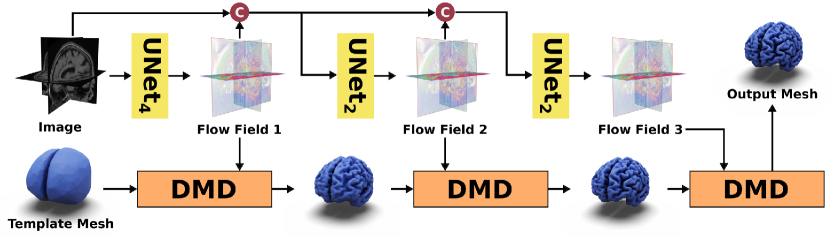
Figure 2: CorticalFlow architecture for the cortical surface reconstruction problem. Following the notations of Equation (3), $\text{UNet}^{1}_{\theta_{1}}$ implements a $\textbf{UNet}_{\textbf{4}}$ layer and $\text{UNet}^{2,3}_{\theta_{2,3}}$ implements a $\textbf{UNet}_{\textbf{2}}$ layer. The architecture of $\textbf{UNet}_{\textbf{4}}$ and $\textbf{UNet}_{\textbf{2}}$ are described in the supplementary materials.

As shown in Figure 2, CorticalFlow consists of a chain of three deformations. Note that more deformation modules could be used, but we focus on three modules to have a fair comparison with existing techniques. The first deformation module receives as input a volumetric image and outputs a flow vector field with the same dimensions using UNet-3D [63]. This discrete flow vector field is integrated by the DMD module to compute smooth deformations as explained in Section 3.1. The subsequent UNet-3D receives as input the image and the flow vector fields predicted by the previous deformation modules. The set of resulting mappings are composed to produce the final mesh.

For training CorticalFlow, we adopted a sequential approach where we train one deformation module at a time while freezing the weights of the others. We train the first deformation with a low-resolution template ($\mathcal{T}_{1}$) of $30\texttt{k}$ vertices and a UNet-3D architecture with four down/up-sampling levels. To train the second and third deformations, we increase the resolution of the template mesh to $135\texttt{k}$ and $435\texttt{k}$ vertices, for $\mathcal{T}_{2}$ and $\mathcal{T}_{3}$ respectively, and reduce the UNet-3D down/up-sampling levels to two. These networks are respectively labeled as $\textbf{UNet}_{\textbf{4}}$ and $\textbf{UNet}_{\textbf{2}}$ in Figure 2 while their layer details are described in our supplementary material. The choice of the architecture depth is motivated by the numerical conditions on the integration step-size derived in Section 3.1.

To verify the conditions of Theorem 3.3, it is essential to mention the use of template meshes with different resolutions and different UNet architectures. Indeed, the first block has to provide a large deformation resulting in a high $\|v\|$. To keep the Lipschitz constant $L$ small, one observes that the use of a low-resolution template with $30\texttt{k}$ vertices along with a deeper convolutional architecture forces the UNet to recover only coarse details and thus produces a flow vector field with a small $\nabla v$. During the second and third deformation, more details and higher resolution folds can be learned, with templates composed of $135\texttt{k}$ and $435\texttt{k}$ vertices, respectively (see the ablation study presented in Section 1.1 of our supplementary material). We empirically verify that this hierarchy of deformations was beneficial for producing a flow vector field $v$ with a small Lipschitz constant. This multi-step approach allows attaining up to $14.5$ times less self-intersection in comparison with Neural Mesh Flow (see Table 1).

To generate the template mesh, we take the convex hull of all surfaces contained in the training dataset and remesh them uniformly using JIGSAW [21]. To achieve a different order of refinement, we use the midpoint subdivision algorithm implemented in MeshLab [12]. Model hyper-parameters and further implementation details are provided in the supplementary material.

4 Experiments

We benchmark CorticalFlow and other existing deep learning techniques on the cortical surface reconstruction problem. The goal is to estimate geometrically accurate and topologically correct triangular meshes for the inner and outer cortical surfaces from a given MRI. Like previous works [14, 16, 34, 38, 31, 65], these surfaces are further divided into the left and right brain hemispheres. See below a summary of the dataset, evaluated methods, and metrics used in our benchmark, in addition to the detailed discussion of the results summarized in Table 1.

Left Outer Surface

Right Outer Surface

CH($mm$) $\downarrow$

HD($mm$) $\downarrow$

CHN $\uparrow$

% SIF $\downarrow$

DSC $\uparrow$

VS $\uparrow$

CH($mm$) $\downarrow$

HD($mm$) $\downarrow$

CHN $\uparrow$

% SIF $\downarrow$

DSC $\uparrow$

VS $\uparrow$

CorticalFlow 1.148 sec / 3.071 GB

$0.681$ $(\pm 0.098)$

$0.802$ $(\pm 0.049)$

$0.932$ $(\pm 0.006)$

$0.686$ $(\pm 0.469)$

$0.977$ $(\pm 0.003)$

$0.993$ $(\pm 0.006)$

$0.693$ $(\pm 0.091)$

$0.815$ $(\pm 0.046)$

$0.929$ $(\pm 0.006)$

$1.239$ $(\pm 0.629)$

$0.976$ $(\pm 0.003)$

$0.994$ $(\pm 0.005)$

DeepCSR 577.492 sec / 11.099 GB

$0.925$ $(\pm 0.265)$

$0.898$ $(\pm 0.135)$

$0.933$ $(\pm 0.011)$

$0.000$ $(\pm 0.000)$

$0.981$ $(\pm 0.003)$

$0.993$ $(\pm 0.005)$

$0.912$ $(\pm 0.208)$

$0.895$ $(\pm 0.125)$

$0.933$ $(\pm 0.010)$

$0.000$ $(\pm 0.000)$

$0.981$ $(\pm 0.003)$

$0.993$ $(\pm 0.005)$

NMF 42.808 sec / 14.431 GB

$1.557$ $(\pm 0.200)$

$1.485$ $(\pm 0.116)$

$0.885$ $(\pm 0.008)$

$0.818$ $(\pm 0.245)$

$0.953$ $(\pm 0.005)$

$0.987$ $(\pm 0.008)$

$1.772$ $(\pm 0.177)$

$1.588$ $(\pm 0.101)$

$0.871$ $(\pm 0.008)$

$1.340$ $(\pm 0.292)$

$0.946$ $(\pm 0.005)$

$0.983$ $(\pm 0.009)$

QuickNAT 13.003 sec / 9.627 GB

$3.732$ $(\pm 1.971)$

$2.582$ $(\pm 1.011)$

$0.874$ $(\pm 0.024)$

$0.000$ $(\pm 0.000)$

$0.956$ $(\pm 0.006)$

$0.975$ $(\pm 0.011)$

$4.282$ $(\pm 2.293)$

$2.800$ $(\pm 1.085)$

$0.870$ $(\pm 0.024)$

$0.000$ $(\pm 0.000)$

$0.954$ $(\pm 0.006)$

$0.971$ $(\pm 0.011)$

Voxel2Mesh 20.840 sec / 23.400 GB

$7.188$ $(\pm 0.669)$

$3.893$ $(\pm 0.218)$

$0.721$ $(\pm 0.016)$

$0.857$ $(\pm 0.260)$

$0.896$ $(\pm 0.008)$

$0.976$ $(\pm 0.011)$

$7.461$ $(\pm 0.711)$

$3.955$ $(\pm 0.227)$

$0.717$ $(\pm 0.017)$

$0.833$ $(\pm 0.260)$

$0.888$ $(\pm 0.008)$

$0.967$ $(\pm 0.010)$

Left Inner Surface

Right Inner Surface

CH($mm$) $\downarrow$

HD($mm$) $\downarrow$

CHN $\uparrow$

% SIF $\downarrow$

DSC $\uparrow$

VS $\uparrow$

CH($mm$) $\downarrow$

HD($mm$) $\downarrow$

CHN $\uparrow$

% SIF $\downarrow$

DSC $\uparrow$

VS $\uparrow$

CorticalFlow 1.148 sec / 3.071 GB

$0.608$ $(\pm 0.098)$

$0.785$ $(\pm 0.060)$

$0.941$ $(\pm 0.007)$

$0.033$ $(\pm 0.030)$

$0.962$ $(\pm 0.005)$

$0.987$ $(\pm 0.010)$

$0.599$ $(\pm 0.093)$

$0.783$ $(\pm 0.059)$

$0.942$ $(\pm 0.007)$

$0.030$ $(\pm 0.029)$

$0.962$ $(\pm 0.005)$

$0.987$ $(\pm 0.010)$

DeepCSR 577.492 sec / 11.099 GB

$0.653$ $(\pm 0.138)$

$0.767$ $(\pm 0.063)$

$0.956$ $(\pm 0.006)$

$0.000$ $(\pm 0.000)$

$0.963$ $(\pm 0.006)$

$0.985$ $(\pm 0.012)$

$0.634$ $(\pm 0.139)$

$0.760$ $(\pm 0.057)$

$0.956$ $(\pm 0.006)$

$0.000$ $(\pm 0.000)$

$0.964$ $(\pm 0.006)$

$0.986$ $(\pm 0.011)$

NMF 42.808 sec / 14.431 GB

$1.404$ $(\pm 0.185)$

$1.447$ $(\pm 0.140)$

$0.884$ $(\pm 0.011)$

$0.355$ $(\pm 0.168)$

$0.928$ $(\pm 0.006)$

$0.984$ $(\pm 0.012)$

$1.434$ $(\pm 0.184)$

$1.463$ $(\pm 0.135)$

$0.883$ $(\pm 0.010)$

$0.436$ $(\pm 0.188)$

$0.927$ $(\pm 0.006)$

$0.984$ $(\pm 0.012)$

QuickNAT 13.003 sec / 9.627 GB

$2.370$ $(\pm 1.893)$

$1.836$ $(\pm 0.734)$

$0.906$ $(\pm 0.023)$

$0.000$ $(\pm 0.000)$

$0.905$ $(\pm 0.027)$

$0.924$ $(\pm 0.031)$

$2.295$ $(\pm 1.963)$

$1.788$ $(\pm 0.725)$

$0.908$ $(\pm 0.023)$

$0.000$ $(\pm 0.000)$

$0.906$ $(\pm 0.027)$

$0.931$ $(\pm 0.031)$

Voxel2Mesh 20.840 sec / 23.400 GB

$5.968$ $(\pm 0.657)$

$3.461$ $(\pm 0.247)$

$0.703$ $(\pm 0.017)$

$0.621$ $(\pm 0.220)$

$0.850$ $(\pm 0.009)$

$0.982$ $(\pm 0.014)$

$6.172$ $(\pm 0.719)$

$3.549$ $(\pm 0.272)$

$0.707$ $(\pm 0.017)$

$0.761$ $(\pm 0.271)$

$0.842$ $(\pm 0.010)$

$0.971$ $(\pm 0.018)$

Table 1: Cortical Surface Reconstruction Benchmark. Consider the evaluation metrics: chamfer distance (CH), Hausdorff distance (HD), chamfer normals (CHN), percentage of self-intersecting faces (%SIF), Dice Score (DSC), and Volume Similarity (VS). $\downarrow$ indicates smaller metric value is better, while $\uparrow$ indicates greater metric value is better. We also report the inference runtime and GPU memory footprint required by the compared algorithms.

Dataset.

We used the same MRIs, pseudo-ground-truth surfaces, and data splits as [65]. This dataset consists of 3,876 MRI images extracted from the Alzheimer’s Disease Neuroimaging Initiative (ADNI) [36] and their respective pseudo-ground-truth surfaces generated with the FreeSurfer V6.0 cross-sectional pipeline [25]. We train all methods on the training set ($\approx 60$%) until their losses plateau on the validation set ($\approx 10$%) and report their performance on the test set ($\approx 30$%). We refer the reader to [65] and our supplementary material for full details on the dataset.

Evaluated Methods.

We compare CorticalFlow to the following methods: DeepCSR [65], Voxel2Mesh [77], NMF [30], and QuickNAT [64]. As discussed in Section 2, DeepCSR is the state-of-the-art geometric deep learning model for cortical surface reconstruction, while Voxel2Mesh is a deformation-based model proposed to retrieve generic anatomical surfaces from volumetric medical images like MRIs and CT scans. Differently, NMF is a deformation-based model for single-view object reconstruction from 2D images. To adapt this model to our task whose input is a 3D MRI, we evaluate different 3D convolutional network backbones based on UNet [63], ResNet [33], and Hypercolumn [65]. The Hypercolumn backbone provides the best results thanks to its vertex-dependent features. As such, this is used as the NMF backbone in our benchmark. At the same time, the results for the other backbones are presented in our supplementary material. We also evaluate a baseline composed of a state-of-the-art brain segmentation model QuickNAT [64] followed with the marching cubes to evaluate the surface. All of these methods were trained and evaluated using a NVIDIA P100 GPU and Intel Xeon (E5-2690) CPU, except Voxel2Mesh which required a NVIDIA RTX 3090 GPU due to its GPU memory requirements.

Evaluation Metrics.

We compare these methods for their geometric accuracy and surface regularity, as well as their time and space complexity. As a measure of geometric accuracy, we report the standard Chamfer distance (CH), Hausdorff distance (HD), and Chamfer normals (CHN). We compute these distances for point clouds of $200\texttt{k}$ points uniformly sampled from the predicted and target surfaces. As a measure of regularity, we compute the percentage of self-intersecting faces (%SIF) using PyMeshLab [51]. We also report volumetric overlap metrics [71] including Dice Score (DSC) and Volume Similarity (VS) computed on the high-resolution rasterization ($4\times$the input MRI resolution) of the generated and ground-truth surfaces.

For the time and space complexity of the evaluated methods, we report their average inference time (in seconds) and inference GPU memory footprint (in GB) to reconstruct the four cortical surfaces, respectively.

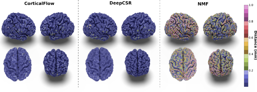
Figure 3: Predicted outer cortical surfaces color-coded with the distance to the pseudo-ground-truth surfaces. Here we present the results for the three best-performing methods in terms of geometric accuracy: CorticalFlow, DeepCSR, and NMF. See our supplementary materials for more examples.

Results & Discussion.

In our experiments, we noticed that CorticalFlow produces more geometrically accurate surfaces than the other methods. On average, it presents better geometric metrics across all the cortical surfaces. In addition, as shown in Figure 3, CorticalFlow errors are smaller ($\leq 0.2mm$) and evenly spread across the surface compared to the other methods. In contrast, NMF and DeepCSR can present substantial errors ($\geq 1mm$). The former has its error spread across the entire surface, while the latter can produce large errors at specific regions.

CorticalFlow is also more robust than the competitors presenting lower error variation across individuals as suggested by the smaller standard deviation of the geometric metrics computed. Interestingly, CorticalFlow is also more robust to MRI artifacts even when the pseudo-ground-truth surface has poor quality. For instance, in Figure 4, CorticalFlow predictions are still plausible for a blurry input MRI while FreeSurfer fails significantly to generate appropriate surfaces for the same input. These examples support our claim that a regular parametrization allows us to reduce non-plausible and non-diffeomorphic predictions that our model cannot learn by construction.

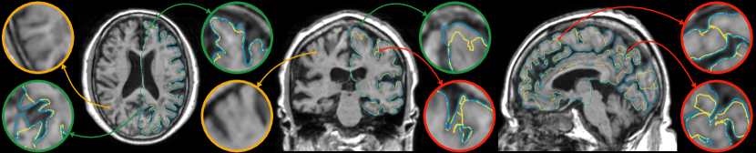
Figure 4: Slices of a blurry MRI and the outer surface delineation generated by FreeSurfer V6 (yellow contour) and CorticalFlow (blue contour). Orange circles highlight blurry MRI regions, green circles highlight FreeSurfer’s underestimated areas, while red circles highlight non-plausible predictions avoided by CorticalFlow thanks to the diffeomorphism of its predicted deformations.

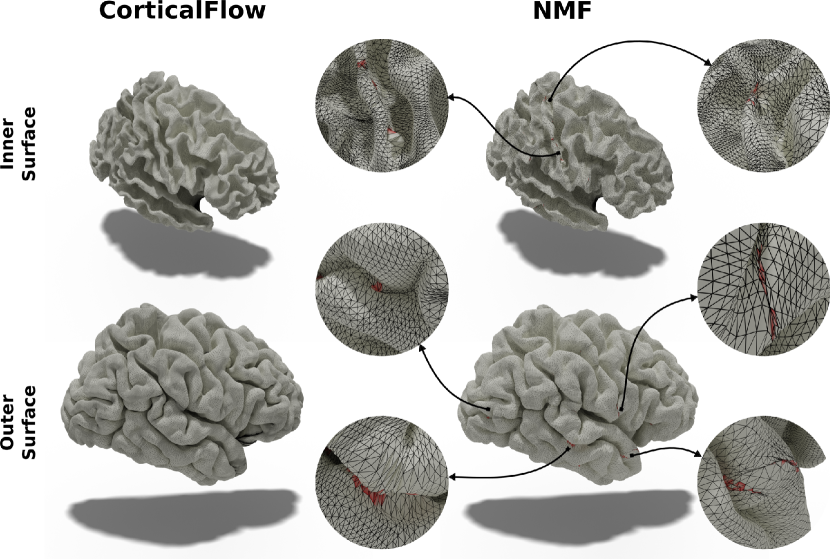
(a)

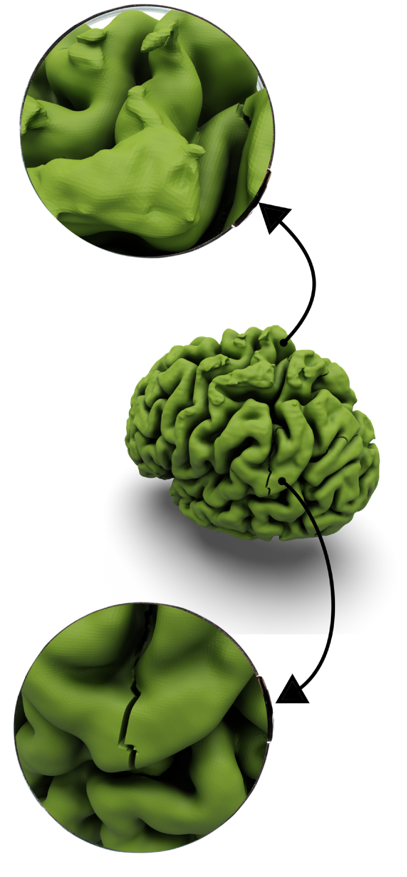
(b)

Figure 5: 5(a): Predicted cortical surfaces by CorticalFlow and NMF with self-intersecting faces highlighted in red. 5(b): Significant mistakes generated by the topology correction algorithm used in the DeepCSR method.

CorticalFlow also generates triangular meshes with better properties than the evaluated methods. Compared to the deformation-based methods NMF and Voxel2Mesh, CorticalFlow predicted meshes are genus-zero surfaces and present a lower percentage of self-intersecting faces (mainly for the inner cortical surfaces). Figure 5(a) presents examples of self-intersecting faces produced by CorticalFlow, which are contrasted with the NMF predicted mesh for the same input MRI. The implicit-surface-based DeepCSR method does not produce a single self-intersecting face since it employs computationally expensive post-processing routines like topology correction [4] and iso-surface extraction. However, these post-processing routines do not take into account the input MRI which can generate non-plausible corrections on the output mesh as previously observed in Segonne et al. [67] and exemplified in Figure 5(b). Similarly, the voxel-wise segmentation baseline (i.e., QuickNAT) is free of self-intersecting faces, but it does not produce genus-zero surfaces. Indeed, QuickNAT’s predicted surfaces are composed of multiple connected components presenting many handles and holes which is not acceptable for the purpose of cortical surface reconstruction. Some examples of QuickNAT reconstructed cortical surfaces are presented in our supplementary material. Therefore, we argue that CorticalFlow is the method of choice to reconstruct regular surfaces from volumetric images.

Due to its elemental construction (three UNet-3D backbones and an interpolation module for the integration), CorticalFlow remains highly efficient. It has a minimal GPU memory footprint and faster inference runtime while handling larger surfaces with more vertices both during training and inference. This feature allows its deployment on low-end computers and embedded devices which is pivotal in many scenarios across public health and for commercialization of affordable AI healthcare solutions [13, 58].

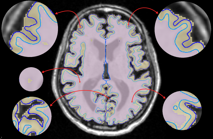
(a)

(b)

Figure 6: 6(a): QuickNAT segmentation (inner surface volume in pink and outer surface volume in yellow) and CorticalFlow generated surfaces (inner surface in light blue and outer surface in dark blue). Note that the highlighted artifacts in QuickNAT segmentation can be easily surpassed by CorticalFlow thanks to its continuous representation of the region of interest. 6(b): Outer cortical surface color-coded with the curvature of its cortical foldings. Our method allows us to map back this measure and any other biomarker to the input template using the composition of the inverse deformations $\Phi^{-1}$.

Finally, as a by-product of CorticalFlow’s deformable and diffeomorphic nature, one can seamlessly obtain a sub-voxel resolution segmentation by applying a voxelization engine. This can capture variations below the image resolution while traditional segmentation methods [64] are restrained from working at the image resolution (see Figure 6(a)). Additionally, an essential component of computational neuro-anatomy consists of computing local shape descriptors for different individuals and transferring them to the same reference space using conformal mappings [29, 70]. For the proposed model, one can efficiently compute the inverse transformation $\Phi^{-1}$ as shown in Figure 6(b) for the surface curvature descriptor.

5 Conclusion

This paper introduces CorticalFlow - a geometric deep learning model for efficiently reconstructing high-resolution, accurate, and regular triangular meshes from volumetric images. We develop a lightweight neural network to predict a dense 3D flow vector field from a volumetric image. Then, we describe a new Diffeomorphic Mesh Deformation (DMD) module, which is parameterized by a set of diffeomorphic mappings. This includes the derivation of numerical conditions for recasting the continuous flow ODE problem into an efficient discrete solver. Finally, we extensively verify that the proposed model achieves state-of-the-art performance in the challenging brain cortical surface reconstruction problem. This benchmark reveals that CorticalFlow is more accurate and, by construction, more robust to image artifacts providing anatomically plausible surfaces. Thanks also to its low space and time complexity, the proposed method can facilitate large-scale medical studies and support new healthcare applications.

6 Compliance with Ethical Standards

This research was approved by CSIRO ethics 2020 068 LR.

7 Acknowledgements

This work was funded in part through an Australian Department of Industry, Energy and Resources CRC-P project between CSIRO, Maxwell Plus and I-Med Radiology Network.

 
Supplementary Material

 

Implementation details

 

Ablation study for Cortical Flow: number of deformation blocks

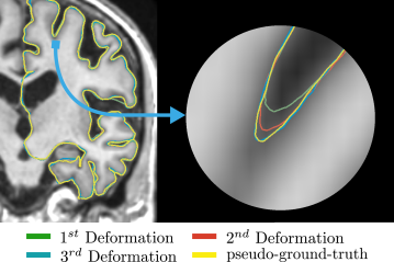
Figure 7: Example of MRI slice and outer cortical surface predicted at different deformation blocks of the proposed CorticalFlow. Zoomed in sulci region to visualize the improvements provided by the sequence of deformation predicted by CorticalFlow.

As explained in subsection 3 of our paper, CorticalFlow leverages a chain of 3 deformation blocks to provide a coarse-to-fine approximation of the targeted surface. We evaluate CorticalFlow predictions after each deformation block in our cortical surface reconstruction benchmark to empirically validate this modeling decision. As shown in Table 2, every deformation block added allows a better approximation of the ground-truth surfaces. More specifically, on average across all surfaces, adding a second deformation block reduces the Chamfer distance metric by 36.73%, while adding a third deformation block reduces the same metric by a further 5.06%. Importantly, this error reduction is more evident in the sulci region of the cortical surfaces, as shown by the example depicted in Figure 7.

	Left Outer Surface			Right Outer Surface
Number of Deformation Blocks	CH($mm$) $\downarrow$	HD($mm$) $\downarrow$	CHN $\uparrow$	CH($mm$) $\downarrow$	HD($mm$) $\downarrow$	CHN $\uparrow$
1	$1.176$ $(\pm 0.143)$	$1.223$ $(\pm 0.097)$	$0.903$ $(\pm 0.008)$	$1.300$ $(\pm 0.148)$	$1.328$ $(\pm 0.103)$	$0.898$ $(\pm 0.009)$
2	$0.716$ $(\pm 0.102)$	$0.833$ $(\pm 0.056)$	$0.932$ $(\pm 0.006)$	$0.741$ $(\pm 0.095)$	$0.855$ $(\pm 0.055)$	$0.929$ $(\pm 0.006)$
3	$0.681$ $(\pm 0.098)$	$0.802$ $(\pm 0.049)$	$0.932$ $(\pm 0.006)$	$0.693$ $(\pm 0.091)$	$0.815$ $(\pm 0.046)$	$0.929$ $(\pm 0.006)$
	Left Inner Surface			Right Inner Surface
Number of Deformation Blocks	CH($mm$) $\downarrow$	HD($mm$) $\downarrow$	CHN $\uparrow$	CH($mm$) $\downarrow$	HD($mm$) $\downarrow$	CHN $\uparrow$
1	$0.952$ $(\pm 0.147)$	$1.125$ $(\pm 0.133)$	$0.918$ $(\pm 0.009)$	$0.917$ $(\pm 0.124)$	$1.079$ $(\pm 0.105)$	$0.919$ $(\pm 0.009)$
2	$0.636$ $(\pm 0.101)$	$0.814$ $(\pm 0.067)$	$0.941$ $(\pm 0.007)$	$0.627$ $(\pm 0.097)$	$0.811$ $(\pm 0.066)$	$0.942$ $(\pm 0.007)$
3	$0.608$ $(\pm 0.098)$	$0.785$ $(\pm 0.060)$	$0.941$ $(\pm 0.007)$	$0.599$ $(\pm 0.093)$	$0.783$ $(\pm 0.059)$	$0.942$ $(\pm 0.007)$

Table 2: Evaluation of the proposed CorticalFlow model with different number of deformation blocks in the cortical surface reconstruction benchmark. Consider the evaluation metrics: chamfer distance (CH), Hausdorff distance (HD), and chamfer normals (CHN). $\downarrow$ indicates smaller metric value is better, while $\uparrow$ indicates greater metric value is better.

Cortical Flow Architecture and Training details

As shown in Figure 2 of our paper, CorticalFlow consists of a chain of three deformation blocks. Each of these deformations is implemented by some UNet flow vector field predictor and the Diffeomorphic Mesh Deformation (DMD) module described in subsection 3.1 of our paper. More specifically, the first deformation block uses our $\textbf{UNet}_{\textbf{4}}$ architecture while the remaining ones use our $\textbf{UNet}_{\textbf{2}}$ architecture. Both architectures are described in details in Figure 8. As explained in subsection 3.2, the reason for this architectural change is to promote the learning of a coarse-to-fine sequence of deformation blocks.

For training CorticalFlow, we adopted a sequential approach where we train one deformation block at a time while freezing the weights of the previous UNet(s). All deformation blocks are trained according to equation 2 for 70k iterations with a batch size of three image-surface pairs. As training loss $\mathcal{L}(\cdot,\cdot)$, we minimize the mesh edge loss and Chamfer distance computed on point clouds of 150k points sampled from the predicted and ground-truth surfaces using random uniform sampling. The implementation of these losses and sampling algorithm are provided in the PyTorch3D library [60]. As an optimizer for each deformation, we use Adam [39] with an initial learning rate of $10^{-4}$. Both predicted and ground-truth surfaces are shrunk to lie in the unit ball to normalize the learning loss.

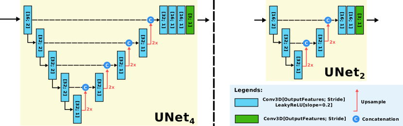
Figure 8: UNet architectures used in CorticalFlow. See Figure 2 of our paper for a global overview of the model.

Backbone selection for Neural Mesh Flow (NMF)

Neural Mesh Flow (NMF) is a deformation-based geometric deep learning model for retrieving regular surfaces for objects depicted in a single 2D image. This model has two main blocks: an image-level feature encoder and a mesh transformer. The former is composed of a ResNet [33] point-cloud predictor and a PointNet [59] network providing an image-level feature vector representation for an input 2D image. The latter receives this image-level feature vector as input and deforms a prescribed template towards the ground-truth surface using Neural Ordinary Differential Equation (NODE) blocks. To adapt this model to cortical surface reconstruction performing only minimal changes, we swap the architecture of the point-cloud predictor from a 2D ResNet to a 3D ResNet. However, as shown in the first row of Figure 9, the resulting model performs very poorly in the cortical surface reconstruction task. More specifically, We found it very hard to predict point clouds to cortical surfaces since these surfaces present many local dissimilarities (e.g., cortical folding patterns) that are hard to capture by funnel-like architectures like ResNet. Trying to overcome this problem, we replaced the ResNet with a 3D UNet [63] with shortcut connections (i.e., our Unet₄ architecture) to exploit high-resolution feature maps within the computation of the image-level feature vector representation. As shown in the second row of Figure 9, the results were still far from satisfactory. As discussed in subsection 2.2 and also observed by Santa Cruz et al. [65], an image-level feature vector does not hold fine-grained information enough to reconstruct cortical surfaces accurately. Therefore, we tried their proposed Hypercolumns architecture which equips each template vertex with a local feature descriptor of the input image resulting in more accurate cortical surface reconstructions as shown in the last row of Figure 9. Therefore, the NMF with Hypercolumns backbone is the NMF model used in our benchmark, whose results are summarized in Table 1 of our paper.

Figure 9: Outer cortical surface reconstruction for four subjects (columns) using the NMF framework with different backbones. The Hypercolumns backbone is significantly better than the others, and thus it is the NMF’s backbone presented in our benchmark.

QuickNAT Baseline

The QuickNAT baseline consists of a voxel-wise segmentation model, iso-surface extraction method, and a mesh post-processing routine. More specifically, we first predict a segmentation of the input MRI into 28 anatomical regions using the QuickNAT [64] state-of-the-art segmentation model for brain segmentation. Second, we build the four cortical volumes by assembling anatomical structures contained in the four surfaces. Third, we run a marching cubes [42] algorithm to retrieve triangle meshes from the obtained binary segmentations. Since the resulting meshes present a lot of unwanted connected components (due to spurious mistakes in the segmentation), we only isolate the largest connected component using the trimesh.graph.connected_component_labels function. Figure 10 presents some meshes generated with this QuickNAT baseline. Our methodology was to get the best geometrical measure stemming from a segmentation-based approach. We verify that the suppression of small connected components improves all the metrics presented in our paper. Note, however, that those meshes cannot be used for the cortical surface reconstruction problem since they comprise hole and handle (not 0-genus). It is also important to notice that numerous errors are imputable to the limited resolution of this approach.

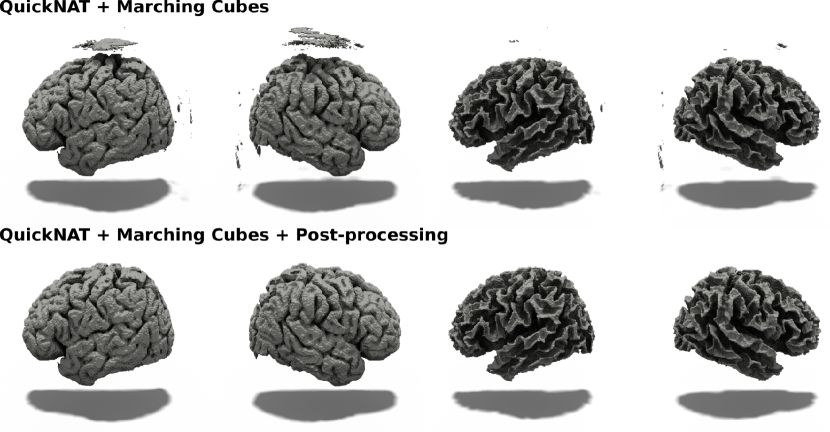
Figure 10: Cortical Surfaces generated with the QuickNAT baseline before and after the post-processing routine.

Dataset Information and Preprocessing

The dataset used in the experiments described in subsection 4 of our paper was introduced in [65]. It consists of MR images extracted from the Alzheimer’s Disease Neuroimaging Initiative (ADNI) [36] and their respective pseudo-ground-truth surfaces generated with the FreeSurfer V6.0 cross-subsectional pipeline [25, 24]. It comprises 3876 MR images from 820 different subjects collected at different time points and their respective cortical surfaces split by brain hemisphere (i.e., left outer surface, left inner surface, right outer surface, and right inner surface). This dataset is split by subjects resulting in 2353 MRI scans from 492 subjects for training ($\approx 60\%$), 375 MRI scans from 82 subjects for validation ($\approx 10\%$), and 1148 MRI scans from 246 subjects for testing ($\approx 30\%$). It is also important to emphasize that these splits do not have MRIs or subjects in common for an unbiased evaluation.

As preprocessing, the original ADNI images are conformed and normalized according to the first steps in the FreeSurfer V6 pipeline. These images are saved at <subject_id>/mri/orig.mgz on the FreeSurfer output directory. Then, they are affine registered to the MNI105 brain template [46] using the NiftyReg toolbox [49]. Their respective pseudo-ground-truth surfaces are also transformed using the computed transformation. Finally, for memory efficiency, these images are split by hemisphere since we learn a model for each surface resulting in 1$mm^{2}$ isotropic T1-weighted images with $96\times 192\times 160$ dimensions. Detailed instructions for downloading and preprocessing this data will be provided along with our source code.

Proof and discussion

 

Proof of Theorem 3.2.

Theorem 3.2.

Existence and uniqueness of the solution. Define $\Phi$ through the autonomous ODE,

$$\frac{\text{d}\Phi(s;\mathbf{x})}{\text{d}s}=v\left(\Phi(s;\mathbf{x})\right),\text{ with }\Phi(0;\mathbf{x})=\mathbf{x}.$$ (6)

Then $\Phi$ is uniquely defined on $\mathbb{R}\times\Omega$, is Lipschitz and for each $t$, the mapping $x\mapsto\Phi(t,x)$ is bijective with Lipschitz inverse.

Proof.

This is a standard result in flow theory; see Theorem 1.2.6 Berger and Gostiaux [6].

1. First, notice that the vector field $v$ is L-Lipschitz with $L>0$ defined as

   $$L=\text{Lip}(v)=\max_{i\in\{1,2,3\}}\frac{\|\nabla_{i}\mathbf{U}\|_{2,\infty}}{d_{i}}$$

   with $\nabla_{d}\mathbf{U}$ the forward first order finite difference operator in the $d$-th direction with zero padding

   $$\nabla_{1}U_{i,j,k}=\begin{cases}\text{if }i\in\llbracket 1,n-1\rrbracket,\quad U_{i+1,j,k}-U_{i,j,k}\\ \text{if }i\in\{0,n\},\quad U_{i,j,k}.\end{cases}$$

2. Then verify that vector field $v$ is bounded by $M$ with $M=\|v\|_{2,\infty}=\max_{i,j,k}\|\mathbf{U}_{ijk}\|_{2}$

With these two constants one can use the result of Berger and Gostiaux [6] (Theorem 1.2.6) to define a unique local solution for $t\in]-b,b[$ with $b<\inf(\frac{\text{diam}(\Omega)}{M},\frac{1}{L})$ where $\text{diam}(\Omega)$ is the diameter of the set $\Omega$.

To extend this result for all $t\in\mathbb{R}$, one has to notice that the solution is defined for every $t$ since the integral solutions are contained in $\Omega$ since $v=0$ on $\partial\Omega$. To construct the inverse, one uses the same proof method but integrates $v$ from $t$ to zero. ∎

Caveat: Discrete approximation of continuous surfaces

Figure 11: Deformation of a template mesh. From left to right: The original triangle mesh, a prescribed vector-field $v$, deformed triangulation where the map $\Psi$ applied on the mesh’s vertices creating a self-intersection, and continuous deformation of triangle mesh’ surface by $\Psi$.

As explained at the end of Section 3.1, $\Psi$ being a homeomorphism does not guarantee that the discrete problem we are solving is immune to self-intersection, and such a pathological case is described in Figure 11. Note, however, that one could get rid of the self-intersection up to sufficient remeshing of the self-intersecting faces. This discretization issue has to be kept in mind when using a deformable model that acts on the vertices of a triangle mesh.

Further comparison with pre-existing methods

 

Comparison with DeepCSR and NMF

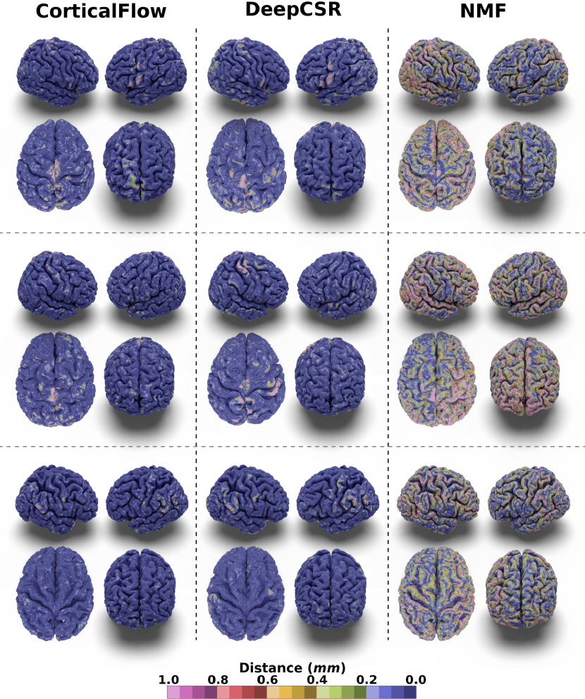
Figure 12: More examples of predicted outer cortical surfaces color-coded with the distance to the pseudo-ground-truth surfaces as shown in Figure 3 of our paper. Here, each row presents the results for a different input MRI. All the presented anatomies are included between the $40$th and $60$th percentile for the Chamfer distance.

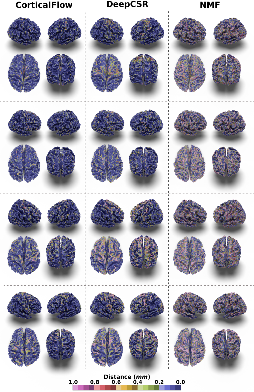
Figure 13: More examples of predicted inner cortical surfaces color-coded with the distance to the pseudo-ground-truth surfaces as shown in Figure 3 of our paper. Here, each row presents the results for a different input MRI. All the presented anatomies are included between the $40$th and $60$th percentile for the Chamfer distance.

References

- Arsigny [2004] Vincent Arsigny. Processing data in lie groups: an algebraic approach. application to non-linear registration and diffusion tensor mri. PhD thesis, Citeseer, 2004.
- Arsigny et al. [2005] Vincent Arsigny, Xavier Pennec, and Nicholas Ayache. Polyrigid and polyaffine transformations: a novel geometrical tool to deal with non-rigid deformations–application to the registration of histological slices. Medical image analysis, 9(6):507–523, 2005.
- Ashburner [2007] John Ashburner. A fast diffeomorphic image registration algorithm. Neuroimage, 38(1):95–113, 2007.
- Bazin and Pham [2007] Pierre-Louis Bazin and Dzung L Pham. Topology correction of segmented medical images using a fast marching algorithm. Computer methods and programs in biomedicine, 88(2):182–190, 2007.
- Beg et al. [2005] M Faisal Beg, Michael I Miller, Alain Trouvé, and Laurent Younes. Computing large deformation metric mappings via geodesic flows of diffeomorphisms. International journal of computer vision, 61(2):139–157, 2005.
- Berger and Gostiaux [2012] Marcel Berger and Bernard Gostiaux. Differential Geometry: Manifolds, Curves, and Surfaces: Manifolds, Curves, and Surfaces, volume 115. Springer Science & Business Media, 2012.
- Camion and Younes [2001] Vincent Camion and Laurent Younes. Geodesic interpolating splines. In International workshop on energy minimization methods in computer vision and pattern recognition, pages 513–527. Springer, 2001.
- Charon [2013] Nicolas Charon. Analysis of geometric and functional shapes with extensions of currents: applications to registration and atlas estimation. PhD thesis, École normale supérieure de Cachan-ENS Cachan, 2013.
- Chen et al. [2018] Ricky T. Q. Chen, Yulia Rubanova, Jesse Bettencourt, and David Duvenaud. Neural ordinary differential equations. Advances in Neural Information Processing Systems, 2018.
- Chen et al. [2020] Zhiqin Chen, Andrea Tagliasacchi, and Hao Zhang. Bsp-net: Generating compact meshes via binary space partitioning. In Proceedings of the IEEE/CVF Conference on Computer Vision and Pattern Recognition, pages 45–54, 2020.
- Choy et al. [2016] Christopher B Choy, Danfei Xu, JunYoung Gwak, Kevin Chen, and Silvio Savarese. 3d-r2n2: A unified approach for single and multi-view 3d object reconstruction. In European conference on computer vision, pages 628–644. Springer, 2016.
- Cignoni et al. [2008] Paolo Cignoni, Marco Callieri, Massimiliano Corsini, Matteo Dellepiane, Fabio Ganovelli, and Guido Ranzuglia. MeshLab: an Open-Source Mesh Processing Tool. In Vittorio Scarano, Rosario De Chiara, and Ugo Erra, editors, Eurographics Italian Chapter Conference. The Eurographics Association, 2008. ISBN 978-3-905673-68-5. doi: 10.2312/LocalChapterEvents/ItalChap/ItalianChapConf2008/129-136.
- Cooley et al. [2020] Clarissa Z Cooley, Patrick C McDaniel, Jason P Stockmann, Sai Abitha Srinivas, Stephen Cauley, Monika Sliwiak, Charlotte R Sappo, Christopher F Vaughn, Bastien Guerin, Matthew S Rosen, et al. A portable brain mri scanner for underserved settings and point-of-care imaging. arXiv preprint arXiv:2004.13183, 2020.
- Dahnke et al. [2013] Robert Dahnke, Rachel Aine Yotter, and Christian Gaser. Cortical thickness and central surface estimation. NeuroImage, 65:336–348, 2013.
- Dalca et al. [2019] Adrian V Dalca, Guha Balakrishnan, John Guttag, and Mert R Sabuncu. Unsupervised learning of probabilistic diffeomorphic registration for images and surfaces. Medical image analysis, 57:226–236, 2019.
- Dale et al. [1999] Anders M Dale, Bruce Fischl, and Martin I Sereno. Cortical surface-based analysis: I. segmentation and surface reconstruction. NeuroImage, 9(2):179–194, 1999.
- Deng et al. [2020] Boyang Deng, Kyle Genova, Soroosh Yazdani, Sofien Bouaziz, Geoffrey Hinton, and Andrea Tagliasacchi. Cvxnet: Learnable convex decomposition. In Proceedings of the IEEE/CVF Conference on Computer Vision and Pattern Recognition, pages 31–44, 2020.
- Du et al. [2007] An-Tao Du, Norbert Schuff, Joel H Kramer, Howard J Rosen, Maria Luisa Gorno-Tempini, Katherine Rankin, Bruce L Miller, and Michael W Weiner. Different regional patterns of cortical thinning in alzheimer’s disease and frontotemporal dementia. Brain, 130(4):1159–1166, 2007.
- Dupuis et al. [1998] Paul Dupuis, Ulf Grenander, and Michael I Miller. Variational problems on flows of diffeomorphisms for image matching. Quarterly of applied mathematics, pages 587–600, 1998.
- Ebin and Marsden [1970] David G Ebin and Jerrold Marsden. Groups of diffeomorphisms and the motion of an incompressible fluid. Annals of Mathematics, pages 102–163, 1970.
- Engwirda and Ivers [2016] Darren Engwirda and David Ivers. Off-centre steiner points for delaunay-refinement on curved surfaces. Computer-Aided Design, 72:157–171, 2016.
- Fahim et al. [2021] George Fahim, Khalid Amin, and Sameh Zarif. Single-view 3d reconstruction: A survey of deep learning methods. Computers & Graphics, 94:164–190, 2021.
- Feydy [2020] Jean Feydy. Analyse de données géométriques, au delà des convolutions. PhD thesis, Université Paris-Saclay, 2020.
- Fischl et al. [1999] Bruce Fischl, Martin I Sereno, and Anders M Dale. Cortical surface-based analysis: Ii: inflation, flattening, and a surface-based coordinate system. Neuroimage, 9(2):195–207, 1999.
- Fischl et al. [2002] Bruce Fischl, David H Salat, Evelina Busa, Marilyn Albert, Megan Dieterich, Christian Haselgrove, Andre Van Der Kouwe, Ron Killiany, David Kennedy, Shuna Klaveness, et al. Whole brain segmentation: automated labeling of neuroanatomical structures in the human brain. Neuron, 33(3):341–355, 2002.
- Genova et al. [2019] Kyle Genova, Forrester Cole, Daniel Vlasic, Aaron Sarna, William T Freeman, and Thomas Funkhouser. Learning shape templates with structured implicit functions. In Proceedings of the IEEE/CVF International Conference on Computer Vision, pages 7154–7164, 2019.
- Girdhar et al. [2016] Rohit Girdhar, David F Fouhey, Mikel Rodriguez, and Abhinav Gupta. Learning a predictable and generative vector representation for objects. In European Conference on Computer Vision, pages 484–499. Springer, 2016.
- Groueix et al. [2018] Thibault Groueix, Matthew Fisher, Vladimir G Kim, Bryan C Russell, and Mathieu Aubry. A papier-mâché approach to learning 3d surface generation. In Proceedings of the IEEE conference on computer vision and pattern recognition, pages 216–224, 2018.
- Gu et al. [2004] Xianfeng Gu, Yalin Wang, Tony F Chan, Paul M Thompson, and Shing-Tung Yau. Genus zero surface conformal mapping and its application to brain surface mapping. IEEE transactions on medical imaging, 23(8):949–958, 2004.
- Gupta and Chandraker [2020] Kunal Gupta and Manmohan Chandraker. Neural mesh flow: 3d manifold mesh generation via diffeomorphic flows. In Advances in Neural Information Processing Systems, volume 33, pages 1747–1758, 2020.
- Han et al. [2004] Xiao Han, Dzung L Pham, Duygu Tosun, Maryam E Rettmann, Chenyang Xu, and Jerry L Prince. Cruise: cortical reconstruction using implicit surface evolution. NeuroImage, 23(3):997–1012, 2004.
- Hanocka et al. [2020] Rana Hanocka, Gal Metzer, Raja Giryes, and Daniel Cohen-Or. Point2mesh: A self-prior for deformable meshes. ACM Trans. Graph., 39(4), 2020.
- He et al. [2016] Kaiming He, Xiangyu Zhang, Shaoqing Ren, and Jian Sun. Deep residual learning for image recognition. In Proceedings of the IEEE conference on computer vision and pattern recognition, pages 770–778, 2016.
- Henschel et al. [2020] Leonie Henschel, Sailesh Conjeti, Santiago Estrada, Kersten Diers, Bruce Fischl, and Martin Reuter. Fastsurfer-a fast and accurate deep learning based neuroimaging pipeline. NeuroImage, page 117012, 2020.
- Häne et al. [2017] Christian Häne, Shubham Tulsiani, and Jitendra Malik. Hierarchical surface prediction for 3d object reconstruction. In 2017 International Conference on 3D Vision (3DV), pages 412–420, 2017. doi: 10.1109/3DV.2017.00054.
- Jack Jr et al. [2008] Clifford R Jack Jr, Matt A Bernstein, Nick C Fox, Paul Thompson, Gene Alexander, Danielle Harvey, Bret Borowski, Paula J Britson, Jennifer L. Whitwell, Chadwick Ward, et al. The alzheimer’s disease neuroimaging initiative (adni): Mri methods. Journal of Magnetic Resonance Imaging, 27(4):685–691, 2008.
- Jiang et al. [2020] Chiyu Jiang, Jingwei Huang, Andrea Tagliasacchi, Leonidas Guibas, et al. Shapeflow: Learnable deformations among 3d shapes. arXiv preprint arXiv:2006.07982, 2020.
- Kim et al. [2005] June Sic Kim, Vivek Singh, Jun Ki Lee, Jason Lerch, Yasser Ad-Dab’bagh, David MacDonald, Jong Min Lee, Sun I Kim, and Alan C Evans. Automated 3-d extraction and evaluation of the inner and outer cortical surfaces using a laplacian map and partial volume effect classification. NeuroImage, 27(1):210–221, 2005.
- Kingma and Ba [2014] Diederik P Kingma and Jimmy Ba. Adam: A method for stochastic optimization. arXiv preprint arXiv:1412.6980, 2014.
- Koumoutsakos et al. [2008] Petros Koumoutsakos, Georges-Henri Cottet, and Diego Rossinelli. Flow simulations using particles-bridging computer graphics and cfd. In SIGGRAPH 2008-35th International Conference on Computer Graphics and Interactive Techniques, pages 1–73. ACM, 2008.
- Krebs et al. [2019] Julian Krebs, Hervé Delingette, Boris Mailhé, Nicholas Ayache, and Tommaso Mansi. Learning a probabilistic model for diffeomorphic registration. IEEE transactions on medical imaging, 38(9):2165–2176, 2019.
- Lewiner et al. [2003] Thomas Lewiner, Hélio Lopes, Antônio Wilson Vieira, and Geovan Tavares. Efficient implementation of marching cubes’ cases with topological guarantees. Journal of graphics tools, 8(2):1–15, 2003.
- Liu et al. [2020] Minghua Liu, Xiaoshuai Zhang, and Hao Su. Meshing point clouds with predicted intrinsic-extrinsic ratio guidance. In European Conference on Computer Vision, pages 68–84. Springer, 2020.
- Lorenzi and Pennec [2013] Marco Lorenzi and Xavier Pennec. Geodesics, parallel transport & one-parameter subgroups for diffeomorphic image registration. International journal of computer vision, 105(2):111–127, 2013.
- Mangin et al. [2004] J-F Mangin, Denis Riviere, Arnaud Cachia, Edouard Duchesnay, Yves Cointepas, Dimitri Papadopoulos-Orfanos, Paola Scifo, T Ochiai, Francis Brunelle, and Jean Régis. A framework to study the cortical folding patterns. Neuroimage, 23:S129–S138, 2004.
- Mazziotta et al. [1995] John C Mazziotta, Arthur W Toga, Alan Evans, Peter Fox, Jack Lancaster, et al. A probabilistic atlas of the human brain: theory and rationale for its development. Neuroimage, 2(2):89–101, 1995.
- Mescheder et al. [2019] Lars Mescheder, Michael Oechsle, Michael Niemeyer, Sebastian Nowozin, and Andreas Geiger. Occupancy networks: Learning 3d reconstruction in function space. In Proceedings of the IEEE/CVF Conference on Computer Vision and Pattern Recognition (CVPR), June 2019.
- Michalkiewicz et al. [2019] Mateusz Michalkiewicz, Jhony K Pontes, Dominic Jack, Mahsa Baktashmotlagh, and Anders Eriksson. Implicit surface representations as layers in neural networks. In Proceedings of the IEEE/CVF International Conference on Computer Vision, pages 4743–4752, 2019.
- Modat et al. [2014] Marc Modat, David M Cash, Pankaj Daga, Gavin P Winston, John S Duncan, and Sébastien Ourselin. Global image registration using a symmetric block-matching approach. Journal of Medical Imaging, 1(2):024003, 2014.
- Mok and Chung [2020] Tony CW Mok and Albert Chung. Fast symmetric diffeomorphic image registration with convolutional neural networks. In Proceedings of the IEEE/CVF conference on computer vision and pattern recognition, pages 4644–4653, 2020.
- Muntoni and Cignoni [2021] Alessandro Muntoni and Paolo Cignoni. PyMeshLab, January 2021.
- Niemeyer et al. [2019] Michael Niemeyer, Lars Mescheder, Michael Oechsle, and Andreas Geiger. Occupancy flow: 4d reconstruction by learning particle dynamics. In Proceedings of the IEEE/CVF International Conference on Computer Vision, pages 5379–5389, 2019.
- Niemeyer et al. [2020] Michael Niemeyer, Lars Mescheder, Michael Oechsle, and Andreas Geiger. Differentiable volumetric rendering: Learning implicit 3d representations without 3d supervision. In Proceedings of the IEEE/CVF Conference on Computer Vision and Pattern Recognition, pages 3504–3515, 2020.
- Niu et al. [2018] Chengjie Niu, Jun Li, and Kai Xu. Im2struct: Recovering 3d shape structure from a single rgb image. In Proceedings of the IEEE conference on computer vision and pattern recognition, pages 4521–4529, 2018.
- Pan et al. [2018] Junyi Pan, Jun Li, Xiaoguang Han, and Kui Jia. Residual meshnet: Learning to deform meshes for single-view 3d reconstruction. In 2018 International Conference on 3D Vision (3DV), pages 719–727. IEEE, 2018.
- Pan et al. [2019] Junyi Pan, Xiaoguang Han, Weikai Chen, Jiapeng Tang, and Kui Jia. Deep mesh reconstruction from single rgb images via topology modification networks. In Proceedings of the IEEE/CVF International Conference on Computer Vision (ICCV), October 2019.
- Park et al. [2019] Jeong Joon Park, Peter Florence, Julian Straub, Richard Newcombe, and Steven Lovegrove. Deepsdf: Learning continuous signed distance functions for shape representation. In Proceedings of the IEEE/CVF Conference on Computer Vision and Pattern Recognition, pages 165–174, 2019.
- Paschali et al. [2019] Magdalini Paschali, Stefano Gasperini, Abhijit Guha Roy, Michael Y-S Fang, and Nassir Navab. 3dq: Compact quantized neural networks for volumetric whole brain segmentation. In International Conference on Medical Image Computing and Computer-Assisted Intervention, pages 438–446. Springer, 2019.
- Qi et al. [2017] Charles R Qi, Hao Su, Kaichun Mo, and Leonidas J Guibas. Pointnet: Deep learning on point sets for 3d classification and segmentation. In Proceedings of the IEEE conference on computer vision and pattern recognition, pages 652–660, 2017.
- Ravi et al. [2020] Nikhila Ravi, Jeremy Reizenstein, David Novotny, Taylor Gordon, Wan-Yen Lo, Justin Johnson, and Georgia Gkioxari. Accelerating 3d deep learning with pytorch3d. arXiv:2007.08501, 2020.
- Rimol et al. [2012] Lars M Rimol, Ragnar Nesvåg, Don J Hagler Jr, Ørjan Bergmann, Christine Fennema-Notestine, Cecilie B Hartberg, Unn K Haukvik, Elisabeth Lange, Chris J Pung, Andres Server, et al. Cortical volume, surface area, and thickness in schizophrenia and bipolar disorder. Biological psychiatry, 71(6):552–560, 2012.
- Rodriguez-Carranza et al. [2008] Claudia E Rodriguez-Carranza, Pratik Mukherjee, D Vigneron, J Barkovich, and Colin Studholme. A framework for in vivo quantification of regional brain folding in premature neonates. Neuroimage, 41(2):462–478, 2008.
- Ronneberger et al. [2015] Olaf Ronneberger, Philipp Fischer, and Thomas Brox. U-net: Convolutional networks for biomedical image segmentation. In International Conference on Medical image computing and computer-assisted intervention, pages 234–241. Springer, 2015.
- Roy et al. [2019] Abhijit Guha Roy, Sailesh Conjeti, Nassir Navab, Christian Wachinger, Alzheimer’s Disease Neuroimaging Initiative, et al. Quicknat: A fully convolutional network for quick and accurate segmentation of neuroanatomy. NeuroImage, 186:713–727, 2019.
- Santa Cruz et al. [2021] Rodrigo Santa Cruz, Leo Lebrat, Pierrick Bourgeat, Clinton Fookes, Jurgen Fripp, and Olivier Salvado. Deepcsr: A 3d deep learning approach for cortical surface reconstruction. In Proceedings of the IEEE/CVF Winter Conference on Applications of Computer Vision, pages 806–815, 2021.
- Schaer et al. [2008] Marie Schaer, Meritxell Bach Cuadra, Lucas Tamarit, François Lazeyras, Stephan Eliez, and Jean-Philippe Thiran. A surface-based approach to quantify local cortical gyrification. IEEE transactions on medical imaging, 27(2):161–170, 2008.
- Segonne et al. [2007] Florent Segonne, Jenni Pacheco, and Bruce Fischl. Geometrically accurate topology-correction of cortical surfaces using nonseparating loops. IEEE Transactions on Medical Imaging, 26(4):518–529, 2007.
- Shen et al. [2019] Zhengyang Shen, François-Xavier Vialard, and Marc Niethammer. Region-specific diffeomorphic metric mapping. arXiv preprint arXiv:1906.00139, 2019.
- Smith et al. [2019] Edward Smith, Scott Fujimoto, Adriana Romero, and David Meger. GEOMetrics: Exploiting geometric structure for graph-encoded objects. In Kamalika Chaudhuri and Ruslan Salakhutdinov, editors, Proceedings of the 36th International Conference on Machine Learning, volume 97 of Proceedings of Machine Learning Research, pages 5866–5876, Long Beach, California, USA, 09–15 Jun 2019. PMLR.
- Su et al. [2015] Zhengyu Su, Wei Zeng, Yalin Wang, Zhong-Lin Lu, and Xianfeng Gu. Shape classification using wasserstein distance for brain morphometry analysis. In International Conference on Information Processing in Medical Imaging, pages 411–423. Springer, 2015.
- Taha and Hanbury [2015] Abdel Aziz Taha and Allan Hanbury. Metrics for evaluating 3d medical image segmentation: analysis, selection, and tool. BMC medical imaging, 15(1):1–28, 2015.
- Tatarchenko et al. [2017] Maxim Tatarchenko, Alexey Dosovitskiy, and Thomas Brox. Octree generating networks: Efficient convolutional architectures for high-resolution 3d outputs. In Proceedings of the IEEE International Conference on Computer Vision, pages 2088–2096, 2017.
- Trouvé [1995] Alain Trouvé. An infinite dimensional group approach for physics based models in pattern recognition. preprint, 1995.
- Vialard et al. [2012] François-Xavier Vialard, Laurent Risser, Daniel Rueckert, and Colin J Cotter. Diffeomorphic 3d image registration via geodesic shooting using an efficient adjoint calculation. International Journal of Computer Vision, 97(2):229–241, 2012.
- Wang et al. [2018a] Nanyang Wang, Yinda Zhang, Zhuwen Li, Yanwei Fu, Wei Liu, and Yu-Gang Jiang. Pixel2mesh: Generating 3d mesh models from single rgb images. In Proceedings of the European Conference on Computer Vision (ECCV), pages 52–67, 2018a.
- Wang et al. [2018b] Peng-Shuai Wang, Chun-Yu Sun, Yang Liu, and Xin Tong. Adaptive o-cnn: a patch-based deep representation of 3d shapes. ACM Transactions on Graphics (TOG), 37(6):1–11, 2018b.
- Wickramasinghe et al. [2020] Udaranga Wickramasinghe, Edoardo Remelli, Graham Knott, and Pascal Fua. Voxel2mesh: 3d mesh model generation from volumetric data. In International Conference on Medical Image Computing and Computer-Assisted Intervention, pages 299–308. Springer, 2020.
- Wu et al. [2018] Jiajun Wu, Chengkai Zhang, Xiuming Zhang, Zhoutong Zhang, William T Freeman, and Joshua B Tenenbaum. Learning shape priors for single-view 3d completion and reconstruction. In Proceedings of the European Conference on Computer Vision (ECCV), pages 646–662, 2018.
- Xu et al. [2019] Qiangeng Xu, Weiyue Wang, Duygu Ceylan, Radomir Mech, and Ulrich Neumann. Disn: Deep implicit surface network for high-quality single-view 3d reconstruction. In Advances in Neural Information Processing Systems 32, pages 492–502, 2019.
- Zhang et al. [2020] Shuo Zhang, Peter Xiaoping Liu, Minhua Zheng, and Wen Shi. A diffeomorphic unsupervised method for deformable soft tissue image registration. Computers in biology and medicine, 120:103708, 2020.
- Zubić and Liò [2021] Nikola Zubić and Pietro Liò. An effective loss function for generating 3d models from single 2d image without rendering. arXiv preprint arXiv:2103.03390, 2021.