Autoregressive Model for Multi-Pass SAR Change Detection Based on Image Stacks

Change detection is an important synthetic aperture radar (SAR) application, usually used to detect changes on the ground scene measurements in different moments in time. Traditionally, change detection algorithm (CDA) is mainly designed for two synthetic aperture radar (SAR) images retrieved at different instants. However, more images can be used to improve the algorithms performance, witch emerges as a research topic on SAR change detection. Image stack information can be treated as a data series over time and can be modeled by autoregressive (AR) models. Thus, we present some initial findings on SAR change detection based on image stack considering AR models. Applying AR model for each pixel position in the image stack, we obtained an estimated image of the ground scene which can be used as a reference image for CDA. The experimental results reveal that ground scene estimates by the AR models is accurate and can be used for change detection applications.

Keywords
AR models, change detection, SAR, time series.

1 Introduction

Autoregressive (AR) models can be used to describe random processes, for example time-varying processes in nature. The output of an AR model is a prediction based on the temporal statistical characteristics of a given time-varying process [6, 2]. AR models are used in statistics and signal processing applications, such as in [6, 9, 1, 13]. In this study, an AR model is considered in the context of synthetic aperture radar (SAR) change detection.

The SAR change detection algorithm (CDA) refers to the methods used to detect changes in a ground scene between distinct measurement in time. The changes on the ground scene can be the result of either natural disasters like flood and wildfire or man-made interference, such as deforestation and installations [16, 5, 14]. SAR change detection is a common method of detecting changes in SAR images (reference and surveillance) over the same area, but at different instants. The requirements for such measurements are that the passes, the heading angles of the platform, and the incident angles, are almost identical [11].

The idea of multi-pass SAR change detection based on image stack was brought up recently [17]. The idea comes from the fact that with two (or more) reference radar images instead of one, more knowledge on ground clutter can be retrieved. This knowledge is used to eliminate clutter and noise in the surveillance image that can enhance CDA results. One of the initial study on this topic is presented in [17], where a small stack with three images is experimented. The aim is to minimize the false alarm rate caused by the clutter especially when elongated structures such as power lines and fences are considered in the SAR scene. Two out of three images without change are used to calculate the statistics of the clutter. The surveillance image with changes is placed into the output of an adaptive noise canceler (ANC) and the difference image is used as a reference signal. Experimental results indicate that the process with small image stacks can reduce significantly the incidence of false alarms and provide a high probability of detection. Based on the same stack size, a change detection method is proposed in [17]. The method is based on the analysis of the distribution obtained by the differences between two images without change (simply obtained by a subtraction) [11]. As shown in [11], the distribution is very close to a Gaussian process. A likelihood ratio test (LRT) based on the Neyman-Pearson lemma can be easily obtained with the bivariate Gaussian probability density function which plays a significant role in the proposed change detection method [17].

For large image stacks, composed of more than three images, and based on the assumption that the heading angles of the platform and the incident angles of the multi-passes are identical, not only the knowledge on ground clutter is retrieved. In theory, the whole ground scene can be predicted accurately. By using an AR model, it is possible to describe the changes in the measurements that occur in the ground scene over time. Thus, it is possible to get the prediction of the true ground scene without change. Once the prediction of the ground scene without change is available, the changes in the ground scene can be easily detected. In this paper, we present an initial study on ground scene prediction by using AR models for SAR image stacks. The data used in this study consist of eight SAR images obtained by the CARABAS II system [10].

The paper is organized as follows. Section 2 introduces the time series model considered in this study. Section 3 details the ground estimation technique considered in this paper. Section 4 presents the data description and experimental results. Concluding remarks are in Section 5.

2 Autoregressive model

Let $y[n]$ be an $N$-point time-series indexed over $n=1,2,\ldots,N$. With the analysis of a stationary series, it is possible to extract information on time series data, e.g., statistics; whereas time series forecasting uses time series models to predict the future data based on the previous data [4]. In this study, the AR model for time series is considered, which can be expressed by [7]

$$y[n]=-\sum_{k=1}^{p}a[k]y[n-k]+u[n],$$ (1)

where $y[n]$ is the amplitude value of each pixel in one image, $a[k]$ are the autoregressive terms, $u[n]$ is white noise, and $p$ is the order of the model [8]. The autoregressive terms $a[k]$ in Equation (1) can be estimated by the Yule-Walker estimator [4]. Hence, the estimated autoregressive terms $\widehat{a}[k]$ are the solutions of the following equation system

$$\begin{bmatrix}r_{yy}[0]&r_{yy}[1]&\ldots&r_{yy}[p-1]\\ r_{yy}[1]&r_{yy}[0]&\ldots&r_{yy}[p-2]\\ \vdots&\vdots&\ddots&\vdots\\ r_{yy}[p-1]&r_{yy}[p-2]&\ldots&r_{yy}[0]\end{bmatrix}\begin{bmatrix}a[1]\\ a[2]\\ \vdots\\ a[p]\end{bmatrix}=-\begin{bmatrix}r_{yy}[1]\\ r_{yy}[2]\\ \vdots\\ r_{yy}[p]\end{bmatrix},$$

where $r_{yy}[\cdot]$ is the autocorrelation function. The information about large sample distributions of the Yule-Walker estimator, order selection, and confidence regions for the coefficients can be found in [3].

Considering the estimated autoregressive terms, it is possible to forecast $h$ steps forward with the AR model as: [4]

$$\widehat{y}[N+h]=-\sum\limits_{k=1}^{p}\widehat{a}[k]\widehat{y}[N+h-k].$$ (2)

In the next section, we use the AR model for a stack of eight SAR images to forecasting the ground reference image.

3 Ground estimation for change detection

Basically, CDA requires two images (reference and surveillance) associated with exactly two measurements. The processing sequence includes change detection and change classification or false alarm minimization. Conceptually, change detection can be simply obtained by a subtraction of the reference image with the surveillance image, followed by thresholding.

However, recent studies have shown that image stacks can be used to improve the performance of change detection [17]. The stack should be composed by images with the same heading and incident angle. In this study we consider a stack composed of eight images with the same ground scene with four different targets positions.

In the signal processing point of view, an image stack can be viewed as a time series, since it is a series of data indexed over the time. It is natural to apply time series analysis and time series forecasting for information extraction and obtain prediction data. With the goal of change detection, the information extraction can concern the statistics of SAR image stack while the information prediction can be the ground scene estimation.

Based on the AR model presented in the previous section, it is possible to obtain a ground estimation of the images. The used images in the stack are assumed to be perfectly co-registered. The image samples extracted from the stack of images are illustrated in Figure 1 and they form a time series that is placed into an AR model. The extraction and prediction are applied to the pixel positions.

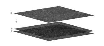
Figure 1: Images samples of the stack. The stack is used to predict a ground scene reference image.

As a result, we obtain a true image of the ground scene illuminated by multi-pass.

Once the predicted image is available, it can be used, for example, as a reference image for change detection. In this case, the changes of the ground scene before the first pass and the latter passes can be detected. To evaluate this proposal, we performed a simple processing sequence for the stack of images including ground estimation, change detection and change classification, as shown in Figure 2.

The stack of images is used as input of the AR model, which provides a ground reference image. Then, each image used in the stack is compared to the reference image, resulting in difference images. The processing is followed by thresholding given rise to a binary image. The last processing step is reserved for morphological operations such as erosion and dilation. For the experiments, we performed an erosion followed by a dilatation.

The measures of performance of change detection is based on the probability of detection ($\text{P}_{d}$) and false alarm rate (FAR). The quantity $\text{P}_{d}$ is obtained from the ratio between the number of detected targets and the total numbers of known targets, and FAR is defined by the number of false alarms detected per square kilometer [10].

Figure 2: Processing scheme for change detection.

4 Experimental results

In this section we provide some experimental results to assess the performance obtained by the processing scheme presented in Section 3 by considering predicted images as ground estimation input.

4.1 Data description

The data used for this study were delivered by CARABAS II [10], a Swedish ultra-wideband VHF SAR system. The data included eight images with almost identical flight geometry, but with four different targets deployments in the ground scene [15, 10]. All information about the data can be found in [15, 10]. In this paper, we consider the image stack generated by passes five and six and missions one to four for each pass. Figures 3 and 4 present eight CARABAS II images forming the image stack used in the AR model. Each image is represented by a matrix of $3000\times 2000$ pixels, corresponding to an area of $6\leavevmode\nobreak\ \text{km}^{2}$. The ground scene is dominated by forest with pine trees. Fences, power lines and roads were also present in the scene. Some military vehicles were deployed in the SAR scene and placed in a manner to facilitate their identifications in the tests [10]. The targets can be seen in the upper-left corner in Figures 3(a), 3(b), 4(a), and 4(b); and in the lower-right corner in Figures 3(c), 3(d), 4(c), and 4(d). In Figures 3 and 4 it is possible to identify the targets and other structures, like roads and power lines. Each image has $25$ targets with three different sizes [10].

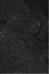
(a) Mission one

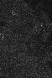
(b) Mission two

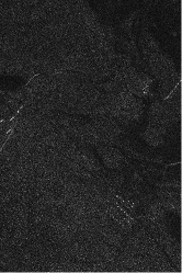
(c) Mission three

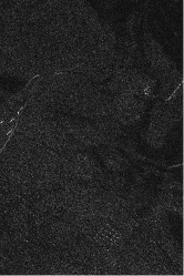
(d) Mission four

Figure 3: CARABAS II images for pass five.

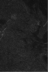
(a) Mission one

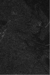
(b) Mission two

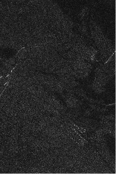
(c) Mission three

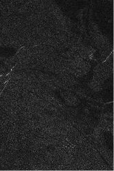
(d) Mission four

Figure 4: CARABAS II images for pass six.

4.2 Ground estimation

In this study we considered the AR model presented in Section 2. The resolution of the CARABAS II system is approximately $3\times 3\;\text{m}^{2}$. Since a pixel represents a $1\times 1\;\text{m}^{2}$, considering an one-dimensional model, the closest pixels will be more correlated than the others. Thus, we used $p=1$ in the AR models. Based on the fitted model, we obtained the forecast of one step ahead for each pixel, like showed in Equation (2). This forecasting provides a new image presented in Figure 5 representing the ground estimation of the SAR scene.

We can visually compare the images considered for the ground estimation (showed in Figures 3 and 4), and the ground estimation (the new image presented in Figure 5). Hence, we can verify the lake regions, the forest, and strong scatters in all images. However, the deployed vehicles in the missions, that can be verified in different locations in Figures 3 and 4, do not appear in Figure 5. With visual verification, Figure 5 seems to present a good estimation of the ground scene.

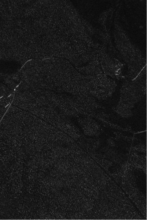
Figure 5: Prediction image of the AR$(1)$ model.

Figure 6 presents the image with the absolute estimative values of the autoregressive terms of the AR$(1)$ model. The black points in the image correspond to the lowest values. It is possible to see (in the boxes) the regions where the vehicles were deployed in some instants in time more highlighted than the other structures in the image. Thus, the AR model reduce the amplitude of the targets in the ground estimation. In future studies, this image can be used to indicate the changes in the ground scene.

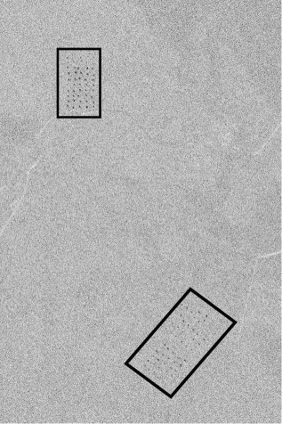
Figure 6: Absolute values of the autoregressive terms estimated by the AR$(1)$ model. The black points correspond to the lowest values.

Figures 7 and 8 present the images obtained by the subtraction between the image of interest and the ground estimation image obtained by the AR$(1)$ model. We can see that the deployed vehicles are more highlighted in Figures 7 and 8. Only in Figure 7(b) we can verify the strong scatters in the greater prominence. In all other images, the strong scatters were almost completely removed.

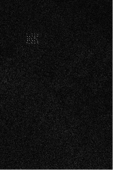
(a) Mission one

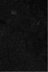
(b) Mission two

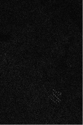
(c) Mission three

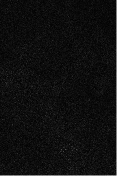
(d) Mission four

Figure 7: Difference images for pass five.

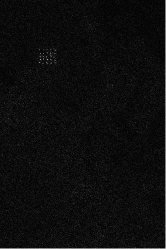
(a) Mission one

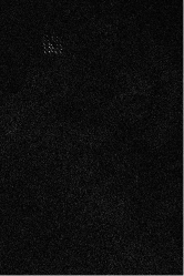
(b) Mission two

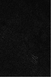
(c) Mission three

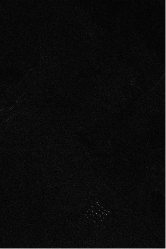
(d) Mission four

Figure 8: Difference images for pass six.

4.3 Application in change detection

We consider CDA as an application to the obtained ground estimation. The change detection is realized according to the processing scheme presented in Figure 2. The AR model gives the ground estimation presented in Figure 5. With the estimated image of the ground scene, we performed subtractions between the interest images and the obtained images as given in Figures 7 and 8. The next step is reserved for thresholding and morphological operations to obtain the change detection results. Figure 9 presents the histogram for Figure 7(a). We can see that the magnitude distribution of the images obtained by the subtraction between the interest image and the ground estimation image is approximately a normal distribution.

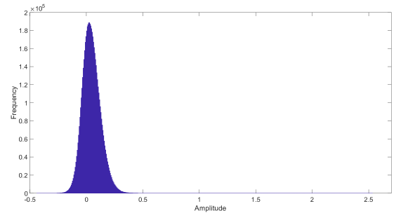
Figure 9: Histogram for Figure 7(a).

Thus, the thresholding can be choosing as

$$C=\frac{\lambda-\widehat{\mu}}{\widehat{\sigma}},$$

where $C$ is the detection constant, $\widehat{\mu}$ is the mean, and $\widehat{\sigma}$ the standard deviation of the considered pixels in the image stack. For evaluation, the values $4.5;5;5.5;6;6.5$ are selected for $C$.

Table 1 presents the change detection results for $C=4.5$. We detect $188$ deployed vehicles with $33$ false alarms, i.e., the detection probability is $94\%$ while the false alarm rate is only $0.69/\text{km}^{2}$. In these same images, in [10], it was detected $188$ vehicles with $52$ false alarms. Hence, considering the AR model to estimate the ground scene, we obtained the same number of detected vehicles with less $19$ false alarms than [10].

Especially, the change detection results for mission four and pass five is two false alarms in comparison to $29$ in [10] (one less detection). Among the $33$ false alarms presented in Table 1, $24$ of them are related to the images in Figures 7(b) and 8(d). Other approaches to ground estimation and other values of $p$ can be further investigated to provide more accurate predicted SAR images.

Figure 10 presents the ROC curve [12] of the change detection results, showing the probability of detection versus the false alarm rate for different values of threshold. We can observe in the ROC curve values of $\text{P}_{d}=0.92$ with $\text{FAR}=0.42$ or $\text{P}_{d}=0.90$ with $\text{FAR}=0.35$, as examples.

Table 1: Change detection results obtained with $C=4.5$

Case of Interest		Number of	Detected	$\text{P}_{d}$	Area	Number of	FAR
Mission	Pass	known targets	Targets		$[\text{Km}^{2}]$	false alarms
$1$	$5$	$25$	$25$	$1.00$	$6$	$0$	$0.00$
$2$	$5$	$25$	$16$	$0.64$	$6$	$9$	$1.50$
$3$	$5$	$25$	$25$	$1.00$	$6$	$1$	$0.17$
$4$	$5$	$25$	$22$	$0.88$	$6$	$2$	$0.33$
$1$	$6$	$25$	$25$	$1.00$	$6$	$1$	$0.17$
$2$	$6$	$25$	$25$	$1.00$	$6$	$2$	$0.33$
$3$	$6$	$25$	$25$	$1.00$	$6$	$3$	$0.50$
$4$	$6$	$25$	$25$	$1.00$	$6$	$15$	$2.50$
Total		$200$	$188$	$0.94$	$48$	$33$	$0.69$

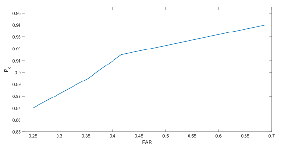
Figure 10: ROC curve obtained with the proposed method, for $C_{i}$, $i=4.5,\,5,\,5.5,\,6,\,6.5$.

5 Conclusion

Usually, AR models are used in the study of data that are defined in the time domain. In this paper we proposed the use of an AR$(1)$ model for a stack of eight SAR images to retrieve a ground scene estimation. By using this technique, it was possible to obtain a reliable representation of the ground scene, which could be used as a reference image in a change detection algorithm. We applied subtractions between the ground estimation image obtained by AR models and the interest images. With simple thresholding and morphological operations, we obtained competitive results of $\text{P}_{d}$ and FAR when compared to the results presented in [10].

To the best of our knowledge, this is the first treatment for ground estimation with image stack by using AR models. In future studies, we intend to use stacks with more images generating possibly more accurate adjustments and consequently more reliable forecasts or more accurate ground estimation.

References

- [1] L. W. Biscainho, AR model estimation from quantized signals, IEEE Signal Processing Letters, 11 (2004), pp. 183–185.
- [2] G. Box, G. M. Jenkins, and G. Reinsel, Time series analysis: forecasting and control, Hardcover, John Wiley & Sons, June 2008.
- [3] P. J. Brockwell and R. A. Davis, Time series: theory and methods, Springer, 2013.
- [4] , Introduction to time series and forecasting, Springer, 2016.
- [5] K. Folkesson, G. Smith-Jonforsen, and L. M. Ulander, Model-based compensation of topographic effects for improved stem-volume retrieval from CARABAS-II VHF-band SAR images, IEEE Transactions on Geoscience and Remote Sensing, 47 (2009), pp. 1045–1055.
- [6] T. Ghirmai, Representing a cascade of complex Gaussian AR models by a single Laplace AR model, IEEE Signal Processing Letters, 22 (2015), pp. 110–114.
- [7] S. M. Kay, Fundamentals of Statistical Signal Processing. Estimation theory, Volume I, Prentice Hall, 1993.
- [8] , Fundamentals of Statistical Signal Processing. Detection Theory, Volume II, Prentice Hall, 1998.
- [9] B. Liu, V. G. Reju, and A. W. Khong, A linear source recovery method for underdetermined mixtures of uncorrelated AR-model signals without sparseness, IEEE Transactions on Signal Processing, 62 (2014), pp. 4947–4958.
- [10] M. Lundberg, L. M. Ulander, W. E. Pierson, and A. Gustavsson, A challenge problem for detection of targets in foliage, in Algorithms for Synthetic Aperture Radar Imagery XIII, International Society for Optics and Photonics, 2006.
- [11] R. Machado, V. T. Vu, M. I. Pettersson, P. Dammert, and H. Hellsten, The stability of UWB low-frequency SAR images, IEEE Geoscience and Remote Sensing Letters, 13 (2016), pp. 1114–1118.
- [12] C. E. Metz, Basic principles of ROC analysis, in Seminars in nuclear medicine, vol. 8, Elsevier, 1978, pp. 283–298.
- [13] P. Milenkovic, Glottal inverse filtering by joint estimation of an AR system with a linear input model, IEEE Transactions on Acoustics, Speech, and Signal Processing, 34 (1986), pp. 28–42.
- [14] L. Ulander, A. Gustavsson, J. Fransson, M. Magnusson, G. Smith-Jonforsen, K. Folkesson, B. Hallberg, and L. Eriksson, Mapping of wind-thrown forests using the VHF-band CARABAS-II SAR, in IEEE International Symposium on Geoscience and Remote Sensing, IEEE, 2006, pp. 3684–3687.
- [15] L. M. Ulander, M. Lundberg, W. Pierson, and A. Gustavsson, Change detection for low-frequency SAR ground surveillance, IEE Proceedings-Radar, Sonar and Navigation, 152 (2005), pp. 413–420.
- [16] L. M. Ulander, W. E. Pierson, M. Lundberg, P. Follo, P.-O. Frolind, and A. Gustavsson, Performance of VHF-band SAR change detection for wide-area surveillance of concealed ground targets, in Algorithms for Synthetic Aperture Radar Imagery XI, vol. 5427, International Society for Optics and Photonics, 2004, pp. 259–271.
- [17] V. T. Vu, Wavelength-resolution SAR incoherent change detection based on image stack, IEEE Geoscience and Remote Sensing Letters, 14 (2017), pp. 1012–1016.