Conditions for Oscillator Small-Signal Amplitude-Phase Orthogonality.

Abstract

The paper explores a previously unknown connection relating the symmetry properties of an oscillator steady-state to the orthogonal representation of amplitude and phase variables in the small-signal regime. It is shown that only circuits producing perfectly symmetric steady-states can produce an orthogonal Floquet decomposition. Considering room temperature operation this scenario implies zero AM-PM noise conversion. This surprising and novel result follows directly from the predictions of a rigorous model framework first described herein. The work presented in this text extend the current state-of-the-art w.r.t. oscillator small-signal/noise characterization.

Keywords oscillators, phase noise, AM-PM noise conversion, circuit analysis, nonlinear dynamical systems, system analysis and design

1 Introduction

The oscillator small-signal/linear-response (LR) governs the circuit dynamics in reply to small perturbations, e.g. noise, around the periodic steady-state (PSS). Rigorous methods for characterizing oscillator dynamics in a noisy environment are absolutely critical for developing analysis/synthesis tools used to optimize performance of various critical circuits found in modern communication systems.

In the general case, small-signal oscillator amplitude and phase variables are defined in-terms of mutually oblique (i.e. non-orthogonal) Floquet vectors decomposing the LR map [1, 2, 3, 4]. One important implication of this oblique representation is the integration of amplitude-noise into oscillator phase response; a process known as oscillator AM-PM noise conversion[5, 6, 7, 8, 9, 10, 11, 12, 13, 14, 15]. The aim of the model described herein is to seek an answer to the open question :what type of oscillators support a fully orthogonal small-signal representation implying zero AM-PM ? This scenario is represented mathematically in-terms of an orthogonal Floquet decomposition (OFD) of the LR. The topic was previously briefly studied by the authors in [15], however, only for the special case of planar oscillator and strictly from a simulation-based perspective.

The paper documents and validates the novel SYM-OFD model framework with specific focus paid to the remarkable statement : ${\text{ORTHOGONALITY (OFD)}\Rightarrow}$ STEADY-STATE SYMMETRY. This statement is both notable and unanticipated. To our knowledge, this constitutes the first ever description of a direct analytical link relating a specific decomposition of the oscillator LR and the properties of the underlying PSS. The statement also provides a formal sufficient condition for zero AM-PM noise conversion in higher dimensional oscillators. This relation cannot be reached using arguments based on empirical or phenomenological reasoning but relies on the rigorous methodology developed herein. It is important to note that the above statement references a strict one-way relation i.e. an orthogonal LR representation implies symmetry. The reverse implication is however not true as symmetry does not imply orthogonality.

The validity of the orthogonal model representation has been debated in the literature for several decades (see e.g. [1, 16, 3, 4, 9, 10]). Unlike the natural Floquet description, an orthogonal model representation is, in the general case, artificial(un-natural) meaning that is coordinate dependent which implies that corresponding model operators will not represent tensors. This issue has important implications for oscillator LR modelling. A coordinate-independent/tensor approach, by definition, always leads to simplest, cleanest and most generalized model description [4]. Our work herein provides a definitive resolution of the aforementioned open debate : in-order for a orthogonal modelling approach to be valid (i.e. be natural, coordinate-independent) the underlying PSS must be symmetric (orthogonality implies symmetry).

In answering these types of open question, using a rigorous, proof-based, methodology, the novel SYM-OFD framework advances the current state-of-the-art w.r.t. time-domain oscillator small-signal/noise characterization and modelling. It introduces several novel ideas and insights such as e.g. why OFD’s are not observed in real-life oscillator descriptions where non-linear device-models make it impossible to attain perfect PSS symmetry. Finally, the methodology enables a whole new category of numerical optimization tools which could potentially find use in future applications.

In-order to briefly explore the last point, consider e.g. a scenario where some oscillator figure-of-merit (FoM), describing a particular performance metric of interest, attains an optimum at an OFD state. We introduce two strictly positive scalars, $\Lambda,\Upsilon$, which measure the deviation from PSS symmetry, and OFD solution state, respectively, with $\Upsilon=0,\Lambda=0$ corresponding to perfect symmetry/OFD (see section 6.1). In the vicinity of zeros for these two measures, the theory then predicts that $\Upsilon$ (orthogonality) will be minimized alongside $\Lambda$ (symmetry) i.e. $\Upsilon\to 0\Rightarrow\Lambda\to 0$. Using standard minimization routines[17], $\min(\Lambda)$ is then derived, starting from a given initial condition in parameter-space. If parameter sets, achieving a set $\Upsilon$ goal, indeed exist then the SYM-OFD methodology guarantees that at-least one of these can be found in the vicinity of equivalent symmetry (zero) points. Due to the one-way nature of the orthogonality/symmetry relation there will be the possibility of false-positives (symmetry point may imply a non-OFD state). However, even with this serious drawback, the scheme proposed here is easily several orders-of-magnitudes faster than any competing approach. The idea discussed here is only possible due to the connections forged by the SYM-OFD framework. It is simply not possible to directly optimize/minimize the OFD measure, $\Upsilon$, given that the LR equations are unknown a-priori to calculating the PSS.

2 Detailed paper summary & main result.

Section 3 starts with a quick introduction to some basic underlying topics (tangent-bundle, Floquet theory, OFD oscillators etc.). The analysis in the next two sections, leading up to the main result in theorem 5.1, can then be divided into $4$ consecutive steps (refer to acronym/symbol lists in back of paper) :

1. Sections 4 and 4.1 : A normal-form oscillator (NF-OSC), $\mathbf{o}=(\psi_{\tau},\xi)$, on the domain $\mathbb{U}$, is used to parameterize the oscillator under investigation, $\mathbf{q}=(\phi_{\tau},\gamma)$, on domain $\mathbb{W}_{s}$ (see figs. 3 and 5). This parametrization is facilitated in-terms of a unique conjugation-map, $h:\mathbb{U}\to\mathbb{W}_{s}$, where $h$ conjugates $\mathbf{o}$ and $\mathbf{q}$; written $\mathbf{o}\sim_{h}\mathbf{q}$. Conjugation preserves invariant sets and specifically $h(\xi)=\gamma$.

2. Section 4.2 : The NF-OSC, $\mathbf{o}$, is chosen according to the two criteria : it must have a canonical (simple) model description and it must be a OFD oscillator ($\mathbf{o}\in\mathbf{O}^{\perp}$). The chosen model is given the handle PNF-OSC. It is shown that PNF-OSC limit-cycle is perfectly symmetric $\xi\in\mathcal{SYM}_{n}$.

3. Section 4.3 : Let $\mathbf{o}\sim_{h}\mathbf{q}$, where, $\mathbf{o}\in\mathbf{O}^{\perp}$, is the PNF-OSC developed in step #2 above. The demand, $\mathbf{q}\in\mathbf{O}^{\perp}$, restricts the conjugation map as $h\in\mathbf{H}_{C}\subset\mathbf{H}$ (see proposition 4.3 & symbol list). In summary : let $\mathbf{q}$ be conjugate to the PNF-OSC, then, $\mathbf{q}\in\mathbf{O}^{\perp}$, will hold if, and only if, $h\in\mathbf{H}_{C}$. A new conjugation operator (equivalence relation), $\overset{c}{\sim}_{h}$, is introduced and the above statement is written (see proposition 4.4) as $\mathbf{q}\in\mathbf{O}^{\perp}\Leftrightarrow\mathbf{o}\overset{c}{\sim}_{h}\mathbf{q}$.

4. Proposition 5.2 : Using Liouville’s and Schottkys theorems [18, 19, 20, 21, 22, 23] it is shown that the conjugation map, $h\in\mathbf{H}_{C}$, must have the form $h(y)=\rho Ay$ where $\rho\in\mathbb{R}\setminus\{0\}$ is a non-zero real value and $A\in O(n)$ is an orthogonal $n\times n$ matrix.

5. Theorem 5.1 : The result is reached by following the chain of steps #1-#4 described above : #1 ($h(\xi)=\gamma$) $\to$ #2 ($\xi\in\mathcal{SYM}_{n}$) $\to$ #3 ($h\in\mathbf{H}_{C}$) $\to$ #4 ($h(y)=\rho Ay$) which allows the calculation $\gamma=h(\xi)=A\xi\in\mathcal{SYM}_{n}$ where $A\xi\in\mathcal{SYM}_{n}$ holds because multiplication by the orthogonal map $A$ preserves the symmetry of $\xi$ (i.e. maps $\mathcal{SYM}_{n}\to\mathcal{SYM}_{n}$). At this point we have reached the main result (theorem 5.1) : $\mathbf{q}\in\mathbf{O}^{\perp}\Rightarrow\gamma\in\mathcal{SYM}_{n}$ which, in words, says that only oscillators with a perfectly symmetric limit-cycle support an OFD $({\text{ORTHOGONALITY}\Rightarrow\text{STEADY-STATE SYMMETRY}})$. Please note that the above statement is a strict one-way relation.

Finally, it is proven in section 5.1 that the analysis results, carried out using the specific PNF-OSC model, are in-fact unique. As discussed in section 5.1 this follows straight from the fact that, $\overset{c}{\sim}$, represents an equivalence relation. Section 6 details a series of numerical experiment, spanning several different oscillator circuits, all of which, unequivocally, support the claim introduced in theorem 5.1.

2.1 Summary of methodology

Consider fig. 5 which shows the PNF-OSC parameterizing an unspecified oscillator circuit; i.e. the N-OSC. The dynamics of the PNF-OSC circuit is illustrated in fig. 4 which shows transient orbits plus the limit-cycle of this circuit. This oscillator circuit is designed to be an OFD oscillator and we find that the limit-cycle is symmetric. The N-OSC circuit in fig. 5, could be any hyperbolic $n$-dimensional oscillator e.g. one of the circuits described in section 6. The parametrization map, $h$, transforming the PNF-OSC orbits into N-OSC orbits (and vice-versa through $h^{-1}$) is guaranteed to exist and to be unique (see section 4). This transformation preserves invariant spaces and hence maps the PNF-OSC limit-cycle into the equivalent N-OSC set (see fig. 5 caption).

A conjugation-map, $h$, relating two OFD oscillators, must belong to the special subset of maps $\mathbf{H}_{C}$ (propositions 4.3 and 4.4). Hence, only a special type of map can transform between two OFD oscillators. The PNF-OSC is, by design, an OFD oscillator and it follows that the N-OSC (righthand-side of fig. 5) will be an OFD as well if, and only if, $h$ belongs to the set $\mathbf{H}_{C}$. So now it becomes clear why the PNF-OSC was chosen as an OFD oscillator. We are trying to describe the subset of all N-OSC circuits which are also OFD oscillators. This then means that both the PNF-OSC and N-OSC will be OFD circuits which then automatically restricts the possible conjugation/parametrization-map candidates from any smooth map, $h\in\mathbf{H}$, to the much smaller subset $h\in\mathbf{H}_{C}\subset\mathbf{H}$. This analysis trick proves fruitful as we are able to partially characterize this smaller subset of maps (see section 5). Specifically, the theory shows that a map in $\mathbf{H}_{C}$ transform the limit-cycles in fig. 5 in-terms of simple linear orthogonal map (scalar scaling + rotation + inversion). This map preserves symmetry and the N-OSC limit-cycle will hence also be symmetric. This last statement is the main result of this paper, i.e. theorem 5.1, which represents a strict one-way relation (see footnote 5.)

The question of uniqueness of this result, derived using the specific PNF-OSC model, becomes important to discuss. Why can we not just chose some other OFD model, call it XNF-OSC, perhaps even with a non-symmetric limit-cycle and then produce a completely different conclusion? As explained in section 5.1, the uniqueness of theorem 5.1 is saved by fact that conjugation (parametrization) represents an equivalence relation. Basically, if the XNF-OSC parameterizes the N-OSC then it must also parameterize the PNF-OSC and vice-versa (via inverse map) which then implies that the XNF-OSC (an OFD oscillator) must have a symmetric limit-cycle (see above discussion). Hence, whether we parameterize the N-OSC in fig. 5 using the PNF-OSC, the XNF-OSC, or any other possible OFD template, is irrelevant. We will always arrive at the same result in theorem 5.1.

3 Basic theory

The oscillator state is governed by a $n$-dimensional vector-field $f:\mathbb{R}^{n}\to\mathbb{R}^{n}$ generating a set of $n$ coupled ordinary differential equations (ODE) $\dot{x}=f(x)$ with $x(t):\mathbb{R}\to\mathbb{R}^{n}$ being the $n$-dimensional state-vector parameterized by time $t$. The solution, corresponding to the initial condition $x(0)=x_{0}$ is written $x(t)=\phi_{t}(x_{0})$ with $\phi_{t}:\mathbb{R}\times\mathbb{R}^{n}\to\mathbb{R}^{n}$ known as the flow. The oscillator DC-point (quiescent start-up point), $x_{q}$, is a zero-point of the vector field $f(x_{q})=0$ and hence a fixed-point of the flow $\phi_{t}(x_{q})=x_{q}$ for all $t$. The oscillator ODE generates a hyperbolic $1$-dimensional attractor, $\gamma$, known as a limit cycle. The oscillator PSS, $x_{s}(t+T)=x_{s}(T)$ is then a $T$-periodic orbit, corresponding to an initial condition in $\gamma$, i.e. $x_{s}(t)=\psi_{t}(x_{0})$ with $x_{0}\in\gamma$. Herein, the ODE description is assumed time-normalized using the time-scale $\tau=2\pi(t/T)$ which results in a $2\pi$ periodic limit-cycle solution $x_{s}(\tau+2\pi)=x_{s}(\tau)$ corresponding to an oscillator frequency $\omega_{0}=2\pi/T=1$. The term, oscillator $\mathbf{q}$, refers herein to the solution pair $\mathbf{q}=(\phi_{\tau},\gamma)$.

3.1 The stable manifold & isochrone foliation

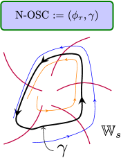
Figure 1: A hyperbolic $n$-dimensional oscillator $\mathbf{q}=(\phi_{\tau},\gamma)$, i.e. a N-OSC, and the isochrone foliation of the stable manifold $\mathbb{W}_{s}(\gamma)$. The purple curves represent $4$ leaves in the foliation of $\mathbb{W}_{s}(\gamma)$ (see eq. 1). The blue and orange curves represent orbits of $\phi_{\tau}$ which approach $\gamma$ asymptotically with time.

We consider a $n$-dimensional, hyperbolically stable, oscillator (N-OSC), $\mathbf{q}=(\phi_{\tau},\gamma)$, with PSS $x_{s}(\tau)=x_{s}(\tau+2\pi)$ (time-normalized). The oscillator stable manifold defines the connected subset of $\mathbb{R}^{n}$ containing all initial conditions which converge towards the oscillator limit-cycle asymptotically with time $\lim_{\tau\rightarrow\infty}|\phi_{\tau}(x_{0})-\gamma|\rightarrow 0$ for   $x_{0}\in\mathbb{W}_{s}$. The text herein considers electrical oscillators with a single DC/start-up point, $x_{q}$, assumed to lie at the origin which produces a stable manifold consisting of $\mathbb{R}^{n}$ minus the origin i.e. $\mathbb{W}_{s}=\mathbb{R}^{n}\setminus\{0\}$.

It is a well-established fact[24, 25, 4] that an open subset $\mathbb{W}_{s}(\gamma)\subset\mathbb{W}_{s}$ of this manifold, known as the stable manifold of $\gamma$ (dimension $\geq n-2$), can be foliated by continuum of $(n-1)$-dimensional hyper-surfaces known as isochrones i.e. equal time/phase sets

$$\mathbb{W}_{s}(\gamma)=\underset{\eta\in[0,2\pi)}{\bigcup}\bigl{\{}\mathcal{I}_{\eta}\bigr{\}}$$ (1)

where each leaf, $\mathcal{I}_{\eta}$, of this foliation contain points in $\mathbb{W}_{s}(\gamma)$ with asymptotic oscillator phase $\eta$. The topics discussed above are illustrated schematically in fig. 1.

3.2 Floquet theory & the oscillator tangent-bundle

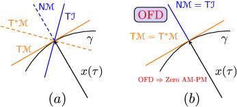
Figure 2: (a) : the decomposition of the tangent-bundle $\mathsf{T}_{\gamma}\mathbb{R}^{n}=\mathsf{T}\mathcal{M}\oplus\mathsf{T}\mathcal{I}$ (limit-cycle/isochrone tangent spaces,solid line) and corresponding dual tangent-bundle $\mathsf{T}_{\gamma}^{*}\mathbb{R}^{n}=\mathsf{T}^{*}\mathcal{M}\oplus\mathsf{N}\mathcal{M}$ (dashed line). This construct, based on the geometric notion of an isochrone foliation of $\mathbb{W}_{s}(\gamma)$ (see fig. 1). (b) : the orthogonal Floquet decomposition (OFD) $\mathsf{T}_{\gamma}\mathbb{R}^{n}\in\mathbf{B}^{\perp}$. For an orthogonal system the distinction between basis and dual basis is erased.

The N-OSC, $\mathbf{q}=(\phi_{\tau},\gamma)$, introduced above, is hyperbolic and a unique corresponding set of $n$ (dual) Floquet vectors $\{u_{i}(\tau),v_{i}(\tau)\}_{i=1}^{n}:\mathbb{R}\to\mathbb{R}^{n}$, are then known to exist [1, 2, 11, 4]. These objects obey the bi-orthogonality condition (ODE systems) $(v_{i}(\tau),u_{j}(\tau))=\delta_{ij}\,\text{for}\,i=1,2,\cdots n$ where $(\cdot,\cdot)$ designates the inner Euclidian product and $\delta_{ij}$ is the Kroenecker delta-function.

The fundamental-matrix map (F-MATRIX), $d\phi_{\tau}:\mathbb{R}\times\mathbb{R}^{n}\to\mathbb{R}^{n\times n}$, is derived by linearizing the full flow, $\phi_{\tau}$, around the limit-cycle, $\gamma$. This map describes the oscillator linear-response (LR) and hence governs orbits generated by weak perturbations around $x_{s}(\tau)\in\gamma$. It can be decomposed as $d\phi_{\tau}=\sum_{j=1}^{n}\exp(\mu_{j}\tau)u_{j}(\tau)v_{j}^{\top}(0)$ where $\mu_{i}$ is the time-normalized characteristic Floquet exponent corresponding to $i$th (dual) Floquet vectors[2, 4]. It follows directly that $u_{i}(0){=}u_{i}(2\pi)$ is an eigenvector of the special F-MATRIX, $d\phi_{2\pi}=\sum_{j=1}^{n}\exp(2\pi\mu_{j})u_{j}(2\pi)v_{j}^{\top}(0)$, known as the Monodromy Matrix (M-MATRIX), with corresponding eigenvalue $\lambda_{i}=\exp(2\pi\mu_{i})$ being the $i$th Floquet characteristic multiplier. Oscillator stability demands $\Re\{\mu_{i}\}\leq 0$ (real part $\leq 0$) for all $i$. Henceforth, the triple $\{u_{i}(\tau),v_{i}(\tau),\mu_{i}\}$, or individual constituents of this triple, will be referred to as the $i$th (Floquet) mode. The dynamics of the circuits considered herein are real and modes hence must appear in conjugate pairs (i.e. $u_{i}=u_{i+1}^{*}$) with real modes (i.e. modes with zero imaginary parts) appearing as singles. For oscillator solutions a special phase-mode, $\{u_{1}(\tau),v_{1}(\tau),\mu_{1}=0\}$, is known to exist, describing the neutrally stable dynamics tangential to the limit-cycle $\gamma$. The associated dual vector, $v_{1}$, is known as the perturbation-projection-vector (PPV) [2, 26]. It can be readily shown that $u_{1}$ is proportional to $\dot{x}_{s}$ and we fix $u_{1}(\tau)=\dot{x}_{s}(\tau)$ [1, 2, 11, 4].

3.2.1 The oscillator tangent-bundle

For a hyperbolic solution, the Floquet collection $\{u_{i}(\eta)\}$, constitute a complete set and hence form a basis for $\mathbb{R}^{n}$. The origin of this vector-space is the PSS point, $x_{s}(\eta)$. This translated vector-space is known as the tangent-space $\mathsf{T}_{\eta}\mathbb{R}^{n}=\text{span}\{u_{1}(\eta),u_{2}(\eta),\cdots u_{n}(\eta)\}$ at $x_{s}(\eta)$. The disjoint union of all these tangent-spaces, one for each point on the PSS $x_{s}(\tau)=x_{s}(\tau+2\pi)\in\gamma$, is then is known as the (oscillator) tangent-bundle

$$\mathsf{T}_{\gamma}\mathbb{R}^{n}=\underset{\eta\in[0,2\pi)}{\bigcup}\mathsf{T}_{\eta}\mathbb{R}^{n}=\text{span}\{u_{1}(\eta),u_{2}(\eta),\cdots u_{n}(\eta)\}$$ (2)

Both the limit-cycle and isochrone foliation (see fig. 1) are invariant sets under the flow which then directly implies the following bundle representation $\mathsf{T}_{\gamma}\mathbb{R}^{n}=\mathsf{T}\mathcal{M}\oplus\mathsf{T}\mathcal{I}$ and from [4], $\mathsf{T}\mathcal{M}=\cup\mathsf{T}_{\eta}\mathcal{M}=\text{span}\{u_{1}(\eta)\}$, $\mathsf{T}\mathcal{I}=\cup\mathsf{T}_{\eta}\mathcal{I}=\text{span}\{u_{2}(\eta),u_{3}(\eta),\cdots u_{n}(\eta)\}$ with $\eta\in[0,2\pi)$. The special mode, $u_{1}(\tau)$, spanning $\mathsf{T}\mathcal{M}$, is the so-called phase-mode whereas the set $\{u_{i>1}(\tau)\}$ are the $(n-1)$ amplitude-modes. Repeating the above discussion for the adjoint F-MATRIX we can derive the oscillator dual tangent-bundle $\mathsf{T}^{*}_{\gamma}\mathbb{R}^{n}{=}\text{span}\{v_{1}(\eta),v_{2}(\eta),\cdots v_{n}(\eta)\}$ which is decomposed as $\mathsf{T}_{\gamma}^{*}\mathbb{R}^{n}=\mathsf{T}^{*}\mathcal{M}\oplus\mathsf{N}\mathcal{M}$ where $\mathsf{T}^{*}\mathcal{M}=\text{span}\{v_{1}(\tau)\}$ (the PPV bundle) and $\mathsf{N}\mathcal{M}=\text{span}\{v_{2}(\tau),v_{3}(\tau),\cdots v_{n}(\tau)\}$ [4].

Let $\mathbf{B}$ be the set of all possible tangent-bundles of the form in eq. 2. The subset, $\mathbf{B}^{\perp}\subset\mathbf{B}$, then hold all orthogonal bundle decompositions, or more specifically, all orthogonal Floquet decomposition (OFD)

$$\mathbf{B}^{\perp}=\bigl{\{}\mathsf{T}_{\gamma}\mathbb{R}^{n}\in\mathbf{B}:\,\,u_{k}(\tau)\perp u_{j}(\tau)\,\,\text{for}\,\,k\neq j\,\,,\,\forall\tau\bigr{\}}$$ (3)

where $\perp$ and $\forall$ are mathematical symbols for orthogonal and for all. Let $\mathbf{O}$ be the set of all hyperbolic, stable oscillators. The subset $\mathbf{O}^{\perp}\subset\mathbf{O}$, then contain the special OFD oscillators

$$\mathbf{O}^{\perp}=\bigl{\{}\,\mathbf{q}=(\phi_{\tau},\gamma)\in\mathbf{O}\,:\,\mathsf{T}_{\gamma}\mathbb{R}^{n}\in\mathbf{B}^{\perp}\,\bigr{\}}$$ (4)

thus $\mathbf{O}^{\perp}$ hold all the oscillators with a tangent bundle in $\mathbf{B}^{\perp}$. The concepts discussed here are illustrated in fig. 2.

Consider a noise signal $\varrho(\tau):\mathbb{R}\to\mathbb{R}^{n}$, perturbing the oscillator PSS. In order to facilitate a discussion of AM-PM noise conversion, an orthogonal frame $\{e_{j}(\tau)\}_{i=1}^{n}$, moving over (i.e. with origin at) $x_{s}(\tau)$, is introduced with $e_{1}(\tau)$ being tangent to $\gamma$ implying $e_{1}(\tau)\parallel u_{1}(\tau)$. The remaining $n-1$ components $\{e_{j}(\tau)\}_{i=2}^{n}$, all correspond to directions orthogonal to $\gamma$ and can then viewed as contra-variant versions of the set $\{v_{j}(\tau)\}_{i=2}^{n}$ spanning $\mathbb{NM}$ (see fig. 2). The noise-signal is then decomposed as $\varrho(\tau)=\text{PM-noise + AM-noise}=a_{1}(\tau)e_{1}(\tau)+\sum_{i=2}^{n}a_{i}(\tau)e_{i}(\tau)$. Note, that we are free to decompose the noise using any frame. The calculated phase-noise spectrum is unaffected. The Floquet frame is only inherent to the oscillator LR itself not to any perturbing signal. From the bi-orthogonality condition $(v_{i}(\tau),u_{j}(\tau))=\delta_{ij}$, discussed above, together with the OFD oscillator definition in eqs. 3 and 4, the phase-mode $u_{1}$ and PPV $v_{1}$ must be parallel, $u_{1}(\tau)\parallel v_{1}(\tau)$, for all $\tau$ (see also fig. 2.b). In this OFD scenario, the PPV hence only collects noise along $u_{1}\propto\dot{x}_{s}$, and there will hence be no integration of AM-noise (as defined herein) into the phase of the oscillator which is the definition of zero AM-PM noise conversion.

Remark 3.1.

An OFD oscillator, $\mathbf{q}\in\mathbf{O}^{\perp}$, has zero AM-PM noise conversion.

4 Topological conjugate oscillators

We consider the two $n$-dimensional open sets $\mathbb{U}=\mathbb{W}_{s}=\mathbb{R}^{n}\backslash\{0\}$ parameterized by coordinates $y=(y_{1},y_{2},\cdots,y_{n})$ and $x=(x_{1},x_{2},\cdots,x_{n})$, respectively. Here $\mathbb{W}_{s}$ is the stable manifold for the N-OSC, $\mathbf{q}=(\phi_{\tau},\gamma)$, generated by the ODE $\dot{x}=f(x)$. The new domain, $\mathbb{U}$, known herein as the parametrization manifold, is the stable-manifold of the normal-form oscillator (NF-OSC), $\mathbf{o}=(\psi_{\tau},\xi)$, generated by the ODE $\dot{y}=g(y)$.

The theory of topological conjugate flows [27, 28, 29, 30, 31, 32], loosely speaking, describes a scenario wherein the NF-OSC, $\mathbf{o}$, on $\mathbb{U}$, is used to parameterize the N-OSC, $\mathbf{q}$, on $\mathbb{W}_{s}$. The idea is to construct a canonical (simple) model on $\mathbb{U}$ and then perform all analysis on this simplified representation. This concept is akin to applying a basis change in standard linear-algebra in-order to simplify solution procedure. The setup discussed here is fully symmetric, ($\mathbb{U}=\mathbb{W}_{s}$), which implies that $\mathbf{q}$ on $\mathbb{W}_{s}$ can equally well be said to parameterizes $\mathbf{o}$ on $\mathbb{U}$. However, in-order not to unnecessarily complicate or confuse matters we stick with the picture developed above (for now) wherein $\mathbb{U}$ contains our simple normal-form oscillator (NF-OSC) $\mathbf{o}=(\psi_{\tau},\xi)$ whereas $\mathbb{W}_{s}$ contains the complex/real-life oscillator $\mathbf{q}=(\phi_{\tau},\gamma)$ (N-OSC) which we seek to model/parameterize (see also fig. 3 at this point).

The theory of topological conjugacy, on which our analysis herein is based, is an established branch of dynamical systems theory with research stretching back decades, if not centuries[28, 27, 29, 33, 34, 35, 30, 31, 32].

4.1 Basic Theory

Let $h:\mathbb{R}^{n}\to\mathbb{R}^{n}$ be a smooth transformation between points on $\mathbb{U}$ and $\mathbb{W}_{s}$, respectively, i.e. $h(y)=x$, and let $\delta y,\delta x$ be vectors in the respective tangent-spaces, $\mathbb{T}_{u}\mathbb{R}^{n},\mathbb{T}_{x}\mathbb{R}^{n}$ (see section 3.2). We then have

$$h(y)=x\Rightarrow dh(y)\delta y=\delta x$$ (5)

where $dh:\mathbb{R}^{n}\to\mathbb{R}^{n\times n}$ is the Jacobian matrix of the map $h$. Equation 5 is an axiomatic (self-evident/explanatory) identity which follows directly from standard theory of smooth maps [29, 27, 28]; i.e. $h$ maps between points whereas the Jacobian $dh$ maps between vectors in tangent-spaces at these points. The vector-field, $g$, on $\mathbb{U}$ thus maps to a topological equivalent vector-field, $f$, on $\mathbb{W}_{s}$ as $dh(y)g(y)=f(x)=f(h(y))$. By varying the map $h$ every possible equivalent field on $\mathbb{W}_{s}$ can be thus constructed. We see that have effectively parameterized $f$ on $\mathbb{W}_{s}$ in-terms of the model field, $g$, on $\mathbb{U}$. Integrating this relation, w.r.t. $\tau$, gives $h(\psi_{\tau}(y))=\phi_{\tau}(h(y))\Leftrightarrow\psi_{\tau}=h^{-1}\circ\phi_{\tau}\circ h$ where the relation between fields and flows (i.e. $\partial(\phi_{\tau}(x))/\partial\tau{=}f(x)$, see text in section 3) was used and $s\circ p\equiv s(p)$ denotes composition of functions $s$ and $p$. Assuming time-parametrization is preserved, which will be the case for hyperbolic systems, the flows are said to be topological-conjugate [28, 27]. The conjugation relation is represented herein by the operator $\sim_{h}$, or simply $\sim$, and the conjugation of oscillators $\mathbf{o}=(\psi_{\tau},\xi)$ and $\mathbf{q}=(\phi_{\tau},\gamma)$ is then written

$$\psi\sim_{h}\phi:=\psi_{\tau}=h^{-1}\circ\phi_{\tau}\circ h$$ (6)

where below we also use the notation $\mathbf{o}\sim\mathbf{q}$. Equation 6 directly implies a similar conjugacy of the corresponding iterated maps $\psi^{(k)}\sim\phi^{(k)}$ where $\alpha^{(k)}=\alpha\circ\alpha\cdots\circ\alpha$ ($k$ times). The operator $\sim$ is an equivalence relation.

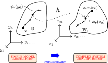
Figure 3: The conjugation, $h$, maps orbits $\psi_{\tau}(u_{0})$, with initial condition (point at $\blacksquare$) $y_{0}$ in the parameter space $\mathbb{U}$, to orbits $\phi_{\tau}(x_{0})$ on $\mathbb{W}_{s}$, corresponding to the initial condition $x_{0}=h(u_{0})$.

Given the orbit, $\psi_{\tau}(y_{0})$, on $\mathbb{U}$, with initial condition $\psi_{0}(y_{0})=y_{0}$, the conjugate flow, $\phi_{\tau}(x_{0})$, will correspond to the orbit with initial condition $\phi_{0}(x_{0})=x_{0}=h(y_{0})$ on $\mathbb{W}_{s}$ and we can write eq. 6 as

$$h\circ\psi_{\tau}(y_{0})=\phi_{\tau}(x_{0})$$ (7)

which shows that $h$ maps orbits in $\mathbb{U}$ onto orbits in $\mathbb{W}_{s}$ while keeping the time parametrization. Figure 3 gives a schematic illustration of the topics discussed here. Consider an invariant-set $Q$ in $\mathbb{U}$ i.e. $\psi_{\tau}(Q)\subset Q$ for all $\tau$. From the conjugation relation eq. 7 it then follows that $\phi_{\tau}(h(Q))=\phi_{\tau}(S)=h\circ\psi_{\tau}(Q)\subset h(Q)=S$, where $S=h(Q)$, and

$$\psi_{\tau}(Q)\subset Q\Leftrightarrow\phi_{\tau}(S)\subset S$$ (8)

where the left arrow follows from considering the inverse transformation $h^{-1}$ (i.e. the map from $\mathbb{W}_{s}$ to $\mathbb{U}$). An invariant set, under $\psi_{\tau}$ on $\mathbb{U}$, $Q$, thus corresponds to an invariant set, $S=h(Q)$, under the conjugated flow, $\phi_{\tau}$, on $\mathbb{W}_{s}$; and vice-versa. Repeating this analysis for the iterated map version of eq. 6 it follows that invariant sets under the iterated map are also preserved. The oscillator limit-cycles $\xi,\gamma$, are invariant sets of the flows $\psi_{\tau},\phi_{\tau}$ on $\mathbb{U}$ and $\mathbb{W}_{s}$, respectively, and from eq. 8

$$h(\xi)=\gamma$$ (9)

Likewise, the leaves,of the isochrone foliation on $\mathbb{U}(\xi)$ are an invariant of $2\pi$-iterated map, $\psi_{2\pi}$.

4.2 Choosing a specific NF-OSC template model : the PNF-OSC

Figure 4: Transient orbits, and limit-cycle $\xi$, of the PNF-OSC system defined in eq. 10. The example system considered here is $5$-dimensional with $m=1,k=1$ ($1$ additional real + $1$ complex mode) described in-terms of coordinates $\bar{y}=(r,\phi,w_{1},z_{1},z_{2})\in\mathbb{R}^{5}$ where $w_{1}=y_{3}$, $z_{1}=y_{4}$ and $z_{2}=y_{5}$ (see text). Parameters are fixed as $(\mu,\beta_{1},\sigma_{1},\nu_{1})=(0.5,0.2,0.1,0,3)$. Two cross sections are shown where $(y_{1},y_{2},w_{1}=y_{3})$ (red curve) shows the effects of the additional real mode whereas $(y_{1},y_{2},z_{1}=y_{4})$ (blue curve) which shows the effects of the complex mode.

We consider the $n$-dimensional parameter manifold $\mathbb{U}$ indexed by the Cartesian coordinate set $y=(y_{1},y_{2},\cdots,y_{n})\in\mathbb{R}^{n}$ (see section 4 and fig. 3). Let $r=\sqrt{y_{1}^{2}+y_{2}^{2}}$, $\phi=\arctan(y_{2}/y_{1})$ be the polar coordinates indexing the $y_{1},y_{2}$ plane and consider the transformed coordinates $\bar{y}=(\phi,r,w,z)\in\mathbb{R}^{n}$ where sub-coordinate vectors $w\in\mathbb{R}^{m}$ and $z\in\mathbb{R}^{2k}$ contain the remaining $n{-}2$ $y$-coordinates. As $\bar{y}$ is an $n$-dimensional coordinate system the dimension of these sub-vectors are constrained through $n=2+m+2k$ (see footnote 8). As $n\geq 2$ is assumed, it always possible to find two numbers $m,k\geq 0$ such that this constraint is upheld.

Proposition 4.1.

The new coordinates $\bar{y}=(\phi,r,w,z)\in\mathbb{R}^{n}$, indexing the parameter manifold $\mathbb{U}$, are orthogonal.

Proof.

The polar coordinates $(\phi,r)$, indexing the $y_{1},y_{2}$ plane, represent an orthogonal coordinate system in this plane [29]. The remaining coordinates $(y_{3},\cdots,y_{n})\in\mathbb{R}^{n-2}$ are orthogonal to the $y_{1},y_{2}$ plane and furthermore comprised of Cartesian coordinate functions; which are of-course, by definition, orthogonal. However, coordinate sub-vectors $w,z$ are simply containers holding this remaining set of Cartesian $y$-coordinates (see text above and footnote 8) and it hence follows trivially that $\bar{y}=(\phi,r,w,z)=(\phi,r,y_{3},y_{4},\cdots y_{n})\in\mathbb{R}^{n}$ is an orthogonal coordinate system. ∎

In these new coordinates, the dynamics of the NF-OSC on $\mathbb{U}$, is modelled in-terms of the autonomous ODE, $\dot{y}=g(y)$, of the form

$$\dot{\phi}=1$$ (10)

$$\dot{r}=\mu r(1-r)$$

$$\dot{w}_{i}=-\beta_{i}w_{i}\quad i=1,2,\cdots,m$$

$$\dot{z}_{2i-1}=-\sigma_{i}z_{2i-1}+\nu_{i}z_{2i}\quad i=1,2,\cdots,k$$

$$\dot{z}_{2i}=-\sigma_{i}z_{2i}-\nu_{i}z_{2i-1}\quad i=1,2,\cdots,k$$

with $\mu,\alpha,\beta_{i},\sigma\in\mathbb{R}^{+}$ are a collection of positive real parameters whereas $\nu_{i}\in\mathbb{R}\backslash\{0\}$ is a non-zero real parameter. From inspection, it follows that the system in eq. 10 generates a single stable limit-cycle set

$$\xi=\bigl{\{}\bar{y}\in\mathbb{U}\,\,:\,\,(\phi,r,\{w,z\})=[0;2\pi)\times 1\times\{\bm{0}\}\bigr{\}}$$ (11)

with $\{\bm{0}\}=0\times 0\times 0\times\cdots\times 0$ (m+2k times) and eq. 11 hence simply describes a unit circle in the $y_{1},y_{2}$ plane. Henceforth, the NF-OSC, $\mathbf{o}=(\psi_{\tau},\xi)$, where $\psi_{\tau}$ is the flow on $\mathbb{U}$ generated by integrating the ODE in eq. 10, will be known as the PNF-OSC (polar normal-form).

Proposition 4.2.

the PNF-OSC system, defined in-terms of the ODE in eq. 10, belong to the OFD oscillator class, $\mathbf{o}\in\mathbf{O}^{\perp}$.

Proof.

From eq. 2 the bundle $\mathsf{T}_{\gamma}\mathbb{R}^{n}$ is spanned by the Floquet vectors $(u_{1}(\tau),u_{2}(\tau),\cdots,u_{n}(\tau))$. From eq. 23 in appendix A we have $\mathsf{T}_{\xi}\mathbb{R}^{n}=\text{span}(\hat{\phi},\hat{r},\{\hat{w}_{i}\}_{i=1}^{m},\{\hat{z}_{2i}\pm j\hat{z}_{2i-1}\}_{i=1}^{k})$ with the notation, $\hat{x}$, representing the coordinate-vector corresponding to coordinate function, $x$. From proposition 4.1 the coordinate system $\bar{y}=(\phi,r,w,z)$ is orthogonal which implies that the corresponding coordinate vectors $\hat{\phi},\hat{r},\hat{w}_{i}$ etc. are orthogonal. By definition (see eq. 3) $\mathsf{T}_{\xi}\mathbb{R}^{n}\in\mathbf{B}^{\perp}$ and from the definition in eq. 4 we get $\mathbf{o}\in\mathbf{O}^{\perp}$. ∎

The dynamics corresponding to the $w$ and $z$ coordinate sets generate $m$ real and $k$ imaginary stable Floquet modes. The orbits of an example 5-dimensional PNF-OSC system ($m=k=1$) were calculated by numerically integrating eq. 10 and the resulting curves are plotted in fig. 4 together with the limit-cycle, $\xi$, defined in eq. 11.

Figure 5: (a) The PNF-OSC oscillator $\mathbf{o}=(\psi_{\tau},\xi)\in\mathbf{O}^{\perp}$ with stable (parametrization) manifold $\mathbb{U}$. (b) the unspecified N-OSC oscillator $\mathbf{q}=(\phi_{\tau},\gamma)$ with stable manifold $\mathbb{W}_{s}$. The PNF-OSC provides a parametrization of the N-OSC in $\mathbb{W}_{s}$ in-terms of the conjugation map $h$. This parametrization is faithful, mapping the limit-cycle in $\mathbb{U}$, $\xi$, onto the corresponding limit-cycle in $\mathbb{W}_{s}$, $\gamma$, and the individual isochrone foliation leaves (purple curves) in $\mathbb{U}$ onto the corresponding sets in $\mathbb{W}_{s}$ (see discussion in section 3.1).

4.3 The set $\mathbf{H}_{C}$ and operator $\overset{c}{\sim}_{h}$

We seek to use parametrization, $\mathbf{o}\sim\mathbf{q}$, in-order to identify all N-OSC oscillators $\mathbf{q}=(\phi_{\tau},\gamma)$ on $\mathbb{W}_{s}$ which belong to the class $\mathbf{O}^{\perp}$. From proposition 4.2, $\mathbf{o}\in\mathbf{O}^{\perp}$, and this in-turn places certain limitations on $h\bigl{|}_{\xi}$ ($h$ restricted to $\xi$)

Proposition 4.3.

Let $\mathbf{o}\sim_{h}\mathbf{q}$ where $\mathbf{o}=(\psi_{\tau},\xi)\in\mathbf{O}^{\perp}$ is the PNF-OSC defined in eqs. 10 and 11. Then $\mathbf{q}\in\mathbf{O}^{\perp}\Leftrightarrow h\bigl{|}_{\xi}\text{is conformal (angle preserving)}$.

Proof.

From eq. 5 it follows that at every point of the PNF-OSC PSS orbit $y_{s}(\tau)\in\xi$, the Jacobian $dh$ maps tangent-spaces in $\mathbb{T}_{\xi}\mathbb{R}^{n}$ onto tangent-spaces $\mathbb{T}_{\gamma}\mathbb{R}^{n}$ of the conjugated orbit $x_{s}(\tau)\in\gamma$. From proposition 4.2, $\mathbb{T}_{\xi}\mathbb{R}^{n}\in\mathbf{B}^{\perp}$, and tangent-spaces along $\xi$ are all spanned by orthogonal basis-vectors. The N-OSC tangent-bundle (see section 3.2) will be orthogonal, $\mathbb{T}_{\gamma}\mathbb{R}^{n}\in\mathbf{B}^{\perp}$, if, and only if, the Jacobian is angle-preserving (conformal) at all points of $\xi$. This implies that $dh(y_{s}(\tau))\in\text{CO}(n)$ must hold for all $\tau$ where we let $\text{CO}(n)$ be the set of all $n\times n$ conformal matrices. By definition, $h\bigl{|}_{\xi}$ is then conformal. ∎

Let $\mathbf{H}$ be the set of all conjugation maps. The subset $\mathbf{H}_{\text{C}}\subset\mathbf{H}$, and the conjugation operator $\overset{c}{\sim}$, are then defined as

$$\mathbf{H}_{\text{C}} =\{h\in\mathbf{H}:h\bigl{|}_{\xi}\text{is conformal}\}$$ (12)

$$\overset{c}{\sim}_{h} :=\,\sim_{h}\,\,\wedge\,\,h\in\mathbf{H}_{\text{C}}$$

and $\overset{c}{\sim}$ is simply $\sim$ with the extra condition that the conjugation map, $h$, belongs to $\mathbf{H}_{\text{C}}$ (conformal restriction). It can be shown that $\overset{c}{\sim}$ is an equivalence operator. We can then re-state proposition 4.3

Proposition 4.4 (proposition 4.3 re-stated).

Let $\mathbf{o}\in\mathbf{O}^{\perp}$ be the PNF-OSC on $\mathbb{U}$. Then $\mathbf{q}\in\mathbf{O}^{\perp}\Leftrightarrow\mathbf{o}\overset{c}{\sim}\mathbf{q}$.

Proof.

Follows directly from proposition 4.3 and the definitions in eq. 12. ∎

Let us briefly explain this result. Assuming the PNF-OSC, $\mathbf{o}=(\psi_{\tau},\xi)$, on $\mathbb{U}$, is used as a parametrization template. Proposition 4.4 then says that, in-order for $\mathbf{q}=(\phi_{\tau},\gamma)$ on $\mathbb{W}_{s}$ to be an OFD oscillator, there must exist a conjugation map $h$, with a conformal restriction on $\xi$ (i.e. $h\in\mathbf{H}_{\text{C}}$) such that $\mathbf{o}\overset{c}{\sim}_{h}\mathbf{q}$ (and not just the standard $\mathbf{o}\sim_{h}\mathbf{q}$).

5 Main result : OFD and PSS symmetry correlation

The conjugation relation eq. 6 is valid at every point of domains $\mathbb{U}$ and $\mathbb{W}_{s}$, respectively. This, by definition, then implies that it also holds on all open sets contained in these spaces[27, 28]. We consider the following open neighborhoods $\Gamma_{\xi}=\{y\in\mathbb{U},\epsilon\in\mathbb{R}^{+}:\|y-\xi\|\leq\epsilon\}\subset\mathbb{U}$ and $\Gamma_{\gamma}=\{x\in\mathbb{W}_{s},\varepsilon\in\mathbb{R}^{+}:\|x-\gamma\|\leq\varepsilon\}\subset\mathbb{W}_{s}$ which describe tubular open sets enclosing the limit-cycles $\xi,\gamma$.

Proposition 5.1.

Consider the (local) conjugation map $h:\Gamma_{\xi}\to\Gamma_{\gamma}$. If $h\in\mathbf{H}_{C}$, with $\mathbf{H}_{C}\subset\mathbf{H}$ defined in eq. 12, then this map must have the following representation on $\Gamma_{\xi}$

$$h(y)=\nu(y)+H(y)$$ (13)

where $\nu:\Gamma_{\xi}\to\Gamma_{\gamma}$ is a conformal map which restricts to $h$ on $\xi$, $h(\xi)\equiv h\bigl{|}_{\xi}=\nu\bigl{|}_{\xi}\equiv\nu(\xi)$ and where $H:\Gamma_{\xi}\to\Gamma_{\gamma}$ is some unspecified map with $H(\xi)=0$.

Proof.

For every conformal restriction, $h\bigl{|}_{\xi}$, at-least one conformal map, $\nu:\Gamma_{\xi}\to\Gamma_{\gamma}$, must exist; i.e. simply continue the power-series expansion of the restriction $h\bigl{|}_{\xi}$, around $\xi$, in every possible way that keeps $\nu$ conformal. Let $H=h-\nu$ denote the residual. By definition this residual is non-conformal on $\xi$ since all conformal contributions are contained in $\nu$. It then follows directly that $H(\xi)=0$. ∎

The following statement discuss the possible forms the conformal map $\nu$, in proposition 5.1, can take

Proposition 5.2.

Any conformal conjugation map $\nu:\Gamma_{\xi}\to\Gamma_{\gamma}$, must have the form

$$\nu(y)=\rho Ay$$ (14)

where $\rho\in\mathbb{R}\setminus\{0\}$ is a non-zero real value and $A\in O(n)$ is an orthogonal matrix.

Proof.

For $n>2$ this is a direct consequence of Liouville’s theorem (1850) [19, 20, 21, 22, 23]. This theorem states that all conformal maps on an open region of $\mathbb{R}^{n}$, with $n>2$, must be Möbius transformations of the form $\nu(y)=b+\rho A(y-a)/|y-a|^{s}$, with $a,b\in\mathbb{R}^{n}$, $\rho\in\mathbb{R}$, $A\in O(n)$ and the integer exponent $s$ is either $0$ or $2$. We first consider the case $s=2$. This map will have a singularity at $y=a$. From the discussion in section 4.1, the conjugation-map transform orbits into orbits (see eq. 7). This singularity would hence imply that orbits around $y=a$ would be mapped to orbits around infinity; clearly not a possibility. Hence we must have $s=0$ which implies a map $\nu(y)=d+\rho Ay$ where $d=b-\rho Aa$ is a real parameter. Both oscillators are assumed to have fixed-points at the origin (see sections 3 and 4 and footnotes 6 and 10) and we hence must have $\nu(0)=0$ which implies $d=0$ and we reached eq. 14. For the special planar case, $n=2$, $\nu$ is a bi-holomorphic map on the annuli $\Gamma_{\xi}$. Schottkys Theorem (1877)[18] states that the map must have the form $k(z)=az^{\pm 1}$ where $a\in\mathbb{C}\setminus\{0\}$. Again, since singularities are not allowed and we must have $k(0)=0$ this implies the map $k(z)=az$. Equation 14 is then reached by transforming from complex to real coordinates in the plane. ∎

At this point we define the set of rotational symmetric curves centered at the origin and with radius $r$, on $\mathbb{W}_{s}$

$$\mathcal{SYM}_{n}=\bigl{\{}x\in\mathbb{R}^{n},\exists r\in\mathbb{R}^{+}\,\,:\,\,\lVert x\rVert-r=0\bigr{\}}$$ (15)

From eq. 11, the PNF-OSC limit-cycle belongs to this set, $\xi\in\mathcal{SYM}_{n}$. This fact allow us to state the main result of this paper

Theorem 5.1.

Let $\mathbf{q}=(\phi_{\tau},\gamma)\in\mathbf{O}$ be any given oscillator on $\mathbb{W}_{s}$. Then

$$\mathbf{q}\in\mathbf{O}^{\perp}\Rightarrow\gamma\in\mathcal{SYM}_{n}$$ (16)

Proof.

From proposition 4.4 we must have $\mathbf{o}\overset{c}{\sim}\mathbf{q}$ where $\mathbf{o}=(\psi_{\tau},\xi)$ is the PNF-OSC described in section 4.2. This implies that the conjugation map, $h$, must belong to the set, $\mathbf{H}_{\text{C}}$, defined in eq. 12. From proposition 5.1, this implies a conjugation map of the form $h(y)=\nu(y)+H(y)$ with $h(\xi)=\nu(\xi)$. Proposition 5.2 and eq. 9 then yield $\gamma=h(\xi)=\nu(\xi)=\rho Ay$ , with $y\in\xi$. This describes a linear rotation + scaling of $\xi$ which implies $\xi\in\mathcal{SYM}_{n}\Rightarrow\gamma=h(\xi)\in\mathcal{SYM}_{n}$, as linear rotation + scaling preserves symmetry of $\xi\in\mathcal{SYM}_{n}$ (i.e. maps $\mathcal{SYM}_{n}$ into $\mathcal{SYM}_{n}$). ∎

Firstly, it is important to note that the result in theorem 5.1 represents a one-way implication. In other words, the OFD property implies PSS symmetry. No reverse relation exists as discussed, at length, in the introduction; i.e. symmetry does not imply an OFD. Secondly, the result, implicitly, also hold for symmetric limits-sets on $\mathbb{W}_{s}$ with center away from the origin even-though $\mathcal{SYM}_{n}$ in eq. 15 seem to include this restriction. Theorem 5.1 explains why OFD’s generally are not observed in real-life oscillator systems where non-linear device-models make it impossible to attain perfect PSS symmetry. The methodology developed in the previous sections, leading to the main result in theorem 5.1, is given the SYM-OFD calling handle; signifying the (one-way) relation between PSS symmetry and LR OFD described in theorem 5.1.

5.1 Discussion of the result in theorem 5.1

It may seem that the result in theorem 5.1 is of limited scope since it relies on the specific choice of the PNF-OSC normal-form model. Luckily, because $\overset{c}{\sim}$ is an equivalence relation (see eq. 12 and footnote 9), this turns out not to be an issue. Assume we had chosen some other OFD NF-OSC model, call it XNF-OSC, $\mathbf{x}=(\theta_{\tau},\sigma)\in\mathbf{O}^{\perp}$ with stable manifold $\mathbb{X}=\mathbb{R}^{n}\backslash\{0\}$. Since the PNF-OSC is an OFD oscillator, $\mathbf{o}\in\mathbf{O}^{\perp}$, it follows from proposition 4.4 that a map, $k:\mathbb{U}\to\mathbb{X}\in\mathbf{H}_{C}$, must exist such that $\psi_{\tau}\overset{c}{\sim}_{k}\theta_{\tau}$. Equivalently, if the N-OSC $\mathbf{q}=(\phi_{\tau},\gamma)$ is an OFD oscillator, $\theta_{\tau}\overset{c}{\sim}_{f}\phi_{\tau}$. Since $\overset{c}{\sim}$ is an equivalence relation (see eq. 12 and footnotes 9 and 7) it follows from transitivity

$$\psi_{\tau}\overset{c}{\sim}_{k}\theta_{\tau}\wedge\theta_{\tau}\overset{c}{\sim}_{f}\phi_{\tau}\Rightarrow\psi_{\tau}\overset{c}{\sim}_{h}\phi_{\tau}$$ (17)

where $h$ is the composition $h=k\circ f\equiv k(f)$. The statement in theorem 5.1 is hence independent of the choice of normal-form (NF-OSC) and hence unique. Or said another way : eq. 17 shows that the XNF-OSC, $\mathbf{x}$, and the PNF-OSC, $\mathbf{o}$, give the same OFD classification of the N-OSC, $\mathbf{q}$.

The range of an equivalence relation, i.e. the types of oscillators which can be parameterized, is limited by the topological invariants. Each set of invariant values defines a unique equivalence class which is preserved under conjugation [27, 28]. The invariants do not change under conjugation and it follows that a oscillators in one equivalence class (defined in-terms of one sets of invariants) cannot parameterize a system in a different class; as this would correspond to a different set of invariants. For hyperbolic oscillators, on identical domains $\mathbb{U}=\mathbb{W}_{s}$, the only invariant of importance is the M-MATRIX stability measure characterized in-terms of the NF-OSC M-MATRIX eigenvalue-spectrum, $\text{spec}\{\Psi\}$. From proposition 4.2 and appendix A, the PNF-OSC was specifically designed such that all possible M-MATRIX eigenvalue-spectra can be modelled, i.e any combination of $\{\lambda_{i}\}_{i=1}^{n}$, inside the unit-circle on the complex plane ($|\lambda_{i}|\leq 1$ for stable oscillators), and this model is hence able to parameterize all oscillators on $\mathbb{W}_{s}$.

The results derived herein are thus fully independent of the specific choice NF-OSC model. The PNF-OSC model was only chosen in-order to facilitate the analysis leading to theorem 5.1. We could easily have chosen any other equivalent model and would have arrived at the exact same result. The equivalence topics discussed herein are well-known concepts developed within the field of topological conjugation theory; a mature and established branch of modern dynamical systems theory. The SYM-OFD model, and specifically theorem 5.1, is hence based on an extremely rigorous foundation of theoretical research which stretches back several decades [27, 28, 29, 33, 34, 35, 30, 31, 32, 19, 20, 21, 22, 23, 18].

6 Numerical experiments

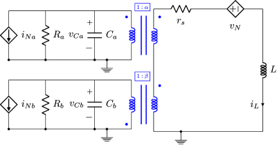
(a) TCR-OSC

(b) FET-OSC

Figure 6: (a) : transformer coupled resonator oscillator (TCR-OSC), $(i_{Na},i_{Nb})$ are trans-conductors (nonlinear conductors) and $v_{N}$ is a trans-impedance (nonlinear resistor). (b) MOSFET oscillator (MOS-OSC) oscillator with both parallel (blue) and series (red) resonator resistor options.

The transformers in the TCR-OSC circuit, shown in fig. 6.(a), are perfectly ideal with turn-ratios $\alpha,\beta$ and with the lower transformer inducing a $180^{\circ}$ phase shift. Time-normalization, $\tau=t\omega_{0}$, is introduced with $\omega_{0}=1.0/\sqrt{LC_{s}}$ and $C_{s}=C_{a}C_{b}/(C_{a}+C_{b})$. The time-normalized equations of the TCR-OSC circuit are then written

$$\sigma_{a}\dot{y} =-y/Q_{a}+\alpha_{n}v/z_{0}+i_{Na}(y,v,w)$$ (18)

$$\dot{v} =-v/Q_{s}+z_{0}(\alpha y-\beta w)+v_{N}(y,v,w)$$

$$\sigma_{b}\dot{w} =-w/Q_{b}+\beta_{n}v/z_{0}+i_{Nb}(y,v,w)$$

where $x=(y,v,w)=(v_{Ca}/z_{0},i_{L}z_{0},v_{Cb}/z_{0})\in\mathbb{R}^{3}$ is the normalized $3$-D circuit state-vector with $z_{0}=\sqrt{L/C_{s}}$ and $\sigma_{a,b}=C_{a,b}/C_{s}$, $\alpha_{n}=\alpha/(\alpha^{2}+\beta^{2})$, $\beta_{n}=\beta/(\alpha^{2}+\beta^{2})$, $Q_{a,b}=\omega_{0}C_{a}R_{a,b}$, $Q_{s}=\omega_{0}L/r_{s}$. The trans-conductors and trans-impedance controlled sources (negative conductors/resistors) are defined in-terms of the functions $i_{N(a|b)}(x)=(\alpha_{n}|\beta_{n})z_{0}[\alpha y-\beta w]f(x)$ and $v_{N}(x)=(v/z_{0})f(x)$ with $f:\mathbb{R}^{3}\to\mathbb{R}$ being the real function $f(x)=\bigl{(}p-\bigl{(}q_{1}[\alpha z_{0}y-\beta z_{0}w]^{2}+q_{2}(v/z_{0})^{2}\bigr{)}$. These types of polynomial functions, discussed here, are readily implemented electrically using e.g. standard operational amplifiers (op-amp) circuits, operational trans-conductance amplifiers (OTA) or dedicated chips. We will not dwell on this practical implementation issue here as this topic is not critical for the discussion below. Unless stated otherwise the circuit parameters are fixed as $\alpha=\beta=1/\sqrt{2}$, $C_{a}=C_{b}\Rightarrow\sigma_{a}=\sigma_{b}=2$, $z_{0}=1\Omega$, $Q_{a}=Q_{b}=Q_{s}=100$, $p=0.06\mathrm{A/V}$ , $q_{1}=0.003\mathrm{A/V^{2}}$, $q_{2}=0.003\mathrm{A^{-1}}$, $s=1\mathrm{V/A}$.

The FET-OSC circuit in fig. 6.(b) is a differential pair FET LC oscillator configuration. The circuit includes both an option for parallel (blue) and series (red) resonator resistance topology. In the simulations below the FET differential-pair circuit is modelled in-terms of the trans-conductance function $\Theta(\zeta)=I_{B}(2/\pi)\arctan([\pi/2](G_{m}/I_{B})\zeta)$ which has been demonstrated to be a excellent approximation of the actual device model[36]. Here $\zeta$ represents the input voltage across the pair and $G_{m}=\sqrt{k_{n}I_{B}}$ is the small-signal trans-conductance where $k_{n}=\mu_{n}C_{\text{ox}}W_{n}/L_{n}$ with $\mu_{n},C_{\text{ox}},W_{n}$ and $L_{n}$ are the charge mobility, oxide capacitance, gate width and length, respectively. The normalized time-variable is given as, $\tau=t\omega_{0}$, where $\omega_{0}=1.0/\sqrt{L_{p}C_{s}}$, $C_{s}=C_{1}C_{2}/(C_{1}+C_{2})$ and $L_{p}=L_{1}L_{2}/(L_{1}+L_{2})$. The time-normalized dynamic equations, of the circuit in fig. 6.(b), are then written

$$\sigma_{1}\dot{q} =-{\color[rgb]{0,0,1}q/Q_{p1}}-r/z_{0}+\Theta(z_{0}[q-s])$$ (19)

$$\kappa_{1}\dot{r} =z_{0}q-{\color[rgb]{1,0,0}r/Q_{s1}}$$

$$\sigma_{2}\dot{s} =-{\color[rgb]{0,0,1}s/Q_{p2}}-u/z_{0}-\Theta(z_{0}[q-s])$$

$$\kappa_{2}\dot{u} =z_{0}s-{\color[rgb]{1,0,0}u/Q_{s2}}$$

where $x=(q,r,s,u)=(v_{C1}/z_{0},i_{L1}z_{0},v_{C2}/z_{0},i_{L2}z_{0})\in\mathbb{R}^{4}$ is the (normalized) $4$-D state vector with $z_{0}=\sqrt{L_{p}/C_{s}}$. The blue/red contributions in eq. 19 correspond to the blue/red parts of the FET-OSC circuit in fig. 6.(b), $Q_{p1,2}=\omega_{0}C_{1,2}r_{p1,2}$, $Q_{s1,2}=\omega_{0}L_{1,2}/r_{s1,2}$, $\sigma_{1,2}=C_{1,2}/C_{s}$ and $\kappa_{1,2}=L_{1,2}/L_{p}$. Unless otherwise stated the parameters are fixed as $Q_{p1,2}=Q_{s1,2}=100$, $C_{1}=C_{2}\Rightarrow\sigma_{1,2}=2.0$, $L_{1}=L_{2}\Rightarrow\kappa_{1,2}=2.0$, $I_{B}=8\mathrm{mA}$ and $k_{n}=2\mathrm{AV^{-2}}$ (time-scaled value).

6.1 The simulation measures

The N-OSC limit-cycle on $\mathbb{W}_{s}$ is written componentwise as $\gamma(\tau)=(\gamma_{1}(\tau),\gamma_{2}(\tau),\cdots,\gamma_{n}(\tau))$ where $\gamma(\tau)=\gamma(\tau+2\pi)$ (due to time-normalization, see section 3). Given the $2\pi$ periodic function $\rho(\tau)=\sum_{i=1}^{n}\gamma_{i}^{2}(\tau)$ the following two measures are introduced

$$\Lambda =\Biggl{|}\frac{1}{2\pi}\int_{0}^{2\pi}\biggl{\{}(\rho(\tau)/\rho_{\max})-1.0\biggr{\}}d\tau\biggr{|}$$ (20)

$$\Upsilon =\underset{i,j\in[1;n]}{\max}\bigl{\{}\Theta_{ij}\bigr{\}}\,,\,\text{with}$$

$$\Theta_{ij} =\underset{\tau\in[0;2\pi]}{\max}\bigl{|}|\angle\{u_{i}(\tau),u_{j}(\tau)\}|-\pi/2\bigr{|}$$

where $\rho_{\max}$ represents the maximal value of the function $\rho$ on the interval $\tau\in[0;2\pi)$ and $u_{i}(\tau)$ is the $i$th Floquet mode. From inspection it should be clear that $\Lambda$ in measures the closeness of the limit-cycle $\gamma$ on $\mathbb{W}_{s}$ to members of the set $\mathcal{SYM}_{n}$ in eq. 15 whereas $\Upsilon$ measures the closeness of a N-OSC solution, $\mathbf{q}\in\mathbf{O}$, to a member of the special OFD oscillator class $\mathbf{O}^{\perp}$ defined in eq. 4.

Remark 6.1.

From eq. 20 and footnote 13, in-order for the result in theorem 5.1 to be valid the relations $\Upsilon\rightarrow 0\Rightarrow\Lambda\rightarrow 0$ must be observed in all numerical experiments. This is of-course equivalent to $\Upsilon\rightarrow-\infty\Rightarrow\Lambda\rightarrow-\infty$ on the dB scale; i.e. $10\log_{10}(\Lambda),10\log_{10}(\Upsilon)$.

The predictions made in remark 6.1 are now tested in fig. 7 on a simple van-der-Pol oscillator. From the insets in this figure, the PSS is seen to approach an elliptical limit-set as $\epsilon\to 0$ for all values of $c_{0}$ except for the value $c_{0}=1$. The exception, $c_{0}=1.0$, approaches a rotational symmetric set $\gamma\in\mathcal{SYM}_{2}$ (see eq. 15). From remark 6.1, we need to see that $\Upsilon\rightarrow 0$, implies, $c_{0}=1$; exactly because $\Lambda\rightarrow 0$, as $\epsilon\to 0$, only for $c_{0}=1$. Inspecting fig. 7 this is indeed the case.

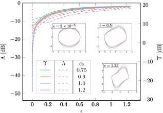
Figure 7: Simulations for the simple van-der-Pol oscillator, $\dot{x}=c_{0}y$, $\dot{y}=-x+\epsilon(1.0-x^{2})y$. The two measures $\Lambda$ and $\Upsilon$, defined in (20), are plotted in the logarithmic dB scale $10\log_{10}(\Lambda),10\log_{10}(\Upsilon)$) and insets of the oscillator limit-cycles, at various parameter points (color-codes match those in $\Upsilon,\Gamma$-tables), are included.

6.2 Simulation results

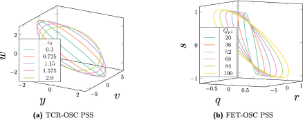
Figure 8: (a) : TCR-OSC PSS (see eq. 18, fig. 6.(a)) $z_{0}:0.3\to 2.0$. (b) : FET-OSC PSS (see eq. 19, fig. 6.(b)) parallel resonator (blue), $Q_{p1}:20\to 100$.

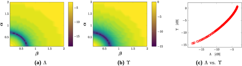
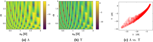
Figure 9: Simulations for the TCR-OSC circuit in eqs. 18 and 6.(a). (a)-(b) : 2D sweep of measures $\Upsilon$ and $\Lambda$ in dB (i.e. $10\log_{10}(\Lambda),10\log_{10}(\Upsilon)$) defined in eq. 20, (c) : a scatter plot of the points in (a) ($10\log_{10}(\Lambda)$) vs. the points in (b) ($10\log_{10}(\Upsilon)$). Upper row : sweep of parameters $\alpha,\beta\in[0.1;2.0]\times[0.1;2.0]$. Lower row : sweep of parameters $\alpha,z_{0}\in[0.1;2.0]\times[0.3;2.0]$.

Figure 8 plots the PSS orbits (limit-cycles) corresponding to the oscillator circuits in fig. 6. The figures illustrate how the PSS symmetry can be increased/descreased by varying the circuit parameters defined in connection with eqs. 18 and 19. Once the PSS has been calculated, the measure, $\Lambda$, is readily calculated from eq. 20. Based on this PSS, the Floquet modes $\{u_{i}(\tau),v_{i}(\tau),\mu_{i}\}$ are derived by integrating the LR equations corresponding to this solution[1, 2, 4] (see also section 3.2) and the measure, $\Upsilon$, follows from eq. 20.

Considering the TRC-OSC circuit in fig. 6.(a), the two measures are calculated, as explained above, while sweeping circuit parameters $(z_{0},\alpha,\beta)$. Figure 9 (upper row) depicts contour plots for the two measures $\Lambda,\Upsilon$ as functions of turn-ratios $\alpha,\beta$ swept in the interval $[0.1;2.0]\times[0.1;2.0]$. Inspecting these two images one immediate observation is that the pattern of the contours appear very similar. This suspicion is then directly confirmed in fig. 9.(c) which plots the points in these two figures against each other as a scatter-plot format. It is strikingly clear from this plot that the measures are very strongly correlated. The figure furthermore reveals the relationship $\Upsilon\to 0\Rightarrow\Lambda\to 0$ ($-\infty$ on dB scale) and from remark 6.1 this observation therefore directly serves to validate the novel SYM-OFD model derived herein. In the lower row of fig. 9 these same simulations are repeated but this time $\alpha,z_{0}$ are swept in the range $[0.1;2.0]\times[0.3;5.0]$. The figure again shows the measures obeying the predictions laid out in remark 6.1 and hence again serve to validate the model. Finally, fig. 10 shows two equivalent simulation sweeps for the FET-OSC circuit in fig. 6.(b) with both figures serving to validate the novel SYM-OFD model developed herein.

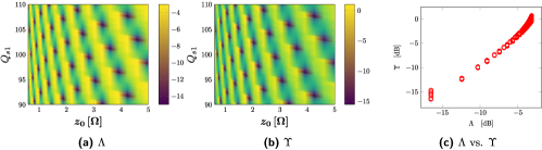
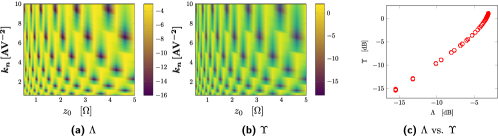
Figure 10: Simulations for the FET-OSC circuit in eqs. 19 and 6.(b). Figure content/symbols as in fig. 9. Upper row : sweep of parameters $(Q_{s1},z_{0})\in[90;110]\times[0.6;5.0]$. Lower row : sweep of parameters $z_{0},k_{n}\in[0.6;5]\times[0.5;10.0]$.

6.3 Summary of Simulation Results

The 13 simulations in figs. 7, 9 and 10, divided into 3 figures, all together serve to validate the SYM-OFD model developed herein. By varying the circuit parameters we can control both the symmetry properties of the steady-state (see fig. 8) and the Floquet decomposition of the LR (level of orthogonality). Inspecting, fig. 7 and the 2-D contour plots + scatter plots in figs. 9 and 10 it is clear that these two properties are closely correlated, i.e. orthogonality increases $\Rightarrow$ symmetry increases; as was first predicted in theorem 5.1.

It is important to note that this idea is completely novel. There is absolutely nothing in the definition of symmetry/orthogonality measures $\Lambda,\Upsilon$ in eq. 20 that reveals that these should be related in any way or form. Hence, the observation described in remark 6.1 is completely unanticipated. It cannot be reached by arguments based on empirical or phenomenological reasoning but relies on the rigorous formulation developed herein.

7 Conclusion

We prove that in order to achieve an orthogonal Floquet decomposition of the oscillator linear-response, which implies zero AM-PM noise conversion, an oscillator must produce a rotationally symmetric steady-state solution. This novel link connecting the configuration of a Floquet decomposition with symmetry properties of the underlying steady-state is a novel concept which, to our knowledge, is first discussed here for the general case. Our results can be interpreted as a condition for the leaves of the oscillator isochrone foliation to intersect the limit-cycle set orthogonally. We performed a series of numerical experiments on higher dimensional oscillators with all simulations unequivocally supporting the predictions of the proposed model.

Appendix A The PNF-OSC Floquet decomposition

The Jacobian matrix $J_{\xi}\in\mathbb{R}^{n\times n}$ is now calculated as the derivative of the ODE in eq. 10 at every point on $\xi$ in eq. 11. Due to the perfect symmetry of these equations it follows easily that this matrix is constant (independent of coordinates) and has the block-diagonal form $J_{\xi}=\text{diag}(0,-2\mu,W,Z)$ where $W\in\mathbb{R}^{m\times m}$ is the $m$-dimensional constant diagonal matrix $W=\text{diag}(-\beta_{1},-\beta_{2},\cdots,-\beta_{m})$ whereas $Z\in\mathbb{R}^{2k\times 2k}$ is the constant $2k$-dimensional block diagonal matrix $Z=\text{diag}(Z_{1},Z_{2},\cdots,Z_{k})$ with $Z_{i}=\bigl{[}\begin{smallmatrix}-\sigma_{i}&\nu_{i}\\ -\nu_{i}&-\sigma_{i}\end{smallmatrix}\bigr{]}$. Note that $W,Z$ are the sub-Jacobian matrices corresponding to the $w,z$ equations in eq. 10. The PNF-OSC F-MATRIX map $\Psi(t,s)$ (see discussion section 3.2) is then calculated as the solution to the Jacobian equation $\dot{\Psi}(t,s)=J_{\xi}\Psi(t,s)$. Given that $J_{\xi}$ is constant, and block-diagonal, a closed form solution is easily derived. The PNF-OSC Monodromy (M-MATRIX) $\Psi_{2\pi}$ is then found from this F-MATRIX solution as $\Psi_{2\pi}=\Psi(2\pi+s,s)$. Following this recipe the PNF-OSC M-MATRIX is derived as

$$\Psi_{2\pi} =\text{diag}(1,-2\mu\pi,W_{2\pi},Z_{2\pi})$$ (21)

$$W_{2\pi} =\text{diag}(\exp(-2\beta_{1}\pi),\exp(-2\beta_{2}\pi),\cdots,\exp(-2\beta_{m}\pi))$$

$$Z_{2\pi} =\text{diag}(P\Lambda_{1}P^{-1},P\Lambda_{2}P^{-1},\cdots,P\Lambda_{k}P^{-1})$$

where $\Lambda_{i}=\text{diag}(\exp(2\pi[-\sigma_{i}+j\nu_{i}]),\exp(2\pi[-\sigma_{i}-j\nu_{i}])$ and $P=\frac{1}{\sqrt{2}}\bigl{[}\begin{smallmatrix}j&-j\\ 1&1\end{smallmatrix}\bigr{]}$. Let $\text{EIGV}(\Psi_{2\pi})$ be the collection of M-MATRIX eigenvectors. It then follows from inspection of eq. 21 that

$$\text{EIGV}(\Psi_{2\pi})=\bigl{[}\hat{\phi},\hat{r},\{\hat{w}_{i}\}_{i=1}^{m},\{\hat{z}_{2i}\pm j\hat{z}_{2i-1}\}_{i=1}^{k}\bigr{]}$$ (22)

where $\hat{\phi},\hat{r},\hat{w}_{i}$ etc. represents the coordinate vectors corresponding to coordinates $\bar{y}=(\phi,r,w,z)$ (see text in section 4.2 and footnote 8). The PNF-OSC Floquet decomposition $(u_{1}(s),u_{2}(s),\cdots,u_{n}(s))$, at phase $\phi=s$, simply correspond to the eigenvectors for the M-MATRIX (which are independent of $s$ due to symmetry).

$$(u_{1}(\tau),u_{2}(\tau),\cdots,u_{n}(\tau))=(\hat{\phi},\hat{r},\{\hat{w}_{i}\}_{i=1}^{m},\{\hat{z}_{2i}\pm j\hat{z}_{2i-1}\}_{i=1}^{k})$$ (23)

where, following the notation introduced in section 3.2 we let $\tau\in[0,2\pi)$ index the phase of the Floquet vectors (instead of $\phi$). The M-MATRIX eigenvalue-spectrum, also know as the characteristic multiplies $\{\lambda_{i}\}_{i=1}^{n}$, follow straight from inspection of eq. 21

$$\begin{gathered}\textnormal{spec}\{\Psi_{2\pi}\}=\{\lambda_{i}\}_{i=1}^{n}=\bigl{[}1,\exp(-\mu 2\pi),\{\exp(-2\pi\beta_{i})\}_{i=1}^{m},\\ \{\exp(-2\pi|\sigma_{i}|\pm j2\pi\nu_{i})\}_{i=1}^{k}\bigr{]}\end{gathered}$$ (24)

The PNF-OSC in eq. 10 is hence able to generate any possible M-MATRIX eigenvalue-spectrum (real modes + complex modes) by simply varying the discrete parameters $m,k$ and the value of circuit parameters $\{\mu,\beta_{i},\sigma_{i},\nu_{i}\}$.

Acronyms

LR

linear-response.

F-MATRIX

fundamental matrix map.

M-MATRIX

Monodromy matrix (special F-MATRIX).

PSS

periodic steady-state.

SYM-OFD

handle for the model developed herein.

N-OSC

$n$-dimensional hyperbolic stable oscillator.

NF-OSC

normal-form oscillator.

PNF-OSC

polar normal-form oscillator.

OFD

orthogonal Floquet decomposition.

Symbols

$\mathbf{o}$

the (P)NF-OSC, $\mathbf{o}=(\psi_{\tau},\xi)$.

$\mathbf{q}$

the N-OSC, $\mathbf{q}=(\phi_{\tau},\gamma)$.

$\psi_{\tau},\phi_{\tau}$

(P)NF/N-OSC flow maps.

$\xi,\gamma$

(P)NF/N-OSC hyperbolic limit-cycles.

$\mathbb{U},\mathbb{W}_{s}$

(P)NF/N-OSC stable manifolds (domains).

$\mathbf{B}$

the set of all oscillator tangent bundles.

$\mathbf{B}^{\perp}$

OFD tangent bundles (subset of $\mathbf{B}$).

$\mathbf{O}$

the set of all hyperbolic stable oscillators.

$\mathbf{O}^{\perp}$

set of OFD oscillators, i.e. circuits with OFD tangent bundles, $\mathbf{B}^{\perp}$, (subset of $\mathbf{O}$).

$\mathbf{H}$

set of smooth conjugation maps $h:\mathbb{U}\to\mathbb{W}_{s}$.

$\mathbf{H}_{C}$

$h\in\mathbf{H}_{C}\subset\mathbf{H}$ if $h\bigl{|}_{\xi}$ (restriction to $\xi$) is conformal (angle preserving).

$\mathcal{SYM}_{n}$

the set of all perfectly symmetric $n$-dimensional limit-cycles (closed curves).

$\sim_{h}$

the conjugation operator (equivalence relation) in-terms of the unique conjugation map $h$.

$\mathbf{o}\sim_{h}\mathbf{q}$

conjugate oscillators $\mathbf{o}$ and $\mathbf{q}$.

$\overset{c}{\sim}_{h}$

the $\sim_{h}$ operator + restriction $h\in\mathbf{H}_{C}$.

References

- [1] F. X. Kärtner, “Analysis of white and f- noise in oscillators,” International Journal of Circuit Theory and Applications, vol. 18, no. 5, pp. 485–519, 1990.
- [2] A. Demir, A. Mehrotra, and J. Roychowdhury, “Phase noise in oscillators: A unifying theory and numerical methods for characterization,” IEEE Transactions on Circuits and Systems I: Fundamental Theory and Applications, vol. 47, no. 5, pp. 655–674, 2000.
- [3] G. J. Coram, “A simple 2-d oscillator to determine the correct decomposition of perturbations into amplitude and phase noise,” IEEE Transactions on Circuits and Systems I: Fundamental Theory and Applications, vol. 48, no. 7, pp. 896–898, 2001.
- [4] T. Djurhuus, V. Krozer, J. Vidkjær, and T. K. Johansen, “Oscillator phase noise: A geometrical approach,” IEEE Transactions on Circuits and Systems I: Regular Papers, vol. 56, no. 7, pp. 1373–1382, 2009.
- [5] B. Razavi, “A study of phase noise in cmos oscillators,” IEEE journal of Solid-State circuits, vol. 31, no. 3, pp. 331–343, 1996.
- [6] C. Samori, A. L. Lacaita, F. Villa, and F. Zappa, “Spectrum folding and phase noise in lc tuned oscillators,” IEEE Transactions on Circuits and Systems II: Analog and Digital Signal Processing, vol. 45, no. 7, pp. 781–790, 1998.
- [7] A. Laloue, J.-C. Nallatamby, M. Prigent, M. Camiade, and J. Obregon, “An efficient method for nonlinear distortion calculation of the am and pm noise spectra of fmcw radar transmitters,” IEEE transactions on Microwave Theory and Techniques, vol. 51, no. 8, pp. 1966–1976, 2003.
- [8] H.-C. Chang, X. Cao, U. K. Mishra, and R. A. York, “Phase noise in coupled oscillators: Theory and experiment,” IEEE Transactions on Microwave Theory and Techniques, vol. 45, no. 5, pp. 604–615, 1997.
- [9] M. Bonnin, F. Corinto, and M. Gilli, “Phase space decomposition for phase noise and synchronization analysis of planar nonlinear oscillators,” IEEE Transactions on Circuits and Systems II: Express Briefs, vol. 59, no. 10, pp. 638–642, 2012.
- [10] M. Bonnin and F. Corinto, “Influence of noise on the phase and amplitude of second-order oscillators,” IEEE Transactions on Circuits and Systems II: Express Briefs, vol. 61, no. 3, pp. 158–162, 2014.
- [11] F. L. Traversa and F. Bonani, “Oscillator noise: A nonlinear perturbative theory including orbital fluctuations and phase-orbital correlation,” IEEE Transactions on Circuits and Systems I: Regular Papers, vol. 58, no. 10, pp. 2485–2497, 2011.
- [12] T. Djurhuus, V. Krozer, J. Vidkjar, and T. K. Johansen, “Trade-off between phase-noise and signal quadrature in unilaterally coupled oscillators,” in IEEE MTT-S International Microwave Symposium Digest, 2005. IEEE, 2005, pp. 4–pp.
- [13] T. Djurhuus, V. Krozer, J. Vidkjær, and T. K. Johansen, “Nonlinear analysis of a cross-coupled quadrature harmonic oscillator,” IEEE Transactions on Circuits and Systems I: Regular Papers, vol. 52, no. 11, pp. 2276–2285, 2005.
- [14] ——, “Am to pm noise conversion in a cross-coupled quadrature harmonic oscillator,” International Journal of RF and Microwave Computer-Aided Engineering, vol. 16, no. 1, pp. 34–41, 2006.
- [15] T. Djurhuus and V. Krozer, “A study of amplitude-to-phase noise conversion in planar oscillators,” International Journal of Circuit Theory and Applications, vol. 49, no. 1, pp. 1–17, 2021.
- [16] F. X. Kaertner, “Determination of the correlation spectrum of oscillators with low noise,” IEEE Transactions on Microwave Theory and Techniques, vol. 37, no. 1, pp. 90–101, 1989.
- [17] M. Galassi, J. Davies, J. Theiler, B. Gough, G. Jungman, P. Alken, M. Booth, F. Rossi, and R. Ulerich, GNU scientific library. Network Theory Limited, 2002.
- [18] K. Astala, T. Iwaniec, G. Martin, and J. Onninen, “Schottkys theorem on conformal mappings between annuli: A play of derivatives and integrals,” Contemporary Mathematics, vol. 455, pp. 35–39, 2008.
- [19] P. Hartman, “Systems of total differential equations and liouville’s theorem on conformal mappings,” American Journal of Mathematics, vol. 69, no. 2, pp. 327–332, 1947.
- [20] H. FLANDERS, “Liouville’s theorem on conformal mapping,” Journal of Mathematics and Mechanics, vol. 15, no. 1, pp. 157–161, 1966.
- [21] H. Jacobowitz et al., “Two notes on conformal geometry,” Hokkaido Mathematical Journal, vol. 20, no. 2, pp. 313–329, 1991.
- [22] W. Kühnel and H.-B. Rademacher, “Liouville’s theorem in conformal geometry,” Journal de mathématiques pures et appliquées, vol. 88, no. 3, pp. 251–260, 2007.
- [23] T. Iwaniec and G. Martin, “The liouville theorem,” in Analysis And Topology: A Volume Dedicated to the Memory of S Stoilow. World Scientific, 1998, pp. 339–361.
- [24] A. T. Winfree, “Biological rhythms and the behavior of populations of coupled oscillators,” Journal of theoretical biology, vol. 16, no. 1, pp. 15–42, 1967.
- [25] J. Guckenheimer, “Isochrons and phaseless sets,” Journal of Mathematical Biology, vol. 1, no. 3, pp. 259–273, 1975.
- [26] S. Srivastava and J. Roychowdhury, “Analytical equations for nonlinear phase errors and jitter in ring oscillators,” IEEE Transactions on Circuits and Systems I: Regular Papers, vol. 54, no. 10, pp. 2321–2329, 2007.
- [27] S. Wiggins, S. Wiggins, and M. Golubitsky, Introduction to applied nonlinear dynamical systems and chaos. Springer, 1990, vol. 2.
- [28] Y. A. Kuznetsov, Elements of applied bifurcation theory. Springer Science & Business Media, 2013, vol. 112.
- [29] T. Frankel, The geometry of physics: an introduction. Cambridge university press, 2011.
- [30] X. Cabré, E. Fontich, and R. de la Llave, “The parameterization method for invariant manifolds i: manifolds associated to non-resonant subspaces,” Indiana University mathematics journal, pp. 283–328, 2003.
- [31] ——, “The parameterization method for invariant manifolds i: manifolds associated to non-resonant subspaces,” Indiana University mathematics journal, pp. 283–328, 2003.
- [32] X. Cabré, E. Fontich, and R. De La Llave, “The parameterization method for invariant manifolds iii: overview and applications,” Journal of Differential Equations, vol. 218, no. 2, pp. 444–515, 2005.
- [33] G. Huguet and R. d. l. Llave, “Computation of limit cycles and their isochrones: fast algorithms and their convergence,” 2012.
- [34] G. Huguet and R. de la Llave, “Computation of limit cycles and their isochrons: fast algorithms and their convergence,” SIAM Journal on Applied Dynamical Systems, vol. 12, no. 4, pp. 1763–1802, 2013.
- [35] G. Huguet, A. Pérez-Cervera et al., “A geometric approach to phase response curves and its numerical computation through the parameterization method,” arXiv preprint arXiv:1809.07318, 2018.
- [36] F. Pepe and P. Andreani, “Still more on the phase noise performance of harmonic oscillators,” IEEE Transactions on Circuits and Systems II: Express Briefs, vol. 63, no. 6, pp. 538–542, 2016.