A Genuine Multipartite Entanglement Measure Generated by the Parametrized Entanglement Measure

Abstract

In this paper, we investigate a genuine multipartite entanglement measure based on the geometric method. This measure arrives at the maximal value for the absolutely maximally entangled states and has desirable properties for quantifying the genuine multipartite entanglement. We present a lower bound of the genuine multipartite entanglement measure. At last, we present some examples to show that the genuine entanglement measure is with distinct entanglement ordering from other measures, and we also present the advantages of the measure proposed here with other measures.

I introduction

Quantum entanglement is an essential feature of quantum mechanics. It plays an important role in quantum information and quantum computation theory horodecki2009quantum , such as superdense coding bennett1992communication , teleportation bennett1993teleporting and the speedup of quantum algorithms shimoni2005entangled .
One of the most important problems is to quantify the entanglement in a composite quantum system. Vedral $et$ $al.$ in vedral1997quantifying presented the condition that the amount of entanglement cannot increase under local operation and classical communication (LOCC) is necessary for an entanglement measure. Then Vidal considered the entanglement measures with stronger properties and proposed a general mathematical framework to build entanglement monotone with functions satisfying some properties for pure statesvidal2000entanglement . The other interesting approach with operational significance to quantify the entanglement is proposed in gour2020optimal ; shi2021extension . Compared with the bipartite entanglement systems, the complexity of a multipartite entanglement system grows remarkly with the increasing number of parties and the increasing dimension of the systems. The notion of multipartite entanglement measure can be refined into the so-called genuine multipartite entanglement (GME) guhne2005multipartite ; plenio2014introduction . Substantial results have been achiveved on the GME measures in the last few decades meyer2002global ; blasone2008hierarchies ; hiesmayr2009two ; ma2011measure ; jungnitsch2011taming ; rafsanjani2012genuinely ; xie2021triangle ; beckey2021computable ; guo2022genuine ; li2022geometric . In blasone2008hierarchies , the authors proposed a genuinely entangled measure defined as the shortest distance from a given state to the k-separable states, which was denoted as generalized geometric measure (GGM). The other GME measure, the genuinely multipatite concurrence (GMC) was defined as the minimal bipartite concurrence among all bipartitions ma2011measure . However, the above two measures cannot show all the conditions of entanglement among the parties, both two are defined on the minimizations of the partitions. Concurrence fill was proposed as a three-qubit GME measure xie2021triangle , it is the square of the area of the three-qubit concurrence triangle. The authors in guo2022genuine generalized the above method to build a multipartite entanglement measure, however, it is hard when the parties are bigger. Hence there is much work to do on how to understand and quantify the multipartite entanglement. Recently, another method to investigate the GME measure is proposed, it was based on the geometric mean of all bipartite entanglement measure concurrence li2022geometric .
In this paper, we investigate a GME measure which was based on the geometric mean in terms of a bipartite entanglement measure, $F_{q}$ yang2021parametrized . This measure satisfies the following properties, subadditivity, continuity for pure states. We also present the bound of this GME measure based on the method proposed in dai2020experimentally . At last, we present some examples to show that the GME measure proposed here is with different orders from GMC and GGM, we also prsent some advantages of the measure when comparing with GMC and GGM.
This paper is organised as follows. In Sec. II, we present the preliminary knowledge needed here. In Sec. III, we present the main results. We show that the measure is a GME measure, then we consider the measure for the W states and GHZ states in $n$-qubit systems and present that the GHZ states is more entangled than the W states. We also present the measure satifies the subadditivity and continuity for pure states. And then we present a lower bound of the measure for multipartite mixed states. We also make some comparisons between the measure proposed here and the GMC, GGM by considering some examples. In Sec. IV, we end with a conclusion.

II Preliminary Knowledge

Concurrence is one of the most important entanglement measures for bipartite quantum systems hill1997entanglement , it has attracted much attention of the relevant researchers since the end of the last century wootters1998entanglement ; coffman2000distributed ; mintert2004concurrence ; chen2005concurrence ; zhang2016evaluation ; dai2020experimentally ; li2020improved . For a bipartite pure state $|\psi\rangle_{AB},$ its concurrence is defined as

$$C(|\psi\rangle_{AB})=\sqrt{2(1-Tr_{A}|\psi\rangle\langle\psi|)},$$ (1)

when $\rho_{AB}$ is a mixed state, its concurrence is defined as

$$C(\rho_{AB})=\mathop{\rm min}\sum_{i}p_{i}C(|\psi\rangle_{i}),$$ (2)

where the minimum takes over all the decompositions of $\rho_{AB}=\sum_{i}p_{i}|\psi_{i}\rangle\langle\psi_{i}|.$ For two qubit mixed states, there exists a direct link between the concurrence and the entanglement of formation wootters1998entanglement .

As a generalized von Neumann entropy, Tsallis-$q$ entropy tsallis1988possible ; landsberg1998distributions can present more properties of the entangled states tsallis2001peres ; rossignoli2002generalized . For a pure state $|\psi\rangle_{AB}=\sum_{i}\sqrt{\lambda_{i}}|ii\rangle,$ then its Tsallis-$q$ entanglement measure san2010tsallis is defined as

$$T_{q}(|\psi\rangle_{AB})=\frac{1-\rho_{A}^{q}}{q-1},$$

here $\rho_{A}=Tr_{B}\rho_{AB},$ $q\in(0,1)\cup(1,\infty).$

Motived by the Tsallis-$q$ entanglement entropy, Yang $et$ $al.$ proposed a parametrized entanglement measure, $q$-concurrence, for a bipartite entanglement systems yang2021parametrized . When $|\psi\rangle_{AB}$ is a pure state, this measure is defined as

$$\mathcal{C}_{q}(|\psi\rangle_{AB})=F_{q}(\rho_{A}),$$ (3)

here $F(\rho)=1-\mathop{\rm Tr}\rho^{q}$, $q\geq 2.$ When $\rho_{AB}$ is a mixed state, its $q$-concurrence is defined as

$$\mathcal{C}_{q}(\rho_{AB})=\mathop{\rm min}\sum_{i}p_{i}\mathcal{C}_{q}(|\psi_{i}\rangle),$$ (4)

where the minimum takes over all the decompositions of $\rho_{AB}=\sum_{i}p_{i}|\psi_{i}\rangle\langle\psi_{i}|.$

Next we recall some properties of the function $F_{q}(\rho)$ proposed in yang2021parametrized .

Lemma 1

For any density matrix $\rho$ and $q\geq 2$, $F_{q}(\rho)$ satisfies the following properties:

• Non-negativity: $F_{q}(\rho)\geq 0.$

• Subadditivity: For a general bipartite state $\rho_{AB}$, $F_{q}(\rho_{AB})$ satisfies the inequalies:

  $$|F_{q}(\rho_{A})-F_{q}(\rho_{B})|\leq F_{q}(\rho_{AB})\leq F_{q}(\rho_{A})+F_{q}(\rho_{B}).$$ (5)

• Concavity

  $$\sum p_{i}F_{q}(\rho_{i})\leq F_{q}(\sum_{i}p_{i}\rho_{i}),$$ (6)

  where $p_{i}\in(0,1],$ and $\sum_{i}p_{i}=1$, $\rho_{i}$ are density matrices. Furthermore, The equality holds if and only if $\rho_{i}$ are identical for all $p_{i}>0.$

• quasiconvex:

  $$F_{q}(\sum_{i}p_{i}\rho_{i})\leq\sum p_{i}^{q}F_{q}(\rho_{i})+1-\sum_{i}p_{i}^{q},$$ (7)

  where the inequality holds if and only if $\rho_{i}=|\psi_{i}\rangle\langle\psi_{i}|,$ and $\{|\psi_{i}\rangle\}$ are orthogonal.

Due to the properties of $F_{q}(\rho)$ above, we have that the maximum of $F_{q}(|\psi\rangle_{AB})$ is attained when its reduced density matrix of the smaller subsystem is the maximally mixed state, that is,

$$\mathop{\rm max}_{|\psi\rangle_{AB}}F_{q}(|\psi\rangle_{AB})=\frac{d^{q-1}-1}{d^{q-1}},$$

here $d$ is the dimension of the smaller system.

Next we review the knowledge needed on multipartite entanglement.

An $n$-partite pure state $|\psi\rangle_{A_{1}A_{2}\cdots A_{n}}$ is full product if it can be written as

$$|\psi\rangle_{A_{1}A_{2}\cdots A_{n}}=|\phi_{1}\rangle_{A_{1}}|\phi_{2}\rangle_{A_{2}}\cdots|\phi_{n}\rangle_{A_{n}},$$ (8)

otherwise, it is entangled. A multipartite pure state is called genuinely entangled if

$$|\psi\rangle_{A_{1}A_{2}\cdots A_{n}}\neq|\phi\rangle_{S}|\zeta\rangle_{\overline{S}},$$ (9)

for any partite $S|\overline{S}$, here $S$ is a subset of $\boldsymbol{A}=\{A_{1},A_{2},\cdots,A_{n}\}$, and $\overline{S}=\boldsymbol{A}-S$. An $n$ partite mixed state $\rho$ is biseparable if it can be written as a convex combination of biseparable pure states $\rho=\sum_{i}p_{i}|\psi_{i}\rangle\langle\psi_{i}|,$ where the pure states in $\{|\psi_{i}\rangle\}$ can be biseparable with respect to some bipartitions. If an $n$-partite state is not biseparable, then it is genuinely entangled.

Then we recall the necessary conditions of a genuine multipartite entanglement (GME) measure $E$ should satisfy ma2011measure :

• . it is entanglement monotone.

• . $E(\rho)=0,$ if $\rho$ is biseparable.

• . $E(\rho)>0$, if $\rho$ is genuinely entangled state.

Based on the $q$-concurrence, we present a GME measure in terms of the geometric methods.

Definition 2

Assume $|\psi\rangle_{A_{1}A_{2}\cdots A_{n}}$ is an $n$-partite pure state, the geometric mean of $q$-concurrence $(GqC)$ is defined as

$$\mathcal{G}_{q}(|\psi\rangle)=[\mathcal{P}_{q}(|\psi\rangle)]^{\frac{1}{c(\alpha)}},$$ (10)

where $\alpha=\{\alpha_{i}\}$ is the set that denotes all possible bipartitions $\{A_{\alpha_{i}}|B_{\alpha_{i}}\}$ of the $n$ parties, $c(\alpha)$ is the cardinality of $\alpha$, and $\mathcal{P}_{q}(|\psi\rangle)$ is

$$\mathcal{P}_{q}(|\psi\rangle)=\Pi_{\alpha_{i}\in\alpha}{\mathcal{C}_{q}}_{A_{\alpha_{i}}B_{\alpha_{i}}}(|\psi\rangle),$$

$$\begin{split}c(\alpha)=\left\{\begin{array}[]{lr}\sum_{m=1}^{\frac{n-1}{2}}C_{n}^{m},\hskip 8.53581pt\textit{if $n$ is odd,}\\ \sum_{m=1}^{\frac{n-2}{2}}C_{n}^{m}+\frac{1}{2}C_{n}^{\frac{n}{2}},\hskip 8.53581pt\textit{if $n$ is even.}\end{array}\right.\end{split}$$

When $\rho$ is an $n$-partite mixed state,

$$\mathcal{G}_{q}(\rho)=\mathop{\rm min}\sum_{i}p_{i}\mathcal{G}_{q}(|\psi_{i}\rangle),$$ (11)

where the minimum takes over all the decompositions of $\rho=\sum_{i}p_{i}|\psi_{i}\rangle\langle\psi_{i}|.$

III MAIN RESULTS

In this section, we present the main results of this article. In Sec. III.1, we present the properties of the GqC. In Sec. III.2, a lower bound of the GqC for an $n$-partite mixed state $\rho$ was presented. In Sec. III.3, we make a comparison of the GqC with other GME measures.

III.1 The properties of GqC

Here we first show that the GqC is a GME measure.

Theorem 3

For an arbitrary $n$-partite quantum state $|\psi\rangle_{A_{1}A_{2}\cdots A_{n}}$, the GqC is a GME measure.

Proof.

Here we show that the GqC satisfies the properties $2$ and $3$. The proof of the property 1 is similar to the proof in li2022geometric , and we omit it here.

Assume $|\psi\rangle$ is a biseparable pure state, then according to the definition of biseparable states in Sec. II, there exists a partition $S|\overline{S}$ of $\boldsymbol{A}$ such tat $|\psi\rangle=|\phi_{1}\rangle_{S}|\phi_{2}\rangle_{\overline{S}}$, $\mathcal{C}_{q}(|\psi\rangle_{S|\overline{S}})=0$, thus we have $\mathcal{G}_{q}(|\psi\rangle)=0.$ And due to the definition of the GqC for mixed states, when a mixed state $\rho$ is biseparable, $\mathcal{G}_{q}(\rho)=0,$ Hence we present the proof of condition 1.

As a GME pure state $|\psi\rangle$ can be written as (9), that is, $|\psi\rangle$ cannot be written as product states with respect to any bipartition, then we have all the bipartite $\mathcal{C}_{q}$ is bigger than 0, so $\mathcal{G}_{q}(|\psi\rangle)>0.$ And due to the definition of a mixed GME state $\rho$ and the definition of GqC, we have when $\rho$ is GME, $\mathcal{G}_{q}(\rho>0),$ then we prove the condition $2.$     $\sqcap$$\sqcup$

A pure multipartite entangled state is called absolutely maximally entangled state (AMES) if all reduced density operators obtained by tracing out at least half of the particles of the pure state are maximally mixed helwig2012absolute . The AMES can be used to develop the quantum secret sharing shemes helwig2013absolutely and quantum error correction codes grassl2015quantum ; alsina2021absolutely . And the GHZ state is the only AMES up to the local unitary operations in three qubit systems goyeneche2015absolutely ; shi2021multilinear . Due to the definitions and properties of $\mathcal{C}_{q}(|\psi\rangle)$, when $|\psi\rangle$ is an AMES, then $\mathcal{G}_{q}(\cdot)$ gets the maximum, that is, it can also be seen as a proper GME measure li2022geometric .
Next we consider two pure states in multipartite systems that are inequivalent in terms of stochastic LOCC (SLOCC), the W states and GHZ states. The authors in joo2003quantum showed that in three qubit systems, a perfect teleportation can be performed via the GHZ state, while the W state cannot. Moreover, for a $k$-partite W and GHZ state ($k\geq 3$), the infimum asymptotic ratio from GHZ to W is 1, however, the infimum asymptotic ratio from W to GHZ is bigger than 1 vrana2015asymptotic . Thus the GHZ states can be thought more entangled than the W states.

Example 4

$$|W_{n}\rangle= \frac{1}{\sqrt{n}}(|10\cdots 0\rangle+|01\cdots 0\rangle+\cdots+|00\cdots 1\rangle),$$

$$|GHZ_{n}\rangle= \frac{1}{\sqrt{2}}(|00\cdots 0\rangle+|11\cdots 1\rangle),$$

Here we place the results on $\mathcal{G}_{q}(|W_{n}\rangle)$ and $\mathcal{G}_{q}(|GHZ_{n}\rangle)$ in Sec. V.1. In Fig. 1, we can see the values of $\frac{\mathcal{G}_{3}(|W_{n}\rangle)}{\mathcal{G}_{3}(|GHZ_{n}\rangle)}$ tends to 1 with the increase of $n$.

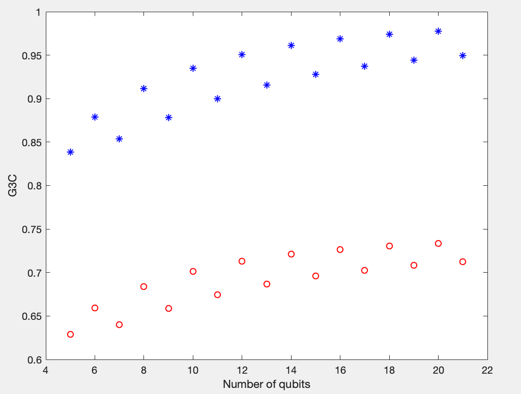
Figure 1: In this figure, we plot the $\mathcal{G}_{3}(|W_{n}\rangle)$ with the red circle and $\frac{\mathcal{G}_{3}(|W_{n}\rangle)}{\mathcal{G}_{3}(|GHZ_{n}\rangle)}$ with the star when $n$ from $5$ to 21.

Next we show the GqC satisfies the subadditivity and continuity for pure states. First we prove the subadditivity.

Assume $|\psi_{1}\rangle$ and $|\psi_{2}\rangle$ are pure states in a bipartite system $\mathcal{H}_{d_{1}}\otimes\mathcal{H}_{d_{2}},$ then we have

$$\mathcal{C}_{q}(|\psi_{1}\rangle\otimes|\psi_{2}\rangle)-\mathcal{C}_{q}(|\psi_{1}\rangle)-\mathcal{C}_{q}(|\psi_{2}\rangle)$$

$$=1-\mathop{\rm Tr}\rho_{A}^{q}\mathop{\rm Tr}\sigma_{A}^{q}-1+\mathop{\rm Tr}\rho_{A}^{q}-1+\mathop{\rm Tr}\sigma_{A}^{q}$$

$$=-(1-\mathop{\rm Tr}\rho_{A}^{q})(1-\mathop{\rm Tr}\sigma_{A}^{q})\leq 0,$$

here we denote $\rho_{A}=tr_{B}|\psi_{1}\rangle_{AB}\langle\psi_{1}|,$ $\sigma_{A}=tr_{B}|\psi_{2}\rangle_{AB}\langle\psi_{2}|$. Due to the above inequality, we have $\mathcal{C}_{q}(\cdot)$ is subadditivity for pure states in arbitrary dimensional bipartite systems.

$$\mathcal{C}_{q}(|\psi_{1}\rangle\otimes|\psi_{2}\rangle)\leq\mathcal{C}_{q}(|\psi_{1}\rangle)+\mathcal{C}_{q}(|\psi_{2}\rangle).$$ (12)

Then we show that $\mathcal{G}_{q}(\cdot)$ satisfies the subadditivity property for pure states.

Assume $|\psi_{1}\rangle$ and $|\psi_{2}\rangle$ are two pure states in $n$-partite systems, then we have

$$(\mathcal{G}_{q}(|\psi_{1}\rangle\otimes|\psi_{2}\rangle)^{c(\alpha)}-(\mathcal{G}_{q}(|\psi_{1}\rangle)+\mathcal{G}_{q}(|\psi_{2}\rangle))^{c(\alpha)}$$

$$= \Pi_{\alpha_{i}\in\alpha}\mathcal{C}_{qA_{\alpha_{i}}B_{\alpha_{i}}}(|\psi_{1}\rangle\otimes|\psi_{2}\rangle)-[(\Pi_{\alpha_{i}\in\alpha}\mathcal{C}_{qA_{\alpha_{i}}B_{\alpha_{i}}}(|\psi_{1}\rangle))^{\frac{1}{c(\alpha)}}+(\Pi_{\alpha_{i}\in\alpha}\mathcal{C}_{qA_{\alpha_{i}}B_{\alpha_{i}}}(|\psi_{2}\rangle))^{\frac{1}{c(\alpha)}}]^{c(\alpha)}$$

$$\leq \Pi_{\alpha_{i}\in\alpha}(\mathcal{C}_{qA_{\alpha_{i}}B_{\alpha_{i}}}(|\psi_{1}\rangle)+\mathcal{C}_{qA_{\alpha_{i}}B_{\alpha_{i}}}(|\psi_{2}\rangle))-[(\Pi_{\alpha_{i}\in\alpha}\mathcal{C}_{qA_{\alpha_{i}}B_{\alpha_{i}}}(|\psi_{1}\rangle))^{\frac{1}{c(\alpha)}}+(\Pi_{\alpha_{i}\in\alpha}\mathcal{C}_{qA_{\alpha_{i}}B_{\alpha_{i}}}(|\psi_{2}\rangle))^{\frac{1}{c(\alpha)}}]^{c(\alpha)}$$

$$\leq 0,$$ (13)

here the first inequality is due to the subadditivity of the bipartite entanglement measure $(\ref{sub}),$ the second inequality is due to the Mahler’s inequality. Due to the inequality (13), we have $\mathcal{G}_{q}(\cdot)$ satisfies the subadditivity for pure states.

At last, we present that the GqC satisfies continuity for pure states. First we present a lemma on the $\mathcal{C}_{q}(\cdot)$ of pure states.

Lemma 5

Assume $|\psi_{1}\rangle$ and $|\psi_{2}\rangle$ are pure states in $\mathcal{H}_{d}\otimes\mathcal{H}_{d},$ when $\lVert|\psi_{1}\rangle-|\psi_{2}\rangle\rVert_{1}\leq\epsilon$, then we have

$$|\mathcal{C}_{q}(|\psi_{1}\rangle)-\mathcal{C}_{q}(|\psi_{2}\rangle)|\leq d[(1+\frac{\epsilon}{d})^{q}-1].$$ (14)

Then we can generalize the results to the GqC for the pure states.

Theorem 6

Assume $|\psi_{1}\rangle$ and $|\psi_{2}\rangle$ are two pure states in $n$-partite systems $\mathcal{H}_{d}\otimes\mathcal{H}_{d}\otimes\cdots\otimes\mathcal{H}_{d}$, here $\lVert|\psi_{1}\rangle-|\psi_{2}\rangle\rVert\leq\epsilon,$ then we have

$$|\mathcal{G}_{q}(|\psi_{1}\rangle)-\mathcal{G}_{q}(|\psi_{2}\rangle)|\leq[\sum_{i=1}^{\frac{n-1}{2}}C_{n}^{i}d^{i}[(1+\frac{\epsilon}{d^{i}})^{q}-1]]^{\frac{1}{c(\alpha)}}$$ (15)

Here we place the proof of the lemma 5 and Theorem 6 in Sec. V.2.

III.2 A lower bound of GqC

In this subsection, we first present a lower bound of the entanglement measure $\mathcal{C}_{q}(\rho_{AB})$ for a bipartite mixed state $\rho_{AB}$, then we extend the results to the GqC for multipartite mixed states.

Theorem 7

For a bipartite mixed state $\rho$ on the system $\mathcal{H}_{m}\otimes\mathcal{H}_{n}(m\leq n)$, $|\phi\rangle$ is an arbitrary pure state in $\mathcal{H}_{m}\otimes\mathcal{H}_{n}$ its revised parametrized entanglement measure $\mathcal{C}_{q}(\rho)$ satisfies

$$\mathcal{C}_{q}(\rho)\geq{co[R(\Lambda)]},$$ (16)

where $\Lambda=\mathop{\rm max}\{\frac{\langle\phi|\rho|\phi\rangle}{s_{1}m},\frac{1}{m}\}$, $R(\Lambda)=1-\gamma(\Lambda)^{q}-\frac{[1-\gamma(\Lambda)]^{q}}{(m-1)^{q-1}},$ with $\gamma(\Lambda)=\frac{\sqrt{\Lambda}+\sqrt{(m-1)(1-\Lambda)}}{m}$, and

$$co[R(\Lambda)]=\frac{m^{q-1}-1}{m^{q-2}(m-1)}(\Lambda-\frac{1}{m}).$$

We place the proof of this theorem in the Appendix V.3.

Before generalizing the bound for $\mathcal{C}_{q}(\rho_{AB})$ of a bipartite state $\rho_{AB}$ to $\mathcal{G}_{q}(\rho_{A_{1}A_{2}\cdots A_{n}})$ of a multipartite mixed state $\rho_{A_{1}A_{2}\cdots A_{n}}$, we will denote some definitions. Let $|\psi\rangle_{A_{1}A_{2}\cdots A_{n}}$ be an arbitrary $n$-partite pure state in $\mathcal{H}_{A_{1}}\otimes\mathcal{H}_{A_{2}}\otimes\cdots\otimes\mathcal{H}_{A_{n}},$ $\alpha_{i}$ be a possible bipartition of $\{A_{1},A_{2},\cdots,A_{n}\},$ then by the Schmidt decomposition, $|\psi\rangle_{A_{1}A_{2}\cdots A_{n}}$ can be written as $|\psi\rangle=U_{\alpha}\otimes U_{\overline{\alpha}}\sum_{i=1}^{q_{\alpha}}\sqrt{s_{i}^{(\alpha)}}|ii\rangle$ under the bipartition $\alpha|\overline{\alpha},$ here $\{\sqrt{s_{i}^{(\alpha)}}\}$ are the Schmidt coefficients in decreasing order, $m_{\alpha}$ denotes the number of nonzero Schmidt coefficients. Next let $s_{1}=\mathop{\rm max}_{\alpha}\{s_{1}^{\alpha}\},$ $m=\mathop{\rm max}_{\alpha}\{m_{\alpha}\}.$

Theorem 8

Assume $\rho_{A_{1}A_{2}\cdots A_{n}}$ is a mixed state on an $n$-paritite system. Then we have

$$\mathcal{G}_{q}(\rho)\geq\frac{m^{q-1}-1}{m^{q-2}(m-1)}(\Lambda^{{}^{\prime}}-\frac{1}{m}),$$ (17)

here we denote $\Lambda^{{}^{\prime}}=\mathop{\rm max}\{\frac{\langle\phi|\rho|\phi\rangle}{s_{1}m},\frac{1}{m}\}$

We place the proof of Theorem 8 in the Sec. V.4. Next we present an example to show the results.

Example 9

Consider a $3$-qubit $W$ state with the white noise,

$$\rho_{W}=p|W\rangle\langle W|+\frac{1-p}{8}\mathbb{I},\hskip 8.53581ptp\in(0,1).$$ (18)

here we present the bound of $\mathcal{G}_{2}(\cdot)$ for $\rho_{W}$ in Fig. 2. There we plot the lower bound of G$2$C for $\rho_{W}$.

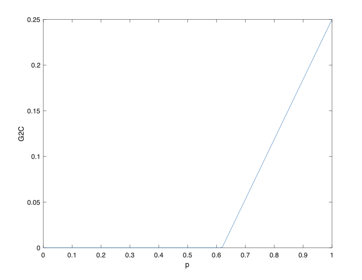
Figure 2: In this figure, the red line denotes the lower bound of G2C for $\rho_{W}$, here we use $|\phi\rangle=|W\rangle$ and $s_{1}=\frac{2}{3}.$

Example 10

Let $\rho_{GHZ}$ be a $3$-qubit mixed state,

$$\rho_{GHZ}= c|GHZ\rangle\langle GHZ|+\frac{1-c}{8}\mathbb{I},$$

$$|GHZ\rangle= \frac{1}{\sqrt{2}}(|000\rangle+|111\rangle),\hskip 8.53581ptc\in(0,1).$$ (19)

here we present the bound of $\mathcal{G}_{q}(\cdot)$ for $\rho_{W}$ in Fig. 2. There we plot the lower bound of G$q$C for $\rho_{GHZ}$ when $q\in[2,12]$. From the Fig. 3, we see that the lower bound we present is monotone in terms of $q$.

Figure 3: In this figure, we plot the lower bound of $G_{q}(\rho_{GHZ})$ when $q\in[2,12]$, here we use $|\phi\rangle=|GHZ\rangle.$

III.3 Comparisons with other GME measures

In this section, we present some examples on the $\mathcal{G}_{q}(\cdot)$ and compare them with other GME measures, GBC and GGM. Through comparison, we can get the difference between GqC and other GME measures, also we can get the advantages of GqC.
Entanglement ordering is meaningful when considering the entanglement measures virmani2001optimal ; zyczkowski2002relativity . It means that if $E_{1}$ and $E_{2}$ are two entanglement measures, for any pair of $\sigma_{1}$ and $\sigma_{2}$, $E_{1}(\sigma_{1})\geq E_{1}(\sigma_{2})$ derives $E_{2}(\sigma_{1})\geq E_{2}(\sigma_{2}).$ The GqC can lead to different entanglement ordering when comparing with other GME measures. Next we consider the following two classes of states in three-qubit systems to show that the entanglement ordering of G4C is different from GMC and GGM.

Example 11

Class I: $$|\psi\rangle=\frac{1}{\sqrt{2}}(\cos\theta|000\rangle+\sin\theta|001\rangle)+\frac{1}{\sqrt{2}}|111\rangle,$$

Class II: $$|\phi\rangle=\cos\theta|000\rangle+\sin\theta|111\rangle.$$

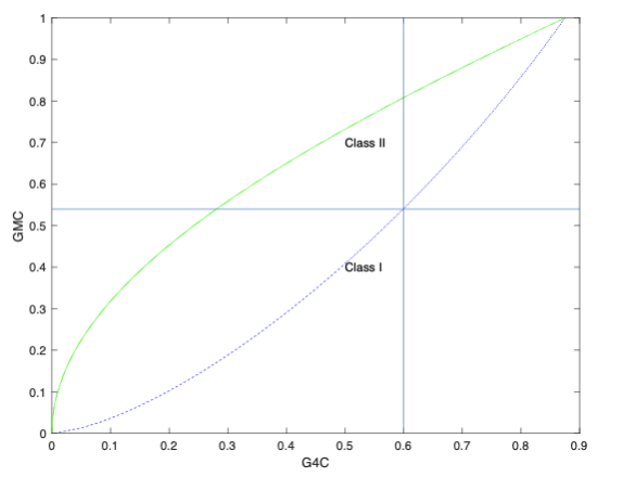
(a) The G4C and GMC for the Class I states and Class II states.

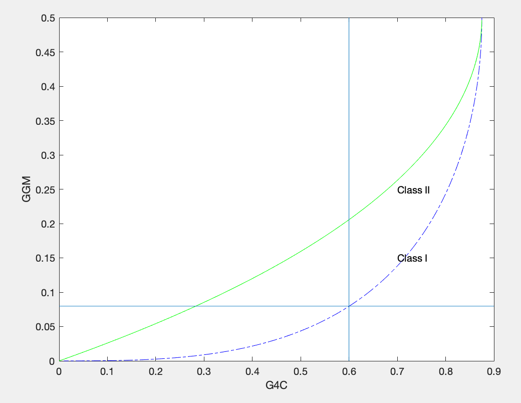
(b) The G4C and GGM for the Class I states and Class II states.

Figure 4: The G4C, GMC and GGM for the Class I states and Class II states.

From the Fig. 4(a), we see that the G4C owns different entanglement order from the GMC. For a given state belonging to the Class I state, there are many states in Class II with larger GMC but with smaller G4C. This can be shown by drawing vertical or horizontal lines, then compare the states at the intersection point. Similarly, from the Fig. 4(b), the entanglement order of G4C is different from GGM. For a given state of the Class I, there are many states in Class II that with larger GGM but with smaller G4C. The opposite results can be arrived at when given a Class II pure state.
At last, we present another class of 4-qubit pure states, which shows the advantages of GqC when comparing with GGM and GMC.

$$|\psi\rangle= \cos\theta|\phi_{1}\rangle+\sin\theta|0111\rangle,\hskip 8.53581pt\theta\in(0,\frac{\pi}{2}),$$ (20)

$$|\phi_{1}\rangle= \cos\frac{2\pi}{3}|0100\rangle+\sin\frac{2\pi}{3}|1000\rangle.$$

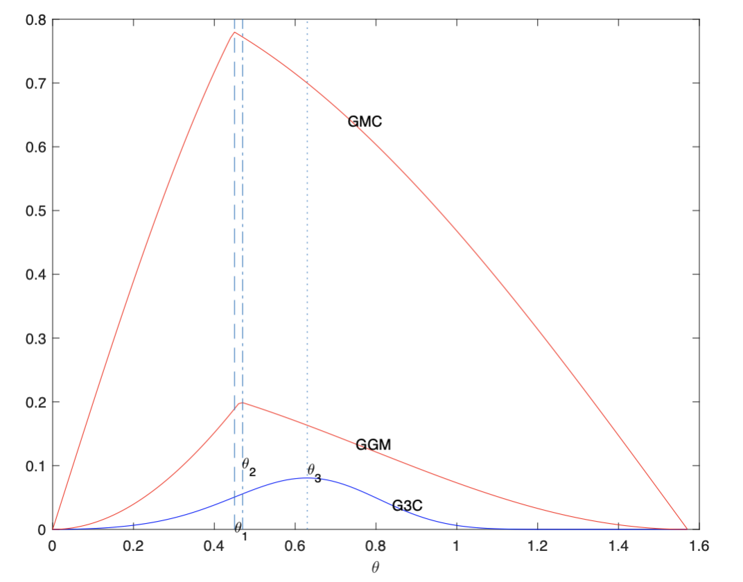
Figure 5: The G3C,GMC and GGM for the four qubit pure states (20).

As presented in Fig.5, when $\theta$ increases from $[\theta_{1},\theta_{3}],$ the values of G3C increases, while the GGM decreases from $[\theta_{2},\theta_{3}]$ and GMC decreases from $[\theta_{1},\theta_{3}].$ Next when $\theta$ ranges in $[0,\theta_{3}],$ each G3C value corresponds to a unique state in the class $(\ref{e12}),$ while there exists pairs of states in the class $(\ref{e12})$ with the same GGM or GBC, that is, the GME measure G3C can detects the robustness between some states while the GGM and GBC cannot. Moreover, Fig. 5 show the smoothness of G3C, a sharp peak appears with the varying $\theta$ when considering the GMC and GGM.

IV Conclusion

In this paper, we have proposed and investigated a GME measure based on the geometric mean method. First we have presented the GqC is a GME measure and satisfies the subadditivity and continuity for pure states. We have also presented the analytical expressions of GqC for the W states and GHZ states in $n$-qubit systems. From the analytical expressions, we can see that the entanglement of the GHZ state is stronger than the W state. Next we have presented a lower bound of the GqC based on the method proposed in dai2020experimentally . At last, we have presented the advantages of the GqC by comparing with the GMC and GGM through some examples. Due to the importance of the study of GME measures, our results can provide a reference for future work on the study of multiparty quantum entanglement.

V Appendix

V.1 Some results on $\mathcal{G}_{q}(|W_{n}\rangle)$ and $\mathcal{G}_{q}(|GHZ_{n}\rangle)$

An $n$-qubit W state can be represented as

$$|W_{n}\rangle=\frac{1}{\sqrt{n}}(|00\cdots 1\rangle+|01\cdots 0\rangle+\cdots+|00\cdots 1\rangle).$$

Through computation, we have

$$\mathcal{C}_{q1,n-1}(|W_{n}\rangle)= 1-\frac{1}{n^{q}}-\frac{(n-1)^{q}}{n^{q}},$$

$$\mathcal{C}_{q,2,n-2}(|W_{n}\rangle)= 1-\frac{2^{q}}{n^{q}}-\frac{(n-2)^{q}}{n^{q}},$$

$$\cdots, \hskip 5.69054pt\cdots,\hskip 5.69054pt\cdots$$

$$\mathcal{C}_{q,k,n-k}(|W_{n}\rangle)= 1-\frac{k^{q}}{n^{q}}-\frac{(n-k)^{q}}{n^{q}},$$

An $n$-qubit GHZ state can be represented as

$$|GHZ_{n}\rangle=\frac{1}{\sqrt{2}}(|00\cdots 0\rangle+|11\cdots 1\rangle).$$

Through computation, we have

$$\mathcal{C}_{q,k,n-k}(|GHZ_{n}\rangle)=1-\frac{1}{2^{q-1}},$$

then we have

$$\mathcal{G}_{q}(|W_{n}\rangle)=\begin{split}\left\{\begin{array}[]{lr}(\Pi_{k=1}^{\frac{n-1}{2}}[1-\frac{k^{q}}{n^{q}}-\frac{(n-k)^{q}}{n^{q}}]^{C_{n}^{k}})^{\frac{1}{c(\alpha)}},\hskip 8.53581pt\textit{if $n$ is odd,}\\ (\Pi_{k=1}^{\frac{n}{2}-1}[1-\frac{k^{q}}{n^{q}}-\frac{(n-k)^{q}}{n^{q}}]^{C_{n}^{k}}[1-\frac{1}{2^{q-1}}]^{\frac{C_{n}^{\frac{n}{2}}}{2}})^{\frac{1}{c(\alpha)}},\hskip 8.53581pt\textit{if $n$ is even.}\end{array}\right.\end{split}$$

$$\frac{\mathcal{G}_{q}(|W_{n}\rangle)}{\mathcal{G}_{q}(|GHZ_{n}\rangle)}=\begin{split}\left\{\begin{array}[]{lr}\frac{\exp[\frac{\sum_{k=1}^{\frac{n-1}{2}}C_{n}^{k}}{c(\alpha)}(\ln(1-\frac{k^{q}}{n^{q}}-\frac{(n-k)^{q}}{n^{q}}))]}{1-\frac{1}{2^{q-1}}},\hskip 8.53581pt\textit{if $n$ is odd,}\\ \frac{\exp[\frac{\sum_{k=1}^{\frac{n}{2}-1}C_{n}^{k}}{c(\alpha)}\ln(1-\frac{k^{q}}{n^{q}}-\frac{(n-k)^{q}}{n^{q}})+\frac{\frac{C_{n}^{\frac{n}{2}}}{2}\ln(1-\frac{1}{2^{q-1}})}{c(\alpha)}]}{1-\frac{1}{2^{q-1}}},\hskip 8.53581pt\textit{if $n$ is even.}\end{array}\right.\end{split}$$

Then by using the Stolz-Cresaro theorem, we have

$$\lim_{k\rightarrow\infty}\frac{\mathcal{G}_{q}(|W_{2k}\rangle)}{\mathcal{G}_{q}(|GHZ_{2k}\rangle)}=1,$$

$$\lim_{k\rightarrow\infty}\frac{\mathcal{G}_{q}(|W_{2k+1}\rangle)}{\mathcal{G}_{q}(|GHZ_{2k+1}\rangle)}=1.$$

V.2 The proof on the continuity of $\mathcal{G}_{q}(\cdot)$ for pure states

Here we present the proof of Lemma 5.

Lemma 5: Assume $|\psi_{1}\rangle$ and $|\psi_{2}\rangle$ are pure states in $\mathcal{H}_{d}\otimes\mathcal{H}_{d},$ when $\lVert|\psi_{1}\rangle-|\psi_{2}\rangle\rVert_{1}\leq\epsilon$, then we have

$$|\mathcal{C}_{q}(|\psi_{1}\rangle)-\mathcal{C}_{q}(|\psi_{2}\rangle)|\leq d[(1+\frac{\epsilon}{d})^{q}-1].$$ (21)

Proof.

As partial trace is trace-preserving, then $\lVert\rho_{A}-\sigma_{A}\rVert_{1}\leq\epsilon,$ here $\rho_{A}=Tr_{B}|\psi\rangle\langle\psi|$, $\sigma_{A}=Tr_{B}|\sigma\rangle\langle\sigma|.$

Next as $\lVert\cdot\rVert_{1}$ is unitarily invariant norm, then

$$\lVert Eig^{\downarrow}(\rho_{A})-Eig^{\downarrow}(\sigma_{A})\rVert\leq\lVert\rho_{A}-\sigma_{A}\rVert_{1},$$

$$\lVert\rho_{A}-\sigma_{A}\rVert_{1}\leq\lVert Eig^{\downarrow}(\rho_{A})-Eig^{\uparrow}(\sigma_{A})\rVert,$$

that is, we only need to consider the classical case. Readers who are interesting in the above two inequalities please refer to bhatia2013matrix .

Assume $\rho_{A}$ and $\sigma_{A}$ are two diagonal density matrices with their diagonal elements are $\{p_{i}\}_{i=1}^{d}$ and $\{r_{i}\}_{i=1}^{d},$ respectively. And $\{p_{i}\}_{i=1}^{d}$ and $\{r_{i}\}_{i=1}^{d}$ satisfy $\sum_{i}p_{i}=\sum_{i}r_{i}=1,$ and $\sum_{i}|p_{i}-r_{i}|\leq\epsilon.$ Then

$$|\mathcal{C}_{q}(\rho_{A})-\mathcal{C}_{q}(\sigma_{A})|= |\mathop{\rm Tr}\rho_{A}^{q}-\mathop{\rm Tr}\sigma_{A}^{q}|$$

$$\leq \sum_{i}|p_{i}^{q}-r^{q}_{i}|$$ (22)

Next let $|p_{i}-r_{i}|=\epsilon_{i}$, $\sum_{i}\epsilon_{i}\leq\epsilon,$ when $p_{i}=r_{i}+\epsilon_{i},$ then

$$|p_{i}^{q}-r_{i}^{q}|= |(r_{i}+\epsilon_{i})^{q}-r_{i}^{q}|$$

$$\leq (1+\epsilon_{i})^{q}-1,$$

the last inequality is due to that $(r_{i}+\epsilon_{i})^{q}-r_{i}^{q}$ is increasing in terms of $r_{i}$, and $r_{i}\in(0,1).$ And due to that $(r_{i}+\epsilon_{i})^{q}-r_{i}^{q}$ is increasing in terms of $r_{i}$, when $p_{i}=r_{i}-\epsilon_{i}$, the above inequality is also valid. Then the inequality $(\ref{in1})$ becomes

$$(\ref{in1})=\sum_{i}|p_{i}^{q}-r^{q}_{i}|\leq \epsilon^{q}\frac{\sum_{i}[(1+\epsilon_{i})^{q}-1]}{\epsilon^{q}}$$

$$\leq d[(1+\frac{\epsilon}{d})^{q}-1],$$ (23)

when all $\epsilon_{i}=\frac{\epsilon}{d}$, the equality in the last inequality is valid.     $\sqcap$$\sqcup$

Theorem 6: Assume $|\psi_{1}\rangle$ and $|\psi_{2}\rangle$ are two pure states in $n$-partite systems $\mathcal{H}_{d}\otimes\mathcal{H}_{d}\otimes\cdots\otimes\mathcal{H}_{d}$, here $\lVert|\psi_{1}\rangle-|\psi_{2}\rangle\rVert\leq\epsilon,$ then we have

$$|\mathcal{G}_{q}(|\psi_{1}\rangle)-\mathcal{G}_{q}(|\psi_{2}\rangle)|\leq[\sum_{i=1}^{\frac{n-1}{2}}C_{n}^{i}d^{i}[(1+\frac{\epsilon}{d^{i}})^{q}-1]]^{\frac{1}{c(\alpha)}}$$ (24)

Proof.

When $n$ is odd, then we have

$$|\mathcal{G}_{q}(|\psi_{1}\rangle)-\mathcal{G}_{q}(|\psi_{2}\rangle)|$$

$$= |\mathcal{P}_{q}(|\psi_{1}\rangle)^{\frac{1}{c(\alpha)}}-\mathcal{P}_{q}(|\psi_{2}\rangle)^{\frac{1}{c(\alpha)}}|$$

$$\leq |\mathcal{P}_{q}(|\psi_{1}\rangle)-\mathcal{P}_{q}(|\psi_{2}\rangle)|^{\frac{1}{c(\alpha)}}$$

$$= |\Pi_{\alpha_{i}\in\alpha}\mathcal{C}_{qA_{\alpha_{i}}B_{\alpha_{i}}}(|\psi_{1}\rangle)-\Pi_{\alpha_{i}\in\alpha}\mathcal{C}_{qA_{\alpha_{i}}B_{\alpha_{i}}}(|\psi_{2}\rangle)|^{\frac{1}{c(\alpha)}}$$

$$\leq [\sum_{i=1}^{\frac{n-1}{2}}C_{n}^{i}d^{i}[(1+\frac{\epsilon}{d^{i}})^{q}-1]]^{\frac{1}{c(\alpha)}}.$$ (25)

the first inequality is due to that when $p,q,x\in(0,1)$, $|p^{x}-q^{x}|\leq|p-q|^{x}$, the second inequality is due to the following inequality, when $x_{i},y_{i}\in(0,1),$ $i=1,2,\cdots,n,$ then we have

$$|x_{1}x_{2}\cdots x_{n}-y_{1}y_{2}\cdots y_{n}|$$

$$= |(x_{1}-y_{1})x_{2}x_{3}\cdots x_{n}+y_{1}(x_{2}-y_{2})x_{3}\cdots x_{n}$$

$$\hskip 2.84526pt+ y_{1}y_{2}(x_{3}-y_{3})x_{4}x_{5}\cdots x_{n}\cdots+y_{1}y_{2}\cdots y_{n-1}(x_{n}-y_{n})|$$

$$\leq \sum_{i}|x_{i}-y_{i}|,$$ (26)

here the last inequality is due to the triangle inequality and $x_{i},y_{i}\in(0,1).$     $\sqcap$$\sqcup$

V.3 The proof of Theorem 7

Here we prove Theorem 7 based on the method in zhang2016evaluation .

Theorem 7: For a bipartite mixed state $\rho$ on the system $\mathcal{H}_{m}\otimes\mathcal{H}_{n}(m\leq n)$, its revised parametrized entanglement measure $\mathcal{C}_{q}(\rho)$ satisfies

$$\mathcal{C}_{q}(\rho)\geq co[R(\Lambda)],$$ (27)

where $\Lambda=\mathop{\rm max}\{\frac{\langle\phi|\rho|\phi\rangle}{s_{1}m},\frac{1}{m}\}$, $R(\Lambda)=1-\gamma(\Lambda)^{q}-\frac{[1-\gamma(\Lambda)]^{q}}{(m-1)^{q-1}},$ with $\gamma(\Lambda)=\frac{\sqrt{\Lambda}+\sqrt{(m-1)(1-\Lambda)}}{m}$, and

$$co[R(\Lambda)]=\frac{m^{q-1}-1}{m^{q-2}(m-1)}(\Lambda-\frac{1}{m}).$$

Proof.

Here we consider the following function

$$R(\lambda)=\mathop{\rm min}_{\vec{\mu}}\{L(\vec{\mu})|\lambda=\frac{1}{m}(\sum_{i}\sqrt{\mu_{i}})^{2}\}.$$ (28)

Here $L(\vec{\mu})=1-\sum_{i}\mu_{i}^{2}$. Due to the results in terhal2000entanglement ; berry2003bounds , the minimum $L(\vec{\mu})$ versus $\lambda$ to $\vec{\mu}$ in the form

$$\vec{\mu}=\{t,\frac{1-t}{m-1},\frac{1-t}{m-1},\cdots,\frac{1-t}{m-1}\}\hskip 8.53581pt\textit{for $t\in[\frac{1}{m},1],$}$$ (29)

Therefore, we have the minimum $L(\vec{\mu})$ and the function $t(\lambda)$ are

$$L(t)= 1-t^{q}-\frac{(1-t)^{q}}{(m-1)^{q-1}},$$ (30)

$$t(\lambda)= \frac{1}{m}(\sqrt{\lambda}+\sqrt{(m-1)(1-\lambda)})^{2},\hskip 8.53581pt\textit{with $\lambda\in[\frac{1}{m},1].$}$$ (31)

Substituting $(\ref{t1})$ into (30), we have

$$L^{{}^{\prime}}_{\lambda}=L^{{}^{\prime}}_{t}\times t^{{}^{\prime}}_{\lambda},$$ (32)

through computation, we have

$$L^{{}^{\prime}}_{t}=-qt^{q-1}+\frac{q(1-t)^{q-1}}{(m-1)^{q-1}},$$ (33)

$$L_{t}^{{}^{\prime\prime}}=-q(q-1)t^{q-2}-\frac{q(q-1)(1-t)^{q-2}}{(m-1)^{q-1}}\leq 0,$$ (34)

$$t_{\lambda}^{{}^{\prime}}=\frac{1}{m}(\sqrt{\lambda}+\sqrt{(m-1)(1-\lambda)})$$

$$\hskip 56.9055pt\times(\frac{1}{\sqrt{\lambda}}+\frac{1-m}{\sqrt{(m-1)(1-\lambda)}})\leq 0,$$ (35)

as $L_{t}^{{}^{\prime\prime}}\leq 0,$ $\mathop{\rm max}_{t}L^{{}^{\prime}}_{t}=L^{{}^{\prime}}(\frac{1}{m})=0,$ that is $L_{\lambda}^{{}^{\prime}}\geq 0,$ $L(\lambda)$ is an increasing function.

Next we prove $L(\lambda)$ is concave.

$$L_{\lambda}^{{}^{\prime\prime}}=L_{t}^{{}^{\prime\prime}}{t_{\lambda}^{{}^{\prime}}}^{2}+L^{{}^{\prime}}_{t}{t_{\lambda}^{{}^{\prime\prime}}}$$ (36)

and

$$t_{\lambda}^{{}^{\prime\prime}}=-\frac{\sqrt{(m-1)(1-\lambda)}}{2m(1-\lambda)^{2}\lambda^{\frac{3}{2}}}.$$ (37)

Through rough computation,

$$L_{\lambda}^{{}^{\prime\prime}}\leq 0,$$

then we have

$$co[R(\lambda)]=\frac{m^{q}-1}{m^{q-1}(m-1)}(\lambda-\frac{1}{m}).$$ (38)

Next we have

$$\mathcal{C}_{q}(\rho)= \sum_{i}p_{i}\mathcal{C}_{q}(|\psi_{i}\rangle)=\sum_{i}p_{i}L(\vec{\mu^{j}})$$

$$\geq \sum_{i}p_{i}co[R(\lambda^{j})]\geq co[R(\sum_{j}p_{j}\lambda^{j})]\geq co[R(\Lambda)],$$ (39)

where $|\psi_{j}\rangle=U_{A}\otimes U_{B}\sum_{i}\sqrt{\mu_{i}^{j}}|ii\rangle$ with $\sqrt{\mu_{i}^{j}}$ being its Schmidt coefficients in decreaing order. The last inequality is due to that $co{R(\lambda)}$ is an increasing function.     $\sqcap$$\sqcup$

V.4 The proof of Theorem 8

Here we present the proof of Theorem 8.

Theorem 8: Assume $\rho_{A_{1}A_{2}\cdots A_{n}}$ is a mixed state on an $n$-paritite system. Then we have

$$\mathcal{G}_{q}(\rho)\geq\frac{m^{q-1}-1}{m^{q-2}(m-1)}(\Lambda^{{}^{\prime}}-\frac{1}{m}),$$ (40)

here we denote $\Lambda^{{}^{\prime}}=\mathop{\rm max}\{\frac{\langle\phi|\rho|\phi\rangle}{s_{1}m},\frac{1}{m}\}$

Proof.

Assume $\{p_{j},|\phi_{j}\rangle\}$ is the optimal decompostion of the state $\rho$ in terms of $\mathcal{G}_{q}(\rho),$ then we have

$$\mathcal{G}_{q}(\rho)= \sum_{j}p_{j}[\Pi_{\alpha_{i}\in\alpha}\mathcal{C}_{qA_{\alpha_{i}}B_{\alpha_{i}}}(|\phi_{j}\rangle)]^{\frac{1}{c(\alpha)}}$$

$$= \sum_{j}[\Pi_{\alpha_{i}\in\alpha}p_{j}\mathcal{C}_{qA_{\alpha_{i}}B_{\alpha_{i}}}(|\phi_{j}\rangle)]^{\frac{1}{c(\alpha)}}$$

$$\geq \sum_{j}\mathop{\rm min}_{\alpha_{i}\in\alpha}p_{j}\mathcal{C}_{qA_{\alpha_{i}}B_{\alpha_{i}}}(|\phi_{j}\rangle)$$

$$\geq \mathop{\rm min}_{\alpha_{i}\in\alpha}\sum_{j}p_{j}\mathcal{C}_{qA_{\alpha_{i}}B_{\alpha_{i}}}(|\phi_{j}\rangle)$$

$$\geq \frac{m^{q-1}-1}{m^{q-2}(m-1)}(\Lambda^{{}^{\prime}}-\frac{1}{m}),$$ (41)

here we denote $\Lambda^{{}^{\prime}}=\mathop{\rm max}\{\frac{\langle\phi|\rho|\phi\rangle}{s_{1}m},\frac{1}{m}\}.$ The first inequality is due to that $\mathop{\rm min}(x,y)\leq\sqrt{xy},$ $\forall x,y\in[0,1].$ The last inequality is due to the Lemma 5.     $\sqcap$$\sqcup$

References

- (1) R. Horodecki, P. Horodecki, M. Horodecki, and K. Horodecki, “Quantum entanglement,” Reviews of modern physics, vol. 81, no. 2, p. 865, 2009.
- (2) C. H. Bennett and S. J. Wiesner, “Communication via one-and two-particle operators on einstein-podolsky-rosen states,” Physical review letters, vol. 69, no. 20, p. 2881, 1992.
- (3) C. H. Bennett, G. Brassard, C. Crépeau, R. Jozsa, A. Peres, and W. K. Wootters, “Teleporting an unknown quantum state via dual classical and einstein-podolsky-rosen channels,” Physical review letters, vol. 70, no. 13, p. 1895, 1993.
- (4) Y. Shimoni, D. Shapira, and O. Biham, “Entangled quantum states generated by shor’s factoring algorithm,” Physical Review A, vol. 72, no. 6, p. 062308, 2005.
- (5) V. Vedral, M. B. Plenio, M. A. Rippin, and P. L. Knight, “Quantifying entanglement,” Physical Review Letters, vol. 78, no. 12, p. 2275, 1997.
- (6) G. Vidal, “Entanglement monotones,” Journal of Modern Optics, vol. 47, no. 2-3, pp. 355–376, 2000.
- (7) G. Gour and M. Tomamichel, “Optimal extensions of resource measures and their applications,” arXiv preprint arXiv:2006.12408, 2020.
- (8) X. Shi and L. Chen, “An extension of entanglement measures for pure states,” Annalen der Physik, vol. 533, no. 4, p. 2000462, 2021.
- (9) O. Gühne, G. Tóth, and H. J. Briegel, “Multipartite entanglement in spin chains,” New Journal of Physics, vol. 7, no. 1, p. 229, 2005.
- (10) M. B. Plenio and S. S. Virmani, “An introduction to entanglement theory,” in Quantum Information and Coherence. Springer, 2014, pp. 173–209.
- (11) D. A. Meyer and N. R. Wallach, “Global entanglement in multiparticle systems,” Journal of Mathematical Physics, vol. 43, no. 9, pp. 4273–4278, 2002.
- (12) M. Blasone, F. Dell’Anno, S. De Siena, and F. Illuminati, “Hierarchies of geometric entanglement,” Physical Review A, vol. 77, no. 6, p. 062304, 2008.
- (13) B. C. Hiesmayr, M. Huber, and P. Krammer, “Two computable sets of multipartite entanglement measures,” Physical Review A, vol. 79, no. 6, p. 062308, 2009.
- (14) Z.-H. Ma, Z.-H. Chen, J.-L. Chen, C. Spengler, A. Gabriel, and M. Huber, “Measure of genuine multipartite entanglement with computable lower bounds,” Physical Review A, vol. 83, no. 6, p. 062325, 2011.
- (15) B. Jungnitsch, T. Moroder, and O. Gühne, “Taming multiparticle entanglement,” Physical review letters, vol. 106, no. 19, p. 190502, 2011.
- (16) S. H. Rafsanjani, M. Huber, C. J. Broadbent, and J. H. Eberly, “Genuinely multipartite concurrence of n-qubit x matrices,” Physical Review A, vol. 86, no. 6, p. 062303, 2012.
- (17) S. Xie and J. H. Eberly, “Triangle measure of tripartite entanglement,” Physical Review Letters, vol. 127, no. 4, p. 040403, 2021.
- (18) J. L. Beckey, N. Gigena, P. J. Coles, and M. Cerezo, “Computable and operationally meaningful multipartite entanglement measures,” Physical Review Letters, vol. 127, no. 14, p. 140501, 2021.
- (19) Y. Guo, Y. Jia, X. Li, and L. Huang, “Genuine multipartite entanglement measure,” Journal of Physics A: Mathematical and Theoretical, vol. 55, no. 14, p. 145303, 2022.
- (20) Y. Li and J. Shang, “Geometric mean of bipartite concurrences as a genuine multipartite entanglement measure,” Physical Review Research, vol. 4, no. 2, p. 023059, 2022.
- (21) X. Yang, M.-X. Luo, Y.-H. Yang, and S.-M. Fei, “Parametrized entanglement monotone,” Physical Review A, vol. 103, no. 5, p. 052423, 2021.
- (22) S. Hill and W. K. Wootters, “Entanglement of a pair of quantum bits,” Physical review letters, vol. 78, no. 26, p. 5022, 1997.
- (23) W. K. Wootters, “Entanglement of formation of an arbitrary state of two qubits,” Physical Review Letters, vol. 80, no. 10, p. 2245, 1998.
- (24) V. Coffman, J. Kundu, and W. K. Wootters, “Distributed entanglement,” Physical Review A, vol. 61, no. 5, p. 052306, 2000.
- (25) F. Mintert, M. Kuś, and A. Buchleitner, “Concurrence of mixed bipartite quantum states in arbitrary dimensions,” Physical review letters, vol. 92, no. 16, p. 167902, 2004.
- (26) K. Chen, S. Albeverio, and S.-M. Fei, “Concurrence of arbitrary dimensional bipartite quantum states,” Physical review letters, vol. 95, no. 4, p. 040504, 2005.
- (27) C. Zhang, S. Yu, Q. Chen, H. Yuan, and C. Oh, “Evaluation of entanglement measures by a single observable,” Physical Review A, vol. 94, no. 4, p. 042325, 2016.
- (28) Y. Dai, Y. Dong, Z. Xu, W. You, C. Zhang, and O. Gühne, “Experimentally accessible lower bounds for genuine multipartite entanglement and coherence measures,” Physical Review Applied, vol. 13, no. 5, p. 054022, 2020.
- (29) M. Li, Z. Wang, J. Wang, S. Shen, and S.-m. Fei, “Improved lower bounds of concurrence and convex-roof extended negativity based on bloch representations,” Quantum Information Processing, vol. 19, no. 4, pp. 1–11, 2020.
- (30) C. Tsallis, “Possible generalization of boltzmann-gibbs statistics,” Journal of statistical physics, vol. 52, no. 1, pp. 479–487, 1988.
- (31) P. T. Landsberg and V. Vedral, “Distributions and channel capacities in generalized statistical mechanics,” Physics Letters A, vol. 247, no. 3, pp. 211–217, 1998.
- (32) C. Tsallis, S. Lloyd, and M. Baranger, “Peres criterion for separability through nonextensive entropy,” Physical Review A, vol. 63, no. 4, p. 042104, 2001.
- (33) R. Rossignoli and N. Canosa, “Generalized entropic criterion for separability,” Physical Review A, vol. 66, no. 4, p. 042306, 2002.
- (34) J. San Kim, “Tsallis entropy and entanglement constraints in multiqubit systems,” Physical Review A, vol. 81, no. 6, p. 062328, 2010.
- (35) W. Helwig, W. Cui, J. I. Latorre, A. Riera, and H.-K. Lo, “Absolute maximal entanglement and quantum secret sharing,” Physical Review A, vol. 86, no. 5, p. 052335, 2012.
- (36) W. Helwig and W. Cui, “Absolutely maximally entangled states: existence and applications,” arXiv preprint arXiv:1306.2536, 2013.
- (37) M. Grassl and M. Rötteler, “Quantum mds codes over small fields,” in 2015 IEEE International Symposium on Information Theory (ISIT). IEEE, 2015, pp. 1104–1108.
- (38) D. Alsina and M. Razavi, “Absolutely maximally entangled states, quantum-maximum-distance-separable codes, and quantum repeaters,” Physical Review A, vol. 103, no. 2, p. 022402, 2021.
- (39) D. Goyeneche, D. Alsina, J. I. Latorre, A. Riera, and K. Życzkowski, “Absolutely maximally entangled states, combinatorial designs, and multiunitary matrices,” Physical Review A, vol. 92, no. 3, p. 032316, 2015.
- (40) X. Shi, L. Chen, and M. Hu, “Multilinear monogamy relations for multiqubit states,” Physical Review A, vol. 104, no. 1, p. 012426, 2021.
- (41) J. Joo, Y.-J. Park, S. Oh, and J. Kim, “Quantum teleportation via a w state,” New Journal of Physics, vol. 5, no. 1, p. 136, 2003.
- (42) P. Vrana and M. Christandl, “Asymptotic entanglement transformation between w and ghz states,” Journal of Mathematical Physics, vol. 56, no. 2, p. 022204, 2015.
- (43) S. Virmani, M. F. Sacchi, M. B. Plenio, and D. Markham, “Optimal local discrimination of two multipartite pure states,” Physics Letters A, vol. 288, no. 2, pp. 62–68, 2001.
- (44) K. Życzkowski and I. Bengtsson, “Relativity of pure states entanglement,” Annals of Physics, vol. 295, no. 2, pp. 115–135, 2002.
- (45) R. Bhatia, Matrix analysis. Springer Science & Business Media, 2013, vol. 169.
- (46) B. M. Terhal and K. G. H. Vollbrecht, “Entanglement of formation for isotropic states,” Physical Review Letters, vol. 85, no. 12, p. 2625, 2000.
- (47) D. W. Berry and B. C. Sanders, “Bounds on general entropy measures,” Journal of Physics A: Mathematical and General, vol. 36, no. 49, p. 12255, 2003.