How does a Rational Agent Act in an Epidemic?

Abstract

Evolution of disease in a large population is a function of the top-down policy measures from a centralized planner, as well as the self-interested decisions (to be socially active) of individual agents in a large heterogeneous population. This paper is concerned with understanding the latter based on a mean-field type optimal control model. Specifically, the model is used to investigate the role of partial information on an agent’s decision-making, and study the impact of such decisions by a large number of agents on the spread of the virus in the population. The motivation comes from the presymptomatic and asymptomatic spread of the COVID-19 virus where an agent unwittingly spreads the virus. We show that even in a setting with fully rational agents, limited information on the viral state can result in an epidemic growth.

I Introduction

Social behavior of individual agents ultimately drives the case count in an epidemic. Decisions of an individual agent are mediated by the top-down policy guidelines, e.g., lockdown mandates or social distancing guidelines. However, these decisions are also a function of: (i) the agent’s risk-reward trade-off based on the agent’s health condition, age, and information from media on transmissibility and lethality of the virus (e.g., omicron variant is more transmissible but less deadly than the delta variant), (ii) aggregate positivity rate in the local population, and (iii) the agent’s assessment of its own epidemiological status.

This paper is a continuation of prior work from our group on modeling an agent’s decision-making in an epidemic based on mean-field game (MFG) formalisms [1]. The primary focus of the current paper is to investigate the role of agent rationality and information on agent behavior. The motivation comes from the following thought experiment: On the planet of Vulcan, the agents are both perfectly rational and perfectly informed. Because an agent has perfect information, it immediately knows its epidemiological status. And because an agent is perfectly rational, it knows to self-quarantine if infected. Therefore, the rational choice of a susceptible (non-infected) agent is to carry on with normal life. This is because it can count on rational choices of perfectly informed others.

Unfortunately in reality, on the planet of Earth, we continue to experience waves of infection which are doubtlessly caused by emergence of variants but surely exacerbated by our own actions which are often less than rational and certainly almost always based on incomplete information. A case in point is the role played by the presymptomatic and asymptomatic spread of the COVID-19 virus [2, 3, 4, 5].

The contributions of this paper are as follows. Apart from the development of the model, we derive several qualitative insights into an agent’s actions in the midst of an epidemic. Specifically, these insights are related to: (i) the risk-reward tradeoff of a susceptible agent, and (ii) the evolution of belief of an active agent who does not show symptoms. The resulting decision-making and its effect on the disease outbreak in the population are discussed at length. These qualitative insights are drawn from quantitative results presented as part of Props. 3, 4, and 5, and as illustrated in Figs. 3-7. The discussion appears in Sec. IV-D.

Closely related to our work are [6], where an agent’s decision variable is its rate of contact with others, and [7, 8], where an agent strives to follow a prescribed rate of contact based on government guidelines. Other MFG-style modeling of epidemics appears in [9, 10, 11, 12, 13]. The novelty of our work comes from the inherent partial observability of viral status and differences in cost structures. These factors are crucial for modeling the asymptomatic spread of an epidemic.

The remainder of the paper is organized as follows. The problem formulation appears in Sec. II where the two main questions of the paper are also introduced. The answers to these questions are based on the analysis of the HJB equations derived in Sec. III. The analysis is presented in Sec. IV together with qualitative answers to the two main questions. These answers conclude this paper and spur the development of the MFG formalism. This formalism, which will be studied in detail as part of future work, is presented in Sec. V. The proofs appear in the Appendix.

(a)

state	health	alturistic	activity
	cost	cost	reward
	$c^{\text{h}}(x)$	$c^{\text{a}}(x)$	$r(x)$
s	$0$	$0$	$\alpha$
a	$0$	$1$	$\alpha$
i	$1$	$1$	$\alpha$

(b)

Figure 1: (a) Epidemiological states and the associated transition graph. (b) Model for running cost: It is assumed that the economic reward of $\alpha$ is smaller than the altruistic cost of $1$ for an asymptomatic ($x=\textbf{\emph{a}}$) or symptomatic ($x=\textbf{\emph{i}}$) agent.

II Problem Formulation

II-A Model for a Single Agent

Dynamics: The epidemiological state of a single agent is modeled as a Markov process $X:=\{X_{t}\in\mathcal{X}:t\geq 0\}$ with state-space $\mathcal{X}:=\{\textbf{\emph{s}},\textbf{\emph{a}},\textbf{\emph{i}},\textbf{\emph{r}},\textbf{\emph{d}}\}$. Fig. 1 depicts the transition graph along with a description of the epidemiological meaning of each of the five states. Notably, there are two types of infected states: (i) asymptomatic state, denoted as a; and (ii) symptomatic state, denoted as i. In either of these states, an agent is infectious, i.e., able to infect other agents. The modeling distinction is that, in partially observed settings, an asymptomatic agent may not know its true state but a symptomatic agent does. Note that unlike our previous paper [1], the transition graph now includes an edge from a to r. This is more realistic, but significantly complicates modeling and analysis. Broadly, there are two types of transitions:

1) On the subset $\{\textbf{\emph{a}},\textbf{\emph{i}},\textbf{\emph{r}},\textbf{\emph{d}}\}$, the transition rate depends only upon the agent attribute $\theta$, which here represents the age of the agent. For example, an older symptomatic agent has a longer expected recovery time (smaller $\lambda^{\text{\tiny IR}})$ than a younger one.

2) The transition from $\textbf{\emph{s}}\to\textbf{\emph{a}}$ depends upon three factors: (i) the intrinsic infectivity of the virus, (ii) the agent behavior (level of social activity), and (iii) the behavior of the infected agents in the population. The following equation is used to model the effect of these three factors:

$$\text{rate}[\textbf{\emph{s}}\to\textbf{\emph{a}}]=\eta+\lambda^{\text{\tiny SA}}\ \beta_{t}\,U_{t}$$

where $\eta>0$ is a small baseline rate (useful for regularizing the problem) and $\lambda^{\text{\tiny SA}}$ is the virus transmissibility parameter. The process $U$ is referred to as the agent’s control input, and models the agent’s activity level: With $U_{t}=0$ (resp., $U_{t}=1$) the agent is isolated (resp., normally active) at time $t$ (Fig. 2). The process $\beta$ models the average activity level of the infected agents (Eq. (1)).

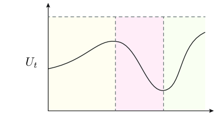
Figure 2: A qualitative representation of the control input. Agents choose their activity levels based on their own viral status and the disease level within the population.

The two main questions driving this work are as follows: (i) How does a single agent choose its control input $U$? and (ii) How does that choice (made by agents) affect the evolution of disease in a large heterogeneous population? To answer these questions, we adopt an optimal control framework.

Optimal control objective: In the following, $\beta$ is a given deterministic process. The control objective for a single agent is to choose its activity $U$ to minimize

$${\sf J}(U;\beta)={\sf E}\left(\int_{0}^{T}e^{-\gamma t}c(X_{t},U_{t})\,\mathrm{d}t+e^{-\gamma T}\phi(X_{T})\right)$$

where $\gamma>0$ is a discounting rate (assumed to be much smaller than the transition rates), $T=T(\omega)=\inf\{t>0:X_{t}(\omega)\in\{\textbf{\emph{d}},\textbf{\emph{r}}\}\}$ is the random stopping time when the agent either recovers ($X_{T}=\textbf{\emph{r}}$) or the agent dies ($X_{T}=\textbf{\emph{d}}$); by convention, $\inf\emptyset=\infty$. The cost function is of the following form:

$$c(x,u) =c^{\text{h}}(x)+\left(c^{\text{a}}(x)-r(x)\right)u$$

where $c^{\text{h}}(\cdot)$, $c^{\text{a}}(\cdot)$, and $r(\cdot)$ model the health cost, altruistic cost, and economic reward, respectively (Fig. 1 (b)). The altruistic cost models an agent’s desire to help the greater good and has the effect of inducing an infected agent to isolate. Of course, an agent’s choice is mediated by its information, the structure of which is described next.

Information structure: There are two settings of the problem: (i) the fully observed case, and (ii) the partially observed case. In the partially observed setting, the observation process $Y:=\{Y_{t}\in\{0,1,2\}:t\geq 0\}$ is defined as

$$Y_{t}=1_{[X_{t}=\textbf{\emph{i}}]}+2\cdot 1_{[X_{t}=\textbf{\emph{d}}]}$$

Therefore, an infected agent who is also asymptomatic (in state a) does not observe its epidemiological status until it begins to show symptoms (in state i).

II-B Model for the Mean-Field

To fully specify the problem, we need to define the model for the agent’s attribute $\theta$ and the process $\beta$, henceforth referred to as the mean-field process. The probability mass function of the attribute $\theta$ is denoted by ${\sf p}(\cdot)$. Denote by $\rho_{t}(x,u;\theta)$ the joint distribution of the state-action pair $(X_{t},U_{t})$ at time $t$, conditioned on the attribute $\theta$. At time $t$, the average activity level of infected agents is

$$\beta_{t}:=\sum_{\theta}{\sf p}(\theta)\sum_{x\in\{\textbf{\emph{a}},\textbf{\emph{i}}\}}\int_{0}^{1}u\rho_{t}(x,u;\theta)\,\mathrm{d}u\\$$ (1)

which we define to be the mean-field process.

II-C Function Spaces

The filtration of the Markov process $X$ is denoted by ${\cal F}:=\{{\cal F}_{t}:t\geq 0\}$ where ${\cal F}_{t}:=\sigma(X_{t})$. The filtration of the observation process $Y$ is denoted by ${\cal Y}:=\{{\cal Y}_{t}:t\geq 0\}$ where ${\cal Y}_{t}:=\sigma(\{Y_{s}:0\leq s\leq t\})$. In the two settings of the problem, the spaces of admissible control inputs, denoted by ${\cal U}$ in each case, are as follows:

$$\text{(fully obsvd.)}\qquad{\cal U} =L^{2}_{\cal F}([0,\infty);[0,1])$$

$$\text{(part. obsvd.)}\qquad{\cal U} =L^{2}_{\cal Y}([0,\infty);[0,1])\$$

i.e., an admissible control input $U$ is a $[0,1]$-valued stochastic process adapted to ${\cal F}$ in the fully observed case, and adapted to ${\cal Y}$ in the partially observed case. The use of the common notation ${\cal U}$ should not cause any confusion because the two cases are treated in separate subsections. The process $\beta$ is assumed to be deterministic. The function space for $\beta$ is ${\cal M}=L^{2}([0,\infty);[0,1])$.

III Optimality equations for a single agent

III-A Fully Observed Case

For each $x\in\mathcal{X}$ and $t\geq 0$, the value function is

$$v_{t}(x):=\min_{U\in L^{2}_{\cal F}}$$

$${\sf E}\left(\left.\int_{t}^{T}e^{-\gamma(s-t)}c(X_{s},U_{s})\mathop{}\!\mathrm{d}s+e^{-\gamma T}\phi(X_{T})\right|X_{t}=x\right)$$ (2)

where at the two terminal states $x=\textbf{\emph{d}}$ and $x=\textbf{\emph{r}}$, the value function is given by known constants $v_{t}(\textbf{\emph{d}})=\bar{\phi}(\textbf{\emph{d}})$ and $v_{t}(\textbf{\emph{r}})=\bar{\phi}(\textbf{\emph{r}})$.

For the fully observed problem, complete characterizations of the value function and the optimal control are described in the following proposition. This result is a minor extension of a similar result appearing in our prior paper [1] (for $\lambda^{\text{\tiny AR}}$ and $\eta=0$) and therefore its proof is omitted.

Proposition 1

Suppose $\alpha<1$. For $x\in\{\textbf{\emph{a}},\textbf{\emph{i}},\textbf{\emph{r}},\textbf{\emph{d}}\}$, the value function $v_{t}(x)$ and the optimal control law $\psi_{t}(x)$ are stationary as tabulated in Table I. For state s, the value function $v_{t}(\textbf{\emph{s}})$ solves the HJB equation

$$-\frac{\,\mathrm{d}v_{t}}{\,\mathrm{d}t}(\textbf{\emph{s}}) +(\gamma+\eta)v_{t}(\textbf{\emph{s}})$$

$$=\eta\bar{\phi}(\textbf{\emph{a}})+\min_{u\in[0,1]}\left(\lambda^{\text{\tiny SA}}\beta_{t}\left(\bar{\phi}(\textbf{\emph{a}})-v_{t}(\textbf{\emph{s}})\right)-\alpha\right)u$$

state $x$	value function $v_{t}(x)$	optimal control
a	$\frac{c^{h}(\textbf{\emph{a}})+\lambda^{\text{\tiny AI}}\bar{\phi}(\textbf{\emph{i}})+\lambda^{\text{\tiny AR}}\bar{\phi}(\textbf{\emph{r}})}{\gamma+\lambda^{\text{\tiny AI}}+\lambda^{\text{\tiny AR}}}$ $=:\bar{\phi}(\textbf{\emph{a}})$	$U_{t}^{\text{opt}}=\psi_{t}(\textbf{\emph{a}})=0$
i	$\frac{c^{h}(\textbf{\emph{i}})+\lambda^{\text{\tiny IR}}\bar{\phi}(\textbf{\emph{r}})+\lambda^{\text{\tiny ID}}\bar{\phi}(\textbf{\emph{d}})}{\gamma+\lambda^{\text{\tiny IR}}+\lambda^{\text{\tiny ID}}}$ $=:\bar{\phi}(\textbf{\emph{i}})$	$U_{t}^{\text{opt}}=\psi_{t}(\textbf{\emph{i}})=0$
r	$\bar{\phi}(\textbf{\emph{r}})$ (given)	-
d	$\bar{\phi}(\textbf{\emph{d}})$ (given)	-

TABLE I: Fully observed case.

Remark 1

The optimal control for both asymptomatic and symptomatic agents is zero. This is entirely because $\alpha<1$. Recall that $\alpha$ is a model for economic reward per unit time. The assumption $\alpha<1$ means that the economic reward ($\alpha$) is outweighed by the altruistic cost ($1$).

III-B Partially Observed Case

The partially observed problem is first converted to a fully observed one by introducing the belief state, as in [14, 15], which at time $t$ is denoted by

$$\pi_{t}:=\begin{bmatrix}\pi_{t}(\textbf{\emph{s}})&\pi_{t}(\textbf{\emph{a}})&\pi_{t}(\textbf{\emph{i}})&\pi_{t}(\textbf{\emph{r}})&\pi_{t}(\textbf{\emph{d}})\end{bmatrix}$$

where $\pi_{t}(x):={\sf P}([X_{t}=x]\mid{\cal Y}_{t})$ for $x\in\mathcal{X}$. Since the events $[X_{t}=\textbf{\emph{i}}]$ and $[X_{t}=\textbf{\emph{d}}]$ are both contained in ${\cal Y}_{t}$, $\pi_{t}$ is not an arbitrary element of the probability simplex in $\mathbb{R}^{5}$. Let ${\cal P}^{1}$ denote the set of pmfs on $\{\textbf{\emph{s}},\textbf{\emph{a}},\textbf{\emph{r}}\}$ and let ${\cal P}^{2}=\{\delta_{\textbf{\emph{i}}},\delta_{\textbf{\emph{r}}},\delta_{\textbf{\emph{d}}}\}$. Then, the state-space for the belief is ${\cal P}^{1}\cup{\cal P}^{2}$. For $t\geq 0$ and $\mu\in{\cal P}^{1}\cup{\cal P}^{2}$, the value function is

$$v_{t}(\mu):=\min_{U\in L^{2}_{\cal Y}}$$

$${\sf E}\left(\int_{t}^{T}e^{-\gamma(s-t)}c(X_{s},U_{s};\alpha){\rm d}s+e^{-\gamma T}\phi(X_{T})\mid\pi_{t}=\mu\right)$$

There are two cases to consider: (i) when $\mu\in{\cal P}^{2}$, and (ii) when $\mu\in{\cal P}^{1}\setminus\{\delta_{\textbf{\emph{r}}}\}$. In the first case, when $\mu\in{\cal P}^{2}$, the problem reduces to the fully-observed setting, and the value function is given by

$$v_{t}(\delta_{\textbf{\emph{d}}})=\bar{\phi}(\textbf{\emph{d}}),\;\;v_{t}(\delta_{\textbf{\emph{r}}})=\bar{\phi}(\textbf{\emph{r}}),\;\;v_{t}(\delta_{\textbf{\emph{i}}})=\bar{\phi}(\textbf{\emph{i}})$$

The optimal control for the agent in the symptomatic state ($\pi_{t}=\delta_{\textbf{\emph{i}}}$) is $U_{t}^{\text{opt}}=\psi_{t}(\delta_{\textbf{\emph{i}}})=0$.

For the second case, when $\mu\in{\cal P}^{1}\setminus\{\delta_{\textbf{\emph{r}}}\}$, a nonlinear filter is used to obtain the evolution of the belief. For this purpose, consider first the random variable $\tau=\tau(\omega)=\inf\{t>0:X_{t}(\omega)=\textbf{\emph{i}}\}$. Now, $\tau$ is a ${\cal Y}_{t}$-stopping time and

$$\pi_{t}=\begin{bmatrix}\pi_{t}(\textbf{\emph{s}})&\pi_{t}(\textbf{\emph{a}})&0&\pi_{t}(\textbf{\emph{r}})&0\end{bmatrix}\quad\text{for}\;\;t<\tau$$

Let $S_{t}:=\pi_{t}(\textbf{\emph{s}})$, $A_{t}:=\pi_{t}(\textbf{\emph{a}})$ and $R_{t}:=\pi_{t}(\textbf{\emph{r}})$ for $t<\tau$. Then the stochastic process $\{(S_{t},A_{t},R_{t})\in[0,1]^{3}:S_{t}+A_{t}+R_{t}=1,0\leq t<\tau\}$ evolves according to the nonlinear filter

$$\frac{\,\mathrm{d}S_{t}}{\,\mathrm{d}t} =\left(-\lambda^{\text{\tiny SA}}\beta_{t}U_{t}-\eta+A_{t}\lambda^{\text{\tiny AI}}\right)S_{t}$$ (3a)

$$\frac{\,\mathrm{d}A_{t}}{\,\mathrm{d}t} =\left(\lambda^{\text{\tiny SA}}\beta_{t}U_{t}+\eta\right)S_{t}+A_{t}\left(-\lambda^{\text{\tiny AI}}-\lambda^{\text{\tiny AR}}+\lambda^{\text{\tiny AI}}A_{t}\right)$$ (3b)

$$\frac{\,\mathrm{d}R_{t}}{\,\mathrm{d}t} =A_{t}(\lambda^{\text{\tiny AR}}+\lambda^{\text{\tiny AI}}R_{t})$$ (3c)

which is derived from the general form detailed by [16].

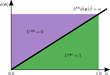
Figure 3: A susceptible agent’s risk-reward diagram. The line $\lambda^{\tiny\text{SA}}\bar{\phi}(\textbf{\emph{a}})\bar{\beta}=\alpha$ is where the risk equals the reward.

We identify ${\cal P}^{1}$ with the domain $D:=\{(s,a)\in[0,1]^{2}:s+a\leq 1\}$ where $s$ is the value of $S_{t}$ and $a$ is the value of $A_{t}$. For an arbitrary element $\mu=[s,a,0,1-s-a,0]$ in ${\cal P}^{1}$, we denote the value function with respect to the $(s,a)$-coordinates as

$$\phi_{t}(s,a):=v_{t}(\mu),\quad(s,a)\in D,\quad t\geq 0$$

The following proposition provides the HJB equation whose derivation appears in Appendix -E.

Proposition 2

The value function $\phi_{t}(s,a)$ solves the HJB equation

$$\left(-\frac{\partial\phi_{t}}{\partial t}+\gamma\phi_{t}\right)(s,a)=({\cal L}\phi_{t})(s,a)+\min_{u\in[0,1]}{\cal M}_{t}(s,a)u$$ (4)

together with boundary conditions

$$\phi_{t}(s,a)-\phi_{t}(s,1-s-a)=(2a+s-1)\left(\bar{\phi}(\textbf{\emph{a}})-\bar{\phi}(\textbf{\emph{r}})\right)$$ (5a)

$$\phi_{t}(0,a)=a\bar{\phi}(\textbf{\emph{a}})+(1-a)\bar{\phi}(\textbf{\emph{r}})$$ (5b)

where the formulae for the linear operators ${\cal L}$ and ${\cal M}_{t}$ appear in Appendix -E.

In the remainder of this paper, it is assumed that a unique solution for the HJB equation exists and yields a well-posed optimal control law, denoted as $\psi_{t}(s,a)$ for $(s,a)\in D$.

IV Analysis of the decision-making by an agent

In this section, an analysis of the HJB and the nonlinear filter equations is given. The analysis is used to develop insights into the decisions of a single agent in an epidemic (given $\beta$). To aid the analysis, it is assumed that $\beta_{t}=\bar{\beta}$ for all $t\geq 0$ (i.e. stationary). The main results are described in the form of three propositions (Props. 3-5) and illustrated with accompanying figures (Fig. 3- 7). The section concludes with a qualitative discussion of an agent’s decision-making in Sec. IV-D.

IV-A Risk-Reward Tradeoff for a Fully Observed Susceptible Agent

Proposition 3 (Stationary Solution)

Suppose $\alpha<1$, $\gamma>0$, $\bar{\phi}(\textbf{\emph{i}})>0$, $\beta_{t}\equiv\bar{\beta}$. Set $\bar{\beta}^{\text{\tiny crit}}:=\frac{\alpha}{\lambda^{\text{\tiny SA}}\bar{\phi}(\textbf{\emph{a}})}\left(1+\frac{\eta}{\gamma}\right)$. Then the optimal control for a susceptible agent is stationary and described by the following cases:

1. If $\bar{\beta}<\bar{\beta}^{\text{\tiny crit}}$, then the optimal control $U_{t}^{\text{opt}}=\psi_{t}(\textbf{\emph{s}})=1$ and the optimal value $v_{t}(\textbf{\emph{s}})=\frac{(\lambda^{\text{\tiny SA}}\bar{\beta}+\eta)\bar{\phi}(\textbf{\emph{a}})-\alpha}{\lambda^{\text{\tiny SA}}\bar{\beta}+\gamma+\eta}$.

2. If $\bar{\beta}\geq\bar{\beta}^{\text{\tiny crit}}$, then the optimal control $U_{t}^{\text{opt}}=\psi_{t}(\textbf{\emph{s}})=0$ and the optimal value $v_{t}(\textbf{\emph{s}})=\frac{\eta}{\gamma+\eta}\bar{\phi}(\textbf{\emph{a}})$.

Remark 2

A susceptible agent’s decision is best understood using a risk-reward diagram depicted in Fig. 3. The horizontal axis of this diagram is the economic reward per unit time ($\alpha$). The vertical axis is the potential health cost (value function $\bar{\phi}(\textbf{\emph{a}})$). The diagram helps show that the optimal decision for an agent is to be active if the reward is greater than the risk. For any given $\alpha$ and $\bar{\phi}(\textbf{\emph{a}})$, the risk-reward analysis reveals a critical threshold $\bar{\beta}^{\text{\tiny crit}}$ above which the agent ceases to be active. It is noted that the critical threshold scales inversely with the product $\lambda^{\text{\tiny SA}}\bar{\phi}(\textbf{\emph{a}})$. This is useful in several ways for analysis:

1. An older agent will have a greater potential health cost $\bar{\phi}(\textbf{\emph{a}})$ and therefore a smaller critical threshold $\bar{\beta}^{\text{\tiny crit}}$.

2. A more contagious (high $\lambda^{\text{\tiny SA}}$) variant may still have a larger critical threshold, if it is significantly less severe (low $\bar{\phi}(\textbf{\emph{a}})$). For instance, the omicron variant is two times more transmissible ($2\times$ greater $\lambda^{\text{\tiny SA}}$) than the delta variant [17]. However, the potential health cost $\bar{\phi}(\textbf{\emph{a}})$ of the omicron is also smaller (because it is less lethal).

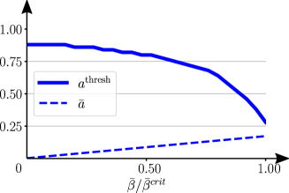
Figure 4: Plot of $a^{\text{\tiny thresh}}$ and $\bar{a}$ as a function of $\bar{\beta}/\bar{\beta}^{\text{crit}}$.

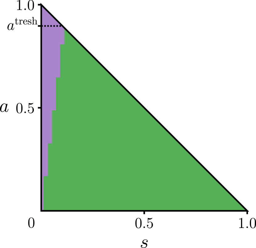
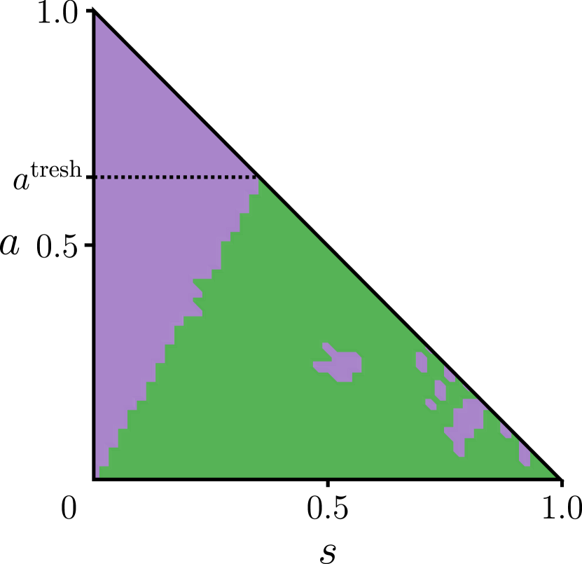
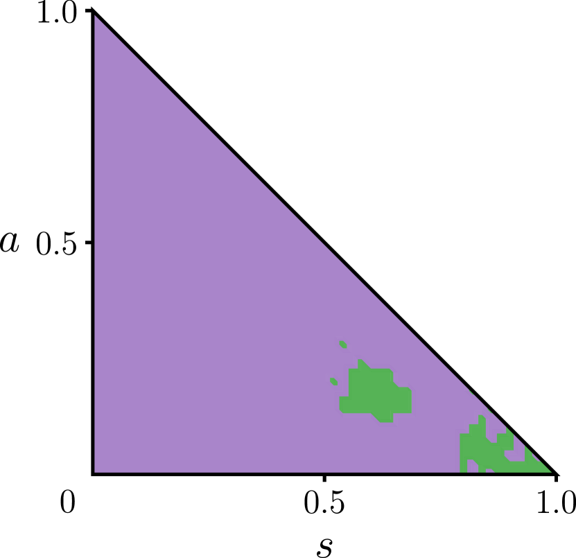
Figure 5: Stationary optimal control policies for the partially observed case; $\alpha=0.9$ and $\bar{\beta}/\beta^{\text{crit}}=0.1,0.8,1.1$ for the three plots. Purple region is $U^{\text{opt}}=0$ and the green region is $U^{\text{opt}}=1$. The islands are numerical artifacts.

IV-B Threshold Optimal Policies for Partially Observed Case

In our prior paper [1], we derived the following result for the solutions of the HJB equation in a special case:

Proposition 4

Suppose $\beta_{t}\equiv\bar{\beta}$, $S_{0}+A_{0}=1$, and $\lambda^{\text{\tiny AR}}=0$. Then, for $t<\tau$, $S_{t}+A_{t}=1$, and

1. If $\bar{\beta}\geq\bar{\beta}^{\text{crit}}$, then the optimal control law ${\bar{\psi}}(\cdot,a)=0$.

2. For each fixed $\bar{\beta}<\frac{\alpha}{\lambda^{\text{\tiny SA}}\bar{\phi}(\textbf{\emph{i}})}<\bar{\beta}^{\text{crit}}$ there exists a $\underline{\lambda}^{\text{\tiny AI}}=\underline{\lambda}^{\text{\tiny AI}}(\bar{\beta})$ such that for all $\lambda^{\text{\tiny AI}}>\underline{\lambda}^{\text{\tiny AI}}$, the optimal control law is of threshold type:

   $$\bar{\psi}(\cdot,a)=\begin{cases}1&\text{if}\;\;0\leq a<{a}^{\text{thresh}}\\ 0&\text{if}\;\;{a}^{\text{thresh}}<a\leq 1\end{cases}$$

   where the threshold ${a}^{\text{thresh}}\in(0,1)$. Furthermore $\lambda^{\text{\tiny SA}}\bar{\beta}/\lambda^{\text{\tiny AI}}<{a}^{\text{thresh}}$. The function $\underline{\lambda}^{\text{\tiny AI}}(\bar{\beta})$ is monotonic in its argument and $\lim_{\bar{\beta}\downarrow 0}\underline{\lambda}^{\text{\tiny AI}}(\bar{\beta})=0$.

With $\lambda^{\text{\tiny AR}}>0$, an analytical treatment has so far not been possible. However, numerical evidence suggests that the policies are also of threshold type even with $\lambda^{\text{\tiny AR}}>0$. Three such numerically obtained stationary policies are depicted in Fig. 5. The policies were computed using the method of lines numerical algorithm described in Appendix -F. From these numerically computed policies, a threshold of ${a}^{\text{thresh}}$ is identified such that an agent becomes inactive for $A_{t}>{a}^{\text{thresh}}$ (see Fig. 5). By identifying the thresholds for different choices of $\bar{\beta}<\bar{\beta}^{\text{\tiny crit}}$, a plot of ${a}^{\text{thresh}}$ as a function of $\frac{\bar{\beta}}{\bar{\beta}^{\text{\tiny crit}}}$ is obtained as depicted in Fig. 4. As $\bar{\beta}\uparrow\bar{\beta}^{\text{\tiny crit}}$, the threshold ${a}^{\text{thresh}}\downarrow 0$ and the agent ceases to be active.

IV-C Belief of an Active Agent who Shows No Symptoms

The analysis thus far has revealed two important insights captured by the critical value for $\bar{\beta}$ and the threshold for $a$:

1. A susceptible agent in the fully observed case is active if $\bar{\beta}$ is small enough ($\bar{\beta}<\bar{\beta}^{\text{\tiny crit}}$).

2. In the absence of symptoms, a partially observed agent is active if its belief $A_{t}$ is small enough ($A_{t}<{a}^{\text{thresh}}$).

Therefore, to determine the actions of an agent in the partially observed case, it becomes important to understand the evolution of the process $\{A_{t}:0\leq t<\tau\}$. This is the subject of the following proposition.

Proposition 5

Set $\bar{a}:=\frac{\lambda^{\text{\tiny SA}}\bar{\beta}+\eta}{\lambda^{\text{\tiny AI}}}$. Suppose $t<\tau$, and

$$S_{0} =1\qquad$$ (agent starts out as susceptible)

$$U_{s} =1\quad\forall\;s<t\quad \text{(agent has been active upto time}\;t\text{)}$$

Then,

$$A_{t}<\bar{a},\qquad 0\leq t<\tau$$

Moreover if $\lambda^{\text{\tiny AR}}=0$, then $A_{t}\uparrow\bar{a}$ as $t\to\infty$.

A numerical illustration of the result of this proposition appears as part of Fig. 6. The most important point about this plot is that the agent’s belief that it is asymptomatic scales as $\eta+\mathcal{O}(\bar{\beta})$.

IV-D Qualitative Discussion

We are now ready to provide a qualitative answer to the two primary questions we had raised: (i) How does a single agent choose its control input $U$?; and (ii) How does that choice (made individually and independently by many agents) affect the evolution of disease in a large heterogeneous population?

The answer to the first question is as follows:

1. In the fully observed setting, a susceptible agent is active if $\bar{\beta}<\bar{\beta}^{\text{\tiny crit}}$. In this setting, an asymptomatic agent isolates (Table I).

2. In the partially observed setting, an agent’s decision is based on its belief $(S_{t},A_{t},R_{t})$. An agent who starts out as susceptible and active has a belief $A_{t}<\bar{a}=\eta+\mathcal{O}(\bar{\beta})$ (Fig. 6).

3. For small values of $\bar{\beta}<\bar{\beta}^{\text{\tiny crit}}$, the quantity $\bar{a}<{a}^{\text{thresh}}$ (Fig. 4). Therefore, an agent’s optimal decision is to continue to be active. This is illustrated in Fig. 7 for $\bar{\beta}/\bar{\beta}^{\text{crit}}=0.5$.

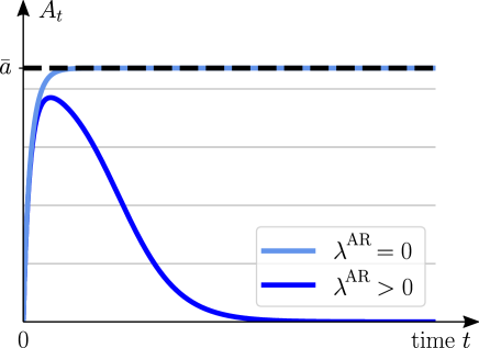
Figure 6: Evolution of $A_{t}$ for an active agent who starts out as susceptible.

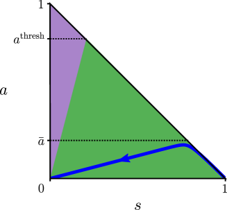
Figure 7: The trajectory of Fig. 6 (for $\lambda^{\text{\tiny AR}}>0$) depicted on the simplex. An agent’s optimal decision is to remain active, unless it starts to show symptoms.

The answer to the second question is as follows:

1. Even though an individual agent’s conditional probability $A_{t}$ is small at any time $t<\tau$, the law of large numbers (LLN) dictates that in a large population with $N$ agents, ${\sf E}(A_{t})$ fraction of agents are asymptomatic with high probability.

2. The basic reproduction number $R_{o}$ (pronounced $R$ nought) is defined as $\frac{T^{\text{r}}}{T^{\text{c}}}$ where $T^{\text{r}}$ is the average time until removal (in our settings, either showing symptoms $x=\textbf{\emph{i}}$ or recovery $x=\textbf{\emph{r}}$) and $T^{\text{c}}$ is the average time between infectious contacts. For our model, this ratio is $\frac{\lambda^{\text{\tiny SA}}}{\lambda^{\text{\tiny AI}}+\lambda^{\text{\tiny AR}}}=R_{o}$.

3. If $R_{o}>1$ then for small values of $\bar{\beta}$, optimal actions of individual agents (to remain active) still causes an epidemic.

The above is an example of rational irrationality where rational choices of individual agents lead to irrational outcomes for the population [18, 19]. It is notable that the irrationality here is entirely a consequence of the lack of information (with full information, asymptomatic agents isolate).

A limitation of these arguments is that the analysis is rather qualitative and moreover relies on the assumption of a given stationarity $\beta_{t}\equiv\bar{\beta}$. Indeed, this is not necessarily true in the case of an epidemic: The process $\beta$ is non-stationary and also a result of the individual actions of many agents. This motivates the need for a more refined analysis based on a mean-field game model as described next.

V Mean-field game model

In this section, we consider a population of heterogeneous agents. As already noted, $\rho_{t}(x,u;\theta)$ is the joint distribution of the state-action pair $(X_{t},U_{t})$ at time $t$, conditioned on the attribute $\theta$. The marginal pmf $\rho_{t}(x;\theta)$ evolves according to the mean-field equations:

$$\frac{\,\mathrm{d}\rho_{t}}{\,\mathrm{d}t}(\textbf{\emph{s}};\theta) =-\lambda^{\text{\tiny SA}}\beta_{t}\int_{0}^{1}u\rho_{t}(\textbf{\emph{s}},u;\theta)\,\mathrm{d}u-\eta\rho_{t}(\textbf{\emph{s}};\theta)$$ (6a)

$$\frac{\,\mathrm{d}\rho_{t}}{\,\mathrm{d}t}(x;\theta) =({\cal A}^{\dagger}\rho_{t})(x;\theta),\quad x\in\{\textbf{\emph{i}},\textbf{\emph{a}},\textbf{\emph{r}},\textbf{\emph{d}}\}$$ (6b)

from a given initial condition $\rho_{0}(x;\theta)$; ${\cal A}^{\dagger}$ is the adjoint of the generator ${\cal A}$ of the Markov process $X$.

Each agent in the population chooses its control according to the optimal control law $\psi_{t}(\cdot;\theta)$ obtained from solving the HJB equation (the notation denotes the dependence on the attribute $\theta$). In the two cases,

$$\text{(fully obsvd.)}\qquad U_{t} =\psi_{t}(X_{t};\theta)$$

$$\text{(part. obsvd.)}\qquad U_{t} =\psi_{t}(\pi_{t};\theta)\$$

where $\pi_{t}={\sf P}(X_{t}\mid{\cal Y}_{t})$ is the belief state; the use of the common notation $\psi_{t}(\cdot;\theta)$ should not cause any confusion because the two cases are treated in separate subsections.

The following operators are of interest (see Sec. II-C for definition of function space ${\cal M}$ and ${\cal U}$):

1. The operator $\Psi:{\cal M}\to{\cal U}$, defined as

   $$\Psi(\beta)=\mathop{\text{\rm arg\,min}}_{U\in{\cal U}}{\sf J}(U;\beta)$$

2. The operator $\Xi:{\cal U}\to{\cal M}$, defined according to (6) where $\beta$ is obtained using (1).

Assuming that the two operators are well-defined, we have:

Definition 1

A mean-field equilibrium (MFE) is a fixed point $\beta$ such that $\Xi(\Psi(\beta))=(\beta)$.

V-A Fully Observed Case

For the fully observed problem, a complete characterization of the MFG equilibrium is described in the following proposition. The result is a minor extension of a similar result appearing in our prior paper [1] (for $\lambda^{\text{\tiny AR}}$ and $\eta=0$) and therefore its proof is omitted.

Proposition 6

The unique mean-field equilibrium is

$$\beta_{t}=0\quad\forall\;\;t\geq 0$$

This result represents a mathematical expression of the thought experiment described in Sec. I. Its main utility is to set up the problem whereby the effects of some of the underlying assumptions – perfect rationality and perfect information – can be investigated. As with the preceding sections, the main focus of the MFG modeling is in the partially observed settings, which is the subject of the following subsection.

V-B Partially Observed Case

Consider the space of probability distributions on the belief space ${\cal P}^{1}\cup{\cal P}^{2}$. The random vector $(S_{t},A_{t})$ is well-defined on the set $[t<\tau]$, and we denote by $p_{t}(s,a)$ its density for $0\leq s\leq 1$, $s+a\leq 1$:

$${\sf P}([s<S_{t}<s+\,\mathrm{d}s]\cap[a<A_{t}<a+\,\mathrm{d}a]\cap[t<\tau])$$

$$=p_{t}(s,a)\,\mathrm{d}a\,\mathrm{d}s,\quad t\geq 0$$

Assumption 1

The density $p_{t}(s,1-s)=p_{t}(s,0)=0$ for all $t\geq 0$, $s\in[0,1]$.

Under Assumption 1 that an agent uses the optimal control $U_{t}=U_{t}^{\text{opt}}=\psi_{t}(S_{t},A_{t})$ for $0\leq t<\tau$, the density process $\{p_{t}(s,a)\in[0,\infty):0\leq s\leq 1,s+a\leq 1,t\geq 0\}$ solves the FPK equation whose derivation, along with the expressions for $f_{\textbf{\emph{s}}}(s,a,t)$ and $f_{\textbf{\emph{a}}}(s,a,t)$, appears in Appendix -E:

$$\frac{\partial p_{t}}{\partial t}(s,a) =-\frac{\partial}{\partial s}\big{(}f_{\textbf{\emph{s}}}(s,a,t)p_{t}(s,a)\big{)}$$

$$-\frac{\partial}{\partial a}\big{(}f_{\textbf{\emph{a}}}(s,a,t)p_{t}(s,a)\big{)}-a\lambda^{\text{\tiny AI}}p_{t}(s,a)$$ (7)

where $p_{0}(s,a)$ is the initial density (assumed given). By using the tower property,

$$\rho_{t}(\textbf{\emph{a}}) ={\sf P}([X_{t}=\textbf{\emph{a}}])$$

$$={\sf E}(\pi_{t}(\textbf{\emph{a}}))={\sf E}(A_{t}1_{[t<\tau]})=\int_{0}^{1}\int_{0}^{1-s}ap_{t}(s,a)\,\mathrm{d}a\,\mathrm{d}s$$

and therefore we have

$$\frac{\,\mathrm{d}\rho_{t}}{\,\mathrm{d}t}(\textbf{\emph{i}}) =\lambda^{\text{\tiny AI}}\int_{0}^{1}\int_{0}^{1-s}ap_{t}(s,a)\,\mathrm{d}a\,\mathrm{d}s-(\lambda^{\text{\tiny ID}}+\lambda^{\text{\tiny IR}})\rho_{t}(\textbf{\emph{i}})$$ (8a)

$$\frac{\,\mathrm{d}\rho_{t}}{\,\mathrm{d}t}(x) =({\cal A}^{\dagger}\rho_{t})(x),\quad x\in\{\textbf{\emph{r}},\textbf{\emph{d}}\}$$ (8b)

where expression for ${\cal A}^{\dagger}$ is obtained from the transition graph.

With a heterogeneous population, the notation $p_{t}(s,a;\theta)$ is used to denote the density conditioned on the attribute $\theta$. The mean-field process is then consistently obtained as

$$\beta_{t}=\sum_{\theta}{\sf p}(\theta) \int_{0}^{1}\int_{0}^{1-s}a\psi_{t}(s,a;\theta)p_{t}(s,a;\theta)\,\mathrm{d}a\,\mathrm{d}s$$ (9)

This completes the derivation of the system of equations for the partially observed MFG: Eq. (7)-(8) is the forward FPK equation. Eq. (4) is the backward HJB equation. Eq. (9) defines the consistency relationship that links the two equations. Its solution is an MFE (satisfies Defn. 1).

The thrust of the ongoing work is to obtain numerical solutions of the MFG equations and use it to explain differences between the data from the omicron and delta waves.

-C Proof of Proposition 3

With $\beta_{t}=\bar{\beta}$, the HJB equation for $v_{t}(\textbf{\emph{s}})$ is

$$-\frac{\,\mathrm{d}v_{t}}{\,\mathrm{d}t}(\textbf{\emph{s}}) +(\gamma+\eta)v_{t}(\textbf{\emph{s}})$$

$$=\eta\bar{\phi}(\textbf{\emph{a}})+\min_{u\in[0,1]}\left(\lambda^{\text{\tiny SA}}\bar{\beta}\left(\bar{\phi}(\textbf{\emph{a}})-v_{t}(\textbf{\emph{s}})\right)-\alpha\right)u$$

We investigate its stationary solutions $v_{t}(\textbf{\emph{s}})=\bar{\phi}(\textbf{\emph{s}})$ in which case the stationary HJB equation is

$$(\gamma+\eta)\bar{\phi}(\textbf{\emph{s}}) =\eta\bar{\phi}(\textbf{\emph{a}})$$

$$+\min_{u\in[0,1]}\underbrace{\left(\lambda^{\text{\tiny SA}}\bar{\beta}\left(\bar{\phi}(\textbf{\emph{a}})-\bar{\phi}(\textbf{\emph{s}})\right)-\alpha\right)}_{=:M}u$$ (10)

We have the following two cases:

• If $\bar{\beta}<\frac{\alpha}{\lambda^{\text{\tiny SA}}\bar{\phi}(\textbf{\emph{a}})}\left(1+\frac{\eta}{\gamma}\right)$, then $\bar{\phi}(\textbf{\emph{s}})=\frac{(\lambda^{\text{\tiny SA}}\bar{\beta}+\eta)\bar{\phi}(\textbf{\emph{a}})-\alpha}{\lambda^{\text{\tiny SA}}\bar{\beta}+\gamma+\eta}$ solves the HJB equation with the minimizing choice of $u=1$, because

  $$M=\lambda^{\text{\tiny SA}}\bar{\beta}\left(\frac{\gamma\bar{\phi}(\textbf{\emph{a}})+\alpha}{\lambda^{\text{\tiny SA}}\bar{\beta}+\gamma+\eta}\right)-\alpha<0$$

  $$\iff \lambda^{\text{\tiny SA}}\bar{\beta}\alpha+\gamma\alpha+\eta\alpha>\lambda^{\text{\tiny SA}}\bar{\beta}\gamma\bar{\phi}(\textbf{\emph{a}})+\lambda^{\text{\tiny SA}}\bar{\beta}\alpha$$

  $$\iff \bar{\beta}<\frac{\alpha}{\lambda^{\text{\tiny SA}}\bar{\phi}(\textbf{\emph{a}})}\left(1+\frac{\eta}{\gamma}\right)$$

• If $\bar{\beta}>\frac{\alpha}{\lambda^{\text{\tiny SA}}\bar{\phi}(\textbf{\emph{a}})}\left(1+\frac{\eta}{\gamma}\right)$, then $\bar{\phi}(\textbf{\emph{s}})=\frac{\eta}{\gamma+\eta}\bar{\phi}(\textbf{\emph{a}})$ solves the HJB equation with the minimizing choice of $u=0$, because

  $$M=\frac{\lambda^{\text{\tiny SA}}\bar{\beta}\gamma\bar{\phi}(\textbf{\emph{a}})}{\gamma+\eta}-\alpha>0$$

-D Proof of Proposition 5

Because $A_{0}=0$, and the solution is continuous as a function of time $t$, it suffices to show that

$$A_{t}=\frac{\lambda^{\text{\tiny SA}}\bar{\beta}+\eta}{\lambda^{\text{\tiny AI}}}\implies\frac{\,\mathrm{d}A_{t}}{\,\mathrm{d}t}<0$$

Setting $A_{t}=\frac{\lambda^{\text{\tiny SA}}\bar{\beta}+\eta}{\lambda^{\text{\tiny AI}}}$ on the righthand side of (3),

$$\frac{\,\mathrm{d}A_{t}}{\,\mathrm{d}t}=(\lambda^{\text{\tiny SA}}\bar{\beta}+\eta)\left(S_{t}-1+\frac{\lambda^{\text{\tiny SA}}\bar{\beta}+\eta-\lambda^{\text{\tiny AR}}}{\lambda^{\text{\tiny AI}}}\right)$$

The desired conclusion follows because $S_{t}+A_{t}\leq 1$ and therefore $S_{t}-1+\frac{\lambda^{\text{\tiny SA}}\bar{\beta}+\eta}{\lambda^{\text{\tiny AI}}}\leq 0$ if $A_{t}=\frac{\lambda^{\text{\tiny SA}}\bar{\beta}+\eta}{\lambda^{\text{\tiny AI}}}$.

-E Derivations

Let ${\cal P}:={\cal P}^{1}\cup{\cal P}^{2}$. The belief process $\pi:=\{\pi_{t}\in{\cal P}:t\geq 0\}$ is a Markov process [20, Theorem 1.7]. The HJB equations and FPK equations are easily derived once we obtain the infinitesimal generator of the process.

Infinitesimal generator: Consider a smooth test function $v:{\cal P}\to\mathbb{R}$. Let $\mu\in{\cal P}$. The infinitesimal generator (for the general time-inhomogeneous case) is

$$({\cal A}_{t}^{u}v)(\mu)=\lim_{\delta t\downarrow 0}\frac{{\sf E}(v(\pi_{t+\delta t})|\pi_{t}=\mu)-v(\mu)}{\delta t}$$

There are two cases to consider:

$\bullet$ If $\mu\in{\cal P}^{2}$, upon identifying the measures $\{\delta_{\textbf{\emph{i}}},\delta_{\textbf{\emph{r}}},\delta_{\textbf{\emph{d}}}\}$ with the states $\{\textbf{\emph{i}},\textbf{\emph{r}},\textbf{\emph{d}}\}$, the generator is the same as the generator for the Markov process.

$\bullet$ If $\mu\in{\cal P}^{1}\setminus\{\delta_{\textbf{\emph{r}}}\}$, then using the coordinates $(s,a)$ for ${\cal P}^{1}$, $\mu=[s,a,0,1-s-a,0]$ for $a\in[0,1]$. With $\pi_{t}=\mu$, in the asymptotic limit as $\delta t\to 0$,

$$\pi_{t+\delta t}=\begin{cases}\mu+e_{\textbf{\emph{s}}}f_{\textbf{\emph{s}}}(s,a,t)\delta t\\ +e_{\textbf{\emph{a}}}f_{\textbf{\emph{a}}}(s,a,t)\delta t+o(\delta t)&\text{w.p.}\;\;(1-a\lambda^{\text{\tiny AI}}\delta t)+o(\delta t)\\ \delta_{\textbf{\emph{i}}}&\text{w.p.}\;\;a\lambda^{\text{\tiny AI}}\delta t+o(\delta t)\end{cases}$$

where

$$f_{\textbf{\emph{s}}}(s,a,t) =\left(-\lambda^{\text{\tiny SA}}\beta_{t}u-\eta+a\lambda^{\text{\tiny AI}}\right)s$$

$$f_{\textbf{\emph{a}}}(s,a,t) =\left(\lambda^{\text{\tiny SA}}\beta_{t}u+\eta\right)s+a\left(-\lambda^{\text{\tiny AI}}-\lambda^{\text{\tiny AR}}+\lambda^{\text{\tiny AI}}a\right)$$

and $e_{\textbf{\emph{s}}}=[1,0,0,-1,0]$, $e_{\textbf{\emph{a}}}=[0,1,0,-1,0]$. Denoting $v(\mu)=\phi(s,a)$, the generator is then easily calculated to be

$$({\cal A}_{t}^{u}v)(\mu) =f_{\textbf{\emph{s}}}(s,a,t)\frac{\partial\phi}{\partial s}(s,a)+f_{\textbf{\emph{a}}}(s,a,t)\frac{\partial\phi}{\partial a}(s,a)$$

$$+a\lambda^{\text{\tiny AI}}(v(\delta_{\textbf{\emph{i}}})-\phi(s,a))$$

where the superscript $u$ denotes the fact that $f_{\textbf{\emph{s}}}(s,a,t)$, $f_{\textbf{\emph{a}}}(s,a,t)$, and therefore also the generator, depends also upon $u$. The subscript $t$ denotes the fact that the generator is for a time-inhomogeneous Markov process (because $\beta$ may depend upon time).

Derivation of the HJB equation: The HJB equation (See Sec.III.7 of [21]) is

$$-\frac{\partial v_{t}}{\partial t}(\mu)+\gamma v_{t}(\mu)=\min_{u\in[0,1]}\left({\cal A}_{t}^{u}v_{t}(\mu)+\mu(c(\cdot,u;\alpha))\right)$$

In order to calculate $\mu\big{(}c(\cdot,u;\alpha)\big{)}$, we need to assume a running cost for state r. If we assume $c(\textbf{\emph{r}},\cdot;\cdot)=\gamma\bar{\phi}(\textbf{\emph{r}})$, then we get

$$\int_{0}^{\infty}c(\textbf{\emph{r}},\cdot;\cdot)e^{-\gamma t}dt=\bar{\phi}(\textbf{\emph{r}})$$

as desired. Let

$$\mathcal{L}\phi:=(1-s-a)\gamma\bar{\phi}(\textbf{\emph{r}})+a\lambda^{\text{\tiny AI}}\left(\bar{\phi}(\textbf{\emph{i}})-\phi\right)$$

$$+(a\lambda^{\text{\tiny AI}}-\eta)s\frac{\partial\phi}{\partial s}+\left(\eta s+a(a\lambda^{\text{\tiny AI}}-\lambda^{\text{\tiny AI}}-\lambda^{\text{\tiny AR}})\right)\frac{\partial\phi}{\partial a}$$

$${\cal M}_{t}(s,a):=a-(s+a)\alpha+\lambda^{\text{\tiny SA}}\beta_{t}s\left(\frac{\partial\phi_{t}}{\partial a}-\frac{\partial\phi_{t}}{\partial s}\right)$$

Thus for $\mu=[s,a,0,1-s-a,0]$ and $v_{t}(\mu)=\phi_{t}(s,a)$, the HJB equation (4) is obtained because

$$\mu\big{(}c(\cdot,u;\alpha)\big{)} =(1-s-a)\gamma\bar{\phi}(\textbf{\emph{r}})+s(-\alpha u)+a(1-\alpha)u$$

$$=(1-s-a)\gamma\bar{\phi}(\textbf{\emph{r}})+(a-(s+a)\alpha)u$$

The boundary conditions (5) follow from the observation that

$$\phi_{t}(s,a)$$

$$=s\min_{U\in L_{\mathcal{F}}^{2}}{\sf E}\bigg{(}\int_{t}^{T}e^{-\gamma s}c(X_{s},U_{s};\alpha)ds+e^{-\gamma T}\phi(X_{T})$$

$$\mid X_{t}=\textbf{\emph{s}}\bigg{)}+a\bar{\phi}(\textbf{\emph{a}})+(1-s-a)\bar{\phi}(\textbf{\emph{r}})$$

Derivation of the FPK equation: We derive the adjoint of the generator ${\cal A}^{u}$ where dependence on $t$ is suppressed for notational ease. Let $\rho$ be a measure on ${\cal P}$. On ${\cal P}^{1}$, $\rho$ has density $p(s,a)$. Consider $\rho({\cal A}^{u}v)=\int{\cal A}^{u}v(\mu)\rho(\,\mathrm{d}\mu)=$

$$\int_{0}^{1}\int_{0}^{1-s}p(s,a)\bigg{[}f_{\textbf{\emph{s}}}(s,a)\frac{\partial\phi}{\partial s}+f_{\textbf{\emph{a}}}(s,a)\frac{\partial\phi}{\partial a}$$

$$+a\lambda^{\text{\tiny AI}}\big{(}v(\delta_{\textbf{\emph{i}}})-\phi(s,a)\big{)}\bigg{]}\,\mathrm{d}a\,\mathrm{d}s-\rho(\delta_{\textbf{\emph{i}}})(\lambda^{\text{\tiny IR}}+\lambda^{\text{\tiny ID}})v(\delta_{\textbf{\emph{i}}})$$

$$+\rho(\delta_{\textbf{\emph{r}}})\lambda^{\text{\tiny IR}}v(\delta_{\textbf{\emph{r}}})+\rho(\delta_{\textbf{\emph{d}}})\lambda^{\text{\tiny ID}}v(\delta_{\textbf{\emph{d}}})$$ (11)

First note that

$$\int_{0}^{1-a}p(s,a)f_{\textbf{\emph{s}}}(s,a)\frac{\partial\phi}{\partial s}\,\mathrm{d}s=p(s,a)f_{\textbf{\emph{s}}}(s,a)\phi(s,a)|_{s=0}^{s=1-a}$$

$$-\int_{0}^{1-a}\phi(s,a)\frac{\partial}{\partial s}\big{(}p(s,a)f_{\textbf{\emph{s}}}(s,a)\big{)}\,\mathrm{d}s$$

where boundary terms vanish because $f_{\textbf{\emph{s}}}(0,a)=0$ and $p(1-a,a)=0$ (Assumption 1). One can also write

$$\int_{0}^{1-s}p(s,a)f_{\textbf{\emph{a}}}(s,a)\frac{\partial\phi}{\partial a}\,\mathrm{d}a=p(s,a)f_{\textbf{\emph{a}}}(s,a)\phi(s,a)|_{a=0}^{a=1-s}$$

$$-\int_{0}^{1-s}\phi(s,a)\frac{\partial}{\partial a}\big{(}p(s,a)f_{\textbf{\emph{a}}}(s,a)\big{)}\,\mathrm{d}a$$

where boundary terms vanish because $p(s,1-s)=p(s,0)=0$ (Assumption 1). Using these two results, one can rewrite the righthand side of (11) as

$$-\int_{0}^{1}\int_{0}^{1-s}\phi(s,a)\bigg{[}\frac{\partial}{\partial s}\big{(}p(s,a)f_{\textbf{\emph{s}}}(s,a)\big{)}+\frac{\partial}{\partial a}\big{(}p(s,a)f_{\textbf{\emph{a}}}(s,a)\big{)}$$

$$+a\lambda^{\text{\tiny AI}}p(s,a)\bigg{]}\,\mathrm{d}a\,\mathrm{d}s+v(\delta_{\textbf{\emph{r}}})\lambda^{\text{\tiny IR}}\rho(\delta_{\textbf{\emph{r}}})+v(\delta_{\textbf{\emph{d}}})\lambda^{\text{\tiny ID}}\rho(\delta_{\textbf{\emph{d}}})$$

$$+v(\delta_{\textbf{\emph{i}}})\left(\int_{0}^{1}\int_{0}^{1-s}a\lambda^{\text{\tiny AI}}p(s,a)\,\mathrm{d}a\,\mathrm{d}s-(\lambda^{\text{\tiny IR}}+\lambda^{\text{\tiny ID}})\rho(\delta_{\textbf{\emph{i}}})\right)$$

-F Numerical Algorithm

The HJB equation (4) is numerically solved using the method of lines. In this method, the spatial coordinate $(s,a)\in D$ is discretized over a finite grid. The partial derivatives $\partial\phi_{t}/\partial s$ and $\partial\phi_{t}/\partial a$ are approximated using a finite difference approximation at each point on the grid. The time variable $t$ is treated as a continuous variable and after spatial discretization, the resulting ordinary differential equations are numerically integrated (backward in time) using a standard numerical procedure. For this purpose, a sufficiently large terminal time $T$ is chosen with the following terminal condition:

$$\phi_{T}(s,a)=\begin{cases}a\bar{\phi}(\textbf{\emph{a}})+(1-a)\bar{\phi}(\textbf{\emph{r}})&a\leq\frac{1-s}{2}\\ \phi_{T}(s,1-s-a)\\ +(2a+s-1)\left(\bar{\phi}(\textbf{\emph{a}})-\bar{\phi}(\textbf{\emph{r}})\right)&a>\frac{1-s}{2}\end{cases}$$

The algorithm was used to compute the stationary solutions depicted in Fig. 5.

References

- [1] S. Y. Olmez, S. Aggarwal, J. W. Kim, E. Miehling, T. Başar, M. West, and P. G. Mehta, “Modeling presymptomatic spread in epidemics via mean-field games,” arXiv preprint arXiv:2111.10422, 2021.
- [2] L. Rivett, S. Sridhar, D. Sparkes, M. Routledge, N. K. Jones, S. Forrest, J. Young, J. Pereira-Dias, W. L. Hamilton, M. Ferris et al., “Screening of healthcare workers for SARS-CoV-2 highlights the role of asymptomatic carriage in COVID-19 transmission,” Elife, vol. 9, p. e58728, 2020.
- [3] D. C. Buitrago-Garcia, D. Egli-Gany, M. J. Counotte, S. Hossmann, H. Imeri, G. Salanti, and N. Low, “The role of asymptomatic SARS-CoV-2 infections: rapid living systematic review and meta-analysis,” MedRxiv, 2020.
- [4] J. K. Bender, M. Brandl, M. Höhle, U. Buchholz, and N. Zeitlmann, “Analysis of asymptomatic and presymptomatic transmission in SARS-CoV-2 outbreak, Germany, 2020,” Emerging infectious diseases, vol. 27, no. 4, p. 1159, 2021.
- [5] W. E. Wei, Z. Li, C. J. Chiew, S. E. Yong, M. P. Toh, and V. J. Lee, “Presymptomatic transmission of SARS-CoV-2—Singapore, january 23–march 16, 2020,” Morbidity and Mortality Weekly Report, vol. 69, no. 14, p. 411, 2020.
- [6] R. Elie, E. Hubert, and G. Turinici, “Contact rate epidemic control of COVID-19: an equilibrium view,” Mathematical Modelling of Natural Phenomena, vol. 15, p. 35, 2020.
- [7] A. Aurell, R. Carmona, G. Dayanikli, and M. Lauriere, “Optimal incentives to mitigate epidemics: a Stackelberg mean field game approach,” arXiv preprint arXiv:2011.03105, 2020.
- [8] ——, “Finite state graphon games with applications to epidemics,” arXiv preprint arXiv:2106.07859, 2021.
- [9] E. Hubert, T. Mastrolia, D. Possamaï, and X. Warin, “Incentives, lockdown, and testing: from thucydides’s analysis to the covid-19 pandemic,” arXiv preprint arXiv:2009.00484, 2020.
- [10] W. Lee, S. Liu, H. Tembine, W. Li, and S. Osher, “Controlling propagation of epidemics via mean-field control,” arXiv preprint arXiv:2006.01249, 2020.
- [11] S. Cho, “Mean-field game analysis of SIR model with social distancing,” arXiv preprint arXiv:2005.06758, 2020.
- [12] J. Doncel, N. Gast, and B. Gaujal, “A mean field game analysis of SIR dynamics with vaccination,” Probability in the Engineering and Informational Sciences, pp. 1–18, 2020.
- [13] H. Tembine, “COVID-19: Data-driven mean-field-type game perspective,” Games, vol. 11, no. 4, p. 51, 2020.
- [14] N. Saldi, T. Başar, and M. Raginsky, “Partially-observed discrete-time risk-sensitive mean-field games,” in 2019 IEEE 58th Conference on Decision and Control (CDC). IEEE, 2019, pp. 317–322.
- [15] N. Saldi, T. Başar, and M. Raginsky, “Approximate nash equilibria in partially observed stochastic games with mean-field interactions,” Mathematics of Operations Research, vol. 44, no. 3, pp. 1006–1033, 2019. [Online]. Available: https://doi.org/10.1287/moor.2018.0957
- [16] F. Confortola and M. Fuhrman, “Filtering of continuous-time markov chains with noise-free observation and applications,” Stochastics An International Journal of Probability and Stochastic Processes, vol. 85, no. 2, pp. 216–251, 2013.
- [17] S. Cobey, J. Bloom, T. Starr, and N. Lash, “We study virus evolution. here’s where we think the coronavirus is going.” New York Times, 2022. [Online]. Available: https://www.nytimes.com/interactive/2022/03/28/opinion/coronavirus-mutation-future.html
- [18] J. Cassidy, “Rational irrationality: The real reason that capitalism is so crash-prone,” Oct. 5th 2009.
- [19] H. Yin, P. G. Mehta, S. P. Meyn, and U. V. Shanbhag, “Synchronization of oscillators is a game,” in IEEE Transactions on Automatic Control, vol. 57, no. 4, April 2012, pp. 920–935.
- [20] J. Xiong, An Introduction to Stochastic Filtering Theory. Oxford University Press, 2008.
- [21] W. H. Fleming and H. M. Soner, Controlled Markov Processes and Viscosity Solutions, 2nd ed., ser. Stochastic Modelling and Applied Probability ; 25. New York: Springer-Verlag, 2006.