Optimizing Sensing Matrices for Spherical Near-Field Antenna Measurements

Abstract

In this article, we address the problem of reducing the number of required samples for Spherical Near-Field Antenna Measurements (SNF) by using Compressed Sensing (CS). A condition to ensure the numerical performance of sparse recovery algorithms is the design of a sensing matrix with low mutual coherence. Without fixing any part of the sampling pattern, we propose sampling points that minimize the mutual coherence of the respective sensing matrix by using augmented Lagrangian method. Numerical experiments show that the proposed sampling scheme yields a higher recovery success in terms of phase transition diagram when compared to other known sampling patterns, such as the spiral and Hammersley sampling schemes. Furthermore, we also demonstrate that the application of CS with an optimized sensing matrix requires fewer samples than classical approaches to reconstruct the Spherical Mode Coefficients (SMCs) and far-field pattern.

1 Introduction

Compared to other acquisition methods to characterize an antenna’s radiation pattern, Spherical Near-Field Antenna Measurements (SNF) are a convenient and cost-effective way of ascertaining the radiation characteristics of an Antenna Under Test (AUT). Additionally, since the measurement conditions in smaller ranges are easier to control and the obtained results undergo a mathematical transformation that forces them to be physical, their accuracy is higher than for other methods, going as far as being considered the most accurate antenna measurement method [1]. While the biggest challenge of this method may seem the implementation of the mathematical Near-Field to Far-Field Transformation (NFFFT), one of the most challenging problems is, in fact, the choice of the measurement’s sampling strategy. The chosen sampling strategy must ensure that the information of interest is included from an information-theory standpoint and must, also, enable a convenient NFFFT. Classically, the Nyquist theorem is applied to the equator of the AUT to derive the angular resolution of the sampling scheme, and this angular step is replicated for both classical sampling axes – azimuth and elevation. The resulting sampling scheme is often called equiangular, and its main drawback is that, considering an information-theory perspective, it results in an equation system with more than double the number of equations, i.e., samples, than variables, i.e., Spherical Mode Coefficients (SMCs) [2]. As a consequence, one of the strongest objections to this method is its long acquisition time.

Vibrant research activity has been done to overcome this issue. For instance, the authors of [3] use a spiral scanning approach to reduce the density of the samples near the spherical poles, which is a direct implication of using an equiangular sampling. Along the same lines, the strategy to reduce sampling points on azimuthal axes has been proposed in [4]. In addition, the authors also provide an aliasing error estimator to address the aliasing problem that appears naturally when reducing the samples on these axes. Instead of changing the sampling mechanism, the authors in [5] propose a new NFFFT method with downsampling property during the acquisition process. A similar approach has been developed in [6] by using non-uniform Fourier transform to accommodate non-equiangular near-field acquisitions, in contrast to the original transformation method that employs conventional Fourier transforms with equiangular sampling points [2].

Another strategy to address the long acquisition time is by employing Compressed Sensing (CS), which models the acquisition process as a linear system of equations and applies sparse recovery algorithms, e.g., Basis Pursuit (BP), to solve an underdetermined system of equations. This approach stems from the fact that, in most observations, the SMCs are sparse or compressible, meaning that only a small amount of coefficients contains high power, as discussed in [7, 8, 9, 10].

In CS theory, if the sensing matrix satisfies certain conditions, for example Restricted Isometry Property (RIP), then it is guaranteed that sparse-recovery algorithms such as BP yield a recovery error bounded by the measurement noise and model mismatch [11, 12]. Random subgaussian matrices are known to satisfy RIP with high probability and thereby have recovery guarantees. This is a considerable roadblock for the practical application of CS in SNF, since random sampling schemes cannot guarantee in any way that the mechanical movements required to scan them indeed reduce the acquisition time when compared to equiangular sampling schemes [10]. Besides, it has been proven in [13, 14] that verifying RIP property for a given deterministic sensing matrices is an NP-hard problem. Therefore, the RIP condition does not provide an adequate guideline for deterministic sensing matrix design. Apart from RIP, another approach to guaranteeing the recovery of sparse signals is the designing low-coherence sensing matrices. Despite providing a weaker reconstruction guarantee when compared to RIP, the computation of the mutual coherence is computationally tractable, since it only consists of a dot product of adjacent columns of a sensing matrix. For this reason, designing a low-coherence sensing matrix is preferred in most applications, such as electromagnetic imaging [15] and radar [16]. In the mentioned examples, the implementation of CS has been conducted by using the mutual coherence as a metric to numerically assess whether that the reconstruction algorithms yield a correct solution with fewer measurement points.

The challenge to construct a low-coherence sensing matrix in SNF is that the multipole expansion of electromagnetic fields and antenna measurements requires specific functions, called spherical harmonics and Wigner D-functions, respectively. These functions follow certain polynomial structures, and their optimization is challenging. In this work, we present a method to optimize sensing matrices for SNF in terms of their mutual coherence.

1.1 Related Works

The construction of a sensing matrix from Wigner D-functions and their specific case, namely spherical harmonics, in the area of CS has been discussed in [17, 18, 19, 20]. However, these works emphasize more on the design of RIP sensing matrices with random sampling and theoretical recovery guarantee using BP. Although we have a bound on the minimum required number of measurements, in practice, this bound seems pessimistic, as discussed in [21], since the BP algorithm is still able to numerically reconstruct the sparse coefficients even with fewer samples distributed in a spiral pattern. This investigation leads to the question of whether other types of deterministic sampling points can be designed to yield a higher recovery success, even if just numerically.

In [22, 20], the authors aim to show that a specific sampling pattern, e.g., the equiangular sampling scheme, leads to the construction of a high coherence sensing matrix and fails to reconstruct the sparse signal which, in turn, excludes a construction of sensing matrices based on such a sampling strategy for CS applications. Additionally, the authors derive an achievable coherence bound that can be used to design a low coherence sensing matrix for SNF setting [23]. However, the drawback to this approach is that, while fixing a specific pattern on the elevation axes is advantageous for mechanical scanning systems, some degree of freedoms are lost in comparison to a full optimization on the whole spherical surface.

1.2 Summary of Contributions

The main contributions of our paper are as follows:

• We propose a gradient-based method by smoothing the objective function to minimize the coherence in terms of $\ell_{p}$-norm. Thereby, we only have to set a large enough $p$ to approximate the maximum norm.

• Besides, we also propose an Augmented Lagrangian Method (ALM)-based proximal method. This approach provides an efficient strategy to decompose the original problem into subproblems. By using the proximal for the $\ell_{\infty}$-norm, we do not have to directly compute gradient or sub-gradient $\ell_{\infty}$-norm.

• We also provide numerical simulations to evaluate the coherence of a sensing matrix from both algorithms and compare them to the coherence of a sensing matrix constructed from well-known sampling patterns. We numerically show that our proposed sampling scheme outperform other well-known sampling patterns and deliver results similar to their random counterparts.

• At last, we apply optimized sensing matrices for experimental data and perform sparse SMCs reconstruction, and use these to reconstruct the far-field pattern. Numerically, we show that by using optimized sensing matrices for CS it is possible to reduce the number of samples to reconstruct an AUT’s far-field pattern.

2 Compressed Sensing

In most signal acquisition processes, it is enough to model the measurement processes with a linear system as follows:

$$\mathbf{y}=\mathbf{A}\mathbf{x},$$ (1)

where $\mathbf{A}\in\mathbb{C}^{K\times L}$ is the sensing matrix. CS provides a framework to recover the sparse structure of $\mathbf{x}$ from a smaller dimension of the acquired signal $\mathbf{y}\in\mathbb{C}^{K}$, i.e., $K<L$. Basis Pursuit (BP) is one of the well-known algorithms to estimate the sparse vector $\mathbf{x}$ by solving the following optimization problem

$$\underset{\mathbf{\hat{x}}}{\text{minimize}} \left\|\mathbf{\hat{x}}\right\|_{1} \mathbf{y}=\mathbf{A}\mathbf{\hat{x}}.$$ subject to (P1)

Theoretically speaking, it is necessary to have a fundamental limit on the required number of measurements $K$ to ensure the unique reconstruction of sparse vector $\mathbf{x}$, meaning that the estimated vector $\mathbf{\hat{x}}$ and the ground truth vector $\mathbf{x}$ are close enough in terms of small numerical differences. Low coherence of the matrix $\mathbf{A}$ are well-known properties to provide a sufficient condition and robustness of the reconstruction of sparse vector $\mathbf{x}$ [24, 11, 12].

For a matrix $\mathbf{A}=[\IfSubStr{abcdefghijklmnopqrstuvwxyzABCDEFGHIJKLMNOPQRST123456789}{a}{\mathbf{{a}}}{\boldsymbol{{a}}}_{1}\dots\IfSubStr{abcdefghijklmnopqrstuvwxyzABCDEFGHIJKLMNOPQRST123456789}{a}{\mathbf{{a}}}{\boldsymbol{{a}}}_{L}]\in\mathbb{C}^{K\times L}$, the mutual coherence is defined as

$$\mu(\mathbf{A}):=\max_{1\leq i<j\leq L}\frac{\left|\langle\IfSubStr{abcdefghijklmnopqrstuvwxyzABCDEFGHIJKLMNOPQRST123456789}{a}{\mathbf{{a}}}{\boldsymbol{{a}}}_{i},\IfSubStr{abcdefghijklmnopqrstuvwxyzABCDEFGHIJKLMNOPQRST123456789}{a}{\mathbf{{a}}}{\boldsymbol{{a}}}_{j}\rangle\right|}{\left\|\IfSubStr{abcdefghijklmnopqrstuvwxyzABCDEFGHIJKLMNOPQRST123456789}{a}{\mathbf{{a}}}{\boldsymbol{{a}}}_{i}\right\|_{2}\left\|\IfSubStr{abcdefghijklmnopqrstuvwxyzABCDEFGHIJKLMNOPQRST123456789}{a}{\mathbf{{a}}}{\boldsymbol{{a}}}_{j}\right\|_{2}},$$

where the lowest coherence we can get is lower bounded by the Welch bound [25], which is given as

$$\mu(\mathbf{A})\geq\sqrt{\frac{L-K}{K(L-1)}}.$$

Nonetheless, constructing a low coherence sensing matrix is generally considered important for practical purposes. Before discussing the construction of the sensing matrix for SNF, the next section will cover the measurement setting and the mathematical framework of SNF.

3 Spherical Near-Field Measurements

Electromagnetic fields can be modelled as a superposition of harmonic functions and have, therefore, a periodic structure. Specifically, the radiated fields that are acquired by a probe antenna can be expanded by orthogonal basis functions that solve Maxwell’s equations [2, Eq 4.43]. We can express the relation as follows:

$$\footnotesize w(r,\theta,\phi,\chi)=\sum\limits_{\mu=-v_{\text{max}}}^{v_{\text{max}}}\sum\limits_{s=1}^{2}\sum\limits_{n=1}^{N}\sum\limits_{m=-n}^{n}\mathrm{D}_{\mu,m}^{n}(\theta,\phi,\chi)uT_{smn}P_{s\mu n}(kr),$$ (2)

where $\mathrm{D}_{\mu,m}^{n}(\theta,\phi,\chi):=e^{jm\phi}\mathrm{d}_{\mu,m}^{n}(\cos\theta)e^{j\mu\chi}$ are the Wigner D-functions of degree $n$ and orders $\mu,m$. Mathematically, these functions act as basis functions in the three-dimensional rotation space to represent electromagnetic fields. The function $\mathrm{d}_{\mu,m}^{n}(\cos\theta)$ represents the Wigner d-functions, defined by

$$\mathrm{d}_{\mu,m}^{n}(\cos\theta):=\omega\sqrt{\gamma}\sin^{\xi}\bigg{(}\frac{\theta}{2}\bigg{)}\cos^{\lambda}\bigg{(}\frac{\theta}{2}\bigg{)}P_{\alpha}^{(\xi,\lambda)}(\cos\theta),$$ (3)

where $\gamma=\frac{\alpha!(\alpha+\xi+\lambda)!}{(\alpha+\xi)!(\alpha+\lambda)!}$, $\xi=\left|m-\mu\right|$, $\lambda=\left|m+\mu\right|$, $\alpha=n-\big{(}\frac{\xi+\lambda}{2}\big{)}$. For $\mu\geq m$ the value $\omega=1$ otherwise $(-1)^{\mu-m}$. The function $P_{\alpha}^{(\xi,\lambda)}$ represents the Jacobi polynomials. The Wigner D-functions bear a strong resemblance with a set of orthogonal basis functions on the sphere: the spherical harmonics. The relation between these basis functions can be derived by considering the order $\mu=0$:

$$\mathrm{D}_{0,m}^{n}(\theta,\phi,\chi)=(-1)^{m}\sqrt{\frac{4\pi}{2n+1}}\mathrm{Y}_{n}^{m}(\theta,\phi),$$ (4)

where the spherical harmonics $\mathrm{Y}_{n}^{m}(\theta,\phi)$ can be expressed as the product of associated Legendre and trigonometric polynomials

$$\mathrm{Y}_{n}^{m}(\theta,\phi)=\sqrt{\frac{2n+1}{4\pi}\frac{(n-m)!}{(n+m)!}}P_{n}^{m}(\cos\theta)e^{im\theta}.$$

Classically, it is considered that, after a certain degree $n=N$, the contribution of higher modes to the total power of the expansion is limited. The truncation constant applied is typically calculated as $N=kr_{min}+N_{0}$, where $k=\nicefrac{{2\pi}}{{\lambda}}$ is the wavenumber, $r_{min}$ is the minimum radius of the sphere that encloses the AUT, and $N_{0}$ is a constant for accuracy, whereby $N_{0}=10$ is supported in the literature [2]. Additionally, $v_{\text{max}}$ depends on the distance the probe antenna is being considered at, i.e., $v_{\text{max}}=N$ generally, since its modes are displaced with respect to the center of the coordinate system of the measurement. In (2), $u$ is the input signal to the AUT and $w(r,\theta,\phi,\chi)$ is the radiated field acquired by a given measurement probe at a distance $r$, with elevation $\theta\in[0,\pi]$ and with azimuth angle $\phi\in[0,2\pi)$. The response of the probe itself, i.e., the radiation pattern of the probe itself, affects the measured signal as well. The probe response constants $P_{s\mu n}(kr)$ describe this behavior in the acquisition process. Additionally, another factor comes into play: the polarization characteristics of both AUT and probe. To measure it, the polarization angle $\chi\in[0,2\pi)$ is added. Fig. 1 shows the described measurement geometry.

Figure 1: Measurement settings for SNF

The transmission coefficients $T_{smn}$ can be decomposed into transverse electric and transverse magnetic coefficients, described by $T_{1mn}$ and $T_{2mn}$, respectively, and are useful to determine properties of the AUT in the far-field region. The objective of SNF measurements is, ultimately, to solve the inverse problem that derives the transmission coefficients $T_{smn}$ from near-field measurements by solving the linear equations resulting from (2). Once the $T_{smn}$ are known, the AUT’s far-field characteristic can be easily computed by solving (2) for $r\to\infty$, which represents the theoretical far field.

3.1 General Case

Suppose we acquire $K$ samples of radiated fields on the unit sphere $w(\theta_{i},\phi_{i}.\chi_{i})$ for $i\in[K]$. We consider the general case with $v_{\text{max}}=n$. Thereby, we can rewrite (2) into

$$\sum\limits_{n=1}^{N}\sum\limits_{m=-n}^{n}\sum\limits_{\mu=-n}^{n}\mathrm{D}_{\mu m}^{n}(\theta_{i},\phi_{i},\chi_{i})\left(c_{1mn\mu}+c_{2mn\mu}\right),$$ (5)

where we write $c_{smn\mu}=uT_{snm}P_{s\mu n}(k)$ as the product between transmission coefficients and the probe response constants with input signal $u$. We can then represent equation (5) in matrix and vector form as in (1), where the elements of vector $\mathbf{y}\in\mathbb{C}^{K}$ and coefficients $\mathbf{x}\in\mathbb{C}^{L}$ are given by $y_{i}=w(\theta_{i},\phi_{i},\chi_{i})\quad\text{for}\quad i\in[K]$ and $x_{q}~{}=~{}\left(c_{1m(q)n(q)\mu(q)}+c_{2m(q)n(q)\mu(q)}\right)\quad\text{for}\quad q\in[L]$, respectively. The sensing matrix $\IfSubStr{abcdefghijklmnopqrstuvwxyzABCDEFGHIJKLMNOPQRST123456789}{A}{\mathbf{{A}}}{\boldsymbol{{A}}}\in\mathbb{C}^{K\times L}$ is given by

$$\small\IfSubStr{abcdefghijklmnopqrstuvwxyzABCDEFGHIJKLMNOPQRST123456789}{A}{\mathbf{{A}}}{\boldsymbol{{A}}}=\begin{pmatrix}\mathrm{D}^{1}_{-1,-1}(\theta_{1},\phi_{1},\chi_{1})&\dots&\mathrm{D}^{B-1}_{B-1,B-1}(\theta_{1},\phi_{1},\chi_{1})\\ \vdots\\ \mathrm{D}^{1}_{-1,-1}(\theta_{K},\phi_{K},\chi_{K})&\dots&\mathrm{D}^{B-1}_{B-1,B-1}(\theta_{K},\phi_{K},\chi_{K})\end{pmatrix},$$ (6)

where columns of this matrix consist of $K$ different samples of Wigner D-functions. For clarity, we can write the elements of a matrix $\IfSubStr{abcdefghijklmnopqrstuvwxyzABCDEFGHIJKLMNOPQRST123456789}{A}{\mathbf{{A}}}{\boldsymbol{{A}}}\in\mathbb{C}^{K\times L}$ as

$$A_{iq}=\mathrm{D}_{\mu(q)m(q)}^{n(q)}(\theta_{i},\phi_{i},\chi_{i}),$$ (7)

where the column dimension $L=\frac{4N^{3}+12N^{2}+11N}{3}$, which is determined by a combination of degree and orders $n(q),m(q),\mu(q)$, respectively.

3.2 Specific Case

As discussed in [2, 26], assuming only the $\mu=\pm 1$ modes of the probe contribute significantly to the measurement is enough for most cases and considerably reduces the computational complexity of the problem. This assumption is valid for most linearly polarized probes. Elaborating further, and as discussed in [2, Eq 4.99], a linearly polarized probe has symmetric and anti-symmetric properties for each transverse electric $s=1$ and magnetic $s=2$ mode, as expressed by $c_{smn(\mu=-1)}=c_{smn(\mu=1)}$ for $s=1$ and $c_{smn(\mu=-1)}=-c_{smn(\mu=1)}$ for $s=2$. Therefore, we can treat (5) as the superposition of two expansions and rewrite it into

$$\sum\limits_{n=1}^{N}\sum\limits_{m=-n}^{n}\bigg{(}\mathrm{D}_{1m}^{n}(\theta_{i},\phi_{i},\chi_{i})+\mathrm{D}^{n}_{-1m}(\theta_{i},\phi_{i},\chi_{i})\bigg{)}c_{1mn1}+$$ (8)

$$\sum\limits_{n=1}^{N}\sum\limits_{m=-n}^{n}\bigg{(}\mathrm{D}_{1m}^{n}(\theta_{i},\phi_{i},\chi_{i})-\mathrm{D}^{n}_{-1m}(\theta_{i},\phi_{i},\chi_{i})\bigg{)}c_{2mn1}$$

or, equivalently, in matrix form as

$$\mathbf{y}=\left[\begin{array}[]{c}\mathbf{A_{1}}\quad\mathbf{A_{2}}\end{array}\right]\left[\begin{array}[]{c}\mathbf{x_{1}}\\ \mathbf{x_{2}}\end{array}\right],$$ (9)

where the elements of matrices $\mathbf{A_{1}},\mathbf{A_{2}}\in\mathbb{C}^{K\times L}$ are, in turn, given by

$$A_{iq}^{1}=\mathrm{D}_{1m(q)}^{n(q)}(\theta_{i},\phi_{i},\chi_{i})+\mathrm{D}_{-1m(q)}^{n(q)}(\theta_{i},\phi_{i},\chi_{i}),$$ (10)

$$A_{iq}^{2}=\mathrm{D}_{\mu(q)m(q)}^{n(q)}(\theta_{i},\phi_{i},\chi_{i})-\mathrm{D}_{\mu(q)m(q)}^{n(q)}(\theta_{i},\phi_{i},\chi_{i}),$$ (11)

and for each matrix we have column dimension $L$. Similarly, the transmission coefficients can be expressed as element vectors $\mathbf{x}_{1},\mathbf{x}_{2}\in\mathbb{C}^{L}$ and are given by $x^{1}_{q}=c_{1m(q)n(q)1}$ and $x^{2}_{q}=c_{2m(q)n(q)1}$ for a combination degree $m(q)$ and order $n(q)$, respectively.

4 Optimization of Sensing Matrices

Since the structure of a sensing matrix is restricted by certain properties of Wigner D-functions, the coherence optimization, therefore, boils down to finding optimal sampling points that yield a low coherence sensing matrix constructed from sampled Wigner D-functions. The coherence of a sensing matrix from Wigner D-functions is given by

$$\begin{aligned} \mu&=\underset{1\leq r<q\leq L}{\text{max}}\left|g_{q,r}\left(\boldsymbol{\theta},\boldsymbol{\phi},\boldsymbol{\chi}\right)\right|\\ \end{aligned},$$ (12)

where $\left|g_{q,r}\left(\boldsymbol{\theta},\boldsymbol{\phi},\boldsymbol{\chi}\right)\right|$ is expressed as

$$\small\left|\sum_{i=1}^{K}\frac{\mathrm{D}^{n{(q)}}_{\mu{(q)},m{(q)}}(\theta_{i},\phi_{i},\chi_{i})\overline{\mathrm{D}^{n{(r)}}_{\mu{(r)},m{(r)}}(\theta_{i},\phi_{i},\chi_{i})}}{\left\|\mathrm{D}^{n{(q)}}_{\mu{(q)},m{(q)}}(\boldsymbol{\theta},\boldsymbol{\phi},\boldsymbol{\chi})\right\|_{2}\left\|\mathrm{D}^{n{(r)}}_{\mu{(r)},m{(r)}}(\boldsymbol{\theta},\boldsymbol{\phi},\boldsymbol{\chi})\right\|_{2}}\right|$$ (13)

and the vector $\mathrm{D}^{n}_{\mu,m}(\boldsymbol{\theta},\boldsymbol{\phi},\boldsymbol{\chi})$ is, in turn,

$$\small\mathrm{D}^{n}_{\mu,m}(\boldsymbol{\theta},\boldsymbol{\phi},\boldsymbol{\chi}):=\begin{pmatrix}\mathrm{D}^{n}_{\mu,m}(\theta_{1},\phi_{1},\chi_{1}),\ldots,\mathrm{D}^{n}_{\mu,m}(\theta_{K},\phi_{K},\chi_{K})\end{pmatrix}^{T}.$$

The problem of optimizing the coherence of a sensing matrix from Wigner D-functions can be seen as finding the distribution of sampling points on $\theta\in[0,\pi]$ and $\phi,\chi\in[0,2\pi)$ that minimizes (12) as follows:

$$\begin{aligned} \@add@centering\centering&\underset{\boldsymbol{\theta},\boldsymbol{\phi},\boldsymbol{\chi}\in\mathbb{R}^{K}}{\text{min}}&&\underset{1\leq r<q\leq N}{\text{max}}\left|g_{q,r}(\boldsymbol{\theta},\boldsymbol{\phi},\boldsymbol{\chi})\right|\\ \end{aligned}\quad.$$ (14)

This problem equals to solving the min-max optimization of a non-convex objective function. In this work, we propose two approaches to tackle this optimization problem.

4.1 Gradient-based $\ell_{p}$-norm

The non-smoothness of the absolute value function poses a challenge in directly minimizing the coherence. However, as presented in the notation in Section Notation, the $\ell_{\infty}$-norm can be approximated by the $\ell_{p}$-norm with a large enough $p$, as in

$$\begin{aligned} \@add@centering\centering&\underset{\boldsymbol{\theta},\boldsymbol{\phi},\boldsymbol{\chi}\in\mathbb{R}^{K}}{\text{min}}&&\underset{p\rightarrow\infty}{\lim}\left(\underset{1\leq r<q\leq N}{\sum}\left|g_{q,r}(\boldsymbol{\theta},\boldsymbol{\phi},\boldsymbol{\chi})\right|^{p}\right)^{1/p}\\ \end{aligned}\;\;.$$ (15)

In contrast to the strategy in [27] where only to optimize the azimuth and polarization angles $\phi,\chi\in[0,2\pi)$ to achieve the lower bound derived from equispaced sampling points on $\theta\in[0,\pi]$, the challenge when optimizing $\theta$, as opposed to variables $\phi$ and $\chi$, we have a more complex structure in terms of trigonometric functions and Jacobi polynomials, as expressed in (3). We first show the derivative with respect to $\theta$ as follows

$$\nabla_{\boldsymbol{\theta}} \left(\underset{1\leq r<q\leq L}{\sum}\left|{g_{q,r}(\boldsymbol{\theta},\boldsymbol{\phi},\boldsymbol{\chi})}\right|^{p}\right)^{\frac{1}{p}}=\left(\underset{1\leq r<q\leq L}{\sum}\left|{g_{q,r}(\boldsymbol{\theta},\boldsymbol{\phi},\boldsymbol{\chi})}\right|^{p}\right)^{\frac{1-p}{p}}$$ (16)

$$\times\left(\underset{1\leq r<q\leq L}{\sum}\left|{g_{q,r}(\boldsymbol{\theta},\boldsymbol{\phi},\boldsymbol{\chi})}\right|^{p-1}\nabla_{\boldsymbol{\theta}}\left|g_{q,r}(\boldsymbol{\theta},\boldsymbol{\phi},\boldsymbol{\chi})\right|\right),$$

where $\nabla_{\boldsymbol{\theta}}\left|g_{q,r}(\boldsymbol{\theta},\boldsymbol{\phi},\boldsymbol{\chi})\right|$ can be derived directly by taking the expression in (13), where the Wigner D-function is given by $\mathrm{D}_{\mu,m}^{n}(\theta,\phi,\chi):=e^{jm\phi}\mathrm{d}_{\mu,m}^{n}(\cos\theta)e^{j\mu\chi}$. The derivative with respect to $\boldsymbol{\theta}$ can be done by applying the product rule of derivatives, so that the derivative of Wigner d-functions, $\frac{\mathrm{d}}{\mathrm{d}\theta}\left(\mathrm{d}_{n}^{\mu,m}(\cos\theta)\right)$, can be expressed as

$$\left({\frac{\xi\sin\theta}{2(1-\cos\theta)}}-{\frac{\lambda\sin\theta}{2(1+\cos\theta)}}\right)\mathrm{d}_{n}^{\mu,m}(\cos\theta)-{N_{l}}\sin\theta\,\omega\sqrt{\gamma}$$

$$\times\left(\frac{\xi+\lambda+\alpha+1}{2}\right)\sin^{\xi}\left(\frac{\theta}{2}\right)\cos^{\lambda}\left(\frac{\theta}{2}\right)\times P_{\alpha-1}^{\xi+1,\lambda+1}(\cos\theta),$$

where the definition of $\mathrm{d}^{n}_{\mu,m}(\cos\theta)$ is given in (3) and the chain rule is subsequently applied with respect to $\theta$, i.e., $\frac{\mathrm{d}}{\mathrm{d}\theta}f(\cos\theta)=-\sin\theta\frac{d}{d\cos\theta}f(\cos\theta)$. In addition, the $k$-th derivative of the Jacobi polynomials is given by

$$\small\frac{\mathrm{d}^{k}}{\mathrm{d}\cos^{k}\theta}{P_{\alpha}^{\xi,\lambda}(\cos\theta)}=\frac{\Gamma(\xi+\lambda+\alpha+1+k)}{2^{k}\Gamma(\xi+\lambda+\alpha+1)}P_{\alpha-k}^{\xi+k,\lambda+k}(\cos\theta)$$

where $\Gamma(x)=(x-1)!$.

In addition, $\nabla_{\boldsymbol{\phi}}\left|g_{q,r}(\boldsymbol{\theta},\boldsymbol{\phi},\boldsymbol{\chi})\right|$ and $\nabla_{\boldsymbol{\chi}}\left|g_{q,r}(\boldsymbol{\theta},\boldsymbol{\phi},\boldsymbol{\chi})\right|$ are straightforward because we have trigonometric polynomials for orders $\mu,m$. Since the coherence should be evaluated in terms of the product of adjacent columns, the next step is to perform the product rule of derivative to complete the calculation of the gradient.

Thereby, the variables $\boldsymbol{\theta},\boldsymbol{\phi}$, and $\boldsymbol{\chi}$ can be iteratively updated by incorporating the gradient. For simplicity, we show the update for $\boldsymbol{\theta}$ at the $i$-th iteration as follows

$$\small\boldsymbol{\theta}^{(i)}=\boldsymbol{\theta}^{(i-1)}-\eta\nabla_{\boldsymbol{\theta}}\left(\underset{1\leq r<q\leq L}{\sum}\left|{g_{q,r}(\boldsymbol{\theta}^{(i-1)},\boldsymbol{\phi}^{(i-1)},\boldsymbol{\chi}^{(i-1)})}\right|^{p}\right)^{1/p},$$ (17)

where the variable $\eta$ is the step size parameter. The same approach holds for $\boldsymbol{\phi}$ and $\boldsymbol{\chi}$. The summary of the procedure is given in Algorithm 1.

Algorithm 1 Gradient Descent of $\ell_{p}$-norm

1:Initialization:

• Initial angles $\boldsymbol{\theta}^{(0)},\boldsymbol{\phi}^{(0)},\boldsymbol{\chi}^{(0)}\in\mathbb{R}^{K}$ uniformly random on interval $[0,\pi]$ and $[0,2\pi)$

• Step size $\eta\in\mathbb{R}$ and maximum iteration $T$

• Large enough $p$ for $\ell_{p}$-norm, initial coherence $\rho_{0}=1$.

2:for each iteration $i\in[T]$ do

3:     Update $\boldsymbol{\theta}^{(i)},\boldsymbol{\phi}^{(i)}$, and $\boldsymbol{\chi}^{(i)}$ as in (17)

4:     if $\underset{1\leq r<q\leq N}{\text{max}}\left|g_{q,r}(\boldsymbol{\theta}^{(i)},\boldsymbol{\phi}^{(i)},\boldsymbol{\chi}^{(i)})\right|<\rho_{i-1}$  then

5:         $\rho_{i}=\underset{1\leq r<q\leq N}{\text{max}}\left|g_{q,r}(\boldsymbol{\theta}^{(i)},\boldsymbol{\phi}^{(i)},\boldsymbol{\chi}^{(i)})\right|$

6:     else

7:         $\rho_{i}=\rho_{i-1}$

8:     end if

9:end for

4.2 ALM-based algorithm

Instead of smoothing the $\ell_{\infty}$-norm through the $\ell_{p}$-norm for $p\in[2,\infty)$, we propose another approach by using the proximal method. In this case, we are not required to compute the gradient or subgradient directly. In the case of $\ell_{\infty}$-norm, its proximal operator can be written as the projection onto its dual norm, which is the $\ell_{1}$-norm [28]. Suppose we have a vector $\mathbf{x}\in\mathbb{R}^{L}$, then the proximal operator of $\left\|\mathbf{x}\right\|_{\infty}$ is given by

$$\text{prox}_{\left\|.\right\|_{\infty}}\left(\mathbf{x}\right)=\mathbf{x}-\text{Proj}_{\left\|.\right\|_{1}}\left(\mathbf{x}\right).$$

The projection onto the $\ell_{1}$-norm is well-studied, for instance, in [29] and can be directly implemented.

The proximal method can be combined with the ALM method to solve the optimization problem for minimizing the coherence of a sensing matrix. Let us assume we have set $\mathcal{S}=\{\left(r,q\right)|1\leq r<q\leq L\}$, which represents the combinations of adjacent column matrices to evaluate the coherence with cardinality $\left|\mathcal{S}\right|=J$. Thereby, the optimization (14) can be written as

$$\underset{\mathbf{z}\in\mathbb{C}^{J}\atop\boldsymbol{\theta},\boldsymbol{\phi},\boldsymbol{\chi}\in\mathbb{R}^{K}}{\text{min}}\left\|\mathbf{z}\right\|_{\infty}\text{subject to} z_{j}=g_{q(j),r(j)}(\boldsymbol{\theta},\boldsymbol{\phi},\boldsymbol{\chi}),\quad{j\in[J]}$$ (18)

We can write the scaled form of the augmented Lagrangian of the problem (18) as

$$\small\mathcal{L}\left(\boldsymbol{\theta},\boldsymbol{\phi},\boldsymbol{\chi},\mathbf{z},\mathbf{u}\right)=\left\|\mathbf{z}\right\|_{\infty}+f\left(\boldsymbol{\theta},\boldsymbol{\phi},\boldsymbol{\chi},\mathbf{z},\mathbf{u}\ \right),$$

where the constraint can be written as $f\left(\boldsymbol{\theta},\boldsymbol{\phi},\boldsymbol{\chi},\mathbf{z},\mathbf{u}\right)=\sum_{j=1}^{J}\frac{\tau}{2}\left|z_{j}-g_{q(j),r(j)}(\boldsymbol{\theta},\boldsymbol{\phi},\boldsymbol{\chi})+u_{j}\right|^{2}$.

Therefore, the procedure to optimize all variables in the augmented Lagrangian $\mathcal{L}\left(\boldsymbol{\theta},\boldsymbol{\phi},\boldsymbol{\chi},\mathbf{z},\mathbf{u}\right)$ is now written as follows

$$\mathbf{z}^{\left(i\right)}=\underset{\mathbf{z}}{\text{arg min}}\quad\mathcal{L}\left(\boldsymbol{\theta}^{\left(i-1\right)},\boldsymbol{\phi}^{\left(i-1\right)},\boldsymbol{\chi}^{\left(i-1\right)},\mathbf{z},\mathbf{u}^{\left(i-1\right)}\right)$$ (19)

$$\boldsymbol{\theta}^{\left(i\right)},\boldsymbol{\phi}^{\left(i\right)},\boldsymbol{\chi}^{\left(i\right)}=\underset{\boldsymbol{\theta},\boldsymbol{\phi},\boldsymbol{\chi}}{\text{arg min}}\quad\mathcal{L}\left(\boldsymbol{\theta},\boldsymbol{\phi},\boldsymbol{\chi},\mathbf{z}^{\left(i-1\right)},\mathbf{u}^{\left(i-1\right)}\right)$$ (20)

$$\small{\mathbf{u}^{\left(i\right)}=\mathbf{u}^{\left(i-1\right)}+\tau\left(\mathbf{z}^{\left(i\right)}-g_{q(j),r(j)}(\boldsymbol{\theta}^{\left(i\right)},\boldsymbol{\phi}^{\left(i\right)},\boldsymbol{\chi}^{\left(i\right)})+\mathbf{u}^{\left(i-1\right)}\right)}$$ (21)

The complete ALM algorithm can now be expressed as in Algorithm 2.

Algorithm 2 ALM-based algorithms

1:Initialization:

• Initial angles $\boldsymbol{\theta}^{\left(0\right)}\boldsymbol{\phi}^{\left(0\right)},\boldsymbol{\chi}^{\left(0\right)}\in\mathbb{R}^{K}$ uniformly random $[0,\pi]$ and $[0,2\pi)$

• Initial auxiliary variables $\mathbf{z}^{\left(0\right)},\mathbf{u}^{\left(0\right)}\in\mathbb{C}^{J}$

• Number of iteration $T$, scaling parameters $\tau$, initial coherence $\rho_{0}=1$

2:for each iteration $i\in[T]$  do

3:     Update $\mathbf{z}$ from (19)

4:     Update $\boldsymbol{\theta},\boldsymbol{\phi},\boldsymbol{\chi}$ from (20)

5:     Update $\mathbf{u}$ from (21)

6:     if $\underset{1\leq r<q\leq N}{\text{max}}\left|g_{q,r}(\boldsymbol{\theta}^{(i)},\boldsymbol{\phi}^{(i)},\boldsymbol{\chi}^{(i)})\right|<\rho_{i-1}$  then

7:         $\rho_{i}=\underset{1\leq r<q\leq N}{\text{max}}\left|g_{q,r}(\boldsymbol{\theta}^{(i)},\boldsymbol{\phi}^{(i)},\boldsymbol{\chi}^{(i)})\right|$

8:     else

9:         $\rho_{i}=\rho_{i-1}$

10:     end if

11:end for

Equation (22) presents the update procedure for the proximal $\ell_{\infty}$-norm as in (19).

$$\mathbf{\hat{z}}=\mathbf{z}^{\left(i-1\right)}-\eta\nabla_{\mathbf{z}}f\left(\theta^{\left(i-1\right)},\boldsymbol{\phi}^{\left(i-1\right)},\boldsymbol{\chi}^{\left(i-1\right)},\mathbf{z},\mathbf{u}^{\left(i-1\right)}\right)$$ (22)

$$\mathbf{z}^{\left(i\right)}=\mathbf{\hat{z}}-\lambda\eta\text{Proj}_{\left\|.\right\|_{1}}\left(\frac{\mathbf{\hat{z}}}{\eta\lambda}\right),$$

where $\lambda$ is the regularization parameter. Additionally, we also provide the update for angles $\boldsymbol{\theta},\boldsymbol{\phi},\boldsymbol{\chi}$ in (23) to solve (20). For simplicity, we only write the update $\boldsymbol{\theta}$. The update $\boldsymbol{\phi}$ and $\boldsymbol{\chi}$ can be adapted by changing the gradient index.

$$\boldsymbol{\theta}^{\left(i\right)}=\boldsymbol{\theta}^{\left(i-1\right)}- \eta\nabla_{\boldsymbol{\theta}}f\left(\theta^{\left(i-1\right)},\boldsymbol{\phi}^{\left(i-1\right)},\boldsymbol{\chi}^{\left(i-1\right)},\mathbf{z}^{\left(i\right)},\mathbf{u}^{\left(i-1\right)}\right)$$ (23)

$$\times\nabla_{\boldsymbol{\theta}}\left(g_{q(j),r(j)}(\boldsymbol{\theta},\boldsymbol{\phi},\boldsymbol{\chi})\right)$$

For both cases, gradient-based and ALM-based, the optimization problem for Wigner D-function can be easily tailored for the spherical harmonics case by setting degree $\mu=0$ in (12) [30, 10].

5 Numerical Evaluation

In this section, we perform the numerical optimization of the sensing matrix for general construction as discussed in Section 3.1, as well as in Section 3.2. The sampling points from the gradient-based Algorithm 1, as well as the ALM-based Algorithm 2, are compared to two known sampling patterns: the spiral [31] and the Hammersley [32] sampling pattern. For all cases, we do sparse recovery by using YALL1 [33]. The results show the average of $100$ sparse-recovery trials with randomly sparse SMCs generated following a zero-mean, unit-variance Gaussian distribution.

5.1 General Case

In the general case, the whole range of orders $-n\leq\mu,m\leq n$ is considered. Hence, the sensing matrix is simply given by the expansion of all degrees and orders, as in (5). For spherical harmonics, the matrix can be derived directly by setting $\mu=0$ as introduced in (4).

5.1.1 Wigner D-functions

The numerical coherence for a sensing matrix from Wigner D-functions when all angles are optimized is given in Fig. 2, where in this case, we evaluate $N=3$ with column dimension $L=83$. Since our algorithms are initialized randomly, the shown coherence is an average of the results, presented together with their deviation.

Figure 2: Coherence of Wigner D-functions sensing matrix

For the spiral and Hammersley sampling schemes, the samples along the polarization angle are distributed evenly within the interval $\chi\in[0,2\pi)$. It can be seen that these sampling points generate the worst coherence compared to the sampling points produced by considering the gradient method and ALM, described in Algorithm 1 and 2. Furthermore, the performance of optimized sensing matrices in terms of sparse recovery by using a phase transition diagram is presented in Fig. 3 . In contrast to the spiral and Hammersley samplings, that yield a high coherence sensing matrix, the optimized sampling points using the gradient descent and ALM deliver a better recovery and performance similar to the random sampling’s. The graphs depict the transition bounds at a $50\%$ success of recovery with BP as in (P1). The bounds are tight, so that probability of success is $100\%$ almost immediately below the curve, while it is $0\%$ almost immediately above the curve. The abscissa shows $(K/L)$, that is, the number of samples $K$ with respect to the total number of unknowns $L$, while the ordinate shows the ratio between the sparsity of the vector $\tilde{s}$ and the number of samples acquired $K$.

Figure 3: Phase transition diagram for the sparse recovery with Wigner D-functions, general case.

5.1.2 Spherical harmonics

The main difference with the Wigner D case is the lack of polarization angle $\chi\in[0,2\pi)$. Thereby, we only optimize the elevation $\theta$ and azimuth $\phi$ angles. The average coherence of a sensing matrix constructed with spherical harmonics with $N=9$ and column dimension of the matrix $L=99$ is shown in Fig. 4.

Figure 4: Coherence of sensing matrices from spherical harmonics.

Similar to the results shown for Wigner D-functions, the optimized sampling points yield a lower-coherence sensing matrix for the spherical harmonics case compared to the construction from spiral and Hammersley schemes. Additionally, optimizing the sampling both on elevation $\theta$ and azimuth $\phi$ yields a lower coherence compared to the theoretical bound, as discussed in [20, 27], at least numerically.

Fig. 5 shows the distribution of the optimized sampling points on the sphere for the spherical harmonics case. The distribution follows a specific pattern that is approximately equidistant on a geodesic, which demonstrates uniformity of the optimized sampling points.

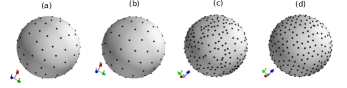
Figure 5: Sampling distribution from an optimized sensing matrix from spherical harmonics. (a) ALM $\left(K=97,N=9\right)$ (b) Grad. Descent $\left(K=97,N=9\right)$ (c) $\acs{ALM}\left(K=400,N=21\right)$ (d) Grad. Descent $\left(K=400,N=21\right)$

The phase transition diagram is depicted in Fig. 6. It can be seen that the optimized sensing matrix yields a performance similar to the random sampling’s, and shows a better recovery compared to the spiral and Hammersley samplings.

Figure 6: Phase transition diagram for sparse recovery of spherical harmonics.

5.2 Specific Case: Practical SNF Measurements

In most cases, we only evaluate the order $\mu=\pm 1$ with linearly polarized probes for polarization angles $\chi=0$ and $\chi=\frac{\pi}{2}$. This condition is not contrived and has practical relevance, as discussed in [2, 26]. In addition, we can provide experimental data from real measurements, which makes this case even more interesting, as explained in Section 3.2. Additionally, in this section we perform the far-field reconstruction with fewer sampling points, i.e., $K<L$, compared to the conventional settings that require a total of $K>2L$ measurements.

Figure 7: Coherence of sensing matrices for practical SNF measurements.

Since we only consider $\mu=\pm 1$ and polarization angles $\chi=0$ and $\chi=\frac{\pi}{2}$, we only optimize the elevation $\theta$ and azimuth $\phi$ angles. Fig. 7 presents the coherence of the sensing matrix from a specific setting constructed from several sampling points. The difference between this specific case compared to the general case in the previous section is that our sensing matrix results from concatenating the matrix constructed from Wigner D-functions for both values of $\chi$ considered, as derived in (8). The optimized sensing matrix, again, produces lower coherence compared to known deterministic sampling schemes.

Figure 8: Phase transition diagram for sparse recovery for practical SNF measurements.

Furthermore, the optimized sensing matrix also shows higher recovery chances than the spiral and Hammersley sampling schemes, as depicted in Fig. 8. Moreover, compared to random sampling points with arbitrary polarization angles $\chi$, the optimized sampling points deliver a similar performance while keeping the polarization angles alternate between $\chi=0$ and $\chi=\frac{\pi}{2}$.

6 Conclusions

We have discussed the methods to optimize sensing matrices for the CS-based SNF method. In contrast to the conventional method, which requires an oversampled near-field measurement, the CS-based method can significantly reduce the number of samples to reconstruct the far-field pattern by using an optimized sensing matrix. The strategy emanates from the fact that, in most cases, the SMCs are compressible. Harnessing this information is key in implementing the CS-based method.

We propose two different approaches, namely gradient-based and ALM based proximal methods, to design low coherence sensing matrices that are suitable for the CS-based method. Numerical experiments show that these approaches are successful in minimizing the coherence of sensing matrices constructed from Wigner D-functions and spherical harmonics. Numerical simulations from measurement data show that the proposed sampling schemes can reconstruct the far-field pattern with a reasonable error while reducing the number of sampling points. Additionally, numerical experiments show that the optimization methods maintain the uniformity structure of proposed sampling points, hence making it easier to implement in real measurement system.

Notation

The vectors and matrices are denoted by bold small-cap letters $\mathbf{a}$ and big-cap letters $\mathbf{A}$. The elevation, azimuth, and polarization angles are denoted by $\theta\in[0,\pi]$, $\phi\in[0,2\pi)$, and $\chi\in[0,2\pi)$, respectively. The set $\{1,...,m\}$ is denoted by $[m]$. $\overline{x}$ is the conjugate of $x$. For a vector $\mathbf{x}\in\mathbb{C}^{L}$, the $\ell_{p}$-norm is given by $\left\|\mathbf{x}\right\|_{p}=\left(\sum_{i=1}^{L}\left|x_{i}\right|^{p}\right)^{1/p}$ for $p\in[1,\infty)$ and $\left\|\mathbf{x}\right\|_{\infty}=\underset{i\in[L]}{\text{max}}\left|x_{i}\right|$ for $p=\infty$.

References

- [1] O. Breinbjerg, “Spherical near-field antenna measurements — the most accurate antenna measurement technique,” in 2016 IEEE International Symposium on Antennas and Propagation (APSURSI), 2016, pp. 1019–1020.
- [2] Jesper E Hansen, Spherical near-field antenna measurements, vol. 26, IET, 1988.
- [3] OM Bucci, C Gennarelli, F D’Agostino, and C Savarese, “A new and efficient nf-ff transformation with spherical spiral scanning,” in IEEE Antennas and Propagation Society International Symposium. 2001 Digest. Held in conjunction with: USNC/URSI National Radio Science Meeting (Cat. No. 01CH37229). IEEE, 2001, vol. 2, pp. 629–632.
- [4] Fernando Rodriguez Varela, Belen Galocha Iraguen, and Manuel Sierra-Castaner, “Under-sampled spherical near-field antenna measurements with error estimation,” IEEE Transactions on Antennas and Propagation, vol. 68, no. 8, pp. 6364–6371, 2020.
- [5] LJ Foged, F Saccardi, F Mioc, and PO Iversen, “Spherical near field offset measurements using downsampled acquisition and advanced nf/ff transformation algorithm,” in 2016 10th European Conference on Antennas and Propagation (EuCAP). IEEE, 2016, pp. 1–3.
- [6] Fernando Rodriguez Varela, Belen Galocha Iraguen, and Manuel Sierra-Castaner, “Application of nonuniform fft to spherical near-field antenna measurements,” IEEE Transactions on Antennas and Propagation, vol. 68, no. 11, pp. 7571–7579, 2020.
- [7] Rasmus Cornelius, Arya Adiprakasa Bangun, and Dirk Heberling, “Investigation of different matrix solver for spherical near-field to far-field transformation,” in 2015 9th European Conference on Antennas and Propagation (EuCAP). IEEE, 2015, pp. 1–4.
- [8] Rasmus Cornelius, Dirk Heberling, Niklas Koep, Arash Behboodi, and Rudolf Mathar, “Compressed sensing applied to spherical near-field to far-field transformation,” in 2016 10th European Conference on Antennas and Propagation (EuCAP). IEEE, 2016, pp. 1–4.
- [9] Cosme Culotta-López, Kui Wu, and Dirk Heberling, “Radiation center estimation from near-field data using a direct and an iterative approach,” in Antenna Measurement Techniques Association Symposium (AMTA). IEEE, 2017, pp. 303–308.
- [10] Cosme Culotta-López, Fast Near-Field Antenna Measurements by Application of Compressed Sensing, Dissertation, RWTH Aachen University, 2021.
- [11] Emmanuel J Candes and Terence Tao, “Decoding by linear programming,” IEEE Transactions on Information Theory, vol. 51, no. 12, pp. 4203–4215, 2005.
- [12] Emmanuel J Candès, Justin Romberg, and Terence Tao, “Robust uncertainty principles: Exact signal reconstruction from highly incomplete frequency information,” IEEE Transactions on Information Theory, vol. 52, no. 2, pp. 489–509, 2006.
- [13] Afonso S Bandeira, Edgar Dobriban, Dustin G Mixon, and William F Sawin, “Certifying the restricted isometry property is hard,” IEEE transactions on information theory, vol. 59, no. 6, pp. 3448–3450, 2013.
- [14] Andreas M Tillmann and Marc E Pfetsch, “The computational complexity of the restricted isometry property, the nullspace property, and related concepts in compressed sensing,” Information Theory, IEEE Transactions on, vol. 60, no. 2, pp. 1248–1259, 2014.
- [15] Richard Obermeier and Jose Angel Martinez-Lorenzo, “Sensing matrix design via mutual coherence minimization for electromagnetic compressive imaging applications,” IEEE Transactions on Computational Imaging, vol. 3, no. 2, pp. 217–229, 2017.
- [16] Yao Yu, Athina P Petropulu, and H Vincent Poor, “Measurement matrix design for compressive sensing–based mimo radar,” IEEE Transactions on Signal Processing, vol. 59, no. 11, pp. 5338–5352, 2011.
- [17] Holger Rauhut and Rachel Ward, “Sparse recovery for spherical harmonic expansions,” Proceedings of 9th International Conference on Sampling Theory and Applications (SampTA 2011), Feb. 2011, arXiv: 1102.4097.
- [18] Nicolas Burq, Semyon Dyatlov, Rachel Ward, and Maciej Zworski, “Weighted Eigenfunction Estimates with Applications to Compressed Sensing,” SIAM Journal on Mathematical Analysis, vol. 44, no. 5, pp. 3481–3501, Jan. 2012.
- [19] Arya Bangun, Arash Behboodi, and Rudolf Mathar, “Sparse recovery in wigner-d basis expansion,” in 2016 IEEE Global Conference on Signal and Information Processing (GlobalSIP). IEEE, 2016, pp. 287–291.
- [20] Arya Bangun, Arash Behboodi, and Rudolf Mathar, “Sensing Matrix Design and Sparse Recovery on the Sphere and the Rotation Group,” IEEE Transactions on Signal Processing, pp. 1439–1454, 2020.
- [21] Bernd Hofmann, Ole Neitz, and Thomas F Eibert, “On the minimum number of samples for sparse recovery in spherical antenna near-field measurements,” IEEE Transactions on Antennas and Propagation, vol. 67, no. 12, pp. 7597–7610, 2019.
- [22] Arya Bangun, Arash Behboodi, and Rudolf Mathar, “Coherence Bounds for Sensing Matrices in Spherical Harmonics Expansion,” in 2018 IEEE International Conference on Acoustics, Speech and Signal Processing (ICASSP), Calgary, AB, Apr. 2018, pp. 4634–4638, IEEE.
- [23] Cosme Culotta-López, Arya Bangun, Arash Behboodi, Dirk Heberling, and Rudolf Mathar, “A compressed sampling for spherical near-field measurements,” in Antenna Measurement Techniques Association Symposium (AMTA). IEEE, 2018.
- [24] Rémi Gribonval and Morten Nielsen, “Sparse representations in unions of bases,” IEEE transactions on Information theory, vol. 49, no. 12, pp. 3320–3325, 2003.
- [25] L. Welch, “Lower Bounds on the Maximum Cross Correlation of Signals,” IEEE Transactions on Information Theory, vol. 20, no. 3, pp. 397–399, May 1974.
- [26] Paul F Wacker, “Non-planar near field measurements: Spherical scanning,” Final Report, 1975.
- [27] Arya Bangun, Arash Behboodi, and Rudolf Mathar, “Tight bounds on the mutual coherence of sensing matrices for wigner d-functions on regular grids,” Sampling Theory, Signal Processing and Data Analysis, vol. 19, 2021.
- [28] Neal Parikh and Stephen Boyd, “Proximal algorithms,” Foundations and Trends in optimization, vol. 1, no. 3, pp. 127–239, 2014.
- [29] John Duchi, Shai Shalev-Shwartz, Yoram Singer, and Tushar Chandra, “Efficient projections onto the l 1-ball for learning in high dimensions,” in Proceedings of the 25th international conference on Machine learning, 2008, pp. 272–279.
- [30] Arya Bangun, Signal Recovery on the Sphere from Compressive and Phaseless Measurements, Dissertation, RWTH Aachen University, 2020.
- [31] Edward B Saff and Amo BJ Kuijlaars, “Distributing many points on a sphere,” The mathematical intelligencer, vol. 19, no. 1, pp. 5–11, 1997.
- [32] Jianjun Cui and Willi Freeden, “Equidistribution on the sphere,” SIAM Journal on Scientific Computing, vol. 18, no. 2, pp. 595–609, 1997.
- [33] Junfeng Yang and Yin Zhang, “Alternating direction algorithms for -problems in compressive sensing,” SIAM journal on scientific computing, vol. 33, no. 1, pp. 250–278, 2011.