Factored Conditional Filtering: Tracking States and Estimating Parameters in High-Dimensional Spaces

Abstract

This paper introduces the factored conditional filter, a new filtering algorithm for simultaneously tracking states and estimating parameters in high-dimensional state spaces. The conditional nature of the algorithm is used to estimate parameters and the factored nature is used to decompose the state space into low-dimensional subspaces in such a way that filtering on these subspaces gives distributions whose product is a good approximation to the distribution on the entire state space. The conditions for successful application of the algorithm are that observations be available at the subspace level and that the transition model can be factored into local transition models that are approximately confined to the subspaces; these conditions are widely satisfied in computer science, engineering, and geophysical filtering applications. We give experimental results on tracking epidemics and estimating parameters in large contact networks that show the effectiveness of our approach.

Keywords: Bayesian filtering, particle filtering, parameter estimation, state space models, factorization.

1 Introduction

Consider an agent being employed to assist in controlling an epidemic. The environment for the agent is the territory where the epidemic is taking place, the people and their locations in the territory, transport services between locations in the territory, and so on. Observations available to the agent could include numbers of people with the disease, numbers of deaths and recoveries, test results, and so on. Actions for the agent could include advice to human experts about which tests to perform on which people, the location and duration of lockdowns, and so on.

The most fundamental capability needed of such an agent is to be able to track the state of an epidemic from observations. Assume that the territory of the epidemic is modelled by a graph, where nodes in the graph could represent any of people, households, neighbourhoods, suburbs, towns, or cities. There is an undirected edge between each pair of nodes for which transmission of the disease between the two nodes is possible. Thus the model employs a contact network. Such a model is more complex than the more typical compartmental model but provides more detail about the epidemic. A state consists of the contact network with nodes labelled by information about the epidemic at that node, for example, whether the person represented by that node is susceptible, exposed, infectious, or recovered. Suppose that the agent knows the transition model and observation model of the epidemic. Then it can track the epidemic by computing a state distribution at each time step. The agent uses knowledge of the state distribution to select actions. This paper is concerned only with the problem of tracking the state of contact networks, not selecting actions.

Considered more abstractly, for a fixed contact network, the state space can be modelled by a product space, where each element of the product space is a particular state of the epidemic. For given transition and observation models, the generic problem is that of filtering on a product space representing a graph. In addition, the graph may have tens or hundreds of thousands, or even millions, of nodes, so the problem is one of filtering in high dimensions. Furthermore, the transition and observation models may have parameters that need to be estimated by the filtering process. One contribution of this paper is a filtering algorithm for high-dimensional state spaces that estimates parameters as it tracks the states.

In high-dimensional spaces, exact inference is usually infeasible; in such cases it is necessary to resort to approximation. The two main kinds of approximation commonly employed are based on Monte Carlo methods and variational methods. For filtering, the Monte Carlo method is manifested in the form of particle filtering and we discuss this first.

A well-known fundamental difficulty with particle filtering in high dimensions is that two distinct probability measures in high-dimensional spaces are nearly mutually singular. (For example, in high dimensions, Gaussian distributions with the identity matrix as covariance matrix have nearly all their probability mass in a thin annulus around a hypersphere with radius $\sqrt{d}$, where $d$ is the dimension of the space. See the Gaussian Annulus Theorem of Blum et al. (2020). It follows that two distinct Gaussian distributions in a high-dimensional space are nearly mutually singular.) In particular, in high dimensions, the distribution obtained after a transition update and the distribution obtained after the subsequent observation update are nearly mutually singular. As a consequence, the particle family obtained by resampling gives a poor approximation of the distribution obtained from the observation update. Typically, what happens is that one particle from the transition update has (normalized) weight very nearly equal to one and so the resampled particle family degenerates to a single particle. See the discussion about this by Snyder et al. (2008), for example. Intuitively, the problem could be solved with a large enough particle family. Unfortunately, it has been shown that to avoid degeneracy the size of the particle family has to be at least exponential in the problem size. More precisely, the size of the particle family must be exponential in the variance of the observation log likelihood, which depends not only on the state dimension but also on the distribution after the state transition and the number and character of observations. Simulations confirm this result. For the details, see the work by Bengtsson et al. (2008); Bickel et al. (2008), and Snyder et al. (2008).

In spite of these difficulties, it is often possible to exploit structure in the form of spatial locality of a particular high-dimensional problem to filter effectively, and this will be the case for filtering epidemics. Let the state space be $\prod_{i=1}^{m}Y_{i}$ and $\{C_{1},\ldots,C_{p}\}$ a partition of the index set $\{1,\ldots,m\}$. Suppose, for $l=1,\ldots,p$, the size of $C_{l}$ is small and that observations are available for subspaces of the form $\prod_{i\in C_{l}}Y_{i}$. It may even be the case that each $C_{l}$ is a singleton. Then, since each $C_{l}$ is small, the degeneracy difficulties mentioned above do not occur for the observation update for each $\prod_{i\in C_{l}}Y_{i}$. In addition, an assumption needs to be made about the transition model. It is too much to expect there to be local transition models completely confined to each $\prod_{i\in C_{l}}Y_{i}$. If this were true, it would be possible to filter the entire space by independently filtering on each of the subspaces. But what is often true is that the domain of transition model for $\prod_{i\in C_{l}}Y_{i}$ depends only on a subset of the $Y_{j}$, where index $j$ is a neighbour of, or at least close by, an index in $C_{l}$. The use of such local transition models introduces an approximation of the state distribution but, as our experiments here indicate, the error can be surprisingly small even for epidemics on large graphs. The resulting algorithm is called the factored filter, and the particle version of it is similar to the local particle filter of Rebeschini (2014), and Rebeschini and Van Handel (2015). Note that we have adopted the name factored filter that is used in the artificial intelligence literature rather than local filter that is used in the data assimilation literature.

Next we discuss the use of variational methods in filtering. The general setting for this discussion is that of assumed density filtering for which the state distribution is approximated by a density from some suitable space of densities, often an exponential subfamily. Essentially, there is an approximation step at the end of the filtering algorithm in which the density obtained from the observation update is projected into the space of approximating densities. (See the discussion and references in Section 18.5.3 of Murphy (2012).) Here we concentrate on variational methods for this approximation. This is based on minimizing a divergence measure between two distributions. In variational inference Jordan et al. (1999); Blei et al. (2017), the corresponding optimization problem is to find $\operatorname*{argmin}_{q}\it{KL}(q\|p)$, where $q$ is the approximation of $p$; in expectation propagation Minka (2001b); Vehtari et al. (2020), the corresponding optimization problem is to find $\operatorname*{argmin}_{q}\it{KL}(p\|q)$. To present the variational algorithms at a suitable level of abstraction, the $\alpha$-divergence Minka (2005); Bishop (2006) is employed. This is defined by

$$D_{\alpha}(p\|q)=\frac{4}{1-\alpha^{2}}\left(1-\int_{Y}p^{(1+\alpha)/2}q^{(1-\alpha)/2}\;d\upsilon_{Y}\right),$$

where $\alpha\in\mathbb{R}$. Note that

$$\lim_{\alpha\rightarrow 1}D_{\alpha}(p\|q)=\it{KL}(p\|q)$$

$$\lim_{\alpha\rightarrow-1}D_{\alpha}(p\|q)=\it{KL}(q\|p),$$

so that, with a suitable choice of $\alpha$, forward (inclusive) KL-divergence or reverse (exclusive) KL-divergence or a combination of these can be specified. For each application, a value for $\alpha$ and a corresponding optimization algorithm are chosen for use in the variational algorithms.

Variational methods are an attractive alternative to Monte Carlo methods: often variational methods are faster than Monte Carlo methods and scale better. We note a further advantage of variational methods: they produce closed-form versions of state distributions in contrast to the Dirac mixture distributions produced by Monte Carlo methods. This means that the output of a variational method can be comprehensible to people. In the context of the general setting for filtering in Section 2 for which the aim is to acquire empirical beliefs, comprehensibility can be crucial for interrogating an agent to understand why it acted the way it did, to check for various kinds of bias, and so on.

Turning now to the problem of estimating parameters, for this we employ a conditional filter; the particle version of this filter is functionally similar, but structured in a different way, to the nested particle filter of Crisan and Miguez (2017, 2018). What is needed is a pair of mutually recursive filters: one is a particle filter for parameters and the other a filter for states that is conditional on the values of the parameter. The filter for parameters calls the conditional filter for states because it needs to use the current state distribution to approximate the observation likelihood for a particular value of the parameter. The conditional filter for states calls the filter for parameters because it needs to use the parameter particle family approximating the current parameter distribution.

Finally, putting the conditional filter and the factored filter together, we obtain the factored conditional filter that can both track states and estimate parameters in high-dimensional spaces. The parameter part of this algorithm is the same as for the non-factored case. However, the state part of this algorithm is different to the conditional filter because it is now factored.

In summary, the starting point for our development is the standard filter; the particle version of the standard filter is the bootstrap particle filter of Gordon et al. (1993). With such a filter, it is possible to track states in low-dimensional state spaces. One extension of the standard filter is the conditional filter; with such a filter, it is possible to track states and estimate parameters in low-dimensional state spaces. A different extension of the standard filter is the factored filter; with such a filter, it is possible to track states in high-dimensional state spaces. The factored conditional filter, which combines the notions of a conditional filter and a factored filter, makes it possible under certain circumstances to track states and estimate parameters in high-dimensional state spaces. For each of these four cases, there are basic, particle, and variational versions of the corresponding filter.

The main contributions of this paper are the following:

• We provide a framework for investigating the space of filtering algorithms at a suitable level of abstraction and we place factored conditional filtering in this framework.

• We propose basic, particle, and variational versions of algorithms for factored conditional filtering, which make it possible for suitable applications to simultaneously track states and estimate parameters in high-dimensional state spaces.

• We empirically evaluate the factored conditional filtering algorithms in the application domain of epidemics spreading on contact networks. For a variety of large real-world contact networks, we demonstrate that the algorithms are able to accurately track epidemic states and estimate parameters.

The paper is organised as follows. The paper begins with a general setting for an agent situated in some environment, where the agent can apply actions to the environment and can receive observations from the environment. The fundamental problem is to provide the agent with a method for acquiring from observations empirical beliefs which the agent can use to select actions to achieve its goals. For the purpose of acquisition, stochastic filtering, in a sense more general than is usually considered, is highly suitable. In the context of this setting, Section 2 outlines the general form of the transition and observation models, the standard, conditional, factored, and factored conditional filters, together with their basic, particle, and variational versions, and other relevant details. Section 3 introduces the application of primary interest in this paper: epidemics on contact networks. It describes the network model of epidemics and compares it with the more commonly used compartmental model. In Section 4, experimental results from the use of factored filters to track states of epidemic processes on contact networks are presented. In Section 5, experimental results from the employment of the factored conditional filters to track states and estimate parameters of epidemic processes on contact networks are reported. Section 6 covers related work. The conclusion is given in Section 7, which also suggests directions for future research. An appendix provides additional experimental results.

2 A General Setting for Filtering

This section introduces the theory of filtering on which the filtering algorithms in this paper depend. The account is informal, without precise definitions or statements of theorems; an extensive and rigorous account of the theory underlying the algorithms, and the statements and proofs of the results alluded to in this paper, are given by Lloyd (2022). The notation used in the paper will also be introduced here; it is deliberately as precise as possible to enable rigorous definitions, and statements and proofs of results given by Lloyd (2022).

First, here are some general notational conventions. Functions usually have their signature given explicitly: the notation $f:X\rightarrow Y$ means that $f$ is a function with domain $X$ and codomain $Y$. The notation $f:X\rightarrow Y\rightarrow Z$ means $f:X\rightarrow(Y\rightarrow Z)$, so that the codomain of $f$ is the function space $Z^{Y}$, consisting of all functions from $Y$ to $Z$. Denoting by $\mathcal{D}(Y)$ the set of densities on $Y$, a function $f:X\rightarrow\mathcal{D}(Y)$ can also be written as $f:X\rightarrow Y\rightarrow\mathbb{R}$. The notation $\triangleq$ means ‘stand(s) for’.

The lambda calculus is a convenient way of compactly and precisely defining anonymous functions. Let $X$ and $Y$ be sets, $x$ a variable ranging over values in $X$, and $\varphi$ an expression taking values in $Y$. Then $\lambda x.\varphi$ denotes the function from $X$ to $Y$ defined by $x\mapsto\varphi$, for all $x\in X$. The understanding is that, for each element $e$ of $X$, the corresponding value of the function is obtained by replacing each free occurrence of $x$ in $\varphi$ by $e$. For example, $\lambda x.x^{2}:\mathbb{R}\rightarrow\mathbb{R}$ denotes the square function defined by $x\mapsto x^{2}$, for all $x\in\mathbb{R}$. For another example, if $f:X\rightarrow Y\rightarrow Z$, then, for all $y\in Y$, $\lambda x.f(x)(y):X\rightarrow Z$ is the function defined by $x\mapsto f(x)(y)$, for all $x\in X$.

The notation $\int_{X}f\;d\upsilon$ denotes the (Lebesgue) integral of the real-valued, measurable function $f:X\rightarrow\mathbb{R}$, where $X$ is a measure space with measure $\upsilon$. If $X$ is a Euclidean space, then $\upsilon$ is often Lebesgue measure. If $X$ is a countable space and $\upsilon$ is counting measure on $X$, then $\int_{X}f\;d\upsilon=\sum_{x\in X}f(x)$.

2.1 The Setting

The setting for stochastic filtering is that of an agent situated in some environment, where the agent applies actions to the environment and receives observations from the environment. Let $A$ be the set of actions and $O$ the set of observations. For all $n\in\mathbb{N}_{0}$,

$$H_{n}\triangleq A\times O\times\cdots\times A\times O,$$

where there are $n$ occurrences of $A$ and $n$ occurrences of $O$. ($\mathbb{N}_{0}$ is the set of non-negative integers and $\mathbb{N}$ the set of positive integers.) $H_{n}$ is the set of all histories up to time $n$.

Suppose that there is a set $Y$ of states that the environment can be in and the agent needs an estimate of this state at each time step in order to choose actions to achieve its goals. The key concept needed for that is a so-called schema having the form

$$(\mu_{n}:H_{n}\rightarrow\mathcal{P}(Y))_{n\in\mathbb{N}_{0}}.$$

Thus a schema is a sequence of functions each having the set of histories $H_{n}$ at time $n$ as their domain and the set of probability measures on the space $Y$ as their codomain. For the development of the theory of filtering, $\mathcal{P}(Y)$ is the natural codomain; for a practical application, it may be more convenient to work with $\mathcal{D}(Y)$, the set of densities on the space $Y$. The density version of a schema has the form

$$(\breve{\mu}_{n}:H_{n}\rightarrow\mathcal{D}(Y))_{n\in\mathbb{N}_{0}},$$

where $\breve{\mu}_{n}$ indicates the density form of $\mu_{n}$. Informally, it is possible to regard either $\mathcal{P}(Y)$ or $\mathcal{D}(Y)$ as distributions on $Y$.

For each $h_{n}\in H_{n}$, there is a so-called empirical belief $\mu_{n}(h_{n}):\mathcal{P}(Y)$. Such a belief is called empirical because it is learned from observations. At time $n$, if $h_{n}$ is the history that has occurred, then $\mu_{n}(h_{n})$ is a distribution on the space $Y$. If $Y$ is the state space, this distribution is the state distribution given the history $h_{n}$ according to the underlying stochastic process; thus $\mu_{n}(h_{n})$ can be thought of as the ‘ground truth’ state distribution. An agent’s estimate, denoted by $\savestack{\tmpbox}{\stretchto{\scaleto{\scalerel*[width("\mu_{n}(h_{n})")]{\kern-0.6pt\bigwedge\kern-0.6pt}{\rule[-614.295pt]{4.30554pt}{614.295pt}}}{}}{0.5ex}}\stackon[1pt]{\mu_{n}(h_{n})}{\tmpbox}$, of the state distribution $\mu_{n}(h_{n})$ is used by the agent to select actions. In this paper, it is proposed that $\savestack{\tmpbox}{\stretchto{\scaleto{\scalerel*[width("\mu_{n}(h_{n})")]{\kern-0.6pt\bigwedge\kern-0.6pt}{\rule[-614.295pt]{4.30554pt}{614.295pt}}}{}}{0.5ex}}\stackon[1pt]{\mu_{n}(h_{n})}{\tmpbox}$ be computed by the agent using stochastic filtering. In only very few cases can $\mu_{n}(h_{n})$ be computed exactly by a filter; generally, for tractability reasons, the filter will need to make approximations.

Actually, the space $Y$ can be any space of interest to the agent, not just the state space. And then there is a schema, and empirical beliefs depending on the history, associated with the space $Y$. Thus, in general, an agent may have many empirical beliefs associated with various spaces $Y$, not just the state space. (More precisely, each empirical belief is associated with a stochastic process on $Y$, not just $Y$.) However, to understand the following discussion, it is sufficient to keep the state space case in mind.

Note that the definition of each $\mu_{n}:H_{n}\rightarrow\mathcal{P}(Y)$ is strongly constrained by the requirement that $\mu_{n}$ must be a regular conditional distribution. Intuitively this means that $\mu_{n}$ represents a conditional probabilistic relationship between the stochastic processes that generate actions in $A$, observations in $O$, and elements in $Y$; this regular conditional distribution assumption turns out to be crucial in the theory of filtering.

After each action is performed and each observation is received, the definition of $\mu_{n}(h_{n})$ needs to be updated to a modified definition for $\mu_{n+1}(h_{n+1})$ at the next time step by the filtering process. Stochastic filtering is the process of tracking the empirical belief $\mu_{n}(h_{n})$ over time. For this process, a transition model and an observation model are needed.

A transition model has the form

$$(\tau_{n}:H_{n-1}\times A\times Y\rightarrow\mathcal{P}(Y))_{n\in\mathbb{N}},$$

where each $\tau_{n}$ satisfies a certain regular conditional distribution assumption. The density version of a transition model has the form

$$(\breve{\tau}_{n}:H_{n-1}\times A\times Y\rightarrow\mathcal{D}(Y))_{n\in\mathbb{N}}.$$

This signature for the transition model is unusual in that it includes $H_{n-1}$ in the domain. It turns out that it is natural for the general theory to include the history space in the domain; under a certain conditional independence assumption that holds for state spaces, the history argument can be dropped to recover the more usual definition of a transition model.

An observation model has the form

$$(\xi_{n}:H_{n-1}\times A\times Y\rightarrow\mathcal{P}(O))_{n\in\mathbb{N}},$$

where each $\xi_{n}$ satisfies a certain regular conditional distribution assumption. The density version of an observation model has the form

$$(\breve{\xi}_{n}:H_{n-1}\times A\times Y\rightarrow\mathcal{D}(O))_{n\in\mathbb{N}}.$$

Similarly, it turns out that it is natural for the general theory to include the history and action spaces in the domain of an observation model; under a certain conditional independence assumption that holds for state spaces, the history and action arguments can be dropped to recover the more usual definition of an observation model.

The regular conditional distribution assumptions ensure that schemas, transition models, and observation models are essentially unique with respect to the underlying stochastic processes.

The setting is sufficiently general to provide a theoretical framework for the acquisition of empirical beliefs by an agent situated in some environment. Furthermore, empirical beliefs can be far more general than the standard case of state distributions.

To better appreciate factored conditional filtering we introduce in this paper, it is useful to place it in the space of filtering algorithms. For this reason, in the next four subsections, we provide a framework for filters based on their main characteristics, such as being factored or conditional, as well as being Monte Carlo or variational. This leads to 12 filters in all. There are the four different groups of standard, conditional, factored, and factored conditional. Inside each group there are 3 algorithms depending on whether they are basic, particle or variational filters. These 12 algorithms are summarized in Table 1.

2.2 Standard Filtering

Suppose now that the empirical belief $\breve{\mu}_{n-1}(h_{n-1}):\mathcal{D}(Y)$ at time $n-1$ is known. Given the action $a_{n}$ applied by the agent and the observation $o_{n}$ received from the environment, the agent needs to compute the empirical belief $\breve{\mu}_{n}(h_{n}):\mathcal{D}(Y)$ at the next time step. This is achieved by first applying the transition model $\breve{\tau}_{n}$ to the empirical belief $\breve{\mu}_{n-1}(h_{n-1})$ in the transition update to obtain the intermediate distribution

$$\lambda y.\int_{Y}\lambda y^{\prime}.\breve{\tau}_{n}(h_{n-1},a_{n},y^{\prime})(y)\;\breve{\mu}_{n-1}(h_{n-1})\;d\upsilon_{Y}$$

on $Y$. (For a fixed $y$, $\lambda y^{\prime}.\breve{\tau}_{n}(h_{n-1},a_{n},y^{\prime})(y)$ is a real-valued function on $Y$. Also $\breve{\mu}_{n-1}(h_{n-1})$ is a real-valued function on $Y$. Multiply these two functions together and then integrate the product. Now let $y$ vary to get the new distribution on $Y$.) Here, $\upsilon_{Y}$ is the underlying measure on the space $Y$. Then, in the observation update, the observation model and the actual observation are used to modify the intermediate distribution to obtain $\breve{\mu}_{n}(h_{n})$ via

$$\breve{\mu}_{n}(h_{n})=K^{-1}\,\lambda y.\breve{\xi}_{n}(h_{n-1},a_{n},y)(o_{n})\;\lambda y.\int_{Y}\lambda y^{\prime}.\breve{\tau}_{n}(h_{n-1},a_{n},y^{\prime})(y)\;\breve{\mu}_{n-1}(h_{n-1})\;d\upsilon_{Y},$$

where $K$ is a normalization constant. There is also a probability measure version of the preceding filter recurrence equation. The corresponding algorithm for the standard filter is given in Algorithm 1. (This is the basic version of the standard filter.)

Algorithm 1 Standard Filter
returns Empirical belief $\breve{\mu}_{n}(h_{n})$ at time $n$
inputs: Empirical belief $\breve{\mu}_{n-1}(h_{n-1})$ at time $n-1$,
  history $h_{n-1}$ up to time $n-1$,
  action $a_{n}$ at time $n$,
  observation $o_{n}$ at time $n$.

1:  $\displaystyle{\breve{\overline{\mu}}_{n}(h_{n-1},a_{n}):=\lambda y.\int_{Y}\lambda y^{\prime}.\breve{\tau}_{n}(h_{n-1},a_{n},y^{\prime})(y)\;\breve{\mu}_{n-1}(h_{n-1})\;d\upsilon_{Y}}$

2:  $\displaystyle{\breve{\mu}_{n}(h_{n}):=\frac{\lambda y.\breve{\xi}_{n}(h_{n-1},a_{n},y)(o_{n})\;\breve{\overline{\mu}}_{n}(h_{n-1},a_{n})}{\int_{Y}\lambda y.\breve{\xi}_{n}(h_{n-1},a_{n},y)(o_{n})\;\breve{\overline{\mu}}_{n}(h_{n-1},a_{n})\;d\upsilon_{Y}}}$

3:  return  $\breve{\mu}_{n}(h_{n})$

Particle versions of the filter of Algorithm 1 are widely used in practice. In this case, empirical beliefs are approximated by mixtures of Dirac measures, so that

$$\mu_{n}(h_{n})\approx\frac{1}{N}\sum_{i=1}^{N}\delta_{y_{n}^{(i)}},$$

where each particle $y_{n}^{(i)}\in Y$ and each $\delta_{y_{n}^{(i)}}$ is the Dirac measure at $y_{n}^{(i)}$. Particle filters have the advantage of being applicable when closed-form expressions for the $\mu_{n}(h_{n})$ are not available from the filter recurrence equations, as is usually the case. The corresponding particle filter, which can be derived from Algorithm 1, is given in Algorithm 2 below.

Given the particle family $(y_{n-1}^{(i)})_{i=1}^{N}$ at time $n-1$, the history $h_{n-1}$, as well as the action $a_{n}$ and observation $o_{n}$ at time $n$, the standard particle filter as shown in Algorithm 2 produces the particle family $(y_{n}^{(i)})_{i=1}^{N}$ at time $n$ using the transition model $\tau$ (via the transition update in Line 2) and the observation model $\breve{\xi}$ (via the observation update in Line 3). The resampling step (Line 9) with respect to the normalized weights of particles (Line 6) serves to alleviate the degeneracy of particles Gordon et al. (1993).

Algorithm 2 Standard Particle Filter
returns Particle family $(y_{n}^{(i)})_{i=1}^{N}$ at time $n$
inputs: Particle family $(y_{n-1}^{(i)})_{i=1}^{N}$ at time $n-1$,
  history $h_{n-1}$ up to time $n-1$,
  action $a_{n}$ at time $n$,
  observation $o_{n}$ at time $n$.

1:  for $i:=1$ to $N$ do

2:     sample $\overline{y}_{n}^{(i)}\sim\frac{1}{N}\sum_{i^{\prime}=1}^{N}\tau_{n}(h_{n-1},a_{n},y_{n-1}^{(i^{\prime})})$

3:     $w_{n}^{(i)}:=\breve{\xi}_{n}(h_{n-1},a_{n},\overline{y}_{n}^{(i)})(o_{n})$

4:  end for

5:  for $i:=1$ to $N$ do

6:     $\overline{w}_{n}^{(i)}:=\frac{w_{n}^{(i)}}{\sum_{i^{\prime}=1}^{N}w_{n}^{(i^{\prime})}}$

7:  end for

8:  for $i:=1$ to $N$ do

9:     sample $y_{n}^{(i)}\sim\sum_{i^{\prime}=1}^{N}\overline{w}_{n}^{(i^{\prime})}\delta_{\overline{y}_{n}^{(i^{\prime})}}$

10:  end for

11:  return  $(y_{n}^{(i)})_{i=1}^{N}$

Algorithm 3 is a variational version of the standard filter. It is an assumed density filter for which the approximation step is based on a variational principle. Line 1 is the transition update using the approximation $q_{n-1}$ of $\breve{\mu}_{n-1}(h_{n-1})$. In Line 2, the density $p_{n}$ is obtained from the observation update. Line 3 is the variational update. For this, $Q\subseteq\mathcal{D}(Y)$ is a suitable subclass of densities on $Y$ from which the approximation to $\breve{\mu}_{n}(h_{n})$ is chosen; for example, $Q$ could be some subclass of the exponential family of distributions. The density $q_{n}\in Q$ that minimizes the $\alpha$–divergence $D_{\alpha}(p_{n}\|q)$ between $p_{n}$ and $q\in Q$ is computed. Depending on the application, a value for $\alpha$ and a corresponding optimization algorithm are chosen. Thus Algorithm 3 allows the particular method of variational approximation to depend upon the application. For example, a common choice for Algorithm 3 could be that of reverse KL-divergence as the divergence measure and variational inference as the approximation method.

Algorithm 3 Standard Variational Filter
returns Approximation $q_{n}$ of empirical belief $\breve{\mu}_{n}(h_{n})$ at time $n$
inputs: Approximation $q_{n-1}$ of empirical belief $\breve{\mu}_{n-1}(h_{n-1})$ at time $n-1$,
  history $h_{n-1}$ up to time $n-1$,
  action $a_{n}$ at time $n$,
  observation $o_{n}$ at time $n$.

1:  $\displaystyle{\overline{q}_{n}:=\lambda y.\int_{Y}\lambda y^{\prime}.\breve{\tau}_{n}(h_{n-1},a_{n},y^{\prime})(y)\;q_{n-1}\;d\upsilon_{Y}}$

2:  $\displaystyle{p_{n}:=\frac{\lambda y.\breve{\xi}_{n}(h_{n-1},a_{n},y)(o_{n})\;\overline{q}_{n}}{\int_{Y}\lambda y.\breve{\xi}_{n}(h_{n-1},a_{n},y)(o_{n})\;\overline{q}_{n}\;d\upsilon_{Y}}}$

3:  $\displaystyle{q_{n}:=\operatorname*{argmin}_{q\in Q}D_{\alpha}(p_{n}\|q)}$

4:  return  $q_{n}$

2.3 Conditional Filtering

It is common when filtering to also need to estimate some unknown parameters in the transition and observation models. This can be handled elegantly with conditional filters, in a way that, at least for a conditional particle filter, is similar to the nested particle filter of Crisan and Miguez (2017, 2018). Suppose the parameter space is $X$. Then $X$ becomes an argument of the domains for the schema, transition model, and observation model. Thus, in the conditional case, a schema has the form

$$(\mu_{n}:H_{n}\times X\rightarrow\mathcal{P}(Y))_{n\in\mathbb{N}_{0}},$$

a transition model has the form

$$(\tau_{n}:H_{n-1}\times A\times X\times Y\rightarrow\mathcal{P}(Y))_{n\in\mathbb{N}},$$

and an observation model has the form

$$(\xi_{n}:H_{n-1}\times A\times X\times Y\rightarrow\mathcal{P}(O))_{n\in\mathbb{N}}.$$

In this setting, empirical beliefs from $X$ to $Y$ have the form $\lambda x.\mu_{n}(h_{n},x):X\rightarrow\mathcal{P}(Y)$, where $h_{n}\in H_{n}$.

In addition, there is a schema, transition model, and observation model for the parameter space $X$:

$$(\nu_{n}:H_{n}\rightarrow\mathcal{P}(X))_{n\in\mathbb{N}_{0}},$$

$$(\eta_{n}:H_{n-1}\times A\times X\rightarrow\mathcal{P}(X))_{n\in\mathbb{N}},\text{ and}$$

$$(\zeta_{n}:H_{n-1}\times A\times X\rightarrow\mathcal{P}(O))_{n\in\mathbb{N}}.$$

The conditional filter is given in Algorithm 4. (This is the basic version of the conditional filter.) A filter is set up on $X$ and a conditional filter is set up on $Y$ that is conditional on $X$. The filter on $X$ is just the (standard) filter in Algorithm 1 or its particle version in Algorithm 2, with schema $\nu$, transition model $\eta$, and observation model $\zeta$. On $Y$, the conditional filter is just the conditionalized version of the standard filter. An assumption sufficient to prove the correctness of Algorithm 4 is that the actual value of the parameter in $X$ be fixed; this condition is satisfied for the applications considered in this paper.

Algorithm 4 Conditional Filter
returns Empirical belief $\lambda x.\breve{\mu}_{n}(h_{n},x)$ at time $n$
inputs: Empirical belief $\lambda x.\breve{\mu}_{n-1}(h_{n-1},x)$ at time $n-1$,
  history $h_{n-1}$ up to time $n-1$,
  action $a_{n}$ at time $n$,
  observation $o_{n}$ at time $n$.

1:  $\displaystyle{\lambda x.\breve{\overline{\mu}}_{n}(h_{n-1},a_{n},x):=\lambda x.\lambda y.\int_{Y}\lambda y^{\prime}.\breve{\tau}_{n}(h_{n-1},a_{n},x,y^{\prime})(y)\;\breve{\mu}_{n-1}(h_{n-1},x)\;d\upsilon_{Y}}$

2:  $\displaystyle{\lambda x.\breve{\mu}_{n}(h_{n},x):=\lambda x.\frac{\lambda y.\breve{\xi}_{n}(h_{n-1},a_{n},x,y)(o_{n})\;\breve{\overline{\mu}}_{n}(h_{n-1},a_{n},x)}{\int_{Y}\lambda y.\breve{\xi}_{n}(h_{n-1},a_{n},x,y)(o_{n})\;\breve{\overline{\mu}}_{n}(h_{n-1},a_{n},x)\;d\upsilon_{Y}}}$

3:  return  $\lambda x.\breve{\mu}_{n}(h_{n},x)$

There is a particle version of Algorithm 4. For conditional particle filters, particle families also have to be conditionalized. A conditional particle (from $X$ to $Y$) is a pair $(x,(y^{(j)})_{j=1}^{M})$, where $x$ is a particle in $X$ and $(y^{(j)})_{j=1}^{M}$ is a particle family in $Y$. A conditional particle family (from $X$ to $Y$) is an indexed family of the form $((x^{(i)},(y^{(i,j)})_{j=1}^{M}))_{i=1}^{N}$, where each $(x^{(i)},(y^{(i,j)})_{j=1}^{M})$ is a conditional particle. So a conditional particle family is an indexed family of conditional particles. The empirical beliefs $\nu_{n}(h_{n}):\mathcal{P}(X)$ and $\lambda x.\mu_{n}(h_{n},x):X\rightarrow\mathcal{P}(Y)$ together are approximated by a conditional particle family $((x^{(i)}_{n},(y^{(i,j)}_{n})_{j=1}^{M}))_{i=1}^{N}$. More precisely,

$$\nu_{n}(h_{n})\approx\frac{1}{N}\sum_{i=1}^{N}\delta_{x^{(i)}_{n}},\text{ and}$$

$$\mu_{n}(h_{n},x^{(i)}_{n})\approx\frac{1}{M}\sum_{j=1}^{M}\delta_{y^{(i,j)}_{n}},\text{ for }i=1,\ldots,N.$$

The conditional particle filter is given in Algorithm 5 below. This algorithm parallels the standard particle filter (Algorithm 2); Line 3 is the transition update, Line 4 the observation update, and Line 10 the resampling step.

Algorithm 5 Conditional Particle Filter
returns Conditional particle family $((x_{n}^{(i)},(y_{n}^{(i,j)})_{j=1}^{M}))_{i=1}^{N}$ at time $n$
inputs: Particle family $(x_{n}^{(i)})_{i=1}^{N}$ at time $n$,
  conditional particle family $((x_{n-1}^{(i)},(y_{n-1}^{(i,j)})_{j=1}^{M}))_{i=1}^{N}$ at time $n-1$,
  history $h_{n-1}$ up to time $n-1$,
  action $a_{n}$ at time $n$,
  observation $o_{n}$ at time $n$.

1:  for $i:=1$ to $N$ do

2:     for $j:=1$ to $M$ do

3:        sample $\overline{y}_{n}^{(i,j)}\sim\frac{1}{M}\sum_{j^{\prime}=1}^{M}\tau_{n}(h_{n-1},\,a_{n},\,x_{n}^{(i)},\,y_{n-1}^{(i^{*},j^{\prime})})$

4:        $w_{n}^{(i,j)}:=\breve{\xi}_{n}(h_{n-1},\,a_{n},\,x_{n}^{(i)},\,\overline{y}_{n}^{(i,j)})(o_{n})$

5:     end for

6:     for $j:=1$ to $M$ do

7:        $\overline{w}_{n}^{(i,j)}:=\frac{w_{n}^{(i,j)}}{\sum_{j^{\prime}=1}^{M}w_{n}^{(i,j^{\prime})}}$

8:     end for

9:     for $j:=1$ to $M$ do

10:        sample $y_{n}^{(i,j)}\sim\sum_{j^{\prime}=1}^{M}\overline{w}_{n}^{(i,j^{\prime})}\delta_{\overline{y}_{n}^{(i,j^{\prime})}}$

11:     end for

12:  end for

13:  return  $((x_{n}^{(i)},(y_{n}^{(i,j)})_{j=1}^{M}))_{i=1}^{N}$

Some explanation of the index $i^{*}$ in Line 3 of Algorithm 5 is necessary. Recall that, for the correctness of the conditional filter, the unknown parameter is assumed to be fixed. This implies that the transition model $\eta$ in the filter for the parameter (Algorithm 2, for the space $X$) should be a no-op having the definition $\eta_{n}=\lambda(h,a,x).\delta_{x}$, for all $n\in\mathbb{N}$. In this case, the transition update in Line 2 of Algorithm 2 is

$$\text{sample }\overline{x}^{(i)}_{n}\sim\frac{1}{N}\sum_{i^{\prime}=1}^{N}\delta_{x^{(i^{\prime})}_{n-1}}.$$

If Algorithm 5 is used in combination with this version of Algorithm 2, then $x^{(i)}_{n}=x^{(i^{*})}_{n-1}$, for some $i^{*}\in\{1,\ldots,N\}$. This value of $i^{*}$ is used in Line 3 of Algorithm 5.

However, in practice, this property of the transition model being a no-op can lead to degeneracy of the parameter particle family. Thus a jittering transition model is used instead Crisan and Miguez (2018). Instead of keeping the parameter fixed, the transition model perturbs it slightly, thus avoiding degeneracy, as shown by Chopin et al. (2013), and Crisan and Miguez (2018). Commonly, the parameter space $X$ is $\mathbb{R}^{m}$, for some $m\geq 1$. For this case, $\breve{\eta}_{n}$ is defined, for all $n\in\mathbb{N}$, by

$$\breve{\eta}_{n}=\lambda(h,a,x).\mathcal{N}(x,\Sigma_{n}),$$

where $\mathcal{N}(\mu,\Sigma)$ denotes the Gaussian density with mean $\mu$ and covariance matrix $\Sigma$, and $\Sigma_{n}$ is a (diagonal) covariance matrix with suitably small diagonal values that may change over time according to some criterion in case the jittering is adaptive. With this modification, Line 2 of Algorithm 2 now becomes

$$\text{sample }\overline{x}_{n}^{(i)}\sim\frac{1}{N}\sum_{i^{\prime}=1}^{N}\mathcal{N}(x_{n-1}^{(i^{\prime})},\,\Sigma_{n}).$$

If Algorithm 5 is used in combination with this version of Algorithm 2, then $x^{(i)}_{n}\sim\mathcal{N}(x^{(i^{*})}_{n-1},\Sigma_{n})$, for some $i^{*}\in\{1,\ldots,N\}$. Thus $x^{(i)}_{n}$ is a perturbation of $x^{(i^{*})}_{n-1}$. This is the version of Algorithm 2 that is used in the paper for estimating parameters in the applications.

There is a crucial result concerning the observation update in Line 3 of Algorithm 2 (for the space $X$),

$$w_{n}^{(i)}:=\breve{\zeta}_{n}(h_{n-1},a_{n},\overline{x}_{n}^{(i)})(o_{n}),$$

that makes it possible to estimate parameters using a conditional filter. The transition model $\tau$, the observation model $\xi$, and the transition model $\eta$ can be expected to be known by the designer of the system (except perhaps for some parameters in $\tau$ and $\xi$). But the observation model $\zeta$ is generally not obvious at all. Fortunately, $\zeta$ can be computed at each time step from other information that is known. There is a result, called observation model synthesis, which states that, for all $n\in\mathbb{N}_{0}$ and (almost) all $h_{n}\in H_{n}$, $a_{n+1}\in A$, $x\in X$, and $o\in O$,

$$\breve{\zeta}_{n+1}(h_{n},a_{n+1},x)(o)=\int_{Y}\lambda y.\breve{\xi}_{n+1}(h_{n},a_{n+1},x,y)(o)\;d(\mu_{n}(h_{n},x)\odot\lambda y.\tau_{n+1}(h_{n},a_{n+1},x,y)).$$

(If $\mu_{1}:\mathcal{P}(X_{1})$ and $\mu_{2}:X_{1}\rightarrow\mathcal{P}(X_{2})$, then $\mu_{1}\odot\mu_{2}:\mathcal{P}(X_{2})$ is defined by $\mu_{1}\odot\mu_{2}=\lambda A_{2}.\int_{X_{1}}\lambda x_{1}.\mu_{2}(x_{1})(A_{2})\;d\mu_{1}$.) Thus $\breve{\zeta}_{n+1}$ can be constructed from the known $\breve{\xi}_{n+1}$, $\mu_{n}$, and $\tau_{n+1}$. It follows that the observation update in Line 3 of Algorithm 2 (for the space $X$) can be replaced by

$$w_{n}^{(i)}:=\int_{Y}\lambda y.\breve{\xi}_{n}(h_{n-1},a_{n},\overline{x}_{n}^{(i)},y)(o_{n}){\;d}(\mu_{n-1}(h_{n-1},\overline{x}_{n}^{(i)})\odot\lambda y.\tau_{n}(h_{n-1},a_{n},\overline{x}_{n}^{(i)},y)).$$

where the integral can be approximated using Monte Carlo integration by sampling from the probability measure $\mu_{n-1}(h_{n-1},\overline{x}_{n}^{(i)})\odot\lambda y.\tau_{n}(h_{n-1},a_{n},\overline{x}_{n}^{(i)},y)$. This is enough to allow the particle filter on $X$ to estimate the parameters accurately provided the approximation of the empirical belief from $X$ to $Y$ is accurate enough.

Hence, using the observation model synthesis result, we obtain the key Algorithm 2^∗ that is a specialization of Algorithm 2 for estimating parameters (where parameter distributions are approximated by particle families).

Algorithm 2 ^∗ Parameter Particle Filter
returns Particle family $(x_{n}^{(i)})_{i=1}^{N}$ at time $n$
inputs: particle family $(x_{n-1}^{(i)})_{i=1}^{N}$ at time $n-1$,
  empirical belief $\lambda x.\mu_{n-1}(h_{n-1},x)$ at time $n-1$,
  history $h_{n-1}$ up to time $n-1$,
  action $a_{n}$ at time $n$,
  observation $o_{n}$ at time $n$.

1:  for $i:=1$ to $N$ do

2:     sample $\overline{x}^{(i)}_{n}\sim\frac{1}{N}\sum_{i^{\prime}=1}^{N}\mathcal{N}(x^{(i^{\prime})}_{n-1},\Sigma_{n})$

3:     $w_{n}^{(i)}:=\int_{Y}\lambda y.\breve{\xi}_{n}(h_{n-1},a_{n},\overline{x}_{n}^{(i)},y)(o_{n}){\;d}(\mu_{n-1}(h_{n-1},\overline{x}_{n}^{(i)})\odot\lambda y.\tau_{n}(h_{n-1},a_{n},\overline{x}_{n}^{(i)},y))$

4:  end for

5:  for $i:=1$ to $N$ do

6:     $\overline{w}_{n}^{(i)}:=\frac{w_{n}^{(i)}}{\sum_{i^{\prime}=1}^{N}w_{n}^{(i^{\prime})}}$

7:  end for

8:  for $i:=1$ to $N$ do

9:     sample $x_{n}^{(i)}\sim\sum_{i^{\prime}=1}^{N}\overline{w}_{n}^{(i^{\prime})}\delta_{\overline{x}_{n}^{(i^{\prime})}}$

10:  end for

11:  return  $(x_{n}^{(i)})_{i=1}^{N}$

In fact, there is a further specialization of Algorithm 2^∗ for the case that state distributions are also approximated by particle families. Towards this, note that the immediately preceding statement in Line 2 of Algorithm 2,

$$\text{sample }\overline{x}^{(i)}_{n}\sim\frac{1}{N}\sum_{i^{\prime}=1}^{N}\mathcal{N}(x^{(i^{\prime})}_{n-1},\Sigma_{n}),$$

shows that $\overline{x}^{(i)}_{n}\sim\mathcal{N}(x^{(i^{*})}_{n-1},\Sigma_{n})$, for some $i^{*}\in\{1,\ldots,N\}$. Thus the observation update in Line 3 of Algorithm 2 (for the space $X$) can be approximated by

$$w_{n}^{(i)}:=\int_{Y}\lambda y.\breve{\xi}_{n}(h_{n-1},a_{n},\overline{x}_{n}^{(i)},y)(o_{n}){\;d}\frac{1}{M}\sum_{j=1}^{M}\tau_{n}(h_{n-1},a_{n},\overline{x}_{n}^{(i)},y_{n-1}^{(i^{*},j)}),$$ (1)

where the integral can be approximated using Monte Carlo integration by sampling from the probability measure $\frac{1}{M}\sum_{j=1}^{M}\tau_{n}(h_{n-1},a_{n},\overline{x}_{n}^{(i)},y_{n-1}^{(i^{*},j)})$.

Putting the above modifications together, we obtain Algorithm 2^∗∗, which is a variant of Algorithm 2 that is specialized for estimating parameters (where both parameter and state distributions are approximated by particle families). Both Algorithms 2^∗ and 2^∗∗ are used later in applications in this paper.

Algorithm 2 ^∗∗ Parameter Particle Filter
returns Particle family $(x_{n}^{(i)})_{i=1}^{N}$ at time $n$
inputs: Conditional particle family $((x_{n-1}^{(i)},(y_{n-1}^{(i,j)})_{j=1}^{M}))_{i=1}^{N}$ at time $n-1$,
  history $h_{n-1}$ up to time $n-1$,
  action $a_{n}$ at time $n$,
  observation $o_{n}$ at time $n$.

1:  for $i:=1$ to $N$ do

2:     sample $\overline{x}^{(i)}_{n}\sim\frac{1}{N}\sum_{i^{\prime}=1}^{N}\mathcal{N}(x^{(i^{\prime})}_{n-1},\Sigma_{n})$

3:     $w_{n}^{(i)}:=\int_{Y}\lambda y.\breve{\xi}_{n}(h_{n-1},a_{n},\overline{x}_{n}^{(i)},y)(o_{n}){\;d}\frac{1}{M}\sum_{j=1}^{M}\tau_{n}(h_{n-1},a_{n},\overline{x}_{n}^{(i)},y_{n-1}^{(i^{*},j)})$

4:  end for

5:  for $i:=1$ to $N$ do

6:     $\overline{w}_{n}^{(i)}:=\frac{w_{n}^{(i)}}{\sum_{i^{\prime}=1}^{N}w_{n}^{(i^{\prime})}}$

7:  end for

8:  for $i:=1$ to $N$ do

9:     sample $x_{n}^{(i)}\sim\sum_{i^{\prime}=1}^{N}\overline{w}_{n}^{(i^{\prime})}\delta_{\overline{x}_{n}^{(i^{\prime})}}$

10:  end for

11:  return  $(x_{n}^{(i)})_{i=1}^{N}$

The combination of Algorithms 2^∗∗ and 5 is similar to, but not identical with, the nested particle filter of Crisan and Miguez (2017, 2018). For the former, there is a filter for the parameters and also a conditional filter for the states; in contrast, for Crisan and Miguez (2017, 2018), there is a single filter for parameters and states together. As a consequence, operations in the nested particle filter are performed in a different order to the algorithm presented here. Furthermore, Crisan and Miguez (2017, 2018) handle resampling of parameters differently in that conditional particles that consist of both a parameter particle and a state particle family are resampled based on the weights of the parameters alone. Nevertheless, the outputs of the nested particle filter and the combination of Algorithms 2^∗∗ and 5 are very similar, as is evidenced by the experimental results given in the Appendix. The theoretical results for the nested particle filter of Crisan and Miguez (2017, 2018) also apply to the combination of Algorithms 2^∗∗ and 5 here; these include Theorems 2 and 3 of Crisan and Miguez (2018) on asymptotic convergence of the approximation errors in $L_{p}$ and Theorems 1 and 2 of Crisan and Miguez (2017) on uniform convergence in time.

To end this subsection, Algorithm 6 is the conditional variational filter. Let $Q\subseteq\mathcal{D}(Y)$ be a suitable class of densities; for example, $Q$ could be a subclass of the exponential family of distributions. The approximation to $\lambda x.\breve{\mu}_{n}(h_{n},x)$ is chosen from the space $Q^{X}$ of conditional densities. Line 3 returns the $q\in Q^{X}$ that minimizes the average of the conditional $\alpha$-divergence $\lambda x.D_{\alpha}(p_{n}(x)\|q(x))$ with respect to the empirical belief $\breve{\nu}_{n}(h_{n}):\mathcal{D}(X)$. The probability measure version of Line 3 is

$$q_{n}:=\operatorname*{argmin}_{q\in Q^{X}}\int_{X}\lambda x.D_{\alpha}(p_{n}(x)\|q(x))\;d\nu_{n}(h_{n}).$$

Algorithm 6 Conditional Variational Filter
returns Approximation $q_{n}$ of the empirical belief $\lambda x.\breve{\mu}_{n}(h_{n},x)$ at time $n$
inputs: Empirical belief $\breve{\nu}_{n}(h_{n})$ at time n,
  approximation $q_{n-1}$ of the empirical belief $\lambda x.\breve{\mu}_{n-1}(h_{n-1},x)$ at time $n-1$,
  history $h_{n-1}$ up to time $n-1$,
  action $a_{n}$ at time $n$,
  observation $o_{n}$ at time $n$.

1:  $\displaystyle{\overline{q}_{n}:=\lambda x.\lambda y.\int_{Y}\lambda y^{\prime}.\breve{\tau}_{n}(h_{n-1},a_{n},x,y^{\prime})(y)\;q_{n-1}(x)\;d\upsilon_{Y}}$

2:  $\displaystyle{p_{n}:=\lambda x.\frac{\lambda y.\breve{\xi}_{n}(h_{n-1},a_{n},x,y)(o_{n})\;\overline{q}_{n}(x)}{\int_{Y}\lambda y.\breve{\xi}_{n}(h_{n-1},a_{n},x,y)(o_{n})\;\overline{q}_{n}(x)\;d\upsilon_{Y}}}$

3:  $\displaystyle{q_{n}:=\operatorname*{argmin}_{q\in Q^{X}}\int_{X}\lambda x.D_{\alpha}(p_{n}(x)\|q(x))\,\breve{\nu}_{n}(h_{n})\;d\upsilon_{X}}$

4:  return  $q_{n}$

Commonly, the filter on the space $X$ is a standard particle filter. In this case, the variational update in Line 3 of Algorithm 6 is handled as follows. The empirical belief $\nu_{n}(h_{n})$ has the form $\frac{1}{N}\sum_{i=1}^{N}\delta_{x_{n}^{(i)}}$. Thus

$$\;\operatorname*{argmin}_{q\in Q^{X}}\int_{X}\lambda x.D_{\alpha}(p_{n}(x)\|q(x))\;d\nu_{n}(h_{n})$$

$$= \;\operatorname*{argmin}_{q\in Q^{X}}\frac{1}{N}\sum_{i=1}^{N}D_{\alpha}(p_{n}(x_{n}^{(i)})\|q(x_{n}^{(i)})).$$

Consequently, for $i=1,\ldots,N$,

$$q_{n}(x_{n}^{(i)})=\operatorname*{argmin}_{r\in Q}D_{\alpha}(p_{n}(x_{n}^{(i)})\|r).$$

Note that, if $x_{n}^{(i)}=x_{n}^{(j)}$, for $i\neq j$, then $q_{n}(x_{n}^{(i)})=q_{n}(x_{n}^{(j)})$. Also,

$$\nu_{n}(h_{n})(\{x\in X\;|\;x\neq x_{n}^{(i)},\text{ for }i=1,\ldots,N\})=0.$$

The values of $q_{n}$ outside the particle family $(x_{n}^{(i)})_{i=1}^{N}$ can be arbitrary. In summary, the variational update in Line 3 reduces to calculating $q_{n}(x_{n}^{(i)})$, for $i=1,\ldots,N$.

The filter on the space $X$ can also be a standard filter or a standard variational filter. In either case, for applications where $X$ is a structured space, one way to proceed is to restrict $q_{n}$ to range over the set of piecewise-constant conditional densities in $Q^{X}$. (A function $f:X\rightarrow Y$ is piecewise-constant if there exists a partition $(X_{i})_{i=1}^{n}$ of $X$ and a subset $\{y_{1},\ldots,y_{n}\}$ of $Y$ such that $f(x)=y_{i}$, for all $x\in X_{i}$ and $i=1,\ldots,n$.) Then, with piecewise-constant restrictions on the transition and observation models, Line 3 of Algorithm 6 reduces to a similar expression as for the case above where the filter on the space $X$ is a standard particle filter. The predicate rewrite systems of Lloyd (2022) can be employed to find appropriate partitions of $X$.

Note that Algorithm 4 makes no reference to the empirical belief $\breve{\nu}_{n}(h_{n}):\mathcal{D}(X)$ on $X$. It acquires the empirical belief $\lambda x.\breve{\mu}_{n}(h_{n},x):X\rightarrow\mathcal{D}(Y)$ and, for this purpose, the only use of $X$ is as a domain for the conditional distribution. On the other hand, Algorithm 5 requires the particle family approximating the empirical belief on $X$. This is because Algorithm 5 returns an approximation of the empirical belief $\lambda x.\breve{\mu}_{n}(h_{n},x):X\rightarrow\mathcal{D}(Y)$ and this approximation is only defined on a subset of $X$, in particular, those elements of $X$ that are in the particle family that approximates the distribution on $X$. Thus Algorithm 5 requires the particle family on $X$ as input. Finally, Algorithm 6 needs the empirical belief $\breve{\nu}_{n}(h_{n}):\mathcal{D}(X)$ in Line 3 as part of the variational approximation.

2.4 Factored Filtering

Next, factored filtering is discussed. Commonly, the space $Y$ is a product space, say, $\prod_{i=1}^{m}Y_{i}$. In the high-dimensional case, particle filtering is known to have difficulties with particle degeneracy. See, for example, the work by Djurić and Bugallo (2013); Doucet and Johansen (2011), and Snyder et al. (2008). The standard filter can also become computationally infeasible in the high-dimensional case. This paper explores a solution in certain circumstances to this problem based on partitioning the index set for the product into smaller subsets, as studied by Boyen and Koller (1998); Djurić and Bugallo (2013); Ng et al. (2002), and Rebeschini and Van Handel (2015), for example. Filters are then employed on the product spaces based on each of these subsets of indices. From the distributions on each of these product subspaces, a distribution on the entire product space can be obtained which approximates the actual distribution. In the case where the dimensions of the subspaces are low and distributions on the subspaces are ‘almost’ independent, the approximation to the actual distribution on the entire space can be quite accurate.

Consider the lattice of all partitions of the index set $\{1,\ldots,m\}$ for the product space $\prod_{i=1}^{m}Y_{i}$. Each element of a partition is called a cluster. The partial order $\leq$ on this lattice is defined by $\mathfrak{A}\leq\mathfrak{B}$ if, for each cluster $C\in\mathfrak{A}$, there exists a cluster $D\in\mathfrak{B}$ such that $C\subseteq D$. It is said that $\mathfrak{A}$ is finer than $\mathfrak{B}$ or, equivalently, $\mathfrak{B}$ is coarser than $\mathfrak{A}$. The coarsest of all partitions is $\{\{1,\ldots,m\}\}$; the finest of all partitions is $\{\{1\},\ldots,\{m\}\}$.

The basic idea of factored filters is to choose a suitable partition of the index set $\{1,\ldots,m\}$ and employ filters on the subspaces of $\prod_{i=1}^{m}Y_{i}$ that are obtained by forming the product subspace associated with each of the clusters in the partition. Thus let $\{C_{1},\ldots,C_{p}\}$ be a partition of the index set $\{1,\ldots,m\}$. By permuting indices if necessary, it can be assumed that $\prod_{l=1}^{p}\prod_{i\in C_{l}}Y_{i}$ can be identified with $\prod_{i=1}^{m}Y_{i}$. For $l=1,\ldots,p$, $y_{C_{l}}$ denotes a typical element of $\prod_{i\in C_{l}}Y_{i}$. Similarly, $(y_{C_{1}},\ldots,y_{C_{p}})$ denotes a typical element of $\prod_{i=1}^{m}Y_{i}$.

The observation space corresponding to the $l$th cluster is $O_{l}$, for $l=1,\ldots,p$. Thus $O=\prod_{l=1}^{p}O_{l}$. An observation for the $l$th cluster is denoted by $o^{(l)}\in O_{l}$. A history for all the clusters together at time $n$ is

$$h_{n}\triangleq(a_{1},(o_{1}^{(1)},\ldots,o_{1}^{(p)}),a_{2},(o_{2}^{(1)},\ldots,o_{2}^{(p)}),\ldots,a_{n},(o_{n}^{(1)},\ldots,o_{n}^{(p)})),$$

while a history for the $l$th cluster at time $n$ is

$$h_{n}^{(l)}\triangleq(a_{1},o_{1}^{(l)},a_{2},o_{2}^{(l)},\ldots,a_{n},o_{n}^{(l)}).$$

If $H_{n}$ is the set of all histories at time $n$ for all the clusters together, then $H_{n}^{(l)}$ denotes the set of all histories at time $n$ for the $l$th cluster.

To get started, the transition and the observation models are assumed to have particular factorizable forms depending on the choice of partition $\{C_{1},\ldots,C_{p}\}$. (In the following, it will be convenient to work with products of densities rather than products of probability measures. If $f_{i}:\mathcal{D}(Y_{i})$ is a density, for $i=1,\ldots,n$, then $\bigotimes_{i=1}^{n}f_{i}:\mathcal{D}(\prod_{i=1}^{n}Y_{i})$ is defined by $\bigotimes_{i=1}^{n}f_{i}=\lambda(y_{1},\ldots,y_{n}).\prod_{i=1}^{n}f_{i}(y_{i})$.)

The transition model

$$(\breve{\tau}_{n}:H_{n-1}\times A\times\prod_{i=1}^{m}Y_{i}\rightarrow\mathcal{D}(\prod_{i=1}^{m}Y_{i}))_{n\in\mathbb{N}}$$

is defined by

$$\breve{\tau}_{n}=\lambda(h,a,(y_{C_{1}},\ldots,y_{C_{p}})).\bigotimes_{l=1}^{p}\breve{\tau}_{n}^{(l)}(h^{(l)},a,y_{C_{l}}),$$

for all $n\in\mathbb{N}$, where

$$(\breve{\tau}_{n}^{(l)}:H_{n-1}^{(l)}\times A\times\prod_{i\in C_{l}}Y_{i}\rightarrow\mathcal{D}(\prod_{i\in C_{l}}Y_{i}))_{n\in\mathbb{N}}$$

is the transition model associated with the cluster $C_{l}$, for $l=1,\ldots,p$.

The observation model

$$(\breve{\xi}_{n}:H_{n-1}\times A\times\prod_{i=1}^{m}Y_{i}\rightarrow\mathcal{D}(\prod_{l=1}^{p}O_{l}))_{n\in\mathbb{N}}$$

is defined by

$$\breve{\xi}_{n}=\lambda(h,a,(y_{C_{1}},\ldots,y_{C_{p}})).\bigotimes_{l=1}^{p}\breve{\xi}_{n}^{(l)}(h^{(l)},a,y_{C_{l}}),$$

for all $n\in\mathbb{N}$, where

$$(\breve{\xi}_{n}^{(l)}:H_{n-1}^{(l)}\times A\times\prod_{i\in C_{l}}Y_{i}\rightarrow\mathcal{D}(O_{l}))_{n\in\mathbb{N}}$$

is the observation model associated with the cluster $C_{l}$, for $l=1,\ldots,p$.

Then, with this setting, it can be shown that the schema

$$(\breve{\mu}_{n}:H_{n}\rightarrow\mathcal{D}(\prod_{i=1}^{m}Y_{i}))_{n\in\mathbb{N}_{0}}$$

is given by

$$\breve{\mu}_{n}=\lambda h.\bigotimes_{l=1}^{p}\breve{\mu}_{n}^{(l)}(h^{(l)}),$$

for all $n\in\mathbb{N}_{0}$, where

$$(\breve{\mu}_{n}^{(l)}:H_{n}^{(l)}\rightarrow\mathcal{D}(\prod_{i\in C_{l}}Y_{i}))_{n\in\mathbb{N}_{0}}$$

is the schema associated with the cluster $C_{l}$, for $l=1,\ldots,p$. Thus an empirical belief on the entire space $\prod_{i=1}^{m}Y_{i}$ factorizes exactly into the product of empirical beliefs on each $\prod_{i\in C_{l}}Y_{i}$.

In summary so far, under the above assumptions for the factorization of the transition and observation models, the distribution $\breve{\mu}_{n}(h_{n})$ on $\prod_{i=1}^{m}Y_{i}$ is the product of the marginal distributions $\breve{\mu}_{n}^{(l)}(h_{n}^{(l)})$ on the $\prod_{i\in C_{l}}Y_{i}$. Furthermore, instead of running a filter on $\prod_{i=1}^{m}Y_{i}$, one can equivalently run (independent) filters on each $\prod_{i\in C_{l}}Y_{i}$. These are nice results, but the problem is that the conditions under which they hold are too strong for most practical situations. Instead it is necessary to weaken the assumption on the transition model somewhat. However, since for high-dimensional spaces it is only feasible to filter locally on each $\prod_{i\in C_{l}}Y_{i}$ rather than globally on $\prod_{i=1}^{m}Y_{i}$, the price to be paid for weakening the assumption is that an approximation is thus introduced.

Consider now the assumptions as above, except assume instead that, for $l=1,\ldots,p$, the transition model $\breve{\tau}^{(l)}$ has the form

$$(\breve{\tau}_{n}^{(l)}:H_{n-1}^{(l)}\times A\times\prod_{i=1}^{m}Y_{i}\rightarrow\mathcal{D}(\prod_{i\in C_{l}}Y_{i}))_{n\in\mathbb{N}}.$$

So now the $l$th transition model depends not just on $\prod_{i\in C_{l}}Y_{i}$ but on $\prod_{i=1}^{m}Y_{i}$ or, more realistically, on $\prod_{i\in D}Y_{i}$, for some set $D\subseteq\{1,\ldots,m\}$ that is a little larger than $C_{l}$. Also, by definition,

$$\breve{\tau}_{n}=\lambda(h,a,y).\bigotimes_{l=1}^{p}\breve{\tau}_{n}^{(l)}(h^{(l)},a,y),$$

for all $n\in\mathbb{N}$. Everything else is the same. Now assume that $\breve{\mu}_{n}(h_{n})$ is obtained by first computing $\breve{\mu}_{n}^{(l)}(h_{n}^{(l)})$, for $l=1,\ldots,p$, and then using the approximation $\breve{\mu}_{n}(h_{n})\approx\bigotimes_{l=1}^{p}\breve{\mu}_{n}^{(l)}(h_{n}^{(l)})$. Then the above change to each transition model $\breve{\tau}^{(l)}$ means that $\breve{\mu}_{n}(h_{n})$ and each $\breve{\mu}_{n}^{(l)}(h_{n}^{(l)})$ can generally only be computed approximately. However, there are applications where these approximations are close; a factored filter exploits this situation.

The factored filter is given in Algorithm 7. (This is the basic version of the factored filter.) It consists of largely independent filters on the subspaces generated by each of the $p$ clusters. However, the filters on each of these subspaces are not completely independent because the variable $y^{\prime}$ in the transition model ranges over the entire product space $\prod_{i=1}^{m}Y_{i}$, not just the subspace $\prod_{i\in C_{l}}Y_{i}$ generated by the cluster $C_{l}$. In Line 2, the distribution $\bigotimes_{l^{\prime}=1}^{p}q_{n-1}^{(l^{\prime})}$ approximates the empirical belief on the entire product space $\prod_{i=1}^{m}Y_{i}$ at time $n-1$. Also, in Line 2, $y$ ranges over $\prod_{i\in C_{l}}Y_{i}$, while $y^{\prime}$ ranges over $\prod_{i=1}^{m}Y_{i}$ because of the extension of the domain of the transition model. In contrast, each observation model is completely confined to the subspace generated by the relevant cluster. Thus, in Line 3, the integral in the normalization constant is computed using an integral over the space $\prod_{i\in C_{l}}Y_{i}$.

Algorithm 7 Factored Filter
returns Approximation $q_{n}^{(l)}$ of empirical belief $\breve{\mu}_{n}^{(l)}(h_{n}^{(l)})$ at time $n$, for $l=1,\ldots,p$
inputs: Approximation $q_{n-1}^{(l)}$ of empirical belief $\breve{\mu}_{n-1}^{(l)}(h_{n-1}^{(l)})$ at time $n-1$, for $l=1,\ldots,p$,
  history $h_{n-1}^{(l)}$ up to time $n-1$, for $l=1,\ldots,p$,
  action $a_{n}$ at time $n$,
  observation $o_{n}^{(l)}$ at time $n$, for $l=1,\ldots,p$.

1:  for $l:=1$ to $p$ do

2:     $\displaystyle{\overline{q}_{n}^{(l)}:=\lambda y.\int_{\prod_{i=1}^{m}Y_{i}}\lambda y^{\prime}.\breve{\tau}_{n}^{(l)}(h_{n-1}^{(l)},a_{n},y^{\prime})(y)\;\bigotimes_{l^{\prime}=1}^{p}q^{(l^{\prime})}_{n-1}\;d\bigotimes_{i=1}^{m}\upsilon_{Y_{i}}}$

3:     $\displaystyle{q_{n}^{(l)}:=\frac{\lambda y.\breve{\xi}_{n}^{(l)}(h_{n-1}^{(l)},a_{n},y)(o_{n}^{(l)})\;\overline{q}_{n}^{(l)}}{\int_{\prod_{i\in C_{l}}Y_{i}}\lambda y.\breve{\xi}_{n}^{(l)}(h_{n-1}^{(l)},a_{n},y)(o_{n}^{(l)})\;\overline{q}_{n}^{(l)}\;d\bigotimes_{i\in C_{l}}\upsilon_{Y_{i}}}}$

4:  end for

5:  return  $q_{n}^{(l)}$, for $l=1,\ldots,p$

Two special cases of Algorithm 7 are of interest. First, if there is only a single cluster which contains all the nodes (i.e., $p=1$), then Algorithm 7 is the same as the standard filter in Algorithm 1 (for a product space). Second, if each cluster is a singleton (i.e., $p=m$), then Algorithm 7 is called the fully factored filter.

There is a particle version of Algorithm 7. The factored particle filter is given in Algorithm 8. A factored particle family is just a tuple of particle families. Besides an additional loop over the $p$ clusters, this algorithm parallels Algorithm 2 with the transition update in Line 3, the observation update in Line 4, and the resampling step in Line 10. Note that the transition update works by sampling from the ‘product’ of the particle families of all clusters which approximates the actual distribution for the entire product space (given by the empirical belief $\breve{\mu}_{n}(h_{n})$ at time $n$).

Algorithm 8 Factored Particle Filter
returns Factored particle family $((y_{n}^{(C_{1},i_{1})})_{i_{1}=1}^{N_{1}},\ldots,(y_{n}^{(C_{p},i_{p})})_{i_{p}=1}^{N_{p}})$ at time $n$
inputs: Factored particle family $((y_{n-1}^{(C_{1},i_{1})})_{i_{1}=1}^{N_{1}},\ldots,(y_{n-1}^{(C_{p},i_{p})})_{i_{p}=1}^{N_{p}})$ at time $n-1$,
  history $h_{n-1}^{(l)}$ up to time $n-1$, for $l=1,\ldots,p$,
  action $a_{n}$ at time $n$,
  observation $o_{n}^{(l)}$ at time $n$, for $l=1,\ldots,p$.

1:  for $l:=1$ to $p$ do

2:     for $i_{l}:=1$ to $N_{l}$ do

3:        sample $\overline{y}^{(C_{l},i_{l})}_{n}\sim\frac{1}{\prod_{l=1}^{p}N_{l}}\sum_{i_{1}^{\prime}=1}^{N_{1}}\ldots\sum_{i_{p}^{\prime}=1}^{N_{p}}\tau_{n}^{(l)}(h_{n-1}^{(l)},a_{n},(y^{(C_{1},i_{1}^{\prime})}_{n-1},\ldots,y^{(C_{p},i_{p}^{\prime})}_{n-1}))$

4:        $w^{(C_{l},i_{l})}_{n}:=\breve{\xi}_{n}^{(l)}(h_{n-1}^{(l)},a_{n},\overline{y}^{(C_{l},i_{l})}_{n})(o_{n}^{(l)})$

5:     end for

6:     for $i_{l}:=1$ to $N_{l}$ do

7:        $\overline{w}^{(C_{l},i_{l})}_{n}:=\frac{w^{(C_{l},i_{l})}_{n}}{\sum_{i_{l}^{\prime}=1}^{N_{l}}w^{(C_{l},i_{l}^{\prime})}_{n}}$

8:     end for

9:     for $i_{l}:=1$ to $N_{l}$ do

10:        sample $y^{(C_{l},i_{l})}_{n}\sim\sum_{i_{l}^{\prime}=1}^{N_{l}}\overline{w}^{(C_{l},i_{l}^{\prime})}_{n}\delta_{\overline{y}^{(C_{l},i_{l}^{\prime})}_{n}}$

11:     end for

12:  end for

13:  return  $((y_{n}^{(C_{1},i_{1})})_{i_{1}=1}^{N_{1}},\ldots,(y_{n}^{(C_{p},i_{p})})_{i_{p}=1}^{N_{p}})$

Two special cases of Algorithm 8 are of interest. First, if there is only a single cluster which contains all the nodes (i.e., $p=1$), then Algorithm 8 is the same as the standard particle filter in Algorithm 2. Second, if each cluster is a singleton (i.e., $p=m$), then Algorithm 8 is called the fully factored particle filter.

Algorithm 8 is now compared with the block particle filter of Rebeschini and Van Handel (2015). For the block particle filter, transition and observation models are first defined at the node level. Then, for whatever partition is chosen, transition and observation models are defined at the cluster level by forming products of the node-level transition and observation models. Thus, for the block particle filter, transition and observation models have a particular factorizable form at the cluster level. For Algorithm 8, the partition is chosen first and then transition and observation models at the cluster level are defined without the restrictions of the block particle filter. Thus Algorithm 8 is more general in this regard than the block particle filter; otherwise the two algorithms are the same. Furthermore, for the fully factored case when each cluster is a single node, the two algorithms are the same. Theorem 2.1 of Rebeschini and Van Handel (2015) that gives an approximation error bound for the block particle filter also applies to Algorithm 8 (at least restricted to the form of transition and observation models allowed for the block particle filter).

Algorithm 9 is the factored variational filter. For this, $Q^{(l)}$ is a suitable subclass of approximating densities in $\mathcal{D}(\prod_{i\in C_{l}}Y_{i})$, for $l=1,\ldots,p$. Note that the variational update in Line 4 is likely to be simpler than the corresponding step in Algorithm 3 because here each $\prod_{i\in C_{l}}Y_{i}$ is likely to be a low-dimensional space; in fact, in the fully factored case, each $\prod_{i\in C_{l}}Y_{i}$ is one-dimensional.

Algorithm 9 Factored Variational Filter
returns Approximation $q_{n}^{(l)}$ of empirical belief $\breve{\mu}_{n}^{(l)}(h_{n}^{(l)})$ at time $n$, for $l=1,\ldots,p$
inputs: Approximation $q_{n-1}^{(l)}$ of empirical belief $\breve{\mu}_{n-1}^{(l)}(h_{n-1}^{(l)})$ at time $n-1$, for $l=1,\ldots,p$,
  history $h_{n-1}^{(l)}$ up to time $n-1$, for $l=1,\ldots,p$,
  action $a_{n}$ at time $n$,
  observation $o_{n}^{(l)}$ at time $n$, for $l=1,\ldots,p$.

1:  for $l:=1$ to $p$ do

2:     $\displaystyle{\overline{q}_{n}^{(l)}:=\lambda y.\int_{\prod_{i=1}^{m}Y_{i}}\lambda y^{\prime}.\breve{\tau}_{n}^{(l)}(h_{n-1}^{(l)},a_{n},y^{\prime})(y)\;\bigotimes_{l^{\prime}=1}^{p}q^{(l^{\prime})}_{n-1}\;d\bigotimes_{i=1}^{m}\upsilon_{Y_{i}}}$

3:     $\displaystyle{p_{n}^{(l)}:=\frac{\lambda y.\breve{\xi}_{n}^{(l)}(h_{n-1}^{(l)},a_{n},y)(o_{n}^{(l)})\;\overline{q}_{n}^{(l)}}{\int_{\prod_{i\in C_{l}}Y_{i}}\lambda y.\breve{\xi}_{n}^{(l)}(h_{n-1}^{(l)},a_{n},y)(o_{n}^{(l)})\;\overline{q}_{n}^{(l)}\;d\bigotimes_{i\in C_{l}}\upsilon_{Y_{i}}}}$

4:     $\displaystyle{q_{n}^{(l)}:=\operatorname*{argmin}_{q\in Q^{(l)}}D_{\alpha}(p_{n}^{(l)}\|q)}$

5:  end for

6:  return  $q_{n}^{(l)}$, for $l=1,\ldots,p$

To conclude this subsection, here are some remarks concerning modelling with the factored filter. In practice, the designers of an agent system are trying to model a partly unknown real world and, as such, there will inevitably be approximations in the model. The choice of a particular partition of the index set will normally be an approximation to ground truth. And then there is the approximation that comes from the extension of the domain of a transition model outside its relevant cluster. What comes first is the choice of partition; the clusters are likely to be largely determined by the availability of observation models. From the point of view of avoiding degeneracy, the smaller the cluster sizes the better. From the point of view of accuracy of the approximation, bigger cluster sizes are better. Thus there is a trade-off. Having made the choice of partition, the (potential) need to extend the domain of a transition model outside its cluster is a consequence of this choice.

2.5 Factored Conditional Filtering

Since there are filtering applications where it is necessary to estimate parameters in situations for which the state space is high-dimensional, it is natural to put the two ideas of conditionalization and factorization together in one algorithm. For this setting, the transition and observation models are assumed to have particular forms depending on the choice of partition $\{C_{1},\ldots,C_{p}\}$; they are conditionalized versions of the transition and observation models from Section 2.4.

The transition model

$$(\breve{\tau}_{n}:H_{n-1}\times A\times X\times\prod_{i=1}^{m}Y_{i}\rightarrow\mathcal{D}(\prod_{i=1}^{m}Y_{i}))_{n\in\mathbb{N}}$$

is defined by

$$\breve{\tau}_{n}=\lambda(h,a,x,y).\bigotimes_{l=1}^{p}\breve{\tau}_{n}^{(l)}(h^{(l)},a,x,y),$$

for all $n\in\mathbb{N}$, where

$$(\breve{\tau}_{n}^{(l)}:H_{n-1}^{(l)}\times A\times X\times\prod_{i=1}^{m}Y_{i}\rightarrow\mathcal{D}(\prod_{i\in C_{l}}Y_{i}))_{n\in\mathbb{N}}$$

is the transition model associated with the cluster $C_{l}$, for $l=1,\ldots,p$.

The observation model

$$(\breve{\xi}_{n}:H_{n-1}\times A\times X\times\prod_{i=1}^{m}Y_{i}\rightarrow\mathcal{D}(\prod_{l=1}^{p}O_{l}))_{n\in\mathbb{N}}$$

is defined by

$$\breve{\xi}_{n}=\lambda(h,a,x,(y_{C_{1}},\ldots,y_{C_{p}})).\bigotimes_{l=1}^{p}\breve{\xi}_{n}^{(l)}(h^{(l)},a,x,y_{C_{l}}),$$

for all $n\in\mathbb{N}$, where

$$(\breve{\xi}_{n}^{(l)}:H_{n-1}^{(l)}\times A\times X\times\prod_{i\in C_{l}}Y_{i}\rightarrow\mathcal{D}(O_{l}))_{n\in\mathbb{N}}$$

is the observation model associated with the cluster $C_{l}$, for $l=1,\ldots,p$.

Then the schema

$$(\breve{\mu}_{n}:H_{n}\times X\rightarrow\mathcal{D}(\prod_{i=1}^{m}Y_{i}))_{n\in\mathbb{N}_{0}}$$

is approximated by

$$\breve{\mu}_{n}\approx\lambda(h,x).\bigotimes_{l=1}^{p}\breve{\mu}_{n}^{(l)}(h^{(l)},x),$$

for all $n\in\mathbb{N}_{0}$, where

$$(\breve{\mu}_{n}^{(l)}:H_{n}^{(l)}\times X\rightarrow\mathcal{D}(\prod_{i\in C_{l}}Y_{i}))_{n\in\mathbb{N}_{0}}$$

is the schema associated with the cluster $C_{l}$, for $l=1,\ldots,p$.

Thus what is needed is an algorithm for computing (an approximation of) the empirical belief $\lambda x.\breve{\mu}_{n}^{(l)}(h_{n}^{(l)},x)$, for $l=1,\ldots,p$ and all $n\in\mathbb{N}_{0}$. This is achieved by combining Algorithm 4 and Algorithm 7 in the obvious way to give the factored conditional filter that is Algorithm 10. (This is the basic version of the factored conditional filter.) This is normally used in conjunction with Algorithm 2: Algorithm 10 is applied to the space $Y$ which is a product space $\prod_{i=1}^{m}Y_{i}$ and Algorithm 2 is applied to the parameter space $X$. With the factored conditional filter, it is possible, for applications with the appropriate structure, to accurately track states in high-dimensional spaces and estimate parameters of the transition and observation models.

Algorithm 10 Factored Conditional Filter
returns Approximation $q_{n}^{(l)}$ of empirical belief $\lambda x.\breve{\mu}_{n}^{(l)}(h_{n}^{(l)},x)$ at time $n$, for $l=1,\ldots,p$
inputs: Approximation $q_{n-1}^{(l)}$ of empirical belief $\lambda x.\breve{\mu}_{n-1}^{(l)}(h_{n-1}^{(l)},x)$ at time $n-1$,
  for $l=1,\ldots,p$,
  history $h_{n-1}^{(l)}$ up to time $n-1$, for $l=1,\ldots,p$,
  action $a_{n}$ at time $n$,
  observation $o_{n}^{(l)}$ at time $n$, for $l=1,\ldots,p$.

1:  for $l:=1$ to $p$ do

2:     $\displaystyle{\overline{q}_{n}^{(l)}:=\lambda x.\lambda y.\int_{\prod_{i=1}^{m}Y_{i}}\lambda y^{\prime}.\breve{\tau}_{n}^{(l)}(h_{n-1}^{(l)},a_{n},x,y^{\prime})(y)\;\bigotimes_{l^{\prime}=1}^{p}q_{n-1}^{(l^{\prime})}(x)\;d\bigotimes_{i=1}^{m}\upsilon_{Y_{i}}}$

3:     $\displaystyle{q_{n}^{(l)}:=\lambda x.\frac{\lambda y.\breve{\xi}_{n}^{(l)}(h_{n-1}^{(l)},a_{n},x,y)(o_{n}^{(l)})\;\overline{q}_{n}^{(l)}(x)}{\int_{\prod_{i\in C_{l}}Y_{i}}\lambda y.\breve{\xi}_{n}^{(l)}(h_{n-1}^{(l)},a_{n},x,y)(o_{n}^{(l)})\;\overline{q}_{n}^{(l)}(x)\;d\bigotimes_{i\in C_{l}}\upsilon_{Y_{i}}}}$

4:  end for

5:  return  $q_{n}^{(l)}$, for $l=1,\ldots,p$

There is also a particle version of Algorithm 10. This is given in Algorithm 11 below and is called the factored conditional particle filter.

Algorithm 11 Factored Conditional Particle Filter
returns Factored conditional particle family $((x_{n}^{(i)},((y_{n}^{(i,C_{1},j_{1})})_{j_{1}=1}^{M_{1}},\ldots,(y_{n}^{(i,C_{p},j_{p})})_{j_{p}=1}^{M_{p}})))_{i=1}^{N}$
  at time $n$
inputs: Particle family $(x_{n}^{(i)})_{i=1}^{N}$ at time $n$,
  factored conditional particle family $((x_{n-1}^{(i)},((y_{n-1}^{(i,C_{1},j_{1})})_{j_{1}=1}^{M_{1}},\ldots,(y_{n-1}^{(i,C_{p},j_{p})})_{j_{p}=1}^{M_{p}})))_{i=1}^{N}$
  at time $n-1$,
  history $h_{n-1}^{(l)}$ up to time $n-1$, for $l=1,\ldots,p$
  action $a_{n}$ at time $n$,
  observation $o_{n}^{(l)}$ at time $n$, for $l=1,\ldots,p$.

1:  for $i:=1$ to $N$ do

2:     for $l:=1$ to $p$ do

3:        for $j_{l}:=1$ to $M_{l}$ do

4:           sample $\overline{y}_{n}^{(i,C_{l},j_{l})}\sim\frac{1}{\prod_{l=1}^{p}M_{l}}\sum_{j^{\prime}_{1}=1}^{M_{1}}\ldots\sum_{j^{\prime}_{p}=1}^{M_{p}}\tau_{n}^{(l)}(h_{n-1}^{(l)},a_{n},x_{n}^{(i)},(y_{n-1}^{(i^{*},C_{1},j^{\prime}_{1})},\ldots,y_{n-1}^{(i^{*},C_{p},j^{\prime}_{p})}))$

5:           $w_{n}^{(i,C_{l},j_{l})}:=\breve{\xi}_{n}^{(l)}(h_{n-1}^{(l)},a_{n},x_{n}^{(i)},\overline{y}_{n}^{(i,C_{l},j_{l})})(o_{n}^{(l)})$

6:        end for

7:        for $j_{l}:=1$ to $M_{l}$ do

8:           $\overline{w}_{n}^{(i,C_{l},j_{l})}:=\frac{w_{n}^{(i,C_{l},j_{l})}}{\sum_{j^{\prime}_{l}=1}^{M_{l}}w_{n}^{(i,C_{l},j^{\prime}_{l})}}$

9:        end for

10:        for $j_{l}:=1$ to $M_{l}$ do

11:           sample $y_{n}^{(i,C_{l},j_{l})}\sim\sum_{j^{\prime}_{l}=1}^{M_{l}}\overline{w}_{n}^{(i,C_{l},j^{\prime}_{l})}\delta_{\overline{y}_{n}^{(i,C_{l},j^{\prime}_{l})}}$

12:        end for

13:     end for

14:  end for

15:  return  $((x_{n}^{(i)},((y_{n}^{(i,C_{1},j_{1})})_{j_{1}=1}^{M_{1}},\ldots,(y_{n}^{(i,C_{p},j_{p})})_{j_{p}=1}^{M_{p}})))_{i=1}^{N}$

Similarly to the conditional filter algorithm in Section 2.3, the observation model for the parameter space $X$ can be synthesized so that Line 3 of Algorithm 2 (for the space $X$),

$$w_{n}^{(i)}:=\breve{\zeta}_{n}(h_{n-1},a_{n},\overline{x}_{n}^{(i)})(o_{n}),$$

can be executed. As before, this depends on Eq. (1), and the transition model $\tau$ and observation model $\xi$ that are given above. With these particular transition and observation models, the weight $w_{n}^{(i)}$ can be computed in the same way as explained in Section 2.3.

Note that Algorithm 11 is applicable in more situations than Algorithm 10, for the same reasons that the standard particle filter is more widely applicable than the standard filter. However, for epidemic applications, Algorithm 10 is preferable to Algorithm 11, since experiments show that Algorithm 10 runs much faster on large graphs than Algorithm 11 does.

Algorithm 12 is the factored conditional variational filter. For this, $Q^{(l)}\subseteq\mathcal{D}(\prod_{i\in C_{l}}Y_{i})$ is a family of densities such that $(Q^{(l)})^{X}$ is a suitable space of approximating conditional densities for $\lambda x.\breve{\mu}_{n}^{(l)}(h_{n}^{(l)},x)$, for $l=1,\ldots,p$.

Algorithm 12 Factored Conditional Variational Filter
returns Approximation $q_{n}^{(l)}$ of the empirical belief $\lambda x.\breve{\mu}_{n}^{(l)}(h_{n}^{(l)},x)$ at time $n$, for $l=1,\ldots,p$
inputs: Empirical belief $\breve{\nu}_{n}(h_{n})$ at time $n$,
  approximation $q_{n-1}^{(l)}$ of the empirical belief $\lambda x.\breve{\mu}_{n-1}^{(l)}(h_{n-1}^{(l)},x)$ at time $n-1$,
  for $l=1,\ldots,p$,
  history $h_{n-1}^{(l)}$ up to time $n-1$, for $l=1,\ldots,p$,
  action $a_{n}$ at time $n$,
  observation $o_{n}^{(l)}$ at time $n$, for $l=1,\ldots,p$.

1:  for $l:=1$ to $p$ do

2:     $\displaystyle{\overline{q}_{n}^{(l)}:=\lambda x.\lambda y.\int_{\prod_{i=1}^{m}Y_{i}}\lambda y^{\prime}.\breve{\tau}_{n}^{(l)}(h_{n-1}^{(l)},a_{n},x,y^{\prime})(y)\;\bigotimes_{l^{\prime}=1}^{p}q_{n-1}^{(l^{\prime})}(x)\;d\bigotimes_{i=1}^{m}\upsilon_{Y_{i}}}$

3:     $\displaystyle{p_{n}^{(l)}:=\lambda x.\frac{\lambda y.\breve{\xi}_{n}^{(l)}(h_{n-1}^{(l)},a_{n},x,y)(o_{n}^{(l)})\;\overline{q}_{n}^{(l)}(x)}{\int_{\prod_{i\in C_{l}}Y_{i}}\lambda y.\breve{\xi}_{n}^{(l)}(h_{n-1}^{(l)},a_{n},x,y)(o_{n}^{(l)})\;\overline{q}_{n}^{(l)}(x)\;d\bigotimes_{i\in C_{l}}\upsilon_{Y_{i}}}}$

4:     $\displaystyle{q_{n}^{(l)}:=\operatorname*{argmin}_{q\in(Q^{(l)})^{X}}\int_{X}\lambda x.D_{\alpha}(p_{n}^{(l)}(x)\|q(x))\,\breve{\nu}_{n}(h_{n})\;d\upsilon_{X}}$

5:  end for

6:  return  $q_{n}^{(l)}$, for $l=1,\ldots,p$

For convenient reference, Table 1 gives a summary of the algorithms.

Algorithm kind	Algorithm number	Algorithm name
	1	Standard filter
Standard	2	Standard particle filter
	3	Standard variational filter
	4	Conditional filter
Conditional	5	Conditional particle filter
	6	Conditional variational filter
	7	Factored filter
Factored	8	Factored particle filter
	9	Factored variational filter
	10	Factored conditional filter
Factored conditional	11	Factored conditional particle filter
	12	Factored conditional variational filter

Table 1: The filtering algorithms

3 Modelling Epidemic Processes on Contact Networks

An important issue for public health is investigating the transmission of infectious diseases amongst the population. To study this, researchers typically have used compartmental models that are concerned primarily with population dynamics (i.e., the evolution of the total numbers of healthy and infected individuals) Brauer and Castillo-Chávez (2012); Anderson (2013).

A compartmental model divides the population into several compartments (or groups), such as susceptible, infected, or recovered, etc. One of the simplest compartmental models involves two compartments $\mathsf{S}$ and $\mathsf{I}$, where $\mathsf{S}$ represents healthy individuals who are susceptible to the disease and $\mathsf{I}$ infectious individuals who can infect susceptible ones before their recovery Kermack and McKendrick (1927). The disease can be transmitted from infectious individuals to susceptible ones at a rate $\beta$ (i.e., the contact, or infection, rate), and those infected will recover at a rate $\gamma$ (i.e., the recovery rate). If it is assumed that the recovery from infection does not result in immunity to the infection, such a model is known as the Susceptible-Infectious-Susceptible model, or SIS model for short.

Additional compartments can be introduced to capture more features of a disease, such as the gain of immunity upon recovery (at least for a period of time). One such model is the Susceptible-Exposed-Infectious-Recovered-Susceptible model, or SEIRS model for short Hethcote (2000); Bjørnstad et al. (2020). Here $\mathsf{E}$ represents individuals who have been exposed to the disease, but are in the pre-infectious period, i.e., individuals in compartment $\mathsf{E}$ do not infect susceptible individuals; and $\mathsf{R}$ denotes individuals recovered from infection with immunity to the disease for a period of time. Extensions to the SEIRS model that include compartments for quarantined, hospitalized, or asymptomatic infectious, and so on, have also been investigated Tang et al. (2020); Gatto et al. (2020); Della Rossa et al. (2020). However, in this paper, we focus on the SIS and SEIRS epidemic models that are illustrated in Figure 1. The various rates mentioned in Figure 1 are parameters in the set of differential equations that govern the behaviour of the epidemic models.

Figure 1: Compartmental models for epidemics. Left: SIS model with contact rate $\beta$ and recovery rate $\gamma$; Right: SEIRS model with contact rate $\beta$, latency rate $\sigma$, recovery rate $\gamma$, and loss of immunity rate $\rho$.

A drawback of compartmental models is the simplifying assumption of a well-mixed population, which means that every individual interacts with (and thus may transmit disease to) every other individual in the population with equal probability Nowzari et al. (2016). However, most people regularly interact with only a small subset of the population, for example, family members, co-workers and neighbours, and it is more realistic to assume that a person is much more likely to contract a disease from someone amongst their regular contacts rather than a random individual in the population. Thus it would be better to have an accurate estimation of the distribution of the disease state of all individuals in the population. To model this, one needs network models of the transmission of diseases that take into account which individuals come into close enough contact for the disease to be transmitted from one to another. Therefore, in this paper, epidemic processes are modelled on contact networks Pastor-Satorras et al. (2015); Nowzari et al. (2016); Newman (2018)

A contact network is an undirected graph with nodes labelled by the compartment of the individual at that node. It will be helpful to formalize this notion. Let $G$ be an undirected finite graph. Thus $G=(V,E)$, where $V$ is the finite set of vertices of the graph and $E$ the set of undirected edges between vertices.

We consider several models of epidemic processes on contact networks. These models are employed for both simulations and filters, and the model for a simulation and the model for the corresponding filter may be different. The main choices available are how to model the states and how to model the observations. Each of these is considered in turn.

3.1 Modelling States

States are tuples of labelled nodes. The two main choices then are to label nodes by compartments or to label nodes by categorical distributions over compartments.

3.1.1 Nodes Labelled by Compartments

Let $C$ be the set of possible compartments (of the disease) of a node; for example, $C=\{\mathsf{S},\mathsf{I}\}$ is the set of compartments for the SIS model and $C=\{\mathsf{S},\mathsf{E},\mathsf{I},\mathsf{R}\}$ the set of compartments for the SEIRS model. A vertex-labelling function is a function $\varphi:V\rightarrow C$. Thus a pair $(G,\varphi)$ is a labelled undirected graph that models a contact network: the nodes model individuals, the edges model (direct) contact between individuals, and the function $\varphi$ models the compartment of individuals. The graph $G$ is said to be the underlying graph for the contact network.

Depending on the particular application, the underlying graph may or may not vary through time. In this paper, we assume the vertex set $V$ is fixed, but the edge set $E$ may vary. What certainly varies through time is the vertex-labelling function $\varphi$ as the disease condition of each individual changes. Thus we are led to consider the function space $C^{V}$ of all vertex-labelling functions from $V$ to $C$. In the context of a fixed set of vertices in an underlying graph, it is $C^{V}$ that is considered to be the state space and the interest is in filtering distributions on this space. In fact, it will be more convenient to work with a variant of $C^{V}$. Suppose that $|V|=L$. Then $\{1,2,\ldots,L\}$ is isomorphic to $V$ under any convenient indexing of the nodes and thus $C^{L}$ is isomorphic to $C^{V}$. In the context of a fixed set of vertices, the product space $C^{L}$ is taken to be the state space. If $s\in C^{L}$, one can write $s=(s_{1},\ldots,s_{L})$, where $s_{k}\in C$, for $k=1,\ldots,L$. Filtering for a contact network means tracking states in this space.

Here are two key ingredients for filtering on contact networks where states are modelled as tuples of compartments. First is the schema. This has the form

$$(\breve{\mu}_{n}:H_{n}\rightarrow\mathcal{D}(C^{L}))_{n\in\mathbb{N}_{0}}.$$

Each history $h_{n}\in H_{n}$ consists just of a sequence of observations up to time $n$. The corresponding empirical belief is $\breve{\mu}_{n}(h_{n})\in\mathcal{D}(C^{L}).$ Note that $\mathcal{D}(C^{L})$ is the set of densities on the finite set $C^{L}$ corresponding to categorical distributions.

Now consider a typical family of transition models for epidemic processes on contact networks. For both the SIS and SEIRS epidemic models, the transition model

$$(\breve{\tau}_{n}:C^{L}\rightarrow\mathcal{D}(C^{L}))_{n\in\mathbb{N}}$$

is defined by

$$\breve{\tau}_{n}(s)=\lambda s^{\prime}.\prod_{k=1}^{L}\breve{\tau}_{n}^{(k)}(s)(s^{\prime}_{k}),$$ (2)

for all $n\in\mathbb{N}$ and $s\in C^{L}$. Here, $\breve{\tau}_{n}^{(k)}:C^{L}\rightarrow\mathcal{D}(C)$, for all $n\in\mathbb{N}$ and $k=1,\ldots,L$. The SIS and SEIRS models each have their own particular definition for each $\breve{\tau}_{n}^{(k)}$. For the SEIRS model, this is given below; for the SIS model, this is analogous. In addition to the state, each $\breve{\tau}_{n}^{(k)}$ needs as input the set of neighbours of each node. This information can be computed from the underlying graph. For simplicity, it is supposed that all the necessary neighbourhood information is available to the agent. All the other information needed by each $\breve{\tau}_{n}^{(k)}$ is contained in the state.

In contrast to compartmental models, the parameters for epidemics on contact networks are probabilities. It is assumed that the infection will only be transmitted between individuals that are neighbours, i.e., connected by an edge. Let $\beta$ be the probability per unit time (for example, a day) that the infection is transmitted from an infectious individual (i.e., node) to a connected susceptible node Yang et al. (2006); Stilianakis and Drossinos (2010); Teunis et al. (2013); Newman (2018). A susceptible node can become infected if at least one node amongst its infectious neighbours transmits the disease to the node.

For $k=1,\ldots,L$, define $d_{k}:C^{L}\rightarrow\mathbb{N}_{0}$ by $d_{k}(s)$ is the number of infectious neighbours of node $k$ in state $s$. Thus, if $\mathcal{N}_{k}$ is the set of (indices of) neighbours of node $k$, then $d_{k}(s)=\sum_{l\in\mathcal{N}_{k}}\mathbb{I}(s_{l}=\mathsf{I})$, where $\mathbb{I}(\cdot)$ is the indicator function. Note that $d_{k}$ can be computed from the state and neighbourhood information in the underlying graph.

Consider the SEIRS epidemic model, so that $C=\{\mathsf{S},\mathsf{E},\mathsf{I},\mathsf{R}\}$. Suppose that moving from compartment $\mathsf{E}$ to compartment $\mathsf{I}$ is a Bernoulli trial with probability $\sigma$ of success, moving from compartment $\mathsf{I}$ to compartment $\mathsf{R}$ is a Bernoulli trial with probability $\gamma$ of success, and moving from compartment $\mathsf{R}$ to compartment $\mathsf{S}$ is a Bernoulli trial with probability $\rho$ of success. Thus the average pre-infectious period for individuals exposed to infection is $\sigma^{-1}$ days, the average infectious period is $\gamma^{-1}$ days, and the average duration that recovered individuals lose immunity is $\rho^{-1}$ days, each having a geometric distribution.

For all $n\in\mathbb{N}$ and $k=1,\ldots,L$, define

$$\breve{\tau}_{n}^{(k)}:C^{L}\rightarrow\mathcal{D}(C)$$

by

$$\breve{\tau}_{n}^{(k)}(s)(c)=\begin{cases}1-(1-\beta)^{d_{k}(s)}&\text{if $s_{k}=\mathsf{S}$ and $c=\mathsf{E}$}\\ (1-\beta)^{d_{k}(s)}&\text{\text{if $s_{k}=\mathsf{S}$ and $c=\mathsf{S}$}}\\ \sigma&\text{if $s_{k}=\mathsf{E}$ and $c=\mathsf{I}$}\\ 1-\sigma&\text{\text{if $s_{k}=\mathsf{E}$ and $c=\mathsf{E}$}}\\ \gamma&\text{if $s_{k}=\mathsf{I}$ and $c=\mathsf{R}$}\\ 1-\gamma&\text{\text{if $s_{k}=\mathsf{I}$ and $c=\mathsf{I}$}}\\ \rho&\text{if $s_{k}=\mathsf{R}$ and $c=\mathsf{S}$}\\ 1-\rho&\text{\text{if $s_{k}=\mathsf{R}$ and $c=\mathsf{R}$}}\\ 0&\text{otherwise,}\end{cases}$$ (3)

for all $s\in C^{L}$ and $c\in C$. Clearly, each $\breve{\tau}_{n}^{(k)}$ is a conditional density and hence each $\breve{\tau}_{n}$ is a conditional density. In Section 5, conditional filters for estimating the parameters $\beta$, $\sigma$, $\gamma$, and $\rho$ will be studied.

Note that since the parameters $\beta$, $\sigma$, $\gamma$, and $\rho$ are assumed to be fixed, the definition of the respective transition model only changes over time according to the number of infectious neighbours given by the function $d_{k}$. For simplicity, we ignore the vital dynamics (i.e., birth and death) and migrations in the population during the epidemics.

3.1.2 Nodes Labelled by Categorical Distributions over Compartments

In an alternative approach, each node is labelled by a categorical distribution over compartments rather than simply by a compartment. Let $S$ be the positive 3-simplex, that is,

$$S\triangleq\{(y_{1},y_{2},y_{3})\in\mathbb{R}^{3}\;|\;y_{i}>0,\text{ for }i=1,2,3,\text{ and }\sum_{i=1}^{3}y_{i}<1\}.$$

Then $S$ is isomorphic in the obvious way to the (open) tetrahedron

$$T\triangleq\{(y_{1},y_{2},y_{3},y_{4})\in\mathbb{R}^{4}\;|\;y_{i}>0,\text{ for }i=1,\ldots,4,\text{ and }\sum_{i=1}^{4}y_{i}=1\}.$$

The argument $y_{4}=1-\sum_{i=1}^{3}y_{i}$ is called the fill-up argument and can be arbitrarily chosen amongst the arguments of tuples in $T$. Thus each element in $S$ can be identified with a categorical distribution on $C=\{\mathsf{S},\mathsf{E},\mathsf{I},\mathsf{R}\}$, where no component is $0$, and we make this identification in the following. The underlying measure $\upsilon_{S}$ for $S$ is Lebesgue measure in $\mathbb{R}^{3}$. Then the state space for the epidemic process is defined to be the product space $S^{L}$. Thus the nodes for this model can be regarded as being labelled by categorical distributions on $C$. An advantage of using $S$ instead of $C$ for the node labels is that a distribution on $C$ quantifies the (usual) uncertainty in the value in $C$. Note that, if $s\in S^{L}$, then $s=(s_{1},\ldots,s_{L})$, where each $s_{k}\in S$ can be identified with a categorical distribution on $C$.

The models based on $S$ employ Dirichlet distributions. Let

$$\{(y_{1},\ldots,y_{n})\in\mathbb{R}^{n}\;|\;y_{i}>0,\text{ for }i=1,\ldots,n,\text{ and }\sum_{i=1}^{n}y_{i}<1\}$$

be the positive $n$-simplex $S_{n}$. Then a Dirichlet distribution $\mathit{Dir}(\alpha_{1},\ldots,\alpha_{n+1}):\mathcal{D}(S_{n})$ has the form

$$\mathit{Dir}(\alpha_{1},\ldots,\alpha_{n+1})\triangleq\lambda y.\frac{\Gamma(\sum_{i=1}^{n+1}\alpha_{i})}{\prod_{i=1}^{n+1}\Gamma(\alpha_{i})}(1-\sum_{i=1}^{n}y_{i})^{\alpha_{n+1}-1}\prod_{i=1}^{n}y_{i}^{\alpha_{i}-1},$$

where $y=(y_{1},\ldots,y_{n})\in S_{n}$, and $\alpha_{i}>0$, for $i=1,\ldots,n+1$. Of specific interest are Dirichlet distributions of the form $\mathit{Dir}(\alpha_{1},\alpha_{2},\alpha_{3},\alpha_{4}):\mathcal{D}(S)$.

Going back to the epidemic model, a schema has the form

$$(\breve{\mu}_{n}:H_{n}\rightarrow\mathcal{D}(S^{L}))_{n\in\mathbb{N}_{0}}.$$

At any time $n$, the (approximate) state distribution has the form $\bigotimes_{k=1}^{L}\breve{\mu}_{n}^{(k)}(h_{n}^{(k)}):\mathcal{D}(S^{L})$, where each $\breve{\mu}_{n}^{(k)}(h_{n}^{(k)}):\mathcal{D}(S)$ is assumed to be a Dirichlet distribution.

A transition model $(\breve{\tau}_{n}:S^{L}\rightarrow\mathcal{D}(S^{L}))_{n\in\mathbb{N}}$ can be defined by

$$\breve{\tau}_{n}(s)=\lambda s^{\prime}.\prod_{k=1}^{L}\breve{\tau}_{n}^{(k)}(s)(s^{\prime}_{k}),$$

for all $n\in\mathbb{N}$ and $s\in S^{L}$, where, for $k=1,\ldots,L$,

$$\breve{\tau}_{n}^{(k)}:S^{L}\rightarrow\mathcal{D}(S)$$

is defined by

$$\breve{\tau}_{n}^{(k)}(s)=\mathit{Dir}(K\alpha_{1},K\alpha_{2},K\alpha_{3},K\alpha_{4}),$$

where

$$\begin{aligned} \alpha_{1}&\triangleq\rho s_{k,4}+\left((1-\beta)^{\sum_{l\in\mathcal{N}_{k}}s_{l,3}}\right)s_{k,1},\\ \alpha_{2}&\triangleq\left(1-(1-\beta)^{\sum_{l\in\mathcal{N}_{k}}s_{l,3}}\right)s_{k,1}+(1-\sigma)s_{k,2},\\ \alpha_{3}&\triangleq\sigma s_{k,2}+(1-\gamma)s_{k,3},\\ \alpha_{4}&\triangleq\gamma s_{k,3}+(1-\rho)s_{k,4},\end{aligned}$$ (4)

for all $s\in S^{L}$, and $s_{k,4}\triangleq 1-\sum_{i=1}^{3}s_{k,i}$. Here, $s_{k,i}$ is the $i$th component of $s_{k}\in S$. $K>0$ is a constant that controls the variance in the codomain of the transition model. Eq. (4) is the analogue for $S^{L}$ of the transition model for $C^{L}$ in Eq. (3).

3.1.3 Subpopulation Contact Networks

We now consider a more general class of transition models on what we call subpopulation contact networks, which are contact networks where each node represents a subpopulation (instead of an individual) and each edge represents probabilistic interactions between two subpopulations. A simple model that formalizes this idea is now described; the model can be extended in various ways as needed.

A subpopulation contact network is an undirected graph $G=(V,E)$, where each node $k\in V$ is labelled by a tuple $(M_{k},s_{k})$, with $M_{k}$ denoting the number of individuals in the subpopulation located at node $k$, and $s_{k}\in S$ denoting the node state in terms of the percentages of individuals in the subpopulation belonging to each of the four compartments $\mathsf{S},\mathsf{E},\mathsf{I},\mathsf{R}$. A subpopulation contact network represents a distribution of possible individual-level contact networks through the following sampling procedure:

1. Each node $k$ in the subpopulation contact network is turned into a subgraph by sampling from the Erdös-Rényi random graph model $ERG(M_{k},\kappa_{1})$, where $\kappa_{1}$ is the probability that each pair of individuals in node $k$ are connected. Each individual is then labelled by sampling a compartment from $s_{k}$.

2. Then for each edge $e=(k,l)$ connecting $k$ and $l$ in the subpopulation contact network, we connect every pair of individuals $(j_{k},j_{l})$ with probability $\kappa_{2}$, where $j_{k}$ is an individual in the subgraph for node $k$, and $j_{l}$ an individual in the subgraph for node $l$.

Note that this sampling procedure is not actually carried out in the implementation; it just provides motivation for the following definition of the transition model.

The state of the subpopulation contact network is given by $(s_{1},\ldots,s_{L})\in S^{L}$, where $L=|V|$, at any one time and the state can change according to a transition model obtained by appropriately combining the results of running Eq. (3) (together with Eq. (2)) on the underlying distribution of individual-level contact networks. This motivates the transition model $(\breve{\tau}_{n}:S^{L}\rightarrow\mathcal{D}(S^{L}))_{n\in\mathbb{N}}$ for the subpopulation contact network $G=(V,E)$ defined by

$$\breve{\tau}_{n}(s)=\lambda s^{\prime}.\prod_{k=1}^{L}\breve{\tau}_{n}^{(k)}(s)(s^{\prime}_{k}),$$ (5)

for all $n\in\mathbb{N}$ and $s\in S^{L}$, where, for $k=1,\ldots,L$,

$$\breve{\tau}_{n}^{(k)}:S^{L}\rightarrow\mathcal{D}(S)$$

is defined by

$$\breve{\tau}_{n}^{(k)}(s)=\mathit{Dir}(K\alpha_{1},K\alpha_{2},K\alpha_{3},K\alpha_{4}),$$

where

$$\begin{aligned} &\alpha_{1}\triangleq\rho s_{k,4}+(1-\beta)^{(i_{k}+i_{\mathcal{N}_{k}})}s_{k,1}\\ &\alpha_{2}\triangleq\left(1-(1-\beta)^{(i_{k}+i_{\mathcal{N}_{k}})}\right)s_{k,1}+(1-\sigma)s_{k,2}\\ &\alpha_{3}\triangleq\sigma s_{k,2}+(1-\gamma)s_{k,3}\\ &\alpha_{4}\triangleq\gamma s_{k,3}+(1-\rho)s_{k,4}\\ &i_{k}\triangleq(M_{k}-1)\kappa_{1}s_{k,3}\\ &i_{\mathcal{N}_{k}}\triangleq\sum_{l\in\mathcal{N}_{k}}M_{l}\kappa_{2}s_{l,3},\end{aligned}$$ (6)

for all $s\in S^{L}$, and $s_{k,4}\triangleq 1-\sum_{i=1}^{3}s_{k,i}$. To see how Eq. (6) comes about, consider a node $k$ with an expected number $M_{k}s_{k,1}$ of susceptible individuals. Each of these susceptible individuals is connected, on average, to $(M_{k}-1)\kappa_{1}s_{k,3}$ infected individuals in node $k$ and $\sum_{l\in\mathcal{N}_{k}}M_{l}\kappa_{2}s_{l,3}$ infected individuals in $k$’s neighbouring nodes. Thus, by Eq. (3), we can expect to have

$$M_{k}s_{k,4}\rho+M_{k}s_{k,1}(1-\beta)^{((M_{k}-1)\kappa_{1}s_{k,3}+\sum_{l\in\mathcal{N}_{k}}M_{l}\kappa_{2}s_{l,3})}$$ (7)

susceptible individuals in node $k$ after one time step. Dividing Eq. (7) by $M_{k}$ gives us the formula for $\alpha_{1}$ in Eq. (6). The formulas for $\alpha_{2}$, $\alpha_{3}$, and $\alpha_{4}$ can be obtained using a similar reasoning. Note that Eq. (4) is a special case of Eq. (6) when $M_{k}=1$, $M_{l}=1$, for all $l\in\mathcal{N}_{k}$, and $\kappa_{2}=1$.

3.2 Modelling Observations

Next the observation models are given for different types of observations. Observations are made at the node level. Thus an observation space $O$ is introduced for observations at that level. The observation space for the state level is $O^{L}$.

3.2.1 Observations as Indicators of Presence or Absence of Disease

Consider the SEIRS epidemic model, so that $C=\{\mathsf{S},\mathsf{E},\mathsf{I},\mathsf{R}\}$. The observations resemble the testing for an infectious disease with positive (+) or negative (-) outcomes. Let $O=\{\texttt{+},\texttt{-},\texttt{?}\}$, where the question mark (?) indicates the corresponding individual does not have a test result.

Suppose that nodes are labelled by compartments. Then, for all $n\in\mathbb{N}$ and $k=1,\dots,L$,

$$\breve{\xi}_{n}^{(k)}:C\rightarrow\mathcal{D}(O)$$

is defined by

$$\breve{\xi}_{n}^{(k)}(\mathsf{S})(\texttt{+})=\alpha_{\mathsf{S}}\lambda_{FP}, \breve{\xi}_{n}^{(k)}(\mathsf{E})(\texttt{+})=\alpha_{\mathsf{E}}(1-\lambda_{FN}),$$ (8)

$$\breve{\xi}_{n}^{(k)}(\mathsf{S})(\texttt{-})=\alpha_{\mathsf{S}}(1-\lambda_{FP}), \breve{\xi}_{n}^{(k)}(\mathsf{E})(\texttt{-})=\alpha_{\mathsf{E}}\lambda_{FN},$$

$$\breve{\xi}_{n}^{(k)}(\mathsf{S})(\texttt{?})=1-\alpha_{\mathsf{S}}, \breve{\xi}_{n}^{(k)}(\mathsf{E})(\texttt{?})=1-\alpha_{\mathsf{E}},$$

$$\breve{\xi}_{n}^{(k)}(\mathsf{I})(\texttt{+})=\alpha_{\mathsf{I}}(1-\lambda_{FN}), \breve{\xi}_{n}^{(k)}(\mathsf{R})(\texttt{+})=\alpha_{\mathsf{R}}\lambda_{FP},$$

$$\breve{\xi}_{n}^{(k)}(\mathsf{I})(\texttt{-})=\alpha_{\mathsf{I}}\lambda_{FN}, \breve{\xi}_{n}^{(k)}(\mathsf{R})(\texttt{-})=\alpha_{\mathsf{R}}(1-\lambda_{FP}),$$

$$\breve{\xi}_{n}^{(k)}(\mathsf{I})(\texttt{?})=1-\alpha_{\mathsf{I}}, \breve{\xi}_{n}^{(k)}(\mathsf{R})(\texttt{?})=1-\alpha_{\mathsf{R}}.$$

Here, $\alpha_{\mathsf{S}}$, $\alpha_{\mathsf{E}}$, $\alpha_{\mathsf{I}}$, and $\alpha_{\mathsf{R}}$ is the fraction of susceptible, exposed, infectious, and recovered individuals, respectively, that are tested on average at each time step. Also $\lambda_{FP}$ is the false positive rate of the testing method employed, and $\lambda_{FN}$ the false negative rate. Clearly, each $\breve{\xi}_{n}^{(k)}$ is a conditional density.

Alternatively, suppose that nodes are labelled by categorical distributions over compartments. Then, for all $n\in\mathbb{N}$ and $k=1,\dots,L$,

$$\breve{\xi}_{n}^{(k)}:S\rightarrow\mathcal{D}(O)$$

is defined by

$$\breve{\xi}_{n}^{(k)}(y_{1},y_{2},y_{3})(\texttt{+})=\alpha_{\mathsf{S}}\lambda_{FP}y_{1}+\alpha_{\mathsf{E}}(1-\lambda_{FN})y_{2}+\alpha_{\mathsf{I}}(1-\lambda_{FN})y_{3}+\alpha_{\mathsf{R}}\lambda_{FP}y_{4}$$ (9)

$$\breve{\xi}_{n}^{(k)}(y_{1},y_{2},y_{3})(\texttt{-})=\alpha_{\mathsf{S}}(1-\lambda_{FP})y_{1}+\alpha_{\mathsf{E}}\lambda_{FN}y_{2}+\alpha_{\mathsf{I}}\lambda_{FN}y_{3}+\alpha_{\mathsf{R}}(1-\lambda_{FP})y_{4}$$

$$\breve{\xi}_{n}^{(k)}(y_{1},y_{2},y_{3})(\texttt{?})=(1-\alpha_{\mathsf{S}})y_{1}+(1-\alpha_{\mathsf{E}})y_{2}+(1-\alpha_{\mathsf{I}})y_{3}+(1-\alpha_{\mathsf{R}})y_{4},$$

for all $(y_{1},y_{2},y_{3})\in S$, where $y_{4}\triangleq 1-\sum_{i=1}^{3}y_{i}$.

3.2.2 Observations as Categorical Distributions

For this case, let $O=S$. An observation in $O$ is interpreted as a perturbation/approximation of the corresponding ground truth in $S$ introduced by the observation process. Then, for all $n\in\mathbb{N}$ and $k=1,\dots,L$,

$$\breve{\xi}_{n}^{(k)}:S\rightarrow\mathcal{D}(O)$$

is defined by

$$\breve{\xi}_{n}^{(k)}(s)=\mathit{Dir}(Cs_{1},Cs_{2},Cs_{3},Cs_{4}),$$ (10)

for all $s=(s_{1},s_{2},s_{3})\in S$, for some suitable $C>0$. Here, $s_{4}\triangleq 1-\sum_{i=1}^{3}s_{i}$. Normally, $C>1$ and the observation model is more accurate as the value of $C$ increases. This is essentially the simplest possible observation model when $O=S$.

However, the above observation model assumes that every node is observed. If this is not the case, one can proceed as follows. Let $\alpha\in[0,1]$ be a parameter that determines whether or not a node is observed; with probability $\alpha$, the node is observed, otherwise, not.

Here is a more sophisticated observation model for handling this issue. Let $O=S\cup\{\texttt{?}\}$. Then, for all $n\in\mathbb{N}$ and $k=1,\dots,L$,

$$\breve{\xi}_{n}^{(k)}:S\rightarrow\mathcal{D}(O)$$

is defined by the mixture distribution

$$\breve{\xi}_{n}^{(k)}(s)=(\sum_{j=1}^{4}\beta_{j})\mathit{Dir}(C\beta_{1},C\beta_{2},C\beta_{3},C\beta_{4})+\beta_{5}\delta_{\texttt{?}},$$

for all $s=(s_{1},s_{2},s_{3})\in S$, for some suitable $C>0$, where

$$\begin{aligned} \beta_{1}\triangleq&\lambda_{\mathsf{S}\mathsf{S}}s_{1}+\lambda_{\mathsf{E}\mathsf{S}}s_{2}+\lambda_{\mathsf{I}\mathsf{S}}s_{3}+\lambda_{\mathsf{R}\mathsf{S}}s_{4}\\ \beta_{2}\triangleq&\lambda_{\mathsf{S}\mathsf{E}}s_{1}+\lambda_{\mathsf{E}\mathsf{E}}s_{2}+\lambda_{\mathsf{I}\mathsf{E}}s_{3}+\lambda_{\mathsf{R}\mathsf{E}}s_{4}\\ \beta_{3}\triangleq&\lambda_{\mathsf{S}\mathsf{I}}s_{1}+\lambda_{\mathsf{E}\mathsf{I}}s_{2}+\lambda_{\mathsf{I}\mathsf{I}}s_{3}+\lambda_{\mathsf{R}\mathsf{I}}s_{4}\\ \beta_{4}\triangleq&\lambda_{\mathsf{S}\mathsf{R}}s_{1}+\lambda_{\mathsf{E}\mathsf{R}}s_{2}+\lambda_{\mathsf{I}\mathsf{R}}s_{3}+\lambda_{\mathsf{R}\mathsf{R}}s_{4}\\ \beta_{5}\triangleq&\lambda_{\mathsf{S}\texttt{?}}s_{1}+\lambda_{\mathsf{E}\texttt{?}}s_{2}+\lambda_{\mathsf{I}\texttt{?}}s_{3}+\lambda_{\mathsf{R}\texttt{?}}s_{4}\end{aligned}$$

and $\lambda_{pq}$, for $p,q\in\{\mathsf{S},\mathsf{E},\mathsf{I},\mathsf{R}\}$, parameterizes the probability that a node labelled by compartment $p$ yields an observation of compartment $q$, and this probability can be obtained in practice from knowledge of the testing method and knowledge of what fractions of nodes are tested. Note that $\sum_{j=1}^{5}\beta_{j}=1$. The Dirichlet distribution is interpreted as a Dirichlet distribution on $S$ that is extended to $O$ by defining it to be $0$ at ?. The density $\delta_{\texttt{?}}:\mathcal{D}(O)$ is interpreted as the discrete density for which $\delta_{\texttt{?}}(\texttt{?})=1$ and $\delta_{\texttt{?}}$ is $0$ on $S$. This definition generalizes Eq. (10).

3.2.3 Observations as Counts For Each Compartment

Fix $m\in\mathbb{N}$ and let $O=\{(o_{1},o_{2},o_{3},o_{4})\in\mathbb{N}_{0}^{4}\;|\;\sum_{j=1}^{4}o_{j}=m\}$. Then, for all $n\in\mathbb{N}$ and $k=1,\dots,L$,

$$\breve{\xi}_{n}^{(k)}:S\rightarrow\mathcal{D}(O)$$

is defined by

$$\breve{\xi}_{n}^{(k)}(s_{1},s_{2},s_{3})=\mathit{Mult}(m,(s_{1},s_{2},s_{3},s_{4})),$$ (11)

for all $s=(s_{1},s_{2},s_{3})\in S$, where $s_{4}\triangleq 1-\sum_{i=1}^{3}s_{i}$. Here $\mathit{Mult}(m,(s_{1},s_{2},s_{3},s_{4}))$ is the multinomial distribution for which the total number of draws is $m$ and $s_{1}$, $s_{2}$, $s_{3}$, and $s_{4}$ are the parameters of a categorical distribution. So, for example, in the simulation, if the current state is $(s_{1},s_{2},s_{3})$, an observation is generated by sampling from $\mathit{Mult}(m,(s_{1},s_{2},s_{3},s_{4}))$. Also, in a similar way to Section 3.2.2, there is a parameter $\alpha$ which gives the probability that a node is observed at a time step.

The multinomial observation model in Eq (11) has a natural interpretation. Imagine that a node represents a subpopulation of the total population of individuals. Then the state labelling a node captures the population properties of that node: if the state is $s=(s_{1},s_{2},s_{3})$, then $s_{1}$ is the proportion of individuals in the subpopulation that are susceptible, and so on. An observation then gives the numbers of susceptible, exposed, infectious, and recovered individuals amongst a sample of $m$ (not necessarily distinct) individuals in the subpopulation. This interpretation works even if a node represents a single individual: an observation then gives the results of one or more tests on that individual. Of course, different test applications (of even the same kind of test) to a single individual can give different results.

3.3 Experimental Setup

The experiments in Sections 4 and 5 all concern SEIRS epidemics. They use a variety of state spaces, observation spaces, transition models, and observation models to illustrate the various filtering algorithms. For each application, the simulation and the filter use the same state spaces and observation spaces: the observation spaces for the simulation and filter have to be the same, of course, but the respective state spaces could be different which just reflects the uncertainty in modelling real-world applications.

Each state space is either $C^{L}$, where $C=\{\mathsf{S},\mathsf{E},\mathsf{I},\mathsf{R}\}$, with products of categorical distributions as state distributions, or $S^{L}$, where $S$ is the positive 3-simplex, with products of Dirichlet distributions as state distributions. Each observation space is either $\{\texttt{+},\texttt{-},\texttt{?}\}$, $S$, or $\{(o_{1},o_{2},o_{3},o_{4})\in\mathbb{N}_{0}^{4}\;|\;\sum_{j=1}^{4}o_{j}=m\}$.

For each application, the observation models for the simulation and the filter are the same. For the applications of Algorithms 7, 8, 10, and 11, the transition models for the simulation and the filter are the same. For the applications of Algorithms 9 and 12, the filter does not use the transition model of the simulation; instead, it uses a direct transition update that approximates the effect of applying the simulation’s transition model. The reason for this is explained below. The transition and observation models used are all defined earlier in this section.

For Algorithms 7, 8 and 9, the parameters $\beta$, $\sigma$, $\gamma$ and $\rho$ of the transition model are assumed to be known. For these algorithms, one can concentrate solely on the factored property of the filters. For Algorithms 10, 11, and 12, these parameters need to be estimated. For these algorithms, the additional task of estimating the parameters makes the applications rather more difficult. For all the experiments concerning conditional filters that are reported here, it was convenient to use particle filters to estimate the parameter distributions. It would be interesting to explore other possibilities, such as Kalman filters.

For each experiment, we have concentrated on presenting a setup for which the corresponding filtering algorithm works satisfactorily rather than trying to optimize its performance; the experimental results could all be improved by adjusting the relevant parameter values. However, for some algorithms, especially 9 and 12, finding a setup for which the algorithm did work satisfactorily was not straightforward. Sometimes apparently minor changes in the setup caused the algorithm to perform poorly.

Table 2 gives the set of contact networks for which experiments were conducted. Note that AS-733 and AS-122 are dynamic contact networks. For reasons of space, only a fraction of the set of experiments that were carried out are reported in this paper. The complete set of experimental results can be found at https://github.com/cdawei/filters.

3.4 Population Properties of Epidemic Processes

This subsection provides some insight into the nature of the epidemic processes defined above. For this purpose, population properties of epidemic processes on two contact networks are used. For each of the compartments, $\mathsf{S}$, $\mathsf{E}$, $\mathsf{I}$, and $\mathsf{R}$, at each time step, one considers the percentage of nodes in the contact network that are labelled by a particular compartment.

Dataset	Nodes	Edges	Description
OpenFlights Opsahl (2011)	$2,905$	$15,645$	Airport network
Facebook Rozemberczki et al. (2019)	$22,470$	$170,823$	Social network of Facebook sites
Email Klimt and Yang (2004)	$33,696$	$180,811$	Network of email communications
GitHub Rozemberczki et al. (2019)	$37,700$	$289,003$	Social network of developers on GitHub
Gowalla Cho et al. (2011)	$196,591$	$950,327$	Friendship network of Gowalla users
Youtube Mislove et al. (2007)	$1,134,890$	$2,987,624$	Friendship network of Youtube users
AS-733 Leskovec et al. (2005)	$103-6,474$	$248-13,895$	733 AS dynamic communication networks
AS-122 Leskovec et al. (2005)	$8,020-26,475$	$18,203-53,601$	122 AS dynamic communication networks

Table 2: Summary of network datasets used in the experiments

Consider one run of the simulation for which the state space is $C^{L}$ and the transition model is given by Eq. (3). Figure 2 gives the four population properties at each time step for two contact networks from Table 2, for each of two different sets of epidemic process parameters. From Figure 2, the overall progress, but not the detailed changes at each node, of the epidemic can be comprehended. At time 0, the percentage of susceptible nodes is very nearly one, but this percentage drops rapidly as susceptible nodes become exposed and then infectious. At the same time, the percentage of recovered nodes rises rapidly. During the first 50 to 100 steps, there is considerable change in the state. After that, the epidemic enters a quasi-steady state period during which the population properties change only slowly. However, in the quasi-steady state period, there are still plenty of changes of the compartment labels at the node level, but in such a way that the population properties are kept rather stable.

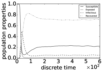
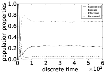
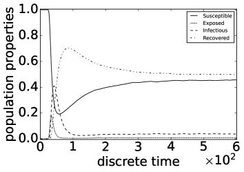
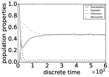
Figure 2: Population properties of one run of the simulation on two contact networks in Table 2. The first row is for Facebook and the second row is for Youtube. The left column uses the parameters $\beta=0.2,\sigma=1/3,\gamma=1/14,\rho=1/180$; the right column uses the parameters $\beta=0.27,\sigma=1/2,\gamma=1/7,\rho=1/90$.

From the point of view of filtering, a reasonable conjecture is that the rapid progress of the epidemic process in the first 50 to 100 steps will make it difficult to track the state distribution at the beginning of the epidemic. Furthermore, the slower pace of change after this point suggests that state tracking will then become easier. This conjecture is borne out by the experimental results that follow. The typical pattern in the applications is that the state errors of the filter are higher near the start of the epidemic, rising to a peak at around 30 time steps and then dropping to a lower, nearly constant, state error after about 100 steps. (The exact behaviour depends on the application, of course.) In applications where parameters have to be learned, there is a similar behaviour for the parameter errors. This is related to the fact that the accuracy of parameter estimation depends significantly on the accuracy of state tracking. It is necessary to be able to track the state accurately when the epidemic process parameters are known before attempting to simultaneously estimate the parameters and track the state.

3.5 Evaluating the Performance of Filters

This subsection presents the metrics that are used to evaluate the performance of the filters studied in this paper.

The first issue is how well a filter tracks the state. Consider first the nonconditional case. Suppose that $Y$ is the state space for both the simulation and the filter. Also suppose that $\widetilde{y}_{n}\in Y$ is the ground truth state at time $n$ given by the simulation. (Strictly, $\widetilde{y}:\Omega\rightarrow Y^{\mathbb{N}_{0}}$ is a stochastic process, so that each $\widetilde{y}_{n}:\Omega\rightarrow Y$ is a random variable.) Let $(\mu_{n}:H_{n}\rightarrow\mathcal{P}(Y))_{n\in\mathbb{N}_{0}}$ be the relevant schema so that $\mu_{n}(h_{n}):\mathcal{P}(Y)$ is the empirical belief at time $n$. Let $\savestack{\tmpbox}{\stretchto{\scaleto{\scalerel*[width("\mu_{n}(h_{n})")]{\kern-0.6pt\bigwedge\kern-0.6pt}{\rule[-614.295pt]{4.30554pt}{614.295pt}}}{}}{0.5ex}}\stackon[1pt]{\mu_{n}(h_{n})}{\tmpbox}:\mathcal{P}(Y)$ be the approximation of $\mu_{n}(h_{n})$ given by the filter at time $n$. Intuitively, we need a suitable measure of the ‘distance’ between the state $\widetilde{y}_{n}\in Y$ and the distribution $\savestack{\tmpbox}{\stretchto{\scaleto{\scalerel*[width("\mu_{n}(h_{n})")]{\kern-0.6pt\bigwedge\kern-0.6pt}{\rule[-614.295pt]{4.30554pt}{614.295pt}}}{}}{0.5ex}}\stackon[1pt]{\mu_{n}(h_{n})}{\tmpbox}\in\mathcal{P}(Y)$. Let $\rho:Y\times Y\rightarrow\mathbb{R}$ be a metric on $Y$. Then let

$$\mathit{Err}(\savestack{\tmpbox}{\stretchto{\scaleto{\scalerel*[width("\mu_{n}(h_{n})")]{\kern-0.6pt\bigwedge\kern-0.6pt}{\rule[-614.295pt]{4.30554pt}{614.295pt}}}{}}{0.5ex}}\stackon[1pt]{\mu_{n}(h_{n})}{\tmpbox})\triangleq\int_{Y}\lambda y.\rho(\widetilde{y}_{n},y)\;d\savestack{\tmpbox}{\stretchto{\scaleto{\scalerel*[width("\mu_{n}(h_{n})")]{\kern-0.6pt\bigwedge\kern-0.6pt}{\rule[-614.295pt]{4.30554pt}{614.295pt}}}{}}{0.5ex}}\stackon[1pt]{\mu_{n}(h_{n})}{\tmpbox}.$$ (12)

Thus $\mathit{Err}(\savestack{\tmpbox}{\stretchto{\scaleto{\scalerel*[width("\mu_{n}(h_{n})")]{\kern-0.6pt\bigwedge\kern-0.6pt}{\rule[-614.295pt]{4.30554pt}{614.295pt}}}{}}{0.5ex}}\stackon[1pt]{\mu_{n}(h_{n})}{\tmpbox})$ is a random variable whose value is the average error using the metric $\rho$ with respect to the filter’s estimate $\savestack{\tmpbox}{\stretchto{\scaleto{\scalerel*[width("\mu_{n}(h_{n})")]{\kern-0.6pt\bigwedge\kern-0.6pt}{\rule[-614.295pt]{4.30554pt}{614.295pt}}}{}}{0.5ex}}\stackon[1pt]{\mu_{n}(h_{n})}{\tmpbox}$ of the ground truth state $\widetilde{y}_{n}$ at time $n$.

For the conditional case, there is a schema $(\nu_{n}:H_{n}\rightarrow\mathcal{P}(X))_{n\in\mathbb{N}_{0}}$ for parameters and a schema $(\mu_{n}:H_{n}\times X\rightarrow\mathcal{P}(Y))_{n\in\mathbb{N}_{0}}$ for states conditional on the parameters. It can be shown that $(\nu_{n}\odot\mu_{n}:H_{n}\rightarrow\mathcal{P}(Y))_{n\in\mathbb{N}_{0}}$ is a schema for states. Let $\savestack{\tmpbox}{\stretchto{\scaleto{\scalerel*[width("(\nu_{n}\odot\mu_{n})(h_{n})")]{\kern-0.6pt\bigwedge\kern-0.6pt}{\rule[-614.295pt]{4.30554pt}{614.295pt}}}{}}{0.5ex}}\stackon[1pt]{(\nu_{n}\odot\mu_{n})(h_{n})}{\tmpbox}\in\mathcal{P}(Y)$ be the approximation of $(\nu_{n}\odot\mu_{n})(h_{n})$ given by the filter at time $n$. In this case, let

$$\mathit{Err}((\savestack{\tmpbox}{\stretchto{\scaleto{\scalerel*[width("\nu_{n}\odot\mu_{n})(h_{n})")]{\kern-0.6pt\bigwedge\kern-0.6pt}{\rule[-614.295pt]{4.30554pt}{614.295pt}}}{}}{0.5ex}}\stackon[1pt]{\nu_{n}\odot\mu_{n})(h_{n})}{\tmpbox})\triangleq\int_{Y}\lambda y.\rho(\widetilde{y}_{n},y)\;d\savestack{\tmpbox}{\stretchto{\scaleto{\scalerel*[width("(\nu_{n}\odot\mu_{n})(h_{n})")]{\kern-0.6pt\bigwedge\kern-0.6pt}{\rule[-614.295pt]{4.30554pt}{614.295pt}}}{}}{0.5ex}}\stackon[1pt]{(\nu_{n}\odot\mu_{n})(h_{n})}{\tmpbox}.$$ (13)

Note that $\nu_{n}\odot\mu_{n}:H_{n}\rightarrow\mathcal{P}(Y)$ is the marginal probability kernel for $\nu_{n}\otimes\mu_{n}:H_{n}\rightarrow\mathcal{P}(X\times Y)$ with respect to $Y$. (The definition of $\otimes$ for probability measures is given by Lloyd (2022).) In both the nonconditional and conditional cases, the average is with respect to the filter’s estimate of the empirical belief on $Y$. Both $\mathit{Err}(\savestack{\tmpbox}{\stretchto{\scaleto{\scalerel*[width("\mu_{n}(h_{n})")]{\kern-0.6pt\bigwedge\kern-0.6pt}{\rule[-614.295pt]{4.30554pt}{614.295pt}}}{}}{0.5ex}}\stackon[1pt]{\mu_{n}(h_{n})}{\tmpbox})$ and $\mathit{Err}(\savestack{\tmpbox}{\stretchto{\scaleto{\scalerel*[width("(\nu_{n}\odot\mu_{n})(h_{n})")]{\kern-0.6pt\bigwedge\kern-0.6pt}{\rule[-614.295pt]{4.30554pt}{614.295pt}}}{}}{0.5ex}}\stackon[1pt]{(\nu_{n}\odot\mu_{n})(h_{n})}{\tmpbox})$ are referred to as the state error (at time $n$).

An alternative approach to the above is to identify the ground truth state with the Dirac measure at that state. In this case, we require instead the definition of a distance between probability measures. The most natural definition of such a distance is the total variation metric that produces a value in the range $[0,1]$. However only in exceptional circumstances is the total variation metric computable, although it may be possible in some applications to compute reasonably accurate bounds on the value of this metric. This approach is not pursued here. Also note that there is a fundamental difference between the simulation case considered here and a similar problem of defining a metric that arises in convergence theorems for filters. For convergence theorems, one also requires a metric that defines the distance between two probability measures. One is the conditional probability defined by the underlying stochastic process of the state distribution given a particular history. The other is the approximation of this distribution for the same history given by the filtering algorithm employed. In this case, the total variation metric is a natural metric for defining the distance between these two probability measures, but the fact that this metric is not computable is of little consequence for convergence theorems.

Often $Y$ is a product space $\prod_{l=1}^{p}Y_{l}$. In this case, let $\rho_{l}:Y_{l}\times Y_{l}\rightarrow\mathbb{R}$ be a metric on $Y_{l}$, for $l=1,\ldots,p$. Then the metric $\rho:\prod_{l=1}^{p}Y_{l}\times\prod_{l=1}^{p}Y_{l}\rightarrow\mathbb{R}$ can be defined by

$$\rho(y,z)=\frac{1}{p}\sum_{l=1}^{p}\rho_{l}(y_{l},z_{l}),$$

for all $y,z\in\prod_{l=1}^{p}Y_{l}$. The constant $1/p$ is introduced to make the error less dependent on the size of the dimension $p$. Of course, there are many other ways of defining $\rho$ that could be used instead – the definition here is convenient for our purpose. Suppose now that $\savestack{\tmpbox}{\stretchto{\scaleto{\scalerel*[width("\mu_{n}(h_{n})")]{\kern-0.6pt\bigwedge\kern-0.6pt}{\rule[-614.295pt]{4.30554pt}{614.295pt}}}{}}{0.5ex}}\stackon[1pt]{\mu_{n}(h_{n})}{\tmpbox}$ can be factorized so that $\savestack{\tmpbox}{\stretchto{\scaleto{\scalerel*[width("\mu_{n}(h_{n})")]{\kern-0.6pt\bigwedge\kern-0.6pt}{\rule[-614.295pt]{4.30554pt}{614.295pt}}}{}}{0.5ex}}\stackon[1pt]{\mu_{n}(h_{n})}{\tmpbox}=\bigotimes_{l=1}^{p}\savestack{\tmpbox}{\stretchto{\scaleto{\scalerel*[width("\mu_{n}^{(l)}(h_{n}^{(l)})")]{\kern-0.6pt\bigwedge\kern-0.6pt}{\rule[-614.295pt]{4.30554pt}{614.295pt}}}{}}{0.5ex}}\stackon[1pt]{\mu_{n}^{(l)}(h_{n}^{(l)})}{\tmpbox}$, where $\savestack{\tmpbox}{\stretchto{\scaleto{\scalerel*[width("\mu_{n}^{(l)}(h_{n}^{(l)})")]{\kern-0.6pt\bigwedge\kern-0.6pt}{\rule[-614.295pt]{4.30554pt}{614.295pt}}}{}}{0.5ex}}\stackon[1pt]{\mu_{n}^{(l)}(h_{n}^{(l)})}{\tmpbox}$ is an approximation of the empirical belief $\mu_{n}^{(l)}(h_{n}^{(l)})\in\mathcal{P}(Y_{l})$, for $l=1,\ldots,p$. Then

Thus

$$\mathit{Err}(\savestack{\tmpbox}{\stretchto{\scaleto{\scalerel*[width("\mu_{n}(h_{n})")]{\kern-0.6pt\bigwedge\kern-0.6pt}{\rule[-614.295pt]{4.30554pt}{614.295pt}}}{}}{0.5ex}}\stackon[1pt]{\mu_{n}(h_{n})}{\tmpbox})=\frac{1}{p}\sum_{l=1}^{p}\int_{Y_{l}}\lambda y^{(l)}.\rho_{l}(\widetilde{y}_{n}^{(l)},y^{(l)})\;d\savestack{\tmpbox}{\stretchto{\scaleto{\scalerel*[width("\mu_{n}^{(l)}(h_{n}^{(l)})")]{\kern-0.6pt\bigwedge\kern-0.6pt}{\rule[-614.295pt]{4.30554pt}{614.295pt}}}{}}{0.5ex}}\stackon[1pt]{\mu_{n}^{(l)}(h_{n}^{(l)})}{\tmpbox}.$$ (14)

Intuitively, $\mathit{Err}(\savestack{\tmpbox}{\stretchto{\scaleto{\scalerel*[width("\mu_{n}(h_{n})")]{\kern-0.6pt\bigwedge\kern-0.6pt}{\rule[-614.295pt]{4.30554pt}{614.295pt}}}{}}{0.5ex}}\stackon[1pt]{\mu_{n}(h_{n})}{\tmpbox})$ is a random variable whose value is the average over all $p$ clusters of the average error using the metric $\rho_{l}$ with respect to the filter’s estimate $\savestack{\tmpbox}{\stretchto{\scaleto{\scalerel*[width("\mu_{n}^{(l)}(h_{n}^{(l)})")]{\kern-0.6pt\bigwedge\kern-0.6pt}{\rule[-614.295pt]{4.30554pt}{614.295pt}}}{}}{0.5ex}}\stackon[1pt]{\mu_{n}^{(l)}(h_{n}^{(l)})}{\tmpbox}$ of the $l$th component $\widetilde{y}_{n}^{(l)}$ of the ground truth state at time $n$. There is an analogous expression for the conditional case.

In the applications considered here, the state space is either $C^{L}$ or $S^{L}$. For the first case, a metric on $C$ is needed and for this purpose the discrete metric is the obvious choice. In this case, the state error is bounded above by $1$. For $S$, the metric $d:S\times S\rightarrow\mathbb{R}$ defined by $d(x,y)=\sum_{j=1}^{4}|x_{j}-y_{j}|$, for all $x,y\in S$, where $x_{4}\triangleq 1-\sum_{i=1}^{3}x_{i}$ and $y_{4}\triangleq 1-\sum_{i=1}^{3}y_{i}$, is employed. The definition of the metric is independent of the choice of fill-up argument. In this case, the state error is bounded above by $2$.

The second issue is how well the filter learns the parameters of the simulation. Let $X=\prod_{j=1}^{k}X_{j}=\mathbb{R}^{k}$, for some $k\geq 1$, and $\widetilde{x}=(\widetilde{x}_{1},\ldots,\widetilde{x}_{k})$ be the ground truth parameter value. Let

$$\mathit{Err}_{j}(\savestack{\tmpbox}{\stretchto{\scaleto{\scalerel*[width("\nu_{n}(h_{n})")]{\kern-0.6pt\bigwedge\kern-0.6pt}{\rule[-614.295pt]{4.30554pt}{614.295pt}}}{}}{0.5ex}}\stackon[1pt]{\nu_{n}(h_{n})}{\tmpbox})\triangleq\frac{1}{\widetilde{x}_{j}}\int_{X}\lambda x.|\widetilde{x}_{j}-x_{j}|\;d\savestack{\tmpbox}{\stretchto{\scaleto{\scalerel*[width("\nu_{n}(h_{n})")]{\kern-0.6pt\bigwedge\kern-0.6pt}{\rule[-614.295pt]{4.30554pt}{614.295pt}}}{}}{0.5ex}}\stackon[1pt]{\nu_{n}(h_{n})}{\tmpbox},$$ (15)

for $j=1,\ldots,k$. Thus $\mathit{Err}_{j}(\savestack{\tmpbox}{\stretchto{\scaleto{\scalerel*[width("\nu_{n}(h_{n})")]{\kern-0.6pt\bigwedge\kern-0.6pt}{\rule[-614.295pt]{4.30554pt}{614.295pt}}}{}}{0.5ex}}\stackon[1pt]{\nu_{n}(h_{n})}{\tmpbox})$ is a random variable whose value is the average normalized absolute error with respect to the filter’s estimate $\savestack{\tmpbox}{\stretchto{\scaleto{\scalerel*[width("\nu_{n}(h_{n})")]{\kern-0.6pt\bigwedge\kern-0.6pt}{\rule[-614.295pt]{4.30554pt}{614.295pt}}}{}}{0.5ex}}\stackon[1pt]{\nu_{n}(h_{n})}{\tmpbox}$ of the ground truth parameter (component) $\widetilde{x}_{j}$ at time $n$, for $j=1,\ldots,k$. $\mathit{Err}_{j}(\savestack{\tmpbox}{\stretchto{\scaleto{\scalerel*[width("\nu_{n}(h_{n})")]{\kern-0.6pt\bigwedge\kern-0.6pt}{\rule[-614.295pt]{4.30554pt}{614.295pt}}}{}}{0.5ex}}\stackon[1pt]{\nu_{n}(h_{n})}{\tmpbox})$ is referred to as the $j$th parameter error (at time $n$).

In all the applications in this paper, the filter for the parameters is a particle filter. Suppose that $(x^{(i)}_{n})_{i=1}^{N}$ is the parameter particle family at time $n$. Thus $\savestack{\tmpbox}{\stretchto{\scaleto{\scalerel*[width("\nu_{n}(h_{n})")]{\kern-0.6pt\bigwedge\kern-0.6pt}{\rule[-614.295pt]{4.30554pt}{614.295pt}}}{}}{0.5ex}}\stackon[1pt]{\nu_{n}(h_{n})}{\tmpbox}=\frac{1}{N}\sum_{i=1}^{N}\delta_{x^{(i)}_{n}}$ and hence

$$\mathit{Err}_{j}(\savestack{\tmpbox}{\stretchto{\scaleto{\scalerel*[width("\nu_{n}(h_{n})")]{\kern-0.6pt\bigwedge\kern-0.6pt}{\rule[-614.295pt]{4.30554pt}{614.295pt}}}{}}{0.5ex}}\stackon[1pt]{\nu_{n}(h_{n})}{\tmpbox})=\frac{1}{\widetilde{x}_{j}}\frac{1}{N}\sum_{i=1}^{N}|\widetilde{x}_{j}-x^{(i)}_{n,j}|,$$ (16)

for $j=1,\ldots,k$. The $j$th parameter estimate (at time $n$), for $j=1,\ldots,k$, is given by

$$\frac{1}{N}\sum_{i=1}^{N}x_{n,j}^{(i)}.$$ (17)

4 Factored Filters for Epidemic Processes

Consider an epidemic process spreading on a contact network, as described in Section 3. Knowledge of the states and parameters of the epidemic process are crucial to understand how an infectious disease spreads in the population, which may enable effective containment measures.

In this section, we consider the problem of tracking epidemic processes on contact networks. (Estimating parameters is studied in Section 5.) For this kind of application, factored filters are appropriate since epidemic processes satisfy the requirements discussed in Subsection 2.4 which ensure that the factored filter gives a good approximation of the state distribution even for very large contact networks. The key characteristic of epidemics that can be exploited by the factored filter is the sparseness of contact networks. People become infected in an epidemic by the infectious people that they come into sufficiently close contact with. But whether people live in very large cities or small towns, in most circumstances, they have similar-sized sets of contacts that are usually quite small. This sparseness of contact networks translates into transition models that only depend on the small number of neighbours of a node; hence the resulting state distributions are likely to be approximately factorizable into independent factors.

This sparseness of contact networks is reflected in the datasets of Table 2 that we use. For example, the average node degree for the Youtube network is about 6. Thus the factored algorithm works well on this network, even though it has over 1M nodes. Similarly, the Facebook and GitHub networks each have average node degree about 15. This sparseness property is also likely to hold more generally in geophysical applications.

We empirically evaluate factored filtering given by each of the Algorithm 7, 8, and 9 for tracking epidemics transmitted through the SEIRS model on (mostly) large contact networks. The parameters are assumed to be known. Factored filtering for the state space is fully factored, where each cluster consists of a single node. We consider a factored filter, a factored particle filter, and a factored variational filter in turn.

4.1 Factored Filter

For this application, the state space for the simulation is $C^{L}$, where $C=\{\mathsf{S},\mathsf{E},\mathsf{I},\mathsf{R}\}$ and the observation space is $O=\{\texttt{+},\texttt{-},\texttt{?}\}$. The simulation uses the transition model given by Eq. (3) (together with Eq. (2), of course), and the observation model at each node is given by Eq. (8). Patient zero, having compartment $\mathsf{E}$, that is, it is exposed, is chosen uniformly at random to start the simulation. All other nodes initially have compartment $\mathsf{S}$, that is, they are susceptible.

The factored filter is Algorithm 7 and is fully factored for this application; thus each cluster is a single node. The transition and observation models for the filter are the same as for the simulation. The parameters are assumed to be known. The initial state distribution for the filter is as follows. Let $n_{0}$ be patient zero. Also let $(p_{1},p_{2},p_{3},p_{4})$ denote the tuple of probabilities for the compartments, in the order $\mathsf{S},\mathsf{E},\mathsf{I},\mathsf{R}$, for a node. Then the initial state distribution for the filter is

• $(0.29,0.4,0.3,0.01)$, for node $n_{0}$,

• $(0.49,0.3,0.2,0.01)$, for the neighbours of node $n_{0}$ (i.e., nodes that are 1 step away from $n_{0}$),

• $(0.69,0.2,0.1,0.01)$, for nodes that are 2 steps away from $n_{0}$, and

• $(0.97,0.01,0.01,0.01)$, for nodes that are 3 or more steps away from $n_{0}$.

For this application, there are simple closed-form expressions for the transition and observation updates that the filter can exploit. Here are the details for the filter.

Transition update

The transition model is defined using the function $\breve{\tau}_{n}^{(k)}:C^{L}\rightarrow\mathcal{D}(C)$, at each node $k$ and at each time $n$, whose definition is given by Eq. (3), as explained in Section 3. For node $k$ and time $n$, the intermediate distribution at node $k$ given by the transition update is

$$\breve{\overline{\mu}}_{n+1}^{(k)}(h_{n}^{(k)})\triangleq\lambda c.\int_{C^{L}}\lambda s.\breve{\tau}_{n+1}^{(k)}(s)(c)\;\bigotimes_{k^{\prime}=1}^{L}\breve{\mu}_{n}^{(k^{\prime})}(h_{n}^{(k^{\prime})})\;d\upsilon_{C^{L}}.$$

Since the underlying measure $\upsilon_{C^{L}}$ on $C^{L}$ is counting measure, this reduces to

$$\breve{\overline{\mu}}_{n+1}^{(k)}(h_{n}^{(k)})\triangleq\lambda c.\sum_{s\in C^{L}}\breve{\tau}_{n+1}^{(k)}(s)(c)\;\prod_{k^{\prime}=1}^{L}\breve{\mu}_{n}^{(k^{\prime})}(h_{n}^{(k^{\prime})})(s_{k^{\prime}}).$$

Then it can be shown that the intermediate distribution resulting from the transition update is as follows.

$$\breve{\overline{\mu}}_{n+1}^{(k)}(h_{n}^{(k)})(\mathsf{S})=\rho\,\breve{\mu}_{n}^{(k)}(h_{n}^{(k)})(\mathsf{R})+\left(\textstyle\prod_{l\in\mathcal{N}_{k}}(1-\beta\breve{\mu}_{n}^{(l)}(h_{n}^{(l)})(\mathsf{I}))\right)\breve{\mu}_{n}^{(k)}(h_{n}^{(k)})(\mathsf{S}),$$ (18)

$$\breve{\overline{\mu}}_{n+1}^{(k)}(h_{n}^{(k)})(\mathsf{E})=\left(1-\textstyle\prod_{l\in\mathcal{N}_{k}}(1-\beta\breve{\mu}_{n}^{(l)}(h_{n}^{(l)})(\mathsf{I}))\right)\breve{\mu}_{n}^{(k)}(h_{n}^{(k)})(\mathsf{S})+(1-\sigma)\,\breve{\mu}_{n}^{(k)}(h_{n}^{(k)})(\mathsf{E}),$$

$$\breve{\overline{\mu}}_{n+1}^{(k)}(h_{n}^{(k)})(\mathsf{I})=\sigma\,\breve{\mu}_{n}^{(k)}(h_{n}^{(k)})(\mathsf{E})+(1-\gamma)\,\breve{\mu}_{n}^{(k)}(h_{n}^{(k)})(\mathsf{I}),$$

$$\breve{\overline{\mu}}_{n+1}^{(k)}(h_{n}^{(k)})(\mathsf{R})=\gamma\,\breve{\mu}_{n}^{(k)}(h_{n}^{(k)})(\mathsf{I})+(1-\rho)\,\breve{\mu}_{n}^{(k)}(h_{n}^{(k)})(\mathsf{R}),$$

for all $n\in\mathbb{N}_{0}$ and $k=1,\dots,L$. In effect, Eq. (18) could be used to define directly the transition update without specifying the transition model.

As an example, here is the derivation of the expression for $\breve{\overline{\mu}}_{n+1}^{(k)}(h_{n}^{(k)})(\mathsf{S})$. Let $r_{1},\ldots,r_{q}$ be the indices of the nodes that are the neighbours of node $k$, so that $\mathcal{N}_{k}=\{r_{1},\ldots,r_{q}\}$. Then

$$\;\breve{\overline{\mu}}_{n+1}^{(k)}(h_{n}^{(k)})(\mathsf{S})$$

$$= \;\sum_{s\in C^{L}}\breve{\tau}_{n+1}^{(k)}(s)(\mathsf{S})\;\prod_{p=1}^{L}\breve{\mu}_{n}^{(p)}(h_{n}^{(p)})(s_{p})$$

$$= \;\sum_{\begin{subarray}{c}s\in C^{L}\\ s_{k}=\mathsf{R}\end{subarray}}\breve{\tau}_{n+1}^{(k)}(s)(\mathsf{S})\;\prod_{p=1}^{L}\breve{\mu}_{n}^{(p)}(h_{n}^{(p)})(s_{p})+\sum_{\begin{subarray}{c}s\in C^{L}\\ s_{k}=\mathsf{S}\end{subarray}}\breve{\tau}_{n+1}^{(k)}(s)(\mathsf{S})\;\prod_{p=1}^{L}\breve{\mu}_{n}^{(p)}(h_{n}^{(p)})(s_{p})$$

$$= \;\rho\sum_{\begin{subarray}{c}s\in C^{L}\\ s_{k}=\mathsf{R}\end{subarray}}\prod_{p=1}^{L}\breve{\mu}_{n}^{(p)}(h_{n}^{(p)})(s_{p})+\sum_{\begin{subarray}{c}s\in C^{L}\\ s_{k}=\mathsf{S}\end{subarray}}\breve{\tau}_{n+1}^{(k)}(s)(\mathsf{S})\;\prod_{p=1}^{L}\breve{\mu}_{n}^{(p)}(h_{n}^{(p)})(s_{p})$$

$$= \;\rho\,\breve{\mu}_{n}^{(k)}(h_{n}^{(k)})(\mathsf{R})\,\sum_{\begin{subarray}{c}s\in C^{L}\\ s_{k}=\mathsf{R}\end{subarray}}\prod_{\begin{subarray}{c}p=1,\ldots,L\\ p\neq k\end{subarray}}\breve{\mu}_{n}^{(p)}(h_{n}^{(p)})(s_{p})+\sum_{\begin{subarray}{c}s\in C^{L}\\ s_{k}=\mathsf{S}\end{subarray}}\breve{\tau}_{n+1}^{(k)}(s)(\mathsf{S})\;\prod_{p=1}^{L}\breve{\mu}_{n}^{(p)}(h_{n}^{(p)})(s_{p})$$

$$= \;\rho\,\breve{\mu}_{n}^{(k)}(h_{n}^{(k)})(\mathsf{R})+\sum_{\begin{subarray}{c}s\in C^{L}\\ s_{k}=\mathsf{S}\end{subarray}}\breve{\tau}_{n+1}^{(k)}(s)(\mathsf{S})\;\prod_{p=1}^{L}\breve{\mu}_{n}^{(p)}(h_{n}^{(p)})(s_{p})$$

$$= \;\rho\,\breve{\mu}_{n}^{(k)}(h_{n}^{(k)})(\mathsf{R})+\sum_{\begin{subarray}{c}s\in C^{L}\\ s_{k}=\mathsf{S}\end{subarray}}(1-\beta)^{d_{k}(s)}\;\prod_{p=1}^{L}\breve{\mu}_{n}^{(p)}(h_{n}^{(p)})(s_{p})$$

$$= \;\rho\,\breve{\mu}_{n}^{(k)}(h_{n}^{(k)})(\mathsf{R})+\left(\sum_{\begin{subarray}{c}s\in C^{L}\\ s_{k}=\mathsf{S}\end{subarray}}(1-\beta)^{d_{k}(s)}\;\prod_{\begin{subarray}{c}p=1,\ldots,L\\ p\neq k\end{subarray}}\breve{\mu}_{n}^{(p)}(h_{n}^{(p)})(s_{p})\right)\,\breve{\mu}_{n}^{(k)}(h_{n}^{(k)})(\mathsf{S})$$

$$= \;\rho\,\breve{\mu}_{n}^{(k)}(h_{n}^{(k)})(\mathsf{R})+\left(\sum_{(c_{1},\ldots,c_{q})\in C^{|\mathcal{N}_{k}|}}(1-\beta)^{\sum_{l=1}^{q}\mathbb{I}(c_{l}=\mathsf{I})}\prod_{l=1}^{q}\breve{\mu}_{n}^{(r_{l})}(h_{n}^{(r_{l})})(c_{l})\right)\,\breve{\mu}_{n}^{(k)}(h_{n}^{(k)})(\mathsf{S})$$

$$= \;\rho\,\breve{\mu}_{n}^{(k)}(h_{n}^{(k)})(\mathsf{R})+\left(\sum_{(c_{1},\ldots,c_{q})\in C^{|\mathcal{N}_{k}|}}\prod_{l=1}^{q}(1-\beta)^{\mathbb{I}(c_{l}=\mathsf{I})}\,\breve{\mu}_{n}^{(r_{l})}(h_{n}^{(r_{l})})(c_{l})\right)\,\breve{\mu}_{n}^{(k)}(h_{n}^{(k)})(\mathsf{S})$$

$$= \;\rho\,\breve{\mu}_{n}^{(k)}(h_{n}^{(k)})(\mathsf{R})+\left(\prod_{l=1}^{q}\sum_{c_{l}\in C}(1-\beta)^{\mathbb{I}(c_{l}=\mathsf{I})}\,\breve{\mu}_{n}^{(r_{l})}(h_{n}^{(r_{l})})(c_{l})\right)\,\breve{\mu}_{n}^{(k)}(h_{n}^{(k)})(\mathsf{S})$$

$$= \;\rho\,\breve{\mu}_{n}^{(k)}(h_{n}^{(k)})(\mathsf{R})+\left(\prod_{l=1}^{q}(1-\beta\breve{\mu}_{n}^{(r_{l})}(h_{n}^{(r_{l})})(\mathsf{I}))\right)\,\breve{\mu}_{n}^{(k)}(h_{n}^{(k)})(\mathsf{S})$$

$$= \;\rho\,\breve{\mu}_{n}^{(k)}(h_{n}^{(k)})(\mathsf{R})+\left(\prod_{l\in\mathcal{N}_{k}}(1-\beta\breve{\mu}_{n}^{(l)}(h_{n}^{(l)})(\mathsf{I}))\right)\,\breve{\mu}_{n}^{(k)}(h_{n}^{(k)})(\mathsf{S}).$$ (19)

The derivations for the other compartments, $\mathsf{E}$, $\mathsf{I}$, and $\mathsf{R}$, are similar.

Observation update

For the observation update, let $o_{n+1}^{(k)}\in O_{k}$ be the testing outcome for node $k$ at time step $n+1$. Then

$$\breve{\mu}_{n+1}^{(k)}(h_{n+1}^{(k)})(c)=\frac{\breve{\xi}_{n+1}^{(k)}(c)(o_{n+1}^{(k)})\;\breve{\overline{\mu}}_{n+1}^{(k)}(h_{n}^{(k)})(c)}{\sum_{c^{\prime}\in C}\breve{\xi}_{n+1}^{(k)}(c^{\prime})(o_{n+1}^{(k)})\;\breve{\overline{\mu}}_{n+1}^{(k)}(h_{n}^{(k)})(c^{\prime})},$$ (20)

for all $n\in\mathbb{N}_{0}$ and $c\in C$. Note that Eq. (20) is a tractable expression that can be easily simplified to an explicit categorical distribution at each node.

Experimental setup

The spreading of epidemics is simulated over three of the contact networks, Gowalla, Youtube, and AS-733, in Table 2. Note that AS-733 is a dynamic contact network. It is assumed that the infection spreads in the contact network according to the SEIRS epidemic model (Eq. (3)), and in each simulation a node is chosen uniformly at random from the set of all nodes and made the exposed compartment (i.e., the patient zero), and all other nodes in the contact network are susceptible. Epidemics evolve following the transitions given by Eq. (3) for 600 time steps and generate observations according to Eq. (8) at each time step. In particular, we consider a testing method (for the observation model) which allows large-scale testing (about $20\%$ of the susceptible population, i.e., $\alpha_{\mathsf{S}}=0.2$) but may not be particularly accurate. The setup also assumes that most (about $90\%$, i.e., $\alpha_{\mathsf{I}}=0.9$) infectious individuals will be tested (e.g., due to symptoms), with good contact tracing that identifies the majority (about $70\%$, i.e., $\alpha_{\mathsf{E}}=0.7$) of latent infected cases, and that the testing results can be received within $24$ hours. We also assume a small proportion (about $5\%$, i.e., $\alpha_{\mathsf{R}}=0.05$) of the recovered population will be tested due to the risk of reinfection. In summary, the following values are used throughout the paper for Eq. (8):

$$\alpha_{\mathsf{S}}=0.2,\ \ \alpha_{\mathsf{E}}=0.7,\ \ \ \alpha_{\mathsf{I}}=0.9,\ \ \ \alpha_{\mathsf{R}}=0.05.$$ (21)

Two set of parameters corresponding to different infectious diseases are considered. Firstly, we consider an infection with transmission probability $\beta=0.2$ (i.e., transmission rate per day), the average pre-infectious period $\sigma^{-1}=3$ days, the average infectious period $\gamma^{-1}=14$ days, and the average period for immunity loss $\rho^{-1}=180$ days, i.e., an infectious disease similar to COVID-19 Gatto et al. (2020); Della Rossa et al. (2020); Cohen and Burbelo (2020); Lumley et al. (2021). Also we use a testing method with $\lambda_{FP}=\lambda_{FN}=0.1$ (i.e., false positive rate = false negative rate = $10\%$), which is similar to some rapid point-of-care testing for COVID-19 Dinnes et al. (2021). In summary,

$$\beta=0.2,\ \ \ \sigma=\frac{1}{3},\ \ \ \gamma=\frac{1}{14},\ \ \ \rho=\frac{1}{180},\ \ \ \lambda_{FP}=\lambda_{FN}=0.1.$$ (22)

Note that the average period of immunity loss is significantly longer than the average pre-infectious and infectious periods, i.e., $\rho$ is significantly smaller than $\sigma$ and $\gamma$.

Secondly, we consider an infection with transmission probability $\beta=0.27$, the average pre-infectious period $\sigma^{-1}=2$ days, the average infectious period $\gamma^{-1}=7$ days, and the average period for immunity loss $\rho^{-1}=90$ days, which imitate an infectious disease like one caused by an influenza A virus before effective vaccines are widely administered Yang et al. (2009); CDC (2019); Camacho et al. (2011); Slifka and Ahmed (1996). Also we use a testing method with $10\%$ false positive rate ($\lambda_{FP}=0.1$) and $30\%$ false negative rate ($\lambda_{FN}=0.3)$, which is comparable to many rapid influenza diagnostic tests that can be used in a physician’s office CDC (2020), and therefore widely random testing would be practical. Thus

$$\beta=0.27,\ \ \ \sigma=\frac{1}{2},\ \ \ \gamma=\frac{1}{7},\ \ \ \rho=\frac{1}{90},\ \ \ \lambda_{FP}=0.1,\ \ \ \lambda_{FN}=0.3.$$ (23)

Results and discussion

Epidemics are tracked using a fully factored version of the factored filter (Algorithm 7). To define the state error given by Eq. (12), we employ the metric $\rho:C^{L}\times C^{L}\rightarrow\mathbb{R}$ defined by

$$\rho(y,z)=\frac{1}{L}\sum_{k=1}^{L}\kappa(y_{k},z_{k}),$$

for all $y,z\in C^{L}$, where $\kappa:C\times C\rightarrow\mathbb{R}$ is the discrete metric. Thus the state error at time $n$ given by Eq. (14) is

$$K^{2}\left[\begin{array}[]{llll}\psi^{\prime}(K\gamma_{1})-\psi^{\prime}(\sum_{j=1}^{4}K\gamma_{j})&-\psi^{\prime}(\sum_{j=1}^{4}K\gamma_{j})&-\psi^{\prime}(\sum_{j=1}^{4}K\gamma_{j})&-\psi^{\prime}(\sum_{j=1}^{4}K\gamma_{j})\\[5.0pt] -\psi^{\prime}(\sum_{j=1}^{4}K\gamma_{j})&\psi^{\prime}(K\gamma_{2})-\psi^{\prime}(\sum_{j=1}^{4}K\gamma_{j})&-\psi^{\prime}(\sum_{j=1}^{4}K\gamma_{j})&-\psi^{\prime}(\sum_{j=1}^{4}K\gamma_{j})\\[5.0pt] -\psi^{\prime}(\sum_{j=1}^{4}K\gamma_{j})&-\psi^{\prime}(\sum_{j=1}^{4}K\gamma_{j})&\psi^{\prime}(K\gamma_{3})-\psi^{\prime}(\sum_{j=1}^{4}K\gamma_{j})&-\psi^{\prime}(\sum_{j=1}^{4}K\gamma_{j})\\[5.0pt] -\psi^{\prime}(\sum_{j=1}^{4}K\gamma_{j})&-\psi^{\prime}(\sum_{j=1}^{4}K\gamma_{j})&-\psi^{\prime}(\sum_{j=1}^{4}K\gamma_{j})&\psi^{\prime}(K\gamma_{4})-\psi^{\prime}(\sum_{j=1}^{4}K\gamma_{j})\end{array}\right],$$

where $\psi^{\prime}$ is the trigamma function.

According to Sylvester’s criterion, it is sufficient to show that each of the leading principal minors is positive. Now the leading principal minors are

$$\left|\begin{array}[]{ll}\psi^{\prime}(K\gamma_{1})-\psi^{\prime}(\sum_{j=1}^{4}K\gamma_{j})\\[5.0pt] \end{array}\right|$$

$$=\psi^{\prime}(K\gamma_{1})-\psi^{\prime}(\sum_{j=1}^{4}K\gamma_{j})$$

$$\left|\begin{array}[]{ll}\psi^{\prime}(K\gamma_{1})-\psi^{\prime}(\sum_{j=1}^{4}K\gamma_{j})&-\psi^{\prime}(\sum_{j=1}^{4}K\gamma_{j})\\[5.0pt] -\psi^{\prime}(\sum_{j=1}^{4}K\gamma_{j})&\psi^{\prime}(K\gamma_{2})-\psi^{\prime}(\sum_{j=1}^{4}K\gamma_{j})\\[5.0pt] \end{array}\right|$$

$$=\psi^{\prime}(K\gamma_{1})\psi^{\prime}(K\gamma_{2})-\psi^{\prime}(\sum_{j=1}^{4}K\gamma_{j})\left(\psi^{\prime}(K\gamma_{1})+\psi^{\prime}(K\gamma_{2})\right)$$

$$\left|\begin{array}[]{lll}\psi^{\prime}(K\gamma_{1})-\psi^{\prime}(\sum_{j=1}^{4}K\gamma_{j})&-\psi^{\prime}(\sum_{j=1}^{4}K\gamma_{j})&-\psi^{\prime}(\sum_{j=1}^{4}K\gamma_{j})\\[5.0pt] -\psi^{\prime}(\sum_{j=1}^{4}K\gamma_{j})&\psi^{\prime}(K\gamma_{2})-\psi^{\prime}(\sum_{j=1}^{4}K\gamma_{j})&-\psi^{\prime}(\sum_{j=1}^{4}K\gamma_{j})\\[5.0pt] -\psi^{\prime}(\sum_{j=1}^{4}K\gamma_{j})&-\psi^{\prime}(\sum_{j=1}^{4}K\gamma_{j})&\psi^{\prime}(K\gamma_{3})-\psi^{\prime}(\sum_{j=1}^{4}K\gamma_{j})\\[5.0pt] \end{array}\right|$$

$$=\psi^{\prime}(K\gamma_{1})\psi^{\prime}(K\gamma_{2})\psi^{\prime}(K\gamma_{3})-\psi^{\prime}(\sum_{j=1}^{4}K\gamma_{j})\left(\psi^{\prime}(K\gamma_{1})\psi^{\prime}(K\gamma_{2})+\psi^{\prime}(K\gamma_{1})\psi^{\prime}(K\gamma_{3})+\psi^{\prime}(K\gamma_{2})\psi^{\prime}(K\gamma_{3})\right)$$

$$\left|\begin{array}[]{llll}\psi^{\prime}(K\gamma_{1})-\psi^{\prime}(\sum_{j=1}^{4}K\gamma_{j})&-\psi^{\prime}(\sum_{j=1}^{4}K\gamma_{j})&-\psi^{\prime}(\sum_{j=1}^{4}K\gamma_{j})&-\psi^{\prime}(\sum_{j=1}^{4}K\gamma_{j})\\[5.0pt] -\psi^{\prime}(\sum_{j=1}^{4}K\gamma_{j})&\psi^{\prime}(K\gamma_{2})-\psi^{\prime}(\sum_{j=1}^{4}K\gamma_{j})&-\psi^{\prime}(\sum_{j=1}^{4}K\gamma_{j})&-\psi^{\prime}(\sum_{j=1}^{4}K\gamma_{j})\\[5.0pt] -\psi^{\prime}(\sum_{j=1}^{4}K\gamma_{j})&-\psi^{\prime}(\sum_{j=1}^{4}K\gamma_{j})&\psi^{\prime}(K\gamma_{3})-\psi^{\prime}(\sum_{j=1}^{4}K\gamma_{j})&-\psi^{\prime}(\sum_{j=1}^{4}K\gamma_{j})\\[5.0pt] -\psi^{\prime}(\sum_{j=1}^{4}K\gamma_{j})&-\psi^{\prime}(\sum_{j=1}^{4}K\gamma_{j})&-\psi^{\prime}(\sum_{j=1}^{4}K\gamma_{j})&\psi^{\prime}(K\gamma_{4})-\psi^{\prime}(\sum_{j=1}^{4}K\gamma_{j})\end{array}\right|$$

$$=\psi^{\prime}(K\gamma_{1})\psi^{\prime}(K\gamma_{2})\psi^{\prime}(K\gamma_{3})\psi^{\prime}(K\gamma_{4})\;-$$

$$\psi^{\prime}(\sum_{j=1}^{4}K\gamma_{j})\left(\psi^{\prime}(K\gamma_{1})\psi^{\prime}(K\gamma_{2})\psi^{\prime}(K\gamma_{3})+\psi^{\prime}(K\gamma_{1})\psi^{\prime}(K\gamma_{2})\psi^{\prime}(K\gamma_{4})+\psi^{\prime}(K\gamma_{1})\psi^{\prime}(K\gamma_{3})\psi^{\prime}(K\gamma_{4})\;+\right.$$

$$\hskip 250.00038pt\left.\psi^{\prime}(K\gamma_{2})\psi^{\prime}(K\gamma_{3})\psi^{\prime}(K\gamma_{4})\right).$$

The first leading principal minor is positive since $\psi^{\prime}$ is strictly decreasing on $\mathbb{R}_{+}$. For the other three cases, we will need the following result by Ronning (1986):

$$\psi^{\prime}(x)-\alpha\psi^{\prime}(\alpha x)<0,\ \text{for all $x>0$ and $0<\alpha<1$.}$$

For the third case,

$$\;\psi^{\prime}(K\gamma_{1})\psi^{\prime}(K\gamma_{2})\psi^{\prime}(K\gamma_{3})$$

$$= \;\frac{K\gamma_{1}}{\sum_{j=1}^{3}K\gamma_{j}}\psi^{\prime}(K\gamma_{1})\psi^{\prime}(K\gamma_{2})\psi^{\prime}(K\gamma_{3})+\frac{K\gamma_{2}}{\sum_{j=1}^{3}K\gamma_{j}}\psi^{\prime}(K\gamma_{1})\psi^{\prime}(K\gamma_{2})\psi^{\prime}(K\gamma_{3})+\frac{K\gamma_{3}}{\sum_{j=1}^{3}K\gamma_{j}}\psi^{\prime}(K\gamma_{1})\psi^{\prime}(K\gamma_{2})\psi^{\prime}(K\gamma_{3})$$

$$> \;\psi^{\prime}(\sum_{j=1}^{3}K\gamma_{j})\psi^{\prime}(K\gamma_{2})\psi^{\prime}(K\gamma_{3})+\psi^{\prime}(\sum_{j=1}^{3}K\gamma_{j})\psi^{\prime}(K\gamma_{1})\psi^{\prime}(K\gamma_{3})+\psi^{\prime}(\sum_{j=1}^{3}K\gamma_{j})\psi^{\prime}(K\gamma_{1})\psi^{\prime}(K\gamma_{2})\;\;\;\text{[\cite[cite]{\@@bibref{Authors Phrase1YearPhrase2}{Ronning:1986}{\@@citephrase{(}}{\@@citephrase{)}}}]}$$

$$> \;\psi^{\prime}(\sum_{j=1}^{4}K\gamma_{j})\left(\psi^{\prime}(K\gamma_{1})\psi^{\prime}(K\gamma_{2})+\psi^{\prime}(K\gamma_{1})\psi^{\prime}(K\gamma_{3})+\psi^{\prime}(K\gamma_{2})\psi^{\prime}(K\gamma_{3})\right).\;\;\;\;\;\text{[$\psi^{\prime}$ is strictly decreasing]}$$

The second and fourth cases are similar. Thus the objective function is convex.

Now setting the partial derivatives of $KL(p_{n}^{(k)}\|q_{n}^{(k)})+\lambda(\sum_{j=1}^{4}\gamma_{j}-1)$ equal to zero and adding the constraint $\sum_{j=1}^{4}\gamma_{j}-1=0$, we obtain the following equations

$$K\psi(K\gamma_{j})-K\psi(\sum_{j=1}^{4}K\gamma_{j})\;-$$

$$\hskip 10.00002ptM^{-1}\int_{S}\lambda y.\frac{\Gamma(\sum_{i=1}^{4}Cy_{i})}{\prod_{i=1}^{4}\Gamma(Cy_{i})}\prod_{i=1}^{4}o_{i}^{Cy_{i}-1}\;\mathit{Dir}(K\beta_{1}^{(k)},K\beta_{2}^{(k)},K\beta_{3}^{(k)},K\beta_{4}^{(k)})\;K\lambda y.\log y_{j}\;d\upsilon_{S}+\lambda=0,$$

$$\hskip 300.00046pt\text{ for }j=1,\ldots,4,$$

$$\sum_{j=1}^{4}\gamma_{j}-1=0.$$

Let

$$N_{j}\triangleq\int_{S}\lambda y.\frac{\Gamma(\sum_{i=1}^{4}Cy_{i})}{\prod_{i=1}^{4}\Gamma(Cy_{i})}\prod_{i=1}^{4}o_{i}^{Cy_{i}-1}\;\mathit{Dir}(K\beta_{1}^{(k)},K\beta_{2}^{(k)},K\beta_{3}^{(k)},K\beta_{4}^{(k)})\;K\lambda y.\log y_{j}\;d\upsilon_{S}$$

and $K_{j}\triangleq K\psi(K)+M^{-1}N_{j}$, for $j=1,\ldots,4$. Then the above set of equations becomes

$$\lambda=K_{j}-K\psi(K\gamma_{j}),\text{ for }j=1,\ldots,4,$$ (25)

$$\sum_{j=1}^{4}\gamma_{j}=1.$$

The constants $M$ and $N_{j}$, for $j=1,\ldots,4$, can be calculated using Monte Carlo integration by sampling from $\mathit{Dir}(K\beta_{1}^{(k)},K\beta_{2}^{(k)},K\beta_{3}^{(k)},K\beta_{4}^{(k)})$.

Since the system of equations in Eq. (25) does not appear to have a closed-form solution, we give an iterative algorithm that quickly finds accurate values for the $\gamma_{j}$. According to Eq. (25),

$$\sum_{j=1}^{4}\psi^{-1}(K^{-1}(K_{j}-\lambda))=K,$$ (26)

where $\psi^{-1}$ is the inverse digamma function. Using Eq. (26), we give an algorithm that provides an accurate approximation of $\lambda$, from which the $\gamma_{j}$ can be calculated.

The algorithm is a binary search algorithm. It starts with two values for $\lambda$, one for which $\sum_{j=1}^{4}\psi^{-1}(K^{-1}(K_{j}-\lambda))<K$ and one for which $\sum_{j=1}^{4}\psi^{-1}(K^{-1}(K_{j}-\lambda))>K$. Put

$$\lambda^{\prime}=\max_{j\in\{1,\ldots,4\}}\{K_{j}\}-K\psi(0.24K).$$

Then $\sum_{j=1}^{4}\psi^{-1}(K^{-1}(K_{j}-\lambda^{\prime}))<K$, since $\psi^{-1}$ is increasing. Now put

$$\lambda^{\prime\prime}=\min_{j\in\{1,\ldots,4\}}\{K_{j}\}-K\psi(0.26K).$$

Then $\sum_{j=1}^{4}\psi^{-1}(K^{-1}(K_{j}-\lambda^{\prime\prime}))>K$. Also $\lambda^{\prime\prime}<\lambda^{\prime}$.

The binary search algorithm is given in Algorithm 13. A suitable choice for $\varepsilon$ is $0.1$.

Algorithm 13 Equation Solver returns Approximate solution $\gamma_{1}$, $\gamma_{2}$, $\gamma_{3}$, $\gamma_{4}$ to Eq. (26) inputs: Constants $K_{1},K_{2},K_{3},K_{4}$,   initial values $\lambda^{\prime}=\max_{j\in\{1,\ldots,4\}}\{K_{j}\}-K\psi(0.24K)$ and   $\lambda^{\prime\prime}=\min_{j\in\{1,\ldots,4\}}\{K_{j}\}-K\psi(0.26K)$.

1:  while $\lambda^{\prime}-\lambda^{\prime\prime}\geq\varepsilon$ do

2:     $\lambda:=(\lambda^{\prime}+\lambda^{\prime\prime})/2$

3:     if $\sum_{j=1}^{4}\psi^{-1}(K^{-1}(K_{j}-\lambda))>K$ then

4:        $\lambda^{\prime\prime}:=\lambda$

5:     else

6:        $\lambda^{\prime}:=\lambda$

7:     end if

8:  end while

9:  $\lambda:=(\lambda^{\prime}+\lambda^{\prime\prime})/2$

10:  for $j=1$ to $4$ do

11:     $\gamma_{j}:=K^{-1}\psi^{-1}(K^{-1}(K_{j}-\lambda))$

12:  end for

13:  return  $\gamma_{1},\gamma_{2},\gamma_{3},\gamma_{4}$

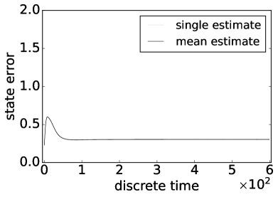
Figure 5: State errors of an SEIRS epidemic model for the contact network Facebook in Table 2 using Algorithm 9 for 100 independent runs in which the disease does not die out in 600 time steps. The left column uses the parameters $\beta=0.2,\sigma=1/3,\gamma=1/14,\rho=1/180$; the right column uses the parameters $\beta=0.27,\sigma=1/2,\gamma=1/7,\rho=1/90$. Light gray: state error from individual runs. Dark solid: mean state error averaged over 100 independent runs.

Figure 5 shows the results of tracking epidemics using Algorithm 9 for the contact network Facebook in Table 2. The parameter values are $K=10$ and $C=10$. The probability of a node being observed at a time step is $\alpha=0.5$. Because of the computational cost of this filtering algorithm, experiments were not carried out for larger contact networks.

5 Factored Conditional Filters for Epidemic Processes

We have shown how factored filters can exploit structure to accurately approximate state distributions for high-dimensional state spaces. This situation suggests that, when parameters also need to be estimated, it may be advantageous to employ factored conditional filters.

5.1 Factored Conditional Filter

We now evaluate factored conditional filtering in the setting of epidemics spreading on contact networks, in particular, we estimate the parameters in the SEIRS transition models (i.e., $\beta,\sigma,\gamma$, and $\rho$) and jointly track the states as the epidemics evolve over time. For this application, the state space for the simulation is $C^{L}$, where $C=\{\mathsf{S},\mathsf{E},\mathsf{I},\mathsf{R}\}$, the observation space is $O=\{\texttt{+},\texttt{-},\texttt{?}\}$, the transition model is given by Eq. (3), and the observation model at each node is given by Eq. (8).

The factored conditional filter (Algorithm 10) is employed for tracking states and the particle filter (Algorithm 2^∗) is employed for estimating parameters. The factored conditional filter is fully factored. The state space $Y$ for the filter is $C^{L}$, where $C=\{\mathsf{S},\mathsf{E},\mathsf{I},\mathsf{R}\}$ and the observation space is $O=\{\texttt{+},\texttt{-},\texttt{?}\}$. The transition model for $Y$ is given by Eq. (3) (with an extra argument for the parameter space $X$), and the observation model at each node is given by Eq. (8) (with an extra argument for the parameter space $X$). (See the signatures for the transition and observation models for the state space $Y$ in Section 2.3.) The parameter space $X$ is $[0,1]^{4}$. The transition model for the parameter space is a jittering transition model described below. The observation model for the parameter space can be computed as described in Section 2.3. In a similar way to Section 4.1, there are simple closed-form expressions for the transition and observation updates that the factored conditional filter can exploit.

For this application, the agent acquires two empirical beliefs: $\nu_{n}(h_{n}):\mathcal{P}(X)$, the parameter distribution at time $n$, and $\lambda x.\mu_{n}(h_{n},x):X\rightarrow\mathcal{P}(Y)$, the conditional state distribution given the parameters at time $n$. From these, the marginal state distribution $(\nu_{n}\odot\mu_{n})(h_{n})=\lambda A.\int_{X}\lambda x.\mu_{n}(h_{n},x)(A)\;d\nu_{n}(h_{n}):\mathcal{P}(Y)$ at time $n$ can be computed.

Note that Algorithm 2^∗ is a particle filter, while Algorithm 10 produces closed-form expressions. Together, the algorithms produce, for each parameter particle, a closed-form expression for the corresponding state distribution. So, strictly speaking, Algorithm 10 does not produce a conditional distribution but only an approximation of it restricted to a particular finite subset of parameter values.

The setup of experiments for the states is the same as in Section 4.1. The details for the parameters are as follows. A parameter particle filter with 300 particles is employed, so that $N=300$. The parameter particle family is initialized by sampling from uniform distributions as follows:

$$x^{(i)}_{0,1}\sim\mathcal{U}(0,0.8),\ \ \ x^{(i)}_{0,2}\sim\mathcal{U}(0,0.8),\ \ \ x^{(i)}_{0,3}\sim\mathcal{U}(0,0.8),\ \ \ x^{(i)}_{0,4}\sim\mathcal{U}(0,0.1),$$ (28)

where $i\in\{1,\dots,N\}$. An adaptive Gaussian jittering kernel is employed in Algorithm 2^∗ with covariance matrix

$$\Sigma_{n}=\max(ar^{n},b)\,\text{diag}(1,1,1,0.09),\ n\in\mathbb{N},$$ (29)

where $a=10^{-4},b=9\times 10^{-6},r=0.996$, and $\,\text{diag}(\cdot)$ is a diagonal matrix with the given diagonal entries. Parameter estimates are given by Eq. (17).

Figure 6 shows the results of tracking states, and Figures 7, 8, and 9 the results of estimating parameters using factored conditional filtering (Algorithms 10 and 2^∗). Compared with the results in Figure LABEL:fig:alg7 for Algorithm 7, not surprisingly, Algorithms 10 and 2^∗ have more difficulty tracking states at the beginning than Algorithm 7. However, by about 100 steps, Algorithms 10 and 2^∗ are tracking just as accurately as Algorithm 7. Furthermore, by around 150 steps, these algorithms are able to estimate the parameters accurately.

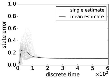
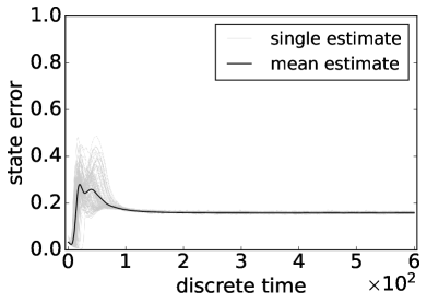
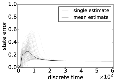
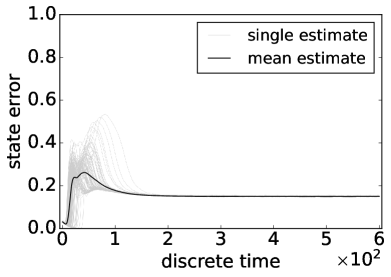
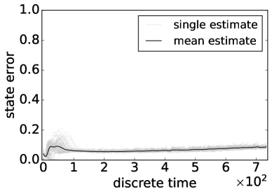
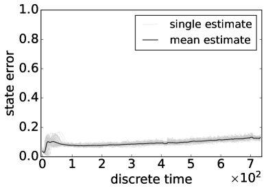
Figure 6: State errors of an SEIRS epidemic model for three contact networks in Table 2 using Algorithms 10 and 2^∗ for 100 independent runs in which the disease does not die out in 600 time steps for Gowalla and Youtube, and 733 time steps for AS-733. The first row is for Gowalla, the second row is for Youtube, and the third row is for AS-733. The left column uses the parameters $\beta=0.2,\sigma=1/3,\gamma=1/14,\rho=1/180,\lambda_{FP}=0.1,\lambda_{FN}=0.1$; the right column uses the parameters $\beta=0.27,\sigma=1/2,\gamma=1/7,\rho=1/90,\lambda_{FP}=0.1,\lambda_{FN}=0.3$. Light gray: state error from individual runs. Dark solid: mean state error averaged over 100 independent runs.

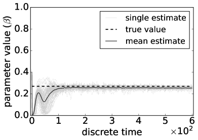
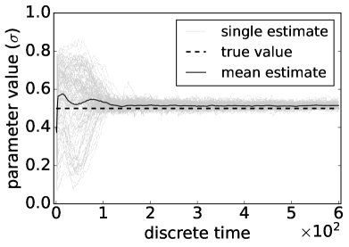
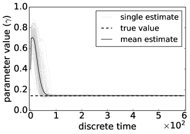
Figure 7: Parameter estimates of an SEIRS epidemic model for the Gowalla contact network using Algorithms 10 and 2^∗ for 100 independent runs in which the disease does not die out in 600 time steps. The parameters are $\beta=0.27,\sigma=1/2,\gamma=1/7,\rho=1/90,\lambda_{FP}=0.1,\lambda_{FN}=0.3$. Light gray: parameter estimate from individual runs. Dark solid: mean parameter estimate averaged over 100 independent runs.

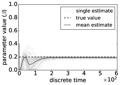
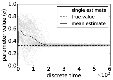
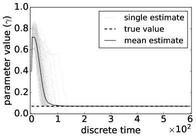
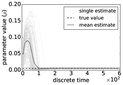
Figure 8: Parameter estimates of an SEIRS epidemic model for the Youtube contact network using Algorithms 10 and 2^∗ for 100 independent runs in which the disease does not die out in 600 time steps. The parameters are $\beta=0.2,\sigma=1/3,\gamma=1/14,\rho=1/180,\lambda_{FP}=0.1,\lambda_{FN}=0.1$. Light gray: parameter estimate from individual runs. Dark solid: mean parameter estimate averaged over 100 independent runs.

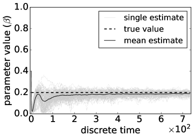
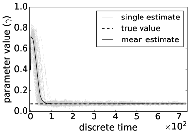
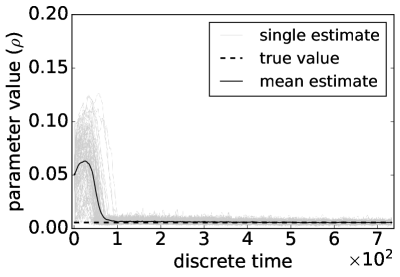
Figure 9: Parameter estimates of an SEIRS epidemic model for the AS-733 contact network using Algorithms 10 and 2^∗ for 100 independent runs in which the disease does not die out in 733 time steps. The parameters are $\beta=0.2,\sigma=1/3,\gamma=1/14,\rho=1/180,\lambda_{FP}=0.1,\lambda_{FN}=0.1$. Light gray: parameter estimate from individual runs. Dark solid: mean parameter estimate averaged over 100 independent runs.

5.2 Factored Conditional Particle Filter

Next we turn to Algorithm 11 which is the conditional version of Algorithm 8. This algorithm is fully factored and is used to estimate the parameters. Since it is a particle filter, the corresponding particle filter for the parameters is Algorithm 2^∗∗.

For this application, the state space for the simulation is $C^{L}$, where $C=\{\mathsf{S},\mathsf{E},\mathsf{I},\mathsf{R}\}$, the observation space is $O=\{\texttt{+},\texttt{-},\texttt{?}\}$, the transition model is given by Eq. (3), and the observation model at each node is given by Eq. (8). The state space $Y$ for the filter is $C^{L}$, where $C=\{\mathsf{S},\mathsf{E},\mathsf{I},\mathsf{R}\}$ and the observation space is $O=\{\texttt{+},\texttt{-},\texttt{?}\}$. The transition model for $Y$ is given by Eq. (3) (with an extra argument for the parameter space $X$), and the observation model at each node is given by Eq. (8) (with an extra argument for the parameter space $X$). (See the signatures for the transition and observation models for the state space $Y$ in Section 2.3.) The parameter space $X$ is $\mathbb{R}^{4}$. The transition model for the parameter space is a jittering transition model given in Eq. (29). The observation model for the parameter space can be computed as described in Section 2.3. There are $N=600$ parameter particles and $M=1024$ particles for the filters on each factor. The setup of experiments for the states is the same as in Section 4.1.

Figures 10 and 11 show the results of tracking states and estimating parameters using the factored conditional particle filtering (Algorithms 11 and 2^∗∗) for the parameter set in Eq. (23). We remark that Algorithm 11 is more computationally expensive and thus unlikely to scale to graphs as large as the Youtube Mislove et al. (2007). In addition, the performance for tracking states and estimating parameters using Algorithm 11 is less effective compared to that of Algorithm 10. Nevertheless, Algorithm 11 could be employed in settings where exact filtering as in Algorithm 10 is not applicable.

Figure 10: State errors of an SEIRS epidemic model for the OpenFlights contact network using Algorithms 11 and 2^∗∗ for 100 independent runs in which the disease does not die out in 600 time steps. The parameters are $\beta=0.27,\sigma=1/2,\gamma=1/7,\rho=1/90,\lambda_{FP}=0.1,\lambda_{FN}=0.3$. Light gray: state error from individual runs. Dark solid: mean state error averaged over 100 independent runs.

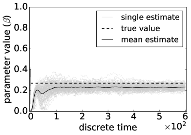
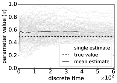
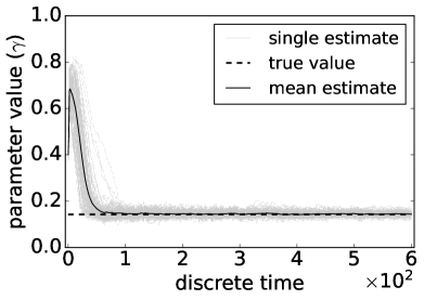
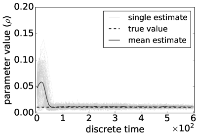
Figure 11: Parameter estimates of an SEIRS epidemic model for the OpenFlights contact network using Algorithms 11 and 2^∗∗ for 100 independent runs in which the disease does not die out in 600 time steps. The parameters are $\beta=0.27,\sigma=1/2,\gamma=1/7,\rho=1/90$. Light gray: parameter estimate from individual runs. Dark solid: parameter estimate averaged over 100 independent runs.

5.3 Factored Conditional Variational Filter

For the application of this subsection, the state space for the simulation is $S^{L}$ and the transition model is given by Eq. (6) (together with Eq. (5)), for $K=3$. The observation model is given by Eq. (11) with $m=5$. The probability of a node being observed at a time step is $\alpha=0.7$. Note that $\mathit{Mult}(m,(s_{1},s_{2},s_{3},s_{4}))$ in Eq. (11) can be written in the form

$$\lambda o.\frac{\Gamma(m+1)}{\prod_{j=1}^{4}\Gamma(o_{j}+1)}\prod_{j=1}^{4}s_{j}^{o_{j}}.$$

Now the filter is considered. The filtering algorithm is a fully factored version of the factored conditional variational filter (Algorithm 12). In a similar way to the application in Section LABEL:sec:FactoredVariationalFilter, instead of defining a transition model, a transition update is defined directly. Let $\mathcal{D}_{PD}(S^{L})$ be the set of all distributions on $S^{L}$ that are products of Dirichlet distributions on each factor $S$. The parameter space is $[0,1]^{4}$. For all $n\in\mathbb{N}$ and $k=1,\ldots,L$, define

$$\mathcal{T}_{n}^{(k)}:[0,1]^{4}\times\mathcal{D}_{PD}(S^{L})\rightarrow\mathcal{D}(S)$$

by

$$\mathcal{T}_{n}^{(k)}((\beta,\sigma,\gamma,\rho),\bigotimes_{k^{\prime}=1}^{L}\mathit{Dir}(\alpha_{1}^{(k^{\prime})},\alpha_{2}^{(k^{\prime})},\alpha_{3}^{(k^{\prime})},\alpha_{4}^{(k^{\prime})}))=\mathit{Dir}(K\beta_{1}^{(k)},K\beta_{2}^{(k)},K\beta_{3}^{(k)},K\beta_{4}^{(k)}),$$

where

$$\begin{aligned} &\beta_{1}^{(k)}\triangleq\rho\overline{\alpha}_{4}^{(k)}+\overline{i_{k}}\,\overline{i_{\mathcal{N}_{k}}}\overline{\alpha}_{1}^{(k)}\\ &\beta_{2}^{(k)}\triangleq(1-\overline{i_{k}}\,\overline{i_{\mathcal{N}_{k}}})\overline{\alpha}_{1}^{(k)}+(1-\sigma)\overline{\alpha}_{2}^{(k)}\\ &\beta_{3}^{(k)}\triangleq\sigma\overline{\alpha}_{2}^{(k)}+(1-\gamma)\overline{\alpha}_{3}^{(k)}\\ &\beta_{4}^{(k)}\triangleq\gamma\overline{\alpha}_{3}^{(k)}+(1-\rho)\overline{\alpha}_{4}^{(k)}\\ &\overline{i_{k}}\triangleq(1-\beta\kappa_{1}\overline{\alpha}_{3}^{(k)})^{M_{k}-1}\\ &\overline{i_{\mathcal{N}_{k}}}\triangleq\prod_{l\in\mathcal{N}_{k}}(1-\beta\kappa_{2}\overline{\alpha}_{3}^{(l)})^{M_{l}}\end{aligned}$$ (42)

and, for $k=1,\ldots,L$ and $j=1,\ldots,4$,

$$\overline{\alpha}_{j}^{(k)}\triangleq\frac{\alpha_{j}^{(k)}}{\sum_{i=1}^{4}\alpha_{i}^{(k)}}.$$

Then, for all $n\in\mathbb{N}$, the transition update $\mathcal{T}_{n}:[0,1]^{4}\times\mathcal{D}_{PD}(S^{L})\rightarrow\mathcal{D}_{PD}(S^{L})$ is given by

$$\mathcal{T}_{n}=\lambda(p,q).\bigotimes_{k=1}^{L}\mathcal{T}_{n}^{(k)}(p,q).$$

To understand Eq. (42), note that the transition model given by Eq. (6) contains a number of terms of the form $(1-\beta)^{M_{l}\kappa_{2}s_{l,3}}$ that reflects, on average, the probability that a susceptible individual $j_{k}$ remains uninfected by its neighbouring individuals. In the transition update, analogous to how Eq. (19) was derived, we need to consider the same event but probability-weighted by the number $n(j_{k})$ of infected neighbouring individuals connected to $j_{k}$, which is given by

$$\;\sum_{d=0}^{M_{l}}\Pr(n(j_{k})=d)(1-\beta)^{d}$$

$$= \;\sum_{d=0}^{M_{l}}\binom{M_{l}}{d}(\kappa_{2}\overline{\alpha}_{3}^{(l)})^{d}(1-\kappa_{2}\overline{\alpha}_{3}^{(l)})^{M_{l}-d}(1-\beta)^{d}$$

$$= \;((1-\kappa_{2}\overline{\alpha}_{3}^{(l)})+(1-\beta)\kappa_{2}\overline{\alpha}_{3}^{(l)})^{M_{l}}$$

$$= \;(1-\beta\kappa_{2}\overline{\alpha}_{3}^{(l)})^{M_{l}},$$

where the second-to-last line comes from the binomial theorem. The $(1-\beta)^{(M_{k}-1)\kappa_{1}s_{k,3}}$ term in Eq. (6) can be analysed in a similar way to yield $(1-\beta\kappa_{1}\overline{\alpha}_{3}^{(k)})^{M_{k}-1}$.

The observation model for the filter is given by Eq. (11) (applied at the subpopulation node level).

The details of the initializations, which are the same as in Section LABEL:sec:FactoredVariationalFilter, are as follows. (For subpopulation contact networks, the terminology ‘subpopulation zero’ is used instead of ‘patient zero’.) For the simulation, subpopulation zero, labelled by (0.01, 0.97, 0.01, 0.01), is chosen uniformly at random. All other nodes are initially labelled by (0.97, 0.01, 0.01, 0.01). For the filter, the initial state distribution is as follows. Let $n_{0}$ be subpopulation zero. Then the initial state distribution for the filter is given by the product of the Dirichlet distributions

• $\mathit{Dir}(0.29,0.4,0.3,0.01)$, for node $n_{0}$,

• $\mathit{Dir}(0.49,0.3,0.2,0.01)$, for the neighbours of node $n_{0}$,

• $\mathit{Dir}(0.69,0.2,0.1,0.01)$, for nodes that are 2 steps away from $n_{0}$, and

• $\mathit{Dir}(0.97,0.01,0.01,0.01)$, for nodes that are 3 or more steps away from $n_{0}$.

Now we consider the details of Algorithm 12 for this application. The transition update corresponding to Line 2 of Algorithm 12 is described above. For the observation update in Line 3, it is necessary to calculate, for $k=1,\ldots,L$,

$${p_{n}^{(k)}:=\lambda x.\frac{\lambda y.\breve{\xi}_{n}^{(k)}(y)(o_{n}^{(k)})\;\overline{q}_{n}^{(k)}(x)}{\int_{S}\lambda y.\breve{\xi}_{n}^{(k)}(y)(o_{n}^{(k)})\;\overline{q}_{n}^{(k)}(x)\;d\upsilon_{S}}}.$$

(Note that, in the following, it is only necessary to consider $x\in X$ that belong to the parameter particle family $(x_{n}^{(i)})_{i=1}^{N}$ at time $n$.) Suppose that

$$\overline{q}_{n}^{(k)}(x_{n}^{(i)})=\mathit{Dir}(K\beta_{1}^{(i,k)},K\beta_{2}^{(i,k)},K\beta_{3}^{(i,k)},K\beta_{4}^{(i,k)}),$$

for $i=1,\ldots,N$, and $o_{n}^{(k)}=(o_{1},o_{2},o_{3},o_{4})$. Hence, for $i=1,\ldots,N$,

$$\begin{aligned} &\;p_{n}^{(k)}(x_{n}^{(i)})\\ \propto&\;\lambda y.\breve{\xi}_{n}^{(k)}(y)(o_{n}^{(k)})\;\overline{q}_{n}^{(k)}(x_{n}^{(i)})\\ =&\;\lambda y.\frac{\Gamma(m+1)}{\prod_{j=1}^{4}\Gamma(o_{j}+1)}\prod_{j=1}^{4}y_{j}^{o_{j}}\;\mathit{Dir}(K\beta_{1}^{(i,k)},K\beta_{2}^{(i,k)},K\beta_{3}^{(i,k)},K\beta_{4}^{(i,k)})\\ =&\;\lambda y.\frac{\Gamma(m+1)}{\prod_{j=1}^{4}\Gamma(o_{j}+1)}\prod_{j=1}^{4}y_{j}^{o_{j}}\;\lambda y.\frac{\Gamma(\sum_{j=1}^{4}K\beta_{j}^{(i,k}))}{\prod_{j=1}^{4}\Gamma(K\beta_{j}^{(i,k)})}\prod_{j=1}^{4}y_{j}^{K\beta_{j}^{(i,k)}-1}\\ =&\;\lambda y.\frac{\Gamma(m+1)}{\prod_{j=1}^{4}\Gamma(o_{j}+1)}\;\frac{\Gamma(\sum_{j=1}^{4}K\beta_{j}^{(i,k)})}{\prod_{j=1}^{4}\Gamma(K\beta_{j}^{(i,k)})}\;\prod_{j=1}^{4}y_{j}^{o_{j}+K\beta_{j}^{(i,k)}-1}\\ =&\;\lambda y.\frac{\Gamma(m+1)}{\prod_{j=1}^{4}\Gamma(o_{j}+1)}\;\frac{\Gamma(K)}{\prod_{j=1}^{4}\Gamma(K\beta_{j}^{(i,k)})}\;\prod_{j=1}^{4}y_{j}^{o_{j}+K\beta_{j}^{(i,k)}-1}\hskip 40.00006pt\left[\sum_{j=1}^{4}\beta_{j}^{(i,k)}=1\right]\end{aligned}$$

Let $M_{i}\triangleq\int_{S}\lambda y.\frac{\Gamma(m+1)}{\prod_{j=1}^{4}\Gamma(o_{j}+1)}\;\frac{\Gamma(K)}{\prod_{j=1}^{4}\Gamma(K\beta_{j}^{(i,k)})}\;\;\prod_{j=1}^{4}y_{j}^{o_{j}+K\beta_{j}^{(i,k)}-1}\;d\upsilon_{S}$, for $i=1,\ldots,N$. Then, for $i=1,\ldots,N$,

$$M_{i}= \;\int_{S}\lambda y.\frac{\Gamma(m+1)}{\prod_{j=1}^{4}\Gamma(o_{j}+1)}\;\frac{\Gamma(K)}{\prod_{j=1}^{4}\Gamma(K\beta_{j}^{(i,k)})}\;\;\prod_{j=1}^{4}y_{j}^{o_{j}+K\beta_{j}^{(i,k)}-1}\;d\upsilon_{S}$$

$$= \;\frac{\Gamma(m+1)}{\prod_{j=1}^{4}\Gamma(o_{j}+1)}\;\frac{\Gamma(K)}{\prod_{j=1}^{4}\Gamma(K\beta_{j}^{(i,k)})}\;\frac{\prod_{j=1}^{k}\Gamma(o_{j}+K\beta_{j}^{(i,k)})}{\Gamma(m+K)}.$$

The next step is the variational update in Line 4 of Algorithm 12. Let $Q^{(k)}$ be the set of Dirichlet distributions on $S$, for $k=1,\ldots,L$. Then, for $k=1,\ldots,L$,

$$q_{n}^{(k)}= \;\operatorname*{argmin}_{q\in(Q^{(k)})^{X}}\int_{X}\lambda x.D_{\alpha}(p_{n}^{(k)}(x)\|q(x))\;d\nu_{n}(h_{n})$$

$$= \;\operatorname*{argmin}_{q\in(Q^{(k)})^{X}}\sum_{i=1}^{N}KL(p_{n}^{(k)}(x_{n}^{(i)})\|q(x_{n}^{(i)})).$$

It follows that $q_{n}^{(k)}:X\rightarrow Q^{(k)}$ is any function satisfying

$$q_{n}^{(k)}(x_{n}^{(i)})=\operatorname*{argmin}_{r\in Q^{(k)}}KL(p_{n}^{(k)}(x_{n}^{(i)})\|r),$$

for $i=1,\ldots,N$, and with arbitrary values for other $x\in X$. The issue now is to calculate

$$\operatorname*{argmin}_{r\in Q^{(k)}}KL(p_{n}^{(k)}(x_{n}^{(i)})\|r),$$

for $i=1,\ldots,N$.

Suppose that $r$ has the form $\mathit{Dir}(\gamma_{1}^{(i,k)},\gamma_{2}^{(i,k)},\gamma_{3}^{(i,k)},\gamma_{4}^{(i,k)})$. Then, for $i=1,\ldots,N$,

$$\;KL(p_{n}^{(k)}(x_{n}^{(i)})\|r)$$

$$= \;\int_{S}p_{n}^{(k)}(x_{n}^{(i)})\log\frac{p_{n}^{(k)}(x_{n}^{(i)})}{r}\;d\upsilon_{S}$$

$$= \;\int_{S}p_{n}^{(k)}(x_{n}^{(i)})\log\frac{p_{n}^{(k)}(x_{n}^{(i)})}{\mathit{Dir}(\gamma_{1}^{(i,k)},\gamma_{2}^{(i,k)},\gamma_{3}^{(i,k)},\gamma_{4}^{(i,k)})}\;d\upsilon_{S}$$

$$= \;\mathit{Const}-\int_{S}p_{n}^{(k)}(x_{n}^{(i)})\log\mathit{Dir}(\gamma_{1}^{(i,k)},\gamma_{2}^{(i,k)},\gamma_{3}^{(i,k)},\gamma_{4}^{(i,k)})\;d\upsilon_{S}$$

$$= \;\mathit{Const}-M_{i}^{-1}\int_{S}\lambda y.\frac{\Gamma(m+1)}{\prod_{j=1}^{4}\Gamma(o_{j}+1)}\;\frac{\Gamma(K)}{\prod_{j=1}^{4}\Gamma(K\beta_{j}^{(i,k)})}\prod_{j=1}^{4}y_{j}^{o_{j}+K\beta_{j}^{(i,k)}-1}$$

$$\hskip 230.00035pt\log\mathit{Dir}(\gamma_{1}^{(i,k)},\gamma_{2}^{(i,k)},\gamma_{3}^{(i,k)},\gamma_{4}^{(i,k)})\;d\upsilon_{S}$$

$$= \;\mathit{Const}-M_{i}^{-1}\int_{S}\lambda y.\frac{\Gamma(m+1)}{\prod_{j=1}^{4}\Gamma(o_{j}+1)}\;\frac{\Gamma(K)}{\prod_{j=1}^{4}\Gamma(K\beta_{j}^{(i,k)})}\;\prod_{j=1}^{4}y_{j}^{o_{j}+K\beta_{j}^{(i,k)}-1}$$

$$\hskip 90.00014pt\left(\log\Gamma(\sum_{j=1}^{4}\gamma_{j}^{(i,k)})-\log\prod_{j=1}^{4}\Gamma(\gamma_{j}^{(i,k)})+\lambda y.\sum_{j=1}^{4}(\gamma_{j}^{(i,k)}-1)\log y_{j}\right)\;d\upsilon_{S}$$

$$= \;\mathit{Const}-\left(\left(\log\Gamma(\sum_{j=1}^{4}\gamma_{j}^{(i,k)})-\log\prod_{j=1}^{4}\Gamma(\gamma_{j}^{(i,k)})\right)\;+\right.$$

$$\hskip 10.00002ptM_{i}^{-1}\int_{S}\lambda y.\frac{\Gamma(m+1)}{\prod_{j=1}^{4}\Gamma(o_{j}+1)}\;\frac{\Gamma(K)}{\prod_{j=1}^{4}\Gamma(K\beta_{j}^{(i,k)})}\;\prod_{j=1}^{4}y_{j}^{o_{j}+K\beta_{j}^{(i,k)}-1}\left.\lambda y.\sum_{j=1}^{4}(\gamma_{j}^{(i,k)}-1)\log y_{j}\;d\upsilon_{S}\right)$$

$$= \;\mathit{Const}-\left(\left(\log\Gamma(\sum_{j=1}^{4}\gamma_{j}^{(i,k)})-\log\prod_{j=1}^{4}\Gamma(\gamma_{j}^{(i,k)})\right)\;+\right.$$

$$\hskip 60.00009ptM_{i}^{-1}\frac{\Gamma(m+1)}{\prod_{j=1}^{4}\Gamma(o_{j}+1)}\;\frac{\Gamma(K)}{\prod_{j=1}^{4}\Gamma(K\beta_{j}^{(i,k)})}\;\frac{\prod_{j=1}^{4}\Gamma(o_{j}+K\beta_{j}^{(i,k)})}{\Gamma(m+K)}$$

$$\hskip 10.00002pt\left.\int_{S}\lambda y.\sum_{j=1}^{4}(\gamma_{j}^{(i,k)}-1)\log y_{j}\;\mathit{Dir}(o_{1}+K\beta_{1}^{(i,k)},o_{2}+K\beta_{2}^{(i,k)},o_{3}+K\beta_{3}^{(i,k)},o_{4}+K\beta_{4}^{(i,k)})\;d\upsilon_{S}\right)$$

$$= \;\mathit{Const}-\left(\left(\log\Gamma(\sum_{j=1}^{4}\gamma_{j}^{(i,k)})-\log\prod_{j=1}^{4}\Gamma(\gamma_{j}^{(i,k)})\right)\;+\right.$$

$$\hskip 60.00009ptM_{i}^{-1}\frac{\Gamma(m+1)}{\prod_{j=1}^{4}\Gamma(o_{j}+1)}\;\frac{\Gamma(K)}{\prod_{j=1}^{4}\Gamma(K\beta_{j}^{(i,k)})}\;\frac{\prod_{j=1}^{4}\Gamma(o_{j}+K\beta_{j}^{(i,k)})}{\Gamma(m+K)}$$

$$\hskip 100.00015pt\left.\sum_{j=1}^{4}(\gamma_{j}^{(i,k)}-1)(\psi(o_{j}+K\beta_{j}^{(i,k)})-\psi(\sum_{p=1}^{4}(o_{p}+K\beta_{p}^{(i,k)}))\right)$$

$$= \;\mathit{Const}-\left(\left(\log\Gamma(\sum_{j=1}^{4}\gamma_{j}^{(i,k)})-\log\prod_{j=1}^{4}\Gamma(\gamma_{j}^{(i,k)})\right)\;+\right.$$

$$\hskip 60.00009ptM_{i}^{-1}M_{i}\left.\sum_{j=1}^{4}(\gamma_{j}^{(i,k)}-1)(\psi(o_{j}+K\beta_{j}^{(i,k)})-\psi(m+K))\right)$$

$$= \;\mathit{Const}-\left(\left(\log\Gamma(\sum_{j=1}^{4}\gamma_{j}^{(i,k)})-\log\prod_{j=1}^{4}\Gamma(\gamma_{j}^{(i,k)})\right)\;+\right.$$

$$\hskip 150.00023pt\left.\sum_{j=1}^{4}(\gamma_{j}^{(i,k)}-1)(\psi(o_{j}+K\beta_{j}^{(i,k)}-\psi(m+K))\right),$$

where $\psi$ is the digamma function.

Let $f\triangleq\lambda(\gamma_{1}^{(i,k)},\gamma_{2}^{(i,k)},\gamma_{3}^{(i,k)},\gamma_{4}^{(i,k)}).KL(p_{n}^{(k)}(x_{n}^{(i)})\|r):\mathbb{R}_{+}^{4}\rightarrow\mathbb{R}$. The partial derivatives $D_{j}f$ of $f$ exist at each point $(\gamma_{1}^{(i,k)},\gamma_{2}^{(i,k)},\gamma_{3}^{(i,k)},\gamma_{4}^{(i,k)})\in\mathbb{R}_{+}^{4}$ and

$$D_{j}f(\gamma_{1}^{(i,k)},\gamma_{2}^{(i,k)},\gamma_{3}^{(i,k)},\gamma_{4}^{(i,k)})=\psi(\gamma_{j}^{(i,k)})-\psi(\sum_{j=1}^{4}\gamma_{j}^{(i,k)})-(\psi(o_{j}+K\beta_{j}^{(i,k)})-\psi(m+K)),$$

for $j=1,\ldots,4$. Thus, for $j=1,\ldots,4$,

$$D_{j}f(o_{1}+K\beta_{1}^{(i,k)},\ldots,o_{4}+K\beta_{4}^{(i,k)})=0.$$

Furthermore, the Hessian matrix of $f$ has the same form as the Hessian matrix in Section LABEL:sec:FactoredVariationalFilter and so is positive definite. Consequently, $f$ is a convex function and has a (global) minimum at $(o_{1}+K\beta_{1}^{(i,k)},\ldots,o_{4}+K\beta_{4}^{(i,k)})$. In summary,

$$q_{n}^{(k)}(x_{n}^{(i)})=\mathit{Dir}(o_{1}+K\beta_{1}^{(i,k)},\ldots,o_{4}+K\beta_{4}^{(i,k)}),$$

for $i=1,\ldots,N$. Since it is only necessary to consider $x\in X$ that belong to the parameter particle family $(x_{n}^{(i)})_{i=1}^{N}$, these equations provide a simple and efficient computation of $q_{n}^{(k)}$ in Line 4 of Algorithm 12.

Here is the formula for the state error $\mathit{Err}(\savestack{\tmpbox}{\stretchto{\scaleto{\scalerel*[width("(\nu_{n}\odot\mu_{n})(h_{n})")]{\kern-0.6pt\bigwedge\kern-0.6pt}{\rule[-614.295pt]{4.30554pt}{614.295pt}}}{}}{0.5ex}}\stackon[1pt]{(\nu_{n}\odot\mu_{n})(h_{n})}{\tmpbox})$:

In the derivation above, $\widetilde{y}_{n}^{(k)}=(\widetilde{y}_{n,1}^{(k)},\widetilde{y}_{n,2}^{(k)},\widetilde{y}_{n,3}^{(k)})$ is the ground truth state for the factor $k$ at time $n$ from the simulation, $\widetilde{y}_{n,4}^{(k)}\triangleq 1-\sum_{i=1}^{3}\widetilde{y}_{n,i}^{(k)}$, $y=(y_{1},y_{2},y_{3})$, and $y_{4}\triangleq 1-\sum_{i=1}^{3}y_{i}$. Also, if $h:X\rightarrow\mathcal{D}(Y)$ is a conditional density and $\nu$ a measure on $Y$, then $h\cdot\nu:X\rightarrow\mathcal{P}(Y)$ is the probability kernel defined by $h\cdot\nu=\lambda x.\lambda B.\int_{Y}\mathbf{1}_{B}\,h(x)\,d\nu$. There is an analogous definition if $h:\mathcal{D}(Y)$ is a density. So $q^{(k)}_{n}\cdot\upsilon_{S}$ is the probability kernel that has $q^{(k)}_{n}$ as its conditional density.

Thus the state error is the average over all factors $k$ and all parameter particles $x^{(i)}_{n}$ of the state error for the $k$th factor and the $i$th parameter particle. The integral can be evaluated directly using the fact that, for $j=1,\ldots,4$,

$$\int_{S}\lambda y.|c-y_{j}|\;\mathit{Dir}(\alpha_{1},\alpha_{2},\alpha_{3},\alpha_{3})\;d\upsilon_{S}=2\left(cI(c;\alpha_{j},\alpha_{0}-\alpha_{j})-\frac{\alpha_{j}}{\alpha_{0}}I(c;\alpha_{j}+1,\alpha_{0}-\alpha_{j})\right)+\frac{\alpha_{j}}{\alpha_{0}}-c,$$

where $I(z;a,b)$ is the regularized incomplete beta function, $\alpha_{0}=\sum_{j=1}^{4}\alpha_{j}$, and $c\in[0,1]$.

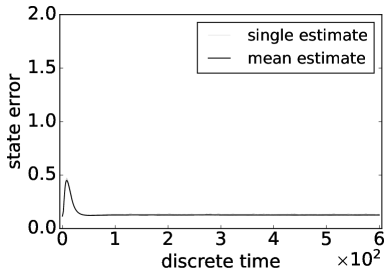
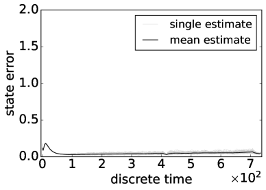
Figure 12: State errors of an SEIRS epidemic model for three contact networks in Table 2 using Algorithms 12 and 2^∗ for 100 independent runs in which the disease does not die out in 600 time steps for Facebook and Gowalla, and 733 time steps for AS-733. The first row is for Facebook, the second row is for Gowalla, and the third row is for AS-733. The left column uses the parameters $\beta=0.2,\sigma=1/3,\gamma=1/14,\rho=1/180,\lambda_{FP}=0.1,\lambda_{FN}=0.1$; the right column uses the parameters $\beta=0.27,\sigma=1/2,\gamma=1/7,\rho=1/90,\lambda_{FP}=0.1,\lambda_{FN}=0.3$. Light gray: state error from individual runs. Dark solid: mean state error averaged over 100 independent runs.

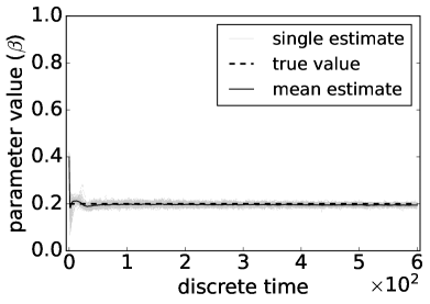
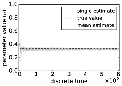
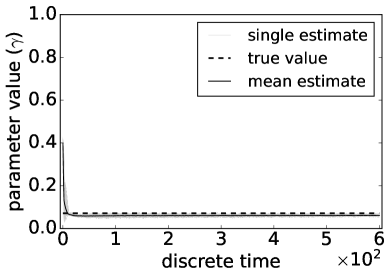
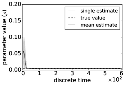
Figure 13: Parameter estimates of an SEIRS epidemic model for the Facebook contact network using Algorithms 12 and 2^∗ for 100 independent runs in which the disease does not die out in 600 time steps. The parameters are $\beta=0.2,\sigma=1/3,\gamma=1/14,\rho=1/180,\lambda_{FP}=0.1,\lambda_{FN}=0.1$. Light gray: parameter estimate from individual runs. Dark solid: mean parameter estimate averaged over 100 independent runs.

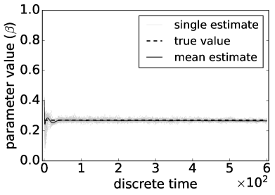
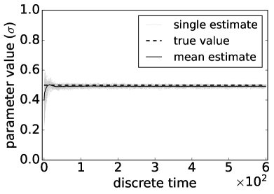
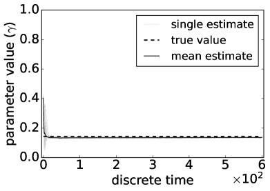
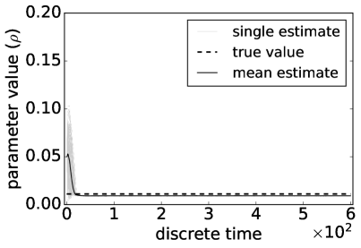
Figure 14: Parameter estimates of an SEIRS epidemic model for the Gowalla contact network using Algorithms 12 and 2^∗ for 100 independent runs in which the disease does not die out in 600 time steps. The parameters are $\beta=0.27,\sigma=1/2,\gamma=1/7,\rho=1/90,\lambda_{FP}=0.1,\lambda_{FN}=0.3$. Light gray: parameter estimate from individual runs. Dark solid: mean parameter estimate averaged over 100 independent runs.

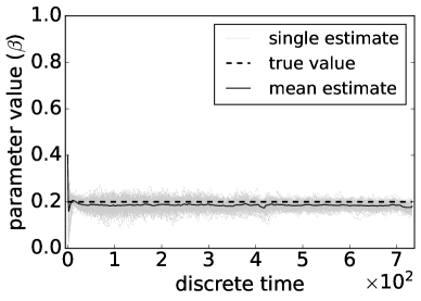
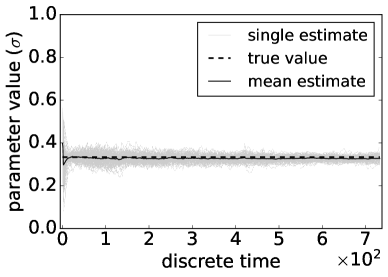
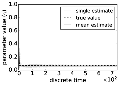
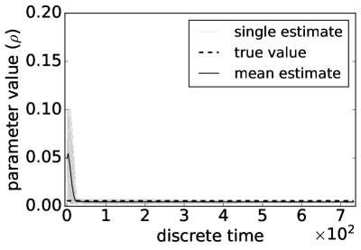
Figure 15: Parameter estimates of an SEIRS epidemic model for the AS-733 contact network using Algorithms 12 and 2^∗ for 100 independent runs in which the disease does not die out in 733 time steps. The parameters are $\beta=0.2,\sigma=1/3,\gamma=1/14,\rho=1/180,\lambda_{FP}=0.1,\lambda_{FN}=0.1$. Light gray: parameter estimate from individual runs. Dark solid: mean parameter estimate averaged over 100 independent runs.

Figure 12 shows the results of tracking states, and Figures 13, 14, and 15 the results of estimating parameters using factored conditional variational filtering (Algorithms 12 and 2^∗) for the Facebook, Gowalla, and AS-733 contact networks. The (hyper-)parameter values for the simulation transition model and filter transition update are $K=3$, $\kappa_{1}=0.2$, $\kappa_{2}=0.1$, and $M_{k}=10$, for $k=1,\ldots,L$. The parameter value for the simulation and filter observation models is $m=5$. The probability of a node being observed at a time step is $\alpha=0.7$. The number of parameter particles is $N=300$.

Here are some remarks about the comparison of the respective models used for Algorithms 9 and 12. The model for Algorithm 9 is primarily meant for the situation where a node is an individual; for Algorithm 12 a node is a subpopulation. We believe the concept of a subpopulation contact network has greater applicability than a simple contact network for which a node is an individual. The problem for the latter model is that it is generally difficult to know all the connections (that is, edges on the network) between individuals. For a subpopulation contact network, nodes can be communities of some kind and edges can represent (usually) fixed physical connections between them, such as transportation systems. Thus a subpopulation contact network can scale much better than a simple contact network.

For Algorithm 9, the Dirichlet observation model used is natural since it provides a noisy observation of the categorical distribution labelling a node. For Algorithm 12, since a node represents a subpopulation, a number of test results are likely to be returned. For this, the multinomial observation model is natural. Furthermore, as can be seen from the preceding analyses, the multinomial observation model leads to a much simpler algorithm because the Dirichlet distribution is the conjugate prior of the multinomial distribution. In fact, Algorithm 12 for the model of this section is much more efficient than Algorithm 9 for the model of Section LABEL:sec:FactoredVariationalFilter.

6 Related Work

Undoubtedly the best-known exact filter is the Kalman filter. Kalman filters produce closed-form estimates of the state posterior if both the transition and observation models are linear Gaussian. However, maintaining the closed-form covariance matrix for high dimensional states can be computationally expensive. This issue can be alleviated using the ensemble Kalman filters (EnKF) Evensen (1994, 2009), which resort to a sample covariance matrix estimated by a set of ensemble members (i.e., samples of states) maintained by the algorithm. Ensemble Kalman filters are widely adopted in atmospheric modelling Houtekamer and Mitchell (1998), ocean modelling Echevin et al. (2000); Park and Kaneko (2000), and estimating dynamics of infectious diseases Yang et al. (2014); Li et al. (2020).

Many modifications of the Kalman filter exist to deal with non-linear systems. The Extended Kalman Filter (EKF) approximates a solution by linearizing the system about the current mean and variance estimate so that the traditional linear Kalman Filter may be applied. When the system is highly non-linear however, the EKF can quickly diverge due to the covariance being propogated through a first-order linearization of the underlying non-linear system Wan and Van Der Merwe (2000). The Unscented Kalman Filter (UKF) addresses some of the EKF’s limitations by utilising an unscented transformation to pick a minimal set of sample points around the mean and covariance. The expected performance of the UKF was analytically shown to be superior to the EKF and directly comparable to a second-order Kalman Filter Julier and Uhlmann (1997).

If the transition and observation models are not linear Gaussian, one could resort to sampling-based methods such as particle filters, also known as sequential Monte Carlo methods Handschin and Mayne (1969); Akashi and Kumamoto (1977). When dealing with high-dimensional state variables, sampling could be inefficient which is a major drawback of particle filters. However, if there is structure in state variables that make the conditional posterior distribution of a subset of variables analytically tractable, employing the Rao-Blackwellization technique could reduce the dimension for sampling and therefore more efficient filtering could be achieved Doucet et al. (2000). There is also literature on using proposal distributions other than the transition model to address degeneracy issues in particle filtering Snyder et al. (2015); Naesseth et al. (2018). These techniques don’t scale to very high dimensions, but they do make particle filtering practical for dimensions up to 100 or so.

If the posterior distribution is expected to be closely approximated by an exponential family distribution, assumed density filtering methods can be considered. Assumed density filtering has been proposed independently in the statistics, artificial intelligence, and control literature and also goes by the names ‘moment matching’, and ‘online Bayesian learning’ Minka (2001a). Assumed density filtering proceeds in two general steps to approximate the posterior: the previous approximate posterior distribution is updated before being projected back into the chosen parametric family of distributions. The variational approach to filtering presented in Algorithm 3 bears close similarity to the idea of assumed density filtering.

Boyen and Koller (1998, 1999) introduced the idea of factoring, which exploited the structure of a large dynamic Bayesian network (DBN) for efficient approximate inference. The basic idea was to partition the dimension space to obtain tractable approximations of distributions on high-dimensional state spaces. Later, Ng et al. (2002) combined factoring with particle filtering to obtain a version of factored particle filters that is similar to the approach in Section 4. The main difference between factored particle filters as presented here and the version of Ng et al. (2002) is that here the particle family for the entire state space is maintained only in an implicit form; if the state distribution is needed, for example, to compute an integral, particles for the (entire) state are sampled from the implicit form. Later work along these lines includes that of Das et al. (2005). The approach here is also similar to that of Djurić and Bugallo (2013), and Djurić et al. (2007), which use the terminology multiple particle filter.

In parallel with the papers above in the artificial intelligence literature, factored particle filters were also studied in the data assimilation literature but using the term local particle filter. See the discussion on the origins of localization by van Leeuwen (2009). A particularly relevant is the paper of Rebeschini and Van Handel (2015) in which a local particle filter, called a block particle filter, is presented that is similar, but not identical, to the factored particle filter in Subsection 2.4. (A block is the same as a cluster.) This paper also contains a theorem that gives an approximation error bound for the block particle filter that could be adapted to the factored particle filter here. Poterjoy et al. (2019) provide a recent account of the use of local particle filters for data assimilation in large-scale geophysical applications, especially numerical weather prediction.

Coverage of relevant literature on parameter estimation using particle methods in state-space models can be found in the work of Kantas et al. (2015), Carvalho et al. (2010), and Andrieu et al. (2004). The origins of the nested particle filtering algorithm were discussed by Crisan and Miguez (2018). An early paper on conditional particle filters in the artificial intelligence literature is that of Montemerlo et al. (2002). The problem considered is that of simultaneously estimating the pose of a mobile robot and the positions of nearby people in a previously mapped environment. The algorithm proposed to solve the problem is a conditional particle filter that in effect treats the pose of the robot as the parameter space and the position of nearby people as the state space. A related approach is to augment the state with the parameter and compute joint posterior distributions over the state space and parameter. The EKF-SLAM filter utilizes such an approach Durrant-Whyte and Bailey (2006). Conversely, if one considers the state as originally comprising of the parameter, conditional particle filtering can be viewed as hierarchically decomposing the state into two components. This is the approach taken by Doucet and Johansen (2011). There are also other meanings of the term conditional particle filter in the literature. For example, for Svensson et al. (2015), the conditioning is with respect to a state space trajectory. A variational approach to the problem of state and parameter estimation has also been considered by Ye et al. (2015).

Whilst a wide array of exact and approximate approaches for conditional filtering and factored filtering have been explored in the literature, the combination of the two has been relatively unexplored. Kantas et al. (2006) proposed a recursive maximum-likelihood algorithm to tackle the problem of sensor registration and localisation. Each sensor is represented as a node in a graph and maintains its own coordinate system with a matrix of parameters denoting the offset of a given node in another node’s coordinate system. The parameters are estimated via gradient ascent on the log-likelihood function and each node maintains its own state filter. A crucial difference to our approach is that arbitrary clustering is only allowed via message passing in the observation update whilst a node’s transition update depends only upon its previous state, independent of neighbours. In this manner, our approach is strictly more general.

7 Conclusion

In this paper, we presented a framework for investigating the space of filtering algorithms. In particular, we presented the factored conditional filter, a filtering algorithm having three basic versions, for simultaneously tracking states and estimating parameters in high-dimensional state spaces. The conditional nature of the algorithm is used to estimate parameters and the factored nature is used to decompose the state space into low-dimensional subspaces in such a way that filtering on these subspaces gives distributions whose product is a good approximation to the distribution on the entire state space. We provided experimental results on tracking epidemics and estimating parameters in large contact networks that show the effectiveness of our approach.

There are several directions for future work. First, the three variations of the factored conditional particle filter we have presented are essentially the simplest possible algorithms that are both factored and conditional. It is likely that there are numerous improvements and optimizations that could be made to them. Typical such elaborations for a local particle filter intended for applications in the field of geophysics and similar in nature to the factored particle filter here are given by Poterjoy et al. (2019). While that algorithm is specialized to numerical weather prediction, it seems likely that many of the improvements and optimizations of Poterjoy et al. (2019) will also apply to the algorithm here.

Second, the factored conditional particle filter needs further theoretical foundations beyond that of Lloyd (2022). Crisan and Miguez (2017, 2018) give convergence theorems for the nested particle filter that is similar to the conditional particle filter presented here. Also Rebeschini (2014), and Rebeschini and Van Handel (2015) give an error approximation bound for their local particle filter, which is similar to the factored particle filter here. For our factored conditional particle filter, what is needed are convergence/error bound results that combine the results of Crisan and Miguez (2017, 2018), Rebeschini (2014), and Rebeschini and Van Handel (2015). Bounds on the approximations introduced by variational filters also needs investigation.

Third, for a particular application, the optimal partition for the factored particle filter lies somewhere between the finest and the coarsest partitions. It would be useful to develop criteria for choosing the appropriate partition. The partition cannot be finer than the observations allow, but there is scope for combining the smallest clusters allowed by the observations into larger clusters thus producing a coarser partition that may reduce the approximation error. On the other hand, a partition that is too coarse may lead to degeneracy problems.

Fourth, the experiments presented here are concerned only with the special case of state distributions (under the Markov assumption) and do not exploit the full generality of the empirical belief framework. It would be interesting to explore, for example, applications of a cognitive nature such as acquiring beliefs about the beliefs of other agents or applications where (a suitable summarization of) the history argument in the transition and/or observation model was needed.

Fifth, the variational versions of the algorithms could be developed more deeply. For example, it would be interesting to study a version of Algorithm 3 that employed variational inference, expectation propagation, or similar in the variational step and compare the results with those obtained by Algorithm 9 for which factorization is handled outside the variational step. For this, the ideas of Minka (2005) are likely to be useful. More generally, there is promise in developing variational filters instead of the more usual particle filters for appropriate applications.

Finally, the ultimate aim is for the filtering algorithms of this paper to be employed in agents of the kind described at the beginning of the Introduction. Thus the agents’ actions, selected using their empirical beliefs acquired by the filtering algorithms of this paper, perform useful functions in applications of practical importance.

Appendix A. A Discrete-Time Stochastic Lorenz System

The application here is that of a stochastic discrete-time Lorenz system studied in detail by Chorin and Krause (2004), and Crisan and Miguez (2018). This involves tracking the three-dimensional state and estimating the parameters of the Lorenz system, as illustrated in Figure 16(a). We perform the same experiments as those performed by Crisan and Miguez (2018) so that the results there can be compared with the results given here. For this application, both the filter for parameters and the conditional filter for states are particle filters, that is, the filter for parameters employs Algorithm 2^∗∗ and the conditional filter for states employs Algorithm 5.

Transition and Observation Models

The state of the Lorenz system at time $n$ is represented by a three-dimensional random vector $y_{n}=(y_{n,1},\,y_{n,2},\,y_{n,3})$, which are governed by the initial states $y_{\ast}=(-5.91652,-5.52332,\,24.5723)$ and the following stochastic transition model

$$y_{n+1,1}\sim\mathcal{N}(y_{n,1}-\Delta t\,\theta_{1}(y_{n,1}-y_{n,2}),\,\Delta t),$$ (43)

$$y_{n+1,2}\sim\mathcal{N}(y_{n,2}+\Delta t\,(\theta_{2}y_{n,1}-y_{n,2}-y_{n,1}y_{n,3}),\,\Delta t),$$

$$y_{n+1,3}\sim\mathcal{N}(y_{n,3}+\Delta t\,(y_{n,1}y_{n,2}-\theta_{3}y_{n,3}),\,\Delta t),\text{ for all $n\in\mathbb{N}_{0}$},$$

where $\mathcal{N}(\mu,\sigma^{2})$ denotes the Gaussian distribution with mean $\mu$ and variance $\sigma^{2}$. The step size $\Delta t=0.001$ and the true values of parameters $\theta_{1}=10,\ \theta_{2}=28,\ \theta_{3}=8/3$.

Further, the state is partially observed with Gaussian noise every $40$ steps,

$$o_{n,1}\sim\mathcal{N}(\theta_{4}y_{n,1},\,0.1),$$ (44)

$$o_{n,3}\sim\mathcal{N}(\theta_{4}y_{n,3},\,0.1),\text{ for all $n\in\{40t:t\in\mathbb{N}\}$},$$

where $o_{n}=(o_{n,1},o_{n,3})$ is the observation at time $n$, and the scale parameter in the observation model $\theta_{4}=4/5$.

Empirical Evaluation

Experimental setup

We adopt a similar setup as that presented by Crisan and Miguez (2018), and employ Algorithms 2^∗∗ and 5 to track states and estimate parameters at the same time. First, the initial conditional particle family $((x_{0}^{(i)},(y_{0}^{(i,j)})_{j=1}^{M}))_{i=1}^{N}$ are produced by

$$x_{0,1}^{(i)}\sim\mathcal{U}(5,20),\ \ \ x_{0,2}^{(i)}\sim\mathcal{U}(18,50),\ \ \ x_{0,3}^{(i)}\sim\mathcal{U}(1,8),\ \ \ x_{0,4}^{(i)}\sim\mathcal{U}(0.5,3),$$ (45)

$$y_{0}^{(i,j)}\sim\mathcal{N}(y_{\ast},10I_{3}),\text{ for }i=1,\dots,N\text{ and }j=1,\dots,M,$$

where $\mathcal{U}(a,b)$ is the uniform distribution over interval $(a,b)$, $I_{3}$ is the identity matrix of size 3, and $N=M=300$ specifying the number of parameter particles and conditional particles.

Next, as a baseline, we use a Gaussian jittering kernel with a covariance matrix that does not change over time, i.e.,

$$\Sigma_{n}=N^{-\frac{3}{2}}\,\text{diag}(60,60,10,1),\text{ for all }n\in\mathbb{N},$$ (46)

where $\,\text{diag}(60,60,10,1)$ is a diagonal matrix with diagonal entries $(60,60,10,1)$.

Alternatively, one may want to adapt the jittering over time, for example, by encouraging exploration at the beginning of the stochastic process, while gradually putting more effort on exploitation as the process evolves. A simple example of such adaptive jittering is using a Gaussian kernel with the following covariance matrix,

$$\Sigma_{n}=\max(ar^{n},b)\,N^{-\frac{3}{2}}\,\text{diag}(60,60,10,1),\text{ for all }n\in\mathbb{N},$$ (47)

where $a>b>0$ and $r\in(0,1)$. We empirically evaluate both jittering techniques, and $a=25,b=0.01,r=0.996$ are employed for the adaptive jittering in our experiment.

Evaluation

We evaluate the performance of state tracking by the Euclidean distance between the true state and the estimated state,

$$\left\|\widetilde{y}_{n}-\widehat{y}_{n}\right\|_{2},\text{ for all }n\in\mathbb{N},$$ (48)

where $\widetilde{y}_{n}$ is the true state at step $n$ in the underlying simulation of the Lorenz system, and the estimated state $\widehat{y}_{n,l}=\frac{1}{NM}\sum_{i=1}^{N}\sum_{j=1}^{M}y^{(i,j)}_{n,l},\text{ for }l=1,2,3$.

Following Crisan and Miguez (2018), we evaluate the estimated parameters of the Lorenz system at step $n$ using the normalized error

$$|(\widehat{x}_{n,k}-\theta_{k})/\theta_{k}|,\text{ for all }n\in\mathbb{N}\text{ and }k=1,2,3,4,$$ (49)

where the estimate $\widehat{x}_{n,k}=\frac{1}{N}\sum_{i=1}^{N}x^{(i)}_{n,k}$, for $k=1,2,3,4$, and the true parameter values $\theta=(10,28,8/3,4/5)$. (Note that this is a different definition of parameter error to that defined and used elsewhere in this paper. Here the same definition as Crisan and Miguez (2018) is used so a direct comparison can be made between the results in that paper and those given here.)

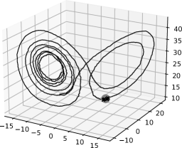
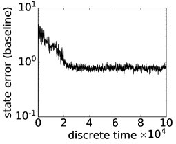
(a)	(b)	(c)

Figure 16: Tracking states of the stochastic Lorenz system. (a): An illustration of the stochastic Lorenz system. Dark curve: trajectory of the Lorenz system; Gray ball: the position of the Lorenz system at a particular time; Dark cross: particles tracking the state of the Lorenz system. (b): Mean distances corresponding to the results in Figure 17. (c): Mean distances corresponding to the results in Figure 18.

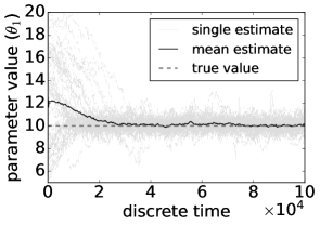
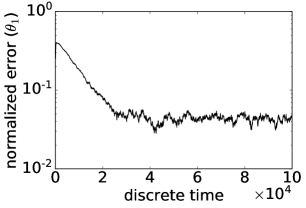
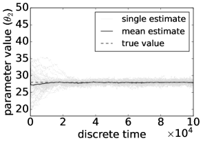
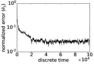
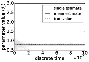
Figure 17: Estimating each of the four parameters of a stochastic Lorenz system with Algorithms 2^∗∗ and 5 in 50 independent runs. We employ a Gaussian jittering kernel with the static covariance matrix (Eq. 46) in Algorithm 2^∗∗. Each run of the algorithms corresponds to a simulation of the system for $10^{5}$ discrete time steps according to the transition model (Eq. 43), and system states are observed every 40 time steps according to the observation model (Eq. 44). The number of particles employed are $M=N=300$ and true parameter values are $\theta=(10,\,28,\,8/3,\,4/5)$. Left column: each of the four parameters estimated from individual runs (light gray), mean estimation averaged over 50 independent runs (dark solid) and true parameter values (dark dash). Right column: the normalized error of each parameter (Eq. 49) averaged over the same 50 independent runs.

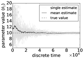
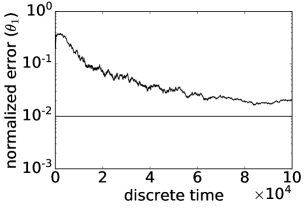
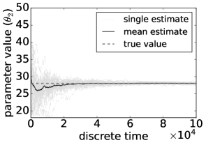
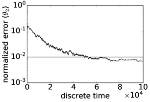
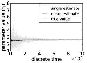
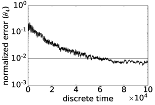
Figure 18: Estimating each of the four parameters of a stochastic Lorenz system with Algorithms 2^∗∗ and 5 in 50 independent runs. The experimental setup is the same as that of Figure 17, except that an adaptive Gaussian jittering kernel with covariance matrix Eq. (47) is employed in Algorithm 2^∗∗. Left column: each of the four parameters estimated from individual runs (light gray), mean estimation averaged over 50 independent runs (dark solid) and true parameter values (dark dash). Right column: the normalized error of each parameter (Eq. 49) averaged over the same 50 independent runs; noting that the range of y-axis is $(10^{-3},1)$ and a straight line representing $10^{-2}$ is shown to facilitate the comparison with results in the right column of Figure 17.

Results and discussion

Figures 16(b) and 16(c) shows the Euclidean distances over time between the true states from the underlying simulation and the states tracked by the conditional particle filter. The distances are averaged over 50 independent runs. We can see the mean distances in both Figure 16(b) and Figure 16(c) are less than $1$ after $20,000$ steps, which is reasonably accurate considering the average distance the system moved in a single transition is approximately $3.65$, and the ranges of states in the three-dimension are respectively $(-19.06,18.92)$, $(-25.86,26.01)$ and $(2.29,46.98)$ in all the 50 simulations.

Figure 17 shows the results of estimating parameters for the discrete-time stochastic Lorenz system using Algorithms 2^∗∗ and 5 with the baseline jittering, i.e., the covariance matrix of the Gaussian jittering kernel is Eq. (46). We performed 50 independent runs of the experiment to evaluate the expected behavior. The left column of Figure 17 details the estimation of the four parameters over time, including estimation from each individual run of the experiment (light gray), the mean estimation over all independent runs (solid dark) and the true parameter values (dashed dark). The right column of Figure 17 shows the normalized error (Eq. 49) of each parameter averaged over the 50 independent runs. These results are highly similar to those presented by Crisan and Miguez (2018). (See Figure 1 in that paper.) However, with the use of the Gaussian jittering kernel with covariance matrix Eq. (47), which is a simple example of adaptive jittering, we achieved more accurate estimations of the parameters, as shown in Figure 18.

The experimental results presented in this section correspond closely to the results presented by Crisan and Miguez (2018). In fact, the combination of Algorithm 2^∗∗ and Algorithm 5 is similar to the nested particle filter proposed by Crisan and Miguez (2017, 2018), as explained in Section 2.3. However, the discovery of the conditional particle filter came from a different motivation: how to acquire (by filtering) empirical beliefs whose codomains are the space of probability distributions on a structured space, such as a space of sets, multisets, lists, or function spaces. The presence of these structured spaces suggested deconstructing an empirical belief into two or more levels of ‘simpler’ empirical beliefs which in turn led to the paired Algorithms 2^∗∗ and 5. The formulation of the conditional particle filter has a clean separation between the parameter and state levels. Furthermore, it can be used for applications beyond the estimation of parameters. The nested particle filter mixes the two levels into a single algorithm, thus arguably missing some conceptual simplicity.

Appendix B. A Conditional Particle Filter for Epidemic Processes

As we have shown in Sections 3, 4 and 5, epidemic processes are a suitable application domain for exploiting the factorization assumption for state distributions. In this appendix, we study the effect of not exploiting this factorization assumption. Without this assumption, the problem becomes one of tracking a state distribution on a product space with a particle filter, where the particle family giving the state distribution is a subset of the product space. As expected, we show such an approach only works for low-dimensional product spaces.

Next the effectiveness of the algorithms in Section 2 for filtering on graphs is empirically demonstrated. Consider an epidemic process spreading on a contact network, as described in Section 3. We employ conditional filtering to track states and estimate the parameters of epidemics on small contact networks. For this application, both the filter for parameters and the conditional filter for states are particle filters, i.e., the filter for parameters employs Algorithm 2^∗∗ and the conditional filter for states employs Algorithm 5.

We simulate an infectious disease on two small graphs, which are social networks employed as contact networks among individuals. The first graph is a social network of $34$ club members Zachary (1977), and the other graph is a social network of $62$ dolphins Lusseau et al. (2003). Let $C=\{\mathsf{S},\mathsf{I}\}$. We assume the disease spreads over the contact network following the transitions of an SIS epidemic model (Eq. (60)) below with transmission probability $\beta=0.2$ and average infectious period $\gamma^{-1}=10$ days, and no immunity gained upon recovery.

For all $n\in\mathbb{N}$ and $k=1,\ldots,L$, define

$$\breve{\tau}_{n}^{(k)}:C^{L}\rightarrow\mathcal{D}(C)$$

by

$$\breve{\tau}_{n}^{(k)}(s)(c)=\begin{cases}1-(1-\beta)^{d_{k}(s)}&\text{if $s_{k}=\mathsf{S}$ and $c=\mathsf{I}$}\\ (1-\beta)^{d_{k}(s)}&\text{\text{if $s_{k}=\mathsf{S}$ and $c=\mathsf{S}$}}\\ \gamma&\text{if $s_{k}=\mathsf{I}$ and $c=\mathsf{S}$}\\ 1-\gamma&\text{\text{if $s_{k}=\mathsf{I}$ and $c=\mathsf{I}$}},\end{cases}$$ (60)

where $s\in C^{L}$, $c\in C$, and $d_{k}(s)$ is the number of infected neighbours of node $k$.

The observation model is given by Eq. (61). For all $n\in\mathbb{N}$ and $k=1,\ldots,L$,

$$\breve{\xi}_{n}^{(k)}:C\to\mathcal{D}(O)$$

is defined by

$$\breve{\xi}_{n}^{(k)}(\mathsf{S})(\texttt{+})=\alpha_{\mathsf{S}}\lambda_{FP}, \breve{\xi}_{n}^{(k)}(\mathsf{I})(\texttt{+})=\alpha_{\mathsf{I}}(1-\lambda_{FN}),$$ (61)

$$\breve{\xi}_{n}^{(k)}(\mathsf{S})(\texttt{-})=\alpha_{\mathsf{S}}(1-\lambda_{FP}), \breve{\xi}_{n}^{(k)}(\mathsf{I})(\texttt{-})=\alpha_{\mathsf{I}}\lambda_{FN},$$

$$\breve{\xi}_{n}^{(k)}(\mathsf{S})(\texttt{?})=1-\alpha_{\mathsf{S}}, \breve{\xi}_{n}^{(k)}(\mathsf{I})(\texttt{?})=1-\alpha_{\mathsf{I}}.$$

Here, $\alpha_{\mathsf{S}}$ and $\alpha_{\mathsf{I}}$ are the probability that a susceptible and infected individual, respectively, is tested. Also, $\lambda_{FP}$ is the false positive rate of the testing method and $\lambda_{FN}$ is the false negative rate. We assume $\alpha_{S}=0.1$ and $\alpha_{I}=0.9$, which means that an infected individual is highly likely to be tested due to, for example, symptoms, and approximately $1$ in $10$ healthy (susceptible) individuals in the population will be tested as a result of large-scale random testing. And we further assume the testing method employed has a $10\%$ false positive rate and a $10\%$ false negative rate, i.e., $\lambda_{FP}=\lambda_{FN}=0.1$.

We start a simulation by choosing an individual, that is, a node, uniformly at random from the set of all nodes in the graph and make it infected (i.e., the patient zero); all other nodes in the contact network are susceptible; we then evolve the transition model (Eq. (60)) for 600 time steps and generate observations according to the observation model (Eq. (61)) in each time step.

Experimental setup

A parameter particle filter with 300 particles is employed, so that $N=300$. The parameter particle family is initialized by sampling from uniform distributions as follows:

$$x_{n_{\ast},1}^{(i)}\sim\mathcal{U}(0,0.8),\ \ \ x_{n_{\ast},2}^{(i)}\sim\mathcal{U}(0,0.8),$$

where $i\in\{1,\dots,N\}$ and $n_{\ast}\in\mathbb{N}$ is defined below.

The initial state distribution of an epidemic is usually unknown and we have to estimate it, for example, using information of the reported positive cases. Let $n_{\ast}$ be the time step when the number of reported positive cases from testing surpasses, for the first time, a predefined threshold, and suppose that most individuals in the population are susceptible at time $n_{\ast}$. The initial state distribution is then estimated by performing an observation update using the observation at time $n_{\ast}$. In particular, let $(p_{k},1-p_{k})$ denote the tuple of (estimated) probabilities for the compartments, in the order $\mathsf{S}$, $\mathsf{I}$, for node $k$ at time $n_{\ast}$. The state particle families are initialized by sampling from categorical distributions as follows:

$$y_{n_{\ast},k}^{(i,j)}\sim Cat(p_{k},1-p_{k})$$

for $k=1,\dots,L$, $i=1,\dots,N$ and $j=1,\dots,M$. Here $Cat(p_{k},1-p_{k})$ is a categorical distribution for which the parameters are $p_{k}$ and $1-p_{k}$.

We determine the number of state particles $M$ using a formula suggested by Snyder et al. (2008),

$$M=10^{0.05d+0.78},$$ (62)

where $d$ is the state dimension. This formula was developed empirically from a simple application for a lower bound on the number of particles that is needed for filtering to perform reasonably well. Thus, for $d=34,M\approx 300$ and, for $d=62,M\approx 7600$. While the formula given by Eq. (62) is at most an approximate lower bound for a rather simpler problem than an SIS epidemic, it seemed worthwhile to try these values for the state particle family sizes for the graphs of 34 and 62 nodes in the experiments.

We also leverage an adaptive Gaussian jittering kernel in Algorithm 2^∗∗ with covariance matrix

$$\Sigma_{n}=\max(ar^{n},b)\mathbf{I}_{2},\ n\in\mathbb{N},$$ (63)

where $a=10^{-4},b=9\times 10^{-6},r=0.996$, and $\mathbf{I}_{2}$ is the identity matrix of size 2.

Evaluation

The performance of the filter in tracking states is now investigated. As explained in Section 3.5, it is sufficient to define a suitable metric $\rho$ on $C^{L}$. Let $\kappa:C\times C\rightarrow\mathbb{R}$ be the discrete metric on $C$ and $\rho:C^{L}\times C^{L}\rightarrow\mathbb{R}$ the metric on $C^{L}$ defined by

$$\rho(y,z)=\frac{1}{L}\sum_{k=1}^{L}\kappa(y_{k},z_{k}),$$

for all $y,z\in C^{L}$. Let $\widetilde{y}_{n}\in C^{L}$ be the ground truth state at time $n$. Suppose that

$$\savestack{\tmpbox}{\stretchto{\scaleto{\scalerel*[width("(\nu_{n}\odot\mu_{n})(h_{n})")]{\kern-0.6pt\bigwedge\kern-0.6pt}{\rule[-614.295pt]{4.30554pt}{614.295pt}}}{}}{0.5ex}}\stackon[1pt]{(\nu_{n}\odot\mu_{n})(h_{n})}{\tmpbox}=\frac{1}{NM}\sum_{i=1}^{N}\sum_{j=1}^{M}\delta_{y^{(i,j)}_{n}}$$

is the filter’s estimate of the state distribution at time $n$. Then

Thus

$$\mathit{Err}((\savestack{\tmpbox}{\stretchto{\scaleto{\scalerel*[width("\nu_{n}\odot\mu_{n})(h_{n})")]{\kern-0.6pt\bigwedge\kern-0.6pt}{\rule[-614.295pt]{4.30554pt}{614.295pt}}}{}}{0.5ex}}\stackon[1pt]{\nu_{n}\odot\mu_{n})(h_{n})}{\tmpbox})=\frac{1}{NML}\sum_{i=1}^{N}\sum_{j=1}^{M}\sum_{k=1}^{L}\kappa(\widetilde{y}_{n,k},y_{n,k}^{(i,j)}).$$

For the parameters, the error is given by Eq. (16), so that

$$\mathit{Err}_{j}(\savestack{\tmpbox}{\stretchto{\scaleto{\scalerel*[width("\nu_{n}(h_{n})")]{\kern-0.6pt\bigwedge\kern-0.6pt}{\rule[-614.295pt]{4.30554pt}{614.295pt}}}{}}{0.5ex}}\stackon[1pt]{\nu_{n}(h_{n})}{\tmpbox})=\frac{1}{\widetilde{x}_{j}}\frac{1}{N}\sum_{i=1}^{N}|\widetilde{x}_{j}-x^{(i)}_{n,j}|,$$

for $j=1,2$. Here $\widetilde{x}_{1}=\beta$ and $\widetilde{x}_{2}=\gamma$.

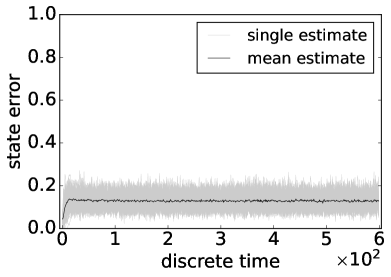
Figure 19: State errors of tracking SIS epidemics on small contact networks using the conditional particle filter (i.e., Algorithms 2^∗∗ and 5) in 100 independent runs in which the disease does not die out in 600 time steps. The true values of transmission probability $\beta=0.2$ and average recovery period $\gamma^{-1}=10$ days. Left: using a contact network with 34 nodes Zachary (1977), and the number of particles employed are $N=300,M=300$. Right: using a contact network with $62$ nodes Lusseau et al. (2003), and the number of particles employed are $N=300,M=7,600$. Light gray: state errors from individual runs. Dark solid: mean state error averaged over 100 independent runs.

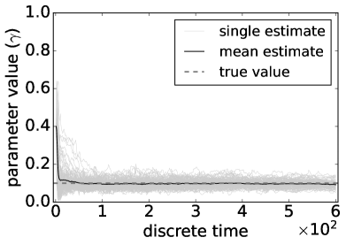
Figure 20: Estimating parameters of an SIS epidemic on a small contact network with 34 nodes Zachary (1977) using the conditional particle filter (i.e., Algorithms 2^∗∗ and 5) in 100 independent runs in which the disease does not die out in 600 time steps. The number of particles employed are $N=300,M=300$, and the true values of transmission probability $\beta=0.2$ and average recovery period $\gamma^{-1}=10$ days. Light gray: estimated value from individual runs. Dark solid: mean estimation averaged over 100 independent runs. Dark dash: true values of parameters.

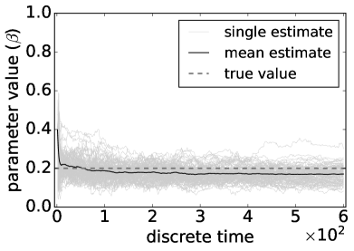
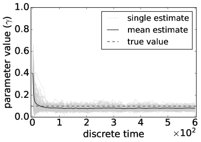
Figure 21: Estimating parameters of an SIS epidemic on a small contact network with $62$ nodes Lusseau et al. (2003) using the conditional particle filter (Algorithms 2^∗∗ and 5) in 100 independent runs in which the disease does not die out in 600 time steps. The number of particles employed are $N=300,M=7,600$, and the true values of transmission probability $\beta=0.2$ and average recovery period $\gamma^{-1}=10$ days. Light gray: estimated value from individual runs. Dark solid: mean estimation averaged over 100 independent runs. Dark dash: true values of parameters.

Results and discussion

Figure 19 shows the results of tracking states, and Figures 20 and 21 the results of estimating parameters using the conditional particle filter (Algorithms 5 and 2^∗∗) on the two small contact networks with 34 and 62 nodes.

We have seen the state particle family sizes suggested by Eq. (62) proved to be good lower bounds – filtering worked well enough with those sizes for both graphs. Further, we note that the accuracy of state tracking and parameter estimation are remarkably similar between the two cases, the reason might be the difference in dimension is counterbalanced by the number of state particles. We remark that with smaller state particle families, the experimental results were not as good, and unsurprisingly, with bigger state particle families, the experimental results were better, for each graph.

On the other hand, according to Eq. (62), for $d=80$, $M$ is approximately $60,000$, but for $d=100$, $M$ will exceed $600,000$, which is not all that feasible. This suggests that for contact networks much larger than those considered in this appendix, it is necessary to exploit the structural properties of epidemics, such as factorization. Our experiments with larger contact networks, not using factorization, produced poor results and thus confirmed this view.

References

- Akashi and Kumamoto (1977) Hajime Akashi and Hiromitsu Kumamoto. Random sampling approach to state estimation in switching environments. Automatica, 13(4):429–434, 1977.
- Anderson (2013) Roy M Anderson. The population dynamics of infectious diseases: theory and applications. Springer, 2013.
- Andrieu et al. (2004) Christophe Andrieu, Arnaud Doucet, Sumeetpal S Singh, and Vladislav B Tadic. Particle methods for change detection, system identification, and control. Proceedings of the IEEE, 92(3):423–438, 2004.
- Bengtsson et al. (2008) T. Bengtsson, P. Bickel, and B. Li. Curse-of-dimensionality revisited: Collapse of the particle filter in very large scale systems. IMS Collections. Probability and Statistics: Essays in Honor of David A. Freedman, 2:316–334, 2008.
- Bickel et al. (2008) P. Bickel, B. Li, and T. Bengtsson. Sharp failure rates for the bootstrap particle filter in high dimensions. IMS Collections. Pushing the Limits of Contemporary Statistics: Contributions in Honor of Jayanta K. Ghosh, 3:318–329, 2008.
- Bishop (2006) C.M. Bishop. Pattern Recognition and Machine Learning. Springer, 2006.
- Bjørnstad et al. (2020) O. Bjørnstad, K. Shea, M. Krzywinski, and N. Altman. The SEIRS model for infectious disease dynamics. Nature Methods, 17:557–558, 2020.
- Blei et al. (2017) D. Blei, A. Kucukelbir, and J. McAuliffe. Variational inference: A review for statisticians. Journal of the American Statistical Association, 112(518):859–877, 2017.
- Blum et al. (2020) A. Blum, J. Hopcroft, and R. Kannan. Foundations of Data Science. Cambridge University Press, 2020.
- Boyen and Koller (1998) Xavier Boyen and Daphne Koller. Tractable inference for complex stochastic processes. In Proceedings of the Fourteenth Conference on Uncertainty in Artificial Intelligence, pages 33–42, 1998.
- Boyen and Koller (1999) Xavier Boyen and Daphne Koller. Exploiting the architecture of dynamic systems. In Proceedings of the Sixteenth National Conference on Artificial Intelligence (AAAI-99), pages 313–320, 1999.
- Brauer and Castillo-Chávez (2012) Fred Brauer and Carlos Castillo-Chávez. Mathematical Models in Population Biology and Epidemiology. Springer, 2012.
- Camacho et al. (2011) Anton Camacho, Sébastien Ballesteros, Andrea L Graham, Fabrice Carrat, Oliver Ratmann, and Bernard Cazelles. Explaining rapid reinfections in multiple-wave influenza outbreaks: Tristan da Cunha 1971 epidemic as a case study. Proceedings of the Royal Society B: Biological Sciences, 278(1725):3635–3643, 2011.
- Carvalho et al. (2010) Carlos M Carvalho, Michael S Johannes, Hedibert F Lopes, and Nicholas G Polson. Particle learning and smoothing. Statistical Science, 25(1):88–106, 2010.
- CDC (2019) CDC. Key Facts About Influenza. https://www.cdc.gov/flu/about/keyfacts.htm, 2019. retrieved May 2021.
- CDC (2020) CDC. Overview of Influenza Testing Methods. https://www.cdc.gov/flu/professionals/diagnosis/overview-testing-methods.htm, 2020. retrieved May 2021.
- Cho et al. (2011) Eunjoon Cho, Seth A Myers, and Jure Leskovec. Friendship and mobility: user movement in location-based social networks. In Proceedings of the 17th ACM SIGKDD international conference on Knowledge discovery and data mining, pages 1082–1090, 2011.
- Chopin et al. (2013) Nicolas Chopin, Pierre E. Jacob, and Omiros Papaspiliopoulos. SMC2: an efficient algorithm for sequential analysis of state space models. Journal of the Royal Statistical Society: Series B (Statistical Methodology), 75(3):397–426, 2013.
- Chorin and Krause (2004) Alexandre J Chorin and Paul Krause. Dimensional reduction for a Bayesian filter. Proceedings of the National Academy of Sciences, 101(42):15013–15017, 2004.
- Cohen and Burbelo (2020) Jeffrey I Cohen and Peter D Burbelo. Reinfection with SARS-CoV-2: Implications for Vaccines. Clinical Infectious Diseases, 0(0):1–6, 12 2020. doi: 10.1093/cid/ciaa1866. URL https://doi.org/10.1093/cid/ciaa1866.
- Crisan and Miguez (2017) Dan Crisan and Joaquin Miguez. Uniform convergence over time of a nested particle filtering scheme for recursive parameter estimation in state-space Markov models. Advances in Applied Probability, 49(4):1170–1200, 2017.
- Crisan and Miguez (2018) Dan Crisan and Joaquin Miguez. Nested particle filters for online parameter estimation in discrete-time state-space Markov models. Bernoulli, 24(4A):3039–3086, 2018.
- Das et al. (2005) Subrata Das, David Lawless, Brenda Ng, and Avi Pfeffer. Factored particle filtering for data fusion and situation assessment in urban environments. In Proceedings of the Seventh International Conference on Information Fusion, pages 955–962, 2005.
- Della Rossa et al. (2020) Fabio Della Rossa, Davide Salzano, Anna Di Meglio, Francesco De Lellis, Marco Coraggio, Carmela Calabrese, Agostino Guarino, Ricardo Cardona-Rivera, Pietro De Lellis, Davide Liuzza, et al. A network model of Italy shows that intermittent regional strategies can alleviate the COVID-19 epidemic. Nature Communications, 11(1):1–9, 2020.
- Dinnes et al. (2021) Jacqueline Dinnes, Jonathan J Deeks, Sarah Berhane, Melissa Taylor, Ada Adriano, Clare Davenport, Sabine Dittrich, Devy Emperador, Yemisi Takwoingi, Jane Cunningham, et al. Rapid, point-of-care antigen and molecular-based tests for diagnosis of SARS-CoV-2 infection. Cochrane Database of Systematic Reviews, 3, 2021.
- Djurić and Bugallo (2013) P. Djurić and M. Bugallo. Particle filtering for high-dimensional systems. In 5th IEEE International Workshop on Computational Advances in Multi-Sensor Adaptive Processing, CAMSAP 2013, pages 352––355, 2013.
- Djurić et al. (2007) P. Djurić, T. Lu, and M. Bugallo. Multiple particle filtering. In IEEE International Conference on Acoustics, Speech and Signal Processing, ICASSP 2007, pages 1181––1184, 2007.
- Doucet and Johansen (2011) A. Doucet and A.M. Johansen. Tutorial on particle filtering and smoothing: Fifteen years later. In D. Crisan and B. Rozovskii, editors, The Oxford Handbook of Nonlinear Filtering. Oxford University Press, 2011.
- Doucet et al. (2000) Arnaud Doucet, Nando de Freitas, Kevin Murphy, and Stuart Russell. Rao-Blackwellised particle filtering for dynamic Bayesian networks. In Proceedings of the Sixteenth conference on Uncertainty in Artificial Intelligence, pages 176–183, 2000.
- Durrant-Whyte and Bailey (2006) Hugh Durrant-Whyte and Tim Bailey. Simultaneous localization and mapping: part i. IEEE robotics & automation magazine, 13(2):99–110, 2006.
- Echevin et al. (2000) Vincent Echevin, Pierre De Mey, and Geir Evensen. Horizontal and vertical structure of the representer functions for sea surface measurements in a coastal circulation model. Journal of Physical Oceanography, 30(10):2627–2635, 2000.
- Evensen (1994) Geir Evensen. Sequential data assimilation with a nonlinear quasi-geostrophic model using Monte Carlo methods to forecast error statistics. Journal of Geophysical Research: Oceans, 99(C5):10143–10162, 1994.
- Evensen (2009) Geir Evensen. Data assimilation: the ensemble Kalman filter. Springer Science & Business Media, 2009.
- Gatto et al. (2020) Marino Gatto, Enrico Bertuzzo, Lorenzo Mari, Stefano Miccoli, Luca Carraro, Renato Casagrandi, and Andrea Rinaldo. Spread and dynamics of the COVID-19 epidemic in Italy: Effects of emergency containment measures. Proceedings of the National Academy of Sciences, 117(19):10484–10491, 2020.
- Gordon et al. (1993) Neil J Gordon, David J Salmond, and Adrian FM Smith. Novel approach to nonlinear/non-Gaussian Bayesian state estimation. IEE Proceedings F (Radar and Signal Processing), 140:107–113(6), 1993.
- Handschin and Mayne (1969) Johannes Edmund Handschin and David Q Mayne. Monte Carlo techniques to estimate the conditional expectation in multi-stage non-linear filtering. International Journal of Control, 9(5):547–559, 1969.
- Hethcote (2000) Herbert W Hethcote. The mathematics of infectious diseases. SIAM Review, 42(4):599–653, 2000.
- Houtekamer and Mitchell (1998) Peter L Houtekamer and Herschel L Mitchell. Data assimilation using an ensemble Kalman filter technique. Monthly Weather Review, 126(3):796–811, 1998.
- Jordan et al. (1999) M.I. Jordan, Z. Ghahramani, T.S. Jaakkola, and L.K Saul. An introduction to variational methods for graphical models. Machine Learning, 37:183–233, 1999.
- Julier and Uhlmann (1997) Simon J Julier and Jeffrey K Uhlmann. New extension of the kalman filter to nonlinear systems. In Signal processing, sensor fusion, and target recognition VI, volume 3068, pages 182–193. International Society for Optics and Photonics, 1997.
- Kantas et al. (2006) Nikolas Kantas, Sumeetpal S. Singh, and Arnaud Doucet. A distributed recursive maximum likelihood implementation for sensor registration. In 9th International Conference on Information Fusion, pages 1–8, 2006.
- Kantas et al. (2015) Nikolas Kantas, Arnaud Doucet, Sumeetpal S. Singh, Jan Maciejowski, and Nicolas Chopin. On Particle Methods for Parameter Estimation in State-Space Models. Statistical Science, 30(3):328 – 351, 2015.
- Kermack and McKendrick (1927) William Ogilvy Kermack and Anderson G McKendrick. A contribution to the mathematical theory of epidemics. Proceedings of the Royal Society of London, series A, 115(772):700–721, 1927.
- Klimt and Yang (2004) Bryan Klimt and Yiming Yang. The Enron corpus: A new dataset for email classification research. In European Conference on Machine Learning, pages 217–226, 2004.
- Leskovec et al. (2005) Jure Leskovec, Jon Kleinberg, and Christos Faloutsos. Graphs over time: densification laws, shrinking diameters and possible explanations. In Proceedings of the eleventh ACM SIGKDD International Conference on Knowledge Discovery in Data Mining, pages 177–187, 2005.
- Li et al. (2020) Ruiyun Li, Sen Pei, Bin Chen, Yimeng Song, Tao Zhang, Wan Yang, and Jeffrey Shaman. Substantial undocumented infection facilitates the rapid dissemination of novel coronavirus (SARS-CoV-2). Science, 368(6490):489–493, 2020.
- Lloyd (2022) J.W. Lloyd. Empirical Beliefs. Available at http://users.cecs.anu.edu.au/~jwl, 2022.
- Lumley et al. (2021) Sheila F Lumley, Denise O’Donnell, Nicole E Stoesser, Philippa C Matthews, Alison Howarth, Stephanie B Hatch, Brian D Marsden, Stuart Cox, Tim James, Fiona Warren, et al. Antibody status and incidence of SARS-CoV-2 infection in health care workers. New England Journal of Medicine, 384(6):533–540, 2021.
- Lusseau et al. (2003) David Lusseau, Karsten Schneider, Oliver J Boisseau, Patti Haase, Elisabeth Slooten, and Steve M Dawson. The bottlenose dolphin community of Doubtful Sound features a large proportion of long-lasting associations: Can geographic isolation explain this unique trait? Behavioral Ecology and Sociobiology, 54(4):396–405, 2003.
- Minka (2005) T. Minka. Divergence measures and message passing. Technical Report MSR-TR-2005-173, Microsoft Research Cambridge, 2005.
- Minka (2001a) T.P. Minka. A Family of Algorithms for Approximate Bayesian Inference. PhD thesis, MIT, 2001a.
- Minka (2001b) T.P. Minka. Expectation propagation for approximate Bayesian inference. In J. Breese and D. Koller, editors, Proceedings of the Seventeenth Conference on Uncertainty in Artificial Intelligence, pages 362–369. Morgan Kaufmann, 2001b.
- Mislove et al. (2007) Alan Mislove, Massimiliano Marcon, Krishna P Gummadi, Peter Druschel, and Bobby Bhattacharjee. Measurement and analysis of online social networks. In Proceedings of the 7th ACM SIGCOMM Conference on Internet Measurement, pages 29–42, 2007.
- Montemerlo et al. (2002) M. Montemerlo, S. Thrun, and W. Whittaker. Conditional particle filters for simultaneous mobile robot localization and people-tracking. In IEEE International Conference on Robotics and Automation, pages 695–701, 2002.
- Murphy (2012) K.P. Murphy. Machine Learning: A Probabilistic Perspective. MIT press, 2012.
- Naesseth et al. (2018) Christian A. Naesseth, Scott W. Linderman, Rajesh Ranganath, and David M. Blei. Variational sequential monte carlo. In Amos J. Storkey and Fernando Pérez-Cruz, editors, International Conference on Artificial Intelligence and Statistics, pages 968–977. PMLR, 2018.
- Newman (2018) Mark Newman. Networks. Oxford University Press, 2018.
- Ng et al. (2002) Brenda Ng, Leonid Peshkin, and Avi Pfeffer. Factored particles for scalable monitoring. In Proceedings of the Eighteenth Conference on Uncertainty in Artificial Intelligence, pages 370–377, 2002.
- Nowzari et al. (2016) Cameron Nowzari, Victor M Preciado, and George J Pappas. Analysis and control of epidemics: A survey of spreading processes on complex networks. IEEE Control Systems Magazine, 36(1):26–46, 2016.
- Opsahl (2011) Tore Opsahl. Why Anchorage is not (that) important: Binary ties and Sample selection. Online, 8 2011. Available at https://toreopsahl.com/2011/08/12/why-anchorage-is-not-that-important-binary-ties-and-sample-selection/.
- Park and Kaneko (2000) Jae-Hun Park and Arata Kaneko. Assimilation of coastal acoustic tomography data into a barotropic ocean model. Geophysical Research Letters, 27(20):3373–3376, 2000.
- Pastor-Satorras et al. (2015) Romualdo Pastor-Satorras, Claudio Castellano, Piet Van Mieghem, and Alessandro Vespignani. Epidemic processes in complex networks. Reviews of Modern Physics, 87(3), 2015.
- Poterjoy et al. (2019) J. Poterjoy, L. Wicker, and M. Buehner. Progress toward the application of a localized particle filter for numerical weather prediction. Monthly Weather Review, 147:1107–1126, 2019.
- Rebeschini (2014) P. Rebeschini. Nonlinear filtering in high dimension. PhD thesis, Princeton University, 2014.
- Rebeschini and Van Handel (2015) Patrick Rebeschini and Ramon Van Handel. Can local particle filters beat the curse of dimensionality? The Annals of Applied Probability, 25(5):2809–2866, 2015.
- Ronning (1986) Gerd Ronning. On the curvature of the trigamma function. Journal of computational and applied mathematics, 15(3):397–399, 1986.
- Rozemberczki et al. (2019) Benedek Rozemberczki, Carl Allen, and Rik Sarkar. Multi-scale attributed node embedding, 2019.
- Slifka and Ahmed (1996) Mark K Slifka and Rafi Ahmed. Long-term humoral immunity against viruses: revisiting the issue of plasma cell longevity. Trends in Microbiology, 4(10):394–400, 1996.
- Snyder et al. (2008) C. Snyder, T. Bengtsson, P. Bickel, and J. Anderson. Obstacles to high-dimensional particle filtering. Monthly Weather Review, 136(12):4629–4640, 2008.
- Snyder et al. (2015) Chris Snyder, Thomas Bengtsson, and Mathias Morzfeld. Performance bounds for particle filters using the optimal proposal. Monthly Weather Review, 143:4750–4761, 2015.
- Stilianakis and Drossinos (2010) Nikolaos I Stilianakis and Yannis Drossinos. Dynamics of infectious disease transmission by inhalable respiratory droplets. Journal of the Royal Society Interface, 7(50):1355–1366, 2010.
- Svensson et al. (2015) A. Svensson, T. Schön, and M. Kok. Nonlinear state space smoothing using the conditional particle filter. IFAC-PapersOnLine, 48:975–980, 2015.
- Tang et al. (2020) Biao Tang, Xia Wang, Qian Li, Nicola Luigi Bragazzi, Sanyi Tang, Yanni Xiao, and Jianhong Wu. Estimation of the transmission risk of the 2019-nCoV and its implication for public health interventions. Journal of clinical medicine, 9(2):462, 2020.
- Teunis et al. (2013) Peter Teunis, Janneke CM Heijne, Faizel Sukhrie, Jan van Eijkeren, Marion Koopmans, and Mirjam Kretzschmar. Infectious disease transmission as a forensic problem: who infected whom? Journal of the Royal Society Interface, 10(81):20120955, 2013.
- van Leeuwen (2009) P. van Leeuwen. Particle filtering in geophysical systems. Monthly Weather Review, 137(12):4089–4114, 2009.
- Vehtari et al. (2020) A. Vehtari, A. Gelman, et al. Expectation propagation as a way of life: A framework for Bayesian inference on partitioned data. Journal of Machine Learning Research, 21:1–53, 2020.
- Wan and Van Der Merwe (2000) Eric A Wan and Rudolph Van Der Merwe. The unscented kalman filter for nonlinear estimation. In Proceedings of the IEEE 2000 Adaptive Systems for Signal Processing, Communications, and Control Symposium (Cat. No. 00EX373), pages 153–158. Ieee, 2000.
- Yang et al. (2014) Wan Yang, Alicia Karspeck, and Jeffrey Shaman. Comparison of filtering methods for the modeling and retrospective forecasting of influenza epidemics. PLOS Computational Biology, 10(4), 2014.
- Yang et al. (2006) Yang Yang, Ira M Longini Jr, and M Elizabeth Halloran. Design and evaluation of prophylactic interventions using infectious disease incidence data from close contact groups. Journal of the Royal Statistical Society: Series C (Applied Statistics), 55(3):317–330, 2006.
- Yang et al. (2009) Yang Yang, Jonathan D Sugimoto, M Elizabeth Halloran, Nicole E Basta, Dennis L Chao, Laura Matrajt, Gail Potter, Eben Kenah, and Ira M Longini. The transmissibility and control of pandemic influenza A (H1N1) virus. Science, 326(5953):729–733, 2009.
- Ye et al. (2015) Jingxin Ye, Daniel Rey, Nirag Kadakia, Michael Eldridge, Uriel Morone, Paul Rozdeba, Henry Abarbanel, and John Quinn. Systematic variational method for statistical nonlinear state and parameter estimation. Physical Review E, 92, 11 2015.
- Zachary (1977) Wayne W Zachary. An information flow model for conflict and fission in small groups. Journal of Anthropological Research, 33(4):452–473, 1977.