Federated Adversarial Training with Transformers

Abstract

fl has emerged to enable global model training over distributed clients’ data while preserving its privacy. However, the global trained model is vulnerable to the evasion attacks especially, the adversarial examples, carefully crafted samples to yield false classification. at is found to be the most promising approach against evasion attacks and it is widely studied for convolutional neural network (CNN). Recently, vision transformers have been found to be effective in many computer vision tasks. To the best of the authors’ knowledge, there is no work that studied the feasibility of adversarial training (AT) in a federated learning (FL) process for vision transformers. This paper investigates such feasibility with different federated model aggregation methods and different vision transformer models with different tokenization and classification head techniques. In order to improve the robust accuracy of the models with the not independent and identically distributed (Non-IID), we propose an extension to FedAvg aggregation method, called FedWAvg. By measuring the similarities between the last layer of the global model and the last layer of the client updates, FedWAvg calculates the weights to aggregate the local models updates. The experiments show that FedWAvg improves the robust accuracy when compared with other state-of-the-art aggregation methods.

1 Introduction

fl (McMahan et al., 2017) is an emerging learning paradigm that aims to train a global model that aggregates its parameters, over many communication rounds, from models that are trained on private data distributed over multiple clients while preserving data privacy. In each communication round, clients are required to only send local model parameters, but not the data, to the server to build the global model by aggregating the local models. Since FL minimizes the risk of sensitive and private data leakage, industry found FL is useful in healthcare (Rieke et al., 2020; Xu et al., 2021), natural language processing (Liu et al., 2021), edge devices and internet of things (IoT) (Lim et al., 2020; Imteaj et al., 2020), wireless communications (Qin et al., 2021; Liu et al., 2020), smart cities (Jiang et al., 2020; Zheng et al., 2021), and for other applications (Yang et al., 2019).

fl, like any emerging technique, has major problems to be tackled before being ready for deployment in real-world applications. Clients’ models drift and models convergence are the main challenges of FL on Non-IID data. To resolve theses challenges, two approaches are identified. The first one is to optimize the FL aggregation methods such as FedAvg (McMahan et al., 2017), FedProx (Li et al., 2019), FedGate (Haddadpour et al., 2021), q-FFL (Li et al., 2020), Qsparse (Basu et al., 2020), and SCAFFOLD (Karimireddy et al., 2020). For instance, SCAFFOLD (Karimireddy et al., 2020) was shown to have better convergence than FedAvg, and FedProx. The second approach is to carefully choose the model architecture (Shah et al., 2021; Qu et al., 2021). For instance, in (Shah et al., 2021), VGG-9 model (Simonyan & Zisserman, 2015) was found to yield higher performance than Network-in-Network model (Lin et al., 2014) on CIFAR-10 dataset(Krizhevsky & Hinton, 2009). Moreover, in (Qu et al., 2021), vision transformer (ViT) (Dosovitskiy et al., 2021) was shown to be significantly effective than ResNet50 (He et al., 2016) model on Non-IID CIFAR-10 dataset (Krizhevsky & Hinton, 2009).

On the other hand, FL is vulnerable to attacks that may put the model and the data in risk (Kairouz et al., 2021; Jere et al., 2020; Lyu et al., 2020). Attacks happen either during the training phase and it is categorized into poisoning attacks (Tolpegin et al., 2020; Sun et al., 2020) and inference attacks (Mothukuri et al., 2021; Nasr et al., 2020) or during inference/testing time and it is called evasion attacks (Yuan et al., 2019; Akhtar et al., 2021). To defend against evasion attacks, many defense approaches have been proposed in the literature (Akhtar et al., 2021; Aldahdooh et al., 2022). Adversarial training is one of the most effective defense strategies (Bai et al., 2021; Shaham et al., 2018; Madry et al., 2018). It retrains the model by including the AEs in the training process. In each training iteration, the AEs are generated using the current state of the model. In practice, any algorithm can be used to generate the AEs, such as fast gradient sign attack (FGSM) (Goodfellow et al., 2015), and projected gradient descent (PGD) (Madry et al., 2018).

To the best of authors’ knowledge, there is no paper that investigated the vision transformer models in the federated adversarial training (FAT) settings. Hence, in this paper, we study the feasibility of using vision transformer models in FAT settings and under the IID and the Non-IID data distribution settings (Zhu et al., 2021). We analysed the model convergence and drift in natural and adversarial training on Non-IID data and observed that model convergence, model accuracy, and model robust accuracy are affected by both the model architecture and the aggregation method. In order to enhance the model’s robust accuracy, we introduce an extension to the FedAvg (McMahan et al., 2017) aggregation algorithm in which a weighted average is applied by the global server. The new aggregation method is called FedWAvg. This latter generates the weights by measuring the similarities between the last layer of the global model and the last layer of the client updates. Moreover, we investigate different vision transformer architectures to identify the source of the robustness in the FAT setting. We investigate models with different tokenization techniques such as tokens-to-token ViT (T2T-ViT) (Yuan et al., 2021), and transformer-in-transformer (TNT) (Han et al., 2021) and we investigate different head classification techniques such as second-order cross-covariance pooling of visual tokens (Xie et al., 2021). The experiments using heterogeneous data distributions show that FedWAvg improves the robust accuracy when compared with other state-of-the-art aggregation methods. The main contributions of the paper are:

• Introduce an aggregation method for FAT process, called FedWAvg, to improve the robust accuracy of the global model with Non-IID data distribution. FedWAvg uses the similarities between the last layer of the global model and the last layer of the client updates to calculate the weights for the aggregation.

• Show that the tested state-of-the-art aggregation methods, except the conventional FedAvg algorithm and the proposed FedWAvg, are not convenient for adversarial training with transformers in FL since it decreases the robust accuracy performance of the model.

• Study the relationship between using different tokenization and classification head techniques of the transformers and the robust accuracy of the global model.

2 Related Works

Our main focus is the federated adversarial training, hence, the related work of vision transformers is discussed in App. A.

2.1 Aggregation methods in FL

McMahan et al. (McMahan et al., 2017) were the first to introduce the concept of federated averaging aggregation (FedAvg). It provides communication-efficient performance since it allows the clients to perform multiple local steps before sending their updates. On the other hand, FedAvg performance on Non-IID is questionable since it causes clients to drift from each other which yields slow global model convergence. To address this issue, other algorithms were introduced (Li et al., 2019; Wang et al., 2020; Karimireddy et al., 2020; Haddadpour et al., 2021; Basu et al., 2020; Mohri et al., 2019; Li et al., 2020). In (Li et al., 2019), FedProx aggregation brings an additional $L_{2}$-regularization term in the client loss function to maintain the difference between the client model and the global model. To control the regularization, a control parameter $\mu$ is set. The regularization term almost has no effect if $\mu$ is too small, moreover, if $\mu$ is large, the client update will be too limited to the previous round and will cause slow convergence. Hence, careful tuning is required for the regularization term. FedNova (Wang et al., 2020) came to solve the issue when the number of local steps of the clients are different. Firstly, it normalizes and scales the client updates according to their number of local steps before updating the global model. scaffold (Karimireddy et al., 2020) algorithm uses variance reduction technique (Schmidt et al., 2017; Johnson & Zhang, 2013; Defazio et al., 2014) to correct for the client drift. In scaffold, control terms are identified for the server and clients to estimate the update direction of the global model and of each client. The difference between these update directions is used to estimate the client drift which will be added to the client updates. FedGate (Haddadpour et al., 2021) adopts the idea of local gradient tracking that ensures that each client uses an estimate of the global gradient direction to update its model. Compared to stochastic controlled averaging (SCAFFOLD), FedGate is much simpler and no extra control parameters are required. In (Basu et al., 2020), Qsparse algorithm is introduced which updates the client updates by combining quantization, aggressive sparsification, and local computation along with error compensation, by keeping track of the difference between the true and compressed gradients. afl (Mohri et al., 2019) and $q$-FFL (Li et al., 2020) adopted a fair federated learning (FFL) concept. The former uses a minimax optimization scheme to optimize for the performance of the single worst device, while the latter employs fair distribution of the model performance across clients. All the aforementioned FL algorithms are server-based FL paradigms that produce a global model. In the literature, another paradigm exists that can be seen as an intermediate paradigm between the server-based FL and the local model training paradigm. This paradigm is called personalized FL that produces an additional personalized model, beside the global model, to balance between the local task-specific and the task-general models. In our investigation, we focus on server-based paradigm, and we refer to (Kulkarni et al., 2020; Tan et al., 2021) for more information about personalized FL.

Most of the aforementioned server-based algorithms are not investigated for vision transformer models under the AT settings.

2.2 fat

at is a way to reduce the threat of evasion attacks, i.e. attacks during the inference time. AT retrains the model by including the AEs in the training process and aims at solving min-max optimization problem Eq. 1 (Shaham et al., 2018; Madry et al., 2018).

$$\underset{\theta}{\text{min }}\rho(\theta),\text{ }\rho(\theta)=\mathbf{E}_{(x,y)\sim\mathcal{D}}[\underset{\epsilon}{\text{max }}\mathcal{L}(\theta,x+\epsilon,y)]$$ (1)

where,
    - $\mathcal{D}$ and ($x,y$): data distribution $\mathcal{D}$ over pairs of examples $x\in\mathbf{R}^{d}$ and its labels $y\in\{classes\}$. - $\theta\in\mathcal{R}^{p}$: is the set of model parameters of the neural network of the standard classification task. - $\mathcal{L}(\theta,x,y)$: is the loss function for the neural network. - $\epsilon$: is the allowed $l_{p}$-ball perturbation around $x$. - $\mathbf{E}_{(x,y)\sim\mathcal{D}}[\mathcal{L}(\theta,x,y)]$: is the risk of the neural network model, i.e. the risk of the prediction function.

The inner maximization problem finds the worst-case AEs for the neural network model, while the outer minimization problem finds the model parameters that minimize the adversarial loss given by the inner maximization problem. As a result of solving the min-max optimization, a robust classifier is trained.

The AT is well investigated in the literature for the centralized training and for CNNs (Bai et al., 2021). Under FL settings, there are very limited studies that investigate AT. In (Shah et al., 2021), Shah et al. tried to mitigate the performance impact of AT in FL setting. Compared to centralized learning, it is observed that there is a drop in both natural and adversarial accuracies when AT is used in the FL setting. Hence, Shah et al. (Shah et al., 2021) proposed an adaptive algorithm to calculate the number of the local epochs $E$ to mitigate the model drift. This algorithm is not applicable if we need to perform only one local epoch in the training. On the other hand, the work in (Zizzo et al., 2020) evaluated the vulnerability of Byzantine resilient defenses in the FAT setting. They mainly showed that Byzantine resilient defenses, such as Krum (Blanchard et al., 2017), cause significant drop in adversarial performance. The work in (Chen et al., 2021a) used randomized smoothing techniques into FAT to build certifiable-robust FAT. In (Hong et al., 2021), a novel learning setting that propagates adversarial robustness from high resource clients, i.e. clients can afford AT, to those low-resource clients. It transfers robustness through carefully designed batch-normalization statistics. To achieve that, the server requires to access the client parameters which violates the rules of secure aggregation. All the aforementioned works investigated the FAT setting using CNNs and vision transformers models are never investigated in FAT setting.

(a)

(b)

Figure 1: The calculated aggregation weights using cosine similarity, Eq. 3, during the federated training process using TNT-S model and Non-IID partitioning (each client has 4 classes). a) for the natural training, and b) for the adversarial training. More examples are in App. B.

3 Methodology

3.1 Weighted Averaging Aggregation for Adversarial Training

3.1.1 Preliminaries

Let $D=\{(x,y)\}$ represent the global dataset of $n$ samples and assume there are $K$ clients indexed by $k$, where $k=\{1,2,\dots,K\}$. The local dataset of client $k$ is denoted as $D_{k}=\{(x_{k},y_{k})\}$ with $n_{k}$ samples. We use $\theta_{t}$ and $\theta_{t}^{k}$ to denote the global model and the local model parameters of client $k$ in communication round $t$ respectively, where $t={1,2,\dots,T}$ and $T$ is the total number of communication rounds. Therefore, $\theta_{t}$ is the output of the FL process at communication round $t$. In FedAvg (McMahan et al., 2017), the output of the FL process is computed as follows:

$$\theta_{t}=\sum_{k=1}^{K}{w_{k}\,\theta_{t}^{k}},\text{ where, }w_{k}=\frac{n_{k}}{n}$$ (2)

If all clients have the same number of samples, it means that the averaging weights are evenly divided by the clients regardless of whether the data is independent and identically distributed (IID) or Non-IID.

FL and AT strategies result in the following challenges. 1) Accuracy drop: In natural FL process, it was shown (Shah et al., 2021; Zizzo et al., 2020) that the model accuracy slightly decreases with IID and remarkably decreases with Non-IID. fat increases the model’s adversarial accuracy in the price of model accuracy. 2) Overfitting: It was shown in (Kurakin et al., 2017) that AT suffers from label leaking which causes adversarially trained models to perform better on AEs than on clean examples and unseen adversarial. 3) When we use vision transformer models under natural and adversarial FL settings, we believe that the state-of-the-art aggregation algorithms that reduce the client drift with the Non-IID data split will not yield better performance than FedAvg. It was found in (Qu et al., 2021) that ViTs have significantly better convergence than CNNs with the Non-IID which significantly reduces the model drift problem that state-of-the-art aggregation methods try to solve.

3.1.2 The Weighted Averaging Aggregation

In order to enhance the robust accuracy of the vision transformer models under FAT settings, specially with Non-IID data distribution, we use the similarities between the last layer of the global model and the clients to generate the weights for the aggregation method. Denote $g$, and $l_{k}$ as the last layer parameters of the global server and of client $k$ respectively. First, in each communication round $t$, calculate the cosine similarity $c_{k}$ between the $g$ and $l_{k}$. Then, calculate the weights according to the similarities using the softmax function with a scale factor $q$:

$$\begin{gathered}c_{k}=\frac{g\cdot l_{k}}{||g||_{2}||l_{k}||_{2}},\text{ }w_{k}=\frac{exp(q\,c_{k})}{\sum_{j=1}^{K}exp(q\,c_{j})}\end{gathered}$$ (3)

We calculate the similarities and the weights according to Eq. 3 in natural and adversarial FL using FedAvg and FedProx as illustrated in Fig. 1. We have noted the following observations:

With IID data partitioning. The weights of the natural and adversarial FL are close to the weights that are used in FedAvg and FedProx aggregation methods which is $\frac{1}{K}=0.2$.

With Non-IID data partitioning. In the natural training, depending on the model architecture, the weights can be close to $\frac{1}{K}$ as with T2T-ViT model as shown in Fig. 9 in App. B, while the weights are not close to $\frac{1}{K}$ in the first $t$ rounds with the TNT model. On the other hand, in the FAT settings, the weights are far from $\frac{1}{K}$ in the first $t$ rounds. The difference in the weights are higher in the highly heterogeneous data partitions.

We, then, investigated the impact of using the weights in Eq. 3 to aggregate the global server model in enhancing the robust accuracy of the FAT process. Applying Eq. 3 in the FAT setting will push the global model in the direction of a model that has high similarity to the global model. Algorithm 1 shows the whole process of the FAT with FedWAvg aggregation method.

First, the server initializes the global model parameters $\theta_{0}$ and sends it to $m$ clients randomly selected from the $K$ clients. Then, each client, in parallel, perform AT process in which $n_{adv}$ samples from batch $b$ are transformed to its adversarial version using the PGD attack and then each client updates its model parameters according to the gradient of the computed loss and sends them back to the server. Finally, the server performs the aggregation with the weights that are generated using the proposed FedWAvg procedure as shown in Algorithm 1. The server repeats the aforementioned steps for $T$ communication rounds.

Using the cosine similarity in the proposed FedWAvg aggregation is inspired by the works in (Okuno et al., 2018; Wan & Chen, 2021; Mao et al., 2021a; Dong et al., 2021). Theorem 5.1 in (Okuno et al., 2018) implies that the dot product of two neural networks can approximate any similarity measure. A special case of the latter theorem has emerged in (Wan & Chen, 2021), in which the dot product is used to generate the weights for the attention-based attack-adaptive aggregation model to defend against model attacks. In (Mao et al., 2021a), Mao et al. used the contrastive loss as a supervision objective (Chen et al., 2020), which is a self-supervised representation learning approach, to reverse the attack process by finding an additive perturbation to repair the AE. Lin and Song won the $4^{th}$ in the “Adversarial Attacks on ML Defense Models” Competition (Dong et al., 2021). They proposed the random real target (RRT) attack method to improve the efficiency of AE by applying a new sampling strategy that uses the cosine similarity for the initial perturbed points of the AE.

3.2 Vision Transformer Models

Considering the model architecture is one of the approaches to optimise the FL process. This paper is the first paper, to the best of the authors’ knowledge, that investigates the robustness and the performance of ViT models and its variants with different patch embeddings and classification head techniques in federated adversarial training (FAT) settings. More details about vision transformers are discussed in Sec. A.2.

4 Experiments

4.1 Experiment Setup

We developed our code on the top of the FedTorch (Haddadpour et al., 2021) library. It is an open-source Python package for distributed and federated training of machine learning models.

Dataset. In our experiments, we use CIFAR-10 (Krizhevsky & Hinton, 2009) dataset to investigate different visual transformer models under the fat environment. CIFAR-10 is a collection of images that is usually used in computer vision tasks. It is $32\times 32$ RGB images of ten classes: airplanes, cars, birds, cats, deer, dogs, frogs, horses, ships, and trucks. It contains 60000 images, 50000 for training and 10000 for testing. The training images are processed by resizing to 224$\times$224, random cropping with padding equals to 28, and random horizontal flipping. The 10000-image test dataset is used as a global test dataset.

Models. As mentioned earlier in Sec. 2, we investigate the vision transformer models with three different embedding methods and three different classification head methods. Fig. 4 in Sec. A.2 illustrates the models’ architectures. For ViT embedding, we use ViT-S-16 and ViT-B-16 models. For T2T-ViT embedding, we use T2T-ViT-14 and finally, for TNT embedding, we use TNT-S model. It was found in (Aldahdooh et al., 2021) that some small vision transformer architectures, such as vit-S and and TNT-S, have gained more robustness than larger architectures. For these four models, three classification heads are used; the first uses the class [CLS] token only, the second uses the visual [VIS] tokens only, and the third uses both the [CLS] and the [VIS] tokens. In total we tested 12 vision transformer models.

fat setting. Following the setup of (Qu et al., 2021), we assume that we have a server and $K=5$ available clients and each client will use the Madry’s AT procedure with adversarial ratio of 0.5, i.e. for each batch in each training epoch 50% of the clean samples are replaced with adversarial samples. For the PGD attack, we set the perturbation budget to $\epsilon=8/255$, the step size to $\alpha=2/255$, and the steps to $s=7$. We investigate three data partitioning methods. The first one is the IID setting in which the training data is evenly distributed over the clients. The second one is the Non-IID(4) in which each client is assigned with data from 4 classes only. While the third partitioning method is Non-IID(2) in which each client is assigned with data from 2 classes only.

fl aggregation methods. As mentioned earlier in Section 2, we investigate the server-based FL paradigms that produce a global model. Hence, we compare the proposed FedWAvg algorithm with other four state-of-the-art algorithms: FedAvg, FedProx, FedGate, and SCAFFOLD. For FedProx, the proximal control parameter $\mu$ is set to 0.1 as tuned in (Qu et al., 2021).

Algorithm 1 FedWAvg Algorithm. Weighted Averaging Aggregation for Adversarial Training

1:The $K$ clients are indexed by $k$, $C$ is the client fraction, the $T$ communication rounds are indexed by $t$, $B$ is the local minibatch size, $E$ is the number of local epochs, and $\eta$ is the learning rate, PGD Attack $A_{s,\epsilon,\alpha}$: where $s,\epsilon,\alpha$ are number of PGD steps, perturbation ball size, step size, $r$ is the adversarial ratio, $q$ is the scale factor.

2:The global model $\theta$.

3:On Server:

4:    Initialize $\theta_{0}$

5:    for  each round $t=1,2,\dots,T$ do

6:         $m$ $\leftarrow$ max(1, $CK$)

7:         $S_{t}$ $\leftarrow$ (random set of m clients)

8:         for for each client $k\in S_{t}$ in parallel do

9:             $\theta_{t+1}^{k}$ $\leftarrow$ ClientUpdate($k$, $\theta_{t}$)

10:         end for

11:         $\theta_{t+1}$ $\leftarrow$ FedWAvg($\theta_{t},\{\theta_{t+1}^{k}\}_{k\in S_{t}}$)

12:    end for

13:    return $\theta_{t+1}$

14:

15:ClientUpdate($k$, $\theta$): $\triangleright$ Run on client $k$

16:    $\mathcal{B}$ $\leftarrow$ split the training data into batches of size $B$

17:    for each local epoch $i$ from 1 to $E$ do

18:         for batch $b\in\mathcal{B}$ do

19:             $n_{adv}$ $\leftarrow$ $r\cdot B$ $\triangleright$ $0\leq r\leq 1$

20:             $b_{adv}$ $\leftarrow$ (random set $\in b$ of $n_{adv}$ samples)

21:             $b_{nat}$ $\leftarrow$ (set of $B-n_{adv}$ samples)

22:             $b_{adv}$ $\leftarrow$ $A_{s,\epsilon,\alpha}(b_{adv})$

23:             $b$ $\leftarrow$ $b_{nat}\cup b_{adv}$

24:             $\theta$ $\leftarrow$ $\theta-\eta\nabla\mathcal{L}(\theta;b)$

25:         end for

26:    end for

27:    return $\theta$

28:

29:FedWAvg($G,\{L_{i}\}_{i=1}^{n}$): $\triangleright$ Run on Server

30:    $g$ $\leftarrow$ parameters of last layer of $G$

31:    for $i=1$ to $n$ in parallel do

32:         $l_{i}$ $\leftarrow$ parameters of last layer of $L_{i}$

33:         $c_{i}$ $\leftarrow$ $\frac{g\cdot l_{i}}{||g||_{2}||l_{i}||_{2}}$ $\triangleright$ cosine Similarity

34:         $w_{i}$ $\leftarrow$ $\frac{exp(qc_{i})}{\sum_{j=1}^{n}exp(qc_{j})}$ $\triangleright$ softmax

35:    end for

36:    $G$ $\leftarrow$ $\sum_{i=1}^{n}w_{i}L_{i}$

37:    return $G$

(a)

(b)

(c)

(d)

(e)

(f)

Figure 2: The accuracy and robust accuracy of TNT-CLS model in the FAT process with different aggregation methods. The accuracies against the communication rounds under the NT process using IID, Non-IID(4), and Non-IID(2) are shown in a), b), and c) respectively. The accuracies (top) and the robust accuracies (bottom) against the communication rounds under the AT process using IID, Non-IID(4), and Non-IID(2) are shown in d), e), and f) respectively. More figures can be found in App. C.

Training configuration. The server first initializes the model with the weights from the pre-trained model that is trained using ImageNet dataset. Due to the GPU limited memory, we set the batch size to 24. The stochastic gradient descent (SGD) algorithm is used as optimizer with the momentum set to 0.9. In NT, the learning rate is set to 0.03 as tuned in (Qu et al., 2021), while in adversarial training (AT), the learning rate is set to 0.1. The learning rate is decreased in every epoch by 3.5% in the NT and by 5% in the AT. It was shown that ViT model converges faster than ResNet-50, hence, we set the number of communication rounds $T$ to 50 (Qu et al., 2021). Moreover, on highly heterogeneous data partitions (Qu et al., 2021), it is recommended to set the local epochs $E$ to small number ($\leq$5), and in our experiments we set $E$ to one local epoch.

(a) With clean samples

(b) With adversarial samples

Figure 3: The SV-CCA for the first and the ninth layer of server, client 1, and client 4 models against communication rounds under FAT process using TNT model with Non-IID(4). a) using clean test samples and b) using adversarial test samples. The top row shows the SV-CCA between client 1 and client 2, the middle row shows the SV-CCA between the server and client 1, and the bottom row shows the SV-CCA between the server and client 4. More figures can be found in App. D.

4.2 Results and Discussions

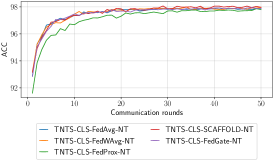
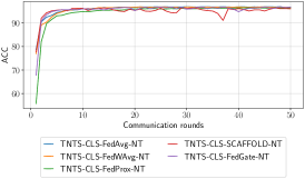
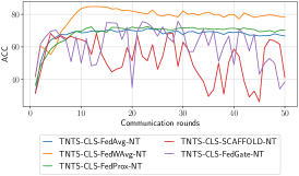
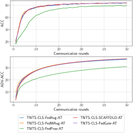
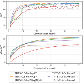
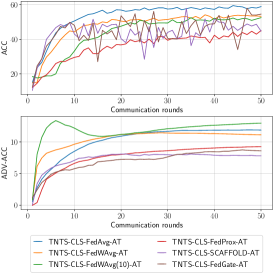
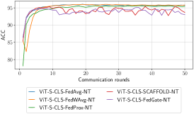
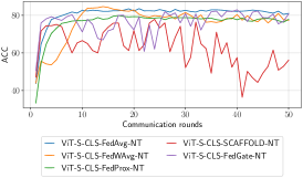
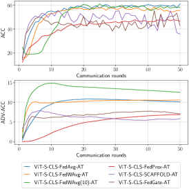
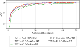
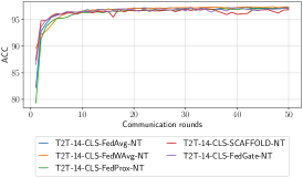
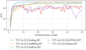
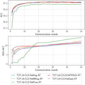
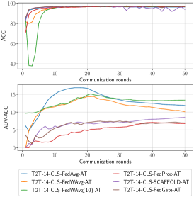
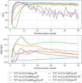
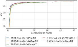
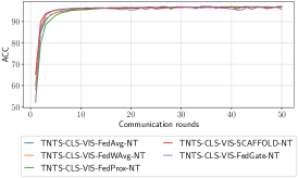
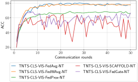
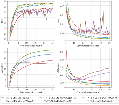
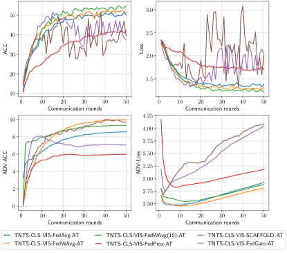
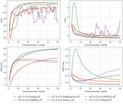
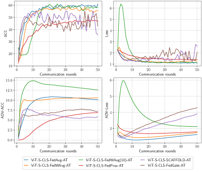
FedWAvg convergence. Fig. 2 shows the accuracy and robust accuracy of TNT-CLS model in the FL and FAT processes, respectively, with different aggregation methods. Similar figures with loss values for other models are in App. C. In federated natural training with IID and Non-IID(4) data distributions as shown in Fig. 2a and Fig. 2b, we notice that all the aggregation methods yield a fast convergence roughly from round 2. Unlike other methods, FedProx needs more rounds to reach a comparable accuracy performance to other methods. FedWAvg shows comparable and stable convergence behavior to other methods. While with Non-IID(2) data distribution as shown in Fig. 2c, FedWAvg shows comparable convergence, better for some models, to FedAvg. FedProx shows slow convergence while FedGate and SCAFFOLD show unstable convergence.

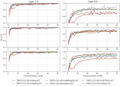
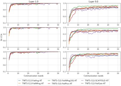
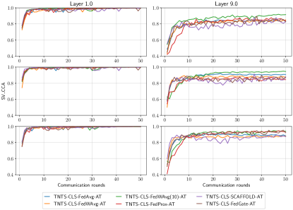
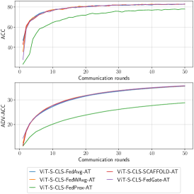
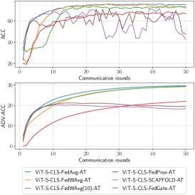
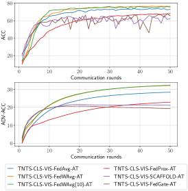
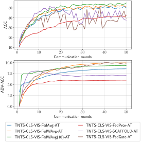
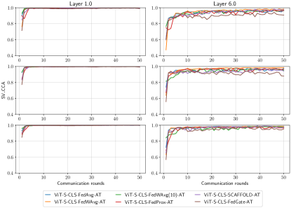
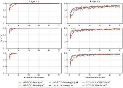
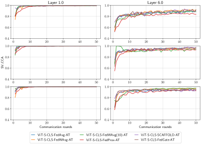
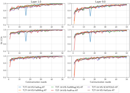
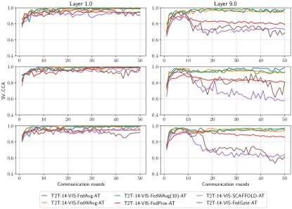
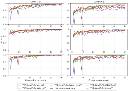
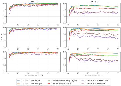
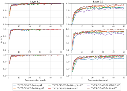
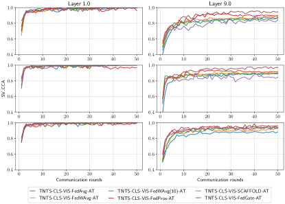
In FAT with IID data distribution as shown in Fig. 2d, FedWAvg shows comparable convergence to other methods while FedProx shows slow convergence. With Non-IID(4) and Non-IID(2) data distributions as shown in Fig. 2e and Fig. 2f, FedGate and SCAFFOLD show unstable convergence for the accuracy and show slow convergence for the robust accuracy. Moreover, FedProx shows slow convergence for robust accuracy, while FedWAvg shows comparable or better convergence than FedAvg for robust accuracy. Moreover, we calculate the model drift using singular vector canonical correlation analysis (SV-CCA) (Raghu et al., 2017), as shown in Fig. 3, between client 1 and client 4 (top), between client 1 and the server (middle), and between client 4 and the server (bottom) for layer 1 and layer 9 of TNT-CLS model. In Fig. 3a, the SV-CCA is calculated using clean samples, while in Fig. 3b the SV-CCA is calculated using the adversarial samples. Similar figures for other models are given in App. D. We found that at layer 1, the drift between the clients and the server is decreasing during the training and all methods show comparable behavior. While at layer 9, the drift behavior of FedGate and SCAFFOLD is not stable as in FedAvg and FedWAvg.

Accuracy and robust accuracy with FedWAvg. For CNNs, the aggregation methods for FL are mainly developed and tested in the natural federated learning process. In this work we test the state-of-the-art aggregation methods in the FAT process for transformers. Tab. 1, Tab. 2, and Tab. 3 show the best accuracy for the natural federated learning and the best robust accuracy and the corresponding accuracy for the FAT with IID, Non-IID(4), and Non-IID(2) data distributions.

In federated natural training with IID and Non-IID(4), all aggregation methods including FedWAvg yield comparable model accuracy, while with Non-IID(2), FedProx, FedGate, and SCAFFOLD achieve less model accuracy compared to FedAvg. On the other hand, FedWAvg achieves better accuracy than FedAvg for models like T2T-ViT-VIS and TNT-CLS, and achieves comparable accuracy for models like T2T-ViT-CLS and ViT-B, and achieves less accuracy for models like T2T-ViT-CLS+VIS.

For the FAT process, we demonstrate the performance of the FedWAvg with the Non-IID data partitioning. With Non-IID(4), we notice that FedWAvg always yields better robust accuracy than FedProx, FedGate, and SCAFFOLD. Compared to FedAvg, we notice that FedWAvg yields better robust accuracy like in TNT-CLS-VIS and ViT-B, comparable robust accuracy like in ViT-CLS, and lower robust accuracy than FedAvg like in T2T-ViT-CLS. While with Non-IID(2), FedWAvg yields better robust accuracy than other aggregation methods with all models except with FedAvg in TNT-VIS model.

Table 1: Models accuracy under NT and models (accuracy, robust accuracy) under AT in FL with IID. The first and the second best robust accuracy are marked.

Architecture			FedAvg		FedProx		FedGate		SCAFFOLD		FedWAvg(1)
Token	Model	Class. Head	NT	AT	NT	AT	NT	AT	NT	AT	NT	AT
Image patch	VIT-S	CLS	97.35	(82.73, 35.57)	97.14	(77.96, 28.82)	97.35	(82.91, 35.76)	97.46	(83.01, 35.71)	97.33	(82.91, 35.67)
		VIS	97.31	(81.04, 34.9)	97.2	(75.70, 28.06)	97.31	(81.55, 35.13)	97.35	(81.31, 35.16)	97.26	(81.26, 34.79)
		CLS+VIS	97.25	(82.9, 35.82)	97.12	(78.05, 29.03)	97.36	(83.11, 36.05)	97.41	(82.92, 35.71)	97.27	(82.49, 35.83)
	VIT-B	CLS	98.71	(96.87. 28.01)	98.67	(97.41, 21.3)	98.82	(97.30, 26.84)	98.77	(97.27, 28.3)	98.76	(96.98, 25.77)
		VIS	98.7	(97.03, 22.79)	98.66	(98.16, 8.90)	98.74	(97.12, 25.63)	98.74	(97.01, 23.23)	98.74	(96.90, 20.98)
		CLS+VIS	98.73	(97.14, 29.79)	98.71	(97.22, 20.89	98.81	(97.18, 27.82)	98.81	(97.27, 29.07)	98.81	(97.04, 28.02)
T2T	T2T-14	CLS	98.14	(97.79, 11.07)	97.89	(96.87, 14.2)	98.09	(97.69, 11.79)	98.09	(97.87, 11.04)	98.11	(97.670, 12.41)
		VIS	97.99	(98.05, 9.0)	97.94	(97.72, 7.81)	98.07	(98.14, 8.9)	98.08	(98.15, 9.37)	97.93	(98.03, 8.67)
		CLS+VIS	98.07	(96.97, 14.52)	97.97	(96.97, 10.73	98.09	(97.37, 15.85)	98.07	(97.13, 16.07)	98.12	(97.04, 15.49)
TNT	TNT-S	CLS	97.92	(83.50, 36.93)	97.87	(79.64, 30.96)	97.93	(83.82, 37.27)	98.07	(84.07, 37.43)	97.97	(83.57, 37.41)
		VIS	97.82	(81.57, 35.88)	97.67	(74.19, 29.11)	97.84	(82.19, 35.89)	97.81	(82.49, 36.01)	97.79	(79.95, 34.58)
		CLS+VIS	97.95	(80.44, 35.17)	97.81	(75.02, 28.80)	98.07	(82.24, 36.28)	97.99	(82.27, 36.22)	98.02	(79.27, 34.09)

Table 2: Models accuracy under NT and models (accuracy, robust accuracy) under AT in FL with Non-IID(4). The first and the second best robust accuracy are marked.

Architecture			FedAvg		FedProx		FedGate		SCAFFOLD		FedWAvg(1)		FedWAvg(10)
Token	Model	Class. Head	NT	AT	NT	AT	NT	AT	NT	AT	NT	AT	NT	AT
Image patch	VIT-S	CLS	96.05	(75.18, 29.62)	95.62	(66.85, 22.01)	95.16	(71.04, 21.04)	95.41	(68.34, 20.25)	96	(71.94, 29.21)	-	(73.32, 29.37)
		VIS	95.98	(76.17, 31.09)	95.62	(67.86, 24.09)	95.45	(68.21, 20.89)	94.68	(71.67, 23.83)	96.02	(74.96, 30.43)	-	(76.43, 29.4)
		CLS+VIS	96.07	(75.91, 29.9)	95.66	(68.39, 22.27)	94.99	(69.91, 21.38)	95.46	(64.20, 19.69)	95.95	(75.18, 29.57)	-	(74.59, 29.2)
	VIT-B	CLS	98.45	(95.55, 14.41)	98.27	(96.57, 7.47)	98.49	(96.46, 3.97)	98.41	(97.37, 14.50)	98.42	(95.93, 17.6)	-	(96.15, 21.11)
		VIS	98.4	(96.06, 14.09)	98.33	(96.33, 11.11)	98.52	(96.75, 10.16)	98.32	(97.08, 10.39)	98.42	(96.09, 18.63)	-	(95.870, 17.93)
		CLS+VIS	98.33	(95.87, 19.82)	98.25	(96.35, 11.11)	98.32	(96.92, 11.39)	98.51	(96.91, 7.61)	98.47	(96.13, 22.36)	-	(95.43, 18.92)
T2T	T2T-14	CLS	97.29	(96.36, 16.89)	97.1	(96.79, 7.12)	97.25	(97.06, 7.52)	97.03	(93.87, 8.55)	97.41	(96.77, 14.40)	-	(96.70, 15.14)
		VIS	97.26	(97.51, 9.12)	97.13	(96.72, 8.66)	96.95	(97.41, 6.81)	97.12	(95.64, 6.8)	97.07	(97.49, 10.22)	-	(97.54, 8.97)
		CLS+VIS	97.22	(96.31, 15.65)	97.11	(96.30, 8.04)	97.14	(96.11, 8.75)	97	(95.67, 9.33)	97.46	(96.38, 10.94)	-	(96.13, 13.99)
TNT	TNT-S	CLS	96.96	(74.84, 31.94)	96.53	(70.34, 22.76)	97.02	(70.99, 22.13)	96.51	(71.35, 28.44)	96.93	(75.68, 32.39)	-	(74.43, 31.03)
		VIS	96.7	(75.71, 32.6)	96.41	(61.21, 19.12)	96.59	(61.32, 19.39)	96.52	(66.23, 22.19)	96.65	(74.26, 30.85)	-	(75.91, 31.83)
		CLS+VIS	96.99	(73.04, 28.42)	96.91	(68.29, 22.87)	96.81	(66.44, 20.66)	97.1	(65.460, 21.5)	96.77	(76.36, 32.34)	-	(75.70. 32.16)

Table 3: Models accuracy under NT and models (accuracy, robust accuracy) under AT in FL with Non-IID(2). The first and the second best robust accuracy are marked.

Architecture			FedAvg		FedProx		FedGate		SCAFFOLD		FedWAvg(1)		FedWAvg(10)
Token	Model	Class. Head	NT	AT	NT	AT	NT	AT	NT	AT	NT	AT	NT	AT
Image patch	VIT-S	CLS	83.52	(58.51, 10.83)	79.86	(46.70, 6.89)	82.92	(55.41, 7.62)	77.88	(53.28, 7.78)	84.62	(58.44, 10.52)	-	(58.20, 14.01)
		VIS	82.56	(61.31, 13.36)	73.46	(51.02, 7.51)	75.61	(48.71, 7.34)	73.44	(50.12, 7.65)	80.49	(57.63, 11.45)	-	(58.28, 13.3)
		CLS+VIS	85.03	(58.63, 10.19)	80.89	(46.11, 8.76)	80.64	(47.17, 9.33)	78.91	(51.4, 6.10)	86.49	(59.36, 9.76)	-	(54.75, 11.1)
	VIT-B	CLS	96.43	(87.81, 4.96)	94.88	(82.04, 1.2)	94.51	(90.64, 3.15)	94.89	(90.17, 6.68)	96.7	(86.56, 8.10)	-	(83.62, 13.79)
		VIS	96.72	(83.76, 5.91)	96.24	(80.69, 3.04)	95.23	(89.18, 2.45)	94.86	(88.99, 3.85)	97.15	(90.49, 8.95)	-	(90.61, 12.22)
		CLS+VIS	96.42	(83.95, 7.26)	95.7	(82.62, 2.48)	95.38	(91.39, 4.81)	93.23	(88.15, 5.69)	96.48	(86.90, 7.61)	-	(84.68, 14.09)
T2T	T2T-14	CLS	92.1	(85.6, 1.88)	89.45	(83.10, 4.83)	87	(86.65, 5.93)	86.87	(83.02, 3.90)	92.12	(83.66, 7.08)	-	(80.77, 8.75)
		VIS	81.8	(84.75, 3.59)	81.45	(80.84, 2.84)	72.1	(80.26, 5.04)	79.2	(79.19, 2.99)	84.84	(82.31, 6.87)	-	(87.66, 9.33)
		CLS+VIS	90.81	(83.47, 5.28)	83.77	(79.43, 1.40)	88.5	(81.79, 4.52)	88.9	(80.42, 6.07)	85.47	(78.32, 6.28)	-	(79.02, 7.32)
TNT	TNT-S	CLS	71.31	(57.69, 11.89)	72.5	(45.01, 9.25)	75.81	(58.01, 8.68)	68.43	(51.78, 8.00)	84.78	(50.94, 11.43)	-	(52.51, 12.96)
		VIS	64.11	(59.23, 12.08)	66.04	(44.73, 5.8)	63.39	(50.64, 6.3)	59.42	(47.75, 5.9)	60.45	(54.88, 9.97)	-	(51.45, 9.97)
		CLS+VIS	80.3	(50.09, 8.56)	68.81	(42.13, 5.96)	68.19	(51.77, 9.59)	64.67	(46.09, 8.07)	78.77	(50.98, 9.94)	-	(53.66, 9.31)

Robustness and tokenization. Tokenization played an important role in the FL and the FAT processes. As shown in Tab. 1, Tab. 2, and Tab. 3, tokens-to-token method has positive role in enhancing the models’ accuracies in NT and AT process when compared with size-comparable vision transformer ViT-S and TNT-S, while it has negative role in enhancing models’ robust accuracies. Tokens-to-token method showed its ability to represent training samples with local and global features that helps enhancing the model accuracy. The main reason for the low robust accuracy is as mentioned in (Aldahdooh et al., 2021); the energy spectrum of the perturbation that is generated using PGD for the T2T-ViT model is not spread across all frequencies which makes T2T-ViT not robust against the PGD attack. On the other hand, image patches in ViT-S and mapping local pixel dependencies of image patches in TNT models don’t help with Non-IID data partitioning. With Non-IID(4), ViT-S and TNT show comparable performance that decrease model’s accuracy and increase the model’s robust accuracy. While with Non-IID(2) ViT shows better model’s accuracy in NT and in AT process. As a conclusion, you can select the tokenization method according to the priority you give to accuracy and robust accuracy.

Robustness and classification head. The role of the classification head type appears during the NT process with Non-IID(2) data partitioning. We notice, as shown in Tab. 3, that using VIS tokens only for the classification head notably decreases model’s accuracy, while using CLS token only for the classification head significantly enhance the modle’s accuracy. Compared to using CLS token, combining both configurations, i.e. CLS+VIS, may yield better model’s accuracy like in TNT with FedAvg, or may yield lower model’s accuracy like in T2T-ViT with FedWAvg.

Moreover, the role of the classification head type appears during the AT process with IID and Non-IID data partitioning. With the IID data distribution, as shown in Tab. 1, using CLS token for the classification head enhances the model’s accuracy and the model’s robust accuracy in TNT models, while using VIS tokens for the classification head decreases the model’s robust accuracy in T2T-ViT models. With the Non-IID, the preference of one classification head type is not clear. Finally, we can conclude that avoid using VIS tokens alone for the classification head is recommended.

ViT-S and ViT-B. We notice that the ViT-B significantly enhances the model accuracy and fails in enhancing the robust accuracy with IID and Non-IID(4). While with Non-IID, ViT-B achieves comparable robust accuracy to ViT-S. Hence, we recommend, for high heterogeneous data partitioning, to use ViT model with large number of attention blocks.

5 Conclusion

In this work, we studied the feasibility of AT in a FL process for vision transformers. Vision transformer models that have different tokenization and classification head techniques were investigated with different federated model aggregation methods. We found that the state-of-the-art aggregation methods decrease the robust accuracy of the model compared to FedAvg with Non-IID. Hence, we proposed an extension to the FedAvg algorithm, called FedWAvg, to improve the robust accuracy of the model. We showed that FedWAvg improved the robust accuracy with highly heterogeneous data and has comparable convergence and drift behavior compared to FedAvg. Moreover, we showed that choosing the tokenization method depends on the system’s goal of either enhancing the model’s accuracy or enhancing the model’s robust accuracy. Finally we showed that it is recommended to avoid using visual tokens alone for the classification head.

Appendix A Vision Transformers

In this section, we briefly show the related work that belongs to transformers and then we show the different models that we consider in our experiments, as described in Fig. 4.

A.1 Related work

Transformer (Vaswani et al., 2017) was first introduced for natural language processing (NLP) tasks. It adopts the self-attention mechanism to learn the model. Transformer and its variants maintain state-of-the-art performance for different NLP tasks. Recently, transformers were found to be effective for different computer vision tasks, such as, image processing (Chen et al., 2021b), video processing (Cao et al., 2021), and image classification (Dosovitskiy et al., 2021). Dosovitskiy et al. (Dosovitskiy et al., 2021) was the first to build an image classification model, vision transformer (ViT), that uses the vanilla transformer encoder blocks. ViT and its variants establish the state-of-the-art performance especially if it is trained with significantly large-scale datasets, such as JFT-300M (Sun et al., 2017; Dosovitskiy et al., 2021). Using transfer learning, ViT models can be downgraded to smaller datasets, such as ImageNet-1k (Deng et al., 2009), and achieves performance comparable to or better than state-of-the-art CNNs models. Recently, in (Qu et al., 2021), Qu et al. investigated the feasibility of using ViTs in the FL settings and observed that ViTs significantly accelerate convergence and reach a better global model, especially when dealing with heterogeneous data.

ViT has the capability to learn the global context of the input image, while it is not effectively capable to learn local features as CNNs and that’s why ViT requires large-scale dataset for training to maintain the state-of-the-art performance. Hence, many efforts have been done to mitigate this obstacle (Dosovitskiy et al., 2021; Yuan et al., 2021; Han et al., 2021; Xie et al., 2021). One approach is the embedding based approach in which the way of generating the embedded patches to be passed to the transformer encoder is changed. In (Dosovitskiy et al., 2021), ViT-Res is introduced which replaces the input image patches with the flattened ResNet-50 feature maps to generate the embedded patches. While in (Yuan et al., 2021), tokens-to-token ViT (T2T-ViT) replaces input image patches with a tokens-to-token (T2T) transformation. The T2T module progressively structurizes the image into tokens by recursively aggregating neighboring tokens into one token. The features that are learned by the T2T module are, then, passed to the transformer encoder. In (Han et al., 2021), Han et al. suggested to model both patch-level and pixel-level representations and proposed transformer-in-transformer (TNT) architecture. It stacks multiple TNT blocks that each has an inner transformer and an outer transformer. The inner transformer block further divides the image patch to sub-patches to extract local features from pixel embeddings. The output of the inner transformer block is merged with the patch embeddings to be the input of the outer transformer block. Other architectures exist in the literature like convolutional vision transformer (CvT) (Wu et al., 2021) and conditional position encoding vision transformer (CPVT) (Chu et al., 2021). Another approach to mitigate the ViT obstacle is to customize the classification head of the model. ViT only uses the class token for the classification while second-order vision transformer (So-ViT) (Xie et al., 2021) uses visual tokens along with the class token. So-ViT proposes a second-order cross-covariance pooling of visual tokens to be combined with the class token for final classification. Moreover the work in (Mao et al., 2021b) considered only the visual tokens.

A.2 Vision Transformer Models

ViT’s encoder receives as input a 1D sequence of token embeddings. The image $\mathbf{x}\in\mathbb{R}^{H\times W\times C}$ is reshaped into a sequence of flattened 2D image patches $\mathbf{x}_{p}\in\mathbb{R}^{N\times(P^{2}\times C)}$, where $H,W,C,P,\text{ and }N$ are image height, image width, number of image channels, patch width and height, and $N=\frac{HW}{P^{2}}$ is the number of patches, respectively. To prepare the patch embeddings, Eq. 4, the flattened patches are mapped to $D$ dimensions with a trainable linear projection since the transformer encoder uses constant latent vector size $D$ for all the layers. To maintain the positional information, Eq. 4, position embeddings are added to the patch embeddings using the standard learnable 1D position embeddings. The basic component in the transformer-based neural networks is the attention blocks. The standard transformer encoder in ViT stacks $L$ layers of attention blocks. The attention block consists of two sub-layers; the first is the multiheaded self-attention (MSA), Eq. 5, and the second is a simple multi-layer perceptron (MLP) layer, Eq. 6, also called position-wise fully connected feed-forward network (FFN). Layernorm (LN) is applied before every sub-layer, and residual connections are applied after each sub-layer. mlp consists of two linear transformation layers and a nonlinear activation function, Gaussian error linear units (GELU) (Hendrycks & Gimpel, 2016), in between. For classification head, ViT adds [CLS] token to the sequence of embedded patches ($\mathbf{z}_{0}^{0}=\mathbf{x}_{class}$). The [CLS] token at the transformer’s output $\mathbf{z_{L}^{0}}$ will be used for image representation, Eq. 7.

$$\begin{gathered}\mathbf{z}_{0}=[\mathbf{x}_{class};\mathbf{x}_{p}^{1}\mathbf{E};\mathbf{x}_{p}^{2}\mathbf{E};\dots;\mathbf{x}_{p}^{N}\mathbf{E}]+\mathbf{E}_{pos},\\ \mathbf{E}\in\mathbb{R}^{(P^{2}\times C)\times D},\text{ }\mathbf{E}_{pos}\in\mathbb{R}^{(N+1)\times D}\end{gathered}$$ (4)

$$\begin{gathered}\mathbf{z}_{l}^{\prime}=MSA(LN(\mathbf{z}_{l-1}))+\mathbf{z}_{l-1},\text{ }l=1\dots L\end{gathered}$$ (5)

$$\begin{gathered}\mathbf{z}_{l}=MLP(LN(\mathbf{z}_{l}^{\prime}))+\mathbf{z}_{l}^{\prime},\text{ }l=1\dots L\end{gathered}$$ (6)

$$\begin{gathered}\mathbf{y}=LN(\mathbf{z}_{L}^{0})\end{gathered}$$ (7)

Figure 4: Tested Vision Transformers’ Architectures for Federated Adversarial Training. The left part shows the main blocks of the transformer. 1) The embedded patches block. 2) the Attention block, and 3) the classification head block. For the embedding patches, we consider three methods, in green blocks, a) image patches, tokens-to-token, and sub-patches for image patches. For the Attention block, we consider the multi-head attention mechanism. For the classification head block, we consider using the CLS token, VIS tokens, and both.

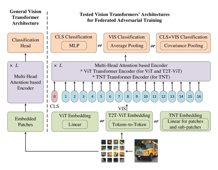
Other patch embeddings methods. As discussed earlier in Sec. A.1, T2T-ViT replaces input image patches with a tokens-to-token (T2T) transformation (Yuan et al., 2021). The T2T module progressively structurizes the image into tokens by recursively aggregating neighboring tokens into one token. The features that are learned by the T2T module are, then, passed to the transformer encoder. While TNT (Han et al., 2021) models both patch-level and pixel-level representations. It stacks multiple TNT blocks that each has an inner transformer and an outer transformer. The inner transformer block further divides the image patch to sub-patches to extract local features from pixel embeddings. The output of the inner transformer block is merged with the patch embeddings to be the input of the outer transformer block.

Figure 5: The classification head that is proposed in (Xie et al., 2021) that uses the second-order cross-covariance pooling of visual tokens. FC: fully connected layer.

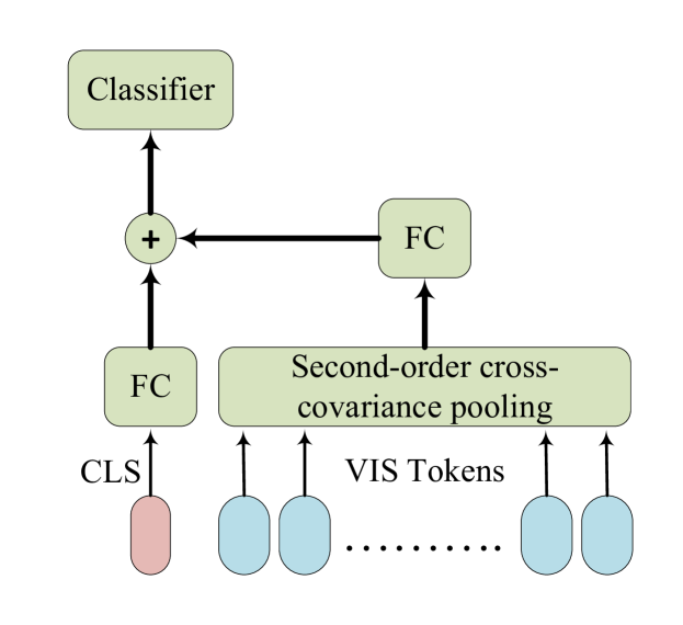
Other classification head methods. In order to improve vision transformer robustness, the work (Mao et al., 2021b) suggested a classification head that depends on the visual tokens [$\mathbf{z}_{L}^{1\dots N}$] not on the [CLS] token $\mathbf{z}_{L}^{0}$. The proposed classification head performs average pooling of the visual tokens. While the work in (Xie et al., 2021) proposed a classification head that depends on class and visual tokens as illustrated in Fig. 5 in order to improve the network accuracy.

In summary, we investigate the vision transformer models with three different embedding methods and three different classification head methods. Fig. 4 illustrates the models’ architectures. For ViT embedding, we use ViT-S-16 and ViT-B-16 models. For T2T-ViT embedding, we use T2T-ViT-14 and finally, for TNT embedding, we use the TNT-S model. For these four models, three classification heads are used; the first uses the class [CLS] token only, the second uses the visual [VIS] tokens only, and the third uses both the [CLS] and the [VIS] tokens. In total we tested 12 vision transformer models.

Appendix B More figures cosine similarity weights

More figures to show the calculated cosine similarity weights for some of the tested models are shown in Figs. 6, 7, 8, 9 and 10

(a)

(b)

Figure 6: The calculated weights using cosine similarity, Eq. 3 during the federated training process using ViT-S model and IID partitioning. a) for the natural training, and b) for the adversarial training.

(a)

(b)

Figure 7: The calculated weights using cosine similarity, Eq. 3 during the federated training process using ViT-S model and Non-IID partitioning (each client has 4 classes). a) for the natural training, and b) for the adversarial training.

(a)

(b)

Figure 8: The calculated weights using cosine similarity, Eq. 3 during the federated training process using ViT-S model and Non-IID partitioning (each client has 2 classes). a) for the natural training, and b) for the adversarial training.

(a)

(b)

Figure 9: The calculated weights using cosine similarity, Eq. 3 during the federated training process using T2T-ViT-14-VIS model and Non-IID partitioning (each client has 4 classes). a) for the natural training, and b) for the adversarial training.

(a)

(b)

Figure 10: The calculated weights using cosine similarity, Eq. 3 during the federated training process using TNT-S-CLS+VIS model and Non-IID partitioning (each client has 4 classes). a) for the natural training, and b) for the adversarial training.

Appendix C More figures for FedWAvg convergence

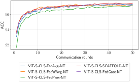
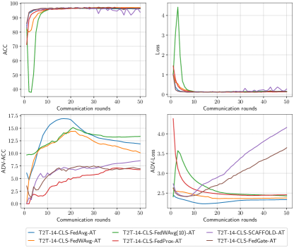
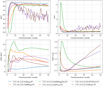
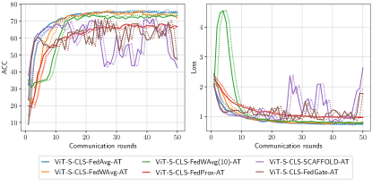
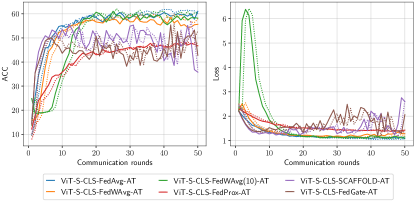
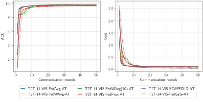
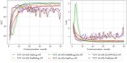
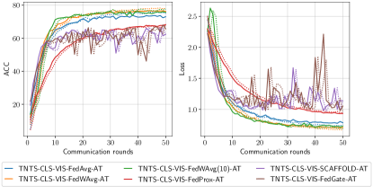
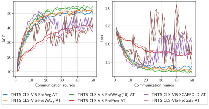
More figures to show the convergence of FedWAvg and some of the tested state-of-the-art are shown in Figs. 11, 12 and 13. Other figures that shows the convergence and the loss are shown in Figs. 14, 15 and 16. Moreover, Figs. 17, 17 and 19 show the convergence during the training and the testing.

(a)

(b)

(c)

(d)

(e)

(f)

Figure 11: The accuracy and robust accuracy of ViT-S-CLS model in the FAT process for different aggregation methods. The accuracies against the communication rounds under the NT process using IID, Non-IID(4), and Non-IID(2) are shown in a), b), and c) respectively. The accuracies (top) and the robust accuracies (bottom) against the communication rounds under the AT process using IID, Non-IID(4), and Non-IID(2) are shown in d), e), and f) respectively.

(a)

(b)

(c)

(d)

(e)

(f)

Figure 12: The accuracy and robust accuracy of T2T-ViT-CLS model in the FAT process for different aggregation methods. The accuracies against the communication rounds under the NT process using IID, Non-IID(4), and Non-IID(2) are shown in a), b), and c) respectively. The accuracies (top) and the robust accuracies (bottom) against the communication rounds under the AT process using IID, Non-IID(4), and Non-IID(2) are shown in d), e), and f) respectively.

(a)

(b)

(c)

(d)

(e)

(f)

Figure 13: The accuracy and robust accuracy of TNT-CLS+VIS model in the FAT process for different aggregation methods. The accuracies against the communication rounds under the NT process using IID, Non-IID(4), and Non-IID(2) are shown in a), b), and c) respectively. The accuracies (top) and the robust accuracies (bottom) against the communication rounds under the AT process using IID, Non-IID(4), and Non-IID(2) are shown in d), e), and f) respectively.

(a)

(b)

Figure 14: The accuracy and the robust accuracy of TNT-CLS+VIS model with loss values in the FAT process for different aggregation methods. The accuracies (top) and the robust accuracies (bottom) against the communication rounds under the AT process using Non-IID(4), and Non-IID(2) are shown in a), and b) respectively.

(a)

(b)

Figure 15: The accuracy and the robust accuracy of ViT-CLS model with loss values in the FAT process for different aggregation methods. The accuracies (top) and the robust accuracies (bottom) against the communication rounds under the AT process using Non-IID(4), and Non-IID(2) are shown in a), and b) respectively.

(a)

(b)

Figure 16: The accuracy and the robust accuracy of T2T-ViT-CLS model with loss values in the FAT process for different aggregation methods. The accuracies (top) and the robust accuracies (bottom) against the communication rounds under the AT process using Non-IID(4), and Non-IID(2) are shown in a), and b) respectively.

(a)

(b)

Figure 17: The accuracy in training (dashed) and testing (solid) of ViT-CLS model with loss values in the FAT process for different aggregation methods. The accuracies against the communication rounds under the AT process using Non-IID(4), and Non-IID(2) are shown in a), and b) respectively. For better visualization dashed line is shifted for one round forward.

(a)

(b)

Figure 18: The accuracy in training (dashed) and testing (solid) of T2T-ViT-VIS model with loss values in the FAT process for different aggregation methods. The accuracies against the communication rounds under the AT process using Non-IID(4), and Non-IID(2) are shown in a), and b) respectively. For better visualization dashed line is shifted for one round forward.

(a)

(b)

Figure 19: The accuracy in training (dashed) and testing (solid) of TNT-CLS+VIS model with loss values in the FAT process for different aggregation methods. The accuracies against the communication rounds under the AT process using Non-IID(4), and Non-IID(2) are shown in a), and b) respectively. For better visualization dashed line is shifted for one round forward.

Appendix D More figures for model drift

Figs. 20, 21, 22, 23, 24 and 25 show more model drift for some of the tested models.

(a) With clean samples

(b) With adversarial samples

Figure 20: The SV-CCA for the first and the ninth layer of server, client 1, and client 4 models against communication rounds under FAT process using ViT-CLS model with Non-IID(4). a) using clean test samples and b) using adversarial test samples. The top row shows the SV-CCA between client 1 and client 2, the middle row shows the SV-CCA between the server and client 1, and the bottom row shows the SV-CCA between the server and client 4.

(a) With clean samples

(b) With adversarial samples

Figure 21: The SV-CCA for the first and the ninth layer of server, client 1, and client 4 models against communication rounds under FAT process using ViT-CLS model with Non-IID(2). a) using clean test samples and b) using adversarial test samples. The top row shows the SV-CCA between client 1 and client 2, the middle row shows the SV-CCA between the server and client 1, and the bottom row shows the SV-CCA between the server and client 4.

(a) With clean samples

(b) With adversarial samples

Figure 22: The SV-CCA for the first and the ninth layer of server, client 1, and client 4 models against communication rounds under FAT process using T2T-ViT-VIS model with Non-IID(4). a) using clean test samples and b) using adversarial test samples. The top row shows the SV-CCA between client 1 and client 2, the middle row shows the SV-CCA between the server and client 1, and the bottom row shows the SV-CCA between the server and client 4.

(a) With clean samples

(b) With adversarial samples

Figure 23: The SV-CCA for the first and the ninth layer of server, client 1, and client 4 models against communication rounds under FAT process using T2T-ViT-VIS model with Non-IID(2). a) using clean test samples and b) using adversarial test samples. The top row shows the SV-CCA between client 1 and client 2, the middle row shows the SV-CCA between the server and client 1, and the bottom row shows the SV-CCA between the server and client 4.

(a) With clean samples

(b) With adversarial samples

Figure 24: The SV-CCA for the first and the ninth layer of server, client 1, and client 4 models against communication rounds under FAT process using TNT-CLS-VIS model with Non-IID(4). a) using clean test samples and b) using adversarial test samples. The top row shows the SV-CCA between client 1 and client 2, the middle row shows the SV-CCA between the server and client 1, and the bottom row shows the SV-CCA between the server and client 4.

(a) With clean samples

(b) With adversarial samples

Figure 25: The SV-CCA for the first and the ninth layer of server, client 1, and client 4 models against communication rounds under FAT process using TNT-CLS-VIS model with Non-IID(2). a) using clean test samples and b) using adversarial test samples. The top row shows the SV-CCA between client 1 and client 2, the middle row shows the SV-CCA between the server and client 1, and the bottom row shows the SV-CCA between the server and client 4.

References

- Akhtar et al. (2021) Akhtar, N., Mian, A., Kardan, N., and Shah, M. Threat of adversarial attacks on deep learning in computer vision: Survey II. CoRR, abs/2108.00401, 2021. URL https://arxiv.org/abs/2108.00401.
- Aldahdooh et al. (2021) Aldahdooh, A., Hamidouche, W., and Déforges, O. Reveal of vision transformers robustness against adversarial attacks. CoRR, abs/2106.03734, 2021. URL https://arxiv.org/abs/2106.03734.
- Aldahdooh et al. (2022) Aldahdooh, A., Hamidouche, W., Fezza, S. A., and Déforges, O. Adversarial example detection for dnn models: A review and experimental comparison. Artificial Intelligence Review, 2022. URL https://doi.org/10.1007/s10462-021-10125-w.
- Bai et al. (2021) Bai, T., Luo, J., Zhao, J., Wen, B., and Wang, Q. Recent advances in adversarial training for adversarial robustness. In Proceedings of the Thirtieth International Joint Conference on Artificial Intelligence, IJCAI 2021, Virtual Event / Montreal, Canada, 19-27 August 2021, pp. 4312–4321. ijcai.org, 2021. doi: 10.24963/ijcai.2021/591. URL https://doi.org/10.24963/ijcai.2021/591.
- Basu et al. (2020) Basu, D., Data, D., Karakus, C., and Diggavi, S. N. Qsparse-local-sgd: Distributed sgd with quantization, sparsification, and local computations. IEEE Journal on Selected Areas in Information Theory, 1(1):217–226, 2020.
- Blanchard et al. (2017) Blanchard, P., Mhamdi, E. M. E., Guerraoui, R., and Stainer, J. Machine learning with adversaries: Byzantine tolerant gradient descent. In Advances in Neural Information Processing Systems 30: Annual Conference on Neural Information Processing Systems 2017, December 4-9, 2017, Long Beach, CA, USA, pp. 119–129, 2017. URL https://proceedings.neurips.cc/paper/2017/hash/f4b9ec30ad9f68f89b29639786cb62ef-Abstract.html.
- Cao et al. (2021) Cao, J., Li, Y., Zhang, K., and Gool, L. V. Video super-resolution transformer. CoRR, abs/2106.06847, 2021. URL https://arxiv.org/abs/2106.06847.
- Chen et al. (2021a) Chen, C., Kailkhura, B., Goldhahn, R. A., and Zhou, Y. Certifiably-robust federated adversarial learning via randomized smoothing. CoRR, abs/2103.16031, 2021a. URL https://arxiv.org/abs/2103.16031.
- Chen et al. (2021b) Chen, H., Wang, Y., Guo, T., Xu, C., Deng, Y., Liu, Z., Ma, S., Xu, C., Xu, C., and Gao, W. Pre-trained image processing transformer. In IEEE Conference on Computer Vision and Pattern Recognition, CVPR 2021, virtual, June 19-25, 2021, pp. 12299–12310. Computer Vision Foundation / IEEE, 2021b. URL https://openaccess.thecvf.com/content/CVPR2021/html/Chen_Pre-Trained_Image_Processing_Transformer_CVPR_2021_paper.html.
- Chen et al. (2020) Chen, T., Kornblith, S., Norouzi, M., and Hinton, G. E. A simple framework for contrastive learning of visual representations. In Proceedings of the 37th International Conference on Machine Learning, ICML 2020, 13-18 July 2020, Virtual Event, volume 119 of Proceedings of Machine Learning Research, pp. 1597–1607. PMLR, 2020. URL http://proceedings.mlr.press/v119/chen20j.html.
- Chu et al. (2021) Chu, X., Zhang, B., Tian, Z., Wei, X., and Xia, H. Do we really need explicit position encodings for vision transformers? CoRR, abs/2102.10882, 2021. URL https://arxiv.org/abs/2102.10882.
- Defazio et al. (2014) Defazio, A., Bach, F. R., and Lacoste-Julien, S. SAGA: A fast incremental gradient method with support for non-strongly convex composite objectives. In Advances in Neural Information Processing Systems 27: Annual Conference on Neural Information Processing Systems 2014, December 8-13 2014, Montreal, Quebec, Canada, pp. 1646–1654, 2014. URL https://proceedings.neurips.cc/paper/2014/hash/ede7e2b6d13a41ddf9f4bdef84fdc737-Abstract.html.
- Deng et al. (2009) Deng, J., Dong, W., Socher, R., Li, L.-J., Li, K., and Fei-Fei, L. Imagenet: A large-scale hierarchical image database. In 2009 IEEE conference on computer vision and pattern recognition, pp. 248–255. IEEE, 2009.
- Dong et al. (2021) Dong, Y., Fu, Q., Yang, X., Xiang, W., Pang, T., Su, H., Zhu, J., Tang, J., Chen, Y., Mao, X., He, Y., Xue, H., Li, C., Liu, Y., Zhang, Q., Gao, L., Yu, Y., Gao, X., Zhao, Z., Lin, D., Lin, J., Song, C., Wang, Z., Wu, Z., Guo, Y., Cui, J., Xu, X., and Chen, P. Adversarial attacks on ML defense models competition. CoRR, abs/2110.08042, 2021. URL https://arxiv.org/abs/2110.08042.
- Dosovitskiy et al. (2021) Dosovitskiy, A., Beyer, L., Kolesnikov, A., Weissenborn, D., Zhai, X., Unterthiner, T., Dehghani, M., Minderer, M., Heigold, G., Gelly, S., Uszkoreit, J., and Houlsby, N. An image is worth 16x16 words: Transformers for image recognition at scale. In 9th International Conference on Learning Representations, ICLR 2021, Virtual Event, Austria, May 3-7, 2021. OpenReview.net, 2021.
- Goodfellow et al. (2015) Goodfellow, I. J., Shlens, J., and Szegedy, C. Explaining and harnessing adversarial examples. In 3rd International Conference on Learning Representations, ICLR 2015, San Diego, CA, USA, May 7-9, 2015, Conference Track Proceedings, 2015.
- Haddadpour et al. (2021) Haddadpour, F., Kamani, M. M., Mokhtari, A., and Mahdavi, M. Federated learning with compression: Unified analysis and sharp guarantees. In The 24th International Conference on Artificial Intelligence and Statistics, AISTATS 2021, April 13-15, 2021, Virtual Event, volume 130 of Proceedings of Machine Learning Research, pp. 2350–2358. PMLR, 2021. URL http://proceedings.mlr.press/v130/haddadpour21a.html.
- Han et al. (2021) Han, K., Xiao, A., Wu, E., Guo, J., Xu, C., and Wang, Y. Transformer in transformer. CoRR, abs/2103.00112, 2021.
- He et al. (2016) He, K., Zhang, X., Ren, S., and Sun, J. Deep residual learning for image recognition. In Proceedings of the IEEE conference on computer vision and pattern recognition, pp. 770–778, 2016.
- Hendrycks & Gimpel (2016) Hendrycks, D. and Gimpel, K. Gaussian error linear units (GELUs). CoRR, abs/1606.08415, 2016.
- Hong et al. (2021) Hong, J., Wang, H., Wang, Z., and Zhou, J. Federated robustness propagation: Sharing adversarial robustness in federated learning. CoRR, abs/2106.10196, 2021. URL https://arxiv.org/abs/2106.10196.
- Imteaj et al. (2020) Imteaj, A., Thakker, U., Wang, S., Li, J., and Amini, M. H. Federated learning for resource-constrained IoT devices: Panoramas and state-of-the-art. CoRR, abs/2002.10610, 2020. URL https://arxiv.org/abs/2002.10610.
- Jere et al. (2020) Jere, M. S., Farnan, T., and Koushanfar, F. A taxonomy of attacks on federated learning. IEEE Security & Privacy, 19(2):20–28, 2020.
- Jiang et al. (2020) Jiang, J. C., Kantarci, B., Oktug, S., and Soyata, T. Federated learning in smart city sensing: Challenges and opportunities. Sensors, 20(21):6230, 2020.
- Johnson & Zhang (2013) Johnson, R. and Zhang, T. Accelerating stochastic gradient descent using predictive variance reduction. In Advances in Neural Information Processing Systems 26: 27th Annual Conference on Neural Information Processing Systems 2013. Proceedings of a meeting held December 5-8, 2013, Lake Tahoe, Nevada, United States, pp. 315–323, 2013. URL https://proceedings.neurips.cc/paper/2013/hash/ac1dd209cbcc5e5d1c6e28598e8cbbe8-Abstract.html.
- Kairouz et al. (2021) Kairouz, P., McMahan, H. B., Avent, B., Bellet, A., Bennis, M., Bhagoji, A. N., Bonawitz, K. A., Charles, Z., Cormode, G., Cummings, R., D’Oliveira, R. G. L., Eichner, H., Rouayheb, S. E., Evans, D., Gardner, J., Garrett, Z., Gascón, A., Ghazi, B., Gibbons, P. B., Gruteser, M., Harchaoui, Z., He, C., He, L., Huo, Z., Hutchinson, B., Hsu, J., Jaggi, M., Javidi, T., Joshi, G., Khodak, M., Konečný, J., Korolova, A., Koushanfar, F., Koyejo, S., Lepoint, T., Liu, Y., Mittal, P., Mohri, M., Nock, R., Özgür, A., Pagh, R., Qi, H., Ramage, D., Raskar, R., Raykova, M., Song, D., Song, W., Stich, S. U., Sun, Z., Suresh, A. T., Tramèr, F., Vepakomma, P., Wang, J., Xiong, L., Xu, Z., Yang, Q., Yu, F. X., Yu, H., and Zhao, S. Advances and open problems in federated learning. Found. Trends Mach. Learn., 14(1-2):1–210, 2021. doi: 10.1561/2200000083. URL https://doi.org/10.1561/2200000083.
- Karimireddy et al. (2020) Karimireddy, S. P., Kale, S., Mohri, M., Reddi, S. J., Stich, S. U., and Suresh, A. T. SCAFFOLD: stochastic controlled averaging for federated learning. In Proceedings of the 37th International Conference on Machine Learning, ICML 2020, 13-18 July 2020, Virtual Event, volume 119 of Proceedings of Machine Learning Research, pp. 5132–5143. PMLR, 2020. URL http://proceedings.mlr.press/v119/karimireddy20a.html.
- Krizhevsky & Hinton (2009) Krizhevsky, A. and Hinton, G. Learning multiple layers of features from tiny images. Master’s thesis, Department of Computer Science, University of Toronto, 2009.
- Kulkarni et al. (2020) Kulkarni, V., Kulkarni, M., and Pant, A. Survey of personalization techniques for federated learning. CoRR, abs/2003.08673, 2020. URL https://arxiv.org/abs/2003.08673.
- Kurakin et al. (2017) Kurakin, A., Goodfellow, I. J., and Bengio, S. Adversarial machine learning at scale. In 5th International Conference on Learning Representations, ICLR 2017, Toulon, France, April 24-26, 2017, Conference Track Proceedings. OpenReview.net, 2017. URL https://openreview.net/forum?id=BJm4T4Kgx.
- Li et al. (2019) Li, T., Sahu, A. K., Zaheer, M., Sanjabi, M., Talwalkar, A., and Smith, V. Federated optimization in heterogeneous networks. Proceedings of the Adaptive & Multitask Learning Workshop, ICML 2019 Workshop, Long Beach, California, 2019.
- Li et al. (2020) Li, T., Sanjabi, M., Beirami, A., and Smith, V. Fair resource allocation in federated learning. In 8th International Conference on Learning Representations, ICLR 2020, Addis Ababa, Ethiopia, April 26-30, 2020. OpenReview.net, 2020. URL https://openreview.net/forum?id=ByexElSYDr.
- Lim et al. (2020) Lim, W. Y. B., Luong, N. C., Hoang, D. T., Jiao, Y., Liang, Y.-C., Yang, Q., Niyato, D., and Miao, C. Federated learning in mobile edge networks: A comprehensive survey. IEEE Communications Surveys & Tutorials, 22(3):2031–2063, 2020.
- Lin et al. (2014) Lin, M., Chen, Q., and Yan, S. Network in network. In 2nd International Conference on Learning Representations, ICLR 2014, Banff, AB, Canada, April 14-16, 2014, Conference Track Proceedings, 2014. URL http://arxiv.org/abs/1312.4400.
- Liu et al. (2021) Liu, M., Ho, S., Wang, M., Gao, L., Jin, Y., and Zhang, H. Federated learning meets natural language processing: A survey. CoRR, abs/2107.12603, 2021. URL https://arxiv.org/abs/2107.12603.
- Liu et al. (2020) Liu, Y., Yuan, X., Xiong, Z., Kang, J., Wang, X., and Niyato, D. Federated learning for 6g communications: Challenges, methods, and future directions. China Communications, 17(9):105–118, 2020. doi: 10.23919/JCC.2020.09.009.
- Lyu et al. (2020) Lyu, L., Yu, H., and Yang, Q. Threats to federated learning: A survey. CoRR, abs/2003.02133, 2020. URL https://arxiv.org/abs/2003.02133.
- Madry et al. (2018) Madry, A., Makelov, A., Schmidt, L., Tsipras, D., and Vladu, A. Towards deep learning models resistant to adversarial attacks. In 6th International Conference on Learning Representations, ICLR 2018, Vancouver, BC, Canada, April 30 - May 3, 2018, Conference Track Proceedings. OpenReview.net, 2018. URL https://openreview.net/forum?id=rJzIBfZAb.
- Mao et al. (2021a) Mao, C., Chiquier, M., Wang, H., Yang, J., and Vondrick, C. Adversarial attacks are reversible with natural supervision. CoRR, abs/2103.14222, 2021a. URL https://arxiv.org/abs/2103.14222.
- Mao et al. (2021b) Mao, X., Qi, G., Chen, Y., Li, X., Duan, R., Ye, S., He, Y., and Xue, H. Towards robust vision transformer. CoRR, abs/2105.07926, 2021b. URL https://arxiv.org/abs/2105.07926.
- McMahan et al. (2017) McMahan, B., Moore, E., Ramage, D., Hampson, S., and y Arcas, B. A. Communication-efficient learning of deep networks from decentralized data. In Proceedings of the 20th International Conference on Artificial Intelligence and Statistics, AISTATS 2017, 20-22 April 2017, Fort Lauderdale, FL, USA, volume 54 of Proceedings of Machine Learning Research, pp. 1273–1282. PMLR, 2017. URL http://proceedings.mlr.press/v54/mcmahan17a.html.
- Mohri et al. (2019) Mohri, M., Sivek, G., and Suresh, A. T. Agnostic federated learning. In Proceedings of the 36th International Conference on Machine Learning, ICML 2019, 9-15 June 2019, Long Beach, California, USA, volume 97 of Proceedings of Machine Learning Research, pp. 4615–4625. PMLR, 2019. URL http://proceedings.mlr.press/v97/mohri19a.html.
- Mothukuri et al. (2021) Mothukuri, V., Parizi, R. M., Pouriyeh, S., Huang, Y., Dehghantanha, A., and Srivastava, G. A survey on security and privacy of federated learning. Future Gener. Comput. Syst., 115:619–640, 2021. doi: 10.1016/j.future.2020.10.007. URL https://doi.org/10.1016/j.future.2020.10.007.
- Nasr et al. (2020) Nasr, M., Shokri, R., and Houmansadr, A. Comprehensive privacy analysis of deep learning: Stand-alone and federated learning under passive and active white-box inference attacks. CoRR, abs/1812.00910, 2020. URL http://arxiv.org/abs/1812.00910.
- Okuno et al. (2018) Okuno, A., Hada, T., and Shimodaira, H. A probabilistic framework for multi-view feature learning with many-to-many associations via neural networks. In Proceedings of the 35th International Conference on Machine Learning, ICML 2018, Stockholmsmässan, Stockholm, Sweden, July 10-15, 2018, volume 80 of Proceedings of Machine Learning Research, pp. 3885–3894. PMLR, 2018. URL http://proceedings.mlr.press/v80/okuno18a.html.
- Qin et al. (2021) Qin, Z., Li, G. Y., and Ye, H. Federated learning and wireless communications. IEEE Wireless Communications, 2021.
- Qu et al. (2021) Qu, L., Zhou, Y., Liang, P. P., Xia, Y., Wang, F., Fei-Fei, L., Adeli, E., and Rubin, D. L. Rethinking architecture design for tackling data heterogeneity in federated learning. CoRR, abs/2106.06047, 2021. URL https://arxiv.org/abs/2106.06047.
- Raghu et al. (2017) Raghu, M., Gilmer, J., Yosinski, J., and Sohl-Dickstein, J. SVCCA: singular vector canonical correlation analysis for deep learning dynamics and interpretability. In Advances in Neural Information Processing Systems 30: Annual Conference on Neural Information Processing Systems 2017, December 4-9, 2017, Long Beach, CA, USA, pp. 6076–6085, 2017. URL https://proceedings.neurips.cc/paper/2017/hash/dc6a7e655d7e5840e66733e9ee67cc69-Abstract.html.
- Rieke et al. (2020) Rieke, N., Hancox, J., Li, W., Milletari, F., Roth, H. R., Albarqouni, S., Bakas, S., Galtier, M. N., Landman, B. A., Maier-Hein, K., et al. The future of digital health with federated learning. NPJ digital medicine, 3(1):1–7, 2020.
- Schmidt et al. (2017) Schmidt, M., Roux, N. L., and Bach, F. R. Minimizing finite sums with the stochastic average gradient. Math. Program., 162(1-2):83–112, 2017. doi: 10.1007/s10107-016-1030-6. URL https://doi.org/10.1007/s10107-016-1030-6.
- Shah et al. (2021) Shah, D., Dube, P., Chakraborty, S., and Verma, A. Adversarial training in communication constrained federated learning. CoRR, abs/2103.01319, 2021. URL https://arxiv.org/abs/2103.01319.
- Shaham et al. (2018) Shaham, U., Yamada, Y., and Negahban, S. Understanding adversarial training: Increasing local stability of supervised models through robust optimization. Neurocomputing, 307:195–204, 2018. doi: 10.1016/j.neucom.2018.04.027. URL https://doi.org/10.1016/j.neucom.2018.04.027.
- Simonyan & Zisserman (2015) Simonyan, K. and Zisserman, A. Very deep convolutional networks for large-scale image recognition. In Bengio, Y. and LeCun, Y. (eds.), 3rd International Conference on Learning Representations, ICLR 2015, San Diego, CA, USA, May 7-9, 2015, Conference Track Proceedings, 2015.
- Sun et al. (2017) Sun, C., Shrivastava, A., Singh, S., and Gupta, A. Revisiting unreasonable effectiveness of data in deep learning era. In IEEE International Conference on Computer Vision, ICCV 2017, Venice, Italy, October 22-29, 2017, pp. 843–852. IEEE Computer Society, 2017. doi: 10.1109/ICCV.2017.97.
- Sun et al. (2020) Sun, G., Cong, Y., Dong, J., Wang, Q., and Liu, J. Data poisoning attacks on federated machine learning. CoRR, abs/2004.10020, 2020. URL https://arxiv.org/abs/2004.10020.
- Tan et al. (2021) Tan, A. Z., Yu, H., Cui, L., and Yang, Q. Towards personalized federated learning. CoRR, abs/2103.00710, 2021. URL https://arxiv.org/abs/2103.00710.
- Tolpegin et al. (2020) Tolpegin, V., Truex, S., Gursoy, M. E., and Liu, L. Data poisoning attacks against federated learning systems. In European Symposium on Research in Computer Security, pp. 480–501. Springer, 2020.
- Vaswani et al. (2017) Vaswani, A., Shazeer, N., Parmar, N., Uszkoreit, J., Jones, L., Gomez, A. N., Kaiser, L., and Polosukhin, I. Attention is all you need. In Advances in Neural Information Processing Systems 30, December 4-9, 2017, Long Beach, CA, USA, pp. 5998–6008, 2017.
- Wan & Chen (2021) Wan, C. P. and Chen, Q. Robust federated learning with attack-adaptive aggregation. CoRR, abs/2102.05257, 2021. URL https://arxiv.org/abs/2102.05257.
- Wang et al. (2020) Wang, J., Liu, Q., Liang, H., Joshi, G., and Poor, H. V. Tackling the objective inconsistency problem in heterogeneous federated optimization. In Advances in Neural Information Processing Systems 33: Annual Conference on Neural Information Processing Systems 2020, NeurIPS 2020, December 6-12, 2020, virtual, 2020. URL https://proceedings.neurips.cc/paper/2020/hash/564127c03caab942e503ee6f810f54fd-Abstract.html.
- Wu et al. (2021) Wu, H., Xiao, B., Codella, N., Liu, M., Dai, X., Yuan, L., and Zhang, L. CvT: Introducing convolutions to vision transformers. CoRR, abs/2103.15808, 2021.
- Xie et al. (2021) Xie, J., Zeng, R., Wang, Q., Zhou, Z., and Li, P. So-vit: Mind visual tokens for vision transformer. CoRR, abs/2104.10935, 2021. URL https://arxiv.org/abs/2104.10935.
- Xu et al. (2021) Xu, J., Glicksberg, B. S., Su, C., Walker, P., Bian, J., and Wang, F. Federated learning for healthcare informatics. Journal of Healthcare Informatics Research, 5(1):1–19, 2021.
- Yang et al. (2019) Yang, Q., Liu, Y., Chen, T., and Tong, Y. Federated machine learning: Concept and applications. ACM Trans. Intell. Syst. Technol., 10(2):12:1–12:19, 2019. doi: 10.1145/3298981. URL https://doi.org/10.1145/3298981.
- Yuan et al. (2021) Yuan, L., Chen, Y., Wang, T., Yu, W., Shi, Y., Tay, F. E. H., Feng, J., and Yan, S. Tokens-to-Token ViT: Training vision transformers from scratch on imagenet. CoRR, abs/2101.11986, 2021.
- Yuan et al. (2019) Yuan, X., He, P., Zhu, Q., and Li, X. Adversarial examples: Attacks and defenses for deep learning. IEEE Transactions on Neural Networks and Learning Systems, 30(9):2805–2824, 2019. doi: 10.1109/TNNLS.2018.2886017.
- Zheng et al. (2021) Zheng, Z., Zhou, Y., Sun, Y., Wang, Z., Liu, B., and Li, K. Applications of federated learning in smart cities: recent advances, taxonomy, and open challenges. Connection Science, pp. 1–28, 2021.
- Zhu et al. (2021) Zhu, H., Xu, J., Liu, S., and Jin, Y. Federated learning on non-iid data: A survey. Neurocomputing, 465:371–390, 2021. doi: 10.1016/j.neucom.2021.07.098. URL https://doi.org/10.1016/j.neucom.2021.07.098.
- Zizzo et al. (2020) Zizzo, G., Rawat, A., Sinn, M., and Buesser, B. FAT: federated adversarial training. CoRR, abs/2012.01791, 2020. URL https://arxiv.org/abs/2012.01791.