Spectrum of the Maxwell Equations for a Flat Interface between Homogeneous Dispersive Media

Abstract

The paper determines and classifies the spectrum of a non-self-adjoint operator pencil generated by the time-harmonic Maxwell problem with a nonlinear dependence on the frequency for the case of two homogeneous materials joined at a planar interface. We study spatially one-dimensional and two-dimensional reductions in the whole space $\mathbb{R}$ and $\mathbb{R}^{2}$. The dependence on the spectral parameter, i.e. the frequency, is in the dielectric function and we make no assumptions on its form. These function values determine the spectral sets. In order to allow also for non-conservative media, the dielectric function is allowed to be complex, yielding a non-self-adjoint problem. The whole spectrum consists of eigenvalues and the essential spectrum, but the various standard types of essential spectra do not coincide in all cases. The main tool for determining the essential spectra are Weyl sequences.

Keywords: spectrum, operator pencil, non-self-adjoint, Maxwell equations, material interface, surface plasmon, dispersive medium

1 Introduction to the problem

In this work we analyze the spectral properties of a time-harmonic Maxwell pencil with the frequency $\omega$ being the spectral parameter. We consider a composite material which incorporates an interface dividing the space into two half-spaces with different material properties.
When one of the materials is dispersive, i.e. the dielectric constant depends on $\omega$, then the spectral problem is nonlinear in $\omega$. Also, when one of the materials is non-conservative, i.e. with a complex valued dielectric constant, for example, a metal, then the problem is non-self-adjoint. An interesting phenomenon in such structures is the existence of surface plasmons. These are states localized at an interface of a metal and a dielectric and therefore, in the one-dimensional case, correspond to the existence of eigenvalues. The simplest example is a planar interface (which without loss of generality we take to be at $x_{1}=0$). Here plasmons are transverse magnetic solutions which are localized in $x_{1}$ and have a plane wave form in the tangential direction. In this paper we consider both a two-dimensional problem, where the fields depend only on $(x_{1},x_{2})$, and a one-dimensional problem, where the fields are independent of $x_{3}$ and the dependence on $x_{2}$ is prescribed to produce a plane wave. We formulate the Maxwell spectral problem (in the second order formulation for the $E$ field) via the operator pencil $P(\omega;1)$, where

$$P(\omega;\lambda)=A(\omega)-\lambda B(\omega),$$

and where $A$ and $B$ are operators between Hilbert spaces. Informally, $A$ is the curl-curl operator and $B$ is the operator of multiplication by the dielectric function. As we explain below, in order to be able to define the concept of isolated eigenvalues, we introduce the extra parameter $\lambda$ in $P(\omega;\lambda)$.
The topic of surface plasmons is well studied in the physics literature, see e.g. [21, 18]. There are also rigorous mathematical results on eigenvalues and surface plasmons as corresponding eigenfunctions [10, 3] - with the former reference studying the quasistatic approximation and both considering a problem linear in the spectral parameter. Our aim is a description of the entire spectrum in the dispersive case (i.e. nonlinear dependence on the spectral parameter $\omega$). Unlike the above papers we restrict ourselves here to the simplest, i.e. planar, interface. The main contribution of the paper is the characterization and classification of the spectrum, which includes the non-trivial task of the definition of isolated eigenvalues in the nonlinear setting.
In the existing literature there are several results on the essential spectrum of the Maxwell problem with or without interfaces. In [14] the author studies the case of a bounded domain in the presence of conductivity, which makes the problem non-self-adjoint. The resulting operator pencil is however linear. Also [2] studies the non-self-adjoint Maxwell case with a linear dependence on the spectral parameter but in the presence of interfaces. The case of a nonlinear pencil in the Maxwell problem for a cavity is studied in [11], where the spectral problem is a self-adjoint one. The Maxwell problem with a rational pencil (as given by the Drude model) is studied in [4, 5], where a self-adjoint case with electric and magnetic currents is considered, the spectrum is determined and the behaviour of the resolvent and resonances studied.
Pencil problems arise naturally in many other application areas, e.g., hydrodynamics [19]. In addition, [20] studies a linear pencil problem on a finite interval (a Kamke problem) and its application to the Orr-Sommerfeld problem. In [16] a linear non-self-adjoint pencil with an application to the Hagen-Poiseuille flow is analyzed. Most mathematical literature on pencils is restricted to a linear or polynomial dependence on the spectral parameter, see e.g. [15]. However, also a rational dependence has been analyzed [8, 7]. We do not make any assumptions on the form of the dependence on the spectral parameter.

As mentioned above, the material in our problem depends only on the spatial variable $x_{1}$ and the frequency $\omega$. Hence, the (linear) electric susceptibility in frequency space is

$$\tilde{\chi}:\mathbb{R}\times(\mathbb{C}\setminus S)\to\mathbb{C},\hat{\chi}:(x_{1},\omega)\mapsto\hat{\chi}(x_{1},\omega),$$

where $S$ is a set of (typically finitely many) singularity points of $\hat{\chi}(x_{1},\cdot)$. In the case of a dielectric in $x_{1}>0$ and a metal in $x_{1}<0$ the following is a simple example

$$\hat{\chi}^{(1)}(x_{1},\omega):=\begin{cases}-\frac{2\pi\omega_{p}^{2}}{\omega^{2}+{\rm i}\gamma\omega}&\text{for }x_{1}<0,\\ \eta&\text{for }x_{1}>0,\end{cases}$$ (1.1)

where $\omega_{p},\gamma,\eta>0$. The above model for the metal is the Drude model [18].

The time-harmonic ansatz $(\mathcal{E},\mathcal{H})(x,t)=(E,H)(x)e^{{\rm i}\omega t}+(\overline{E},\overline{H})(x)e^{-{\rm i}\omega t},\omega\in\mathbb{R},$ for the electric field $\mathcal{E}$ and the magnetic field $\mathcal{H}$ reduces Maxwell’s equations in $\mathbb{R}^{3}$ in the absence of free charges and free currents and with a constant permeability to

$$\nabla\times E =-{\rm i}\omega\mu_{0}H,$$ (1.2)

$$\nabla\times H ={\rm i}\omega D,\quad D=\epsilon_{0}(1+\hat{\chi}(x_{1},\omega))E,$$

$$\nabla\cdot D =0,\quad\nabla\cdot H=0,$$

where $\epsilon_{0}\in\mathbb{R}$ and $\mu_{0}\in\mathbb{R}$ are the electric permittivity of vacuum and magnetic permeability of the material, respectively. Note that the divergence condition has an impact on the functional analytic setting and hence also on the spectral properties. On the other hand, for eigenfunctions with $\omega\neq 0$ the $H$- and $D$-components automatically satisfy $\nabla\cdot H=0=\nabla\cdot D$. In order to allow also $\omega=0$, the divergence conditions need to be imposed. While from a physical point of view the case $\omega=0$ may be irrelevant, we include it for mathematical completeness. In order to reflect the assumptions in the model, our choice of the operator domain includes the condition $\nabla\cdot D=0$. The condition $\nabla\cdot H=0$ plays no role in our analysis as we reduce the system to a second order problem for the $E$ field.

In the second order formulation we have

$$\nabla\times\nabla\times E-W(x_{1},\omega)E=0,\quad\nabla\cdot(\tilde{W}E)=0,$$ (1.3)

where

$$W(x_{1},\omega):=\omega^{2}\tilde{W}(x_{1},\omega),\quad\tilde{W}(x_{1},\omega):=\epsilon_{0}\mu_{0}(1+\hat{\chi}(x_{1},\omega)).$$

We denote the $\omega$-domain of $\tilde{W}(x_{1},\cdot)$ by $D(\tilde{W})$, i.e.

$$D(\tilde{W}):=\mathbb{C}\setminus S.$$

Note that although the domain of $W(x_{1},\cdot)$ can be larger than $D(\tilde{W})$ (since it is possible that $W(x_{1},\cdot)$ is defined at $0$ while $0\notin D(\tilde{W})$), we have to work in the potentially smaller domain of $\tilde{W}(x_{1},\cdot)$ as $\tilde{W}$ occurs in the condition $\nabla\cdot D=0$. Of course, for $\omega\neq 0$ the properties of $W$ and $\tilde{W}$ are the same and readers not interested in the somewhat exotic case $\omega=0$ may ignore the distinction between these two functions.

In the one-dimensional reduction of (1.3) we set $E(x)=e^{{\rm i}kx_{2}}u(x_{1})$ with $k\in\mathbb{R}$ fixed and $u(\cdot)$ being a suitable function of one real variable, see Sec. 3. In the two-dimensional reduction we set $E(x)=E(x_{1},x_{2})$, see Sec. 4.

We assume that the material is homogeneous in each half-space $\mathbb{R}^{n}_{\pm}:=\{x\in\mathbb{R}^{n}:\pm x_{1}>0\}$. Hence, the function $W(\cdot,\omega)$ is piecewise constant with a possible jump only at $x_{1}=0$.

We define also the $x_{1}$-independent functions

$$\tilde{W}_{\pm}:D(\tilde{W})\to\mathbb{C},\tilde{W}_{\pm}(\omega):=\tilde{W}(\pm x_{1}>0,\omega),\quad W_{\pm}(\omega):=\omega^{2}\tilde{W}_{\pm}(\omega).$$

Due to the discontinuity of $W$, solutions of system (1.2) are not smooth at $x_{1}=0$. Nevertheless, formally, they satisfy the condition that $E_{2},E_{3},D_{1},$ and $H$ be continuous across the interface at $x_{1}=0$, see e.g. Sec. 33-3 in [9]. In one dimension (where the components of the functions in the operator domain lie in $H^{1}(\mathbb{R}_{+})$ as well as $H^{1}(\mathbb{R}_{-})$) this continuity is in the classical sense, while in two dimensions it has to be interpreted in the trace sense, see (LABEL:E:IFC) and Appendix C. Thus, in one dimension we have

$$\llbracket\psi\rrbracket:=\psi(x_{1}\to 0+)-\psi(x_{1}\to 0-)=0$$ (1.4)

for $\psi=E_{2},E_{3},D_{1},H_{1},H_{2},$ and $H_{3}$. We deduce these jump conditions from our functional analytic setting for both reductions to spatial dimensions $n=1$ and $n=2$.

The aim of this work is to describe the spectrum of (1.3) for the interface problem, where $\omega$ plays the role of a spectral parameter. Due to the generally nonlinear dependence of $W$ on $\omega$, we have to model the problem in terms of an operator pencil.

We define first the exceptional set

$$\Omega_{0}:=\{\omega\in D(\tilde{W}):W_{+}(\omega)=0\ \text{or}\ W_{-}(\omega)=0\}.$$

In most physical applications $\Omega_{0}=\{0\}$ because typically $\tilde{W}(\omega)_{\pm}\neq 0$ for all $\omega\in\mathbb{C}$ and $\lim_{\omega\to 0}\omega^{2}\tilde{W}(\omega)=0$. However, from the mathematical point of view there is no need to make such an assumption, and we shall avoid it.

In the one-dimensional reduction with

$$E(x)=e^{{\rm i}kx_{2}}u(x_{1}),$$ (1.5)

where $k\in\mathbb{R}$ is fixed, and $u:\mathbb{R}\to\mathbb{C}^{3}$, the equation for the profile $u$ becomes

$$L_{k}(\omega)u:=T_{k}(\partial_{x_{1}})u-W(x_{1},\omega)u=0,\ x_{1}\in\mathbb{R}\setminus\{0\},$$ (1.6)

where

$$T_{k}(\partial_{x_{1}}):=\left(\begin{smallmatrix}k^{2}&{\rm i}k\partial_{x_{1}}&0\\ {\rm i}k\partial_{x_{1}}&-\partial_{x_{1}}^{2}&0\\ 0&0&k^{2}-\partial_{x_{1}}^{2}\end{smallmatrix}\right)=\nabla_{k}\times\nabla_{k}\times,\quad\nabla_{k}:=(\partial_{x_{1}},{\rm i}k,0)^{T}.$$ (1.7)

In the two-dimensional reduction with

$$E(x)=E(x_{1},x_{2}),$$ (1.8)

where $E:\mathbb{R}^{2}\to\mathbb{C}^{3}$, the equation for $E$ is now

$$L(\omega)E:=T(\partial_{x_{1}},\partial_{x_{2}})E-W(x_{1},\omega)E=0,\ (x_{1},x_{2})\in\mathbb{R}^{2},$$ (1.9)

where

$$T(\partial_{x_{1}},\partial_{x_{2}}):=\left(\begin{smallmatrix}-\partial_{x_{2}}^{2}&\partial_{x_{1}}\partial_{x_{2}}&0\\ \partial_{x_{1}}\partial_{x_{2}}&-\partial_{x_{1}}^{2}&0\\ 0&0&-\partial_{x_{1}}^{2}-\partial_{x_{2}}^{2}\end{smallmatrix}\right)=\nabla\times\nabla\times,\quad\nabla:=(\partial_{x_{1}},\partial_{x_{2}},0)^{T}.$$ (1.10)

The rest of the paper is organized as follows. In Section 1.1 we define the various types of spectrum for operator pencils $P(\omega;\lambda)=A(\omega)-\lambda B(\omega)$. The main results of the paper are summarized in Section 2. The results in the one-dimensional setting are proved in Section 3 while the two-dimensional case is analyzed in Section 4. Finally, the appendices explain our choice of interface conditions in the functional analytic $L^{2}$-based setting.

Note that throughout the paper we use the definition of the complex square root $\sqrt{z}$, $z\in\mathbb{C}$ as the unique solution $a$ of $a^{2}=z$ with $\text{arg}(a)\in(-\pi/2,\pi/2]$.

1.1 Spectrum of Operator Pencils

We start by providing a general framework for the spectral analysis of operator pencils relevant for our application. We restrict our attention to operator pencils of the form

$${\mathcal{P}}:=(P(\omega;\lambda))_{\begin{subarray}{c}\omega\in\Omega\\ \lambda\in\mathbb{C}\end{subarray}},\;\ P(\omega;\lambda)=A(\omega)-\lambda B(\omega),$$

where

$$A(\omega):H\supset{\mathcal{D}}_{\omega}\to{\mathcal{R}}\ \text{is closed},$$

$$B(\omega):H\supset{\mathcal{D}}_{\omega}\to{\mathcal{R}}\ \text{is bounded}$$

with some Hilbert spaces $H$ and ${\mathcal{R}}$ and a set $\Omega\subset\mathbb{C}$. The spectral parameter in our analysis is $\omega$ with $\lambda$ fixed at $\lambda=1$ for most of our discussions. However, when we define the concept of an isolated eigenvalue, we need to consider $\lambda$ as an auxiliary spectral parameter, see (1.16). The index $\omega$ in ${\mathcal{D}}_{\omega}$ means that the domain of $A(\omega)$ and $B(\omega)$ can depend on $\omega$.

The resolvent set of the pencil ${\mathcal{P}}$ is defined as

$$\rho({\mathcal{P}}):=\{\omega\in\Omega:P(\omega;1):{\mathcal{D}}_{\omega}\to{\mathcal{R}}\text{ is bijective with a bounded inverse}\}.$$

Remark 1.1.

The boundedness in the definition of $\rho({\mathcal{P}})$ can be equivalently formulated as

$$\exists c_{1}>0:\ \|u\|_{H}\leq c_{1}\|P(\omega;1)u\|_{\mathcal{R}}\ \forall u\in{\mathcal{D}}_{\omega}$$ (1.11)

and

$$\exists c_{2}>0:\ \|u\|_{{\mathcal{D}}_{\omega}}\leq c_{2}\|P(\omega;1)u\|_{\mathcal{R}}\ \forall u\in{\mathcal{D}}_{\omega},$$ (1.12)

where

$$\|u\|_{{\mathcal{D}}_{\omega}}:=\sqrt{\langle u,u\rangle_{{\mathcal{D}}_{\omega}}},\ \langle u,v\rangle_{{\mathcal{D}}_{\omega}}:=\langle u,v\rangle_{H}+\langle A(\omega)u,A(\omega)v\rangle_{{\mathcal{R}}}$$ (1.13)

denotes the graph norm corresponding to $A(\omega)$. Note that due to the closedness of $A(\omega)$ one easily obtains that $({\mathcal{D}}_{\omega},\langle\cdot,\cdot\rangle_{{\mathcal{D}}_{\omega}})$ is a Hilbert space. Another trivial observation is that $A:{\mathcal{D}}_{\omega}\to{\mathcal{R}}$ is bounded due to the definition of the norm in ${\mathcal{D}}_{\omega}$.

The implication (1.12) $\Rightarrow$ (1.11) is trivial. For the reverse direction note that

$$\|A(\omega)u\|_{{\mathcal{R}}} =\|P(\omega;1)u+B(\omega)u\|_{{\mathcal{R}}}\leq\|P(\omega;1)u\|_{{\mathcal{R}}}+\|B(\omega)u\|_{{\mathcal{R}}}$$

$$\leq\|P(\omega;1)u\|_{{\mathcal{R}}}+c\|u\|_{H}\leq c\|P(\omega;1)u\|_{{\mathcal{R}}},$$

where the generic constant $c$ changes in each step and where (1.11) was used in the last step.

We now introduce and discuss the spectrum of ${\mathcal{P}}$ defined by

$$\sigma({\mathcal{P}}):=\Omega\setminus\rho({\mathcal{P}})=\{\omega\in\Omega:0\in\sigma(P(\omega;1))\},$$ (1.14)

where $\sigma(P(\omega;1))$ is the spectrum (defined in the standard sense) of the operator $P(\omega;1)$ at a fixed $\omega$.

Next we introduce the concept of the point spectrum defined by

$$\sigma_{p}({\mathcal{P}}):=\{\omega\in\Omega:\exists u\in{\mathcal{D}}_{\omega}\setminus\{0\}:P(\omega;1)u=0\}.$$

Elements of $\sigma_{p}({\mathcal{P}})$ are called eigenvalues of ${\mathcal{P}}$.

As preparation for the definition of eigenvalues of finite and infinite algebraic multiplicity of the pencil ${\mathcal{P}}$, we define these properties for the second eigenvalue parameter $\lambda$. The algebraic multiplicity of $\lambda$ as an eigenvalue of $P(\omega;\cdot)$ is called infinite if its geometric multiplicity, i.e. $\dim{\mathrm{ker\,}}(P(\omega,\lambda))$, is infinite or there exists a sequence $(u_{k})_{k\in\mathbb{N}_{0}}$ of linearly independent elements $u_{k}\in{\mathcal{D}}_{\omega}$ such that $(A(\omega)-\lambda B(\omega))u_{k+1}=B(\omega)u_{k}$ for all $k\in\mathbb{N}_{0}$ with $u_{0}\in{\mathrm{ker\,}}(A(\omega)-\lambda B(\omega))\setminus\{0\}$. Otherwise the algebraic multiplicity is called finite.

The eigenvalue $\lambda$ of $P(\omega;\cdot)$ is called algebraically simple if it is geometrically simple and there is no solution $u\in{\mathcal{D}}_{\omega}$ of

$$(A(\omega)-\lambda B(\omega))u=B(\omega)v,$$ (1.15)

where $v\in{\mathrm{ker\,}}(A(\omega)-\lambda B(\omega))\setminus\{0\}$ and such that $u$ and $v$ are linearly independent.

Note that we do not define the algebraic multiplicity in general as a number since we do not use it. For such a definition (compatible with the above) see Section 1.1 in [17].

For the pencil ${\mathcal{P}}$ we subdivide the point spectrum $\sigma_{p}({\mathcal{P}})$ as

$$\sigma_{p}^{(<\infty)}({\mathcal{P}}):=\{\omega\in\sigma_{p}({\mathcal{P}}):\text{the algebraic multiplicity of }1\text{ as an eigenvalue of }P(\omega;\cdot)\text{ is finite}\},$$

$$\sigma_{p}^{(\infty)}({\mathcal{P}}):=\{\omega\in\sigma_{p}({\mathcal{P}}):\text{the algebraic multiplicity of }1\text{ as an eigenvalue of }P(\omega;\cdot)\text{ is infinite}\},$$

and we call an eigenvalue $\omega\in\sigma_{p}({\mathcal{P}})$ algebraically simple if $\lambda=1$ is an algebraically simple eigenvalue of $P(\omega;\cdot)$.

A sequence $(u^{(n)})\subset{\mathcal{D}}_{\omega}$ is called a Weyl sequence at $\omega$ if

$$\|u^{(n)}\|_{H}=1\ \forall n\in\mathbb{N},u^{(n)}\rightharpoonup 0\text{ in }H,\text{ and }\|P(\omega;1)u^{(n)}\|_{{\mathcal{R}}}\to 0\ (n\to\infty).$$

The Weyl spectrum is

$$\operatorname{\sigma_{Weyl}}({\mathcal{P}}):=\{\omega\in\Omega:\text{ a Weyl sequence at $\omega$ exists}\}.$$

There are several differing definitions of essential spectrum and we now introduce them by adapting the corresponding definitions from [6, Ch. I, §4] to our present needs.

Definition 1.1.

The essential spectra $\operatorname*{\sigma_{e,1}}({\mathcal{P}}),\operatorname*{\sigma_{e,2}}({\mathcal{P}}),\operatorname*{\sigma_{e,3}}({\mathcal{P}}),\operatorname*{\sigma_{e,4}}({\mathcal{P}})$, and $\operatorname*{\sigma_{e,5}}({\mathcal{P}})$ are defined as follows.

1. $\omega\in\operatorname*{\sigma_{e,1}}({\mathcal{P}})$ if $P(\omega;1)$ is not semi-Fredholm (an operator is semi-Fredholm if its range is closed and its kernel or its cokernel is finite-dimensional);

2. $\omega\in\operatorname*{\sigma_{e,2}}({\mathcal{P}})$ if $P(\omega;1)$ is not in the class of semi-Fredholm operators with finite-dimensional kernel;

3. $\omega\in\operatorname*{\sigma_{e,3}}({\mathcal{P}})$ if $P(\omega;1)$ is not in the class of Fredholm operators with finite-dimensional kernel and cokernel;

4. $\omega\in\operatorname*{\sigma_{e,4}}({\mathcal{P}})$ if $P(\omega;1)$ is not Fredholm with index zero, where $\operatorname{ind}P(\omega;1)=\dim{\mathrm{ker\,}}P(\omega;1)-\dim\operatorname*{coker}P(\omega;1)$;

5. $\omega\in\operatorname*{\sigma_{e,5}}({\mathcal{P}})$ if $1\notin\Delta(P(\omega;\cdot))$. Here, $\Delta(P(\omega;\cdot))\subseteq\mathbb{C}$ consists of all connected components of $\{\lambda\in\mathbb{C}:P(\omega,\lambda)\text{ is semi-Fredholm}\}$ that contain a point in the resolvent set of $P(\omega;\cdot)$.

Remark 1.2.

Note that $\operatorname*{\sigma_{e,1}}\subset\operatorname*{\sigma_{e,2}}\subset\operatorname*{\sigma_{e,3}}\subset\operatorname*{\sigma_{e,4}}\subset\operatorname*{\sigma_{e,5}}$ holds in general, see [6, Ch. IX]. For the case of a self-adjoint operator all the above definitions of the essential spectrum coincide, see [6, Ch. IX, Thm. 1.6].

Remark 1.3.

When $H$ and ${\mathcal{R}}$ are separable, infinite-dimensional Hilbert spaces, the statement $\omega\in\operatorname*{\sigma_{e,2}}({\mathcal{P}})$ is equivalent to $\omega\in\operatorname{\sigma_{Weyl}}({\mathcal{P}})$. This follows from [6, Ch. IX, Thm. 1.3], which covers the case $H_{1}=H_{2}$. However, by using a straightforward argument involving the isomorphism between $H_{1}$ and $H_{2}$ the result can be correspondingly extended.

The closedness of ${\mathrm{Ran\,}}(P(\omega;1))$ plays an important role in describing the essential spectrum. We will make use of the following lemma.

Lemma 1.4.

Assume there exists a Weyl sequence $(u_{n})\subset V(\omega):={\mathcal{D}}_{\omega}\cap{\mathrm{ker\,}}(P(\omega;1))^{\perp}$ with the orthogonal complement understood in $H$. Then ${\mathrm{Ran\,}}(P(\omega;1))$ is not closed in $\mathcal{R}$.

Proof.

To simplify the notation, let us set $\tilde{P}:=P(\omega;1)$. $V(\omega)$ is a closed subspace of ${\mathcal{D}}_{\omega}$ because for every sequence $(v_{n})\subset V(\omega)$ with $v_{n}\to v$ in ${\mathcal{D}}_{\omega}$ we also have $v_{n}\to v$ in $H$ by (1.13). Hence, for each $w\in{\mathrm{ker\,}}(\tilde{P})$ we have

$$0=\langle v_{n},w\rangle_{H}\to\langle v,w\rangle_{H},$$

implying $v\in{\mathrm{ker\,}}(\tilde{P})^{\perp}$ and thus $v\in V(\omega)$. We also conclude that $V(\omega)$ is a Hilbert space (with the inner product of ${\mathcal{D}}_{\omega}$). Next we show that $\tilde{P}|_{V(\omega)}:V(\omega)\to{\mathrm{Ran\,}}(\tilde{P})$ is bijective and bounded. The injectivity follows because $\tilde{P}v=0$ implies that $v\in{\mathrm{ker\,}}(\tilde{P})\cap{\mathrm{ker\,}}(\tilde{P})^{\perp}$ and hence $v=0.$ For the surjectivity pick $r\in{\mathrm{Ran\,}}(\tilde{P})$ and $w\in{\mathcal{D}}_{\omega}$ such that $\tilde{P}w=r$. Next, we define $\pi:H\to{\mathrm{ker\,}}(\tilde{P})$ as the orthogonal projection. Indeed, ${\mathrm{ker\,}}(\tilde{P})$ is closed with respect to the $H$-norm as we show next. Let $(\varphi_{n})$ denote a sequence in the kernel which converges to some $\varphi\in H$ w.r.t. the $H$-norm. In particular, $(\varphi_{n})$ is a sequence in the domain ${\mathcal{D}}_{\omega}$ of $\tilde{P}$ and $\tilde{P}(\varphi_{n})=0$ for all $n$, whence the sequence $(\tilde{P}(\varphi_{n}))$ converges to $0$. Since $\tilde{P}$ is closed (with domain ${\mathcal{D}}_{\omega}$ in the surrounding Hilbert space $H$), we get $\varphi\in{\mathcal{D}}_{\omega}$ and $\tilde{P}(\varphi)=0$, i.e. $\varphi$ is in the kernel. See also Problem 5.9 in Chapter 3, §5 Sec 2 of [13].
Let us now set $u:=\pi w$. As $u\in{\mathrm{ker\,}}(\tilde{P})\subset{\mathcal{D}}_{\omega}$, we get

$$v:=w-u\in{\mathcal{D}}_{\omega}\cap{\mathrm{ker\,}}(\tilde{P})^{\perp}=V(\omega)$$

and $\tilde{P}v=\tilde{P}w-\tilde{P}u=\tilde{P}w=r.$
Finally, the boundedness of $\tilde{P}|_{V(\omega)}:V(\omega)\to{\mathrm{Ran\,}}(\tilde{P})$ is trivial since $\tilde{P}:{\mathcal{D}}_{\omega}\to{\mathcal{R}}$ is bounded.
If ${\mathrm{Ran\,}}(\tilde{P})$ was closed, then the inverse $\left(\tilde{P}|_{V(\omega)}\right)^{-1}:{\mathrm{Ran\,}}(\tilde{P})\to V(\omega)$ would be a bounded bijective operator between two Hilbert spaces by the open mapping theorem (more precisely its formulation as the bounded inverse theorem). This contradicts the assumption of existence of a Weyl sequence in $V(\omega)$ because $1=\|u_{n}\|_{H}\leq\|u_{n}\|_{{\mathcal{D}}_{\omega}}\leq c\|\tilde{P}u_{n}\|_{\mathcal{R}}\to 0$. ∎

Finally, we define the discrete spectrum. This turns out to be slightly more complicated than the procedure we have used in the above spectral definitions. If ${\mathcal{D}}_{\omega}\not\subset{\mathcal{R}}$ (as is the case in our applications), then it is not possible to define the notion of an isolated eigenvalue $\omega$ of ${\mathcal{P}}$ via the notion of $0$ being isolated as an eigenvalue of $P(\omega;1)$. This is because for $\mu\neq 0$ the operator $P(\omega;1)-\mu I$ does not map ${\mathcal{D}}_{\omega}$ into $\mathcal{R}$ as $Iu=u\not\in\mathcal{R}$ in general. Hence, for the discrete spectrum $\sigma_{d}$ we use the following definition

$$\omega\in\sigma_{d}({\mathcal{P}})\ :\Leftrightarrow\ 1\in\sigma_{d}(P(\omega;\cdot)),$$ (1.16)

i.e. $\lambda=1$ is an isolated eigenvalue of finite algebraic multiplicity of the standard generalized eigenvalue problem $A(\omega)u=\lambda B(\omega)u$ (with $\omega\in\Omega$ fixed). This formulation is suitable for defining isolated eigenvalues because in this case we have $P(\omega;\lambda):{\mathcal{D}}_{\omega}\to\mathcal{R}$ for any $\lambda\in\mathbb{C}$. Note that in our definition of the discrete spectrum $\omega_{0}\in\sigma_{d}({\mathcal{P}})$ does not imply that $\omega_{0}$ is isolated from other points in $\sigma({\mathcal{P}})$.

Remark 1.5.

The spectrum $\sigma({\mathcal{P}})$ can be written as a disjoint union

$$\sigma({\mathcal{P}})=\sigma_{d}({\mathcal{P}})\leavevmode\nobreak\ \dot{\cup}\leavevmode\nobreak\ \operatorname*{\sigma_{e,5}}({\mathcal{P}}).$$

This follows from results by Hundertmark and Lee in [12], as discussed in [6, Page 460]. Note that this useful relation would not be available if we defined the isolatedness of eigenvalues (and hence $\sigma_{d}$) based on properties of the spectrum in the $\omega$-plane rather than in the $\lambda$-plane.

2 Main Results

Before formulating the results rigorously, we give a brief overview and provide some intuition as to why they hold. In the one-dimensional case the interface is expected to cause localization, i.e. the existence of eigenfunctions. With the material being homogeneous in each half space the fundamental system of the ODE problem in $\mathbb{R}_{+}$ and $\mathbb{R}_{-}$ can be found explicitly and the eigenfunctions are determined by forcing the respective decaying solutions to match via the interface conditions. These turn out to reduce to a single equation relating $W_{+}(\omega)$ and $W_{-}(\omega)$, see equation (2.3), which is known in the physics literature and plays a central role in determining eigenvalues. In addition, the problem supports radiation modes (often called non-normalized eigenfunctions in the physics literature), i.e. non-localized solutions which resemble plane-waves far away from the interface and travel to $\pm\infty$. In the spectral analysis these are the building blocks of our Weyl sequences. The corresponding frequencies $\omega$ then constitute the Weyl spectrum.
Because in the two-dimensional case the material is homogeneous in the $x_{2}$-direction, full localization is not expected. Hence, we should get empty discrete spectrum. Radiation modes come in two forms in 2D, namely plane-wave-like solutions traveling to $x_{1}\to\infty$ or $x_{1}\to-\infty$ and solutions which are localized in the $x_{1}$-direction at the interface and have a plane-wave dependence on $x_{2}$. The latter ones then propagate along the interface to $x_{2}\to\pm\infty$ and their existence is again determined by the same relation between $W_{+}(\omega)$ and $W_{-}(\omega)$ as in 1D.
In both 1D and 2D the infinite dimensional kernel of the curl operator could generate eigenvalues of infinite multiplicity if $W_{+}(\omega)=0$ or $W_{-}(\omega)=0$ with the corresponding eigenfunctions being gradients of smooth functions supported in the respective half-space. However, as we incorporate the divergence condition in the domain of ${\mathcal{P}}(\omega)$, only zeros of $\tilde{W}_{+}$ and $\tilde{W}_{-}$ (at which the divergence condition is inactive) can generate such eigenvalues.

2.1 Main Results in One Dimension

For the problem in one dimension, we consider for a fixed wavenumber $k\in\mathbb{R}$ the $\omega$- and $\lambda$-dependent operator pencil

$${\mathcal{P}}=(P(\omega;\lambda))_{\begin{subarray}{c}\omega\in\Omega\\ \lambda\in\mathbb{C}\end{subarray}}:={\mathcal{L}}_{k}:=(L_{k}(\omega;\lambda))_{\begin{subarray}{c}\omega\in D(\tilde{W})\\ \lambda\in\mathbb{C}\end{subarray}},$$

where

$$L_{k}(\omega;\lambda):=A(\omega)-\lambda B(\omega),\ A(\omega)u:=\nabla_{k}\times\nabla_{k}\times u,\ B(\omega)u:=W(x_{1},\omega)u,\ \nabla_{k}:=(\partial_{x_{1}},{\rm i}k,0)^{T}.$$

In order to simplify the notation, we also define

$$L_{k}(\omega):=L_{k}(\omega;1).$$

The choice of the spaces is detailed below and motivated in Sec. 3. We choose

$$H:= L^{2}(\mathbb{R},\mathbb{C}^{3}),$$ (2.1)

$${\mathcal{D}}_{\omega}:={\mathcal{D}}_{k,\omega}:= \{u\in L^{2}(\mathbb{R},\mathbb{C}^{3}):\ \nabla_{k}\times u,\nabla_{k}\times\nabla_{k}\times u\in L^{2}(\mathbb{R},\mathbb{C}^{3}),\nabla_{k}\cdot(\tilde{W}(\omega)u)=0\ \text{distributionally}\}$$

and

$${\mathcal{R}}:={\mathcal{R}}_{k}:=\{f\in L^{2}(\mathbb{R},\mathbb{C}^{3}):\nabla_{k}\cdot f=f_{1}^{\prime}+{\rm i}kf_{2}=0\ \text{distributionally}\}$$ (2.2)

equipped with the $L^{2}$-inner product. The distributional divergence $\nabla_{k}\cdot f$ is defined in Appendix B.

Note that $B(\omega):H\supset{\mathcal{D}}_{k,\omega}\to{\mathcal{R}}_{k}$ is bounded and $A(\omega):H\supset{\mathcal{D}}_{k,\omega}\to{\mathcal{R}}_{k}$ is closed since it is bounded as an operator from ${\mathcal{D}}_{k,\omega}$ to ${\mathcal{R}}_{k}$ (with the convergence in ${\mathcal{D}}_{k,\omega}$ with respect to the graph norm). This argument uses the fact that ${\mathcal{D}}_{k,\omega}$ is a Hilbert space, see Lemma 3.1. Hence, unlike in the general setting in Sec. 1.1, we show first the completeness of ${\mathcal{D}}_{k,\omega}$ and this then implies the closedness of $A(\omega)$.

The following equation plays a central role in our analysis

$$k^{2}(W_{+}(\omega)+W_{-}(\omega))=W_{+}(\omega)W_{-}(\omega),$$ (2.3)

where

$$W_{\pm}:=W|_{\mathbb{R}_{\pm}},\text{ with }\mathbb{R}_{\pm}:=\{x\in\mathbb{R}:\pm x>0\}.$$

Before summarising our main results, we introduce some notation. Recall that

$$\Omega_{0}=\{\omega\in D(\tilde{W}):W_{+}(\omega)=0\ \text{or}\ W_{-}(\omega)=0\}.$$

We next introduce the three sets which are sufficient to describe the spectrum outside $\Omega_{0}$:

$$\begin{split}M^{(k)}_{\pm}:=&\leavevmode\nobreak\ \{\omega\in D(\tilde{W})\setminus\Omega_{0}:W_{\pm}(\omega)\in[k^{2},\infty)\},\ k\neq 0,\\ M^{(0)}_{\pm}:=&\leavevmode\nobreak\ \{\omega\in D(\tilde{W})\setminus\Omega_{0}:W_{\pm}(\omega)\in(0,\infty)\},\end{split}$$ (2.4)

$$N^{(k)}:=\leavevmode\nobreak\ \{\omega\in D(\tilde{W})\setminus\Omega_{0}:W_{+}(\omega),W_{-}(\omega)\notin[k^{2},\infty)\text{ and }\eqref{E:ev.cond-1D}\text{ holds}\},k\in\mathbb{R}.$$ (2.5)

For our first result, we restrict our attention to the set $D(\tilde{W})\setminus\Omega_{0}$. We define the reduced sets

$$\sigma^{{\rm red}}({\mathcal{L}}_{k}):=\sigma({\mathcal{L}}_{k})\setminus\Omega_{0},\quad\rho^{{\rm red}}({\mathcal{L}}_{k}):=\rho({\mathcal{L}}_{k})\setminus\Omega_{0},$$ (2.6)

and similarly, we define the reduced version of all parts of the spectrum as their intersection with the complement of $\Omega_{0}$. We can now formulate our main result for the reduced spectrum.

Theorem 1 (One dimension; reduced spectrum).

Let $k\in\mathbb{R}$.
Spectrum:

$$\sigma^{{\rm red}}({\mathcal{L}}_{k})=(M^{(k)}_{+}\cup M^{(k)}_{-})\ \dot{\cup}\ N^{(k)},$$ (2.7)

where $\dot{\cup}$ denotes the disjoint union.
Point and discrete spectrum:

$$\sigma^{{\rm red}}_{p}({\mathcal{L}}_{k})=\sigma^{(<\infty)\ {\rm red}}_{p}({\mathcal{L}}_{k})=N^{(k)},\qquad N^{(0)}=\emptyset.$$ (2.8)

All eigenvalues in $\sigma^{{\rm red}}_{p}({\mathcal{L}}_{k})$ are algebraically and geometrically simple. Moreover, also

$$\sigma^{{\rm red}}_{d}({\mathcal{L}}_{k})=N^{(k)}.$$ (2.9)

Essential and Weyl spectrum:

$$\sigma_{e,j}({\mathcal{L}}_{k})=\operatorname{\sigma^{{\rm red}}_{Weyl}}({\mathcal{L}}_{k})=M^{(k)}_{+}\cup M^{(k)}_{-},\ j=1,\dots,5.$$ (2.10)

Remark 2.1.

1. The disjointness in (2.7) follows directly from the definition of the sets $M_{\pm}^{(k)}$ and $N^{(k)}$.

2. Note that for $\omega\notin\Omega_{0}$ satisfying (2.3), we have $\tilde{W}_{+}(\omega)+\tilde{W}_{-}(\omega)\neq 0$ and the condition (2.3) for $\omega$ to be an eigenvalue is equivalent to

   $$k^{2}=\omega^{2}\frac{\tilde{W}_{+}(\omega)\tilde{W}_{-}(\omega)}{\tilde{W}_{+}(\omega)+\tilde{W}_{-}(\omega)},$$ (2.11)

   which is a well known condition for the existence of a plasmon, see e.g. equation (2.13) in [18].

3. As we explain below in Remark 3.7, there are no finite multiplicity eigenvalues if $W_{+}(\omega)=W_{-}(\omega)$ (i.e. no plasmons without an interface), because $N^{(k)}$ is empty in this case.

We can now state the main result for $\omega$ in the exceptional set $\Omega_{0}$.

Theorem 2 (One dimension; exceptional set).

a) Let $k\in\mathbb{R}\setminus\{0\}$.
Spectrum:

$$\sigma({\mathcal{L}}_{k})\cap\Omega_{0}=\left\{\begin{array}[]{cl}\Omega_{0}\setminus\{0\}&\text{if }\leavevmode\nobreak\ \tilde{W}_{+}(0)\neq 0,\leavevmode\nobreak\ \tilde{W}_{-}(0)\neq 0,\leavevmode\nobreak\ \text{and }\leavevmode\nobreak\ \tilde{W}_{+}(0)+\tilde{W}_{-}(0)\neq 0,\\ \Omega_{0}&\text{otherwise. }\end{array}\right.$$ (2.12)

Point and discrete spectrum:

$$\sigma_{p}^{(<\infty)}({\mathcal{L}}_{k})\cap\Omega_{0} =\{\omega\in\Omega_{0}:W_{+}(\omega)=W_{-}(\omega)=0,\tilde{W}_{+}(\omega)\neq 0,\leavevmode\nobreak\ \tilde{W}_{-}(\omega)\neq 0,\leavevmode\nobreak\ \tilde{W}_{+}(\omega)+\tilde{W}_{-}(\omega)=0\}$$ (2.13)

$$=\left\{\begin{array}[]{cl}\{0\}&\text{if }\leavevmode\nobreak\ 0\in D(\tilde{W}),\leavevmode\nobreak\ \tilde{W}_{+}(0)\neq 0,\leavevmode\nobreak\ \tilde{W}_{-}(0)\neq 0,\leavevmode\nobreak\ \text{and }\tilde{W}_{+}(0)+\tilde{W}_{-}(0)=0,\\ \emptyset&\text{otherwise, }\end{array}\right.$$ (2.16)

$$\sigma_{p}^{(\infty)}({\mathcal{L}}_{k})\cap\Omega_{0} =\{\omega\in\Omega_{0}:\tilde{W}_{+}(\omega)=0\text{ or }\tilde{W}_{-}(\omega)=0\}.$$ (2.17)

In particular, $\sigma_{p}({\mathcal{L}}_{k})\cap\Omega_{0}=\sigma({\mathcal{L}}_{k})\cap\Omega_{0}$.
If $\sigma_{p}^{(<\infty)}({\mathcal{L}}_{k})\cap\Omega_{0}$ is non-empty, and thus equals $\{0\}$, then $\omega=0$ is an algebraically simple eigenvalue, and ${\mathrm{Ran\,}}(L_{k}(0))$ is closed with co-dimension $1$. In particular, $L_{k}(0)$ is Fredholm with index $0$.

Moreover,

$$\sigma_{d}({\mathcal{L}}_{k})\cap\Omega_{0}=\emptyset.$$ (2.18)

Essential and Weyl spectrum:

$$\sigma_{e,2}({\mathcal{L}}_{k}) \cap\Omega_{0}=\sigma_{e,3}({\mathcal{L}}_{k})\cap\Omega_{0}=\sigma_{e,4}({\mathcal{L}}_{k})\cap\Omega_{0}=\sigma_{\text{Weyl }}({\mathcal{L}}_{k})\cap\Omega_{0}=\sigma_{p}^{(\infty)}({\mathcal{L}}_{k})\cap\Omega_{0}\ \text{ (see \eqref{Plum3}), }$$ (2.19)

$$\sigma_{e,1}({\mathcal{L}}_{k}) \cap\Omega_{0}=\{\omega\in\Omega_{0}:(\tilde{W}_{+}(\omega)=0,\leavevmode\nobreak\ W_{-}(\omega)\in[k^{2},\infty))\text{ or }(\tilde{W}_{-}(\omega)=0,\leavevmode\nobreak\ W_{+}(\omega)\in[k^{2},\infty))\},$$ (2.20)

$$\sigma_{e,5}({\mathcal{L}}_{k}) \cap\Omega_{0}=\sigma({\mathcal{L}}_{k})\cap\Omega_{0}\ (\text{see }\eqref{E:1Dspec-Om0}).$$ (2.21)

b) Let $k=0$.
Spectrum:

$$\sigma({\mathcal{L}}_{k})\cap\Omega_{0}=\Omega_{0}.$$ (2.22)

Point and discrete spectrum:

$$\sigma_{p}^{(<\infty)}({\mathcal{L}}_{k})\cap\Omega_{0}=\sigma_{d}({\mathcal{L}}_{k})\cap\Omega_{0}=\emptyset,$$ (2.23)

$$\sigma_{p}^{(\infty)}({\mathcal{L}}_{k})\cap\Omega_{0}=\{\omega\in\Omega_{0}:\tilde{W}_{+}(\omega)=0\text{ or }\tilde{W}_{-}(\omega)=0\}.$$ (2.24)

Essential and Weyl spectrum:

$$\sigma_{e,j}({\mathcal{L}}_{k})\cap\Omega_{0}=\sigma_{\text{Weyl }}({\mathcal{L}}_{k})\cap\Omega_{0}=\Omega_{0},\quad j=1,\dots,5.$$ (2.25)

Remark 2.2.

1. Theorem 2 (part a)) shows that, within the $k$-range $\mathbb{R}\setminus\{0\}$, only $\sigma_{e,1}({\mathcal{L}}_{k})\cap\Omega_{0}$ depends (possibly) on $k$, while for all other considered parts of the spectrum, and the resolvent set, their intersection with $\Omega_{0}$ is independent of $k\in\mathbb{R}\setminus\{0\}$.

2. Equations (2.19) and (2.20) of Theorem 2 show that, for $k\in\mathbb{R}\setminus\{0\}$,

   $$(\sigma_{e,2}({\mathcal{L}}_{k})\cap\Omega_{0}) \setminus(\sigma_{e,1}({\mathcal{L}}_{k})\cap\Omega_{0})=$$ (2.26)

   $$\{\omega\in\Omega_{0}:(\tilde{W}_{+}(\omega)=0,\leavevmode\nobreak\ W_{-}(\omega)\notin[k^{2},\infty))\text{ or }(\tilde{W}_{-}(\omega)=0,\leavevmode\nobreak\ W_{+}(\omega)\notin[k^{2},\infty))\}$$

   and

   $$(\sigma_{e,5}({\mathcal{L}}_{k})\cap\Omega_{0})\setminus(\sigma_{e,4}({\mathcal{L}}_{k})\cap\Omega_{0})=\sigma_{p}^{(<\infty)}({\mathcal{L}}_{k})\cap\Omega_{0}$$

   can both be non-empty, in which case we have three different essential spectra.

Remark 2.3 (Isolatedness).

All spectral properties of the pencil are determined by the function values $W_{\pm}(\omega)$ and not by the position of $\omega$ in $\mathbb{C}$. Hence, we cannot retrieve any geometric properties of the spectrum viewed as a set in the $\omega$-plane unless specific information on $\omega\mapsto W_{\pm}(\omega)$ is provided.
An extreme case of such geometric properties is when $W_{\pm}\equiv c_{\pm}\in\mathbb{C}\setminus\{0\}$, i.e. $\tilde{W}_{\pm}(\omega)=c_{\pm}/\omega^{2}$, with $c_{\pm}$ such that (2.3) holds. Then the whole complex $\omega$-plane is the set of isolated eigenvalues (isolated according to our definition, i.e. with the isolatedness in the $\lambda$-plane). If $c_{+}=0$ or $c_{-}=0$, then the whole complex $\omega$-plane consists of eigenvalues but these are not isolated, see (2.17) and (1.6).
Another special case is that of non-constant rational functions $W_{\pm}$. Here there is a finite number of solutions of (2.3) and hence a finite number of eigenvalues $\omega$. As zeroes of a rational function, they are all isolated in the $\omega$-plane. Note also that, more generally, for non-constant meromorphic functions $W_{\pm}$ the set $N^{(k)}$ is a subset of the set of zeros of the meromorphic function $f(\omega):=k^{2}(W_{+}(\omega)+W_{-}(\omega))-W_{+}(\omega)W_{-}(\omega)$ and hence consists of isolated points. If, in addition, the set $N^{(k)}$ is bounded, then it must be isolated also from $M^{(k)}_{+}\cup M^{(k)}_{-}\cup\Omega_{0}$ since each point in $N^{(k)}$ lies outside $M^{(k)}_{+}\cup M^{(k)}_{-}\cup\Omega_{0}$. But if, e.g., $W_{+}(\omega)=W_{-}(\omega)=0$ for one such eigenvalue $\omega$, then $\omega$ is not isolated according to our definition.

Remark 2.4 (Block diagonal structure).

It is most easily visible in (1.7) that the operator has a block diagonal structure. Also the domain ${\mathcal{D}}_{k,\omega}$ is such that the conditions on the first two components are decoupled from those on the third component, which is most apparent in (3.3). As a result, the spectrum of ${\mathcal{L}}_{k}$ is the union of the spectra of ${\mathcal{L}}_{k}^{(1,2)}$ and ${\mathcal{L}}_{k}^{(3)}$ in the sense of $\eqref{E:Pspec}$, where

$${\mathcal{L}}_{k}^{(1,2)}:=\left(\begin{smallmatrix}k^{2}&{\rm i}k\partial_{x_{1}}\\ {\rm i}k\partial_{x_{1}}&-\partial_{x_{1}}^{2}\end{smallmatrix}\right)-\lambda W(x_{1},\omega)$$

and ${\mathcal{L}}_{k}^{(3)}:=k^{2}-\partial_{x_{1}}^{2}-\lambda W(x_{1},\omega)$ with the domains

$$D({\mathcal{L}}_{k}^{(1,2)}) :=\{(u_{1},u_{2})^{T}:u\in{\mathcal{D}}_{k,\omega}\},$$

$$D({\mathcal{L}}_{k}^{(3)}) :=\{u_{3}:u\in{\mathcal{D}}_{k,\omega}\}.$$

In our analysis we indirectly take advantage of this property. Namely when constructing Weyl sequences, it is often easier to use sequences $(u^{(n)})\subset{\mathcal{D}}_{k,\omega}$ with $u^{(n)}_{1}=u^{(n)}_{2}=0$ such that only the scalar operator $k^{2}-\partial_{x_{1}}^{2}-\lambda W(x_{1},\omega)$ acting on $u^{(n)}_{3}$ is activated.

Example 2.5.

For illustration of the spectrum we plot in Fig. 1 the sets $M^{(k)}_{+},M^{(k)}_{-},N^{(k)}$, $\Omega_{0}$, and $S$ for the case of the interface of a Drude material and a dielectric, i.e. (normalizing $\epsilon_{0}\mu_{0}=1$)

$$\tilde{W}(x_{1},\omega)=1+\hat{\chi}^{(1)}(x_{1},\omega)$$ (2.27)

with $\hat{\chi}^{(1)}$ given in (1.1) and with the parameters

$$\eta=1,\omega_{p}=0.8,\gamma=1,k\in\{3,0.7\}.$$ (2.28)

Clearly, $S=\{0,-{\rm i}\gamma\}$, i.e., $D(\tilde{W})=\mathbb{C}\setminus\{0,-{\rm i}\gamma\}$ and

$$\Omega_{0}=\{\omega\in D(\tilde{W}):\tilde{W}_{-}(\omega)=0\}=\left\{\tfrac{1}{2}\left(-{\rm i}\gamma\pm\sqrt{8\pi\omega_{p}^{2}-\gamma^{2}}\right)\right\}.$$

Note that the sets $M^{(k)}_{+},M^{(k)}_{-}$, and $N^{(k)}$ are symmetric about the imaginary axis since $W_{\pm}(-\overline{\omega})=\overline{W_{\pm}(\omega)}$ for all $\omega\in D(\tilde{W})$. Hence, if $W_{\pm}(\omega)\in[k^{2},\infty)$, then $W_{\pm}(-\overline{\omega})\in[k^{2},\infty)$ and if $k^{2}=\frac{W_{+}(\omega)W_{-}(\omega)}{W_{+}(\omega)+W_{-}(\omega)}$, then

$$k^{2}=\frac{\overline{W_{+}(\omega)W_{-}(\omega)}}{\overline{W_{+}(\omega)+W_{-}(\omega)}}=\frac{W_{+}(-\overline{\omega})W_{-}(-\overline{\omega})}{W_{+}(-\overline{\omega})+W_{-}(-\overline{\omega})}.$$

A more detailed calculation shows that

$$M^{(k)}_{-}=(P\cap D(\tilde{W}))\setminus\Omega_{0},$$

where

$$P=\{{\rm i}s:s\in(-\gamma,0)\text{ and }(s^{2}+k^{2})(s+\gamma)+2\pi\omega_{p}^{2}s\leq 0\}$$

$$\cup\left\{{\rm i}s\pm\sqrt{-\frac{\pi\omega_{p}^{2}\gamma}{s}-(s+\gamma)^{2}}:s\in\left(-\frac{\gamma}{2},0\right),\frac{\pi\omega_{p}^{2}\gamma}{s}+(s+\gamma)^{2}\leq 0\text{ and }\frac{\pi\omega_{p}^{2}}{s}(2s+\gamma)+(2s+\gamma)^{2}\leq-k^{2}\right\}.$$

The set $M^{(k)}_{-}$ is unbounded in both horizontal directions and approaches the real axis at infinity. Along the imaginary axis the set $M^{(k)}_{-}$ equals the set $\{{\rm i}s:s(-\gamma,0),(s^{2}+k^{2})(s+\gamma)+2\pi\omega_{p}^{2}s\leq 0\}$. Because $-{\rm i}\gamma\notin M^{(k)}_{-}$, the set $M^{(k)}_{-}$ is not closed. As a result, the spectrum of ${\mathcal{L}}_{k}$ is not closed in the $\omega$-plane! This is no contradiction as we have defined the spectrum of ${\mathcal{L}}_{k}$ using the standard spectrum in the $\lambda$-variable rather than the $\omega$-variable.

The set $M^{(k)}_{+}$ is given by

$$M^{(k)}_{+}=(-\infty,-\sqrt{k^{2}/(1+\eta)}]\cup[\sqrt{k^{2}/(1+\eta)},\infty).$$

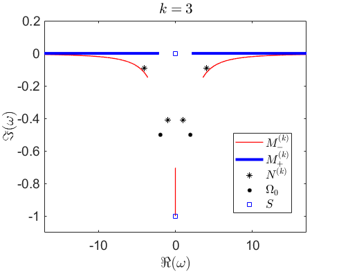
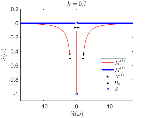
Figure 1: The sets $M^{(k)}_{+},M^{(k)}_{-},N^{(k)}$, $\Omega_{0}$, and $S$ for the setting in (2.27) and (2.28) with $k=3$ and $k=0.7$.

Finally, for the set $N^{(k)}$ we get by a simple calculation

$$N^{(k)}=\left\{\omega\in D(\tilde{W}):\omega^{4}+{\rm i}\gamma\omega^{3}-\left(2\pi\omega_{p}^{2}+k^{2}\frac{2+\eta}{1+\eta}\right)\omega^{2}-{\rm i}\gamma k^{2}\frac{2+\eta}{1+\eta}\omega+\frac{2\pi\omega_{p}^{2}k^{2}}{1+\eta}=0\right\}\setminus(\Omega_{0}\cup M^{(k)}_{+}\cup M^{(k)}_{-}),$$

which shows that $N^{(k)}$ consists of at most four points in $\mathbb{C}$.

2.2 Main Results in Two Dimensions

For the two-dimensional setting we define the operator pencil

$${\mathcal{P}}:={\mathcal{L}}:=(L(\omega;\lambda))_{\begin{subarray}{c}\omega\in D(\tilde{W})\\ \lambda\in\mathbb{C}\end{subarray}},$$

where

$$L(\omega;\lambda):=A(\omega)-\lambda B(\omega),\ A(\omega)u:=\nabla\times\nabla\times u,\ B(\omega)u:=W(x_{1},\omega)u,\ \nabla:=(\partial_{x_{1}},\partial_{x_{2}},0)^{T}.$$

Just like in the one-dimensional case, we also define

$$L(\omega):=L(\omega;1).$$

Next, we describe our choice of function spaces. This choice is motivated in Sec. 4. We set

$$H:=L^{2}(\mathbb{R}^{2},\mathbb{C}^{3})$$

and choose the domain

$${\mathcal{D}}_{\omega}:=\{E\in L^{2}(\mathbb{R}^{2},\mathbb{C}^{3}):\nabla\times E,\nabla\times\nabla\times E\in L^{2}(\mathbb{R}^{2},\mathbb{C}^{3}),\nabla\cdot(\tilde{W}E)=0\ (\text{distributionally})\}.$$ (2.29)

The range space becomes

$${\mathcal{R}}:=\{r\in L^{2}(\mathbb{R}^{2},\mathbb{C}^{3}):\nabla\cdot r=0\ \text{distributionally}\}$$ (2.30)

equipped with the $L^{2}$-inner product.

Analogously to the 1D case $B(\omega):H\supset{\mathcal{D}}_{\omega}\to{\mathcal{R}}$ is bounded and $A(\omega):H\supset{\mathcal{D}}_{\omega}\to{\mathcal{R}}$ is closed since it is bounded as an operator from ${\mathcal{D}}_{\omega}$ to ${\mathcal{R}}$. Also here the Hilbert space property of ${\mathcal{D}}_{\omega}$ is used, see Lemma 4.1.

Using the notation

$$M_{\pm}:= \{\omega\in D(\tilde{W})\setminus\Omega_{0}:W_{\pm}(\omega)\in(0,\infty)\},$$ (2.31)

$$N:= \{\omega\in D(\tilde{W})\setminus\Omega_{0}:\text{ there exists }a\geq 0\text{ such that }W_{\pm}(\omega)\notin[a,\infty)\text{ and }\eqref{E:ev.cond-2D}\text{ holds}\},$$ (2.32)

$$a(W_{+}(\omega)+W_{-}(\omega))=W_{+}(\omega)W_{-}(\omega),$$ (2.33)

and an analogous notation to (2.6) for the ”reduced” spectrum outside $\Omega_{0}$, our main results are

Theorem 3 (Two dimensions; reduced spectrum).

Spectrum:

$$\sigma^{{\rm red}}({\mathcal{L}})=M_{+}\cup M_{-}\cup N.$$ (2.34)

Point spectrum:

$$\sigma_{p}^{{\rm red}}({\mathcal{L}})=\emptyset.$$ (2.35)

Essential and Weyl spectrum:

$$\sigma^{{\rm red}}_{e,j}({\mathcal{L}})=\sigma_{\text{Weyl}}^{{\rm red}}({\mathcal{L}})=M_{+}\cup M_{-}\cup N,\ j=1,\dots,5.$$ (2.36)

Theorem 4 (Two dimensions; exceptional set).

Spectrum:

$$\sigma({\mathcal{L}})\cap\Omega_{0}=\Omega_{0}.$$ (2.37)

Point spectrum:

$$\sigma_{p}^{(<\infty)}({\mathcal{L}})\cap\Omega_{0} =\leavevmode\nobreak\ \emptyset,$$ (2.38)

$$\sigma_{p}^{(\infty)}({\mathcal{L}})\cap\Omega_{0} =\leavevmode\nobreak\ \{\omega\in\Omega_{0}:\tilde{W}_{+}(\omega)=0\text{ or }\tilde{W}_{-}(\omega)=0\text{ or }\tilde{W}_{+}(\omega)+\tilde{W}_{-}(\omega)=0\}.$$

Essential and Weyl spectrum:

$$\sigma_{e,j}({\mathcal{L}})\cap\Omega_{0}=\sigma_{\text{Weyl}}({\mathcal{L}})\cap\Omega_{0}=\Omega_{0},\ j=1,\dots,5.$$ (2.39)

Remark 2.6 (Block diagonal structure).

Just like in the 1D case the operator at hand has a block diagonal structure as visible in (1.10) and (4.2). As a result, the spectrum of ${\mathcal{L}}$ is the union of the spectra of ${\mathcal{L}}^{(1,2)}$ and ${\mathcal{L}}^{(3)}$ in the sense of $\eqref{E:Pspec}$, where

$${\mathcal{L}}^{(1,2)}:=\left(\begin{smallmatrix}-\partial_{x_{2}}^{2}&\partial_{x_{1}}\partial_{x_{2}}\\ \partial_{x_{1}}\partial_{x_{2}}&-\partial_{x_{1}}^{2}\end{smallmatrix}\right)-\lambda W(x_{1},\omega)$$

and ${\mathcal{L}}^{(3)}:=-\partial_{x_{1}}^{2}-\partial_{x_{2}}^{2}-\lambda W(x_{1},\omega)$ with the domains

$$D({\mathcal{L}}^{(1,2)}) :=\{(u_{1},u_{2})^{T}:u\in{\mathcal{D}}_{\omega}\},$$

$$D({\mathcal{L}}^{(3)}) :=\{u_{3}:u\in{\mathcal{D}}_{\omega}\}.$$

Example 2.7.

In Fig. 2 we plot the sets $M_{+},M_{-},N$, $\Omega_{0}$, and $S$ for the same interface studied in Example 2.5, i.e. with $\tilde{W}$ given by (2.27) and (1.1) and with the parameters $\eta=1,\gamma=2$, and $\omega_{p}$ specified below. The sets $\Omega_{0}$ and $S$ are the same as in Example 2.5 and $M_{+}=\mathbb{R}\setminus\{0\}$. For $M_{-}$ we get

$$M_{-}=M^{(0)}=\cup_{k>0}M_{-}^{(k)}$$

with $M_{-}^{(k)}$ from Example 2.5. Hence, for $\omega\in M^{(k)}_{-}\cap{\rm i}\mathbb{R}$, $\Im(\omega)$ is still bounded below by $-\gamma$.

In Fig. 2 we study three values of the parameter $\omega_{p}$: $1,0.701,$ and $0.6$. The set $N$ consists of three components. The union of the two unbounded components united with $\Omega_{0}$ is closed in $\mathbb{C}$: for $a\to\infty$ the corresponding solution of (2.33) satisfies $\omega\to\infty$ or $\omega\to-\infty$ and for $a\to 0+$ we have $\omega\to\omega_{0}\in\Omega_{0}$. On the other hand, the bounded component of $N$ is not closed. For $a\to\infty$ the corresponding solution $\omega(a)$ of (2.33) converges to a zero of $\tilde{W}_{+}+\tilde{W}_{-}$, i.e. to one of the points $\omega_{*}^{\pm}:=\frac{1}{2}\left(-{\rm i}\gamma\pm\sqrt{8\pi\omega_{p}^{2}/(\eta+2)-\gamma^{2}}\right)$, in such a way that $a(W_{+}(\omega(a))+W_{-}(\omega(a)))\to W_{+}(\omega_{*}^{\pm})W_{-}(\omega_{*}^{\pm})$ as $a\to\infty$. The points $\omega_{*}^{\pm}$ are marked by green circles in Fig. 2. As a result, the spectrum of ${\mathcal{L}}$ is not closed in the $\omega$-plane, similarly to the 1D case in Example 2.5. For $\omega_{p}^{2}\leq\gamma^{2}(\eta+2)/(8\pi)$ the points $\omega_{*}^{\pm}$ lie on the imaginary axis and they coincide when $\omega_{p}^{2}=\gamma^{2}(\eta+2)/(8\pi)$. The case $(\omega_{p},\gamma)=(0.701,2)$ corresponds to $\gamma$ slightly above this threshold. Below the threshold the bounded part of $N$ includes a closed curve and a segment on the imaginary axis, which connects $\omega_{*}^{-}$ and $\omega_{*}^{+}$. The last parameter value $\omega_{p}=0.6$ depicted in Fig. 2 is such a case.

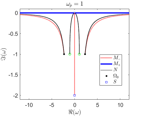
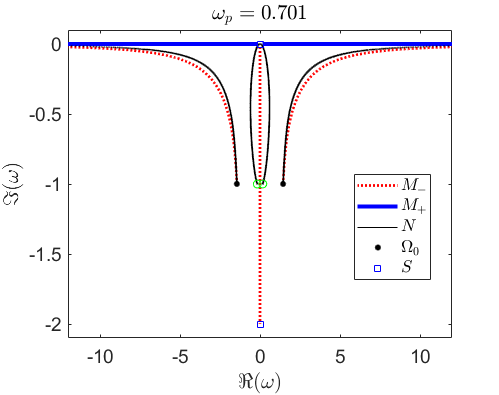
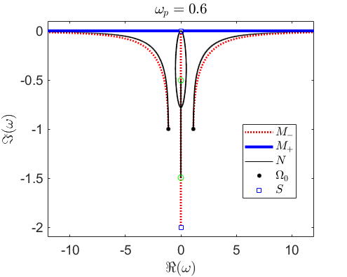
Figure 2: The sets $M_{+},M_{-},N$, $\Omega_{0}$, and $S$ for the 2D setting with the function $\tilde{W}$ as in (2.27), where $(\eta,\gamma)=(1,2)$ and $\omega_{p}\in\{1,0.701,0.6\}$. The green circles mark zeros of $\tilde{W}_{+}+\tilde{W}_{-}$.

3 One-Dimensional Reduction

In this section we study the problem defined in (1.5) and (1.6). The rigorous functional analytic setting is given in Sec. 2.1.

3.1 Explanation of the Functional Analytic Setting

We first note that we have

$$\nabla_{k}\cdot(\tilde{W}u)=(\tilde{W}u_{1})^{\prime}+{\rm i}k\tilde{W}u_{2},$$ (3.1)

$$\nabla_{k}\times u=\left(\begin{smallmatrix}{\rm i}ku_{3}\\ -u_{3}^{\prime}\\ u_{2}^{\prime}-{\rm i}ku_{1}\end{smallmatrix}\right)\quad\text{and}\quad\nabla_{k}\times\nabla_{k}\times u=\left(\begin{smallmatrix}k^{2}u_{1}+{\rm i}ku_{2}^{\prime}\\ {\rm i}ku_{1}^{\prime}-u_{2}^{\prime\prime}\\ -u_{3}^{\prime\prime}+k^{2}u_{3}\end{smallmatrix}\right).$$ (3.2)

We are now able to rewrite ${\mathcal{D}}_{k,\omega}$ in several ways. For $u\in{\mathcal{D}}_{k,\omega}$, we have $u,\nabla_{k}\times u,\nabla_{k}\times\nabla_{k}\times u\in L^{2}(\mathbb{R},\mathbb{C}^{3})$. From (3.2), we see that this is equivalent to the conditions $u_{3}\in H^{2}(\mathbb{R},\mathbb{C})$, $u_{2}\in H^{1}(\mathbb{R},\mathbb{C})$ and $u_{2}^{\prime}-{\rm i}ku_{1}\in H^{1}(\mathbb{R},\mathbb{C})$. Moreover, from (3.1) we see that the divergence condition is satisfied precisely when $\tilde{W}u_{1}\in H^{1}(\mathbb{R},\mathbb{C})$ and $(\tilde{W}u_{1})^{\prime}+{\rm i}k\tilde{W}u_{2}=0$. Therefore, we obtain

$${\mathcal{D}}_{k,\omega}=\{u\in L^{2}(\mathbb{R},\mathbb{C}^{3}):u_{3}\in H^{2}(\mathbb{R},\mathbb{C}),u_{2},u_{2}^{\prime}-{\rm i}ku_{1},\tilde{W}u_{1}\in H^{1}(\mathbb{R},\mathbb{C})\text{ and }(\tilde{W}u_{1})^{\prime}+{\rm i}k\tilde{W}u_{2}=0\}.$$ (3.3)

Next, we reformulate the conditions for lying in $H^{1}(\mathbb{R},\mathbb{C})$ in terms of functions not having a jump across the interface at $x=0$ in the sense of (1.4). This shows that

$${\mathcal{D}}_{k,\omega}= \{u\in L^{2}(\mathbb{R},\mathbb{C}^{3}):\ \nabla_{k}\times u_{\pm},\nabla_{k}\times\nabla_{k}\times u_{\pm}\in L^{2}(\mathbb{R}_{\pm},\mathbb{C}^{3}),$$ (3.4)

$$\quad\text{the divergence condition}\ \eqref{E:div-cond-1d},\ \text{and the interface conditions}\ \eqref{E:IFC-1D}\ \text{hold}\},$$

$$\tilde{W}_{\pm}(\omega)\nabla_{k}\cdot u_{\pm}=\tilde{W}_{\pm}(\omega)(u^{\prime}_{\pm,1}+{\rm i}ku_{\pm,2}) =0\text{ on }\mathbb{R}_{\pm},$$ (3.5)

$$\llbracket\tilde{W}(\omega)u_{1}\rrbracket=\llbracket u_{2}\rrbracket=\llbracket u_{3}\rrbracket=\llbracket u_{2}^{\prime}-{\rm i}ku_{1}\rrbracket=\llbracket u_{3}^{\prime}\rrbracket =0,$$ (3.6)

where we define

$$u_{\pm}:=u|_{\mathbb{R}_{\pm}},\text{ with }\mathbb{R}_{\pm}:=\{x\in\mathbb{R}:\pm x>0\}.$$

For a detailed proof, see Lemma B.1 in Appendix B.

Also,

$${\mathcal{D}}_{k,\omega}=\{u\in L^{2}(\mathbb{R},\mathbb{C}^{3}):u_{\pm,3}\in H^{2}(\mathbb{R}_{\pm},\mathbb{C}),u_{\pm,2},u_{\pm,2}^{\prime}-{\rm i}ku_{\pm,1},\tilde{W}_{\pm}u_{\pm,1}\in H^{1}(\mathbb{R}_{\pm},\mathbb{C})\text{ and }\eqref{E:div-cond-1d},\eqref{E:IFC-1D}\text{ hold}\},$$

which follows just like in (3.3).

Note that using the range space ${\mathcal{R}}_{k}$ (which is a closed subspace of $L^{2}(\mathbb{R},\mathbb{C}^{3})$), see (2.2), instead of $L^{2}(\mathbb{R},\mathbb{C}^{3})$ is necessary for the spectral analysis. Namely, when investigating the resolvent set of the spectral problem, we have to consider the inhomogeneous problem

$$T_{k}(\partial_{x_{1}})u-W(\omega)u=r,$$ (3.7)

where $r\in L^{2}(\mathbb{R},\mathbb{C}^{3})$. Since, for $u\in{\mathcal{D}}_{k,\omega}$ the left hand side of (3.7) is divergence free, we have to impose the condition $\nabla_{k}\cdot r=0$ (in the distributional sense) also to the right hand side of (3.7); otherwise, the resolvent set would be empty, implying that the spectrum would be the whole of $D(\tilde{W})$.

The functional setting is non-standard as the domain of the pencil is not contained within its range space. Indeed, unless $W_{+}=W_{-}$, there exist $u\in{\mathcal{D}}_{k,\omega}$ such that $\nabla_{k}\cdot u\neq 0$, which can be concluded using only the interface conditions. The functions $u\in{\mathcal{D}}_{k,\omega}$ satisfy $\llbracket\tilde{W}u_{1}\rrbracket=0$ and hence $u_{1}$ is discontinuous unless $W_{+}=W_{-}$, while the functions $f\in{\mathcal{R}}_{k}$ satisfy $\nabla_{k}\cdot f=0$. Thus $f_{1}^{\prime}=-{\rm i}kf_{2}\in L^{2}(\mathbb{R})$, i.e. $f_{1}\in H^{1}(\mathbb{R})$ and $f_{1}$ is continuous. In summary ${\mathcal{D}}_{k,\omega}\not\subset{\mathcal{R}}_{k}$.

We equip ${\mathcal{D}}_{k,\omega}$ with the inner product

$$\langle u,v\rangle_{{\mathcal{D}}_{k,\omega}}:=\langle u,v\rangle_{L^{2}}+\langle\nabla_{k}\times\nabla_{k}\times u,\nabla_{k}\times\nabla_{k}\times v\rangle_{L^{2}},u,v\in{\mathcal{D}}_{k,\omega},$$ (3.8)

which corresponds to the graph norm (1.13) in our abstract setting. As we show next, ${\mathcal{D}}_{k,\omega}$ equipped with this inner product is a Hilbert space. (Note that, equivalently, we could show that $A(\omega):{\mathcal{D}}_{k,\omega}\to{\mathcal{R}}$ is closed.)

Lemma 3.1.

$({\mathcal{D}}_{k,\omega},\langle\cdot,\cdot\rangle_{{\mathcal{D}}_{k,\omega}})$ is a Hilbert space for any $k\in\mathbb{R}$ and $\omega\in D(\tilde{W})$.

Proof.

First note that the norm

$$\|v\|:=\left(\|v\|_{L^{2}(\mathbb{R})}^{2}+\|\nabla_{k}\times v\|_{L^{2}(\mathbb{R})}^{2}+\|\nabla_{k}\times\nabla_{k}\times v\|_{L^{2}(\mathbb{R})}^{2}\right)^{1/2}$$

is equivalent to the norm generated by $\langle\cdot,\cdot\rangle_{{\mathcal{D}}_{k,\omega}}$ as (via Lemma A.1)

$$\|\nabla_{k}\times v\|_{L^{2}(\mathbb{R})}^{2}=\langle v,\nabla_{k}\times\nabla_{k}\times v\rangle_{L^{2}}\leq\|v\|_{L^{2}(\mathbb{R})}\|\nabla_{k}\times\nabla_{k}\times v\|_{L^{2}(\mathbb{R})}$$

for each $v\in{\mathcal{D}}_{k,\omega}$. Here, for the application of Lemma A.1 we set $u:=\nabla_{k}\times v$. Due to $v\in{\mathcal{D}}_{k,\omega}$ we know that $u,\nabla_{k}\times u\in L^{2}$ and hence the assumptions of the lemma are indeed satisfied.

Let $(u_{n})\subset{\mathcal{D}}_{k,\omega}$ be a Cauchy sequence. Due to the above norm equivalence we have that $(u_{n}),(\nabla_{k}\times u_{n})$, and $(\nabla_{k}\times\nabla_{k}\times u_{n})$ are Cauchy in $L^{2}(\mathbb{R},\mathbb{C}^{3})$. Hence there are $u,f,g\in L^{2}(\mathbb{R},\mathbb{C}^{3})$ such that

$$u_{n}\to u,\nabla_{k}\times u_{n}\to f,\ \text{and}\ \nabla_{k}\times\nabla_{k}\times u_{n}\to g\quad\text{in}\quad L^{2}(\mathbb{R},\mathbb{C}^{3}).$$ (3.9)

Because

$$\int_{\mathbb{R}}u\cdot(\nabla_{k}\times\phi)\,{\rm d}x=\lim_{n\to\infty}\int_{\mathbb{R}}u_{n}\cdot(\nabla_{k}\times\phi)\,{\rm d}x=\lim_{n\to\infty}\int_{\mathbb{R}}(\nabla_{k}\times u_{n})\cdot\phi\,{\rm d}x=\int_{\mathbb{R}}f\cdot\phi\,{\rm d}x$$

for each $\phi\in C^{\infty}_{c}(\mathbb{R},\mathbb{C}^{3})$, we get $\nabla_{k}\times u=f$. Analogously, we obtain $\nabla_{k}\times\nabla_{k}\times u=g$.

Since

$$\int_{\mathbb{R}}(\tilde{W}u)\cdot\nabla_{k}\varphi\,{\rm d}x=\lim_{n\to\infty}\int_{\mathbb{R}}(\tilde{W}u_{n})\cdot\nabla_{k}\varphi\,{\rm d}x=0$$

for each $\varphi\in C^{\infty}_{c}(\mathbb{R},\mathbb{C})$, we have $\nabla_{k}\cdot(\tilde{W}u)=0$. We conclude that $u\in{\mathcal{D}}_{k,\omega}$ and due to (3.9) we have also $u_{n}\to u$ in ${\mathcal{D}}_{k,\omega}$. ∎

3.2 A Subset of the Resolvent Set $\rho^{{\rm red}}({\mathcal{L}}_{k})$

First, we restrict our attention to the set $\omega\in D(\tilde{W})\setminus\Omega_{0}$. Note that for $\omega\in D(\tilde{W})\setminus\Omega_{0}$ the divergence condition (3.5) reduces to

$$\nabla_{k}\cdot u_{\pm}=0\text{ on }\mathbb{R}_{\pm}.$$ (3.10)

The first step towards the proof of Theorem 1 is the following

Proposition 3.2.

$$\sigma^{{\rm red}}({\mathcal{L}}_{k})\subset(M^{(k)}_{+}\cup M^{(k)}_{-})\dot{\cup}N^{(k)}=:{\mathcal{M}}^{(k)},$$

where $M^{(k)}_{\pm}$ and $N^{(k)}$ are defined in (2.4) and (2.5).

Remark 3.3.

In other words, the proposition states that for the resolvent set we have

$$\rho^{{\rm red}}({\mathcal{L}}_{k})\supset D(\tilde{W})\setminus(\Omega_{0}\cup{\mathcal{M}}^{(k)}).$$

Remark 3.4.

In several of the subsequent calculations, we will make use of the following equivalent descriptions of $N^{(k)}$.

$$N^{(k)}= \leavevmode\nobreak\ \{\omega\in D(\tilde{W})\setminus\Omega_{0}:W_{+}(\omega),W_{-}(\omega)\notin[k^{2},\infty),\tilde{W}_{+}(\omega)\sqrt{k^{2}-W_{-}(\omega)}+\tilde{W}_{-}(\omega)\sqrt{k^{2}-W_{+}(\omega)}=0\}$$

$$= \leavevmode\nobreak\ \{\omega\in D(\tilde{W})\setminus\Omega_{0}:W_{+}(\omega),W_{-}(\omega)\notin[k^{2},\infty),W_{+}(\omega)\sqrt{k^{2}-W_{-}(\omega)}+W_{-}(\omega)\sqrt{k^{2}-W_{+}(\omega)}=0\}.$$

The second equality follows because the condition $\omega\in D(\tilde{W})\setminus\Omega_{0}$ excludes $\omega=0$. Indeed, if $0\notin\Omega_{0}$, then necessarily $\tilde{W}$ has a singularity at $\omega=0$, implying $0\notin D(\tilde{W})$.
For the first equality we show that, for $\omega\in D(\tilde{W})\setminus\Omega_{0}$ such that $W_{+}(\omega),W_{-}(\omega)\notin[k^{2},\infty)$, equation (2.3) and

$$W_{+}(\omega)\sqrt{k^{2}-W_{-}(\omega)}=-W_{-}(\omega)\sqrt{k^{2}-W_{+}(\omega)}$$ (3.11)

are equivalent.
Clearly (2.3) follows from (3.11) by squaring and using $W_{+}(\omega)\neq W_{-}(\omega)$ which is also a consequence of (3.11). Assume now (2.3). Then we get $(k^{2}-W_{+}(\omega))(k^{2}-W_{-}(\omega))=k^{4}$ and thus

$$\sqrt{k^{2}-W_{-}(\omega)}=\sqrt{\frac{k^{4}}{k^{2}-W_{+}(\omega)}}=k^{2}\sqrt{\frac{1}{k^{2}-W_{+}(\omega)}}=k^{2}\frac{1}{\sqrt{k^{2}-W_{+}(\omega)}}$$ (3.12)

as $k^{2}-W_{+}(\omega)\notin(-\infty,0]$. At the same time (2.3) implies $W_{-}(\omega)(k^{2}-W_{+}(\omega))=-k^{2}W_{+}(\omega)$ and hence

$$W_{-}(\omega)=-k^{2}\frac{W_{+}(\omega)}{k^{2}-W_{+}(\omega)}.$$ (3.13)

Using (3.12) and (3.13), we obtain

$$W_{+}(\omega)\sqrt{k^{2}-W_{-}(\omega)}+W_{-}(\omega)\sqrt{k^{2}-W_{+}(\omega)}=k^{2}\frac{W_{+}(\omega)}{\sqrt{k^{2}-W_{+}(\omega)}}-k^{2}\frac{W_{+}(\omega)}{k^{2}-W_{+}(\omega)}\sqrt{k^{2}-W_{+}(\omega)}=0,$$

showing the desired equality of the sets.

Proof.

(of Prop. 3.2) Let $r\in{\mathcal{R}}_{k}$ and $\omega\in D(\tilde{W})\setminus(\Omega_{0}\cup{\mathcal{M}}^{(k)})$. We need to show the existence of a unique $u\in{\mathcal{D}}_{k,\omega}$ such that

$$\left.\begin{array}[]{rcl}(k^{2}-W(\omega))u_{1}+{\rm i}ku_{2}^{\prime}&=&r_{1}\\ {\rm i}ku_{1}^{\prime}-u_{2}^{\prime\prime}-W(\omega)u_{2}&=&r_{2}\\ -u_{3}^{\prime\prime}+(k^{2}-W(\omega))u_{3}&=&r_{3}\end{array}\right\}{\rm\leavevmode\nobreak\ on\leavevmode\nobreak\ }(-\infty,0){\rm\leavevmode\nobreak\ and\leavevmode\nobreak\ }(0,\infty).$$ (3.14)

We solve the first equation for $u_{1}$:

$$u_{1}=\dfrac{r_{1}-{\rm i}ku_{2}^{\prime}}{k^{2}-W(\omega)}.$$ (3.15)

By (3.10), we have $r_{1}^{\prime}=-{\rm i}kr_{2}$ and hence, by (3.15)

$$u_{1}^{\prime}=-\dfrac{{\rm i}k}{k^{2}-W(\omega)}(u^{\prime\prime}_{2}+r_{2})\ \text{ on }(-\infty,0)\text{ and }(0,\infty).$$ (3.16)

Transferring this into the second equation in (3.14) gives

$$\dfrac{k^{2}}{k^{2}-W(\omega)}(u^{\prime\prime}_{2}+r_{2})-u^{\prime\prime}_{2}-W(\omega)u_{2}=r_{2},$$

and using $W\neq 0$,

$$-u^{\prime\prime}_{2}+(k^{2}-W(\omega))u_{2}=r_{2}\quad\mbox{ on }(-\infty,0)\mbox{ and }(0,\infty).$$ (3.17)

Next, we apply the variation of parameters formula to (3.17) and search for an $L^{2}(\mathbb{R})$-solution $u_{2}$ with $\llbracket u_{2}\rrbracket=0$. We need the following lemma.

Lemma 3.5.

Let $\mu\in\mathbb{C},\Re\mu>0,r\in L^{2}(\mathbb{R})$. Then

$$\psi_{1}(x) :=e^{\mu x}\int_{x}^{\infty}e^{-\mu t}r(t)\,{\rm d}t\text{ satisfies }\psi_{1}\in L^{2}(0,\infty)\mbox{ with }\left\|\psi_{1}\right\|_{L^{2}(0,\infty)}\leq\dfrac{1}{\Re\mu}\left\|r\right\|_{L^{2}},$$ (3.18)

$$\psi_{2}(x) :=e^{-\mu x}\int_{0}^{x}e^{\mu t}r(t)\,{\rm d}t\text{ satisfies }\psi_{2}\in L^{2}(0,\infty)\mbox{ with }\left\|\psi_{2}\right\|_{L^{2}(0,\infty)}\leq\dfrac{1}{\Re\mu}\left\|r\right\|_{L^{2}}.$$ (3.19)

Proof.

Let us prove (3.18) in detail; (3.19) can be shown similarly. Choose $x_{0}>0$ and set $\alpha:=\Re\mu$. Then

$$\|\psi_{1}\|_{L^{2}(0,x_{0})}^{2}\leq\int_{0}^{x_{0}}e^{2\alpha x}\left(\int_{x}^{\infty}e^{-\alpha t}|r(t)|\,{\rm d}t\right)^{2}\,{\rm d}x$$

$$=\left.\dfrac{1}{2\alpha}e^{2\alpha x}\left(\int_{x}^{\infty}e^{-\alpha t}|r(t)|\,{\rm d}t\right)^{2}\right|_{0}^{x_{0}}+\dfrac{1}{\alpha}\underbrace{\int_{0}^{x_{0}}e^{\alpha x}|r(x)|\left(\int_{x}^{\infty}e^{-\alpha t}|r(t)|\,{\rm d}t\right)\,{\rm d}x}_{=:I(x_{0})}.$$

Next we estimate $I(x_{0})$.

$$I(x_{0}) \leq\sqrt{\int_{0}^{x_{0}}e^{2\alpha x}\left(\int_{x}^{\infty}e^{-\alpha t}|r(t)|\,{\rm d}t\right)^{2}\,{\rm d}x}\sqrt{\int_{0}^{x_{0}}|r(x)|^{2}\,{\rm d}x}$$

$$\leq\lambda\int_{0}^{x_{0}}e^{2\alpha x}\left(\int_{x}^{\infty}e^{-\alpha t}|r(t)|\,{\rm d}t\right)^{2}\,{\rm d}x+\dfrac{1}{4\lambda}\int_{0}^{x_{0}}|r(x)|^{2}\,{\rm d}x$$

for any $\lambda>0$. Choosing $\lambda\in(0,\alpha)$ yields

$$\|\psi_{1}\|_{L^{2}(0,x_{0})}^{2} \leq\frac{1}{1-\dfrac{\lambda}{\alpha}}\left[\dfrac{1}{2\alpha}e^{2\alpha x}\left.\left(\int_{x}^{\infty}e^{-\alpha t}|r(t)|\,{\rm d}t\right)^{2}\right|_{0}^{x_{0}}+\dfrac{1}{4\alpha\lambda}\int_{0}^{x_{0}}|r(x)|^{2}\,{\rm d}x\right]$$

$$\leq\frac{\alpha}{\alpha-\lambda}\left[\dfrac{1}{2\alpha}e^{2\alpha x_{0}}\left(\int_{x_{0}}^{\infty}e^{-\alpha t}|r(t)|\,{\rm d}t\right)^{2}+\dfrac{1}{4\alpha\lambda}\int_{0}^{x_{0}}|r(x)|^{2}\,{\rm d}x\right]$$

$$\leq\frac{\alpha}{\alpha-\lambda}\left[\dfrac{1}{4\alpha^{2}}\int_{x_{0}}^{\infty}|r(t)|^{2}\,{\rm d}t+\dfrac{1}{4\alpha\lambda}\int_{0}^{x_{0}}|r(x)|^{2}\,{\rm d}x\right]$$

$$\leq\dfrac{1}{4\alpha(\alpha-\lambda)}\int_{x_{0}}^{\infty}|r(t)|^{2}\,{\rm d}t+\dfrac{1}{4\lambda(\alpha-\lambda)}\int_{0}^{x_{0}}|r(t)|^{2}\,{\rm d}t,$$

where the third step follows by integration by parts. Now setting $\lambda=\alpha/2$ and letting $x_{0}\to\infty$, we obtain (3.18). ∎

Below we use the notation

$$\mu_{\pm}:=\sqrt{k^{2}-W_{\pm}},$$

where the $\omega$ dependence of $W_{\pm}$ and $\mu_{\pm}$ has been suppressed. Note that $\Re\mu_{\pm}>0$ because $\omega\notin M^{(k)}_{\pm}$. The variation of parameters formula applied to (3.17) together with the $L^{2}-$condition for $u_{2}$ in (2.1) and the second interface condition $\llbracket u_{2}\rrbracket=0$ in (3.6) yield

$$u_{2}(x_{1}) =\left[C_{2}(k)-\dfrac{1}{2\mu_{+}}\int_{0}^{\infty}e^{-\mu_{+}t}r_{2}(t)\,{\rm d}t\right]e^{-\mu_{+}x_{1}}$$ (3.20)

$$+\dfrac{1}{2\mu_{+}}\left[e^{\mu_{+}x_{1}}\int_{x_{1}}^{\infty}e^{-\mu_{+}t}r_{2}(t)\,{\rm d}t+e^{-\mu_{+}x_{1}}\int_{0}^{x_{1}}e^{\mu_{+}t}r_{2}(t)\,{\rm d}t\right]\mbox{ for }x_{1}\in(0,\infty),$$

$$u_{2}(x_{1}) =\left[C_{2}(k)-\dfrac{1}{2\mu_{-}}\int_{-\infty}^{0}e^{\mu_{-}t}r_{2}(t)\,{\rm d}t\right]e^{\mu_{-}x_{1}}$$ (3.21)

$$+\dfrac{1}{2\mu_{-}}\left[e^{\mu_{-}x_{1}}\int_{x_{1}}^{0}e^{-\mu_{-}t}r_{2}(t)\,{\rm d}t+e^{-\mu_{-}x_{1}}\int_{-\infty}^{x_{1}}e^{\mu_{-}t}r_{2}(t)\,{\rm d}t\right]\mbox{ for }x_{1}\in(-\infty,0),$$

with $C_{2}(k)\in\mathbb{C}$ denoting a free constant. We track the $k-$dependence of the constants for the purposes of the two-dimensional case in Sec. 4. Now (3.15) gives

$$u_{1}(x_{1})=\dfrac{1}{\mu_{+}^{2}}\Big{\{}r_{1}(x_{1})+{\rm i}k\mu_{+}\Big{[}C_{2}(k)-\dfrac{1}{2\mu_{+}}\int_{0}^{\infty}e^{-\mu_{+}t}r_{2}(t)\,{\rm d}t\Big{]}e^{-\mu_{+}x_{1}}$$

$$-\dfrac{1}{2}{\rm i}k\Big{[}e^{\mu_{+}x_{1}}\int_{x_{1}}^{\infty}e^{-\mu_{+}t}r_{2}(t)\,{\rm d}t-e^{-\mu_{+}x_{1}}\int_{0}^{x_{1}}e^{\mu_{+}t}r_{2}(t)\,{\rm d}t\Big{]}\Big{\}}\quad\mbox{ for }x_{1}\in(0,\infty),$$ (3.22)

$$u_{1}(x_{1})=\frac{1}{\mu_{-}^{2}}\Big{\{}r_{1}(x_{1})-{\rm i}k\mu_{-}\Big{[}C_{2}(k)-\dfrac{1}{2\mu_{-}}\int_{-\infty}^{0}e^{\mu_{-}t}r_{2}(t)\,{\rm d}t\Big{]}e^{\mu_{-}x_{1}}$$

$$-\dfrac{1}{2}{\rm i}k\Big{[}e^{\mu_{-}x_{1}}\int_{x_{1}}^{0}e^{-\mu_{-}t}r_{2}(t)\,{\rm d}t-e^{-\mu_{-}x_{1}}\int_{-\infty}^{x_{1}}e^{\mu_{-}t}r_{2}(t)\,{\rm d}t\Big{]}\Big{\}}\quad\mbox{ for }x_{1}\in(-\infty,0).$$ (3.23)

Next, we ensure that the first interface condition in (3.6) is satisfied. Note that $r\in{\mathcal{R}}_{k}$ implies $r_{1}\in H^{1}(\mathbb{R})$ and hence $r_{1}$ is continuous. Equations (3.22) and (3.23) imply that

$$u_{1}(0+)=\dfrac{1}{\mu_{+}}{\rm i}kC_{2}(k)+\dfrac{1}{\mu_{+}^{2}}\Big{[}r_{1}(0)-{\rm i}k\int_{0}^{\infty}e^{-\mu_{+}t}r_{2}(t)\,{\rm d}t\Big{]},$$ (3.24)

$$u_{1}(0-)=-\dfrac{1}{\mu_{-}}{\rm i}kC_{2}(k)+\dfrac{1}{\mu_{-}^{2}}\Big{[}r_{1}(0)+{\rm i}k\int_{-\infty}^{0}e^{\mu_{-}t}r_{2}(t)\,{\rm d}t\Big{]}.$$

Noting that $\frac{\tilde{W}_{+}}{\mu_{+}}+\frac{\tilde{W}_{-}}{\mu_{-}}=\frac{1}{\mu_{+}\mu_{-}}\Big{[}\tilde{W}_{+}\mu_{-}+\tilde{W}_{-}\mu_{+}\Big{]}\neq 0$ by the assumption $\omega\notin N^{(k)}$ (see Remark 3.4), the first interface condition in (3.6) gives

$$C_{2}(k)=\dfrac{1}{\frac{\tilde{W}_{+}}{\mu_{+}}+\frac{\tilde{W}_{-}}{\mu_{-}}}\Big{[}\underbrace{\Big{(}\dfrac{\tilde{W}_{-}}{\mu_{-}^{2}}-\dfrac{\tilde{W}_{+}}{\mu_{+}^{2}}\Big{)}}_{=\frac{1}{\mu_{+}^{2}\mu_{-}^{2}}k^{2}(\tilde{W}_{-}-\tilde{W}_{+})}\frac{r_{1}(0)}{{\rm i}k}+\dfrac{\tilde{W}_{+}}{\mu_{+}^{2}}\int_{0}^{\infty}e^{-\mu_{+}t}r_{2}(t)\,{\rm d}t+\dfrac{\tilde{W}_{-}}{\mu_{-}^{2}}\int_{-\infty}^{0}e^{\mu_{-}t}r_{2}(t)\,{\rm d}t\Big{]}$$

$$=\dfrac{1}{\mu_{+}\mu_{-}(\tilde{W}_{+}\mu_{-}+\tilde{W}_{-}\mu_{+})}\Big{[}{\rm i}k(\tilde{W}_{+}-\tilde{W}_{-})r_{1}(0)+\tilde{W}_{+}\mu_{-}^{2}\int_{0}^{\infty}e^{-\mu_{+}t}r_{2}(t)\,{\rm d}t+\tilde{W}_{-}\mu_{+}^{2}\int_{-\infty}^{0}e^{\mu_{-}t}r_{2}(t)\,{\rm d}t\Big{]}$$ (3.25)

provided $k\neq 0$. If $k=0$, then $C_{2}(k)$ is arbitrary since (3.24) gives $u_{1}(0+)=-r_{1}(0)/W_{+}(\omega)$ and $u_{1}(0-)=-r_{1}(0)/W_{-}(\omega)$, which implies the interface condition.

Finally, the differential equation for $u_{3}$ in (3.14) has the same form as (3.17). Hence, together with the $L^{2}-$condition for $u_{3}$ in (2.1) and the third interface condition $\llbracket u_{3}\rrbracket=0$ in (3.6) we obtain (3.20), (3.21) also for $u_{3}$, with a new constant $C_{3}(k)$ and $r_{3}$ instead of $r_{2}$ on the right-hand side. Next, the interface condition $\llbracket u_{3}^{\prime}\rrbracket=0$ reads

$$-\mu_{+}\Big{[}C_{3}(k)-\dfrac{1}{2\mu_{+}}\int_{0}^{\infty}e^{-\mu_{+}t}r_{3}(t)dt\Big{]}+\dfrac{1}{2}\int_{0}^{\infty}e^{-\mu_{+}t}r_{3}(t)dt$$

$$=\mu_{-}\Big{[}C_{3}(k)-\dfrac{1}{2\mu_{-}}\int_{-\infty}^{0}e^{\mu_{-}t}r_{3}(t)dt\Big{]}-\dfrac{1}{2}\int_{-\infty}^{0}e^{\mu_{-}t}r_{3}(t)dt,$$

which gives, noting that $\mu_{+}+\mu_{-}\neq 0$ since $\Re\mu_{\pm}>0$,

$$C_{3}(k)=\dfrac{1}{\mu_{+}+\mu_{-}}\Big{[}\int_{0}^{\infty}e^{-\mu_{+}t}r_{3}(t)dt+\int_{-\infty}^{0}e^{\mu_{-}t}r_{3}(t)dt\Big{]}.$$ (3.26)

The expressions (3.20), (3.21) (also for $u_{3}$), (3.22), (3.23), (3.2), and (3.26) uniquely determine the function $u\in L^{2}(\mathbb{R},\mathbb{C}^{3})$ which satisfies the differential equations (3.14) and all the interface conditions (3.6) except for $\llbracket u_{2}^{\prime}-{\rm i}ku_{1}\rrbracket=0$. We are left to show that this $u$ also satisfies the divergence condition (3.5), the last interface condition $\llbracket u_{2}^{\prime}-{\rm i}ku_{1}\rrbracket=0$, the $L^{2}$ conditions in (2.1), and the estimate

$$\|u\|_{L^{2}(\mathbb{R})}\leq C\|r\|_{L^{2}(\mathbb{R})}\mbox{ with }C\mbox{ independent of }r.$$ (3.27)

For this purpose, we first note that due to Lemma 3.5, for each $\varphi\in L^{2}(\mathbb{R},\mathbb{C})$ and each $\mu\in\mathbb{C}$ such that $\Re\mu>0$,

$$\left\|e^{\mu\cdot}\int_{\cdot}^{\infty}e^{-\mu t}\varphi(t)\,{\rm d}t\right\|_{L^{2}(0,\infty)},\left\|e^{-\mu\cdot}\int_{0}^{\cdot}e^{\mu t}\varphi(t)\,{\rm d}t\right\|_{L^{2}(0,\infty)}\leq\dfrac{1}{\Re\mu}\left\|\varphi\right\|_{L^{2}(0,\infty)},$$ (3.28)

and also

$$\left\|e^{\mu\cdot}\int_{\cdot}^{0}e^{-\mu t}\varphi(t)\,{\rm d}t\right\|_{L^{2}(-\infty,0)},\left\|e^{-\mu\cdot}\int_{-\infty}^{\cdot}e^{\mu t}\varphi(t)\,{\rm d}t\right\|_{L^{2}(-\infty,0)}\leq\dfrac{1}{\Re\mu}\left\|\varphi\right\|_{L^{2}(-\infty,0)}.$$ (3.29)

Consequently, (3.20), (3.21) show that

$$\left\|u_{2,3}\right\|_{L^{2}(0,\infty)} \leq\dfrac{1}{\sqrt{2\Re\mu_{+}}}\Big{[}|C_{2,3}(k)|+\left(\dfrac{1}{2\Re\mu_{+}}\right)^{3/2}\left\|r_{2,3}\right\|_{L^{2}(0,\infty)}\Big{]}+\dfrac{1}{(\Re\mu_{+})^{2}}\left\|r_{2,3}\right\|_{L^{2}(0,\infty)}$$

$$\leq\dfrac{1}{\sqrt{2\Re\mu_{+}}}|C_{2,3}|(k)+\dfrac{5}{4(\Re\mu_{+})^{2}}\left\|r_{2,3}\right\|_{L^{2}(0,\infty)},$$ (3.30)

$$\left\|u_{2,3}\right\|_{L^{2}(-\infty,0)} \leq\dfrac{1}{\sqrt{2\Re\mu_{-}}}\Big{[}|C_{2,3}(k)|+\left(\dfrac{1}{2\Re\mu_{-}}\right)^{3/2}\left\|r_{2,3}\right\|_{L^{2}(-\infty,0)}\Big{]}+\dfrac{1}{(\Re\mu_{-})^{2}}\left\|r_{2,3}\right\|_{L^{2}(-\infty,0)}$$

$$\leq\dfrac{1}{\sqrt{2\Re\mu_{-}}}|C_{2,3}(k)|+\dfrac{5}{4(\Re\mu_{-})^{2}}\left\|r_{2,3}\right\|_{L^{2}(-\infty,0)},$$ (3.31)

Similarly, from (3.22), (3.23) we get $u_{1}\in L^{2}(\mathbb{R})$ and

$$\left\|u_{1}\right\|_{L^{2}(0,\infty)} \leq\dfrac{1}{(\Re\mu_{+})^{2}}\left\|r_{1}\right\|_{L^{2}(0,\infty)}+\dfrac{|k|}{\sqrt{2}(\Re\mu_{+})^{3/2}}\Big{[}|C_{2}(k)|+\dfrac{1}{(2\Re\mu_{+})^{3/2}}\left\|r_{2}\right\|_{L^{2}(0,\infty)}\Big{]}+\dfrac{|k|}{(\Re\mu_{+})^{3}}\left\|r_{2}\right\|_{L^{2}(0,\infty)}$$

$$\leq\frac{|k|}{\sqrt{2}(\Re\mu_{+})^{3/2}}|C_{2}(k)|+\dfrac{1}{(\Re\mu_{+})^{2}}\left\|r_{1}\right\|_{L^{2}(0,\infty)}+\frac{5|k|}{4(\Re\mu_{+})^{3}}\left\|r_{2}\right\|_{L^{2}(0,\infty)}$$ (3.32)

and also

$$\left\|u_{1}\right\|_{L^{2}(-\infty,0)}\leq\frac{|k|}{\sqrt{2}(\Re\mu_{-})^{3/2}}|C_{2}(k)|+\dfrac{1}{(\Re\mu_{-})^{2}}\left\|r_{1}\right\|_{L^{2}(-\infty,0)}+\frac{5|k|}{4(\Re\mu_{-})^{3}}\left\|r_{2}\right\|_{L^{2}(-\infty,0)}.$$ (3.33)

Our next task is to bound $|C_{2}(k)|$ and $|C_{3}(k)|$. We have for any any $\alpha>0$,

$$r_{1}(0) = -\int\limits_{0}^{\infty}{\partial_{x_{1}}}\left[e^{-\alpha x_{1}}r_{1}(x_{1})\right]\,{\rm d}x_{1}\quad({\rm note:\leavevmode\nobreak\ }r_{1}\in H^{1}(\mathbb{R}))$$

$$= \alpha\int\limits_{0}^{\infty}e^{-\alpha x_{1}}r_{1}(x_{1})\,{\rm d}x_{1}-\int\limits_{0}^{\infty}e^{-\alpha x_{1}}\underbrace{{\partial_{x_{1}}}r_{1}}_{=-{\rm i}kr_{2}}(x_{1})\,{\rm d}x_{1}$$

and therefore

$$|r_{1}(0)|\leq\frac{\alpha}{\sqrt{2\alpha}}\|r_{1}\|_{L^{2}(0,\infty)}+\frac{|k|}{\sqrt{2\alpha}}\|r_{2}\|_{L^{2}(0,\infty)}.$$

Choosing $\alpha:=|k|+1$ (a useful choice for the two-dimensional case in Sec. 4), we obtain

$$|r_{1}(0)|\leq\sqrt{|k|+1}\big{(}\|r_{1}\|_{L^{2}(0,\infty)}+\|r_{2}\|_{L^{2}(0,\infty)}\big{)}.$$ (3.34)

Consequently, by (3.2), (3.28), and (3.29)

$$|C_{2}(k)| \leq\frac{1}{|\mu_{+}|\;|\mu_{-}|\;|\tilde{W}_{+}\mu_{-}+\tilde{W}_{-}\mu_{+}|}\Big{[}|k|\;|\tilde{W}_{+}-\tilde{W}_{-}|\;|r_{1}(0)|$$

$$\hskip 28.45274pt+|\tilde{W}_{+}|\;|\mu_{-}|^{2}\frac{1}{\sqrt{2\Re\mu_{+}}}\|r_{2}\|_{L^{2}(0,\infty)}+|\tilde{W}_{-}|\;|\mu_{+}|^{2}\frac{1}{\sqrt{2\Re\mu_{-}}}\|r_{2}\|_{L^{2}(-\infty,0)}\Big{]}$$ (3.35)

$$\leq\tilde{C}_{2}(k)\Big{(}\|r_{1}\|_{L^{2}(\mathbb{R})}+\|r_{2}\|_{L^{2}(\mathbb{R})}\Big{)}$$ (3.36)

with $\tilde{C}_{2}(k)>0$. Similarly, by (3.26), (3.28), and (3.29)

$$|C_{3}(k)| \leq\dfrac{1}{\Re(\mu_{+}+\mu_{-})}\Big{[}\dfrac{1}{\sqrt{2\Re\mu_{+}}}\left\|r_{3}\right\|_{L^{2}(0,\infty)}+\dfrac{1}{\sqrt{2\Re\mu_{-}}}\left\|r_{3}\right\|_{L^{2}(-\infty,0)}\Big{]}$$ (3.37)

$$\leq\tilde{C}_{3}(k)\Big{(}\left\|r_{3}\right\|_{L^{2}(0,\infty)}+\left\|r_{3}\right\|_{L^{2}(-\infty,0)}\Big{)}.$$ (3.38)

with $\tilde{C}_{3}(k)>0$.

Now (3.30)-(3.33), (3.38), and (3.36) show that (3.27) holds true.

Next, we prove the remaining $L^{2}$ conditions in (2.1), i.e. $\nabla_{k}\times u_{\pm},\nabla_{k}\times\nabla_{k}\times u_{\pm}\in L^{2}(\mathbb{R}_{\pm},\mathbb{C}^{3})$. The latter follows directly from the differential equations (3.14). For the former it suffices to show $u_{3}^{\prime},u_{2}^{\prime}\in L^{2}(\mathbb{R}_{\pm})$. First, (3.20) (also for $u_{3}$) gives

$$|u_{2,3}^{\prime}(x_{1})|\leq \left[|\mu_{+}||C_{2,3}(k)|+\dfrac{1}{2\sqrt{2\Re\mu_{+}}}\left\|r_{2,3}\right\|_{L^{2}(0,\infty)}\right]e^{-(\Re\mu_{+})x_{1}}$$ (3.39)

$$+\dfrac{1}{2}\left|e^{\mu_{+}x_{1}}\int_{x_{1}}^{\infty}e^{-\mu_{+}t}r_{2,3}(t)\,{\rm d}t-e^{-\mu_{+}x_{1}}\int_{0}^{x_{1}}e^{\mu_{+}t}r_{2,3}(t)\,{\rm d}t\right|$$

and hence by (3.28), (3.29), we get $u_{2,3}^{\prime}\in L^{2}(0,\infty)$. Analogously we have $u_{2,3}^{\prime}\in L^{2}(-\infty,0)$.

Next we show that the divergence condition $\nabla_{k}\cdot u_{\pm}=0$ on $\mathbb{R}_{\pm}$ holds automatically due to the differential equation.

$$u_{\pm}=\frac{1}{W_{\pm}}\left(\nabla_{k}\times\nabla_{k}\times u_{\pm}-r_{\pm}\right),\text{ where }r_{\pm}:=r|_{\mathbb{R}_{\pm}}.$$

As $\nabla_{k}\cdot r_{\pm}=0$ for any $r\in{\mathcal{R}}_{k}$ and as $\nabla_{k}\cdot(\nabla_{k}\times f)=0$ for any $f$, we get $\nabla_{k}\cdot u_{\pm}=0$.

Finally, it remains to show $\llbracket u_{2}^{\prime}-{\rm i}ku_{1}\rrbracket=0$. For $k\neq 0$ this follows from the first equation in (3.14) and from $r\in{\mathcal{R}}_{k}$. More precisely, we have

$$u_{2}^{\prime}-{\rm i}ku_{1}=\frac{1}{{\rm i}k}(Wu_{1}+r_{1})\text{ if }k\neq 0\qquad\text{on}\ \mathbb{R}_{\pm},$$

where $Wu_{1}$ is continuous at $x_{1}=0$ due to $u\in{\mathcal{D}}_{k,\omega}$ and the continuity of $r_{1}$ follows from $r_{1}\in H^{1}(\mathbb{R})$, which is guaranteed by $r\in L^{2}(\mathbb{R},\mathbb{C}^{3})$ and the divergence condition $r_{1}^{\prime}+{\rm i}kr_{2}=0$.

For $k=0$ the condition $\llbracket u_{2}^{\prime}-{\rm i}ku_{1}\rrbracket=0$ reduces to the continuity of $u_{2}^{\prime}$. From (3.20) and (3.21) we receive

$$u_{2}^{\prime}(0-)=\mu_{-}C_{2}(0)-\int_{-\infty}^{0}e^{\mu_{-}t}r_{2}(t)\,{\rm d}t\quad\text{and}\quad u_{2}^{\prime}(0+)=-\mu_{+}C_{2}(0)+\int_{0}^{\infty}e^{-\mu_{+}t}r_{2}(t)\,{\rm d}t,$$

implying that $\llbracket u_{2}^{\prime}\rrbracket=0$ is equivalent to

$$C_{2}(0)=\frac{1}{\mu_{+}+\mu_{-}}\left(\int_{-\infty}^{0}e^{\mu_{-}t}r_{2}(t)\,{\rm d}t+\int_{0}^{\infty}e^{-\mu_{+}t}r_{2}(t)\,{\rm d}t\right),$$

which determines the value of $C_{2}$ at $k=0$, which was left free in (3.2). ∎

3.3 Proof of (2.8) in Theorem 1: Eigenvalues of ${\mathcal{L}}_{k}$

The next result determines the set of eigenvalues of ${\mathcal{L}}_{k}$ for any $k\in\mathbb{R}$, i.e. it shows (2.8) and the statement on the simplicity of eigenvalues.

Proposition 3.6.

Let $k\in\mathbb{R}$.

$$\sigma_{p}^{{\rm red}}({\mathcal{L}}_{k}) =N^{(k)}$$ (3.40)

$$=\{\omega\in D(\tilde{W}):W_{+}(\omega),W_{-}(\omega)\notin\{0\}\cup[k^{2},\infty)\ \text{ and }\eqref{E:om-ev-cond}\text{ holds}\}$$

$$\tilde{W}_{+}(\omega)\sqrt{k^{2}-W_{-}(\omega)}=-\tilde{W}_{-}(\omega)\sqrt{k^{2}-W_{+}(\omega)},$$ (3.41)

and

$$N^{(0)}=\emptyset.$$ (3.42)

All eigenvalues in $\sigma_{p}^{{\rm red}}({\mathcal{L}}_{k})$ are geometrically and algebraically simple.

Remark 3.7.

Note that for $\omega\in\sigma_{p}({\mathcal{L}}_{k})\setminus\Omega_{0}$, neither $W_{+}(\omega)=W_{-}(\omega)$ nor $W_{+}(\omega)=-W_{-}(\omega)$ is possible. Indeed, if $W_{+}(\omega)=W_{-}(\omega)$ and $\omega\notin\Omega_{0},$ then $\tilde{W}_{+}(\omega)=\tilde{W}_{-}(\omega)\neq 0$ and equation (3.41) implies $\sqrt{k^{2}-W_{+}(\omega)}=-\sqrt{k^{2}-W_{+}(\omega)}$, i.e. $W_{+}(\omega)=k^{2}$, which contradicts (3.40). On the other hand if $W_{+}(\omega)=-W_{-}(\omega)$ and $\omega\notin\Omega_{0},$ then $\tilde{W}_{+}(\omega)=-\tilde{W}_{-}(\omega)\neq 0$ and equation (3.41) implies $\sqrt{k^{2}+W_{+}(\omega)}=\sqrt{k^{2}-W_{+}(\omega)}$, i.e. $W_{+}(\omega)=0$, a contradiction with $\omega\notin\Omega_{0}$.

Proof.

We need the following two lemmas. As a first step we prove that all ${\mathcal{D}}_{k,\omega}$-solutions of the differential equation have a vanishing third component.

Lemma 3.8.

Let $k\in\mathbb{R},\omega\in D(\tilde{W})$, $W_{\pm}(\omega)\notin[k^{2},\infty)$ and let $\psi\in{\mathcal{D}}_{k,\omega}$ be a solution of $\leavevmode\nobreak\ T_{k}\psi-W(\omega)\psi=0$. Then $\psi_{3}=0$.

Proof.

From the third equation in $T_{k}\psi-W\psi(\omega)=0$ we get

$$\partial_{x_{1}}^{2}\psi_{3}=(k^{2}-W)\psi_{3},\quad x_{1}\in\mathbb{R}\setminus\{0\},$$

which implies $\psi_{3}(x_{1})=c_{\pm}e^{\mp\sqrt{k^{2}-W_{\pm}(\omega)}x_{1}}$ for $\pm x_{1}>0$, where $c_{\pm}\in\mathbb{C}$. Note that $\psi_{3}\in L^{2}(\mathbb{R})$ because $\Re(\sqrt{k^{2}-W_{\pm}(\omega)})>0$.

The interface condition $\llbracket\psi_{3}\rrbracket=0$ implies $c_{+}=c_{-}$ and because $\Re(\sqrt{k^{2}-W_{\pm}(\omega)})\neq 0$, the condition $\llbracket\partial_{x_{1}}\psi_{3}\rrbracket=0$ yields $c_{+}=c_{-}=0$ as $-\sqrt{k^{2}-W_{+}(\omega)}=\sqrt{k^{2}-W_{-}(\omega)}$ is impossible. ∎

Lemma 3.9.

Let $k\in\mathbb{R}$ and $\omega\in D(\tilde{W})\setminus\Omega_{0}$. A non-trivial solution $\psi\in{\mathcal{D}}_{k,\omega}$ of $\leavevmode\nobreak\ T_{k}\psi-W(\omega)\psi=0$ exists if and only if $k\neq 0$, $k^{2}-W_{+}\notin(-\infty,0]$, $k^{2}-W_{-}\notin(-\infty,0]$ and (3.41) holds. Up to a normalization it has the form

$$\left(\begin{smallmatrix}\psi_{1}\\ \psi_{2}\end{smallmatrix}\right)(x_{1})=v_{\pm}e^{\mp\mu_{\pm}x_{1}},\psi_{3}=0,\quad\pm x_{1}>0$$ (3.43)

with

$$\mu_{\pm}=\sqrt{k^{2}-W_{\pm}}$$ (3.44)

and

$$v_{+}=\frac{\mu_{-}}{\mu_{+}}\left(\begin{smallmatrix}{\rm i}k\\ \mu_{+}\end{smallmatrix}\right),\quad v_{-}=\left(\begin{smallmatrix}-{\rm i}k\\ \mu_{-}\end{smallmatrix}\right).$$ (3.45)

Proof.

That $\psi_{3}=0$ follows from Lemma 3.8. Let $k\in\mathbb{R}\setminus\{0\}$. The first two equations in $T_{k}\psi-W(\omega)\psi=0$ can be rewritten as

$$\partial_{x_{1}}\left(\begin{smallmatrix}\psi_{1}\\ \psi_{2}\end{smallmatrix}\right)=\left(\begin{smallmatrix}0&-{\rm i}k\\ \frac{W_{\pm}-k^{2}}{{\rm i}k}&0\end{smallmatrix}\right)\left(\begin{smallmatrix}\psi_{1}\\ \psi_{2}\end{smallmatrix}\right)=:M_{\pm}\left(\begin{smallmatrix}\psi_{1}\\ \psi_{2}\end{smallmatrix}\right),\quad\pm x_{1}>0,$$ (3.46)

where the second equation follows directly from the first equation in $T_{k}\psi-W(\omega)\psi=0$ and the first equation is obtained by combining the second and the differentiated first equation in $T_{k}\psi-W(\omega)\psi=0$. This process is moreover reversible, hence (3.46) is equivalent to $T_{k}\psi-W(\omega)\psi=0$ (with $\psi_{3}=0$).

The eigenpairs of the matrix $M_{+}$ are $(\mu_{+},(-{\rm i}k,\mu_{+})^{T})$ and $(-\mu_{+},({\rm i}k,\mu_{+})^{T})$ and the eigenpairs of $M_{-}$ are $(\mu_{-},(-{\rm i}k,\mu_{-})^{T})$ and $(-\mu_{-},({\rm i}k,\mu_{-})^{T})$. Hence, all $L^{2}(\mathbb{R})$-solutions are given by

$$\left(\begin{smallmatrix}\psi_{1}\\ \psi_{2}\end{smallmatrix}\right)(x_{1})=\begin{cases}A\left(\begin{smallmatrix}{\rm i}k\\ \mu_{+}\end{smallmatrix}\right)e^{-\mu_{+}x_{1}},\ x_{1}>0,\\ B\left(\begin{smallmatrix}-{\rm i}k\\ \mu_{-}\end{smallmatrix}\right)e^{\mu_{-}x_{1}},\ x_{1}<0\end{cases}$$

with $\Re(\mu_{\pm})>0$, i.e. $k^{2}-W_{\pm}\notin(-\infty,0].$ The $L^{2}$-property of $\nabla_{k}\times\psi$ and $\nabla_{k}\times\nabla_{k}\times\psi$ on $\mathbb{R}_{\pm}$ is obvious from the exponential form of $\psi$. The divergence condition (3.5) follows directly from the first equation in (3.46).

Next, we consider the interface conditions (3.6) (for $k\neq 0$). The conditions $\llbracket\psi_{2}\rrbracket=0$ and $\llbracket\tilde{W}\psi_{1}\rrbracket=0$ yield

$$A\mu_{+}=B\mu_{-}\quad\text{and}\quad A\tilde{W}_{+}=-B\tilde{W}_{-}.$$ (3.47)

The first condition in (3.47) implies that (3.43) is the only nontrivial solution (up to normalization). Combining the equations in (3.47) for a nontrivial solution, (i.e. for $A,B\neq 0$), we get

$$\mu_{-}\tilde{W}_{+}=-\mu_{+}\tilde{W}_{-},$$ (3.48)

i.e. (3.41).

The remaining interface condition to be satisfied in (3.6) is $\llbracket\partial_{x_{1}}\psi_{2}-{\rm i}k\psi_{1}\rrbracket=0$. This is satisfied due to (3.43) and (3.41) as one easily checks.

Finally, we discuss the case $k=0$. The first equation in $T_{k}\psi-W\psi=0$ reads $W\psi_{1}=0$, and hence $\psi_{1}=0$ since $W_{\pm}\neq 0$. The remaining equation

$$\psi_{2}^{\prime\prime}+W\psi_{2}=0,\ x_{1}\in\mathbb{R}\setminus\{0\}$$

and the $L^{2}(\mathbb{R})$ property imply $\psi_{2}(x_{1})=c_{\pm}e^{\mp\sqrt{-W_{\pm}}x_{1}}$ for $\pm x_{1}>0$ with $c_{\pm}\in\mathbb{C}$. The interface conditions for $k=0$ and $\psi_{1}=\psi_{3}=0$ reduce to $\llbracket\psi_{2}\rrbracket=\llbracket\partial_{x_{1}}\psi_{2}\rrbracket=0$. However, this is possible only if $c_{+}=c_{-}=0$ since $W_{\pm}\neq 0$. Hence $\psi=0$. ∎

We continue with the proof of the proposition. We have shown (3.40) and $\sigma_{p}^{{\rm red}}({\mathcal{L}}_{0})=\emptyset$, where we note that $N^{(k)}=\{\omega\in D(\tilde{W}):W_{+}(\omega),W_{-}(\omega)\notin([k^{2},\infty)\cup\{0\})\ \text{ and equation }\eqref{E:om-ev-cond}\text{ holds}\}$ follows from Remark 3.4.

Next, equation (3.42) follows immediately from the definition of $N^{(0)}$ because $0=W_{+}(\omega)W_{-}(\omega)$ is impossible with $\omega\notin\Omega_{0}$.

Lemma 3.9 implies that each eigenvalue $\omega$ in $\sigma_{p}^{{\rm red}}({\mathcal{L}}_{k})$ is geometrically simple in the sense that $\lambda=1$ is a geometrically simple eigenvalue of (3.51) and the eigenfunction $\psi$ is given by (3.43), (3.44), and (3.45).

Finally, we show that the eigenvalue $\omega$ in $\sigma_{p}^{{\rm red}}({\mathcal{L}}_{k})$ is also algebraically simple, which by (1.15) means that the problem

$$L_{k}(\omega)u=W\psi,\quad\psi\in{\mathrm{ker\,}}(L_{k}(\omega))\setminus\{0\},$$

has no solution $u\in D_{k,\omega}$.

Assuming for a contradiction that $u$ is a solution, we first follow the lines of the proof of Proposition 3.2 with $r:=W\psi\in{\mathcal{R}}_{k}$. Since $W_{\pm}\notin\{0\}\cup[k^{2},\infty)$, we obtain (3.20)-(3.24) as before. Similarly to the calculation following (3.24), we find that the interface condition $\llbracket\tilde{W}u_{1}\rrbracket=0$ is equivalent to

$$C_{2}(k)\mu_{+}\mu_{-}(\tilde{W}_{+}\mu_{-}+\tilde{W}_{-}\mu_{+})$$

$$={\rm i}k(\tilde{W}_{+}-\tilde{W}_{-})(W\psi_{1})(0)+\tilde{W}_{+}\mu_{-}^{2}\int_{0}^{\infty}e^{-\mu_{+}t}W_{+}\psi_{2}(t)\,{\rm d}t+\tilde{W}_{-}\mu_{+}^{2}\int_{-\infty}^{0}e^{\mu_{-}t}W_{-}\psi_{2}(t)\,{\rm d}t,$$ (3.49)

which in the proof of Proposition 3.2 led to the expression (3.2) for $C_{2}(k)$. Here, however, the left hand side of (3.3) is zero by (3.41).

Next, Lemma 3.9 and (3.41) give

$$(W\psi_{1})(x_{1})=\begin{cases}-{\rm i}kW_{-}e^{-\mu_{+}x_{1}},&x_{1}>0,\\ -{\rm i}kW_{-}e^{\mu_{-}x_{1}},&x_{1}<0,\end{cases}\quad(W\psi_{2})(x_{1})=\begin{cases}-\mu_{+}W_{-}e^{-\mu_{+}x_{1}},&x_{1}>0,\\ \mu_{-}W_{-}e^{\mu_{-}x_{1}},&x_{1}<0,\end{cases}$$

so (3.3) implies

$$0 = k^{2}(\tilde{W}_{+}-\tilde{W}_{-})W_{-}-\tilde{W}_{+}\mu_{-}^{2}\frac{W_{-}}{2}+\tilde{W}_{-}\mu_{+}^{2}\frac{W_{-}}{2}$$

$$= W_{-}\left[k^{2}(\tilde{W}_{+}-\tilde{W}_{-})-\frac{1}{2}\tilde{W}_{+}(k^{2}-W_{-})+\frac{1}{2}\tilde{W}_{-}(k^{2}-W_{+})\right]$$

$$= \frac{k^{2}}{2\omega^{2}}W_{-}(W_{+}-W_{-}),$$

contradicting Remark 3.7; note here that $\omega\neq 0$ since $W_{\pm}(\omega)\neq 0$.

This concludes the proof of Proposition 3.6. ∎

Remark 3.10.

The fact that $\psi_{3}=0$ in Lemma 3.8 implies (for $\psi=E$) that $H=\frac{{\rm i}}{\omega}\nabla\times E=(0,0,h(x_{1}))^{T}e^{{\rm i}kx_{2}}$, i.e. the eigenfunctions are TM-modes.

3.4 Weyl Spectrum of ${\mathcal{L}}_{k}$

Recall that

$$\operatorname{\sigma_{Weyl}}({\mathcal{L}}_{k})=\{\omega\in D(\tilde{W}):\exists(u^{(n)})\subset{\mathcal{D}}_{k,\omega}:\|u^{(n)}\|_{L^{2}(\mathbb{R})}=1\ \forall n\in\mathbb{N},u^{(n)}\rightharpoonup 0,\|L_{k}(\omega)u^{(n)}\|_{L^{2}(\mathbb{R})}\to 0\ (n\to\infty)\}.$$

Proposition 3.11.

Let $k\in\mathbb{R}$. Then

$$\operatorname{\sigma^{{\rm red}}_{Weyl}}({\mathcal{L}}_{k})\supset M_{+}^{(k)}\cup M_{-}^{(k)}=\begin{cases}\{\omega\in D(\tilde{W}):W_{+}(\omega)\in[k^{2},\infty)\text{ or }W_{-}(\omega)\in[k^{2},\infty)\}\ &\text{if }\ k\neq 0,\\ \{\omega\in D(\tilde{W}):W_{+}(\omega)\in(0,\infty)\text{ or }W_{-}(\omega)\in(0,\infty)\}\ &\text{if }\ k=0.\end{cases}$$

Proof.

We prove $\{\omega\in D(\tilde{W}):W_{+}(\omega)\in[k^{2},\infty)\}\subset\operatorname{\sigma_{Weyl}}({\mathcal{L}}_{k})$ for any $k\in\mathbb{R}$ in detail using a Weyl sequence $(u^{(n)})$ with the support moving to $x_{1}\to+\infty$. The other part is proved analogously with a sequence with the support moving to $x_{1}\to-\infty$.

The most natural choice of a Weyl sequence is one given by a plane wave (in $x_{1}$) smoothly cut off to have compact support and with the support moving out to $x_{1}\to+\infty$. Such sequences do not see the interface (for $n$ large enough), hence the interface conditions can be ignored in their construction.

Although Weyl sequences with non-zero first and second components exist, we choose a much simpler sequence $(u^{(n)})$ with $u^{(n)}_{1}=u^{(n)}_{2}=0$ in the spirit of Remark 2.4.

If $k^{2}-W_{+}(\omega)\leq 0$, simple plane-wave solutions for $x_{1}>0$ are

$$e^{{\rm i}l_{j}x_{1}}\left(\begin{smallmatrix}0\\ 0\\ 1\end{smallmatrix}\right)\quad\text{with}\quad l_{j}=(-1)^{j}\sqrt{W_{+}(\omega)-k^{2}}\in\mathbb{R},\quad j=1,2.$$ (3.50)

Choosing freely $j\in\{1,2\},$ we set $l:=l_{j}$ and

$$u^{(n)}(x_{1}):=\frac{e^{{\rm i}lx_{1}}}{\sqrt{n}}\varphi\left(\frac{x_{1}-n^{2}}{n}\right)\left(\begin{smallmatrix}0\\ 0\\ 1\end{smallmatrix}\right),$$

where $\varphi\in C^{\infty}_{c}(\mathbb{R}),\|\varphi\|_{L^{2}(\mathbb{R})}=1$. To check that $(u^{(n)})\subset{\mathcal{D}}_{k,\omega}$, note that the divergence condition and all regularity conditions hold trivially. The interface conditions can be ignored for $n$ large enough as explained above. Also $\|u^{(n)}\|_{L^{2}(\mathbb{R})}=1$ is satisfied due to the normalization of $\varphi$.

Let us now check that $\|L_{k}u^{(n)}\|_{L^{2}(\mathbb{R})}\to 0$. For $n$ large enough $L_{k}u^{(n)}=(0,0,-u^{(n)^{\prime\prime}}_{3}-l^{2}u^{(n)}_{3})^{T}$ because $u^{(n)}W=u^{(n)}W_{+}$ for $n$ large enough. We have

$$-u^{(n)^{\prime\prime}}_{3}-l^{2}u^{(n)}_{3}=-2{\rm i}ln^{-3/2}e^{{\rm i}lx_{1}}\varphi^{\prime}\left(\frac{x_{1}-n^{2}}{n}\right)-n^{-5/2}e^{{\rm i}lx_{1}}\varphi^{\prime\prime}\left(\frac{x_{1}-n^{2}}{n}\right)$$

and hence

$$\|L_{k}u^{(n)}\|_{L^{2}(\mathbb{R})}\leq c(n^{-1}\|\phi^{\prime}\|_{L^{2}(\mathbb{R})}+n^{-2}\|\phi^{\prime\prime}\|_{L^{2}(\mathbb{R})})\to 0.$$

Finally, to show $u^{(n)}\rightharpoonup 0$, let $\eta\in L^{2}(\mathbb{R},\mathbb{C}^{3})$ be arbitrary.

$$\left|\int_{\mathbb{R}}\overline{\eta}^{T}u^{(n)}\,{\rm d}x_{1}\right| =\left|n^{-1/2}\int_{\mathbb{R}}e^{{\rm i}lx_{1}}\varphi\left(\frac{x_{1}-n^{2}}{n}\right)\overline{\eta}_{3}(x_{1})\,{\rm d}x_{1}\right|$$

$$\leq n^{-1/2}\int_{[n,\infty)}\left|\varphi\left(\frac{x_{1}-n^{2}}{n}\right)\right||\eta_{3}(x_{1})|\,{\rm d}x_{1}$$

for $n$ large enough. And hence

$$\left|\int_{\mathbb{R}}\overline{\eta}^{T}u^{(n)}\,{\rm d}x_{1}\right|\leq\|\varphi\|_{L^{2}(\mathbb{R})}\|\eta_{3}\|_{L^{2}([n,\infty))}\to 0.$$

Finally, we discuss the case $k=0$. If $W_{+}(\omega)=0$, then the first equation in $T_{0}\psi-W(\omega)\psi=0$ reduces to $0=0$, implying that

$$u^{(n)}(x_{1}):=\left(\begin{smallmatrix}f(x_{1}-n)\\ 0\\ 0\end{smallmatrix}\right)$$

is a Weyl sequence for any $f\in C_{c}(\mathbb{R})$ with $\|f\|=1$ (and for $n$ large enough such that $\text{supp}f(\cdot-n)\subset(0,\infty)$). Note that in this case $L_{0}(u^{(n)})=0$ for all $n$.

Assume next that $W_{+}(\omega)>0$. The plane waves on $x_{1}>0$ have the form

$$\xi^{(j)}e^{{\rm i}l_{j}x_{1}}\quad\text{with}\quad l_{j}=(-1)^{j}\sqrt{W_{+}(\omega)}\in\mathbb{R},\xi^{(j)}\in\text{span}\left\{\left(\begin{smallmatrix}0\\ 1\\ 0\end{smallmatrix}\right),\left(\begin{smallmatrix}0\\ 0\\ 1\end{smallmatrix}\right)\right\},\quad j=1,2.$$

Let us choose $j=1$ with $\xi^{(1)}:=\left(\begin{smallmatrix}0\\ 1\\ 0\end{smallmatrix}\right)$ and set $l:=l_{1}$. A Weyl sequence can be chosen as

$$u^{(n)}(x_{1}):=c\frac{e^{{\rm i}lx_{1}}}{\sqrt{n}}\varphi\left(\frac{x_{1}-n^{2}}{n}\right)\xi^{(1)},\quad\varphi\in C^{\infty}_{c}(\mathbb{R},\mathbb{R})$$

with $c:=\|\varphi\|^{-1}$, such that $\|u^{(n)}\|=1$ for all $n$. Clearly, also $u^{(n)}\in D(L_{0}(\omega))$ holds.

Next, we check that $L_{0}(\omega)u^{(n)}\to 0$ in $L^{2}(\mathbb{R},\mathbb{C}^{3})$ as $n\to\infty$. For $n$ large enough the support of $u^{(n)}$ is disjoint from $(-\infty,0)$ so that $Wu^{(n)}=W_{+}u^{(n)}$ and we get

$$L_{0}(\omega)u^{(n)}=-2{\rm i}lcn^{-3/2}e^{{\rm i}lx_{1}}\varphi^{\prime}\left(\frac{x_{1}-n^{2}}{n}\right)\left(\begin{smallmatrix}0\\ 1\\ 0\end{smallmatrix}\right)-cn^{-5/2}e^{{\rm i}lx_{1}}\varphi^{\prime\prime}\left(\frac{x_{1}-n^{2}}{n}\right)\left(\begin{smallmatrix}0\\ 1\\ 0\end{smallmatrix}\right).$$

Hence

$$\|L_{0}(\omega)u^{(n)}\|\leq c\left(n^{-1}\|\varphi^{\prime}\|+n^{-2}\|\varphi^{\prime\prime}\|\right)\to 0.$$

Finally, to show $u^{(n)}\rightharpoonup 0$ in $L^{2}(\mathbb{R},\mathbb{C}^{3})$, let $\eta\in L^{2}(\mathbb{R},\mathbb{C}^{3})$ be arbitrary. We have

$$\left|\int_{\mathbb{R}}\overline{\eta}^{T}u^{(n)}\,{\rm d}x_{1}\right| =\frac{c}{\sqrt{n}}\left|\int_{\mathbb{R}}e^{{\rm i}lx_{1}}\varphi\left(\frac{x_{1}-n^{2}}{n}\right)\overline{\eta}_{2}(x_{1})\,{\rm d}x_{1}\right|$$

$$\leq\frac{c}{\sqrt{n}}\int_{n}^{\infty}\left|\varphi\left(\frac{x_{1}-n^{2}}{n}\right)\right||\eta_{2}(x_{1})|\,{\rm d}x_{1}\quad\text{for}\ n\ \text{large enough}$$

$$\leq c\|\varphi\|_{L^{2}(\mathbb{R})}\|\eta_{2}\|_{L^{2}((n,\infty))}\to 0.$$

∎

Proposition 3.11 shows one inclusion in the second equality in (2.10). The other inclusion will be proved in Section 3.6.

3.5 Proof of (2.9) in Theorem 1: Discrete Spectrum of ${\mathcal{L}}_{k}$

As we show next, outside the exceptional set $\Omega_{0}$ finite multiplicity eigenvalues of ${\mathcal{L}}_{k}$ constitute the discrete spectrum, i.e. the eigenvalue $\lambda=1$ of (3.51) is isolated from the rest of the spectrum of the generalized eigenvalue problem

$$T_{k}(\partial_{x_{1}})u=\lambda W(x_{1},\omega)u.$$ (3.51)

Proposition 3.12.

$$\sigma_{d}^{\rm{red}}({\mathcal{L}}_{k})=N^{(k)}$$ (3.52)

for all $k\in\mathbb{R}$. In summary (together with (2.8) of Theorem 1) we have $\sigma_{d}^{\rm{red}}({\mathcal{L}}_{k})=\sigma_{p}^{(<\infty)\ \rm{red}}({\mathcal{L}}_{k})$ for all $k\in\mathbb{R}$.

Proof.

By (2.8) the set on the right hand side of (3.52) is the set $\sigma_{p}^{(<\infty)\ \rm{red}}({\mathcal{L}}_{k})$ and hence the inclusion $\subset$ in (3.52) holds. To show $\supset$, let $\omega\in N^{(k)}$. It remains to check that $\omega$ is an isolated eigenvalue, i.e. that $\lambda=1$ is an isolated eigenvalue of (3.51). Hence, we need the existence of $\delta>0$ such that

$$\lambda\in B_{\delta}(1)\setminus\{1\}\subset\mathbb{C}\ \Rightarrow\ \lambda\in\rho(L_{k}(\omega;\cdot)).$$

We use the following equivalences

$$\lambda\in\rho(L_{k}(\omega;\cdot))\ \Leftrightarrow\ 1\in\rho(L_{k}^{(\lambda)}(\omega;\cdot))\ \Leftrightarrow\ \omega\in\rho({\mathcal{L}}_{k}^{(\lambda)}),$$

where $L_{k}^{(\lambda)}(\omega;\mu):=T_{k}(\partial_{1})-\mu\lambda W(x_{1},\omega)$ and ${\mathcal{L}}_{k}^{(\lambda)}$ is the corresponding pencil with the pencil parameter $\mu$ and with $\lambda\in\mathbb{C}$ fixed.Due to Proposition 3.2 we have

$$\rho({\mathcal{L}}_{k})\supset D(\tilde{W})\setminus(\Omega_{0}\cup M_{+}^{(k)}\cup M_{-}^{(k)}\cup N^{(k)}).$$

Hence also

$$\rho({\mathcal{L}}_{k}^{(\lambda)})\supset D(\tilde{\lambda W})\setminus(\Omega_{0}\cup M_{+}^{(k,\lambda)}\cup M_{-}^{(k,\lambda)}\cup N^{(k,\lambda)})\quad\forall\lambda\in\mathbb{C},$$

where

$$M_{\pm}^{(k,\lambda)} :=\{\omega\in D(\tilde{W}):\lambda W_{\pm}(\omega)\in[k^{2},\infty)\}$$

$$N^{(k,\lambda)} :=\{\omega\in D(\tilde{W}):\lambda W_{\pm}(\omega)\notin\{0\}\cup[k^{2},\infty),k^{2}(W_{+}(\omega)+W_{-}(\omega))=\lambda W_{+}(\omega)W_{-}(\omega)\}.$$

Therefore, it suffices to show that there is a $\delta>0$ such that

$$\text{if }\lambda\in B_{\delta}(1)\setminus\{1\}\subset\mathbb{C},\text{ then }\omega\notin\Omega_{0}\cup M_{+}^{(k,\lambda)}\cup M_{-}^{(k,\lambda)}\cup N^{(k,\lambda)}.$$

For this note that $\omega\notin\Omega_{0}$ because $\omega\in N^{(k)}$ and $N^{(k)}\cap\Omega_{0}=\emptyset$ and that $\omega\notin N^{(k,\lambda)}$ because

$$k^{2}=\frac{W_{+}(\omega)W_{-}(\omega)}{W_{+}(\omega)+W_{-}(\omega)}\neq\lambda\frac{W_{+}(\omega)W_{-}(\omega)}{W_{+}(\omega)+W_{-}(\omega)}$$

if $\lambda\neq 1$. Finally, $\omega\notin M_{\pm}^{(k,\lambda)}$ for $\lambda\in B_{\delta}(1)\setminus\{1\}$ with $\delta$ small enough because $\omega\notin M_{\pm}^{(k)}$, i.e., $W_{\pm}(\omega)\in\mathbb{C}\setminus[k^{2},\infty)$, which is an open set, and hence $\lambda W_{\pm}(\omega)\in\mathbb{C}\setminus[k^{2},\infty)$ for $\lambda\in\mathbb{C}$ close enough to $1$. This is correct also for $k=0$ since $W_{\pm}(\omega)\neq 0$ by assumption. ∎

3.6 Proof of (2.7) and (2.10) in Theorem 1: Composition of the Spectrum of ${\mathcal{L}}_{k}$

In Proposition 3.11 we showed one inclusion in (2.10). In the following proposition we show the rest of (2.10).

Proposition 3.13.

Let $k\in\mathbb{R}$. Then

$$\sigma^{{\rm red}}({\mathcal{L}}_{k})=\operatorname{\sigma^{{\rm red}}_{Weyl}}({\mathcal{L}}_{k})\leavevmode\nobreak\ \dot{\cup}\leavevmode\nobreak\ \sigma^{{\rm red}}_{d}({\mathcal{L}}_{k}),\quad\operatorname*{\sigma^{{\rm red}}_{e,5}}({\mathcal{L}}_{k})=\operatorname{\sigma^{{\rm red}}_{Weyl}}({\mathcal{L}}_{k})=\operatorname*{\sigma^{{\rm red}}_{e,1}}({\mathcal{L}}_{k})=M_{+}^{(k)}\cup M_{-}^{(k)},$$

where $\dot{\cup}$ denotes the disjoint union.

Proof.

By Propositions 3.2 and 3.12, we have that

$$\sigma^{{\rm red}}({\mathcal{L}}_{k})\subseteq(M_{+}^{(k)}\cup M_{-}^{(k)})\dot{\cup}N^{(k)},\quad\sigma_{d}^{\rm{red}}({\mathcal{L}}_{k})=N^{(k)}.$$ (3.53)

Therefore, by Remark 1.5,

$$\operatorname*{\sigma^{{\rm red}}_{e,5}}({\mathcal{L}}_{k})=\sigma^{{\rm red}}({\mathcal{L}}_{k})\setminus\sigma_{d}^{\rm{red}}({\mathcal{L}}_{k})\subset M_{+}^{(k)}\cup M_{-}^{(k)}.$$

Since $\operatorname{\sigma^{{\rm red}}_{Weyl}}({\mathcal{L}}_{k})=\operatorname*{\sigma^{{\rm red}}_{e,2}}({\mathcal{L}}_{k})\subset\operatorname*{\sigma^{{\rm red}}_{e,5}}({\mathcal{L}}_{k})$, with Proposition 3.11 we get $\operatorname{\sigma^{{\rm red}}_{Weyl}}({\mathcal{L}}_{k})=\operatorname*{\sigma^{{\rm red}}_{e,5}}({\mathcal{L}}_{k})=M_{+}^{(k)}\cup M_{-}^{(k)}.$ Using again Remark 1.5 and the equality $\sigma_{d}^{\rm{red}}({\mathcal{L}}_{k})=N^{(k)}$ from (3.53), we get

$$\sigma^{{\rm red}}({\mathcal{L}}_{k})=\operatorname*{\sigma^{{\rm red}}_{e,5}}({\mathcal{L}}_{k})\cup\sigma_{d}^{\rm{red}}({\mathcal{L}}_{k})=(M_{+}^{(k)}\cup M_{-}^{(k)})\dot{\cup}N^{(k)},$$

i.e. the equality in (3.53) holds also.

Thus, it remains to show that $\operatorname*{\sigma^{{\rm red}}_{e,2}}({\mathcal{L}}_{k})\subseteq\operatorname*{\sigma^{{\rm red}}_{e,1}}({\mathcal{L}}_{k})$. By Proposition 3.6, for $\omega\in\sigma^{{\rm red}}({\mathcal{L}}_{k})$, we have that ${\mathrm{ker\,}}(L_{k}(\omega))$ is finite-dimensional. Therefore, if $\omega\in\operatorname*{\sigma^{{\rm red}}_{e,2}}({\mathcal{L}}_{k})$, then $L_{k}(\omega)$ cannot be semi-Fredholm. This implies that $\omega\in\operatorname*{\sigma^{{\rm red}}_{e,1}}({\mathcal{L}}_{k})$. ∎

We note that Proposition 3.13 completes the proof of Theorem 1, where the equality $\operatorname*{\sigma^{{\rm red}}_{e,1}}({\mathcal{L}}_{k})=\operatorname*{\sigma^{{\rm red}}_{e,2}}({\mathcal{L}}_{k})=\operatorname*{\sigma^{{\rm red}}_{e,3}}({\mathcal{L}}_{k})=\operatorname*{\sigma^{{\rm red}}_{e,4}}({\mathcal{L}}_{k})=\operatorname*{\sigma^{{\rm red}}_{e,5}}({\mathcal{L}}_{k})=\operatorname{\sigma^{{\rm red}}_{Weyl}}({\mathcal{L}}_{k})$ follows because $\operatorname*{\sigma_{e,1}}\subset\operatorname*{\sigma_{e,2}}\subset\operatorname*{\sigma_{e,3}}\subset\operatorname*{\sigma_{e,4}}\subset\operatorname*{\sigma_{e,5}}$ always holds. As a result, all forms of the reduced essential spectrum coincide.

3.7 Proof of Theorem 2

In this subsection, we give a full proof of Theorem 2.

Proof.

Part a) Let $k\in\mathbb{R}\setminus\{0\}$. First we address (2.12), (2.13), (2.17), and (2.20).
With

$$S_{\rho}:=\{\omega\in\Omega_{0}:W_{+}(\omega)=W_{-}(\omega)=0,\leavevmode\nobreak\ \tilde{W}_{+}(\omega)\neq 0,\leavevmode\nobreak\ \tilde{W}_{-}(\omega)\neq 0,\leavevmode\nobreak\ \tilde{W}_{+}(\omega)+\tilde{W}_{-}(\omega)\neq 0\},$$

i.e. the complement (within $\Omega_{0}$) of the right-hand side of (2.12), and with $S_{p}^{(<\infty)},S_{p}^{(\infty)},S_{e,1},S_{p,\overline{e,1}}^{(\infty)}$ denoting the right-hand sides of (2.13), (2.17), (2.20), (2.26), respectively, we will prove further below the set inclusions

1. $\rho({\mathcal{L}}_{k})\cap\Omega_{0}\supset S_{\rho}$,

2. $(\sigma_{p}^{(<\infty)}({\mathcal{L}}_{k})\cap\Omega_{0})\setminus(\sigma_{e,1}({\mathcal{L}}_{k})\cap\Omega_{0})\supset S_{p}^{(<\infty)}$,

3. $\sigma_{p}^{(\infty)}({\mathcal{L}}_{k})\cap\Omega_{0}\supset S_{p}^{(\infty)}$,

4. $\sigma_{e,1}({\mathcal{L}}_{k})\cap\Omega_{0}\supset S_{e,1}$,

5. $(\sigma_{p}^{(\infty)}({\mathcal{L}}_{k})\cap\Omega_{0})\setminus(\sigma_{e,1}({\mathcal{L}}_{k})\cap\Omega_{0})\supset S_{p,\overline{e,1}}^{(\infty)}$.

With A), …, E) at hand, we can proceed with the proof as follows: The sets on the left-hand sides in A), B), D), E) are pairwise disjoint, and the union of the sets on the right-hand sides in A), B), D), E) is the whole of $\Omega_{0}$ (to see this, distinguish the cases $\omega\neq 0$ and $\omega=0$). Hence equality holds in A), B), D), E), which already implies (2.12) and (2.20). Moreover, using C), we get

$$S_{e,1}\cup S_{p,\overline{e,1}}^{(\infty)}=S_{p}^{(\infty)}\subset\sigma_{p}^{(\infty)}({\mathcal{L}}_{k})\cap\Omega_{0},$$ (3.54)

and hence

$$\sigma_{e,1}({\mathcal{L}}_{k})\cap\Omega_{0}\,\underset{\eqref{E:1Des1-Om0}}{=}\,S_{e,1}\subset\sigma_{p}^{(\infty)}({\mathcal{L}}_{k})\cap\Omega_{0}$$ (3.55)

which implies, together with the equality in D) and E), that

$$S_{e,1}\cup S_{p,\overline{e,1}}^{(\infty)}=\sigma_{p}^{(\infty)}({\mathcal{L}}_{k})\cap\Omega_{0},$$

and hence (3.54) gives (2.17).
Moreover, (2.17) and (2.20) (or (3.55)) imply $\sigma_{e,1}({\mathcal{L}}_{k})\cap\Omega_{0}\subset\sigma_{p}^{(\infty)}({\mathcal{L}}_{k})\cap\Omega_{0}$, whence

$$\sigma_{e,1}({\mathcal{L}}_{k})\cap\sigma_{p}^{(<\infty)}({\mathcal{L}}_{k})\cap\Omega_{0}=\emptyset,$$

and thus

$$(\sigma_{p}^{(<\infty)}({\mathcal{L}}_{k})\cap\Omega_{0})\setminus(\sigma_{e,1}({\mathcal{L}}_{k})\cap\Omega_{0})=\sigma_{p}^{(<\infty)}({\mathcal{L}}_{k})\cap\Omega_{0},$$

which together with the equality in B) implies (2.13).
The statement about the Fredholm property of of $\omega=0$ will also be shown within our proof of B) below.
To prove (2.18), we first note, using (2.13), that $\sigma_{d}({\mathcal{L}}_{k})\cap\Omega_{0}\subset\sigma_{p}^{(<\infty)}({\mathcal{L}}_{k})\cap\Omega_{0}=\{0\}$ if $\tilde{W}_{+}(0)\neq 0,\leavevmode\nobreak\ \tilde{W}_{-}(0)\neq 0,\leavevmode\nobreak\ \tilde{W}_{+}(0)+\tilde{W}_{-}(0)=0$, and is empty otherwise. Also in the first case we obtain $\sigma_{d}({\mathcal{L}}_{k})\cap\Omega_{0}=\emptyset$ since $0\notin\sigma_{d}({\mathcal{L}}_{k})\cap\Omega_{0}$, as for $\omega=0$ we have $W_{+}(\omega)=W_{-}(\omega)=0$ and hence every $\lambda\in\mathbb{C}$ is an eigenvalue of problem (3.51), always with the same associated eigenfunction

$$\left(u_{1},\frac{{\rm i}}{k}u_{1}^{\prime},0\right),\leavevmode\nobreak\ \text{ where }u_{1}(x)=\left\{\begin{array}[]{ll}e^{-|k|x}&\text{on }\mathbb{R}_{+},\\ -e^{|k|x}&\text{on }\mathbb{R}_{-};\end{array}\right.$$

see also the proof of B) below. In particular, the eigenvalue $\lambda=1$ of problem (3.51) is not isolated, whence indeed $\sigma_{d}({\mathcal{L}}_{k})\cap\Omega_{0}=\emptyset$.
Now we address (2.19), (2.20), and (2.21). By Remark 1.5, (2.18) implies $\sigma_{e,5}({\mathcal{L}}_{k})\cap\Omega_{0}=\sigma({\mathcal{L}}_{k})\cap\Omega_{0}=\Omega_{0}\setminus(\rho({\mathcal{L}}_{k})\cap\Omega_{0})$, which on one hand gives (2.21) and

$$\sigma({\mathcal{L}}_{k})\cap\Omega_{0}=(\sigma_{p}^{(\infty)}({\mathcal{L}}_{k})\cap\Omega_{0})\;\dot{\cup}\;(\sigma_{p}^{(<\infty)}({\mathcal{L}}_{k})\cap\Omega_{0}),$$ (3.56)

where (3.56) follows because $\Omega_{0}=S_{\rho}\;\dot{\cup}\;S_{p}^{(<\infty)}\;\dot{\cup}\;S_{p}^{(\infty)}$.
We are left to prove (2.19). From the definition of $\sigma_{e,4}$ and because $L_{k}(0)$ is Fredholm of index $0$, we obtain

$$\sigma_{e,4}({\mathcal{L}}_{k})\cap\sigma_{p}^{(<\infty)}({\mathcal{L}}_{k})\cap\Omega_{0}=\emptyset$$

and therefore, using (3.56),

$$\sigma_{e,4}({\mathcal{L}}_{k})\cap\Omega_{0}\subset\sigma_{p}^{(\infty)}({\mathcal{L}}_{k})\cap\Omega_{0}.$$ (3.57)

Furthermore,

$$\sigma_{p}^{(\infty)}({\mathcal{L}}_{k})\cap\Omega_{0}\subset\sigma_{\text{Weyl }}({\mathcal{L}}_{k})\cap\Omega_{0},$$ (3.58)

since any $L^{2}$-orthonormal sequence in the eigenspace of $\omega\in\sigma_{p}^{(\infty)}({\mathcal{L}}_{k})$ forms a Weyl sequence. Since moreover $\sigma_{e,2}({\mathcal{L}}_{k})=\sigma_{\text{Weyl }}({\mathcal{L}}_{k})$ by Remark 1.3, and $\sigma_{e,2}({\mathcal{L}}_{k})\subset\sigma_{e,3}({\mathcal{L}}_{k})\subset\sigma_{e,4}({\mathcal{L}}_{k})$ by Remark 1.2, we obtain the desired equality chain. This completes the proof of part a), after we have shown the inclusion statements A), …, E), which we will do now.
Recall from (3.3) that, for $u\in L^{2}(\mathbb{R},\mathbb{C}^{3})$,

$$u\in{\mathcal{D}}_{k,\omega}\Leftrightarrow\left\{\begin{array}[]{l}u_{2}\in H^{1}(\mathbb{R}),\leavevmode\nobreak\ u_{2}^{\prime}-{\rm i}ku_{1}\in H^{1}(\mathbb{R}),\\ u_{3}\in H^{2}(\mathbb{R}),\\ \tilde{W}u_{1}\in H^{1}(\mathbb{R}),\leavevmode\nobreak\ (\tilde{W}u_{1})^{\prime}+{\rm i}k\tilde{W}u_{2}=0\end{array}\right\},$$ (3.59)

and

$$L_{k}(\omega)u=\left(\begin{array}[]{l}(k^{2}-W)u_{1}+{\rm i}ku_{2}^{\prime}\\ {\rm i}ku_{1}^{\prime}-u_{2}^{\prime\prime}-Wu_{2}\\ -u_{3}^{\prime\prime}+(k^{2}-W)u_{3}\end{array}\right).$$ (3.60)

Ad A) and B). Let $\omega\in S_{\rho}\cup S_{p}^{(<\infty)}$, whence

$$W_{+}(\omega)=W_{-}(\omega)=0,\leavevmode\nobreak\ \tilde{W}_{+}(\omega)\neq 0,\leavevmode\nobreak\ \tilde{W}_{-}(\omega)\neq 0$$ (3.61)

(which can hold only for $\omega=0$). For $r\in\mathcal{R}_{k}$ and $u\in{\mathcal{D}}_{k,\omega}$, the equations $L_{k}(\omega)u=r$ now read, by (3.60),

$$k^{2}u_{1}+{\rm i}ku_{2}^{\prime} =r_{1},$$ (3.62)

$${\rm i}ku_{1}^{\prime}-u_{2}^{\prime\prime} =r_{2},$$

$$-u_{3}^{\prime\prime}+k^{2}u_{3} =r_{3}.$$ (3.63)

The second equation can be dropped since it follows from (3.62); note that $r_{1}^{\prime}+{\rm i}kr_{2}=0$. First we note that (3.63) has a unique solution $u_{3}\in H^{2}(\mathbb{R})$. By (3.61), the third line of (3.59) reads

$$u_{1}\in H^{1}(\mathbb{R}_{\pm}),\leavevmode\nobreak\ u_{1}^{\prime}+{\rm i}ku_{2}=0\text{ on }\mathbb{R}_{\pm},$$ (3.64)

$$\tilde{W}_{-}u_{1}(0-)=\tilde{W}_{+}u_{1}(0+).$$ (3.65)

(3.62) and (3.64), together with the first line of (3.59), are equivalent to

$$u_{1}\in H^{3}(\mathbb{R}_{\pm}),\leavevmode\nobreak\ u_{2}\in H^{2}(\mathbb{R}_{\pm})\cap H^{1}(\mathbb{R}),\leavevmode\nobreak\ u_{2}^{\prime}-{\rm i}ku_{1}\in H^{1}(\mathbb{R}),$$ (3.66)

$$k^{2}u_{1}+{\rm i}ku_{2}^{\prime}=r_{1}\text{ on }\mathbb{R},\leavevmode\nobreak\ u_{2}=\frac{{\rm i}}{k}u_{1}^{\prime}\text{ on }\mathbb{R}_{\pm}.$$

Inserting the last equation into the one before gives

$$-u_{1}^{\prime\prime}+k^{2}u_{1}=r_{1}\text{ on }\mathbb{R}_{\pm}.$$ (3.67)

Its general solution, subject to condition (3.65), reads in the case $k>0$ (otherwise replace $k$ by $-k$):

$$\begin{split}u_{1}(x)&=\left[C\tilde{W}_{-}-\frac{1}{2k}\int\limits_{0}^{\infty}e^{-kt}r_{1}(t)dt\right]e^{-kx}+\frac{1}{2k}\left[e^{kx}\int\limits_{x}^{\infty}e^{-kt}r_{1}(t)dt+e^{-kx}\int\limits_{0}^{x}e^{kt}r_{1}(t)dt\right]\text{ on }\mathbb{R}_{+},\\ u_{1}(x)&=\left[C\tilde{W}_{+}-\frac{1}{2k}\int\limits_{-\infty}^{0}e^{kt}r_{1}(t)dt\right]e^{kx}+\frac{1}{2k}\left[e^{kx}\int\limits_{x}^{0}e^{-kt}r_{1}(t)dt+e^{-kx}\int\limits_{-\infty}^{x}e^{kt}r_{1}(t)dt\right]\text{ on }\mathbb{R}_{-},\end{split}$$ (3.68)

with $C\in\mathbb{C}$ denoting a free constant. We define (as required by the last condition in (3.66))

$$u_{2}:=\frac{{\rm i}}{k}u_{1}^{\prime}\text{ on }\mathbb{R}_{\pm}$$ (3.69)

which gives $u_{2}\in H^{2}(\mathbb{R}_{\pm})$ and $u_{2}^{\prime}-{\rm i}ku_{1}=-\frac{{\rm i}}{k}r_{1}\in H^{1}(\mathbb{R})$, implying also the last-but-one condition in (3.66). In order to get $u_{2}\in H^{1}(\mathbb{R})$, (3.69) shows that we need $u_{1}^{\prime}(0-)=u_{1}^{\prime}(0+)$, which by (3.68) reads

$$kC\tilde{W}_{+}-\int\limits_{-\infty}^{0}e^{kt}r_{1}(t)dt=-kC\tilde{W}_{-}+\int\limits_{0}^{\infty}e^{-kt}r_{1}(t)dt,$$

i.e.

$$C(\tilde{W}_{+}+\tilde{W}_{-})=\frac{1}{k}\int\limits_{-\infty}^{\infty}e^{-k|t|}r_{1}(t)dt.$$ (3.70)

Ad A). Let $\tilde{W}_{+}+\tilde{W}_{-}\neq 0$.
Then (3.70) provides a unique value for $C$ and hence altogether a unique solution $u\in{\mathcal{D}}_{k,\omega}$ to $L_{k}(\omega)u=r$. Hence, $\omega(=0)\in\rho({\mathcal{L}}_{k})$, which proves A).
Ad B). Let $\tilde{W}_{+}+\tilde{W}_{-}=0$.
Then (3.70) holds if and only if

$$r_{1}\in\left\{e^{-k|x|}\right\}^{\bot_{L^{2}}};$$ (3.71)

the constant $C$ remains free in this case, and (3.69) defines $u_{2}\in H^{2}(\mathbb{R}_{\pm})\cap H^{1}(\mathbb{R})$. Thus, (3.66) holds.
With $P:L^{2}(\mathbb{R},\mathbb{C}^{3})\to\mathcal{R}_{k}$ denoting the orthogonal projection onto $\mathcal{R}_{k}$, we obtain, for $r\in\mathcal{R}_{k}$,

$$\langle r,(e^{-k|x|},0,0)\rangle_{L^{2}}=\langle Pr,(e^{-k|x|},0,0)\rangle_{L^{2}}=\langle r,P(e^{-k|x|},0,0)\rangle_{L^{2}},$$

and $P(e^{-k|x|},0,0)\neq 0$ since $(e^{-k|x|},0,0)$ is not orthogonal to $\mathcal{R}_{k}$ as there are functions $r\in{\mathcal{R}}_{k}$ such that $\int_{\mathbb{R}}r_{1}(s)e^{-|k|s}\,{\rm d}s\neq 0$. Thus, by (3.71),

$${\mathrm{Ran\,}}L_{k}(\omega)=\{P(e^{-k|x|},0,0)\}^{\bot_{\mathcal{R}_{k}}}$$

is closed and has co-dimension one. Moreover, by (3.68) and (3.69), and since $C$ is free,

$${\mathrm{ker\,}}L_{k}(\omega)=\text{span }\left\{(u_{1},u_{2},0)\in{\mathcal{D}}_{k,\omega}:u_{1}(x)=\left\{\begin{array}[]{l}e^{-kx}\text{ on }\mathbb{R}_{+}\\ -e^{kx}\text{ on }\mathbb{R}_{-}\end{array}\right\},u_{2}=\frac{{\rm i}}{k}u_{1}^{\prime}\right\}.$$ (3.72)

Thus, $\omega(=0)$ is a geometrically simple eigenvalue. By (3.61) and the definitions at the beginning of Section 2.1 equation (1.15), with $\lambda=1$ and $v\in{\mathrm{ker\,}}(A(\omega)-B(\omega))\setminus\{0\}$, reads again $L_{k}(\omega)u=0$. Hence, due to the geometric simplicity, $u$ and $v$ must be linearly dependent, implying by definition that $\omega=0$ is also algebraically simple. Furthermore, $L_{k}(\omega)$ is clearly a Fredholm operator with index $0$, which proves B).
Ad C). Let $\omega\in S_{p}^{(\infty)}$. Here we consider the case $\tilde{W}_{+}(\omega)=0$. The case $\tilde{W}_{-}(\omega)=0$ is treated analogously.
Since also $W_{+}(\omega)=\omega^{2}\tilde{W}_{+}(\omega)=0$, we find that, for every $v\in H^{1}(\mathbb{R})$ with support in $\mathbb{R}_{+}$, $(v^{\prime},{\rm i}kv,0)\in{\mathrm{ker\,}}L_{k}(\omega)$, which proves the assertion.
Ad D). Let $\omega\in S_{e,1}$. We consider only the case

$$\tilde{W}_{+}(\omega)=0,\leavevmode\nobreak\ W_{-}(\omega)\in[k^{2},\infty),$$ (3.73)

since the alternative case can be treated analogously. First we prove that

$${\mathrm{ker\,}}L_{k}(\omega)\subset\{u\in{\mathcal{D}}_{k,\omega}:u=0\text{ on }\mathbb{R}_{-}\}.$$ (3.74)

Indeed, defining $a:=\sqrt{W_{-}-k^{2}}\in[0,\infty)$, the equation $L_{k}(\omega)u=0$ (with $u\in{\mathcal{D}}_{k,\omega}$) reads

$$\left.\begin{array}[]{rl}-a^{2}u_{1}+{\rm i}ku_{2}^{\prime}&=0\\ {\rm i}ku_{1}^{\prime}-u_{2}^{\prime\prime}-(a^{2}+k^{2})u_{2}&=0\\ -u_{3}^{\prime\prime}-a^{2}u_{3}&=0\end{array}\right\}\text{ on }\mathbb{R}_{-}.$$ (3.75)

Furthermore, since $W_{-}\neq 0$ by (3.73) and thus $\tilde{W}_{-}\neq 0$, the third line of (3.59) implies $u_{1}\in H^{1}(\mathbb{R}_{-})$ and $u_{1}^{\prime}=-{\rm i}ku_{2}$ on $\mathbb{R}_{-}$. Inserting this into the second equation in (3.75) gives $-u_{2}^{\prime\prime}-a^{2}u_{2}=0$ on $\mathbb{R}_{-}$. Differentiating $u_{1}^{\prime}=-{\rm i}ku_{2}$ provides ${\rm i}ku_{2}^{\prime}=-u_{1}^{\prime\prime}$, and inserting this into the first equation in (3.75) implies $-u_{1}^{\prime\prime}-a^{2}u_{1}=0$ on $\mathbb{R}_{-}$. Thus, all three components solve $-v^{\prime\prime}-a^{2}v=$ on $\mathbb{R}_{-}$, with solution

$$v(x)=\left\{\begin{array}[]{ll}A\cos(ax)+B\sin(ax)&\text{if }a>0,\\ A+Bx&\text{if }a=0,\end{array}\right\}$$ (3.76)

and thus $v\equiv 0$ on $\mathbb{R}_{-}$ since $v\in L^{2}(\mathbb{R}_{-})$. This implies (3.74).
By (3.74), every $f\in L^{2}(\mathbb{R},\mathbb{C}^{3})$ with $\mbox{\rm supp}f\subset\mathbb{R}_{-}$ is in $({\mathrm{ker\,}}L_{k}(\omega))^{\bot_{L_{2}}}$. Now let $(u^{(n)})$ denote the Weyl sequence used in Lemma 3.11, but now with $\mbox{\rm supp}\ u^{(n)}$ moving to $-\infty$ instead of $+\infty$. Since $\mbox{\rm supp}\ u^{(n)}\subset\mathbb{R}_{-}$ and hence $u^{(n)}\in({\mathrm{ker\,}}L_{k}(\omega))^{\bot}$ for $n$ sufficiently large by the above argument, we find that ${\mathrm{Ran\,}}L_{k}(\omega)$ is not closed in $\mathcal{R}_{k}$ by Lemma 1.4. Hence, $\omega\in\sigma_{e,1}({\mathcal{L}}_{k})$.
The condition $\tilde{W}_{+}(\omega)=0$ in (3.73) has not been used in this proof of D). But actually it follows from $\omega\in\Omega_{0}$, i.e. $W_{+}(\omega)=0$ or $W_{-}(\omega)=0$, and $W_{-}(\omega)\in[k^{2},\infty)$, implying $W_{-}(\omega)\neq 0$. Hence, $\tilde{W}_{+}(\omega)\neq 0$ would imply $\omega=0$, contradicting $W_{-}(\omega)\neq 0$.
Ad E). Let $\omega\in S_{p,\overline{e,1}}^{(\infty)}$. Again, we consider only one of the two cases, hence let

$$\tilde{W}_{+}(\omega)=0,\leavevmode\nobreak\ W_{-}(\omega)\notin[k^{2},\infty).$$ (3.77)

$\tilde{W}_{+}(\omega)=0$ alone implies that $\omega\in\sigma_{p}^{(\infty)}({\mathcal{L}}_{k})\cap\Omega_{0}$ by C). We are left to show that $\omega\notin\sigma_{e,1}({\mathcal{L}}_{k})$ which we do by proving that $L_{k}(\omega)$ is onto, whence $L_{k}(\omega)$ is semi-Fredholm. So, let $r=(r_{1},r_{2},r_{3})\in\mathcal{R}_{k}$ be given.
If $\tilde{W}_{-}(\omega)=0$ (implying $W_{-}(\omega)=0$), the problem $L_{k}(\omega)u=r$ is solved by $(\frac{1}{k^{2}}r_{1},0,u_{3})\in{\mathcal{D}}_{k,\omega}$, with $u_{3}\in H^{2}(\mathbb{R})$ denoting the unique solution of $-u_{3}+k^{2}u_{3}=r_{3}$, whence $L_{k}(\omega)$ is indeed onto.
Now let $\tilde{W}_{-}(\omega)\neq 0$. Together with $\tilde{W}_{+}(\omega)=0$ (implying $W_{+}(\omega)=0$), the third line of (3.59) reads

$$u_{1}\in H^{1}(\mathbb{R}_{-}),\leavevmode\nobreak\ u_{1}(0-)=0,\leavevmode\nobreak\ u_{1}^{\prime}+{\rm i}ku_{2}=0\text{ on }\mathbb{R}_{-},$$ (3.78)

and for $u\in{\mathcal{D}}_{k,\omega}$ the equation $L_{k}(\omega)u=r$ reads, by (3.60),

$$\left.\begin{array}[]{rl}(k^{2}-W_{-})u_{1}+{\rm i}ku_{2}^{\prime}&=r_{1}\\ {\rm i}ku_{1}^{\prime}-u_{2}^{\prime\prime}-W_{-}u_{2}&=r_{2}\\ -u_{3}^{\prime\prime}+(k^{2}-W_{-})u_{3}&=r_{3}\end{array}\right\}\text{ on }\mathbb{R}_{-},$$ (3.79)

$$\left.\begin{array}[]{rl}k^{2}u_{1}+{\rm i}ku_{2}^{\prime}&=r_{1}\\ -u_{3}^{\prime\prime}+k^{2}u_{3}&=r_{3}\end{array}\right\}\text{ on }\mathbb{R}_{+};$$ (3.80)

note that the equation for the second component on $\mathbb{R}_{+}$ can be dropped as it follows from the first. We set $\mu_{-}:=\sqrt{k^{2}-W_{-}}$; by (3.77) we have $\Re\mu_{-}>0$.
The equations for $u_{3}$ in (3.79), (3.80), together with the interface conditions $\llbracket u_{3}\rrbracket=\llbracket u_{3}^{\prime}\rrbracket=0$, have a unique solution $u_{3}\in H^{2}(\mathbb{R})$, which follows as in the proof of Proposition 3.2, now with $\mu_{+}:=|k|$; see (3.20), (3.21) (with $u_{2},C_{2}(k),r_{2}$ replaced by $u_{3},C_{3}(k),r_{3})$, and (3.26). The remaining equations in (3.79), (3.80), together with (3.78) and the first line of (3.59), are equivalent to

$$u_{1}\in H^{3}(\mathbb{R}_{-}),\leavevmode\nobreak\ u_{1}(0-)=0,\leavevmode\nobreak\ u_{2}\in H^{2}(\mathbb{R}_{-})\cap H^{1}(\mathbb{R}),\leavevmode\nobreak\ u_{2}^{\prime}-{\rm i}ku_{1}\in H^{1}(\mathbb{R}),$$ (3.81)

$$u_{2}^{\prime}=-\frac{{\rm i}}{k}[r_{1}-(k^{2}-W_{-})u_{1}]\text{ on }\mathbb{R}_{-},\leavevmode\nobreak\ u_{1}=\frac{1}{k^{2}}r_{1}-\frac{{\rm i}}{k}u_{2}^{\prime}\text{ on }\mathbb{R}_{+},$$ (3.82)

$${\rm i}ku_{1}^{\prime}-u_{2}^{\prime\prime}-W_{-}u_{2}=r_{2}\quad\text{ on }\mathbb{R}_{-},$$ (3.83)

$$u_{1}^{\prime}+{\rm i}ku_{2}=0\quad\text{ on }\mathbb{R}_{-}.$$ (3.84)

Inserting $u_{2}=\frac{{\rm i}}{k}u_{1}^{\prime}$ (resulting from (3.84)) into the first equation in (3.82) gives

$$-u_{1}^{\prime\prime}+(k^{2}-W_{-})u_{1}=r_{1}\text{ on }\mathbb{R}_{-},$$ (3.85)

which together with the boundary condition $u_{1}(0-)=0$ (see (3.81)) has a unique solution $u_{1}\in H^{3}(\mathbb{R}_{-})$, as $\Re\mu_{-}>0$ and $r_{1}\in H^{1}(\mathbb{R})$ (because $r_{1}^{\prime}=-{\rm i}kr_{2}$). Now we define $u_{2}\in H^{2}(\mathbb{R}_{-})$ by

$$u_{2}:=\frac{{\rm i}}{k}u_{1}^{\prime}\text{ on }\mathbb{R}_{-}$$ (3.86)

and extend $u_{2}$ in an arbitrary way to a function $u_{2}\in H^{1}(\mathbb{R})$. Finally, we define $u_{1}$ on $\mathbb{R}_{+}$ by the second equation in (3.82). From (3.85), (3.86) it becomes clear that (3.82), (3.84), and (since $r_{1}^{\prime}+{\rm i}kr_{2}=0$) (3.83) hold true, and that moreover

$$u_{2}^{\prime}-{\rm i}ku_{1}=\left\{\begin{array}[]{ll}\frac{{\rm i}}{k}u_{1}^{\prime\prime}-{\rm i}ku_{1}=-\frac{{\rm i}}{k}(r_{1}+W_{-}u_{1})&\text{ on }\mathbb{R}_{-},\\ u_{2}^{\prime}-{\rm i}k[\frac{1}{k^{2}}r_{1}-\frac{{\rm i}}{k}u_{2}^{\prime}]=-\frac{{\rm i}}{k}r_{1}&\text{ on }\mathbb{R}_{+}\end{array}\right.$$ (3.87)

is in $H^{1}(\mathbb{R})$ since $r_{1}\in H^{1}(\mathbb{R})$ and $u_{1}(0-)=0$. Thus also (3.81) holds true, and hence $L_{k}(\omega)$ is onto. We note that also the property $\omega\in\sigma_{p}^{(\infty)}({\mathcal{L}}_{k})$ becomes visible again here by the arbitrariness of the extension of $u_{2}$ from $\mathbb{R}_{-}$ to $\mathbb{R}$.
Part b) Now let $k=0$.
As in the case $k\neq 0$, the set $S_{p}^{(\infty)}$ given by the right-hand side of (2.17) or (2.24) is contained in $\sigma_{p}^{(\infty)}({\mathcal{L}}_{k})\cap\Omega_{0}$; see part C) of the proof. Below we show that

1. $\sigma_{p}({\mathcal{L}}_{k})\cap(\Omega_{0}\setminus S_{p}^{(\infty)})=\emptyset$,

which implies $\sigma_{p}({\mathcal{L}}_{k})\cap\Omega_{0}\subset S_{p}^{(\infty)}$ and hence (2.24), as well as $\sigma_{p}^{(<\infty)}({\mathcal{L}}_{k})\cap\Omega_{0}=\emptyset$ and therefore also $\sigma_{d}({\mathcal{L}}_{k})\cap\Omega_{0}=\emptyset$, i.e. (2.23) holds. Furthermore we prove

1. $\sigma_{e,1}({\mathcal{L}}_{k})\cap\Omega_{0}=\Omega_{0}$,

which by Remarks 1.2 and 1.3 implies all remaining equalities asserted in b), i.e. (2.22), and (2.25).

Ad F). Assume that some $\omega\in\sigma_{p}({\mathcal{L}}_{k})\cap(\Omega_{0}\setminus S_{p}^{(\infty)})$ exists. Then we have $L_{k}(\omega)u=0$ for some $u\in{\mathcal{D}}_{k,\omega}\setminus\{0\}$ and

$$W_{+}(\omega)=0\text{ or }W_{-}(\omega)=0,\leavevmode\nobreak\ \tilde{W}_{+}(\omega)\neq 0,\leavevmode\nobreak\ \tilde{W}_{-}(\omega)\neq 0.$$ (3.88)

(3.88) can hold for $\omega=0$ only, which in turn implies

$$W_{+}(\omega)=W_{-}(\omega)=0.$$ (3.89)

Using (3.88) and (3.89), equations (3.59) and $L_{k}(\omega)u=0$ (with $k=0$) imply

$$u_{1}\in H^{1}(\mathbb{R}_{\pm}),\leavevmode\nobreak\ u_{1}^{\prime}=0\text{ on }\mathbb{R}_{\pm},u_{2},u_{3}\in H^{2}(\mathbb{R}),\leavevmode\nobreak\ u_{2}^{\prime\prime}=u_{3}^{\prime\prime}=0\text{ on }\mathbb{R},$$ (3.90)

which only holds for $u_{1}=u_{2}=u_{3}\equiv 0$, since $u\in L^{2}(\mathbb{R},\mathbb{C}^{3})$. This contradicts our assumption.
Ad G). Let $\omega\in\Omega_{0}$. We assume that $W_{+}(\omega)=0$; the case $W_{-}(\omega)=0$ is treated analogously. (3.59) now reads

$$u\in{\mathcal{D}}_{k,\omega}\Leftrightarrow u_{2},u_{3}\in H^{2}(\mathbb{R}),\leavevmode\nobreak\ \tilde{W}u_{1}=0$$ (3.91)

(note that $(\tilde{W}u_{1})^{\prime}=0$ implies $\tilde{W}u_{1}=0$ since $\tilde{W}u_{1}\in L^{2}(\mathbb{R})$), and (3.60) implies

$$L_{k}(\omega)u=\left(\begin{array}[]{c}0\\ -u_{2}^{\prime\prime}\\ -u_{3}^{\prime\prime}\end{array}\right)\text{ on }\mathbb{R}_{+},$$ (3.92)

whence in particular

$${\mathrm{ker\,}}L_{k}(\omega)\subset\{u\in{\mathcal{D}}_{k,\omega}:u_{2}=u_{3}=0\text{ on }\mathbb{R}_{+}\}$$

(since $u_{2}^{\prime\prime}=u_{3}^{\prime\prime}=0$ on $\mathbb{R}_{+}$ implies $u_{2}=u_{3}=0$ on $\mathbb{R}_{+}$). Thus,

$$\{f=(0,f_{2},f_{3})\in L^{2}(\mathbb{R},\mathbb{C}^{3}):\text{ supp}f\subset\mathbb{R}_{+}\}\subset({\mathrm{ker\,}}L_{k}(\omega))^{\bot_{L^{2}}}.$$ (3.93)

Now choose some $\varphi\in C_{c}^{\infty}(\mathbb{R},\mathbb{R})$ such that $\|\varphi\|_{L^{2}}=1$, and define

$$u_{n}(x):=\frac{1}{\sqrt{n}}\;\varphi\left(\frac{x-n^{2}}{n}\right)\cdot\left(\begin{array}[]{l}0\\ 0\\ 1\end{array}\right)\quad(x\in\mathbb{R},\leavevmode\nobreak\ n\in\mathbb{N}).$$

Then $\|u_{n}\|_{L^{2}}=1$ and, by (3.91), $u_{n}\in{\mathcal{D}}_{k,\omega}$. Moreover, for $n$ sufficiently large,

$$\text{supp }u_{n}\subset\mathbb{R}_{+},$$ (3.94)

and therefore

$$\|L_{k}(\omega)[u_{n}]\|^{2}_{L^{2}}=\|u_{n}^{\prime\prime}\|_{L^{2}}^{2}=\frac{1}{n^{4}}\int\limits_{\mathbb{R}}|\varphi^{\prime\prime}(y)|^{2}dy\to 0\leavevmode\nobreak\ (n\to\infty),$$

and finally $u_{n}\rightharpoonup 0$ in $L^{2}(\mathbb{R})$, which follows as in the proof of Lemma 3.11. Since (3.93), (3.94) (and $u_{n,1}\equiv 0$) imply $u_{n}\in({\mathrm{ker\,}}L_{k}(\omega))^{\bot}$ for $n$ sufficiently large, Lemma 1.4 shows that range $L_{k}(\omega)$ is not closed in $\mathcal{R}_{k}$, whence $L_{k}(\omega)$ is not semi-Fredholm and thus $\omega\in\sigma_{e,1}({\mathcal{L}}_{k})\cap\Omega_{0}$. ∎

4 Two-Dimensional Reduction

In this section we study the problem defined by (1.8) and (1.9). The functional analytic setting is introduced in Sec. 2.2.

4.1 Explanation of the Functional Analytic Setting

Similarly to the one-dimensional case in Section 3, we can rewrite the domain of the operator ${\mathcal{D}}_{\omega}$ in terms of conditions on half spaces and interface conditions. We first note that, due to (1.8), we have

$$\nabla\times E=\left(\begin{smallmatrix}\partial_{x_{2}}E_{3}\\ -\partial_{x_{1}}E_{3}\\ \partial_{x_{1}}E_{2}-\partial_{x_{2}}E_{1}\end{smallmatrix}\right)\quad\text{and}\quad\nabla\times\nabla\times E=\left(\begin{smallmatrix}\partial_{x_{2}}\left(\partial_{x_{1}}E_{2}-\partial_{x_{2}}E_{1}\right)\\ \partial_{x_{1}}\left(\partial_{x_{2}}E_{1}-\partial_{x_{1}}E_{2}\right)\\ -\partial_{x_{1}}^{2}E_{3}-\partial_{x_{2}}^{2}E_{3}\end{smallmatrix}\right).$$ (4.1)

Using (4.1), the domain can be equivalently written as

$${\mathcal{D}}_{\omega}=\{ E\in L^{2}(\mathbb{R}^{2},\mathbb{C}^{3}):\ \text{the }L^{2}\text{-conditions}\ \eqref{eq4},\eqref{eq6},\text{the divergence condition}\ \eqref{E:div-cond-2D},$$ (4.2)

$$\text{ and the interface conditions }\eqref{E:IFC}\text{ hold}\},$$

$${\partial_{x_{1}}}(E_{\pm})_{2}-{\partial_{x_{2}}}(E_{\pm})_{1},\;\partial_{x_{1}}\left({\partial_{x_{2}}}(E_{\pm})_{1}-\partial_{x_{1}}(E_{\pm})_{2}\right),\;{\partial_{x_{2}}}\left({\partial_{x_{1}}}(E_{\pm})_{2}-\partial_{x_{2}}(E_{\pm})_{1}\right) \in L^{2}(\mathbb{R}^{2}_{\pm}),$$ (4.3)

$${\partial_{x_{1}}}(E_{\pm})_{3},\;{\partial_{x_{2}}}(E_{\pm})_{3},\;(\partial_{x_{1}}^{2}+\partial_{x_{2}}^{2})(E_{\pm})_{3} \in L^{2}(\mathbb{R}^{2}_{\pm}),$$ (4.4)

$$\tilde{W}_{\pm}(\omega)\nabla\cdot E_{\pm}=0\;\text{on}\;\mathbb{R}^{2}_{\pm},$$ (4.5)

$$\llbracket\tilde{W}(\omega)E_{1}\rrbracket:=T^{n}_{+}(\tilde{W}(\omega)E)-T^{n}_{-}(\tilde{W}(\omega)E)=0,\ (\llbracket E_{2}\rrbracket,\llbracket E_{3}\rrbracket):=T^{t}_{+}(E)-T^{t}_{-}(E)=0,$$ (4.6)

$$(\llbracket-\partial_{x_{1}}E_{3}\rrbracket,\llbracket\partial_{x_{1}}E_{2}-\partial_{x_{2}}E_{1}\rrbracket)=T^{t}_{+}(\nabla\times E)-T^{t}_{-}(\nabla\times E)=0,$$

where $T^{n}_{\pm},T^{t}_{\pm}$ is the normal, resp. tangential trace on $\{0\}\times\mathbb{R}$ taken from $\mathbb{R}^{2}_{\pm}$, defined in Appendix C. A more detailed proof of equality (4.2) can also be found there (see Lemma C.3).

Like in the one-dimensional case, choosing ${\mathcal{R}}$ (see (2.30)) rather than all of $L^{2}(\mathbb{R}^{2},\mathbb{C}^{3})$ as the range space is necessary in order to obtain a non-empty resolvent set as $\nabla\cdot(L(\omega;\lambda)E)=0$ for any $E\in{\mathcal{D}}_{\omega}$. Again, since there exist $E\in{\mathcal{D}}_{\omega}$ such that $\nabla\cdot E\neq 0$ unless $W_{+}=W_{-}$, we have ${\mathcal{D}}_{\omega}\not\subset\mathcal{R}$.

We can equip ${\mathcal{D}}_{\omega}$ with the inner product

$$\langle E,\tilde{E}\rangle_{{\mathcal{D}}_{\omega}}:=\langle E,\tilde{E}\rangle_{L^{2}}+\langle\nabla\times\nabla\times E,\nabla\times\nabla\times\tilde{E}\rangle_{L^{2}}$$ (4.7)

which makes ${\mathcal{D}}_{\omega}$ a Hilbert space as we show in the next lemma.

Lemma 4.1.

$({\mathcal{D}}_{\omega},\langle\cdot,\cdot\rangle_{{\mathcal{D}}_{\omega}})$ is a Hilbert space for any $\omega\in D(\tilde{W})$.

Proof.

The proof is analogous to that of Lemma 3.1. We simply replace $\mathbb{R}$ by $\mathbb{R}^{2}$, $\nabla_{k}$ by $\nabla$, and ${\mathcal{D}}_{k,\omega}$ by ${\mathcal{D}}_{\omega}$. The equivalence of

$$\|v\|:=\left(\|v\|_{L^{2}(\mathbb{R}^{2})}^{2}+\|\nabla\times v\|_{L^{2}(\mathbb{R}^{2})}^{2}+\|\nabla\times\nabla\times v\|_{L^{2}(\mathbb{R}^{2})}^{2}\right)^{1/2}$$

and the norm generated by $\langle\cdot,\cdot\rangle_{{\mathcal{D}}_{\omega}}$ uses the fact that

$$\|\nabla\times v\|_{L^{2}(\mathbb{R}^{2})}^{2}=\langle v,\nabla\times\nabla\times v\rangle_{L^{2}}\leq\|v\|_{L^{2}(\mathbb{R}^{2})}\|\nabla\times\nabla\times v\|_{L^{2}(\mathbb{R}^{2})}$$

for each $v\in{\mathcal{D}}_{\omega}$. To show the above equality, we use Lemma A.2 with $u:=\nabla\times v$. Due to $v\in{\mathcal{D}}_{\omega}$ we have, indeed, $u,v,\nabla\times u,\nabla\times v\in L^{2}(\mathbb{R}^{2},\mathbb{C}^{3})$, i.e. the assumptions of Lemma A.2 are satisfied. ∎

We shall need the Fourier transformation in what follows and it will be convenient to give a precise definition below.

Definition 4.2.

Let $f$ lie in the Schwartz space of smooth, rapidly decreasing functions over $\mathbb{R}^{n}$. Then its Fourier transformation is given by

$$({\mathcal{F}}f)(k)=\hat{f}(k)=\dfrac{1}{(2\pi)^{n/2}}\int_{\mathbb{R}^{n}}f(x)e^{-{\rm i}x\cdot k}\,{\rm d}x\quad\hbox{ for }k\in\mathbb{R}^{n}.$$

The Fourier transform is then extended to all functions $f\in L^{2}(\mathbb{R}^{n})$ by the usual procedure.

We denote $\hat{E}(x_{1},k):=[{\mathcal{F}}(E(x_{1},\cdot))](k),\hat{r}(x_{1},k):=[{\mathcal{F}}(r(x_{1},\cdot))](k).$ By Plancherel’s theorem, the $L^{2}-$conditions for $E$ contained in ${\mathcal{D}}_{\omega}$ transform into $L^{2}-$conditions for $\hat{E}$. That is, denoting $\hat{E}_{\pm}:=\hat{E}|_{\mathbb{R}^{2}_{\pm}}=\widehat{E_{\pm}}$, we have $(\hat{E}_{\pm})_{j}\in L^{2}(\mathbb{R}^{2}_{\pm})$, $j=1,2,3$, and conditions (4.3)-(LABEL:E:IFC) become

$${\partial_{x_{1}}}(\hat{E}_{\pm})_{2}-{\rm i}k(\hat{E}_{\pm})_{1},\;\partial_{x_{1}}^{2}(\hat{E}_{\pm})_{2}-{\rm i}k{\partial_{x_{1}}}(\hat{E}_{\pm})_{1},\;{\rm i}k{\partial_{x_{1}}}(\hat{E}_{\pm})_{2}+k^{2}(\hat{E}_{\pm})_{1} \in L^{2}(\mathbb{R}^{2}_{\pm}),$$ (4.8)

$${\partial_{x_{1}}}(\hat{E}_{\pm})_{3},\leavevmode\nobreak\ {\rm i}k(\hat{E}_{\pm})_{3},\;\partial_{x_{1}}^{2}(\hat{E}_{\pm})_{3}-k^{2}(\hat{E}_{\pm})_{3} \in L^{2}(\mathbb{R}_{\pm}^{2}),$$ (4.9)

$$\tilde{W}_{\pm}(\omega)\left({\partial_{x_{1}}}(\hat{E}_{\pm})_{1}+{\rm i}k(\hat{E}_{\pm})_{2}\right)=0\;\text{on}\;\mathbb{R}^{2}_{\pm},$$ (4.10)

$$\llbracket\tilde{W}(\omega)\hat{E}_{1}\rrbracket=\llbracket\hat{E}_{2}\rrbracket=\llbracket\hat{E}_{3}\rrbracket =0\text{ for a.e. }k\in\mathbb{R},$$ (4.11)

$$\llbracket\partial_{x_{1}}\hat{E}_{2}-{\rm i}k\hat{E}_{1}\rrbracket=\llbracket\partial_{x_{1}}\hat{E}_{3}\rrbracket =0\text{ for a.e. }k\in\mathbb{R}.$$

Note that the functions in (4.8)-(4.10) are to be understood as functions of $(x_{1},k)$ and the traces in (4.11) depend on $k$.

Finally, the conditions for $r\in{\mathcal{R}}$ transform into

$$\hat{r}\in L^{2}(\mathbb{R}^{2},\mathbb{C}^{3}),\leavevmode\nobreak\ {\partial_{x_{1}}}\hat{r}_{1}+{\rm i}k\hat{r}_{2}=0\ \text{distributionally for a.e. }k\in\mathbb{R}.$$ (4.12)

4.2 The Resolvent Set of ${\mathcal{L}}$

After taking the Fourier transformation with respect to $x_{2}$ the inhomogeneous problem $\nabla\times\nabla\times E-W(x_{1},\omega)E=r$, with $E\in{\mathcal{D}}_{\omega}$ and $r\in{\mathcal{R}}$, is equivalent to

$$\left(\begin{array}[]{ccc}k^{2}&{\rm i}k{\partial_{x_{1}}}&0\\ {\rm i}k{\partial_{x_{1}}}&-\partial_{x_{1}}^{2}&0\\ 0&0&-\partial_{x_{1}}^{2}+k^{2}\end{array}\right)\hat{E}-W(x_{1},\omega)\hat{E}=\hat{r},\quad(x_{1},k)\in\mathbb{R}^{2}.$$ (4.13)

Since the Fourier transformation ${\mathcal{F}}:L^{2}(\mathbb{R})\to L^{2}(\mathbb{R})$ is isomorphic and isometric, we obtain:

Lemma 4.3.

$\omega\in D(\tilde{W})$ is in the resolvent set $\rho({\mathcal{L}})$ if and only if, for each $\hat{r}$ satisfying (4.12), problem (4.13) has a unique solution $\hat{E}\in L^{2}(\mathbb{R}^{2},\mathbb{C}^{3})$ satisfying (4.8)-(4.11) and $\|\hat{E}\|_{L^{2}}\leq C\|\hat{r}\|_{L^{2}}$ with $C$ independent of $\hat{r}$.

We start again by studying first the non-singular set $\omega\in D(\tilde{W})\setminus\Omega_{0}$. We define

$$\sigma^{{\rm red}}({\mathcal{L}}):=\sigma({\mathcal{L}})\setminus\Omega_{0},\quad\rho^{{\rm red}}({\mathcal{L}}):=\rho({\mathcal{L}})\setminus\Omega_{0}.$$

Proposition 4.4.

$$\sigma^{{\rm red}}({\mathcal{L}})\subset M_{+}\cup M_{-}\cup N,$$

where $M_{\pm}$ and $N$ are defined in (2.31) and (2.32).

Remark 4.5.

In other words, we have $\rho^{{\rm red}}({\mathcal{L}})\supset D(\tilde{W})\setminus(\Omega_{0}\cup M_{+}\cup M_{-}\cup N)$.

Remark 4.6.

Before starting the proof of Proposition 4.4 we note that we can write $N$ as

$$N=\{ \omega\in D(\tilde{W})\setminus\Omega_{0}:W_{+}(\omega),W_{-}(\omega)\notin[a,\infty),$$

$$\tilde{W}_{+}(\omega)\sqrt{a-W_{-}(\omega)}=-\tilde{W}_{-}(\omega)\sqrt{a-W_{+}(\omega)}\ \text{for some}\ a\geq 0\}$$

by the same argument as in the 1D case in Remark 3.4, where we set $a=k^{2}$.

Large parts of the proof of Proposition 4.4 use calculations performed in the proof of Proposition 3.2 already. However, because the $L^{2}$-conditions are to be shown over $\mathbb{R}^{2}_{\pm}$, we need to control also the $k$-dependence of all constants. To that end we use the following Lemma. We define, analogously to the one-dimensional case,

$$\mu_{\pm}=\mu_{\pm}(k):=\sqrt{k^{2}-W_{\pm}(\omega)}.$$

Lemma 4.7.

Let $\omega\in D(\tilde{W})\setminus(\Omega_{0}\cup M_{+}\cup M_{-}\cup N)$. There exists some $\delta>0$ such that, for all $k\in\mathbb{R}$,

$$\Re\mu_{+}\geq\delta(|k|+1),\;\Re\mu_{-}\geq\delta(|k|+1),$$ (4.14)

$$\Big{|}\tilde{W}_{+}(\omega)\sqrt{k^{2}-W_{-}(\omega)}+\tilde{W}_{-}(\omega)\sqrt{k^{2}-W_{+}(\omega)}\Big{|}\geq\frac{\delta}{|k|+1}.$$ (4.15)

Proof.

First we show (4.14) and (4.15) for $|k|\geq k_{0}$, with $k_{0}$ sufficiently large. This is obvious for (4.14), and for (4.15) we distinguish two cases:
Case 1: $\tilde{W}_{+}(\omega)+\tilde{W}_{-}(\omega)\neq 0$. Then,

$$\Big{|}\tilde{W}_{+}(\omega)\sqrt{k^{2}-W_{-}(\omega)}+\tilde{W}_{-}(\omega)\sqrt{k^{2}-W_{+}(\omega)}\Big{|}$$

$$\quad=\Big{|}[\tilde{W}_{+}(\omega)+\tilde{W}_{-}(\omega)]|k|-\omega^{2}\tilde{W}_{+}(\omega)\tilde{W}_{-}(\omega)\Big{[}\dfrac{1}{\sqrt{k^{2}-W_{-}(\omega)}+|k|}+\dfrac{1}{\sqrt{k^{2}-W_{+}(\omega)}+|k|}\Big{]}\Big{|}$$

$$\quad\geq|\tilde{W}_{+}(\omega)+\tilde{W}_{-}(\omega)||k|-\dfrac{2\omega^{2}|\tilde{W}_{+}(\omega)\tilde{W}_{-}(\omega)|}{|k|}\geq 1\geq\frac{1}{|k|+1}$$

for $|k|$ sufficiently large.
Case 2: $\tilde{W}_{+}(\omega)+\tilde{W}_{-}(\omega)=0$. Then the left-hand side of (4.15) equals

$$|\tilde{W}_{+}(\omega)|\;|\sqrt{k^{2}+W_{+}(\omega)}-\sqrt{k^{2}-W_{+}(\omega)}|$$

$$\hskip 56.9055pt=|\tilde{W}_{+}(\omega)|\;\frac{2|W_{+}(\omega)|}{|\sqrt{k^{2}+W_{+}(\omega)}+\sqrt{k^{2}-W_{+}(\omega)}|}$$

$$\hskip 56.9055pt=\frac{2|\tilde{W}_{+}(\omega)W_{+}(\omega)|}{|k|+1}\cdot\underbrace{\frac{|k|+1}{|\sqrt{k^{2}+W_{+}(\omega)}+\sqrt{k^{2}-W_{+}(\omega)}|}}_{\longrightarrow\frac{1}{2}\leavevmode\nobreak\ {\rm as}\leavevmode\nobreak\ |k|\to\infty}$$

$$\hskip 56.9055pt\geq\frac{\frac{1}{2}|\tilde{W}_{+}(\omega)W_{+}(\omega)|}{|k|+1}$$

for $|k|\geq k_{0}$, when $k_{0}$ is chosen sufficiently large. Since $\omega\notin\Omega_{0}$ and hence $\tilde{W}_{+}(\omega),W_{+}(\omega)\neq 0$, we obtain (4.15) for $|k|\geq k_{0}$ also in Case 2.

Moreover, on $[0,k_{0}]$ all three quantities on the left-hand sides of (4.14) and (4.15) are bounded away from $0$, since they are nowhere $0$ (note that $\omega\notin M_{+}\cup M_{-}\cup N$), and $k\mapsto\sqrt{k^{2}-W_{\pm}(\omega)}$ is continuous as $k^{2}-W_{\pm}(\omega)\not\in(-\infty,0]$ for all $k\in\mathbb{R}$. This proves the lemma. ∎

We remark that the right-hand side of (4.15) can be replaced by $\delta(|k|+1)$ if $\tilde{W}_{+}(\omega)+\tilde{W}_{-}(\omega)\neq 0$, as the proof of Lemma 4.7 shows. The weaker bound $\delta/(|k|+1)$ in (4.15) is needed to include also the case $\tilde{W}_{+}(\omega)+\tilde{W}_{-}(\omega)=0$ in our analysis.

Proof.

(of Proposition 4.4)
Let $\omega\in D(\tilde{W})\backslash(\Omega_{0}\cup M_{+}\cup M_{-}\cup N)$. We have to show that $\omega\in\rho({\mathcal{L}})$. Next, we use Lemma 4.3. Thus, let $\hat{r}$ satisfying (4.12) be given. As mentioned above, we use the calculations in the proof of Proposition 3.2, which are to be understood for almost every $k\in\mathbb{R}$.

Equation (4.13) is identical to (3.14) after replacing $u$ by $\hat{E}(\cdot,k)$ and $\rho$ by $\hat{r}(\cdot,k)$. Hence, we use all the calculations performed on (3.14). As a result $\hat{E}_{2,3}(\cdot,k)$ are given by (3.20) and (3.21) and $\hat{E}_{1}(\cdot,k)$ is given by (3.22) and (3.23), where the constants $C_{2}(k)$ and $C_{3}(k)$ are given in (3.2) and (3.26). This solution satisfies $\hat{E}(\cdot,k)\in L^{2}(\mathbb{R},\mathbb{C}^{3})$ (for almost all $k\in\mathbb{R})$, the divergence condition (4.10), and all the interface conditions (4.11) (for almost all $k\in\mathbb{R}$) as shown in the proof of Proposition 3.2. It remains to show $\hat{E}\in L^{2}(\mathbb{R}^{2},\mathbb{C}^{3})$, conditions (4.8), (4.9), and

$$\|\hat{E}\|_{L^{2}}\leq C\left\|\hat{r}\right\|_{L^{2}}\mbox{ with }C\mbox{ independent of }\hat{r}.$$ (4.16)

These will be proved using Lemma 4.7. Together with (3.30), (3.31), (3.32), and (3.33) we obtain for almost all $k\in\mathbb{R}$

$$\|\hat{E}_{2,3}(\cdot,k)\|_{L^{2}(\mathbb{R}_{\pm})}\leq\dfrac{1}{\sqrt{2\delta(|k|+1)}}|C_{2,3}(k)|+\dfrac{5}{4\delta^{2}}\left\|\hat{r}_{2,3}(\cdot,k)\right\|_{L^{2}(\mathbb{R}_{\pm})}$$ (4.17)

and

$$\|\hat{E}_{1}(\cdot,k)\|_{L^{2}(\mathbb{R}_{\pm})} \leq\dfrac{1}{\delta^{2}}\left\|\hat{r}_{1}(\cdot,k)\right\|_{L^{2}(\mathbb{R}_{\pm}}+\frac{|k|}{\sqrt{2\delta^{3}(|k|+1)^{3}}}|C_{2}(k)|+\frac{5|k|}{4\delta^{3}(|k|+1)^{3}}\left\|\hat{r}_{2}(\cdot,k)\right\|_{L^{2}(\mathbb{R}_{\pm})}$$

$$\leq M\Big{[}\frac{|C_{2}(k)|}{\sqrt{|k|+1}}+\|\hat{r}_{1}(\cdot,k)\|_{L^{2}(\mathbb{R}_{\pm})}+\|\hat{r}_{2}(\cdot,k)\|_{L^{2}(\mathbb{R}_{\pm})}\Big{]},$$ (4.18)

where, here and in the following, $M$ is a (generic) constant independent of $k$.

Next, we control the constants $C_{2,3}(k)$ in (3.36) and (3.38). Using Lemma 4.7 and (3.34), we can continue the estimate in (3.35) by

$$|C_{2}(k)| \leq\frac{1}{\delta^{3}(|k|+1)}\Big{[}|k|\;|\tilde{W}_{+}-\tilde{W}_{-}|\sqrt{|k|+1}\Big{(}\|\hat{r}_{1}(\cdot,k)\|_{L^{2}(0,\infty)}+\|\hat{r}_{2}(\cdot,k)\|_{L^{2}(0,\infty)}\Big{)}$$

$$\hskip 28.45274pt+|\tilde{W}_{+}|\frac{k^{2}+|W_{-}|}{\sqrt{2\delta(|k|+1)}}\|\hat{r}_{2}(\cdot,k)\|_{L^{2}(0,\infty)}+|\tilde{W}_{-}|\frac{k^{2}+|W_{+}|}{\sqrt{2\delta(|k|+1)}}\|\hat{r}_{2}(\cdot,k)\|_{L^{2}(-\infty,0)}\Big{]}$$

$$\leq M\sqrt{|k|+1}(\|\hat{r}_{1}(\cdot,k)\|_{L^{2}(\mathbb{R})}+\|\hat{r}_{2}(\cdot,k)\|_{L^{2}(\mathbb{R})}).$$ (4.19)

Similarly, from (3.37) we have

$$|C_{3}(k)|\leq\left(\dfrac{1}{2\delta}\right)^{3/2}\left\|\hat{r}_{3}(\cdot,k)\right\|_{L^{2}(\mathbb{R})}.$$ (4.20)

Now (4.17) - (4.20) and (4.12) show that $\hat{E}\in L^{2}(\mathbb{R}^{2},\mathbb{C}^{3})$ and (4.16) holds.

Next, we show (4.8)-(4.9). Starting with (3.39) and using Lemma 3.5 and (4.14), we have

$$\left\|{\partial_{x_{1}}}(\hat{E}_{+})_{2,3}(\cdot,k)\right\|_{L^{2}(0,\infty)}\leq\dfrac{|\mu_{+}|}{\sqrt{2\delta(|k|+1)}}|C_{2,3}(k)|+\dfrac{5}{4\delta}\left\|\hat{r}_{2,3}(\cdot,k)\right\|_{L^{2}(0,\infty)}.$$ (4.21)

Since $|\mu_{+}|=|\sqrt{k^{2}-W_{+}}|\leq M(|k|+1)$, we obtain from (4.21),(4.19) that

$$\dfrac{{\partial_{x_{1}}}(\hat{E}_{+})_{2}}{|k|+1}\in L^{2}(\mathbb{R}^{2}_{+}),$$

where the left hand side is again understood as a function of $x_{1}$ and $k$.

Analogously, $\dfrac{{\partial_{x_{1}}}(\hat{E}_{-})_{2}}{|k|+1}\in L^{2}(\mathbb{R}^{2}_{-})$. Thus, using (3.15),

$${\partial_{x_{1}}}(\hat{E}_{\pm})_{2}-{\rm i}k(\hat{E}_{\pm})_{1} = \dfrac{1}{k^{2}-W_{\pm}}\left[(k^{2}-W_{\pm}){\partial_{x_{1}}}(\hat{E}_{\pm})_{2}-{\rm i}k(\hat{r}_{1}-{\rm i}k{\partial_{x_{1}}}(\hat{E}_{\pm})_{2})\right]$$

$$= -\dfrac{1}{k^{2}-W_{\pm}}[W_{\pm}{\partial_{x_{1}}}(\hat{E}_{\pm})_{2}+{\rm i}k\hat{r}_{1}],$$

implying

$$|{\partial_{x_{1}}}(\hat{E}_{\pm})_{2}-{\rm i}k(\hat{E}_{\pm})_{1}|\leq\underbrace{\dfrac{|k|+1|}{|k^{2}-W_{\pm}|}}_{\leq M}\left[|W_{\pm}|\dfrac{{\partial_{x_{1}}}(\hat{E}_{\pm})_{2}}{|k|+1}+|\hat{r}_{1}|\right],$$

whence ${\partial_{x_{1}}}(\hat{E}_{\pm})_{2}-{\rm i}k(\hat{E}_{\pm})_{1}\in L^{2}(\mathbb{R}^{2}_{\pm})$.

Moreover, by (3.14),

$$\partial_{x_{1}}^{2}(\hat{E}_{\pm})_{2}-{\rm i}k{\partial_{x_{1}}}(\hat{E}_{\pm})_{1}=-W_{\pm}(\hat{E}_{\pm})_{2}-\hat{r}_{2}\in L^{2}(\mathbb{R}^{2}_{\pm}),$$

$${\rm i}k{\partial_{x_{1}}}(\hat{E}_{\pm})_{2}+k^{2}(\hat{E}_{\pm})_{1}=W_{\pm}(\hat{E}_{\pm})_{1}+\hat{r}_{1}\in L^{2}(\mathbb{R}^{2}_{\pm}),$$

whence (4.8) is proved.

To show (4.9), we make use of (4.21) again. Using the fact that $\Re(\mu_{+}+\mu_{-})\geq 2\delta(|k|+1)$ by (4.14), we obtain

$$\dfrac{|\mu_{+}|}{\Re(\mu_{+}+\mu_{-})}\leq M,\;\dfrac{|k|}{\Re(\mu_{+}+\mu_{-})}\leq M,$$

which by (3.37) implies

$$|\mu_{+}||C_{3}(k)|\leq\dfrac{M}{\sqrt{2\delta}}\left\|\hat{r}_{3}(\cdot,k)\right\|_{L^{2}(\mathbb{R})},$$ (4.22)

$$|k||C_{3}(k)|\leq\dfrac{M}{\sqrt{2\delta}}\left\|\hat{r}_{3}(\cdot,k)\right\|_{L^{2}(\mathbb{R})}.$$ (4.23)

Inequality (4.21) (and its analogue for $(\hat{E}_{-})_{3})$ and (4.22) imply

$${\partial_{x_{1}}}(\hat{E}_{\pm})_{3}\in L^{2}(\mathbb{R}^{2}_{\pm}).$$

Moreover, (3.30), (3.31) (for $\hat{E}_{3}(\cdot,k)$ instead of $u_{3}$), and (4.23), together with $|k|/\Re(\mu_{\pm})\leq M$ (which follows from (4.14)), show that

$${\rm i}k(\hat{E}_{\pm})_{3}\in L^{2}(\mathbb{R}^{2}_{\pm}).$$

Also, by (3.14)

$$\partial_{x_{1}}^{2}(\hat{E}_{\pm})_{3}-k^{2}(\hat{E}_{\pm})_{3}=-W_{\pm}(\hat{E}_{\pm})_{3}-\hat{r}_{3}\in L^{2}(\mathbb{R}^{2}_{\pm}).$$

This shows (4.9) and the proposition is now proved. ∎

4.3 Eigenvalues of ${\mathcal{L}}$

The point spectrum consists only of a subset of the singular set $\Omega_{0}$, as the following lemmas show.

Lemma 4.8.

$$\sigma^{{\rm red}}_{p}({\mathcal{L}})=\emptyset.$$ (4.24)

Proof.

Let $\omega\in\sigma_{p}({\mathcal{L}})\setminus\Omega_{0}$. Once again, we apply the Fourier transform - this time to (1.9) with $E$ denoting the associated eigenfunction. We obtain (1.6) for $\hat{E}(\cdot,k)$ instead of $u$. As this is an ODE for each $k$, we get, as in (3.43), that $\hat{E}_{3}=0$ and

$$\begin{pmatrix}\hat{E}_{1}\\ \hat{E}_{2}\end{pmatrix}(x_{1},k)=\begin{cases}v_{+}(k)e^{-\mu_{+}(k)x_{1}},&x_{1}>0,\\ v_{-}(k)e^{\mu_{-}(k)x_{1}},&x_{1}<0\end{cases}$$ (4.25)

with $\Re(\mu_{\pm})>0$.

The calculations of the case $\omega\in D(\tilde{W})\setminus\Omega_{0}$ in Lemma 3.9 apply and produce $\mu_{\pm}(k)=\sqrt{k^{2}-W_{\pm}(\omega)}$. Necessary conditions for $\hat{E}\in L^{2}(\mathbb{R}^{2},\mathbb{C}^{3})$ are

$$k^{2}-W_{+}(\omega)\notin(-\infty,0],\ k^{2}-W_{-}(\omega)\notin(-\infty,0]$$

for a.e. $k\in\text{supp}(v_{+})\cup\text{supp}(v_{-})$. From Proposition 3.6 we get

$$\tilde{W}_{+}(\omega)\sqrt{k^{2}-W_{-}(\omega)}=-\tilde{W}_{-}(\omega)\sqrt{k^{2}-W_{+}(\omega)}$$

for a.e. $k\in\text{supp}(v_{+})\cup\text{supp}(v_{-})$.

As the latter condition can be satisfied by at most two values of $k\in\mathbb{R}$ (see (2.11)) and since $E\neq 0$ implies that $\mbox{meas}(\mbox{supp}(v_{+})\cup\mbox{supp}(v_{-}))>0$, we arrive at a contradiction. Hence, there is no eigenvalue and $\sigma_{p}^{{\rm red}}({\mathcal{L}})=\emptyset$ is proved. ∎

Lemma 4.9.

$$\sigma_{p}^{(\infty)}({\mathcal{L}})\cap\Omega_{0} =\leavevmode\nobreak\ \{\omega\in\Omega_{0}:\tilde{W}_{+}(\omega)=0\text{ or }\tilde{W}_{-}(\omega)=0\text{ or }\tilde{W}_{+}(\omega)+\tilde{W}_{-}(\omega)=0\},$$

$$\sigma_{p}^{(<\infty)}({\mathcal{L}})\cap\Omega_{0} =\leavevmode\nobreak\ \emptyset.$$

Proof.

We consider first the case $\omega\in D(\tilde{W})$ such that

$$\tilde{W}_{+}(\omega)=0\ \text{or}\ \tilde{W}_{-}(\omega)=0,$$

which clearly implies $\omega\in\Omega_{0}$. Without any loss of generality let $\tilde{W}_{+}(\omega)=0$. Then the divergence condition $\nabla\cdot(\tilde{W}E)=0$ makes no statement about $E$ on $\mathbb{R}^{2}_{+}$ and we have

$${\mathcal{D}}_{\omega}=\{E\in L^{2}(\mathbb{R}^{2},\mathbb{C}^{3}):\nabla\times E,\nabla\times\nabla\times E\in L^{2}(\mathbb{R}^{2},\mathbb{C}^{3}),\nabla\cdot(\tilde{W}_{-}(\omega)E)=0\text{ distrib. in }\mathbb{R}^{2}_{-},\tilde{W}_{-}(\omega)E_{1}(0-,\cdot)=0\}.$$

Then an infinite dimensional eigenspace exists again due to the fact that gradient fields lie in the kernel of the curl operator. In detail,

$$E=\left(\begin{smallmatrix}\partial_{x_{1}}f\\ \partial_{x_{2}}f\\ 0\end{smallmatrix}\right)\quad\text{with}\ f\in C^{2}_{c}(\mathbb{R}^{2}_{+})\ \text{arbitrary},$$

is an eigenfunction. Hence $\omega$ is an eigenvalue of infinite multiplicity.

Next, we study the case

$$\omega\in\Omega_{0},\ \tilde{W}_{+}(\omega)\neq 0,\tilde{W}_{-}(\omega)\neq 0.$$

Clearly, $\omega=0$ and hence $W_{+}(\omega)=W_{-}(\omega)=0$. The third equation in (1.9) reads

$$\Delta E_{3}=0,$$

which together with $E_{3}\in L^{2}(\mathbb{R}^{2})$ implies $E_{3}=0.$ The Fourier transform (in $x_{2}$) of the first two equations is

$$k^{2}\hat{E}_{1}+{\rm i}k\partial_{x_{1}}\hat{E}_{2} =0,$$ (4.26)

$${\rm i}k\partial_{x_{1}}\hat{E}_{1}-\partial_{x_{1}}^{2}\hat{E}_{2} =0$$

for $(x,k)\in\mathbb{R}_{\pm}\times\mathbb{R}$. In addition, the divergence condition $\partial_{x_{1}}\hat{E}_{1}+{\rm i}k\hat{E}_{2}=0$ on $\mathbb{R}^{2}_{\pm}$ has to be satisfied in order for $E\in{\mathcal{D}}_{\omega}$. For $k\neq 0$ we get

$$\partial_{x_{1}}\left(\begin{smallmatrix}\hat{E}_{1}\\ \hat{E}_{2}\end{smallmatrix}\right)=\left(\begin{smallmatrix}0&-{\rm i}k\\ {\rm i}k&0\end{smallmatrix}\right)\left(\begin{smallmatrix}\hat{E}_{1}\\ \hat{E}_{2}\end{smallmatrix}\right)$$

from the divergence condition and the first equation in (4.26). The second equation in (4.26) then follows automatically. Solutions with $\hat{E}(\cdot,k)\in L^{2}(\mathbb{R})$ have the form

$$\left(\begin{smallmatrix}\hat{E}_{1}\\ \hat{E}_{2}\end{smallmatrix}\right)(x_{1},k)=v_{\pm}(k)e^{\mp|k|x_{1}},\ x_{1}\in\mathbb{R}_{\pm},$$

where $v_{+}=A({\rm i}k,|k|)^{T}$ and $v_{-}=B(-{\rm i}k,|k|)^{T}$ with $A=A(k)\in\mathbb{C},B=B(k)\in\mathbb{C}$ arbitrary. For the rest of the conditions in $E\in{\mathcal{D}}_{\omega}$ we use the formulation (4.8)-(4.11). Equation (4.10) is satisfied by construction. The conditions $\llbracket E_{2}\rrbracket=0$ and $\llbracket\tilde{W}E_{1}\rrbracket=0$ for a.e. $k\in\mathbb{R}$ are satisfied with nontrivial $(A,B)$ if and only if

$$A(k)=B(k)\text{ for almost every $k\in\mathbb{R}$ and }\tilde{W}_{+}(\omega)=-\tilde{W}_{-}(\omega)$$ (4.27)

as one easily checks (similarly to the proof of Lemma 3.9).

Note that this also shows that $\{\omega\in\Omega_{0}:\tilde{W}_{\pm}(\omega)\neq 0,\tilde{W}_{+}(\omega)\neq-\tilde{W}_{-}(\omega)\}\subset\Omega_{0}\setminus\sigma_{p}({\mathcal{L}})$. The condition $\llbracket\partial_{x_{1}}\hat{E}_{3}\rrbracket=0$ holds trivially and $\llbracket\partial_{x_{1}}\hat{E}_{2}(\cdot,k)-{\rm i}k\hat{E}_{1}(\cdot,k)\rrbracket=0$ holds also trivially because $\partial_{x_{1}}\hat{E}_{2}(\cdot,k)-{\rm i}k\hat{E}_{1}(\cdot,k)=0$ if $k\neq 0$. This covers the conditions in (4.11).

Because the coefficient $A(k)=B(k)$ can be chosen so that $\hat{E}_{1},\hat{E}_{2}\in L^{2}(\mathbb{R}^{2})$ and (4.8)-(4.9) hold, we get $\omega\in\sigma_{p}({\mathcal{L}})$ if $\tilde{W}_{+}(\omega)=-\tilde{W}_{-}(\omega)$. Indeed, for instance for $\hat{E}_{1}$ we get

$$\|\hat{E}_{1}\|^{2}_{L^{2}(\mathbb{R}_{+}\times\mathbb{R})}=\int_{\mathbb{R}}k^{2}|A(k)|^{2}\int_{0}^{\infty}e^{-2|k|x_{1}}\,{\rm d}x_{1}\,{\rm d}k=\int_{\mathbb{R}}\frac{|k||A(k)|^{2}}{2}\,{\rm d}k$$

and choosing, e.g. $A(k):=e^{-\alpha|k|}$ with any $\alpha>0$ ensures that $\hat{E}_{1}$ as well as all $x_{1}$-derivatives are in $L^{2}(\mathbb{R}_{+}\times\mathbb{R})$. Setting $B=A$, yields also $\hat{E}_{1}\in L^{2}(\mathbb{R}_{-}\times\mathbb{R})$.

Clearly, due to the freedom in the choice of $\alpha$, the eigenvalue $\omega=0$ has infinite multiplicity, too, i.e. it is an element of $\sigma_{p}^{(\infty)}({\mathcal{L}})$.

To summarize, note that $\Omega_{0}=A\leavevmode\nobreak\ \dot{\cup}\leavevmode\nobreak\ B\leavevmode\nobreak\ \dot{\cup}\leavevmode\nobreak\ C$, where $A:=\{\omega\in D(\tilde{W}):\tilde{W}_{+}(\omega)=0\ \text{or}\ \tilde{W}_{-}(\omega)=0\}$, $B:=\{\omega\in\Omega_{0}:\tilde{W}_{\pm}(\omega)\neq 0,\tilde{W}_{+}(\omega)+\tilde{W}_{-}(\omega)=0\}$, and $C:=\{\omega\in\Omega_{0}:\tilde{W}_{\pm}(\omega)\neq 0,\tilde{W}_{+}(\omega)+\tilde{W}_{-}(\omega)\neq 0\}$. We have shown that $A\cup B\subset\sigma_{p}^{(\infty)}({\mathcal{L}})$ and $C\subset\Omega_{0}\setminus\sigma_{p}({\mathcal{L}})$. This yields all statements of the lemma. ∎

4.4 The Weyl Spectrum of ${\mathcal{L}}$

We proceed by locating the Weyl spectrum.

Lemma 4.10.

$$\operatorname{\sigma_{Weyl}}({\mathcal{L}})\supset M_{+}\cup M_{-}\cup\Omega_{0}=\{\omega\in D(\tilde{W}):W_{+}(\omega)\in[0,\infty)\text{ or }W_{-}(\omega)\in[0,\infty)\}.$$

Proof.

Without loss of generality, we assume that $W_{+}(\omega)\in[0,\infty)$.

Again, similar to the proof of Prop. 3.11 at least for $W_{+}(\omega)>0$ a Weyl sequence with the first two components being non-zero exists. However, we opt for a much simpler sequence with only the third component being non-zero. As the action of the operator ${\mathcal{L}}$ acting on a function of the form $(0,0,f)^{T}$ reduces to the action of $-\partial_{x_{1}}^{2}-\partial_{x_{2}}^{2}-W(x_{1},\omega)$ on $f$, we are left with studying only this Laplace-type operator.

We choose a plane-wave solution on $x_{1}>0$ truncated smoothly to have a compact support which grows and moves to $x_{1}\to\infty$ as the sequence index grows to infinity. In detail

$$u^{(n)}(x_{1},x_{2}):=\frac{e^{{\rm i}(\beta_{1}x_{1}+\beta_{2}x_{2})}}{n}\varphi\left(\frac{x_{1}-n^{2}}{n},\frac{x_{2}}{n}\right)\left(\begin{smallmatrix}0\\ 0\\ 1\end{smallmatrix}\right),$$

where $\beta_{1}^{2}+\beta_{2}^{2}=W_{+}(\omega)$, $\varphi\in C^{\infty}_{c}(\mathbb{R}^{2})$, and $\|\varphi\|_{L^{2}(\mathbb{R}^{2})}=1$.

To see that $u^{(n)}\in{\mathcal{D}}_{\omega}$, note that the divergence condition as well as the regularity conditions hold trivially and the interface can be ignored for $n$ large enough as the support of $u^{(n)}$ lies in $\mathbb{R}^{2}_{+}$ for $n$ large enough. The normalization $\|u^{(n)}\|_{L^{2}(\mathbb{R}^{2})}=1$ holds by the choice of $\varphi$.

Next, we show that $\|L(\omega)u^{(n)}\|_{L^{2}(\mathbb{R}^{2})}\to 0$. As for $n$ large enough

$$L(\omega)u^{(n)}=-\Delta u^{(n)}_{3}-W_{+}(\omega)u^{(n)}_{3}=n^{-3}\Delta\varphi\left(\frac{x_{1}-n^{2}}{n},\frac{x_{2}}{n}\right)-2{\rm i}n^{-2}(\beta_{1}\partial_{x_{1}}\varphi+\beta_{2}\partial_{x_{2}}\varphi)\left(\frac{x_{1}-n^{2}}{n},\frac{x_{2}}{n}\right),$$

we get

$$\|L(\omega)u^{(n)}\|_{L^{2}(\mathbb{R}^{2})}\leq n^{-2}\|\Delta\varphi\|_{L^{2}(\mathbb{R}^{2})}+cn^{-1}(\|\partial_{x_{1}}\varphi\|_{L^{2}(\mathbb{R}^{2})}+\|\partial_{x_{2}}\varphi\|_{L^{2}(\mathbb{R}^{2})})\to 0.$$

Finally, to show $u^{(n)}\rightharpoonup 0$ we only need to observe that for $\eta\in L^{2}(\mathbb{R}^{2})$

$$n^{-1} \left|\int_{\mathbb{R}^{2}}e^{{\rm i}(\beta_{1}x_{1}+\beta_{2}x_{2})}\varphi\left(\frac{x_{1}-n^{2}}{n},\frac{x_{2}}{n}\right)\overline{\eta}(x_{1},x_{2})\,{\rm d}x\right|$$

$$\leq n^{-1}\int_{[n,\infty)\times\mathbb{R}}\left|\varphi\left(\frac{x_{1}-n^{2}}{n},\frac{x_{2}}{n}\right)\right||\eta(x_{1},x_{2})|\,{\rm d}x\qquad\text{for $n$ large enough}$$

$$\leq\|\varphi\|_{L^{2}(\mathbb{R}^{2})}\|\eta\|_{L^{2}([n,\infty)\times\mathbb{R}))}\to 0.$$

Note that in the case $\tilde{W}_{+}(\omega)=0$ we can easily construct another Weyl sequence. Namely, in Lemma 4.9 we have shown that $\omega$ is an eigenvalue of infinite multiplicity, and hence an $L^{2}(\mathbb{R}^{2})$-orthonormal sequence $u^{(n)}$ in the eigenspace of $\omega$ is clearly a Weyl sequence as orthonormal sequences converge weakly to zero.

The case $W_{-}(\omega)\in[0,\infty)$ is analogous and one uses a Weyl sequence moving to $x_{1}\to\infty$. ∎

Lemma 4.11.

$$\operatorname{\sigma_{Weyl}}({\mathcal{L}})\supset N=\{ \omega\in D(\tilde{W})\setminus\Omega_{0}:W_{+}(\omega),W_{-}(\omega)\notin[a,\infty),$$ (4.28)

$$\tilde{W}_{+}(\omega)\sqrt{a-W_{-}(\omega)}=-\tilde{W}_{-}(\omega)\sqrt{a-W_{+}(\omega)}\ \text{for some}\ a\geq 0\}.$$

Proof.

Remark 4.6 explains why the set equality in (4.28) holds. Let $\omega\in D(\tilde{W})\setminus\Omega_{0}$ and $a\geq 0$ be such that

$$\tilde{W}_{+}(\omega)\sqrt{a-W_{-}(\omega)}=-\tilde{W}_{-}(\omega)\sqrt{a-W_{+}(\omega)},$$ (4.29)

and $a-W_{+}(\omega)\notin(-\infty,0],a-W_{-}(\omega)\notin(-\infty,0]$. Set $k_{0}:=\sqrt{a}$. Let us first explain that $a=0$ is not possible (allows no solutions of (4.29)). Squaring equation (4.29) for $a=0$ leads to $W_{+}(\omega)=W_{-}(\omega)$. Inserting this back into (4.29), we obtain $\sqrt{-W_{+}(\omega)}=-\sqrt{-W_{+}(\omega)}$, which is a contradiction to $\omega\in\mathbb{C}\setminus\Omega_{0}$. Hence $k_{0}=\sqrt{a}>0$.

Our choice of a Weyl sequence (for a fixed $\omega$) is given by the plane-wave $e^{{\rm i}k_{0}x_{2}}$ times the $x_{1}-$dependent (exponentially decaying) eigenfunction $\psi$ of $L_{k_{0}}(\omega)$. The plane wave is smoothly cut off to have compact support with the support moving to $x_{2}\to\pm\infty$, i.e.

$$u^{(n)}(x):=c_{n}\left(n^{-3/2}\varphi_{n}\left(\frac{x_{2}-n^{2}}{n}\right)\psi(x_{1})e^{{\rm i}k_{0}x_{2}}+r_{n}(x)\right),$$ (4.30)

where

$$\psi(x_{1}):=\begin{cases}v_{+}e^{-\mu_{+}x_{1}},&x_{1}>0,\\ v_{-}e^{\mu_{-}x_{1}},&x_{1}<0,\end{cases}\quad\mu_{\pm}:=\sqrt{k_{0}^{2}-W_{\pm}(\omega)},v_{+}=\left(\begin{smallmatrix}{\rm i}k_{0}\\ \mu_{+}\\ 0\end{smallmatrix}\right),v_{-}=\frac{\mu_{+}}{\mu_{-}}\left(\begin{smallmatrix}-{\rm i}k_{0}\\ \mu_{-}\\ 0\end{smallmatrix}\right),$$

and where

$$\hat{\varphi}_{n}(k):=(k+nk_{0})\hat{\varphi}(k),k\in\mathbb{R}\ \text{ with }\ \varphi\in C^{\infty}_{c}(\mathbb{R}),\|\varphi\|_{L^{2}(\mathbb{R})}=1,$$

and

$$\hat{r}_{n}(x_{1},k):=-n^{-1/2}\frac{k-k_{0}}{k}\hat{\varphi}_{n}(n(k-k_{0}))\left(\begin{smallmatrix}0\\ \psi_{2}(x_{1})\\ 0\end{smallmatrix}\right)e^{-{\rm i}(k-k_{0})n^{2}}.$$

The constants $c_{n}>0$ are chosen such that $\|u^{(n)}\|_{L^{2}(\mathbb{R}^{2})}=1$ for all $n\in\mathbb{N}$. Like in the proof of Lemma 4.10, for a function $f:\mathbb{R}^{2}\to\mathbb{C}^{3}$ we use $\hat{f}$ to denote the Fourier transform of $f$ with respect to the second variable.

Note that unlike at many other instances, here the somewhat complicated Weyl sequence with non-zero first two components has to be chosen since we need the localized modes (eigenfunctions) from the one-dimensional case as building blocks for these Weyl sequences. The eigenfunctions have a vanishing third component.

The correction term $\hat{r}_{n}$ ensures that $\nabla\cdot u^{(n)}=0$ or equivalently $\partial_{x_{1}}\hat{u}_{1}^{(n)}(x_{1},k)+{\rm i}k\hat{u}_{2}^{(n)}(x_{1},k)=0$ for a.e. $x_{1},k\in\mathbb{R}$. Indeed, the Fourier transform of the first term in (4.30) is

$$\hat{v}^{(n)}(x_{1},k):=n^{-1/2}\psi(x_{1})e^{-{\rm i}(k-k_{0})n^{2}}\hat{\varphi}_{n}(n(k-k_{0}))$$

and

$$\partial_{x_{1}}\hat{v}_{1}^{(n)}+{\rm i}k\hat{v}_{2}^{(n)}=n^{-1/2}(\psi_{1}^{\prime}(x_{1})+{\rm i}k\psi_{2}(x_{1}))e^{-{\rm i}(k-k_{0})n^{2}}\hat{\varphi}_{n}(n(k-k_{0})).$$

Because $\psi_{1}^{\prime}+{\rm i}k_{0}\psi_{2}=0$ on $\mathbb{R}_{+}\cup\mathbb{R}_{-}$ (which follows from the curl-curl structure of the eigenvalue equation for $\psi$ and from the fact that $W$ is constant on $\mathbb{R}_{+}$ and on $\mathbb{R}_{-}$), we get

$$\partial_{x_{1}}\hat{v}_{1}^{(n)}+{\rm i}k\hat{v}_{2}^{(n)}=n^{-1/2}{\rm i}(k-k_{0})\psi_{2}(x_{1})e^{-{\rm i}(k-k_{0})n^{2}}\hat{\varphi}_{n}(n(k-k_{0}))$$

on $\mathbb{R}^{2}_{+}\cup\mathbb{R}^{2}_{-}.$ Then it follows that

$$\partial_{x_{1}}(\hat{v}_{1}^{(n)}+\hat{r}_{n,1})+{\rm i}k(\hat{v}_{2}^{(n)}+\hat{r}_{n,2})=0.$$

We have $\|r_{n}\|_{L^{2}(\mathbb{R}^{2})}\to 0$ as $n\to\infty$ because

$$\|\hat{r}_{n}\|_{L^{2}(\mathbb{R}^{2})}^{2}=n^{-1}\|\psi_{2}\|_{L^{2}(\mathbb{R})}^{2}\int_{\mathbb{R}}n^{2}(k-k_{0})^{2}|\hat{\varphi}(n(k-k_{0}))|^{2}\,{\rm d}k=n^{-2}\|\psi_{2}\|_{L^{2}(\mathbb{R})}^{2}\|\widehat{\varphi^{\prime}}\|_{L^{2}(\mathbb{R})}^{2}\leq cn^{-2}.$$

For the leading order part $v^{(n)}$ we have

$$\|\hat{v}^{(n)}\|_{L^{2}(\mathbb{R}^{2})}^{2}=n^{-1}\|\psi\|_{L^{2}(\mathbb{R})}^{2}\int_{\mathbb{R}}|\hat{\varphi}_{n}(n(k-k_{0}))|^{2}\,{\rm d}k=n^{-2}\|\psi\|_{L^{2}(\mathbb{R})}^{2}\int_{\mathbb{R}}(\kappa+nk_{0})^{2}|\hat{\varphi}(\kappa)|^{2}\,{\rm d}\kappa$$

and hence, because $k_{0}\neq 0$, there are $\alpha,\beta>0$ such that $\alpha\leq\|v^{(n)}\|_{L^{2}(\mathbb{R}^{2})}\leq\beta$ for all $n$. Together with $\|r_{n}\|_{L^{2}(\mathbb{R}^{2})}\to 0$ this means that the condition $\|u^{(n)}\|_{L^{2}(\mathbb{R}^{2})}=1$ implies $c_{n}=O(1)$ and $c_{n}\nrightarrow 0$ as $n\to\infty$.

Next we show that $L(\omega)u^{(n)}\to 0$ in $L^{2}(\mathbb{R}^{2})$. In the following we denote by $\psi^{\prime}$ and $\psi^{\prime\prime}$ the derivatives of $\psi$ defined piece-wise on $\mathbb{R}_{-}$ and $\mathbb{R}_{+}$. Accordingly, $\|\psi\|_{H^{1}(\mathbb{R})}^{2}:=\|\psi\|_{H^{1}(\mathbb{R}_{-})}^{2}+\|\psi\|_{H^{1}(\mathbb{R}_{-})}^{2}$.

In the Fourier variables we have

$$L_{k}(\omega)\hat{u}^{(n)}(x_{1},k)$$

$$=c_{n}\left[\frac{1}{\sqrt{n}}e^{-{\rm i}(k-k_{0})n^{2}}\hat{\varphi}_{n}(n(k-k_{0}))\left(\begin{smallmatrix}k^{2}-W&{\rm i}k\partial_{x_{1}}&0\\ {\rm i}k\partial_{x_{1}}&-\partial_{x_{1}}^{2}-W&0\\ 0&0&k^{2}-\partial_{x_{1}}^{2}-W\end{smallmatrix}\right)\psi(x_{1})+\left(\begin{smallmatrix}{\rm i}k\partial_{x_{1}}\hat{r}_{n,2}(x_{1},k)\\ (-\partial_{x_{1}}^{2}-W)\hat{r}_{n,2}(x_{1},k)\\ 0\end{smallmatrix}\right)\right]$$

$$=\frac{c_{n}}{\sqrt{n}}e^{-{\rm i}(k-k_{0})n^{2}}\hat{\varphi}_{n}(n(k-k_{0}))\left[\left(\begin{smallmatrix}k^{2}-k_{0}^{2}&{\rm i}(k-k_{0})\partial_{x_{1}}&0\\ {\rm i}(k-k_{0})\partial_{x_{1}}&0&0\\ 0&0&0\end{smallmatrix}\right)\psi(x_{1})+\left(\begin{smallmatrix}-{\rm i}(k-k_{0})\psi_{2}^{\prime}(x_{1})\\ \frac{k-k_{0}}{k}(\psi_{2}^{\prime\prime}+W\psi_{2})(x_{1})\\ 0\end{smallmatrix}\right)\right],$$ (4.31)

where we have used $T_{k_{0}}(\partial_{x_{1}})\psi-W\psi=0$ and $\psi_{3}=0$.

We rewrite the first term in (4.31) as

$$F(x_{1},k):=\frac{c_{n}}{\sqrt{n}}e^{-{\rm i}(k-k_{0})n^{2}}k\hat{\varphi}(n(k-k_{0}))\left(\begin{smallmatrix}(k+k_{0})n(k-k_{0})\psi_{1}(x_{1})+{\rm i}n(k-k_{0})\psi_{2}^{\prime}(x_{1})\\ {\rm i}n(k-k_{0})\psi_{1}^{\prime}(x_{1})\\ 0\end{smallmatrix}\right)$$

and get

$$\|F\|_{L^{2}(\mathbb{R}^{2})}^{2}\leq cn^{-2}\int_{\mathbb{R}}\kappa^{2}\left(k_{0}+\frac{\kappa}{n}\right)^{2}|\hat{\varphi}(\kappa)|^{2}\left[\|\psi_{2}^{\prime}\|_{L^{2}(\mathbb{R})}^{2}+\left(2k_{0}+\frac{\kappa}{n}\right)^{2}\|\psi_{1}\|_{L^{2}(\mathbb{R})}^{2}+\|\psi_{1}^{\prime}\|_{L^{2}(\mathbb{R})}^{2}\right]\,{\rm d}\kappa\leq cn^{-2}.$$

The second term in (4.31) is

$$G(x_{1},k):=\frac{c_{n}}{\sqrt{n}}e^{-{\rm i}(k-k_{0})n^{2}}n(k-k_{0})\hat{\varphi}(n(k-k_{0}))\left(\begin{smallmatrix}-{\rm i}k\psi_{2}^{\prime}(x_{1})\\ (\psi_{2}^{\prime\prime}+W\psi_{2})(x_{1})\\ 0\end{smallmatrix}\right).$$

We estimate analogously

$$\|G\|_{L^{2}(\mathbb{R}^{2})}^{2}\leq cn^{-2}\int_{\mathbb{R}}|\hat{\varphi}(\kappa)|^{2}\kappa^{2}\left[\|\psi_{2}^{\prime\prime}+W\psi_{2}\|_{L^{2}(\mathbb{R})}^{2}+\left(k_{0}+\frac{\kappa}{n}\right)^{2}\|\psi_{2}^{\prime}\|_{L^{2}(\mathbb{R})}^{2}\right]\,{\rm d}\kappa\leq cn^{-2}.$$

Finally, we show $u^{(n)}\rightharpoonup 0$. Let $\eta\in L^{2}(\mathbb{R}^{2},\mathbb{C}^{3})$ be arbitrary. Because $r_{n}\to 0$ in $L^{2}(\mathbb{R}^{2})$, we only need to show that

$$I_{n}:= n^{-3/2}\int_{\mathbb{R}^{2}}\varphi_{n}\left(\frac{x_{2}-n^{2}}{n}\right)e^{{\rm i}k_{0}x_{2}}\psi(x_{1})\cdot\overline{\eta}(x_{1},x_{2})\,{\rm d}x_{1}\,{\rm d}x_{2}\to 0.$$ (4.32)

From the relation $\hat{\varphi}_{n}(k):=(k+nk_{0})\hat{\varphi}(k)$ we get $\varphi_{n}(x_{2})=-{\rm i}\varphi^{\prime}(x_{2})+nk_{0}\varphi(x_{2})$ and

$$|I_{n}|= n^{-1/2}\int_{\mathbb{R}^{2}}\left|k_{0}\varphi\left(\frac{x_{2}-n^{2}}{n}\right)\right||\psi(x_{1})\cdot\overline{\eta}(x_{1},x_{2})|\,{\rm d}x_{1}\,{\rm d}x_{2}$$

$$+ n^{-3/2}\int_{\mathbb{R}^{2}}\left|\varphi^{\prime}\left(\frac{x_{2}-n^{2}}{n}\right)\right||\psi(x_{1})\cdot\overline{\eta}(x_{1},x_{2})|\,{\rm d}x_{1}\,{\rm d}x_{2}$$

$$= n^{-1/2}\int_{\mathbb{R}^{2}\setminus\mathbb{R}\times[-n,n]}\left|k_{0}\varphi\left(\frac{x_{2}-n^{2}}{n}\right)\right||\psi(x_{1})\cdot\overline{\eta}(x_{1},x_{2})|\,{\rm d}x_{1}\,{\rm d}x_{2}$$

$$+ n^{-3/2}\int_{\mathbb{R}^{2}\setminus\mathbb{R}\times[-n,n]}\left|\varphi^{\prime}\left(\frac{x_{2}-n^{2}}{n}\right)\right||\psi(x_{1})\cdot\overline{\eta}(x_{1},x_{2})|\,{\rm d}x_{1}\,{\rm d}x_{2}$$

for $n$ large enough because of the compact support of $\varphi$. With the Cauchy-Schwarz inequality we arrive at

$$|I_{n}|\leq c\|\psi\|_{L^{2}(\mathbb{R})}\|\eta\|_{L^{2}(\mathbb{R}^{2}\setminus\mathbb{R}\times[-n,n])}\left(\|\varphi\|_{L^{2}(\mathbb{R})}+\|\varphi^{\prime}\|_{L^{2}(\mathbb{R})}\right)\to 0.$$

∎

4.5 Proof of Theorem 3

Combining Lemmas 4.10 and 4.11 yields, since $\Omega_{0}\cap(M_{+}\cup M_{-}\cup N)=\emptyset$,

$$\operatorname{\sigma_{Weyl}}({\mathcal{L}})\setminus\Omega_{0}\supset M_{+}\cup M_{-}\cup N.$$ (4.33)

By Proposition 4.4 we have

$$\sigma({\mathcal{L}})\setminus\Omega_{0}\subset M_{+}\cup M_{-}\cup N.$$ (4.34)

Equations (4.33) and (4.34) imply

$$\sigma({\mathcal{L}})\setminus\Omega_{0}=\operatorname{\sigma_{Weyl}}({\mathcal{L}})\setminus\Omega_{0}=M_{+}\cup M_{-}\cup N,$$

which proves (2.34) and the second equality in (2.36).

Equation (2.35) is the statement of Lemma 4.8.

Using Remark 1.3, we get $\operatorname{\sigma_{Weyl}}({\mathcal{L}})=\operatorname*{\sigma_{e,2}}({\mathcal{L}})$ and hence also $\operatorname{\sigma_{Weyl}}({\mathcal{L}})\setminus\Omega_{0}=\operatorname*{\sigma_{e,2}}({\mathcal{L}})\setminus\Omega_{0}$. Because $\sigma({\mathcal{L}})\setminus\Omega_{0}=\operatorname{\sigma_{Weyl}}({\mathcal{L}})\setminus\Omega_{0}$ and $\operatorname*{\sigma_{e,1}}\subset\operatorname*{\sigma_{e,2}}\subset\operatorname*{\sigma_{e,3}}\subset\operatorname*{\sigma_{e,4}}\subset\operatorname*{\sigma_{e,5}}\subset\sigma$, we arrive at $\operatorname*{\sigma_{e,1}}({\mathcal{L}})\setminus\Omega_{0}\subset\operatorname*{\sigma_{e,2}}({\mathcal{L}})\setminus\Omega_{0}=\operatorname*{\sigma_{e,3}}({\mathcal{L}})\setminus\Omega_{0}=\operatorname*{\sigma_{e,4}}({\mathcal{L}})\setminus\Omega_{0}=\operatorname*{\sigma_{e,5}}({\mathcal{L}})\setminus\Omega_{0}=\operatorname{\sigma_{Weyl}}({\mathcal{L}})\setminus\Omega_{0}$.

Finally, we show that $\operatorname*{\sigma_{e,2}}({\mathcal{L}})\setminus\Omega_{0}\subset\operatorname*{\sigma_{e,1}}({\mathcal{L}})\setminus\Omega_{0}$. Recall that

$$\operatorname*{\sigma_{e,1}}({\mathcal{L}}) =\{\omega\in\mathbb{C}:{\mathrm{Ran\,}}(L(\omega))\text{ is not closed or }\dim{\mathrm{ker\,}}(L(\omega))=\dim\operatorname*{coker}(L(\omega))=\infty\},$$

$$\operatorname*{\sigma_{e,2}}({\mathcal{L}}) =\{\omega\in\mathbb{C}:{\mathrm{Ran\,}}(L(\omega))\text{ is not closed or }\dim{\mathrm{ker\,}}(L(\omega))=\infty\}.$$

Let $\omega\in\mathbb{C}\setminus\Omega_{0}$. As we have shown in Lemma 4.8, the equality $\sigma_{p}^{{\rm red}}({\mathcal{L}})=\emptyset$ holds; hence ${\mathrm{ker\,}}L(\omega)=\{0\}$. In conclusion, $\operatorname*{\sigma_{e,1}}({\mathcal{L}})\setminus\Omega_{0}=\operatorname*{\sigma_{e,2}}({\mathcal{L}})\setminus\Omega_{0}$. This proves the statement about the essential spectra in (2.36) and completes the proof of Theorem 3.

4.6 Proof of Theorem 4

Equation (2.38) is the statement of Lemma 4.9 and the second equality in (2.39) (and consequently (2.37)) follows from Lemma 4.10. Thus also the first equality in (2.39) holds for $j=2,\dots,5$.

Once again, as $\operatorname*{\sigma_{e,1}}\subset\operatorname*{\sigma_{e,2}}\subset\dots\subset\operatorname*{\sigma_{e,5}}$ and $\operatorname*{\sigma_{e,2}}=\sigma_{\text{Weyl }}$, the only remaining part to be shown is $\operatorname*{\sigma_{e,1}}({\mathcal{L}})\cap\Omega_{0}=\operatorname*{\sigma_{e,2}}({\mathcal{L}})\cap\Omega_{0}$. For that let $\omega\in\Omega_{0}$ and w.l.o.g. assume $W_{+}(\omega)=0$. We show that in this case ${\mathrm{Ran\,}}(L(\omega))\subset{\mathcal{R}}$ is not closed, and therefore $\omega$ lies in $\operatorname*{\sigma_{e,1}}({\mathcal{L}})$.

For the non-closedness of ${\mathrm{Ran\,}}(L(\omega))$ we use Lemma 1.4. Hence, it suffices to find a Weyl sequence in $V(\omega):={\mathrm{ker\,}}(L(\omega))^{\perp}\cap{\mathcal{D}}_{\omega}$. W.l.o.g. we assume $W_{+}(\omega)=0$. We construct a suitable Weyl sequence $(u^{(n)})$ by choosing a bounded solution of $L(\omega)\xi=0$ on $\mathbb{R}^{2}_{+}$ and smoothly cutting it off to have a compact support with the support moving out to $x_{1}=\infty$ as $n\to\infty$. The simplest bounded solution is $\xi=\left(\begin{smallmatrix}0\\ 0\\ 1\end{smallmatrix}\right)$.

Let $w\in C_{c}^{\infty}(\mathbb{R}^{2}_{+},\mathbb{R})$ such that $\|\Delta w\|_{L^{2}(\mathbb{R}^{2})}=1$. Set $\varphi=\Delta w$ and

$$u^{(n)}(x_{1},x_{2}):=\frac{1}{n}\varphi\left(\frac{x_{1}-n^{2}}{n},\frac{x_{2}}{n}\right)\left(\begin{smallmatrix}0\\ 0\\ 1\end{smallmatrix}\right).$$

Then $\|u^{(n)}\|_{L^{2}(\mathbb{R}^{2})}=1$ for all $n$ and $u^{(n)}_{3}=\Delta w^{(n)}$, where $w^{(n)}(x_{1},x_{2})=nw\left(\frac{x_{1}-n^{2}}{n},\frac{x_{2}}{n}\right)\in C_{c}^{\infty}(\mathbb{R}^{2}_{+},\mathbb{R})$.

We first show that this sequence lies in the orthogonal complement of the kernel. From (4.1), we see that if $\psi\in{\mathrm{ker\,}}(L(\omega))$, then $\psi_{3}$ is harmonic. Therefore, for such $\psi$ we have

$$\int_{\mathbb{R}^{2}}\overline{\psi}^{T}u^{(n)}\,{\rm d}x=\int_{\mathbb{R}^{2}}\overline{\psi_{3}}u^{(n)}_{3}\,{\rm d}x=\int_{\mathbb{R}^{2}}\overline{\psi_{3}}\Delta w^{(n)}\,{\rm d}x=\int_{\mathbb{R}^{2}}\overline{\Delta\psi_{3}}w^{(n)}\,{\rm d}x=0,$$

where the boundary terms vanish since $w^{(n)}\in C_{c}^{\infty}(\mathbb{R}^{2}_{+},\mathbb{R})$. Hence, $u^{(n)}\in{\mathrm{ker\,}}(L(\omega))^{\perp}$.

The divergence condition is trivially satisfied by $u^{(n)}$ and so are the interface conditions for all $n$ large enough. Moreover, after Fourier transform in the $x_{2}$-variable, we have

$$\hat{u}^{(n)}(x_{1},k)=\hat{\varphi}\left(\frac{x_{1}-n^{2}}{n},nk\right)\left(\begin{smallmatrix}0\\ 0\\ 1\end{smallmatrix}\right),$$

where $\varphi\in C^{\infty}_{c}(\mathbb{R}^{2}_{+},\mathbb{R})$ and $\|\hat{\varphi}\|_{L^{2}(\mathbb{R}^{2})}=1$ for all $n$. Because

$$\widehat{L(\omega)u^{(n)}}(x_{1},k)=L_{k}(\omega)\hat{u}^{(n)}(x_{1},k) =(0,0,k^{2}-\partial_{x_{1}}^{2})^{T}\left(\hat{\varphi}\left(\frac{x_{1}-n^{2}}{n},nk\right)\right)$$

$$=(0,0,(k^{2}\hat{\varphi}-n^{-2}\partial_{x_{1}}^{2}\hat{\varphi})(\tfrac{x_{1}-n^{2}}{n},nk))^{T},$$

we get

$$\|L(\omega)u^{(n)}\|_{L^{2}(\mathbb{R}^{2})}^{2}=n^{-4}\int_{\mathbb{R}^{2}}\left|\kappa^{2}\hat{\varphi}(s,\kappa)-\partial_{x_{1}}^{2}\hat{\varphi}(s,\kappa)\right|^{2}\,{\rm d}\kappa\,{\rm d}s\to 0\quad(n\to\infty).$$

Finally, showing $u^{(n)}\rightharpoonup 0$ is analogous to the same step in the proof of Lemma 4.10. Namely, for any $\eta\in L^{2}(\mathbb{R}^{2},\mathbb{R})$ we have

$$\left|\int_{\mathbb{R}^{2}}\hat{\varphi}\left(\frac{x_{1}-n^{2}}{n},nk\right)\eta(x_{1},k)\,{\rm d}x_{1}\,{\rm d}k\right| =\left|\int_{[n,\infty)\times\mathbb{R}}\hat{\varphi}\left(\frac{x_{1}-n^{2}}{n},nk\right)\eta(x_{1},k)\,{\rm d}x_{1}\,{\rm d}k\right|\text{ (for $n$ large enough)}$$

$$\leq\left(\int_{\mathbb{R}^{2}}\left|\hat{\varphi}\left(\frac{x_{1}-n^{2}}{n},nk\right)\right|^{2}\,{\rm d}x_{1}\,{\rm d}k\right)^{1/2}\|\eta\|_{L^{2}([n,\infty)\times\mathbb{R})}$$

$$=\|\hat{\varphi}\|_{L^{2}(\mathbb{R}^{2})}^{2}\|\eta\|_{L^{2}([n,\infty)\times\mathbb{R})}=\|\eta\|_{L^{2}([n,\infty)\times\mathbb{R})}\to 0\quad(n\to\infty).$$

The case $W_{-}(\omega)=0$ is treated analogously with $u^{(n)}(x_{1},x_{2}):=\varphi\left(\frac{x_{1}+n^{2}}{n},\frac{x_{2}}{n}\right)\rm{e}_{3},$ where $\varphi=\Delta w$ and $w\in C^{\infty}_{c}(\mathbb{R}^{2}_{-},\mathbb{R})$.

This completes the proof of Theorem 4.

Appendix A Integration by Parts for $\nabla_{k}\times$ and $\nabla\times$

We provide integration by parts formulas for $L^{2}$ functions $u$ and $v$ with their curl lying also in $L^{2}$. These are used in Lemma 3.1 and 4.1 to justify the formulas

$$\int_{\mathbb{R}}(\nabla_{k}\times\nabla_{k}\times u)\cdot\overline{u}\,{\rm d}x=\int_{\mathbb{R}}|\nabla_{k}\times u|^{2}\,{\rm d}x\quad\forall u\in{\mathcal{D}}_{k,\omega}$$

and

$$\int_{\mathbb{R}^{2}}(\nabla\times\nabla\times u)\cdot\overline{u}\,{\rm d}x=\int_{\mathbb{R}^{2}}|\nabla\times u|^{2}\,{\rm d}x\quad\forall u\in{\mathcal{D}}_{\omega}$$

respectively.

Lemma A.1.

Let $u,v\in L^{2}(\mathbb{R},\mathbb{C}^{3})$ satisfy $\nabla_{k}\times u,\nabla_{k}\times v\in L^{2}(\mathbb{R},\mathbb{C}^{3})$. Then

$$\int_{\mathbb{R}}(\nabla_{k}\times u)\cdot\overline{v}\,{\rm d}x=\int_{\mathbb{R}}u\cdot\overline{(\nabla_{k}\times v)}\,{\rm d}x.$$

Proof.

First note that due to the form

$$\nabla_{k}\times\varphi=({\rm i}k\varphi_{3},-\varphi^{\prime}_{3},\varphi^{\prime}_{2}-{\rm i}k\varphi_{1})^{T}$$

we have that $\varphi,\nabla_{k}\times\varphi\in L^{2}(\mathbb{R},\mathbb{C}^{3})$ is equivalent to $\varphi_{1}\in L^{2}(\mathbb{R}),\varphi_{2},\varphi_{3}\in H^{1}(\mathbb{R})$. For $u$ and $v$ we thus have $u_{2},u_{3},v_{2},v_{3}\in H^{1}(\mathbb{R})$. The calculation

$$\int_{\mathbb{R}}(\nabla_{k}\times u)\cdot\overline{v}\,{\rm d}x =\int_{\mathbb{R}}{\rm i}ku_{3}\overline{v_{1}}-u_{3}^{\prime}\overline{v_{2}}+(u_{2}^{\prime}-{\rm i}ku_{1})\overline{v_{3}}\,{\rm d}x$$

$$=\int_{\mathbb{R}}u_{1}\overline{{\rm i}kv_{3}}-u_{2}\overline{v_{3}^{\prime}}+u_{3}\overline{(v_{2}^{\prime}-{\rm i}kv_{1})}\,{\rm d}x=\int_{\mathbb{R}}u\cdot\overline{(\nabla_{k}\times v)}\,{\rm d}x$$

clearly holds for $v_{2},v_{3}\in C^{\infty}_{c}(\mathbb{R})$ and thus by a density argument also in our case. ∎

Lemma A.2.

Let $u,v\in L^{2}(\mathbb{R}^{2},\mathbb{C}^{3})$ satisfy $\nabla\times u,\nabla\times v\in L^{2}(\mathbb{R}^{2},\mathbb{C}^{3})$. Then

$$\int_{\mathbb{R}}(\nabla\times u)\cdot\overline{v}\,{\rm d}x=\int_{\mathbb{R}}u\cdot(\nabla\times\overline{v})\,{\rm d}x.$$

Proof.

First, we show that if $\varphi_{1},\varphi_{2},\partial_{x_{1}}\varphi_{2}-\partial_{x_{2}}\varphi_{1}\in L^{2}(\mathbb{R}^{2})$, then

$$\int_{\mathbb{R}^{2}}(\partial_{x_{1}}\varphi_{2}-\partial_{x_{2}}\varphi_{1})\psi\,{\rm d}x=\int_{\mathbb{R}^{2}}\varphi_{1}\partial_{x_{2}}\psi-\varphi_{2}\partial_{x_{1}}\psi\,{\rm d}x\quad\forall\psi\in H^{1}(\mathbb{R}^{2}).$$ (A.1)

For $\psi\in C^{\infty}_{c}(\mathbb{R}^{2})$ this holds since

$$\int_{\mathbb{R}^{2}}(\partial_{x_{1}}\varphi_{2}-\partial_{x_{2}}\varphi_{1})\psi\,{\rm d}x=\partial_{x_{1}}\varphi_{2}[\psi]-\partial_{x_{2}}\varphi_{1}[\psi]=\varphi_{1}[\partial_{x_{2}}\psi]-\varphi_{2}[\partial_{x_{1}}\psi]=\int_{\mathbb{R}^{2}}\varphi_{1}\partial_{x_{2}}\psi-\varphi_{2}\partial_{x_{1}}\psi\,{\rm d}x,$$

where, e.g., $\partial_{x_{1}}\varphi_{2}[\psi]$ is the distributional action of $\partial_{x_{1}}\varphi_{2}$ on $\psi$, which equals $-\varphi_{2}[\partial_{x_{1}}\psi]$ by the definition of the distributional derivative. The final step holds since $\varphi_{1},\varphi_{2}\in L^{2}(\mathbb{R}^{2})$. To obtain (A.1) recall that $C^{\infty}_{c}(\mathbb{R}^{2})$ is dense in $H^{1}(\mathbb{R}^{2})$.

For the statement of the lemma note that

$$\nabla\times u=(\partial_{x_{2}}u_{3},-\partial_{x_{1}}u_{3},\partial_{x_{1}}u_{2}-\partial_{x_{2}}u_{1})^{T}$$

and hence $u,v,\nabla\times u,\nabla\times v\in L^{2}(\mathbb{R}^{2},\mathbb{C}^{3})$ is equivalent to $u_{1},u_{2},v_{1},v_{2},\partial_{x_{1}}u_{2}-\partial_{x_{2}}u_{1},\partial_{x_{1}}v_{2}-\partial_{x_{2}}v_{1}\in L^{2}(\mathbb{R}^{2})$ and $u_{3},v_{3}\in H^{1}(\mathbb{R}^{2})$. Hence, we can use (A.1) for both $(\varphi,\psi)=(u,\overline{v_{3}})$ and $(\varphi,\psi)=(\overline{v},u_{3})$. As a result

$$\int_{\mathbb{R}^{2}}(\nabla\times u)\cdot\overline{v}\,{\rm d}x=\int_{\mathbb{R}^{2}}\overline{v_{1}}\partial_{x_{2}}u_{3}-\overline{v_{2}}\partial_{x_{1}}u_{3}\,{\rm d}x+\int_{\mathbb{R}^{2}}(\partial_{x_{1}}u_{2}-\partial_{x_{2}}u_{1})\overline{v_{3}}\,{\rm d}x$$

$$=\int_{\mathbb{R}^{2}}u_{3}(\partial_{x_{1}}\overline{v_{2}}-\partial_{x_{2}}\overline{v_{1}})\,{\rm d}x+\int_{\mathbb{R}^{2}}u_{1}\partial_{x_{2}}\overline{v_{3}}-u_{2}\partial_{x_{1}}\overline{v_{3}}\,{\rm d}x=\int_{\mathbb{R}^{2}}u\cdot(\nabla\times\overline{v})\,{\rm d}x.$$

∎

Appendix B Interface Conditions in 1D

In Appendix B we prove the equivalence of the representation of ${\mathcal{D}}_{k,\omega}$ as a space of functions with a weak curl and weak curl-curl over $\mathbb{R}$ and as a space with such weak derivatives over $\mathbb{R}_{+}$ and $\mathbb{R}_{-}$ equipped with interface conditions.

For the one-dimensional case we first provide a natural definition of the distributional and the weak divergence and the curl in $L^{2}$ for our non-standard gradient $\nabla_{k}=(\partial_{x_{1}},{\rm i}k,0)^{T}$.

Let $\Omega\subset\mathbb{R}$ be open. For $u\in L^{2}(\Omega,\mathbb{C}^{3})$ we define the distributional $\nabla_{k}\cdot u$ by

$$(\nabla_{k}\cdot u)(\varphi)=-\int_{\Omega}u\cdot\nabla_{-k}\varphi\,{\rm d}x\qquad\forall\varphi\in C^{\infty}_{c}(\Omega,\mathbb{C}).$$

The divergence $\nabla_{k}\cdot u$ is called weak if $\nabla_{k}\cdot u\in L^{2}(\Omega,\mathbb{C})$ (i.e. $(\nabla_{k}\cdot u)(\varphi)=\int_{\Omega}w\varphi\,{\rm d}x\ \forall\varphi\in C^{\infty}_{c}(\Omega,\mathbb{C})$ for some $w=:\nabla_{k}\cdot u\in L^{2}(\Omega,\mathbb{C})$).
The distributional $\nabla_{k}\times u$ and $\nabla_{k}\times\nabla_{k}\times u$ are defined by

$$(\nabla_{k}\times u)(\varphi)=\int_{\Omega}u\cdot\nabla_{-k}\times\varphi\,{\rm d}x\qquad\forall\varphi\in C^{\infty}_{c}(\Omega,\mathbb{C}^{3})$$

and

$$(\nabla_{k}\times\nabla_{k}\times u)(\varphi)=\int_{\Omega}u\cdot\nabla_{k}\times\nabla_{k}\times\varphi\,{\rm d}x\qquad\forall\varphi\in C^{\infty}_{c}(\Omega,\mathbb{C}^{3})$$

respectively. The curl $\nabla_{k}\times u$ and the curl-curl $\nabla_{k}\times\nabla_{k}\times u$ are called weak if $\nabla_{k}\times u\in L^{2}(\Omega,\mathbb{C}^{3})$ and $\nabla_{k}\times\nabla_{k}\times u\in L^{2}(\Omega,\mathbb{C}^{3})$ resp. (i.e. $(\nabla_{k}\times u)(\varphi)=\int_{\Omega}w\cdot\varphi\,{\rm d}x\ \forall\varphi\in C^{\infty}_{c}(\Omega,\mathbb{C}^{3})$ for some $w=:\nabla_{k}\times u\in L^{2}(\Omega,\mathbb{C}^{3})$ and $(\nabla_{k}\times\nabla_{k}\times u)(\varphi)=\int_{\Omega}w\cdot\varphi\,{\rm d}x\ \forall\varphi\in C^{\infty}_{c}(\Omega,\mathbb{C}^{3})$ for some $w=:\nabla_{k}\times\nabla_{k}\times u\in L^{2}(\Omega,\mathbb{C}^{3})$ resp.).

Lemma B.1.

We have

$${\mathcal{D}}_{k,\omega}= \{u\in L^{2}(\mathbb{R},\mathbb{C}^{3}):\ \nabla_{k}\times u_{\pm},\nabla_{k}\times\nabla_{k}\times u_{\pm}\in L^{2}(\mathbb{R}_{\pm},\mathbb{C}^{3}),$$ (B.1)

$$\quad\text{the divergence condition}\ \eqref{E:div-cond-1d},\ \text{and the interface conditions}\ \eqref{E:IFC-1D}\ \text{hold}\}.$$

Proof.

We first assume $u\in{\mathcal{D}}_{k,\omega}$. Clearly, $u_{\pm}\in L^{2}(\mathbb{R}_{\pm},\mathbb{C}^{3})$ and $\nabla_{k}\times u_{\pm},\nabla_{k}\times\nabla_{k}\times u_{\pm}\in L^{2}(\mathbb{R}_{\pm},\mathbb{C}^{3}).$

Because $\nabla_{k}\times u=({\rm i}ku_{3},-u_{3}^{\prime},u_{2}^{\prime}-{\rm i}ku_{1})^{T}\in L^{2}(\mathbb{R},\mathbb{C}^{3})$, we automatically have $u_{2},u_{3}\in H^{1}(\mathbb{R},\mathbb{C})$. The distributional identity $\nabla_{k}\cdot(\tilde{W}u)=0$ is equivalent to

$$\int_{\mathbb{R}}\tilde{W}u_{1}\varphi^{\prime}\,{\rm d}x={\rm i}k\int_{\mathbb{R}}\tilde{W}u_{2}\varphi\,{\rm d}x\qquad\forall\varphi\in C^{\infty}_{c}(\mathbb{R},\mathbb{C})$$

and hence $-{\rm i}k\tilde{W}u_{2}\in L^{2}(\mathbb{R},\mathbb{C})$ is the weak derivative of $\tilde{W}u_{1}$. As $\tilde{W}\in L^{\infty}(\mathbb{R},\mathbb{C})$, we get also $\tilde{W}u_{1}\in L^{2}(\mathbb{R},\mathbb{C})$, concluding that $\tilde{W}u_{1}\in H^{1}(\mathbb{R},\mathbb{C})$. Hence, the continuity of $\tilde{W}u_{1},u_{2}$, and $u_{3}$ follows from Sobolev’s embedding theorem. Next, since $\nabla_{k}\times\nabla_{k}\times u=(k^{2}u_{1}+{\rm i}ku_{2}^{\prime},{\rm i}ku_{1}^{\prime}-u_{2}^{\prime\prime},k^{2}u_{3}-u_{3}^{\prime\prime})^{T}\in L^{2}(\mathbb{R},\mathbb{C}^{3})$, it follows that $u_{3}^{\prime},{\rm i}ku_{1}-u_{2}^{\prime}\in H^{1}(\mathbb{R},\mathbb{C})$. Thus also the continuity of $u_{3}^{\prime}$ and $u_{2}^{\prime}-{\rm i}ku_{1}$ follows.

The equations $\tilde{W}_{\pm}(\omega)\nabla_{k}\cdot u_{\pm}=0\text{ on }\mathbb{R}_{\pm}$ follow from $\int_{\mathbb{R}}\tilde{W}u\cdot\nabla_{-k}\varphi\,{\rm d}x=0$ for all $\varphi\in C^{\infty}_{c}(\mathbb{R},\mathbb{C})$ by the choice of test functions in $C^{\infty}_{c}(\mathbb{R}_{\pm},\mathbb{C})$.

For the opposite direction we assume $u$ lies in the set on the right hand side of (B.1). Analogously to the first part one shows that $\tilde{W}u_{\pm,1},u_{\pm,2},u_{\pm,3},u_{\pm,3}^{\prime},$ ${\rm i}ku_{\pm,1}-u_{\pm,2}^{\prime}\in H^{1}(\mathbb{R}_{\pm},\mathbb{C})$. By Sobolev’s embedding theorem, see Theorem 4.12 in [1], any $f\in H^{1}(\mathbb{R}_{+})$ is continuous on $\overline{\mathbb{R}_{+}}=[0,\infty)$ and analogously for $f\in H^{1}(\mathbb{R}_{-})$. Hence, the jumps in (3.6) are well defined in the sense of (1.4).

Next, we show that $w:=\chi_{\mathbb{R}_{+}}\nabla_{k}\times u_{+}+\chi_{\mathbb{R}_{-}}\nabla_{k}\times u_{-}$ is the weak $\nabla_{k}\times$ of $u=\chi_{\mathbb{R}_{+}}u_{+}+\chi_{\mathbb{R}_{-}}u_{-}$ on $\mathbb{R}$. This follows by integration by parts using $\llbracket u_{3}\rrbracket=\llbracket u_{2}\rrbracket=0$. Indeed, for any $\Phi\in C^{\infty}_{c}(\mathbb{R},\mathbb{C}^{3})$

$$\int_{\mathbb{R}}w\cdot\Phi\,{\rm d}x =\sum_{\pm}\int_{\mathbb{R}_{\pm}}{\rm i}ku_{\pm,3}\Phi_{1}-u_{\pm,3}^{\prime}\Phi_{2}+(u_{\pm,2}^{\prime}-{\rm i}ku_{\pm,1})\Phi_{3}\,{\rm d}x$$

$$=\int_{\mathbb{R}}(-u_{1}{\rm i}k\Phi_{3}-u_{2}\Phi_{3}^{\prime})+u_{3}(\Phi_{2}^{\prime}+{\rm i}k\Phi_{1})\,{\rm d}x+\llbracket u_{3}\rrbracket\Phi_{2}(0)-\llbracket u_{2}\rrbracket\Phi_{3}(0)$$

$$=\int_{\mathbb{R}}u\cdot\nabla_{-k}\times\Phi\,{\rm d}x.$$

Analogously, using $\llbracket u_{2}\rrbracket=\llbracket u_{3}\rrbracket=\llbracket u_{3}^{\prime}\rrbracket=\llbracket u_{2}^{\prime}-{\rm i}ku_{1}\rrbracket=0$, one shows that $w:=\chi_{\mathbb{R}_{+}}\nabla_{k}\times\nabla_{k}\times u_{+}+\chi_{\mathbb{R}_{-}}\nabla_{k}\times\nabla_{k}\times u_{-}$ is the weak $\nabla_{k}\times\nabla_{k}\times$ of $u$.

It remains to prove the distributional equality $\nabla_{k}\cdot(\tilde{W}u)=0.$ Again, via the integration by parts, we have for any $\varphi\in C^{\infty}_{c}(\mathbb{R},\mathbb{C})$

$$\int_{\mathbb{R}}(\tilde{W}u)\cdot\nabla_{-k}\varphi\,{\rm d}x =\sum_{\pm}\int_{\mathbb{R}_{\pm}}\tilde{W}_{\pm}u_{\pm}\cdot\nabla_{-k}\varphi\,{\rm d}x$$

$$=-\sum_{\pm}\int_{\mathbb{R}_{\pm}}\tilde{W}_{\pm}\nabla_{k}\cdot u_{\pm}\varphi\,{\rm d}x-\varphi(0)\llbracket\tilde{W}u_{1}\rrbracket$$

$$=0$$

because $\llbracket\tilde{W}u_{1}\rrbracket=0$ and $\tilde{W}_{\pm}\nabla_{k}\cdot u_{\pm}=0$. ∎

Appendix C Interface Conditions in 2D

In this appendix we include some standard analysis of traces in $\operatorname{H_{div}}$ and $\operatorname{H_{curl}}$ for convenience of the readers and explain that ${\mathcal{D}}_{\omega}$ can be characterised as stated in (4.2) using interface conditions, see Lemma C.3. This follows primarily from smoothness properties of the elements of the spaces $\operatorname{H_{div}}$ and $\operatorname{H_{curl}}$ defined for any $\Omega\subset\mathbb{R}^{2}$ as

$$\operatorname{H_{div}}(\Omega):=\{u\in L^{2}(\Omega,\mathbb{C}^{3}):\nabla\cdot u\in L^{2}(\Omega,\mathbb{C})\},\quad\operatorname{H_{curl}}(\Omega):=\{u\in L^{2}(\Omega,\mathbb{C}^{3}):\nabla\times u\in L^{2}(\Omega,\mathbb{C}^{3})\},$$

where $\nabla:=(\partial_{x_{1}},\partial_{x_{2}},0)^{T}$.

Let $\Gamma:=\{x\in\mathbb{R}^{2}:x_{1}=0\}$ and $\nu:=\rm{e}_{1}$ i.e. the unit normal on $\Gamma$ pointing outward from $\mathbb{R}^{2}_{-}$.

For the analysis of the traces in $\operatorname{H_{div}}$ and $\operatorname{H_{curl}}$ we use the fact that for any $n\in\mathbb{N}$ the trace operator

$$T_{0}:H^{1}(\mathbb{R}^{2},\mathbb{C}^{n})\to H^{1/2}(\Gamma,\mathbb{C}^{n})\quad(\text{such that }T_{0}f=f|_{\Gamma}\text{ for }f\in C^{1}(\mathbb{R}^{2},\mathbb{C}^{n}))$$

is continuous and surjective, see Thm. 7.39 and Sec. 7.67 in [1].

For $u\in\operatorname{H_{div}}(\mathbb{R}^{2}_{-})$ we define a trace of the normal component via

$$T^{n}_{-}:\operatorname{H_{div}}(\mathbb{R}^{2}_{-})\to H^{-1/2}(\Gamma),T^{n}_{-}u[\varphi]:=\int_{\mathbb{R}^{2}_{-}}u\cdot\nabla\tilde{\varphi}\,{\rm d}x+\int_{\mathbb{R}^{2}_{-}}\tilde{\varphi}\nabla\cdot u\,{\rm d}x\qquad\forall\varphi\in H^{1/2}(\Gamma,\mathbb{C}),$$ (C.1)

where $\tilde{\varphi}\in H^{1}(\mathbb{R}^{2},\mathbb{C})$ is such that $T_{0}\tilde{\varphi}=\varphi$. We denote here the dual space of $H^{1/2}(\Gamma,\mathbb{C})$ by $H^{-1/2}(\Gamma)$.

Due to the surjectivity of $T_{0}:H^{1}(\mathbb{R}^{2},\mathbb{C})\to H^{1/2}(\Gamma,\mathbb{C})$ we know that $\tilde{\varphi}$ exists for any $\varphi$. Next, we show that $T^{n}_{-}u[\varphi]$ is independent of the choice of $\tilde{\varphi}$ as long as $T_{0}\tilde{\varphi}=\varphi$. Let $T_{0}\tilde{\varphi}_{1}=T_{0}\tilde{\varphi}_{2}=\varphi$ for some $\tilde{\varphi}_{1,2}\in H^{1}(\mathbb{R}^{2},\mathbb{C})$ and define

$$\tau^{n,j}_{-}:=\int_{\mathbb{R}^{2}_{-}}u\cdot\nabla\tilde{\varphi}_{j}\,{\rm d}x+\int_{\mathbb{R}^{2}_{-}}\tilde{\varphi}_{j}\nabla\cdot u\,{\rm d}x,\quad j=1,2.$$

Indeed, because $\tilde{\varphi}_{1}-\tilde{\varphi}_{2}\in H^{1}_{0}(\mathbb{R}^{2}_{-},\mathbb{C})$, we get

$$\tau^{n,1}_{-}-\tau^{n,2}_{-}=\int_{\mathbb{R}^{2}_{-}}u\cdot\nabla(\tilde{\varphi}_{1}-\tilde{\varphi}_{2})\,{\rm d}x+\int_{\mathbb{R}^{2}_{-}}(\tilde{\varphi}_{1}-\tilde{\varphi}_{2})\nabla\cdot u\,{\rm d}x=0$$

by the definition of the weak divergence.

For $u\in C^{1}(\overline{\mathbb{R}^{2}_{-}},\mathbb{C}^{3})$ we have $T^{n}_{-}u=\nu\cdot u|_{\Gamma}$ because the divergence theorem implies

$$\int_{\mathbb{R}^{2}_{-}}u\cdot\nabla\Psi\,{\rm d}x+\int_{\mathbb{R}^{2}_{-}}\Psi\nabla\cdot u\,{\rm d}x=\int_{\Gamma}\Psi u\cdot\nu\,{\rm d}S(x)\qquad\forall\Psi\in C^{\infty}_{c}(\mathbb{R}^{2},\mathbb{C}).$$

Analogously we define

$$T^{n}_{+}:\operatorname{H_{div}}(\mathbb{R}^{2}_{+})\to H^{-1/2}(\Gamma),T^{n}_{+}u[\varphi]:=-\int_{\mathbb{R}^{2}_{+}}u\cdot\nabla\tilde{\varphi}\,{\rm d}x-\int_{\mathbb{R}^{2}_{+}}\tilde{\varphi}\nabla\cdot u\,{\rm d}x\qquad\forall\varphi\in H^{1/2}(\Gamma,\mathbb{C}),$$ (C.2)

where $\tilde{\varphi}\in H^{1}(\mathbb{R}^{2},\mathbb{C})$ is such that $T_{0}\tilde{\varphi}=\varphi$. For $u\in C^{1}(\overline{\mathbb{R}^{2}_{+}},\mathbb{C}^{3})$ we have again $T^{n}_{+}u=\nu\cdot u|_{\Gamma}$. Note that the unit outward normal to $\mathbb{R}^{2}_{+}$ is $-\nu$.

For $u\in\operatorname{H_{curl}}(\mathbb{R}^{2}_{-})$ there is a trace of the tangential component of $u$:

$$T^{t}_{-}:\operatorname{H_{curl}}(\mathbb{R}^{2}_{-})\to H^{1/2}(\Gamma,\mathbb{C}^{3})^{\prime},T^{t}_{-}u[\Phi]:=\int_{\mathbb{R}^{2}_{-}}u\cdot\nabla\times\tilde{\Phi}\,{\rm d}x-\int_{\mathbb{R}^{2}_{-}}\tilde{\Phi}\cdot\nabla\times u\,{\rm d}x\qquad\forall\Phi\in H^{1/2}(\Gamma,\mathbb{C}^{3}),$$ (C.3)

where $\tilde{\Phi}\in H^{1}(\mathbb{R}^{2},\mathbb{C}^{3})$ is such that $T_{0}\tilde{\Phi}=\Phi$. We denote here the dual space of $H^{1/2}(\Gamma,\mathbb{C}^{3})$ by $H^{1/2}(\Gamma,\mathbb{C}^{3})^{\prime}$. Note that by similar arguments as for $T^{n}_{-}$ one can show that $T^{t}_{-}u[\Phi]$ is independent of the choice of $\tilde{\Phi}$ as long as $T_{0}\tilde{\Phi}=\Phi$.

For $u\in C^{1}(\overline{\mathbb{R}^{2}_{-}},\mathbb{C}^{3})$ we have $T^{t}_{-}u=\nu\times u|_{\Gamma}$ because integration by parts implies

$$\int_{\mathbb{R}^{2}_{-}}\Psi\cdot\nabla\times u\,{\rm d}x-\int_{\mathbb{R}^{2}_{-}}u\cdot\nabla\times\Psi\,{\rm d}x=\int_{\Gamma}\Psi\cdot(\nu\times u)\,{\rm d}S(x)\qquad\forall\Psi\in C^{\infty}_{c}(\mathbb{R}^{2},\mathbb{C}^{3}).$$

Analogously, we set

$$T^{t}_{+}:\operatorname{H_{curl}}(\mathbb{R}^{2}_{+})\to H^{1/2}(\Gamma,\mathbb{C}^{3})^{\prime},T^{t}_{+}u[\Phi]:=-\int_{\mathbb{R}^{2}_{+}}u\cdot\nabla\times\tilde{\Phi}\,{\rm d}x+\int_{\mathbb{R}^{n}_{+}}\tilde{\Phi}\cdot\nabla\times u\,{\rm d}x\qquad\forall\Phi\in H^{1/2}(\Gamma,\mathbb{C}^{3}),$$ (C.4)

where $\tilde{\Phi}\in H^{1}(\mathbb{R}^{2},\mathbb{C}^{3})$ is such that $T_{0}\tilde{\Phi}=\Phi$. For $u\in C^{1}(\overline{\mathbb{R}^{2}_{+}},\mathbb{C}^{3})$ we have $T^{t}_{+}u=\nu\times u|_{\Gamma}$.

Lemma C.1.

• If $u\in\operatorname{H_{div}}(\mathbb{R}^{2})$, then $u_{+}\in\operatorname{H_{div}}(\mathbb{R}^{2}_{+}),u_{-}\in\operatorname{H_{div}}(\mathbb{R}^{2}_{-})$, $T^{n}_{-}u_{-}=T^{n}_{+}u_{+}$, where $u_{\pm}:=u|_{\mathbb{R}^{2}_{\pm}}$.

• If $u_{+}\in\operatorname{H_{div}}(\mathbb{R}^{2}_{+}),u_{-}\in\operatorname{H_{div}}(\mathbb{R}^{2}_{-}),T^{n}_{-}u_{-}=T^{n}_{+}u_{+}$, then

  $$u(x):=\begin{cases}u_{-}(x),x\in\mathbb{R}^{2}_{-},\\ u_{+}(x),x\in\mathbb{R}^{2}_{+}\\ \end{cases}$$

  satisfies $u\in\operatorname{H_{div}}(\mathbb{R}^{2})$.

Proof.

To show (i), note that $T^{n}_{-}u_{-}$ and $T^{n}_{+}u_{+}$ are well defined for $u\in\operatorname{H_{div}}(\mathbb{R}^{2})$ (since clearly $u_{\pm}\in\operatorname{H_{div}}(\mathbb{R}^{2}_{\pm})$). Subtracting the equations in (C.1) and (C.2), we get

$$T^{n}_{-}u_{-}[\varphi]-T^{n}_{+}u_{+}[\varphi]=\int_{\mathbb{R}^{2}}u\cdot\nabla\tilde{\varphi}\,{\rm d}x+\int_{\mathbb{R}^{2}}\tilde{\varphi}\nabla\cdot u\,{\rm d}x\qquad\forall\varphi\in H^{1/2}(\Gamma,\mathbb{C}),$$

where $\tilde{\varphi}\in H^{1}(\mathbb{R}^{2},\mathbb{C})$ is such that $T_{0}\tilde{\varphi}=\varphi$. The right hand side vanishes by the definition of the weak divergence.

For (ii) we define

$$w(x):=\begin{cases}\nabla\cdot u_{-}(x),&x\in\mathbb{R}^{2}_{-},\\ \nabla\cdot u_{+}(x),&x\in\mathbb{R}^{2}_{+}.\end{cases}$$

We have $w\in L^{2}(\mathbb{R}^{2},\mathbb{C})$ and need to show that $w=\nabla\cdot u$. This follows since for any $\psi\in C^{\infty}_{c}(\mathbb{R}^{2},\mathbb{C})$ we have

$$\int_{\mathbb{R}^{2}}w\psi\,{\rm d}x =\int_{\mathbb{R}^{2}_{-}}\psi\nabla\cdot u_{-}\,{\rm d}x+\int_{\mathbb{R}^{2}_{+}}\psi\nabla\cdot u_{+}\,{\rm d}x=-\int_{\mathbb{R}^{2}_{-}}u_{-}\cdot\nabla\psi\,{\rm d}x-\int_{\mathbb{R}^{2}_{+}}u_{+}\cdot\nabla\psi\,{\rm d}x+T^{n}_{-}u_{-}[\psi|_{\Gamma}]-T^{n}_{+}u_{+}[\psi|_{\Gamma}]$$

$$=-\int_{\mathbb{R}^{2}}u\cdot\nabla\psi\,{\rm d}x,$$

where we have used (C.1), (C.2), and the trace assumption in (ii). ∎

Lemma C.2.

• If $u\in\operatorname{H_{curl}}(\mathbb{R}^{2})$, then $u_{+}\in\operatorname{H_{curl}}(\mathbb{R}^{2}_{+}),u_{-}\in\operatorname{H_{curl}}(\mathbb{R}^{2}_{-}),T^{t}_{-}u_{-}=T^{t}_{+}u_{+}$, where $u_{\pm}:=u|_{\mathbb{R}^{2}_{\pm}}$.

• If $u_{+}\in\operatorname{H_{curl}}(\mathbb{R}^{2}_{+}),u_{-}\in\operatorname{H_{curl}}(\mathbb{R}^{2}_{-}),T^{t}_{-}u_{-}=T^{t}_{+}u_{+}$, then

  $$u(x):=\begin{cases}u_{-}(x),x\in\mathbb{R}^{2}_{-},\\ u_{+}(x),x\in\mathbb{R}^{2}_{+}\\ \end{cases}$$

  satisfies $u\in\operatorname{H_{curl}}(\mathbb{R}^{2})$.

Proof.

To show (i), note that $T^{t}_{-}u_{-}$ and $T^{t}_{+}u_{+}$ are well defined for $u\in\operatorname{H_{curl}}(\mathbb{R}^{2})$ (since clearly $u_{\pm}\in\operatorname{H_{curl}}(\mathbb{R}^{2}_{\pm})$). Subtracting the equations in (C.3) and (C.4), we get

$$T^{t}_{-}u_{-}[\Phi]-T^{t}_{+}u_{+}[\Phi]=\int_{\mathbb{R}^{2}}u\cdot\nabla\times\tilde{\Phi}\,{\rm d}x-\int_{\mathbb{R}^{2}}\tilde{\Phi}\cdot\nabla\times u\,{\rm d}x\qquad\forall\Phi\in H^{1/2}(\Gamma,\mathbb{C}^{3}),$$

where $\tilde{\Phi}\in H^{1}(\mathbb{R}^{2},\mathbb{C}^{3})$ is such that $T_{0}\tilde{\Phi}=\Phi$. The right hand side vanishes by the definition of the weak curl.

For (ii) we define

$$w(x):=\begin{cases}\nabla\times u_{-}(x),&x\in\mathbb{R}^{2}_{-},\\ \nabla\times u_{+}(x),&x\in\mathbb{R}^{2}_{+}.\end{cases}$$

We have $w\in L^{2}(\mathbb{R}^{2},\mathbb{R}^{3})$ and need to show that $w=\nabla\times u$. This follows since for any $\Psi\in C^{\infty}_{c}(\mathbb{R}^{2},\mathbb{R}^{3})$ we have

$$\int_{\mathbb{R}^{2}}w\cdot\Psi\,{\rm d}x =\int_{\mathbb{R}^{2}_{-}}\Psi\cdot\nabla\times u_{-}\,{\rm d}x+\int_{\mathbb{R}^{2}_{+}}\Psi\cdot\nabla\times u_{+}\,{\rm d}x$$

$$=\int_{\mathbb{R}^{2}_{-}}u_{-}\cdot\nabla\times\Psi\,{\rm d}x+\int_{\mathbb{R}^{2}_{+}}u_{+}\cdot\nabla\times\Psi\,{\rm d}x-T^{t}_{-}u_{-}[\Psi|_{\Gamma}]+T^{t}_{+}u_{+}[\Psi|_{\Gamma}]$$

$$=\int_{\mathbb{R}^{2}}u\cdot\nabla\times\Psi\,{\rm d}x,$$

where we have used (C.3), (C.4), and the trace assumption in (ii). ∎

Finally, we use Lemma C.1 and C.2 to prove the desired equivalence in representing ${\mathcal{D}}_{\omega}$.

Lemma C.3.

We have

$${\mathcal{D}}_{\omega}=\{ E\in L^{2}(\mathbb{R}^{2},\mathbb{C}^{3}):\ \text{the }L^{2}\text{-conditions}\ \eqref{eq4},\eqref{eq6},\text{the divergence condition}\ \eqref{E:div-cond-2D},$$ (C.5)

$$\text{ and the interface conditions }\eqref{E:IFC}\text{ hold}\}.$$

Proof.

Let $u\in{\mathcal{D}}_{\omega}$. Because $\tilde{W}u\in\operatorname{H_{div}}(\mathbb{R}^{2})$ and $u,\nabla\times u\in\operatorname{H_{curl}}(\mathbb{R}^{2})$, Lemmas C.1 and C.2 (part (i)) imply the interface conditions (LABEL:E:IFC). The conditions $u_{\pm},\nabla\times u_{\pm},\nabla\times\nabla\times u_{\pm}\in L^{2}(\mathbb{R}^{2},\mathbb{C}^{3})$ obviously hold and $\tilde{W}_{\pm}\nabla\cdot u_{\pm}=0$ can be obtained from the assumption $\int_{\mathbb{R}^{2}}\tilde{W}u\cdot\nabla\overline{\varphi}\,{\rm d}x=0$ for all $\varphi\in C^{\infty}_{c}(\mathbb{R}^{2},\mathbb{C})$ by the choice $\varphi\in C^{\infty}_{c}(\mathbb{R}^{2}_{\pm},\mathbb{C})$.

Vice versa, let $u$ lie in the set on the right hand side of (C.5). The distributional divergence condition $\nabla\cdot(\tilde{W}u)=0$ follows from

$$\int_{\mathbb{R}^{2}}\tilde{W}u\cdot\nabla\varphi\,{\rm d}x =\sum_{\pm}\int_{\mathbb{R}^{2}_{\pm}}\tilde{W}u_{\pm}\cdot\nabla\varphi\,{\rm d}x$$

$$=-\sum_{\pm}\int_{\mathbb{R}^{2}_{\pm}}\nabla\cdot(\tilde{W}u_{\pm})\nabla\varphi\,{\rm d}x+T^{n}_{-}u[\varphi|_{\Gamma}]-T^{n}_{+}u[\varphi|_{\Gamma}]$$

$$=0\quad\forall\varphi\in C^{\infty}_{c}(\mathbb{R}^{2},\mathbb{C}).$$

Finally, $u\in L^{2}(\mathbb{R}^{2},\mathbb{C}^{3})$ is obvious and $\nabla\times u,\nabla\times\nabla\times u\in L^{2}(\mathbb{R}^{2},\mathbb{C}^{3})$ follows from Lemmas C.1 and C.2 (part (ii)) applied to $u$ and $\nabla\times u$. ∎

B.M. Brown, School of Computer Science, Abacws, Cardiff University, Senghennydd Road, Cardiff CF24 4AG, UK

T. Dohnal, Martin Luther University Halle-Wittenberg, Institute of Mathematics, Theodor Lieser Str.5, 06120 Halle, Germany

E-mail address, T. Dohnal: tomas.dohnal@mathematik.uni-halle.de

M. Plum, KIT Karlsruhe, Institute for Analysis, Englerstrasse 2, 76131 Karlsruhe, Germany

E-mail address, M. Plum: michael.plum@kit.edu

I. Wood, School of Mathematics, Statistics and Actuarial Sciences, Sibson Building, University of Kent, Canterbury, CT2 7FS, UK

E-mail address, I. Wood: i.wood@kent.ac.uk

References

- [1] R. A. Adams and J. J. F. Fournier. Sobolev Spaces. ISSN. Elsevier Science, 2003.
- [2] G. S. Alberti, M. Brown, M. Marletta, and I. Wood. Essential spectrum for Maxwell’s equations. Ann. Henri Poincaré, 20(5):1471–1499, 2019.
- [3] H. Ammari, M. Ruiz, S. Yu, and H. Zhang. Mathematical analysis of plasmonic resonances for nanoparticles: The full maxwell equations. Journal of Differential Equations, 261(6):3615–3669, 2016.
- [4] M. Cassier, Ch. Hazard, and P. Joly. Spectral theory for Maxwell’s equations at the interface of a metamaterial. Part I: Generalized Fourier transform. Communications in Partial Differential Equations, 42(11):1707–1748, 2017.
- [5] M. Cassier, Ch. Hazard, and P. Joly. Spectral theory for Maxwell’s equations at the interface of a metamaterial. Part II: Limiting absorption, limiting amplitude principles and interface resonance. https://arxiv.org/pdf/2110.06579.pdf, 2021.
- [6] D. E. Edmunds and W. D. Evans. Spectral theory and differential operators. Oxford Mathematical Monographs. Oxford University Press, Oxford, 2018. Second edition of [ MR0929030].
- [7] Ch. Engström. Spectra of Gurtin-Pipkin type of integro-differential equations and applications to waves in graded viscoelastic structures. J. Math. Anal. Appl., 499(2):125063, 14, 2021.
- [8] Ch. Engström and A. Torshage. Spectral properties of conservative, dispersive, and absorptive photonic crystals. GAMM-Mitteilungen, 41(3):e201800009, 2018.
- [9] R. P. Feynman, R. B. Leighton, and M. Sands. The Feynman Lectures on Physics, Vol. II: Mainly Electromagnetism and Matter. Feynman Lectures on Physics. California Institute of Technology, 1964.
- [10] D. Grieser. The plasmonic eigenvalue problem. Rev. Math. Phys., 26(3):1450005, 26, 2014.
- [11] Ch. Hazard and S. Paolantoni. Spectral analysis of polygonal cavities containing a negative-index material. Annales Henri Lebesgue, 3:1161–1193, 2020.
- [12] D. Hundertmark and Y.-R. Lee. Exponential decay of eigenfunctions and generalized eigenfunctions of a non-self-adjoint matrix Schrödinger operator related to NLS. Bull. Lond. Math. Soc., 39(5):709–720, 2007.
- [13] T. Kato. Perturbation theory for linear operators. Classics in Mathematics. Springer-Verlag, Berlin, 1995. Reprint of the 1980 ed.
- [14] M. Lassas. The essential spectrum of the nonself-adjoint Maxwell operator in a bounded domain. J. Math. Anal. Appl., 224(2):201–217, 1998.
- [15] A. S. Markus. Introduction to the spectral theory of polynomial operator pencils, volume 71 of Translations of Mathematical Monographs. American Mathematical Society, Providence, RI, 1988. Translated from the Russian by H. H. McFaden, Translation edited by Ben Silver, With an appendix by M. V. Keldysh.
- [16] M. Marletta and Ch. Tretter. Spectral bounds and basis results for non-self-adjoint pencils, with an application to Hagen-Poiseuille flow. J. Funct. Anal., 264(9):2136–2176, 2013.
- [17] M. Möller and V. Pivovarchik. Spectral Theory of Operator Pencils, Hermite-Biehler Functions, and Their Applications. Operator theory : advances and applications. Springer International Publishing :Imprint: Birkhäuser, 2015.
- [18] J. M. Pitarke, V. M. Silkin, E. V. Chulkov, and P. M. Echenique. Theory of surface plasmons and surface-plasmon polaritons. Reports on Progress in Physics, 70(1):1–87, 2007.
- [19] A. A. Shkalikov. Operator pencils arising in elasticity and hydrodynamics: The instability index formula. In I. Gohberg, P. Lancaster, and P. N. Shivakumar, editors, Recent Developments in Operator Theory and Its Applications, pages 358–385, Basel, 1996. Birkhäuser Basel.
- [20] A. A. Shkalikov and Ch. Tretter. Spectral analysis for linear pencils of ordinary differential operators. Math. Nachr., 179:275–305, 1996.
- [21] A. V. Zayats, I. I. Smolyaninov, and A. A. Maradudin. Nano-optics of surface plasmon polaritons. Physics Reports, 408(3):131–314, 2005.