Fast, Stable and Efficient Approximation of Multi-parameter Persistence Modules with MMA

Abstract

Topological data analysis (TDA) is a rapidly growing area of data science which uses the geometry and topology of data sets to produce qualitative multi-scale shape descriptors for subsequent statistical and machine learning tasks. The most common descriptor in TDA is persistent homology, which tracks the topological changes in growing families of subsets of the data set itself, called filtrations, and encodes them in an algebraic object, called a persistence module. The algorithmic and theoretical properties of persistence modules are now well understood in the single-parameter case, that is, when there is only one filtration (e.g., feature scale) to study. In contrast, much less is known in the multi-parameter case, where several filtrations (e.g., scale and density) are used simultaneously. Indeed, the resulting multi-parameter persistence modules are much more complicated and intricate, which dramatically impedes the study of their theoretical properties. However, they usually encode information that is invisible to their single-parameter counterparts, and are thus much more useful descriptors for applications in data science. As a consequence, a lot of attention has been devoted to the construction of tractable and stable proxies for multi-parameter persistence modules. However, most of the proposed approaches in the literature are still prohibitively expensive to compute on large-scale data, many are limited to at most two filtrations, and the most tractable sacrifice much of the richness of the multi-parameter setting.

In this article, we introduce a new parameterized family of topological invariants, taking the form of candidate decompositions, for multi-parameter persistence modules. We prove that our candidate decompositions are controllable approximations: when restricting to modules that can be decomposed into interval summands, we establish theoretical results about the approximation error between our candidate decompositions and the true underlying module in terms of the standard interleaving and bottleneck distances. Moreover, even when the underlying module does not admit such a decomposition, our candidate decompositions are nonetheless stable invariants; small perturbations in the underlying module lead to small perturbations in the candidate decomposition. Then, we introduce MMA (Multipersistence Module Approximation): an algorithm for computing stable instances of such invariants, which is based on fibered barcodes and exact matchings, two constructions that stem from the theory of single-parameter persistence. By design, MMA can handle an arbitrary number of filtrations, and has bounded complexity and running time. Finally, we present empirical evidence validating the generalization capabilities and running time speed-ups of MMA on several data sets.

1 Introduction

Topological Data Analysis (TDA) [EH10, Oud15] is a new and rapidly developing area of data science that has seen a lot of interest due to its success in various applications, ranging from bioinformatics [RB19] to material science [BHO18]. The main computational tool of TDA is persistent homology (PH). Whereas homology is a qualitative descriptor of the shape of a topological space $S$, the core idea of PH is to capture how the homology groups change when computed on a filtration of $S$. A filtration is a family $\{S_{x}\subseteq S\}_{x\in\mathcal{A}}$ of subspaces of $S$ indexed over a partially ordered set (poset) $\mathcal{A}$, that is nested w.r.t. inclusion, i.e., it satisfies $S_{x}\subseteq S_{y}$ for any $x\leq y$. Then, the functoriality of homology and these inclusions induce morphisms between the corresponding homology groups $H_{*}(S_{x})\rightarrow H_{*}(S_{y})$ for each pair $x\leq y$, which allows to detect the differences in homology when going from index $x$ to index $y$. One of the most common ways to produce such filtrations is to study the sublevel sets of a continuous filter function $f:S\rightarrow\mathbb{R}^{n}$, defined with $S_{x}=f^{-1}(\{x^{\prime}\in\mathbb{R}^{n}:x^{\prime}\leq_{n}x\})$; the partial order on the poset $\mathbb{R}^{n}$ (denoted by $\leq_{n}$) is defined, for $x,y\in\mathbb{R}^{n}$, as $x\leq_{n}y$ if and only if $x_{i}\leq y_{i}$ for every dimension $i$.

Single-parameter PH.

When $\mathcal{A}$ is totally ordered, e.g., when $\mathcal{A}\subseteq\mathbb{R}$, then applying the homology functor $H_{*}(-;k)$ for a field $k$ to a (single-parameter) filtration results in a sequence of vector spaces connected by linear maps, called a single-parameter persistence module. This situation has been studied extensively in the TDA literature [Car09, CdSGO16, EH10, Oud15]. Notably, one can show that such persistence modules can always be decomposed into a direct sum of simple interval summands: ${\mathbb{M}}\simeq\bigoplus_{i\in\mathcal{I}}I(b_{i},d_{i})$, where each interval summand $I(b_{i},d_{i})$ intuitively represents the lifetime of a topological structure, i.e., $b_{i}$ is the appearance time (birth) and $d_{i}$ is the disappearance time (death) of a topological structure, that is detected by homology as the index increases. Moreover, single-parameter persistence modules can be efficiently represented in a compact descriptor called the persistence barcode, and several representation methods, such as Euclidean embeddings and kernels for machine learning classifiers, have been proposed for such barcodes in the literature [Bub15, AEK⁺17, RHBK15, CCO17, CCI⁺20]. As a consequence, most applications of TDA use single-parameter persistence modules, and often use the sublevel sets of, e.g., the data set scale, as the corresponding single-parameter filtration.

Multi-parameter PH.

However, many data sets come with not just one, but multiple, possibly intertwined, salient filtrations. For example, image data typically has both a spatial filtration and an intensity filtration, and arbitrary point cloud data can be filtered both by feature scale and density. Unfortunately, in general, the resulting multi-parameter persistence modules, obtained by applying the homology functor to a filtration indexed over $\mathbb{R}^{n}$ [BL22], are much less tractable; in contrast to the single-parameter case, there is no decomposition theorem that can break down any module into a direct sum of simple indicator summands (e.g., interval modules). Instead, there is now a rich literature on general decompositions into arbitrarily complicated summands [DX22] and their associated minimal presentations [KR21, LW19], and on the theoretical study of a few restricted cases (such as $n=2$ filtrations or multi-parameter persistence modules in homology dimension $0$) where simple decompositions can be obtained [ABE⁺18, AENY19, BLOry, CO19, DX21]. It has thus become crucial to define general topological invariants for multi-parameter persistence modules that are meaningful, visually interpretable, and easily computable.

Contributions.

In this article, we introduce new invariants of multi-parameter persistence modules (obtained from the persistent homology of multi-parameter filtrations of simplicial complexes), along with a new algorithm we call MMA for their practical computations. More precisely, our contributions are five-fold:

1. We introduce a new family of topological invariants for multi-parameter persistence modules (Definition 3.3), taking the form of candidate decompositions $\tilde{{\mathbb{M}}}_{\delta}=\bigoplus_{i\in\tilde{\mathcal{I}}}\tilde{I}_{i}$. These candidate decompositions are parameterized by a precision parameter $\delta>0$, and each $\tilde{I}_{i}$ in these candidate decompositions is an interval summand in $\mathbb{R}^{n}$.

2. When computed over interval decomposable modules, we prove that under mild assumptions the interleaving and bottleneck distances between our candidate decompositions $\tilde{\mathbb{M}}_{\delta}$ and the module ${\mathbb{M}}$ they approximate are upper bounded (Proposition 3.4):

   $${d_{\rm I}}({\mathbb{M}},\tilde{\mathbb{M}}_{\delta})\leq{d_{\rm B}}({\mathbb{M}},\tilde{\mathbb{M}}_{\delta})\leq\delta.$$

3. We introduce our method MMA (Multi-parameter persistence Module Approximation, Algorithm 1) for computing instances of such candidate decompositions, with running time

   $$O\left(N^{3}+\frac{1}{\delta^{n-1}}(N+n\cdot 2^{n-1})\right),$$

   where $N$ is the number of simplices and $n$ is the number of filtrations. See Figure 1. Note that MMA does not require the input module ${\mathbb{M}}$ to be interval decomposable in order to run.

4. We study the approximation and stability properties of MMA. More precisely, we show that when $\delta$ becomes small enough, the candidate decompositions $\tilde{\mathbb{M}}_{\delta}^{\texttt{MMA}{}}$ computed by MMA recover the underlying persistence module ${\mathbb{M}}$ exactly, provided that it is interval decomposable (Corollary 4.10):

   $${d_{\rm I}}({\mathbb{M}},\tilde{\mathbb{M}}^{\texttt{MMA}{}}_{\delta})={d_{\rm B}}({\mathbb{M}},\tilde{\mathbb{M}}^{\texttt{MMA}{}}_{\delta})=0,$$

   when $\delta$ is less than a constant that depends only on the multi-parameter filtration values. In the general case (when ${\mathbb{M}}$ is not necessarily interval decomposable), we show that the candidate decompositions produced by MMA preserve the (single-parameter) persistence barcodes associated to diagonal slices of the multi-parameter filtration (Proposition 4.12):

   $${d_{\rm B}}\left({\mathcal{B}}({\left.\kern-1.2pt{\mathbb{M}}\vphantom{\big{|}}\right|_{l}}),{\mathcal{B}}({\left.\kern-1.2pt\tilde{\mathbb{M}}^{\texttt{MMA}{}}_{\delta}\vphantom{\big{|}}\right|_{l}})\right)\leq 2\delta,$$

   and that they are also stable w.r.t. the input data (Proposition 4.13):

   $${d_{\rm I}}(\tilde{\mathbb{M}}^{\texttt{MMA}{}}_{\delta}(f),\tilde{\mathbb{M}}^{\texttt{MMA}{}}_{\delta}(g))\leq{d_{\rm B}}(\tilde{\mathbb{M}}^{\texttt{MMA}{}}_{\delta}(f),\tilde{\mathbb{M}}^{\texttt{MMA}{}}_{\delta}(g))\leq\left\lVert f-g\right\rVert_{\infty}+\delta,$$

   where $\tilde{\mathbb{M}}^{\texttt{MMA}{}}_{\delta}(f)$ stands for the candidate decomposition that is induced by the sublevel sets of $f$ and computed with MMA (and similarly for $g$).

5. We discuss practical choices of the input parameters of MMA in Section 5, and we perform numerical experiments that showcase the performance of MMA and exhibit the trade-off between computation time and approximation error in Section 6.

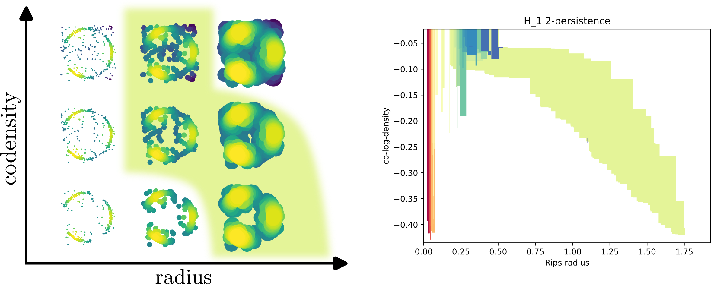
Figure 1: Example of candidate decomposition computed by MMA on a point cloud filtered by both growing balls around the points (also called Čech filtration) and using the sublevel sets of codensity (or, equivalently, the superlevel sets of density), in homology dimension 1. One can see that there is a large lightgreen summand in the candidate decomposition on the right that corresponds to the cycle formed by the points amid outliers, which is also highlighted in lightgreen in the multi-parameter filtration on the left.

An important input parameter of our method MMA is the so-called matching function $\sigma$, which has a large influence on the candidate decompositions produced by MMA. While the output of MMA is only an approximation of the underlying module ${\mathbb{M}}$, we hypothesize that, in the general case, the family $\mathcal{F}$ of candidate decompositions obtained from MMA by varying the matching function parameter across an appropriate family of matching functions $\Sigma$, as $\mathcal{F}=\{\texttt{MMA}{}({\mathbb{M}},L_{\delta},\sigma)\}_{\sigma\in\Sigma,\delta>0}$ , is a complete invariant of the underlying module ${\mathbb{M}}$. We leave this conjecture open for future work.

Related work.

The most common topological invariants of multi-parameter persistence modules are the so-called Hilbert function ${\rm HF}$ and rank invariant ${\rm RI}$. The Hilbert function simply gathers the dimensions of all vector spaces in the module ${\rm HF}=x\mapsto{\rm dim}(H_{*}(S_{x}))$, i.e., it counts the number of topological structures that are present in $S_{x}$ at index $x$, while the rank invariant gathers the ranks of all morphisms in the module ${\rm RI}=(x,y)\mapsto{\rm rank}(H_{*}(S_{x})\to H_{*}(S_{y}))$ (if $x\leq_{n}y$), i.e., it counts the topological structures that are preserved when going from index $x$ to index $y$. The rank invariant is equivalent to computing the persistence barcodes associated to all possible lines in $\mathbb{R}^{n}$; this slicing process is usually referred to as the fibered barcode. The Hilbert function, the rank invariant and the fibered barcode can all be computed with the Rivet software [LW15] in $O(N^{3}\kappa+(N+{\rm log}\kappa)\kappa^{2})$ operations, where $N$ is the number of simplices, and $\kappa$ is the number of indices on which ${\rm HF}$ and ${\rm RI}$ are evaluated. Note that Hilbert functions and rank invariants can also be decomposed themselves in order to be more visually interpretable—the corresponding invariants are called signed barcodes [BOO21].

Unfortunately, Rivet is currently limited to at most $n=2$ filtrations. Moreover, invariants based on dimensions and ranks are known to miss a lot of the structural properties of modules: it is quite easy to find examples of distinct modules that share the same Hilbert function and rank invariant [Vip20a, Figure 3]. Thus, generalizations of the Hilbert function, the rank invariant, the signed barcodes, and their corresponding algorithms, have been introduced recently [DKM22, KM18]. To our knowledge, there is however no corresponding available implementations of these tools.

Finally, another recent line of work also provides candidate decompositions into simple summands for modules that are computed from point cloud data. These decompositions are obtained from applying the elder rule and called the elder-rule staircodes [CKMW20], with running time $O(m^{2}\log(m))$ where $m$ is the number of points of the point cloud. This approach has been shown to be to be theoretically close to the true decomposition, but only works in homology dimension 0 and for $n=2$ parameters.

Hence, computing candidate decompositions for multi-parameter persistence modules indexed over $\mathbb{R}^{n}$ for arbitrary $n\in\mathbb{N}^{*}$ with controlled complexity, running time, and approximation error is still an open and important question, which we tackle in this article using our approximation scheme MMA.

Outline.

Section 2 provides a concise review of multi-parameter persistence modules. In Section 3, we present our new invariants for multi-parameter persistence modules and their approximation properties. Then, we introduce our corresponding algorithm MMA and its stability properties in Section 4. We also discuss the choice of its input parameters in Section 5. Finally, we illustrate the performances of MMA in Section 6.

2 Background

In this section, we recall the basics of multi-parameter persistence modules. This section only contains the necessary background and notations, and can be skipped if the reader is already familiar with persistence theory. A more complete treatment of persistence modules can be found in [CdSGO16, DW22, Oud15].

Multi-parameter persistence modules.

In their most general form, multi-parameter persistence modules are nothing but $k$-vector spaces (where $k$ denotes a field) indexed by $\mathbb{R}^{n}$ and connected by linear maps.

Definition 2.1 (Multi-parameter persistence module).

An ($n$-)multi-parameter persistence module ${\mathbb{M}}$ is a family of vector spaces indexed over $\mathbb{R}^{n}$: ${\mathbb{M}}=\{M_{x}\}_{x\in\mathbb{R}^{n}}$, equipped with linear transformations $\{\varphi_{x}^{y}:M_{x}\rightarrow M_{y}\}_{x,y\in\mathbb{R}^{n},x\leq_{n}y}$, that are called the transition maps of ${\mathbb{M}}$, and that satisfy $\varphi_{x}^{z}=\varphi_{y}^{z}\circ\varphi_{x}^{y}$ for any $x\leq_{n}y\leq_{n}z$.

A morphism between two multi-parameter persistence modules ${\mathbb{M}},{\mathbb{M}}^{\prime}$ with transition maps $\varphi^{\cdot}_{\cdot}$ and $\psi^{\cdot}_{\cdot}$ respectively, is a collection of linear maps $f=\{f_{x}:M_{x}\rightarrow M^{\prime}_{x}\}_{x\in\mathbb{R}^{n}}$, that commutes with transitions maps, i.e., one has $f_{y}\circ\varphi^{y}_{x}=\psi^{y}_{x}\circ f_{x}$, for all $x\leq_{n}y$.

In this article, all multi-parameter persistence modules come from applying the homology functor $H_{*}$ on a multi-parameter filtration of a simplicial complex $S$, that is, on a family $\{S_{x}\}_{x\in\mathbb{R}^{n}}$ of subsets of $S$ indexed over $\mathbb{R}^{n}$ such that $x\leq_{n}y\Rightarrow S_{x}\subseteq S_{y}$. In other words, we study modules of the form ${\mathbb{M}}:=\{H_{*}(S_{x})\}_{x\in\mathbb{R}^{n}}$, where the linear maps $H_{*}(S_{x})\to H_{*}(S_{y})$ are induced by the canonical inclusions $S_{x}\subseteq S_{y}$ (when $x\leq_{n}y$). There are many interesting multi-parameter filtrations in data science; one of the most common one (with $n=2$) comes from filtering by feature scale and density. This allows to detect the topological structures (encoded in the homology groups) of point clouds in the face of noise and outliers [BL20, CB20].

Definition 2.2.

The direct sum of two multi-parameter persistence modules ${\mathbb{M}}$ and ${\mathbb{M}}^{\prime}$, written as ${\mathbb{M}}\oplus{\mathbb{M}}^{\prime}$, is the module ${\mathbb{M}}^{\prime\prime}$ with vector spaces $\{M^{\prime\prime}_{x}\}_{x\in\mathbb{R}^{n}}$ and transition maps $(\phi^{\prime\prime})_{\cdot}^{\cdot}$, defined as $M^{\prime\prime}_{x}=M_{x}\oplus M^{\prime}_{x}$ for all $x\in\mathbb{R}^{n}$, and $(\phi^{\prime\prime})_{\cdot}^{\cdot}=\phi_{\cdot}^{\cdot}\oplus(\phi^{\prime})_{\cdot}^{\cdot}$, where $\{M_{x}\}_{x\in\mathbb{R}^{n}}$ (resp. $\{M^{\prime}_{x}\}_{x\in\mathbb{R}^{n}}$) and $\phi_{\cdot}^{\cdot}$ (resp. $(\phi^{\prime})_{\cdot}^{\cdot}$) are the vector spaces and transition maps of ${\mathbb{M}}$ (resp. ${\mathbb{M}}^{\prime}$) respectively.

A multi-parameter persistence module ${\mathbb{M}}$ such that there are no modules $A$ and $B$ such that ${\mathbb{M}}\simeq A\oplus B$ is called indecomposable.

Note that while multi-parameter persistence modules can always be decomposed into indecomposable summands (see [DX22] for a corresponding algorithm), these summands can be arbitrarily complicated, and the resulting decomposition cannot really be used as an intuitive and simple invariant of the module.

Distances between modules.

Multi-parameter persistence modules can be compared with the standard interleaving distance [Les15].

Definition 2.3 (Interleaving distance).

Given $\varepsilon>0$, two multi-parameter persistence modules ${\mathbb{M}}$ and ${\mathbb{M}}^{\prime}$ are $\boldsymbol{\varepsilon}$-interleaved if there exist two morphisms $f\colon{\mathbb{M}}\to{\mathbb{M}}^{\prime}(\boldsymbol{\varepsilon})$ and $g\colon{\mathbb{M}}^{\prime}\to{\mathbb{M}}(\boldsymbol{\varepsilon})$ such that $g_{\cdot+\boldsymbol{\varepsilon}}\circ f_{\cdot}=\varphi_{\cdot}^{\cdot+2\boldsymbol{\varepsilon}}\text{ and }f_{\cdot+\boldsymbol{\varepsilon}}\circ g_{\cdot}=\psi_{\cdot}^{\cdot+2\boldsymbol{\varepsilon}},$ where ${\mathbb{M}}(\boldsymbol{\varepsilon})$ is the shifted module $\{M_{x+\boldsymbol{\varepsilon}}\}_{x\in\mathbb{R}^{n}}$, $\boldsymbol{\varepsilon}=(\varepsilon,\dots,\varepsilon)\in\mathbb{R}^{n}$, and $\varphi$ and $\psi$ are the transition maps of ${\mathbb{M}}$ and ${\mathbb{M}}^{\prime}$ respectively.

The interleaving distance between two multi-parameter persistence modules ${\mathbb{M}}$ and ${\mathbb{M}}^{\prime}$ is then defined as ${d_{\rm I}}({\mathbb{M}},{\mathbb{M}}^{\prime}):=\inf\left\{\varepsilon\geq 0:{\mathbb{M}}\text{ and }{\mathbb{M}}^{\prime}\text{ are }\boldsymbol{\varepsilon}\text{-interleaved}\right\}.$

The main property of this distance is that it is stable for multi-parameter filtrations that are obtained from the sublevel sets of functions. More precisely, given two continuous functions $f,g:S\to\mathbb{R}^{n}$ defined on a simplicial complex $S$, and such that $\tau\subseteq\sigma\Rightarrow f(\tau)\leq_{n}f(\sigma)$ for any $\tau,\sigma\in S$ (and similarly for $g$), let ${\mathbb{M}}(f),{\mathbb{M}}(g)$ denote the multi-parameter persistence modules obtained from the corresponding multi-parameter filtrations $\{S^{f}_{x}:=\{\sigma\in S:f(\sigma)\leq_{n}x\}\}_{x\in\mathbb{R}^{n}}$ and $\{S_{x}^{g}:=\{\sigma\in S:g(\sigma)\leq_{n}x\}\}_{x\in\mathbb{R}^{n}}$. Then, one has [Les15, Theorem 5.3]:

$${d_{\rm I}}({\mathbb{M}}(f),{\mathbb{M}}(g))\leq\left\lVert f-g\right\rVert_{\infty}.$$ (1)

Another usual distance is the bottleneck distance [BL18, Section 2.3]. Intuitively, it relies on decompositions of the modules into direct sums of indecomposable summands, and is defined as the largest interleaving distance between summands that are matched under some matching.

Definition 2.4 (Bottleneck distance).

Given two multisets $A$ and $B$, $\mu\colon A\not\to B$ is called a matching if there exist $A^{\prime}\subseteq A$ and $B^{\prime}\subseteq B$ such that $\mu\colon A^{\prime}\to B^{\prime}$ is a bijection. The subset $A^{\prime}:=\mathrm{coim}(\mu)$ (resp. $B^{\prime}:=\mathrm{im}(\mu)$) is called the coimage (resp. image) of $\mu$.

Let ${\mathbb{M}}\cong\bigoplus_{i\in\mathcal{I}}M_{i}$ and ${\mathbb{M}}^{\prime}\cong\bigoplus_{j\in\mathcal{J}}M^{\prime}_{j}$ be two multi-parameter persistence modules. Given $\varepsilon\geq 0$, the modules ${\mathbb{M}}$ and ${\mathbb{M}}^{\prime}$ are $\boldsymbol{\varepsilon}$-matched if there exists a matching $\mu\colon\mathcal{I}\not\to\mathcal{J}$ such that $M_{i}$ and $M^{\prime}_{\mu(i)}$ are $\boldsymbol{\varepsilon}$-interleaved for all $i\in\mathrm{coim}(\mu)$, and $M_{i}$ (resp. $M^{\prime}_{j}$) is $\boldsymbol{\varepsilon}$-interleaved with the null module 0 for all $i\in\mathcal{I}\backslash\mathrm{coim}(\mu)$ (resp. $j\in\mathcal{J}\backslash\mathrm{im}(\mu)$).

The bottleneck distance between two multi-parameter persistence modules ${\mathbb{M}}$ and ${\mathbb{M}}^{\prime}$ is then defined as ${d_{\rm B}}({\mathbb{M}},{\mathbb{M}}^{\prime}):=\inf\left\{\varepsilon\geq 0\,:\,{\mathbb{M}}\text{ and }{\mathbb{M}}^{\prime}\text{ are }\boldsymbol{\varepsilon}\text{-matched}\right\}.$

Since a matching between the decompositions of two multi-parameter persistence modules induces an interleaving between the modules themselves, it follows that ${d_{\rm I}}\leq{d_{\rm B}}$. Note also that ${d_{\rm B}}$ can actually be arbitrarily larger than ${d_{\rm I}}$, as showcased in [BL18, Section 9].

Interval modules.

Our approximation result presented in Section 4.2 is stated for modules that can be decomposed into so-called interval modules. Hence, in this section, we define such interval modules. Intuitively, they are modules that are trivial, except on a subset of $\mathbb{R}^{n}$ called an interval.

Definition 2.5 (Interval).

A subset $I$ of $\mathbb{R}^{n}$ is called an interval if it satisfies:

• (convexity) if $p,q\in I$ and $p\leq_{n}r\leq_{n}q$ then $r\in I$, and

• (connectivity) if $p,q\in I$, then there exists a finite sequence $r_{1},r_{2},\dots,r_{m}\in I,$ for some $m\in\mathbb{N}$, such that $p\sim r_{1}\sim r_{2}\sim\dots\sim r_{m}\sim q$, where $\sim$ can be either $\leq_{n}$ or $\geq_{n}$.

Definition 2.6 (Indicator module, Interval module).

A multi-parameter persistence module ${\mathbb{M}}$ is an indicator module if there exists a set $S\subseteq\mathbb{R}^{n}$, called the support of ${\mathbb{M}}$ and denoted by ${\rm supp}({\mathbb{M}})$, such that:

$$\forall x\in\mathbb{R}^{n},\,M_{x}=\begin{cases}k\text{ if }x\in S\\ {\bf 0}\text{ otherwise}\end{cases}\ \ \ {\rm and}\ \ \ \,\forall x,y\in\mathbb{R}^{n},\,\varphi_{x}^{y}=\begin{cases}\mathrm{id}_{k\rightarrow k}\text{ if }x\leq_{n}y\in S\\ 0\text{ otherwise}\end{cases}$$

where $\varphi_{\cdot}^{\cdot}$ are the transition maps of ${\mathbb{M}}$. If $S$ is an interval, ${\mathbb{M}}$ is called an interval module.

Finally, we define a specific type of interval modules, those whose support is equal to a union of rectangles. We call these modules discretely presented—the stable candidate decompositions computed by our algorithm MMA in Section 4 are actually made up of such modules.

Definition 2.7 (Discretely presented interval module).

An interval module $I$ is discretely presented if its support is a locally finite union of rectangles in $\overline{\mathbb{R}}^{n}$, and whose boundary is an $(n-1)$-submanifold of $\mathbb{R}^{n}$. More precisely, there exist two locally finite families of points, the birth and death critical points of $I$, denoted by $C_{B}(I)$ and $C_{D}(I)$ respectively, such that:

$$I:=\mathrm{\mathbf{Int}}\left(\bigcup_{c\in C_{B}(I)}\bigcup_{c^{\prime}\in C_{D}(I)}R_{c,c^{\prime}}\right),$$ (2)

where $R_{c,c^{\prime}}:=\{x\in\mathbb{R}^{n}:c\leq_{n}x\leq_{n}c^{\prime}\}$ is the rectangle defined by corners $c$ and $c^{\prime}$, and $\mathrm{\mathbf{Int}}\left(S\right)$ (where $S$ is an interval) denotes the interval module whose support is $S$.

Note that when only one filtration is given, single-parameter persistence modules always decompose into interval modules: ${\mathbb{M}}\cong\bigoplus_{i\in\mathcal{I}}\mathrm{\mathbf{Int}}\left([b_{i},d_{i}]\right)$ [CdSGO16, Theorem 2.8]. In that case, they are frequently represented as the collection of the interval supports (in $\mathbb{R}$) of their summands, also called persistence barcode ${\mathcal{B}}({\mathbb{M}}):=\{[b_{i},d_{i}]\}_{i\in\mathcal{I}}$.

Fibered barcode.

The fibered barcode [LW15] is a centerpiece of our approximation scheme, and is defined, given a multi-parameter persistence module ${\mathbb{M}}$, as a map that takes as input a line (or segment) $l$ in $\mathbb{R}^{n}$, and outputs the persistence barcode associated to the single-parameter persistence module obtained by restricting ${\mathbb{M}}$ along $l$. Hence, in the following, we formalize the intersections between multi-parameter persistence modules and lines in $\mathbb{R}^{n}$.

Definition 2.8 (Fibered Barcode).

Let ${\mathbb{M}}$ be a pointwise finite-dimensional multi-parameter persistence module. Given a discrete family of diagonal lines $L\subseteq\mathcal{L}$ (i.e., lines with direction vector $(1,\dots,1)\in\mathbb{R}^{n}$), we let the $L$-fibered barcode (or fibered barcode for short when $L$ is clear) be the family of barcodes associated to restrictions of the module to lines in $L$, i.e., ${\mathcal{F}}{\mathcal{B}}({\mathbb{M}})_{L}=\{{\mathcal{B}}({\left.\kern-1.2pt{\mathbb{M}}\vphantom{\big{|}}\right|_{l}}):l\in L\}$.

Remark 2.9.

Recall from single-parameter persistence theory that the support of the restriction of ${\mathbb{M}}$ to $l$ is a set of bars called persistence barcode: ${\mathcal{B}}({\left.\kern-1.2pt{\mathbb{M}}\vphantom{\big{|}}\right|_{l}})={\rm supp}({\left.\kern-1.2pt{\mathbb{M}}\vphantom{\big{|}}\right|_{l}})=\{[b_{i},d_{i}]\}_{i\in\mathcal{I}(l)}$, where $\mathcal{I}(l)$ is an index set that depends on ${\mathbb{M}}$ and $l$. Moreover, when ${\mathbb{M}}=\bigoplus_{i\in\mathcal{I}}I_{i}$ is decomposable into interval modules, there are as many bars in the barcode as there are interval summands intersecting the line ${\mathcal{B}}({\left.\kern-1.2pt{\mathbb{M}}\vphantom{\big{|}}\right|_{l}})=\{{\rm supp}({\left.\kern-1.2ptI_{i}\vphantom{\big{|}}\right|_{l}})\}_{i\in\mathcal{I}}$.

It is also useful to characterize the fibered barcode with endpoints of lines.

Definition 2.10 (Birthpoint, Deathpoint).

Given a point $x\in\mathbb{R}^{n}$ and an interval module $I$, we call $b_{x}^{I}:=\min\left\{x+\boldsymbol{\delta}\,:\,\delta\in\mathbb{R}\right\}$ (resp. $d_{x}^{I}=\max\left\{x+\boldsymbol{\delta}\,:\,\delta\in\mathbb{R}\right\}$) the birthpoint (resp. deathpoint) associated to $x$ and $I$, where $\boldsymbol{\delta}=(\delta,\dots,\delta)\in\mathbb{R}^{n}$.

Similarly, given a diagonal line $l\subseteq\mathbb{R}^{n}$, we define the birthpoint (resp. deathpoint) associated to $l$ and $I$ as $b_{l}^{I}:=b_{x}^{I}$ (resp. $d_{l}^{I}:=d_{x}^{I}$) for any $x\in l$. See Figure 2

Remark 2.11.

Using birthpoints and deathpoints, the $L$-fibered barcode of an interval decomposable multi-parameter persistence module ${\mathbb{M}}=\bigoplus_{i\in\mathcal{I}}I_{i}$ is written as:

$${\mathcal{F}}{\mathcal{B}}({\mathbb{M}})_{L}=\{{\mathcal{B}}({\left.\kern-1.2pt{\mathbb{M}}\vphantom{\big{|}}\right|_{l}}):l\in L\}=\{([b^{I_{i}}_{l},d^{I_{i}}_{l}])_{i\in\mathcal{I}}:l\in L\}.$$ (3)

3 Approximate candidate decompositions

In this section, we present our family of topological invariants for multi-parameter persistence modules, defined as candidate decompositions into interval summands, in Section 3.1. We then prove their approximation guarantees in Section 3.2.

3.1 Candidate modules and interval decompositions

In this section, given a multi-parameter persistence module ${\mathbb{M}}$, we define a family of good proxies for ${\mathbb{M}}$ (see Definition 3.3), called candidate decompositions. These candidate decompositions are multi-parameter persistence modules that can be decomposed into intervals summands, and approximate ${\mathbb{M}}$ well when ${\mathbb{M}}$ is interval decomposable itself, in the sense that ${d_{\rm I}}({\mathbb{M}},\tilde{\mathbb{M}})$ and ${d_{\rm B}}({\mathbb{M}},\tilde{\mathbb{M}})$ are upper bounded for any candidate decomposition $\tilde{\mathbb{M}}$. Practical computations of instances of such candidate decompositions can be done with our MMA algorithm, that we provide in Section 4.2.

(Exact) matchings and grids of lines.

Our candidate decompositions depend on so-called matching functions and $\delta$-grids of lines, that we now define.

Definition 3.1 ((Exact) matching).

Let ${\mathbb{M}}$ be a multi-parameter persistence module. Let $l,l^{\prime}$ be two lines in $\mathbb{R}^{n}$. A map $\sigma$ between the persistence barcodes $\sigma\colon{\mathcal{B}}({\left.\kern-1.2pt{\mathbb{M}}\vphantom{\big{|}}\right|_{l}})\rightarrow{\mathcal{B}}({\left.\kern-1.2pt{\mathbb{M}}\vphantom{\big{|}}\right|_{l^{\prime}}})\cup\left\{\varnothing\right\}$ is called an (${\mathbb{M}}$-)matching between $l$ and $l^{\prime}$ if the restriction of $\sigma$ to $\sigma^{-1}({\mathcal{B}}({\left.\kern-1.2pt{\mathbb{M}}\vphantom{\big{|}}\right|_{l^{\prime}}}))$ is injective.

Furthermore, if ${\mathbb{M}}$ is interval decomposable, ${\mathbb{M}}=\bigoplus_{i\in\mathcal{I}}I_{i}$, we let $\iota_{1}:{\mathcal{B}}({\left.\kern-1.2pt{\mathbb{M}}\vphantom{\big{|}}\right|_{l}})\rightarrow\mathcal{I}$ and $\iota_{2}:{\mathcal{B}}({\left.\kern-1.2pt{\mathbb{M}}\vphantom{\big{|}}\right|_{l^{\prime}}})\rightarrow\mathcal{I}$ be maps that retrieve the indices of the summands corresponding to the bars in ${\mathcal{B}}({\left.\kern-1.2pt{\mathbb{M}}\vphantom{\big{|}}\right|_{l^{\prime}}})$ and ${\mathcal{B}}({\left.\kern-1.2pt{\mathbb{M}}\vphantom{\big{|}}\right|_{l^{\prime}}})$ as per Equation (3). Then, $\sigma$ is said to be exact if $\iota_{1}(b)=\iota_{2}(\sigma(b))$ for any bar $b\in\sigma^{-1}({\mathcal{B}}({\left.\kern-1.2pt{\mathbb{M}}\vphantom{\big{|}}\right|_{l^{\prime}}}))$. In other words, bars that are matched under $\sigma$ correspond to the same underlying interval summand of ${\mathbb{M}}$. Note that the interval decomposition of ${\mathbb{M}}$ always induces a canonical exact matching, that we denote $\sigma_{\mathbb{M}}$.

Definition 3.2 ($\delta$-grid of lines).

Let $K\subset\mathbb{R}^{n}$ be a compact set and $\delta>0$. The $\delta$-grid of lines associated to $K$, denoted as $L_{\delta}(K)$, is a family of diagonal lines evenly sampled in $K$:

$$L_{\delta}(K):=\{l_{\delta\cdot u}:u\in\mathbb{Z}^{n}\text{ and }l_{\delta\cdot u}\cap K\neq\varnothing\},$$

where $l_{\delta\cdot u}:=\delta\cdot u+\boldsymbol{e}_{\Delta}$ is the diagonal line with direction vector $\boldsymbol{e}_{\Delta}=[1,\dots,1]^{T}\in\mathbb{R}^{n}$ passing through $\delta\cdot u$.

Candidates decompositions.

Our candidate decompositions are, roughly speaking, modules with the same fibered barcodes than ${\mathbb{M}}$ on a $\delta$-grid of lines. When ${\mathbb{M}}$ is interval decomposable, we also ask the exact matchings induced by the candidate decompositions to commute with the one induced by ${\mathbb{M}}$ (we discuss such matchings in Section 4.4).

Definition 3.3 (Candidate).

Let ${\mathbb{M}}$ be a multi-parameter persistence module. Let $K$ be a hyperrectangle in $\mathbb{R}^{n}$ containing the multigraded Betti numbers of ${\mathbb{M}}$ , and $L:=L_{\delta}(K^{\delta})$ be the $\delta$-grid of lines of the offset $K^{\delta}=\{x\in\mathbb{R}^{n}:d_{\infty}(x,K)\leq\delta\}$, where $d_{\infty}$ stands for the $\left\lVert\cdot\right\rVert_{\infty}$ distance. A multi-parameter persistence module $\tilde{\mathbb{M}}_{\delta}$ is called a $\delta$-candidate decomposition of ${\mathbb{M}}$ if

1. $\tilde{\mathbb{M}}_{\delta}$ is interval decomposable: $\tilde{\mathbb{M}}_{\delta}=\bigoplus_{i\in\tilde{\mathcal{I}}}\tilde{I}_{i}$,

2. ${\mathcal{B}}({\left.\kern-1.2pt{\mathbb{M}}\vphantom{\big{|}}\right|_{l}})={\mathcal{B}}({\left.\kern-1.2pt\tilde{\mathbb{M}}_{\delta}\vphantom{\big{|}}\right|_{l}})$ for any $l\in L$, i.e., their $L$-fibered barcodes are the same, and

3. if ${\mathbb{M}}=\bigoplus_{i\in\mathcal{I}}I_{i}$ is interval decomposable, then there exists a bijection $\nu\colon\mathcal{I}_{L}\to\tilde{\mathcal{I}}$, where $\mathcal{I}_{L}=\{i\in\mathcal{I}:I_{i}\cap L\neq\varnothing\}$, such that ${\rm supp}({\left.\kern-1.2ptI_{i}\vphantom{\big{|}}\right|_{l}})={\rm supp}({\left.\kern-1.2pt\tilde{I}_{\nu(i)}\vphantom{\big{|}}\right|_{l}})$, for any $i\in\mathcal{I}_{L}$ and $l\in L$. In particular, for any two lines $l,l^{\prime}\in L$, the following diagram commutes:

   where $\nu_{l}\colon{\left.\kern-1.2ptI_{i}\vphantom{\big{|}}\right|_{l}}\in{\mathcal{B}}({\left.\kern-1.2pt{\mathbb{M}}\vphantom{\big{|}}\right|_{l}})\mapsto{\left.\kern-1.2pt\tilde{I}_{\nu(i)}\vphantom{\big{|}}\right|_{l}}\in{\mathcal{B}}({\left.\kern-1.2pt\tilde{\mathbb{M}}_{\delta}\vphantom{\big{|}}\right|_{l}})$ (and similarly for $l^{\prime}$). In other words, ${\mathbb{M}}$ and $\tilde{\mathbb{M}}_{\delta}$ have the same matched barcodes along the lines of $L$, up to interval reordering.

We now claim that multi-parameter persistence modules that are $\delta$-candidate decompositions of a given interval decomposable multi-parameter persistence module ${\mathbb{M}}$ are $\delta$ close to ${\mathbb{M}}$ in $K$, as stated in the following approximation result, which we prove in the next section.

Proposition 3.4 (Approximation result).

Let ${\mathbb{M}}$ be an interval decomposable multi-parameter persistence module. Then, any $\delta$-candidate decomposition $\tilde{\mathbb{M}}_{\delta}$ of ${\mathbb{M}}$ satisfies

$${d_{\rm I}}(\tilde{\mathbb{M}}_{\delta}\cap K,{\mathbb{M}}\cap K)\leq{d_{\rm B}}(\tilde{\mathbb{M}}_{\delta}\cap K,{\mathbb{M}}\cap K)\leq\delta,$$

where ${\mathbb{M}}\cap K$ stands for the module that is isomorphic to ${\mathbb{M}}$ on $K$ and the null module outside of $K$.

Note that it is possible to generalize Proposition 3.4 to modules that are not restricted to $K$ by constraining the parts of the candidate decompositions that are outside of $K$ with Kan extensions, but we stick to our formulation for the sake of simplicity.

3.2 Proof of Proposition 3.4

In this section, we prove Proposition 3.4. This section is quite technical and can thus be skipped by readers who are most interested in the general exposition. We first provide several additional definitions in Section 3.2.1, that are a bit technical yet convenient for writing down the subsequent proofs. Then, we prove a few technical results and lemmas in Section 3.2.2, and we finally prove Proposition 3.4 in Section 3.2.3.

Notations.

We first introduce a few notations: we let $(e_{1},\dots,e_{n})$ be the canonical basis of $\mathbb{R}^{n}$, and, given a set $A\subseteq\mathbb{R}^{n}$, we let ${\rm conv}(A)$ denote the convex hull of $A$. Moreover, given a hyperplane $H\subseteq\mathbb{R}^{n}$ and its two associated vectors $a_{H},b_{H}\in\mathbb{R}^{n}$ which satisfy $H=b_{H}+\{x\in\mathbb{R}^{n}:\langle x,a_{H}\rangle=0\}$, we call $a_{H}$ the codirection of $H$. When $a_{H}$ is a vector in the canonical basis of $\mathbb{R}^{n}$, i.e., there exists $i\in\llbracket 1,n\rrbracket$ such that $a_{H}=e_{i}$, we slightly abuse notation and also call $i$ the codirection of $H$.

3.2.1 Boundaries, facets and diagonal lines

In this section, we define the upper- and lower-boundaries of interval modules, as well as their so-called facets, which are convenient characterizations of the interval supports.

Definition 3.5 (Upper- and lower-boundaries).

Given an interval $I$, its upper-boundary $U[I]$ and lower-boundary $L[I]$ are defined as:

$$L[I]:=\left\{x\in\bar{I}:\forall y\in\mathbb{R}^{n},\,y<_{n}x\Rightarrow y\not\in I\right\},\ \ U[I]:=\left\{x\in\bar{I}:\forall y\in\mathbb{R}^{n},\,y>_{n}x\Rightarrow y\not\in I\right\}$$

Moreover, the boundary of ${\rm supp}(I)$ can be decomposed with $\partial{\rm supp}(I)=L[I]\cup U[I]$. See Figure 2 for an illustration.

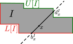
Figure 2: Lower- and upper-boundaries of a 2-interval (Definition 3.5); and birthpoints and deathpoints $b_{x}^{I}$ and $d_{x}^{I}$ (Definition 2.10) of a point $x\in\mathbb{R}^{2}$.

When interval modules are discretely presented (see Definition 2.7), their lower- and upper-boundaries are made of flat parts, which are the faces of the corresponding rectangles forming the interval. Hence, we call facets the subsets of the lower- and upper-boundaries that are included in some hyperplanes of $\mathbb{R}^{n}$.

Definition 3.6 (Facet).

A lower (resp. upper) facet of an interval $I$ is an $(n-1)$-submanifold of $\partial{\rm supp}(I)$ written as $\left\{x\in\mathbb{R}^{n}\,:\,x_{i}=c\right\}\cap L[I]$ (resp. $\left\{x\in\mathbb{R}^{n}\,:\,x_{i}=c\right\}\cap U[I]$) for some $c\in\mathbb{R}$ and some dimension $i\in\llbracket 1,n\rrbracket$ that is called the facet codirection. In particular, the upper- and lower-boundaries of a discretely presented interval module is a locally finite union of facets.

We end this section by defining some properties of diagonal lines.

Definition 3.7 ($\delta$-regularly distributed lines filling a compact set).

Let $L$ be a set of diagonal lines in $\mathbb{R}^{n}$ and $K\subseteq\mathbb{R}^{n}$ be a compact set. Then, we say that :

1. two diagonal lines $l,l^{\prime}\in L$ are $\delta$-consecutive (or consecutive when $\delta$ is clear) if there exists ${\overrightarrow{u}}\in\left\{0,1\right\}^{n}\backslash\left\{\mathbf{0},\mathbf{1}\right\}$ such that $l^{\prime}=l\pm\delta\cdot{\overrightarrow{u}}$.

2. two diagonal lines $l,l^{\prime}\in L$ are $\delta$-comparable if there exists a positive or negative vector $\overrightarrow{u}\in\mathbb{R}^{n}$ (i.e. a vector whose coordinates are all positive or all negative) with $\left\lVert\overrightarrow{u}\right\rVert_{\infty}\leq\delta$ such that $l^{\prime}=l+\overrightarrow{u}$. If $\overrightarrow{u}$ is positive (resp. negative), we write $l^{\prime}\geq l$ (resp. $l^{\prime}\leq l$).

3. $L$ is $\delta$-regularly distributed if, for any pair of lines $(l,l^{\prime})\in L$, there exists a sequence of $\delta$-consecutive lines $\{l_{1},\dots,l_{k}\}$ in $L$ such that $l=l_{1}$ and $l^{\prime}=l_{k}$.

4. for a given line $l$ in a $\delta$-regularly distributed family of lines $L$, we call $L_{l}:=L\cap\{l+\delta\cdot\overrightarrow{u}:\overrightarrow{u}\in\{0,1\}^{n-1}\times\{0\}\}$ the $L$-surrounding set of $l$. In particular, one has $|L_{l}|\leq 2^{n-1}$.

5. $L$ $\delta$-fills $K$ (or fills $K$ when $\delta$ is clear) if any point of $K$ is at distance at most $\delta/2$ from some line in $L$. More formally, $K$ is included in the offset $L^{\delta/2}$.

Remark 3.8.

One can check that the $\delta$-grid of lines of a hyperrectangle $K$ (used in Definition 3.3) is $\delta$-regularly distributed and $\delta$-fills $K$.

3.2.2 Additional lemmas

In this section, we prove a few preliminary results about endpoints of interval modules, that will turn out useful for proving Proposition 3.4. The first simple, yet fundamental lemma that we will use repeatedly states that endpoints of interval modules cannot be comparable.

Lemma 3.9.

Let $l_{1},l_{2}$ be two diagonal lines and $I$ be an interval module such that the barcodes ${\mathcal{B}}({\left.\kern-1.2ptI\vphantom{\big{|}}\right|_{l_{1}}})$ and ${\mathcal{B}}({\left.\kern-1.2ptI\vphantom{\big{|}}\right|_{l_{2}}})$ are not empty. Let ${\mathcal{B}}({\left.\kern-1.2ptI\vphantom{\big{|}}\right|_{l_{1}}})=[b_{1},d_{1}]$ and ${\mathcal{B}}({\left.\kern-1.2ptI\vphantom{\big{|}}\right|_{l_{2}}})=[b_{2},d_{2}]$. Then $b_{1}$ and $b_{2}$ are not comparable, i.e., $b_{1}\not\leq_{n}b_{2}$ and $b_{1}\not\geq_{n}b_{2}$. The same is true for $d_{1}$ and $d_{2}$. In other words, the rectangles $R_{b_{1},b_{2}}$, $R_{b_{2},b_{1}}$, $R_{d_{1},d_{2}}$ and $R_{d_{2},d_{1}}$ are flat (i.e., one side has length 0).

Proof.

This lemma is a simple consequence of the persistence module definition: if $b_{1}$ and $b_{2}$ were comparable (as in Figure 3), then the rectangle $R_{b_{1},b_{2}}$ would not be trivial, and $b_{2}$ would not be a birthpoint since it would be possible to find a smaller birthpoint $\tilde{b}_{2}\leq_{n}b_{2}$ w.r.t. the partial order of $\mathbb{R}^{n}$ along the diagonal line passing through $b_{2}$. A similar argument holds for $d_{1}$ and $d_{2}$. See Figure 3.

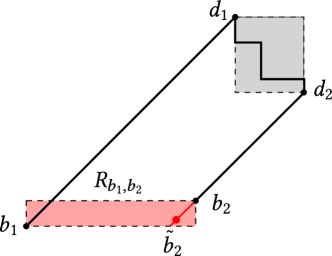
Figure 3: Two bars $[b_{1},d_{1}]$ and $[b_{2},d_{2}]$ of an interval module.

∎

Stability of close barcodes.

We now show that endpoints of bars in barcodes from lines that are close should also be close. In other words, bars of the fibered barcode that are associated to lines that are close to each other must have similar length, as stated in the lemma below (see also [Lan18, Lemma 2]).

Lemma 3.10.

Let $I$ be an interval module, let $l_{1},l_{2}\subseteq\mathbb{R}^{n}$ be two diagonal lines and let $\overrightarrow{u}\in\mathbb{R}^{n}$ be a positive or negative vector (i.e., the coordinates of $\overrightarrow{u}$ are either all positive or all negative) such that $l_{2}=l_{1}+\overrightarrow{u}$. Then, the following properties hold:

1. If the barcode ${\mathcal{B}}({\left.\kern-1.2ptI\vphantom{\big{|}}\right|_{l_{1}}})=\{[b^{I}_{l_{1}},d^{I}_{l_{1}}]\}$ is not empty and satisfies $\left\lVert d^{I}_{l_{1}}-b^{I}_{l_{1}}\right\rVert_{\infty}>\left\lVert\overrightarrow{u}\right\rVert_{\infty}$, then the barcode ${\mathcal{B}}({\left.\kern-1.2ptI\vphantom{\big{|}}\right|_{l_{2}}})$ is not empty as well, and

1. If the barcodes ${\mathcal{B}}({\left.\kern-1.2ptI\vphantom{\big{|}}\right|_{l_{1}}})$ and ${\mathcal{B}}({\left.\kern-1.2ptI\vphantom{\big{|}}\right|_{l_{2}}})$ are not empty, then one has

   $$\left\lVert d^{I}_{l_{1}}-d^{I}_{l_{2}}\right\rVert_{\infty}\leq\left\lVert\overrightarrow{u}\right\rVert_{\infty}\text{ and }\left\lVert b^{I}_{l_{1}}-b^{I}_{l_{2}}\right\rVert_{\infty}\leq\left\lVert\overrightarrow{u}\right\rVert_{\infty},$$

   where we used the conventions $(+\boldsymbol{\infty})-(+\boldsymbol{\infty})=(-\boldsymbol{\infty})-(-\boldsymbol{\infty})=0$.

Proof.

Item $(i)$. Since $|(d^{I}_{l_{1}})_{i}-(b^{I}_{l_{1}})_{i}|=\left\lVert d^{I}_{l_{1}}-b^{I}_{l_{1}}\right\rVert_{\infty}>\left\lVert\overrightarrow{u}\right\rVert_{\infty}$ for any index $i\in\llbracket 1,n\rrbracket$, it follows that $b^{I}_{l_{1}}\leq_{n}b^{I}_{l_{1}}+\overrightarrow{u}\leq_{n}d^{I}_{l_{1}}$. Thus $b^{I}_{l_{1}}+\overrightarrow{u}$ must belong to ${\rm supp}(I)$ since $I$ is an interval. Hence, since $b^{I}_{l_{1}}+\overrightarrow{u}\in l_{2}$, one has ${\mathcal{B}}({\left.\kern-1.2ptI\vphantom{\big{|}}\right|_{l_{2}}})={\rm supp}(I)\cap l_{2}\neq\varnothing$.

Item $(ii)$. If one of the endpoints is infinite, the result holds trivially as the other endpoint has to be infinite too, so we now assume that the endpoints of the bars are all finite. Without loss of generality, assume that $l_{2}=l_{1}+\overrightarrow{u}$ where $\overrightarrow{u}$ is positive. Now, since both $d_{l_{2}}^{I}$ and $d_{l_{1}}^{I}+\overrightarrow{u}$ belong to $l_{2}$, they are comparable, so one has either $d_{l_{2}}^{I}>_{n}d_{l_{1}}^{I}+\overrightarrow{u}$ or $d_{l_{2}}^{I}\leq_{n}d_{l_{1}}^{I}+\overrightarrow{u}$. However, the first possibility would lead to $d_{l_{2}}^{I}>_{n}d_{l_{1}}^{I}+\overrightarrow{u}>_{n}d_{l_{1}}^{I}$, hence $d_{l_{1}}^{I}$ and $d_{l_{2}}^{I}$ would be (strictly) comparable in $\mathbb{R}^{n}$, which contradicts Lemma 3.9. Thus, one must have $d_{l_{2}}^{I}\leq_{n}d_{l_{1}}^{I}+\overrightarrow{u}$. Furthermore, and using the exact same arguments, $d^{I}_{l_{2}}-\overrightarrow{u}+\left\lVert\overrightarrow{u}\right\rVert_{\infty}\cdot\boldsymbol{1}$ is on $l_{1}$, and one must have $d_{l_{2}}^{I}-\overrightarrow{u}+\left\lVert\overrightarrow{u}\right\rVert_{\infty}\cdot\boldsymbol{1}\geq_{n}d_{l_{1}}^{I}$. Finally, by combining the two previous inequalities, one has

$$d_{l_{1}}^{I}-\left\lVert\overrightarrow{u}\right\rVert_{\infty}\cdot\textbf{1}\leq_{n}d_{l_{1}}^{I}+\overrightarrow{u}-\left\lVert\overrightarrow{u}\right\rVert_{\infty}\cdot\textbf{1}\leq_{n}d_{l_{2}}^{I}\leq_{n}d_{l_{1}}^{I}+\overrightarrow{u}\leq_{n}d_{l_{1}}^{I}+\left\lVert\overrightarrow{u}\right\rVert_{\infty}\cdot\textbf{1},$$

which leads to the result for deathpoints. The proof extends straightforwardly to birthpoints. ∎

Endpoint location.

The next definition and result show that endpoints of an interval module must be located in the vicinity of the other endpoints of the module that are close to it—more precisely, in their rectangle hull. This will be useful in the proof of Proposition 3.4; in particular, we will use this result to characterize the positions of endpoints of any given diagonal line $l$ solely from the endpoints of the lines of the grid $L$ that are close to $l$.

Definition 3.11.

Let $S\subseteq\mathbb{R}^{n}$. The rectangle hull of $S$, denoted by $\mathrm{recthull}[S]$, is defined as the smallest rectangle containing $S$

$$\mathrm{recthull}[S]:=\left\{x\in\mathbb{R}^{n}:\forall i\in\llbracket 1,n\rrbracket,\min_{s\in S}s_{i}\leq x_{i}\leq\max_{s\in S}s_{i}\right\}=R_{\wedge S,\vee S},$$

where $(\wedge S)_{i}:=\min_{s\in S}s_{i}$ and $(\vee S)_{i}:=\max_{s\in S}s_{i}$.

Lemma 3.12 (Endpoints bound).

Let $I$ be an interval module. Let $K$ be a hyperrectangle and $L=L_{\delta}(K^{\delta})$ be a $\delta$-grid of lines. Let $x\in K$, $l_{x}$ be the diagonal line passing through $x$, and let $L_{x,\delta}:=\{l\in L\,:\,d_{\infty}(x,l)\leq\delta\text{ and }l_{x},l\text{ are $\delta$-comparable}\}$, which is non-empty since $L$ $\delta$-fills $K$. Assume that $l_{x}\cap{\rm supp}(I)\neq\varnothing$, and $d^{I}_{x}\in U[I]$ be the associated deathpoint, and assume that for any line $l$ in $L_{x,\delta}$, one has ${\rm supp}(I)\cap l\neq\varnothing$, and let $D_{x,\delta}^{I}$ be the set of the associated deathpoints: $D_{x,\delta}^{I}=\{d_{l}^{I}\,:\,l\in L_{x,\delta}\}$. Then, $d^{I}_{x}$ belongs to the rectangle hull of a subset $\tilde{D}_{x,\delta}^{I}$ of $D_{x,\delta}^{I}$: one has $d^{I}_{x}\in\mathrm{recthull}[\tilde{D}_{x,\delta}^{I}]$ with $\tilde{D}_{x,\delta}^{I}\subseteq D_{x,\delta}^{I}$.

Similarly, if $b^{I}_{x}\in L[I]$ is a birthpoint, then $b^{I}_{x}\in\mathrm{recthull}[\tilde{B}_{x,\delta}^{I}]$, where $\tilde{B}_{x,\delta}^{I}$ is a subset of $B_{x,\delta}^{I}=\{b_{l}^{I}\,:\,l\in L_{x,\delta}\}$, i.e., the set of birthpoints associated to $L_{x,\delta}$.

In other words, the endpoints of an interval module always belong to the rectangle hull of the endpoints associated to neighbouring lines. See Figure 4 for an illustration.

Figure 4: Example of deathpoint bound in $\mathbb{R}^{3}$, with $d\in U[I]$, and $D_{x,\delta}^{I}=\left\{d_{1},d_{2},d_{3},d_{4}\right\}$. (Left) Rectangle hull of the deathpoints $D_{x,\delta}^{I}$. (Right) Upper-boundary $U[I]$.

Proof.

We first prove the result for deathpoints. Note that the result is trivially satisfied if $d^{I}_{x}$ and the deathpoints in $D^{I}_{x,\delta}$ are infinite, so we assume that they are finite in the following. To alleviate notations, we let $d:=d^{I}_{x}$. Let $j\in\llbracket 1,n\rrbracket$ be an arbitrary dimension. In order to prove the result, we will show that there exist two deathpoints $\underline{d}$ and $\overline{d}$ associated to consecutive lines of $L_{x,\delta}$ such that $\underline{d}_{j}\leq d_{j}\leq\overline{d}_{j}$.

Construction of $\underline{d},\overline{d}$. Let $H_{j}$ be the hyperplane $H_{j}=d+e_{j}^{\perp}$. Since $L$ $\delta$-fills $K$, there exists a diagonal line $l\in L$ such that $d_{\infty}(x,l)\leq\delta/2$. Moreover, since $l$ and $l_{x}$ (the line passing through $x$ and $d$) are both diagonal, one has $d_{\infty}(d,l)=d_{\infty}(x,l)\leq\delta/2$. Let $\pi_{l}(d)\in l$ be the projection of $d$ onto $l$ that achieves $d_{\infty}(d,l)$, and let $d^{j}:=l\cap H_{j}$. See Figure 5 for an illustration of these objects.

Figure 5: Illustration of $H_{j},d,l,d^{j}$.

Since $d^{j}$ and $d$ belong to $H_{j}$, they have the same $j$-th coordinate: $d^{j}_{j}=d_{j}$. Moreover, both $d^{j}$ and $\pi_{l}(d)$ belong to the diagonal line $l$, hence they are comparable, and $\|d^{j}-\pi_{l}(d)\|_{\infty}=|(d^{j}-\pi_{l}(d))_{i}|$ for any $i\in\llbracket 1,n\rrbracket$. Then, one has $\|d^{j}-d\|_{\infty}\leq\|d^{j}-\pi_{l}(d)\|_{\infty}+\|\pi_{l}(d)-d\|_{\infty}=|(d^{j}-\pi_{l}(d))_{j}|+\|\pi_{l}(d)-d\|_{\infty}=|(d-\pi_{l}(d))_{j}|+\|\pi_{l}(d)-d\|_{\infty}\leq 2\|\pi_{l}(d)-d\|_{\infty}\leq\delta$.

Let $d^{+}=d^{j}+\delta\sum_{j\in\mathcal{J}^{\prime\prime}}e_{j}\text{ and }d^{-}=d^{j}-\delta\sum_{j\in\mathcal{J}^{\prime}}e_{j}$, where

$$\mathcal{J}^{\prime}=\left\{i\in\llbracket 1,n\rrbracket\backslash\{j\}:d_{i}<d^{j}_{i}\right\}\text{ and }\mathcal{J}^{\prime\prime}=\left\{i\in\llbracket 1,n\rrbracket\backslash\{j\}:d_{i}>d^{j}_{i}\right\}.$$

By construction, one has $d^{-}\leq d\leq d^{+}\in H_{j}$ and

$$\|d^{+}-d\|_{\infty},\|d^{-}-d\|_{\infty}\leq\delta.$$ (4)

Since $l$ and the diagonal lines $\underline{l}$ and $\overline{l}$ passing through $d^{-}$ and $d^{+}$ respectively are $\delta$-consecutive, and since $x\in K$, the projections of $x$ onto $\underline{l}$ and $\overline{l}$ are in $K^{\delta}$, and thus $\underline{l},\overline{l}$ must belong to $L$, and thus to $L_{x,\delta}$, as by construction $l_{x}$ is $\delta$-comparable with the diagonal lines $\underline{l}$ and $\overline{l}$. Let $\overline{d}:=d_{\underline{l}}^{I}\in\underline{l}$ and $\underline{d}:=d_{\overline{l}}^{I}\in\overline{l}$ be their deathpoints (which exist by assumption).

Proof of inequalities. We now show that $\overline{d}_{j}\geq_{n}d_{j}\geq_{n}\underline{d}_{j}$. We start with the second inequality. Since $d^{+}$ and $\underline{d}$ are one the same diagonal line, they are comparable. Furthermore, if one had $d^{+}<_{n}\underline{d}$ by contradiction, then the induced rectangle $R_{d,\underline{d}}$ would not be flat since $d\leq_{n}d^{+}<_{n}\underline{d}$, which would contradict Lemma 3.9. As a consequence, $d^{+}\geq_{n}\underline{d}$. Taking the $j$-th coordinate yields $d_{j}=d^{+}_{j}\geq\underline{d}_{j}$. The first inequality holds using the same arguments.

This proof applies straightforwardly to birthpoints by symmetry. ∎

Using Lemma 3.10, one can generalize Lemma 3.12 above to the case where some lines in $L_{x,\delta}$ have an empty intersection with ${\rm supp}(I)$, and then define a common location for all endpoints that belong to the convex hull of the same $L$-surrounding set, as we do in the following proposition.

Proposition 3.13.

Let $I$ be an interval module. Let $K$ be a hyperrectangle and $L=L_{\delta}(K^{\delta})$ be a $\delta$-grid of lines. Let $l\in L$ such that $|L_{l}|=2^{n-1}$ and assume that ${\rm conv}(L_{l})\cap L[I]$ (resp. ${\rm conv}(L_{l})\cap U[I]$) is not empty. Then, there exists a set $B_{l}$ (resp. $D_{l}$) such that for any $x\in{\rm conv}(L_{l})\cap L[I]$ (resp. ${\rm conv}(L_{l})\cap U[I]$), one has either $\|b_{x}^{I}-d_{x}^{I}\|_{\infty}\leq\delta$, or $x\in B_{l}$ (resp. $D_{l}$), where $B_{l}$ (resp. $D_{l}$) is a rectangular set in $\mathbb{R}^{n}$ that can be constructed from the birthpoints $(b_{l^{\prime}}^{I})_{l^{\prime}\in L_{l}}$ (resp. deathpoints $(d_{l^{\prime}}^{I})_{l^{\prime}\in L_{l}}$). Moreover, one has that

$${\rm diam}(B_{l})={\rm sup}_{x,x^{\prime}\in B_{l}}\left\lVert x-x^{\prime}\right\rVert_{\infty}\leq\delta,$$ (5)

and similarly for $D_{l}$.

Proof.

We first construct $B_{l}$ and $D_{l}$, and then we will show items (1) and (2).

Definition of $B_{l},D_{l}$. Let first assume that $x$ is in the interior of ${\rm conv}(L_{l})$, that we denote with ${\kern 0.0pt{\rm conv}(L_{l})}^{\mathrm{o}}$. Note that if there is a line $l_{0}$ that is $\delta$-comparable to $l_{x}$, and such that ${\mathcal{B}}({\left.\kern-1.2ptI\vphantom{\big{|}}\right|_{l_{0}}})=\varnothing$, then by Lemma 3.10 $(i)$, one immediately has $\|b_{x}^{I}-d_{x}^{I}\|_{\infty}\leq\delta$. Hence, we now assume that the barcodes along any line that is $\delta$-comparable to $l_{x}$ is not empty, which means that the hypotheses of Lemma 3.12 are satisfied for $x$. Now, remark that since $L$ is a grid, if one is able to find a line $l^{\prime}$ in $L$ whose intersections with hyperplanes associated to the canonical axes of $\mathbb{R}^{n}$ are $\delta$-close to $x$, then, since $x$ is in the interior of an $L$-surrounding set $L_{l}$, $l^{\prime}$ must belong to that surrounding set $L_{l}$ as well. More formally, one has that, for any line $l^{\prime}\in L$,

$$d_{\infty}(x,l^{\prime}\cap H_{i})\leq\delta\quad\Longrightarrow\quad l^{\prime}\in L_{l},\quad\text{ where }H_{i}=\left\{y\in\mathbb{R}^{n}:y_{i}=x_{i}\right\}.$$

This ensures (from Equation 4) that the lines of $L$ associated to $\tilde{B}^{I}_{x,\delta}$ and $\tilde{D}^{I}_{x,\delta}$ are all included in $L_{l}$ for any $x\in{\kern 0.0pt{\rm conv}(L_{l})}^{\mathrm{o}}$, and thus that we can safely define

$$D_{l}:=\overline{\bigcup_{x\in{\kern 0.0pt{\rm conv}(L_{l})}^{\mathrm{o}}}\mathrm{recthull}[\tilde{D}_{x,\delta}^{I}]}\quad\text{and}\quad B_{l}:=\overline{\bigcup_{x\in{\kern 0.0pt{\rm conv}(L_{l})}^{\mathrm{o}}}\mathrm{recthull}[\tilde{B}_{x,\delta}^{I}]}.$$

Note that $B_{l}$ and $D_{l}$ depend only on the endpoints of the lines in $L_{l}$ and that $d_{x}^{I}\in D_{l}$ and $b_{x}^{I}\in B_{l}$ for any $x\in{\kern 0.0pt{\rm conv}(L_{l})}^{\mathrm{o}}$ by Lemma 3.12. Furthermore, if $x$ is in the closure of ${\rm conv}(L_{l})$, the previous statements still hold since $D_{l}$ and $B_{l}$ are closed sets. We now show that $B_{l}$ and $D_{l}$ satisfy Equation (5).

Proof of Equation (5). By applying Lemma 3.12 and its proof for arbitrary dimension $j$ to all $x\in{\rm conv}(L_{l})\cap U[I]$, there exist deathpoints $\overline{d}^{j}$ and $\underline{d}_{j}$ that satisfy $(\overline{d}^{j})_{j}=\sup_{d\in D_{l}}d_{j}$ and $(\underline{d}_{j})_{j}=\inf_{d\in D_{l}}d_{j}$ and $(\underline{d}_{j})_{j}\leq x_{j}\leq(\overline{d}^{j})_{j}$ for all $x\in{\rm conv}(L_{l})\cap U[I]$. Moreover, these points are located on lines in $L_{l}$ that are $\delta$-consecutive by definition. Thus, applying Lemma 3.10 $(ii)$ repeatedly on these pairs of lines for all dimensions, we end up with $D_{l}$ having a diagonal smaller than $\delta$. The same goes for birthpoints.

∎

3.2.3 Proof of Proposition 3.4

Proof.

Let ${\mathbb{M}}=\bigoplus_{i\in\mathcal{I}}I_{i}$ and $\tilde{\mathbb{M}}_{\delta}=\bigoplus_{i\in\tilde{\mathcal{I}}}\tilde{I}_{i}$ be the interval decompositions of ${\mathbb{M}}$ and $\tilde{\mathbb{M}}_{\delta}$, with induced exact matchings $\sigma_{{\mathbb{M}}}$ and $\sigma_{\tilde{\mathbb{M}}_{\delta}}$ respectively. In order to upper bound the bottleneck distance ${d_{\rm B}}({\mathbb{M}},\tilde{\mathbb{M}}_{\delta})$, one can upper bound the interleaving distance ${d_{\rm I}}(I_{i},\tilde{I}_{\nu(i)})$ for any index $i\in\mathcal{I}$. Let $I$ and $\tilde{I}$ be two such intervals (we drop the index $i$ to alleviate notations). Since $I$ and $\tilde{I}$ are interval modules, and thus indicator modules, the morphisms $\varphi^{(\delta)}_{I\to\tilde{I}}\colon I\rightarrow\tilde{I}(\boldsymbol{\delta})$ and $\varphi^{(\delta)}_{\tilde{I}\to I}\colon\tilde{I}\rightarrow I(\boldsymbol{\delta})$ are well-defined. We thus need to show that these morphisms commute, i.e., that they induce a $\delta$-interleaving. Hence, we first show that

$$\left(\varphi^{(\delta)}_{\tilde{I}\to I}\right)_{x+\boldsymbol{\delta}}\circ\left(\varphi^{(\delta)}_{I\to\tilde{I}}\right)_{x}=\left(\varphi^{(2\delta)}_{I}\right)_{x},$$ (6)

for any $x\in K$.

If $x\in l$ for some line $l\in L$, Equation (6) is satisfied from ${\rm supp}(I)\cap l={\rm supp}(\tilde{I})\cap l$, which itself comes from the fact that $\tilde{\mathbb{M}}_{\delta}$ has the same $L$-fibered barcode than ${\mathbb{M}}$. Hence, we assume in the following that $x\not\in\cup_{l\in L}l$. Furthermore, if $x\not\in{\rm supp}(I)$ or $x+2\boldsymbol{\delta}\not\in{\rm supp}(I)$, then Equation (6) is trivially satisfied. Hence, we also assume $x,x+2\boldsymbol{\delta}\in{\rm supp}(I)$. This means that $b^{I}_{x}$ and $d^{I}_{x}$ are well-defined, and that $\left(\varphi^{(2\delta)}_{I}\right)_{x}\cong\mathrm{id}_{k\to k}$. Thus we only have to show that $\tilde{I}_{x+\boldsymbol{\delta}}\cong k$, i.e., $x+\boldsymbol{\delta}\in{\rm supp}(\tilde{I})$.

As $L=L_{\delta}(K^{\delta})$ is the $\delta$-grid of $K^{\delta}$ and $x\in K$, let $l\in L$ be a line such that $x\in{\rm conv}(L_{l})$ and let $l_{x}\subseteq{\rm conv}(L_{l})$ be the diagonal line passing through $x$. Now, as $R_{x,x+\boldsymbol{\delta}}\subseteq{\rm supp}(I)$, Lemma 3.10 $(i)$ ensures that ${\mathcal{B}}({\left.\kern-1.2ptI\vphantom{\big{|}}\right|_{l}})\neq\varnothing$ for any line $l\in L$ that is $\delta$-comparable to $l_{x}$; and the same holds for $\tilde{I}$ since ${\mathcal{F}}{\mathcal{B}}(I)_{L}={\mathcal{F}}{\mathcal{B}}(\tilde{I})_{L}$. Using Proposition 3.13 on both $I$ and $\tilde{I}$, there exist two sets $B_{l}$ and $D_{l}$ such that $d_{x}^{I},d_{x}^{\tilde{I}}\in D_{l}$ and $b_{x}^{I},b_{x}^{\tilde{I}}\in B_{l}$, with the segments $l_{x}\cap B_{l}$ and $l_{x}\cap D_{l}$ having length at most $\delta$. Since one also has

$$b_{x}^{I}\leq x\leq x+2\boldsymbol{\delta}\leq d_{x}^{I},$$

and $\left\lVert d_{x}^{I}-d_{x}^{\tilde{I}}\right\rVert_{\infty},\left\lVert b_{x}^{I}-b_{x}^{\tilde{I}}\right\rVert_{\infty}\leq\delta$, one finally has $b_{x}^{\tilde{I}}\leq x+\boldsymbol{\delta}\leq d_{x}^{\tilde{I}},$ which concludes that $x+\boldsymbol{\delta}\in{\rm supp}(\tilde{I})$.

∎

4 Computing stable candidate decompositions with MMA

In this section, we first introduce the general problem of computing candidate decompositions (see Definition 3.3) in Section 4.1, and we introduce our algorithm MMA for computing instances of candidate decompositions on any multi-parameter persistence module in arbitrary dimension, i.e., with arbitrary number of filtrations, in Section 4.2. In particular, one does not have to assume that the underlying module is decomposable in order to run MMA. When the underlying module is interval decomposable, we show that our algorithm MMA can actually recover it exactly in Section 4.3. Finally, even when the underlying module is not necessarily interval decomposable, we also show that the candidate decompositions computed by MMA are still stable in Section 4.4.

4.1 Motivation

The goal of this section is to frame the general question of practically computing candidate decompositions of a multi-parameter persistence module from its fibered barcode. There are many ways of doing so, but the most natural ones are not necessarily the easiest computable ones. For the sake of simplicity, let us leave the problem of finding proper matching functions aside for now (which we will discuss in more details in Section 5), and assume that the underlying module is a single interval module ${\mathbb{M}}=I$. Since interval modules are characterized by their supports, the goal is to recover ${\rm supp}(I)$. Moreover, if $I$ is discretely presented, only the facets and critical points of ${\rm supp}(I)$ need to be captured or approximated. There are many different ways, for a given interval module $I$, to define candidate critical points, that we call corners, using the endpoints of its fibered barcode, e.g., by using the minimum and maximum of consecutive endpoint coordinates. Hence, it is natural to define candidate decompositions (or candidate approximations in this case, since there is just one summand) $\tilde{I}$ with model selection, i.e., by minimizing some penalty cost $\mathrm{pen}\colon S\to\mathbb{R}_{+}$, where $S$ is the set of discretely presented interval modules having the same fibered barcode as $I$, or a subset thereof. See Figure 6 for examples of sets $S$ and corresponding candidate approximations. This penalty would forbid, e.g., overly complicated approximations that have a lot of corners. For instance, minimizing the penalty

$$\mathrm{pen}:\tilde{I}\mapsto\#\text{corners of }{\rm supp}(\tilde{I}).$$ (7)

would provide a sparse approximation of $I$. Actually, when one assumes that the underlying interval module $I$ is discretely presented with facets that are large enough with respect to the family of lines $L$ of the fibered barcode, the target $I$ minimizes penalty (7). Indeed, as all the facets of $I$ are detected by some endpoints of the fibered barcode by assumption, any candidate approximation $\tilde{I}$ of $I$ has at least the same number of facets than $I$, i.e., $\mathrm{pen}(I)\leq\mathrm{pen}(\tilde{I})$ for any candidate approximation $\tilde{I}$.

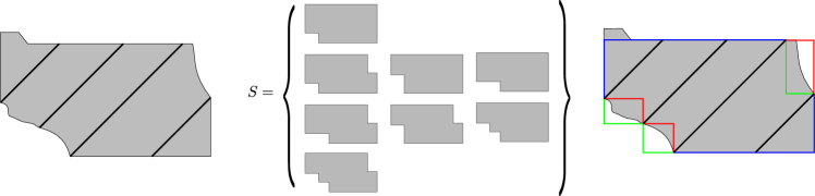
Figure 6: Example of candidates for a $2$-interval module $I$ with support in $\mathbb{R}^{2}$. (Left) Given the $L$-fibered barcode of $I$, where $L$ is the family of the four black lines, we want to approximate $I$ with an element of $S$, i.e., an interval module with the same fibered barcode. (Middle) When one further constrains the set $S$ by asking to have at most one corner between two consecutive endpoints of the fibered barcode, the whole set $S$ can be computed explicitly. (Right) The set $S$ can also be described as the set of intervals which have to go through the blue path, and which can arbitrarily choose between the red or green path at three different locations. Hence, the cardinality of $S$ is $2^{3}$.

For interval modules, $S$ is generally a set of cardinal $c^{d}$, where $c$ is the number of candidate corners between birthpoints or deathpoints, and $d$ is the number of corners. For instance, in Figure 6, one has $n=2$, $c=2$ and $d=3$. Unfortunately, $c$ is of the order of $2^{n-1}$, and thus grows exponentially with the dimension $n$, and $d$ is difficult to control in practice, since it heavily depends on the number of lines in the fibered barcode and the regularity of the underlying interval module $I$. Minimizing a penalty over $S$ is thus practical only for low dimension $n$ and small number of lines in the fibered barcode. Hence, our algorithm MMA presented in Section 4.2 does not use penalty minimization, but is rather defined with natural and simple corner choices.

Remark 4.1.

Note also that there are cases when the corner choices are canonical. For instance, any $2$-multipersistence module $M$ with transition maps $\varphi_{\cdot}^{\cdot}$ that are weakly exact, i.e., that satisfy, for any $x\leq y$

$$\mathrm{im}\left(\varphi_{x}^{y}\right)=\mathrm{im}\left(\varphi_{(y_{1},x_{2})}^{y}\right)\cap\mathrm{im}\left(\varphi_{(x_{1},y_{2})}^{y}\right)\text{ and }\ker\left(\varphi_{x}^{y}\right)=\ker\left(\varphi_{x}^{(y_{1},x_{2})}\right)+\ker\left(\varphi_{x}^{(x_{1},y_{2})}\right),$$

is rectangle decomposable [BLO22]. Hence, a canonical approximation of a summand $I$ of ${\mathbb{M}}$ is given by the interval module whose support is the rectangle with corners $(\min_{l}(b^{I}_{l})_{1},\min_{l}(b^{I}_{l})_{2})$ and $(\max_{l}(b^{I}_{l})_{1},\max_{l}(b^{I}_{l})_{2})$, where $l$ goes through the family of lines $L$ of the fibered barcode.

4.2 MMA algorithm for computing candidate decompositions

In this section, we introduce MMA: a fast algorithm for computing $\delta$-candidate decompositions. The pseudo-code for MMA is provided in Algorithm 1. Roughly speaking, given a multi-parameter persistence module ${\mathbb{M}}$, an approximation parameter $\delta>0$, a $\delta$-grid of lines $L=L_{\delta}(K^{\delta})$ where $K$ contains the multigraded Betti numbers of ${\mathbb{M}}$, and a matching function $\sigma$ that commutes with the exact matching function $\sigma_{\mathbb{M}}$ induced by ${\mathbb{M}}$ (see Section 5 for a discussion about how to find such matching functions), Algorithm 1 works in three steps:

• compute the $L$-fibered barcode of ${\mathbb{M}}$,

• match together bars that correspond to the same underlying summand using the matching function $\sigma$,

• for each summand, use the endpoints of the corresponding bars to compute estimates of the critical points, using Algorithm 2.

Step 1 can be performed using any persistent homology software (such as, e.g., Gudhi, Ripser, Phat, etc), or with Rivet [LW15] when $n=2$. Our code can be found at https://github.com/DavidLapous/multipers, and is based on the vineyard algorithm [CSEM06], which allows us to run Steps 1 and 2 jointly (see Section 5.2).

Input 1: A multi-parameter persistence module ${\mathbb{M}}$ (whose multigraded Betti numbers are included in a hyperrectangle $K$),

Input 2: $\delta$-grid of evenly spaced diagonal lines $L=L_{\delta}(K^{\delta})$

Input 3: Matching function $\sigma$ (commuting with $\sigma_{{\mathbb{M}}}$ if ${\mathbb{M}}$ is interval decomposable)

Output: Candidate decomposition $\tilde{\mathbb{M}}_{\delta}$

Compute ${\mathcal{F}}{\mathcal{B}}({\mathbb{M}})_{L}={\mathcal{F}}{\mathcal{B}}(\mathcal{M})_{L}$, i.e., the $L$-fibered barcode of ${\mathbb{M}}$;

$S\leftarrow$ []; # $S$ is the set of interval summands of the output candidate decomposition, intialized as the empty set

for $l\in L$ do

       for $[b_{l}^{\mathbb{M}},d_{l}^{\mathbb{M}}]\in{\mathcal{B}}({\left.\kern-1.2pt{\mathbb{M}}\vphantom{\big{|}}\right|_{l}})$ do

             # Check whether it is in the image of the input matching

             if $\exists B\in S$ and $[b,d]\in B$ s.t. $[b_{l}^{{\mathbb{M}}},d_{l}^{{\mathbb{M}}}]=\sigma([b,d])$ then

                   $B$.append($[b_{l}^{{\mathbb{M}}},d_{l}^{{\mathbb{M}}}]$); # If it is, attach the bar to the corresponding summand

            # Otherwise initialize a new summand with the bar

             else

                   Add $B:=\{[b_{l}^{\mathbb{M}},d_{l}^{\mathbb{M}}]\}$ to $S$;

# For each summand in $S$ characterized by a set of bars, build an approximate interval summand

Return $\tilde{\mathbb{M}}_{\delta}:=\bigoplus_{B\in S}$ ApproximateInterval$(B)$;

Algorithm 1 MMA: Multi-parameter persistence Module Approximation.

We now describe the algorithm ApproximateInterval, which is used at the end of Algorithm 1. Its pseudo-code is given in Algorithm 2, and is defined in two steps:

1. first, we label birthpoints and deathpoints to identify facets with LabelEndpoints (Algorithm 3),

2. then, we use these labels to compute candidate critical points with ComputeCorners (Algorithm 4).

Input: Set of bars $B=\{[b_{l},d_{l}]\}_{l\in L_{B}}$, where $L_{B}\subseteq L$

Output: Discretely presented interval module $\tilde{I}$

labs $\leftarrow$ LabelEndpoints$(B)$;

$C_{B}^{L}(I),C_{D}^{L}(I)\leftarrow$ ComputeCorners$(B,$ labs$)$;

Return $\tilde{I}(B):=\mathrm{\mathbf{Int}}\left(\bigcup_{c\in C_{B}^{L}(I)}\bigcup_{c^{\prime}\in C_{D}^{L}(I)}R_{c,c^{\prime}}\right)$;

Algorithm 2 ApproximateInterval

We first describe LabelEndpoints. The core idea of this algorithm, whose pseudo-code is given in Algorithm 3, is, for a given bar in $I$ associated to a line $l\in L$, to look at the corresponding surrounding set $L_{l}$. If there exists a hyperplane $H$ such that all endpoints in this surrounding set belong to $H$, we identify $H$ as a facet, and we label the bar with the codirection of $H$.

Input: Set of bars $B=\{[b_{l},d_{l}]\}_{l\in L_{B}}$, where $L_{B}\subseteq L$

Output: List labs of labels for each endpoint in $B$

labs$(b_{l})\leftarrow[]$ for all $l\in L_{B}$;

for $l\in L_{B}$ do

       if $\exists i\in\llbracket 1,n\rrbracket$ and $c_{i}\in\mathbb{R},$ such that $\forall l^{\prime}\in L_{l},\,(b_{l^{\prime}})_{i}=c_{i}$ then

             Add $(i,c_{i})$ to labs$(b_{l^{\prime}})$ for all $l^{\prime}\in L_{l}$;

Return labs;

Algorithm 3 LabelEndpoints

Note that endpoints can have zero or more than one label. For instance, an endpoint that belongs to the intersection of several facets might have multiple labels. However, if several labels are identified, they must be associated to different dimensions. See Figure 7 for examples of label assignments when the underlying interval module has rectangle support.

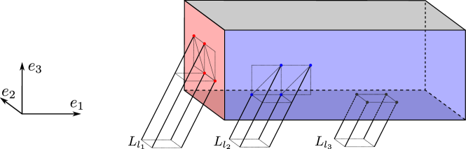
Figure 7: Example of birthpoint labelling for an interval module $I$ with rectangle support with three surrounding sets of lines $L_{l_{1}}$, $L_{l_{2}}$, $L_{l_{3}}$ associated to three lines $l_{1},l_{2},l_{3}$. The labels of $l_{1},l_{2},l_{3}$ that are identified correspond to the red, blue and grey colored facets of $I$ respectively.

Finally, we describe ComputeCorners. The core idea of the algorithm, whose pseudo-code is given in Algorithm 4, is to use the labels identified by LabelEndpoints to compute corners, or critical point estimates, in the following way: if all birthpoints (resp. deathpoints) in a surrounding set have at least one associated facet, i.e., have a non-empty list of labels, then a candidate corner can be defined using the minimum (resp. maximum) of all birthpoints (resp. deathpoints) coordinates. We only present the pseudo-code for birthpoints since the code for deathpoints is symmetric and can be obtained by replacing minimum by maximum and $-\infty$ by $+\infty$.

Input 1: Set of bars $B=\{[b_{l},d_{l}]\}_{l\in L_{B}}$, where $L_{B}\subseteq L$

Input 2: List labs of labels for each endpoint in $B$

Output: List of birth corners $C_{B}$

$C_{B}\leftarrow[]$;

for $l\in L_{B}$ do

       $B_{L_{l}}\leftarrow\{b_{l^{\prime}}:l^{\prime}\in L_{l}\cap L_{B}\}$; # Note that $B_{L_{l}}\subseteq B$ by construction

       # Check whether all birthpoints in the surrounding set belong to $K$

       if  $B_{L_{l}}\subseteq K$ then

             # Compute birth corner if all the birthpoints are labelled

             if labs$(b)\neq\varnothing,\forall b\in B_{L_{l}}$ then

                   $\{(j,c_{j})\,:\,j\in\mathcal{J}\}\leftarrow\bigcup_{b\in B_{L_{l}}}$ labs$(b)$; # $\mathcal{J}\subseteq\llbracket 1,n\rrbracket$ is the set of codirections

                   Define $C^{l}\in\mathbb{R}^{n}$ as

• $(C^{l})_{j}=c_{j}$ if $j\in\mathcal{J}$

• $(C^{l})_{j}=\min{\left\{(b_{l^{\prime}})_{j}\,:\,l^{\prime}\in L_{l}\cap L_{B}\right\}}$ otherwise

$C_{B}$.append$(C^{l})$;

                  

             # If the birthpoints are not all labeled, keep the birthpoints themselves as corners

             else

                   for $l^{\prime}\in L_{l}\cap L_{B}$ do

                        $C_{B}$.append$(b_{l^{\prime}})$;

      # If some birthpoints are not in $K$, they must correspond to infinite facets

       else

             Assert $B_{L_{l}}\cap K^{\delta}\backslash K\neq\varnothing$;

             Assert labs$(b)\neq\varnothing$ for all $b\in B_{L_{l}}$;

             $\{(j,c_{j})\,:\,j\in\mathcal{J}\}\leftarrow\bigcup_{b\in B_{L_{l}}}\textsc{labs}(b)$; # The cardinality of the set of codirections $\mathcal{J}\subsetneq\llbracket 1,n\rrbracket$ must be strictly less than $n$

             Define $C^{l}\in\mathbb{R}^{n}$ as

• $(C^{l})_{j}=c_{j}$ if $j\in\mathcal{J}$

• $(C^{l})_{j}=-\infty$ otherwise

$C_{B}$.append$(C^{l})$;

Return $C_{B}$;

Algorithm 4 ComputeCorners

Complexity.

Computing the $L$-fibered barcode ${\mathcal{F}}{\mathcal{B}}({\mathbb{M}})_{L}$ on a simplicial complex, as well as assigning the corresponding bars to their associated summands in the decomposition of ${\mathbb{M}}$, can be done with the vineyard algorithm and matching [CSEM06] with complexity $O(N^{3}+|L|\cdot N\cdot T)$, where $N$ is the number of simplices in the simplicial complex, and $T$ is the maximal number of transpositions required to update the single-parameter filtrations corresponding to the consecutive lines in $L$. In the worst case scenario, $T=N^{2}$. Note that $T$ usually decreases to a fixed constant as $|L|$ increases, and that this computation can be easily parallelized in practice.

Now, adding the complexities of Algorithms 3 and 4, the final complexity of Algorithm 1 is

$$O(N^{3}+|L|\cdot N\cdot T+|L|\cdot n\cdot 2^{n-1}).$$ (8)

Of importance, the dependence on $n$ is much better than the (exact) decomposition algorithm proposed in [DX22] whose complexity is $O(N^{n(2\omega+1)})$, where $\omega<2.373$ is the matrix multiplication exponent. It is also comparable to Rivet [LW15] (which works only when $n=2$), whose complexity is $O(N^{3}\kappa+(N+{\rm log}\kappa)\kappa^{2})$, where $\kappa=\kappa_{x}\kappa_{y}$ is the product of $x$ and $y$ coordinates used to evaluate the module (note that $\kappa_{x},\kappa_{y}$ are also user-dependent). The elder-rule staircode [CKMW20] works only for point cloud data when $n=2$ and homology dimension $0$, but has better complexity $O(m^{2}\log(m))$, where $m$ is the number of points. Finally, note that our complexity can be controlled by the number of lines, which is user-dependent. We illustrate this useful property in Section 6.

Remark 4.2.

For the sake of simplicity and efficiency, the code that we provide at https://github.com/DavidLapous/multipers contains a simpler version of Algorithm 4, that does not compute and use labels, but rather gathers the birthpoints and deathpoints as corners directly. One can easily check that the correctness result (Proposition 4.3 and its proof below) carries over to that simpler algorithm, however the exactness result (Corollary 4.10 below) is only valid for corners computed with Algorithm 4.

Correctness of MMA.

The following proposition ensures that MMA is correct.

Proposition 4.3.

Let ${\mathbb{M}}$ be an interval decomposable multi-parameter persistence module. Let $\tilde{\mathbb{M}}^{\mathtt{MMA}{}}_{\delta}=\mathtt{MMA}{}({\mathbb{M}},L_{\delta}(K^{\delta}),\sigma)$, where $\sigma$ commutes with $\sigma_{\mathbb{M}}$. Then $\tilde{\mathbb{M}}^{\mathtt{MMA}{}}_{\delta}$ is a $\delta$-candidate decomposition of ${\mathbb{M}}$.

Proof.

Let $I$ be an interval summand of ${\mathbb{M}}$, and $\tilde{I}$ be the associated interval summand of the candidate decomposition $\tilde{\mathbb{M}}^{\mathtt{MMA}{}}_{\delta}$ (which is well-defined as $\sigma$ is assumed to commute with $\sigma_{\mathbb{M}}$). Let $C_{B}^{L}(I)$ and $C_{D}^{L}(I)$ be the birth and death corners computed by Algorithm 4, i.e., one has

$$\tilde{I}=\mathrm{\mathbf{Int}}\left(\bigcup_{c\in C_{B}^{L}(I)}\bigcup_{c^{\prime}\in C_{D}^{L}(I)}R_{c,c^{\prime}}\right),$$ (9)

In order to show that $\tilde{\mathbb{M}}^{\mathtt{MMA}{}}_{\delta}$ is a $\delta$-candidate decomposition of ${\mathbb{M}}$, it suffices to show that the $L$-fibered barcodes of $\tilde{I}$ and $I$ are the same, i.e., ${\mathcal{F}}{\mathcal{B}}(I)_{L}={\mathcal{F}}{\mathcal{B}}(\tilde{I})_{L}$. Equivalently, we need to show that ${\rm supp}(I)\cap l={\rm supp}(\tilde{I})\cap l$ for any line $l\in L$. We first show that they share the same birthpoints, i.e., that $L[I]\cap L=L[\tilde{I}]\cap L$. Let $l\in L$. Note that $b^{I}_{l}$ and $b^{\tilde{I}}_{l}$ are comparable since they belong to the same diagonal line $l$.

Strategy. In order to show $b^{\tilde{I}}_{l}=b^{I}_{l}$, we are going to show that 1. $b^{I}_{l}\leq_{n}b^{\tilde{I}}_{l}$ and 2. $b^{\tilde{I}}_{l}\leq_{n}b^{I}_{l}$.

1. In order to show $b^{I}_{l}\leq_{n}b^{\tilde{I}}_{l}$, we are going to show that $c\not<_{n}b^{I}_{l}$ for any corner $c\in C_{B}^{L}(I)$. Indeed, if one assumes $b^{I}_{l}>_{n}b^{\tilde{I}}_{l}$, and since there always exists a birth corner $c\in C_{B}^{L}(I)$ such that $c\leq_{n}b^{\tilde{I}}_{l}$ by construction of $\tilde{I}$, one has $c\leq_{n}b^{\tilde{I}}_{l}<_{n}b^{I}_{l}$.

2. In order to show $b^{\tilde{I}}_{l}\leq_{n}b^{I}_{l}$, we are going to show that there exists a corner $c\in C_{B}^{L}(I)$ such that $c\leq_{n}b^{I}_{l}$. Indeed, if there is such a birth corner, and if $b^{\tilde{I}}_{l}>_{n}b^{I}_{l}$ by contradiction, then $c\leq_{n}b^{I}_{l}<_{n}b^{\tilde{I}}_{l}$, and $R_{c,b^{\tilde{I}}_{l}}$ is not flat, contradicting Lemma 3.9.

Proof of (2). By construction of $\tilde{I}$ with Algorithm 4, if $b^{I}_{l}$ is labelled, then there exists a line $l^{\prime}$ and a corner $c^{l^{\prime}}\in C_{B}^{L}(I)$ that is smaller than $b^{I}_{l}$ so we can take $c:=c^{l^{\prime}}$. If $b^{I}_{l}$ is not labelled, it belongs itself to $C_{B}^{L}(I)$, and we can take $c:=b^{I}_{l}$.

Proof of (1). Let $c\in C_{B}^{L}(I)$ be a birth corner, and let $L_{l_{0}}$ be the associated surrounding set of lines for some $l_{0}\in L$. Let $[c]_{l}:=\min\left[\left(c+\left(\mathbb{R}_{+}\right)^{n}\right)\cap l\right]$ be the smallest element in the intersection between the positive cone on $c$ and $l$. Assume $[c]_{l}\geq_{n}b^{I}_{l}$ and $c<_{n}b^{I}_{l}$. Then $R_{c,[c]_{l}}$ is not flat, contradicting the fact that $[c]_{l}$ is the smallest element. Thus, we only have to show $[c]_{l}\geq_{n}b^{I}_{l}$. There are two cases.

• Either some birthpoints of $L_{l_{0}}$ are not labelled by Algorithm 3, and $c$ is equal to $b^{I}_{l^{\prime}}$ for some $l^{\prime}\in L_{l_{0}}$. Now, assume $[c]_{l}<_{n}b^{I}_{l}$ by contradiction. Then $b^{I}_{l^{\prime}}=c\leq_{n}[c]_{l}<_{n}b^{I}_{l}$. Thus $b^{I}_{l^{\prime}}<_{n}b^{I}_{l}$ and $R_{b^{I}_{l^{\prime}},b^{I}_{l}}$ is not flat, contradicting Lemma 3.9. Hence $[c]_{l}\geq_{n}b^{I}_{l}$.

• Or all the birthpoints of $L_{l_{0}}$ are labelled by Algorithm 3. Again, we study two separate cases. See Figure 8 for an illustration.

  • Either $l\in L_{l_{0}}$. Then, $\exists i\in\llbracket 1,n\rrbracket$ such that $(b^{I}_{l})_{i}=c_{i}$. This yields $(b^{I}_{l})_{i}=c_{i}\leq([c]_{l})_{i}$, and thus $[c]_{l}\geq_{n}b^{I}_{l}$ since they both belong to the same diagonal line $l$.

  • Or the line $l$ does not belong to $L_{l_{0}}$. Since $[c]_{l}$ is on the boundary of the positive cone based on $c$, there exists $i\in\llbracket 1,n\rrbracket$ such that $([c]_{l})_{i}=c_{i}$. Assume again by contradiction that $b^{I}_{l}>_{n}[c]_{l}$, and write

    $$[c]_{l}=c+\sum_{j\neq i}(\delta\alpha_{j})e_{j}=:c+\overrightarrow{v}<_{n}b^{I}_{l}$$

    with $\alpha_{j}\geq 0$ for $j\in\llbracket 1,n\rrbracket\backslash\left\{i\right\}$. Since $l\notin L_{l_{0}}$, there exists some $j_{0}$ such that $\alpha_{j_{0}}>1$. Let $\overrightarrow{u}:=((\overrightarrow{v}_{j}\,\mathrm{mod}\,\delta)_{j\in\llbracket 1,n\rrbracket})=(([c]_{l}-c)_{j}\,\mathrm{mod}\,\delta)_{j\in\llbracket 1,n\rrbracket}\in[0,\delta)^{n}\leq_{n}\overrightarrow{v}$. Let $l^{\prime}:=l_{c+\overrightarrow{u}}$ be the diagonal line passing through $c+\overrightarrow{u}$. Now, recall that the lines of $L$ are drawn on a grid, so $l^{\prime}\in L$ since $l^{\prime}=l+\overrightarrow{u}-\overrightarrow{v}$. Moreover, one has by definition, $c\in{\rm conv}(L_{l_{0}})$. Since the lines of $L$ are on a grid, one has

    $$\forall l_{1},l_{2}\in L,\|l_{1}\cap H_{n},{\rm conv}(L_{l_{2}})\cap H_{n})\|_{\infty}<\delta\Longrightarrow l_{1}\in L_{l_{2}},\quad$$

    where $H_{n}=\left\{x\in\mathbb{R}^{n}:x_{n}=c_{n}\right\}$. Now, note that $c+\overrightarrow{u}$ and $c+\overrightarrow{u}-\overrightarrow{u}_{n}\cdot\textbf{1}$ both belong to $l^{\prime}$, and that $c+\overrightarrow{u}-\overrightarrow{u}_{n}\cdot\textbf{1}\in H_{n}$. Moreover, since

    $$\left\lVert(c+(\overrightarrow{u}-\overrightarrow{u}_{n}\cdot\textbf{1}))-c\right\rVert_{\infty}=\left\lVert\overrightarrow{u}-\overrightarrow{u}_{n}\cdot\textbf{1}\right\rVert_{\infty}<\delta,$$

    one has $l^{\prime}\in L_{l_{0}}$. Thus, there exists $i^{\prime}\in\llbracket 1,n\rrbracket$ such that $(b^{I}_{l^{\prime}})_{i^{\prime}}=c_{i^{\prime}}\leq(c+\overrightarrow{u})_{i^{\prime}}$ and thus $b^{I}_{l^{\prime}}\leq_{n}(c+\overrightarrow{u})$ since $b^{I}_{l^{\prime}}$ and $c+\overrightarrow{u}$ are comparable on the diagonal line $l^{\prime}$. Finally, $b^{I}_{l^{\prime}}\leq_{n}c+\overrightarrow{u}\leq_{n}c+\overrightarrow{v}<_{n}b^{I}_{l}$, and $R_{b^{I}_{l^{\prime}},b^{I}_{l}}$ is not flat, contradicting Lemma 3.9. Hence, $b^{I}_{l}\leq_{n}[c]_{l}$.

  

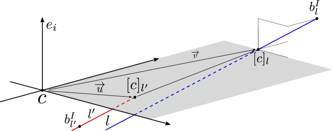
  Figure 8: Illustration of $l,l^{\prime},c,[c]_{l},[c]_{l^{\prime}},\overrightarrow{u},\overrightarrow{v},b^{I}_{l},b^{I}_{l^{\prime}}$ when one assumes that $[c]_{l}<_{n}b^{I}_{l}$.

The proof applies straightforwardly to deathpoints by symmetry. ∎

In order for Proposition 4.3 to apply, one needs to find a matching function $\sigma$ that commutes with the one induced by the underlying module ${\mathbb{M}}$. In practice, partial matchings induced by bottleneck or Wasserstein distances do not work (see Section 5). Instead, one can use the matching $\sigma_{\rm vine}$ induced by the vineyards algorithm [CSEM06]—we show in Section 5.2 that this matching commutes with $\sigma_{\mathbb{M}}$ when the (single-parameter) filtrations induced by lines that are consecutive in $L$ differ by at most one transposition. This can be guaranteed by choosing $\delta$ to be sufficiently small.

4.3 Exact reconstruction with MMA

In this section, we identify the interval decomposable multi-parameter persistence modules that can be recovered exactly with MMA. Given a size parameter $\delta>0$, they correspond to modules that can decomposed into interval summands that form a subclass of the family of discretely presented interval modules, that we call the $\delta$-discretely presented interval modules.

Definition 4.4 ($\delta$-discretely presented interval module).

Let $K\subseteq\mathbb{R}^{n}$ be a hyperrectangle of $\mathbb{R}^{n}$, and let $I$ be a discretely presented interval module. Given $\delta>0$, we say that $I$ is $\delta$-discretely presented in $K$ if:

1. (Large facets) for each point $x\in L[I]$ (resp. $U[I]$) there exists, for each facet $F$ containing $x$, an $(n-1)$-hypercube $Q^{x}_{F}$ of side length $2\delta$ such that $x\in Q^{x}_{F}$ and $Q^{x}_{F}\subseteq F$;

2. (Large holes) if there exists a diagonal line $l$ such that $l\cap{\rm supp}(I)=\varnothing$, then there exists an $n$-hypercube $R$ of side length $\delta$ containing ${\bf 0}$ such that for any line $l^{\prime}$ in $l+R$, one has $l^{\prime}\cap{\rm supp}(I)=\varnothing$;

3. (Locally small complexity) any $\infty$-ball of radius $\delta$, i.e., any set $B_{\delta}(x):=\{y\in\mathbb{R}^{n}:d_{\infty}(x,y)\leq\delta\}$ for some $x\in\mathbb{R}^{n}$, intersects at most one facet in $L[I]$ (resp. $U[I]$) of any fixed codirection;

4. (Compact description) each facet of $I$ has a non-empty intersection with $K$.

Assumptions 1 and 2 ensures that the pieces of ${\rm supp}(I)$ are large enough w.r.t. $\delta$, while Assumptions 3 and 4 ensure that surrounding sets of lines can detect at most one facet associated to a given codirection at a time, and that critical points of $I$ are all included in the hyperrectangle $K$ respectively.

Remark 4.5.

One might wonder whether Assumption 2 and Assumption 3 are redundant with Assumption 1. In other words, one might wonder whether it is actually possible to define an interval module with large facets and small holes, or with large facets that can share the same codirection and lie close to each other at the same time. Even though this seems to be impossible when $n=2$ (indicating that Assumption 2 and Assumption 3 might indeed be redundant with Assumption 1), it can happen when $n\geq 3$, as Figure 9 shows.

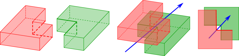
Figure 9: Example of interval module in dimension $n=3$ with large facets, small holes and some facets with the same codirection close to each other. The support of the module can be constructed by taking the (closed) red and (open) green $L$-shaped sets on (Left), and glue them together as shown in (Middle). While arbitrarily large facets can be created using this construction, the resulting interval always contains a small hole and large facets of same codirection that are close to each other. Because of this, it is possible to find a (blue) diagonal line that goes through the support without intersecting it, while lines in its surrounding set will detect some facets. (Right) View of the interval from the top showing the hole and the spatially close facets (showed in bold font). This is an example where Assumptions 1 and 4 of Definition 4.4 are satisfied, while Assumptions 2 and 3 are not.

The main advantage of $\delta$-discretely presented modules is that they ensure that Algorithm 3 can identify every single facet with a corresponding label.

Lemma 4.6.

Let $\delta>0$ and $K$ be a hyperrectangle of $\mathbb{R}^{n}$. Let $I$ be a $\delta$-discretely presented interval module in $K$, and let $L$ be the $\delta$-grid of lines associated to $K^{2\delta}$. Then, there is a bijection between the facets of $I$ and the labels identified by Algorithm 3.

Proof.

We first prove the result for birthpoints and facets of $L[I]$.

Let $F$ be a facet of $L[I]$. Let $l_{F}\in L$ be a diagonal line intersecting $F$, and $b_{F}\in\mathbb{R}^{n}$ be the associated birthpoint. By Definition 4.4, item (1), there exists an $(n-1)$-hypercube $Q_{F}^{b_{F}}\subseteq F$ of side length $2\delta$ such that $b_{F}\in Q_{F}^{b_{F}}$. This ensures that for any dimension $i$ that is not in the codirection: $i\in\llbracket 1,n\rrbracket\backslash{\rm codir}(F)$, one has either $b_{F}+\delta e_{i}\in Q_{F}^{b_{F}}$ or $b_{F}-\delta e_{i}\in Q_{F}^{b_{F}}$. Since $L$ is the $\delta$-grid of lines associated to $K^{2\delta}$, and since $Q_{F}^{b_{F}}$ is an $(n-1)$-hypercube, there exists a line $l_{0}\in L$ such that $l_{F}$ belongs to the surrounding set $L_{l_{0}}$, and such that the birthpoints corresponding to the lines in $L_{l_{0}}$ are all in $Q_{F}^{b_{F}}$. This means that ${\rm codir}(F)$ is detected as a label of $b_{F}$ by Algorithm 3.

Reciprocally, assume there exists a line $l_{0}\in L$ such that all birthpoints associated to the lines in the surrounding set $L_{l_{0}}$ share a coordinate along dimension $i\in\llbracket 1,n\rrbracket$, so that $i$ is a label detected by Algorithm 3. Then, the set of birthpoints $B_{L_{l_{0}}}$ has a minimal element, and thus its convex hull ${\rm conv}(B_{L_{l_{0}}})$ is in $L[I]$. Since ${\rm conv}(B_{L_{l_{0}}})$ is an $(n-1)$-hypercube of codirection $i$, it must be associated to a facet of $L[I]$ of codirection $i$ as well.

The proof extends straightforwardly for deathpoints. ∎

Now that we have proved that all facets can be detected with $\delta$-grids of lines and $\delta$-discretely presented modules, we can state our first main result, which claims that it is possible to exactly recover the underlying module under the same assumptions.

Proposition 4.7 (Exact recovery).

Let $\delta>0$ and $K=R_{\alpha,\beta}$ be a hyperrectangle of $\mathbb{R}^{n}$, where $\alpha\leq_{n}\beta$. Let $I$ be a $\delta$-discretely presented interval module in $K$, and let $L$ be the $\delta$-grid of lines associated to $K^{2\delta}$. Let $C_{B}^{L}(I)$ and $C_{D}^{L}(I)$ be the $L$-birth and death corners of $I$ computed by Algorithm 4, and let $\tilde{I}=\mathrm{\mathbf{Int}}\left(\bigcup_{c\in C_{B}^{L}(I)}\bigcup_{c^{\prime}\in C_{D}^{L}(I)}R_{c,c^{\prime}}\right)$ be the approximation computed by Algorithm 2. Then, one has

$${d_{\rm I}}(I,\tilde{I})={d_{\rm B}}(I,\tilde{I})=0.$$ (10)

Proof.

As interval modules are characterized by their support, it is enough to show that $\overline{{\rm supp}(I)}=\overline{{\rm supp}(\tilde{I})}$. In the following, we thus assume that ${\rm supp}(I)$ is closed in $\overline{\mathbb{R}}^{n}$. We will also use an additional definition. Let $b$ be an infinite corner computed by Algorithm 4. We say that $b^{\prime}$ is a pseudo birth corner for $b$ if:

1. $b^{\prime}_{i}=b_{i}$ for all $i\in\llbracket 1,n\rrbracket\backslash\mathcal{J}$, and for each dimension $j\in\mathcal{J}$, there exists a hyperplane of codirection $j$ intersecting $K$ such that $\bigcap_{j}H_{j}\ni b^{\prime}$. The set $\mathcal{J}$ is called the codirection of $b^{\prime}$ and denoted with ${\rm codir}(b^{\prime})$, and the set $\llbracket 1,n\rrbracket\backslash\mathcal{J}$ is called the direction of $b^{\prime}$ and is denoted with ${\rm dir}(b^{\prime})$.

2. there exists a line $l_{0}\in L$ such that

   1. $b^{\prime}\in{\rm conv}(L_{l_{0}})\cap K^{2\delta}\backslash K$,

   2. for each line $l\in L_{l_{0}}$, the endpoint $b_{l}^{I}$ is non trivial,

   3. for each dimension $j\in\mathcal{J}$, there exists $l_{j}\in L_{l_{0}}$ such that $b_{l_{j}}^{I}\in H_{j}$.

Note that codirections can be extended to any finite corner (i.e., that is potentially not the pseudo corner of an infinite corner) straightforwardly, and that pseudo death corners can be defined by symmetry. We now prove Proposition 4.7.

We first show the inclusion ${\rm supp}(\tilde{I})\subseteq{\rm supp}(I)$. More specifically, we have to prove that the corners computed by Algorithm 4 all belong to ${\rm supp}(I)$. A key argument that we will use several times comes from the following lemma, which allows for a local control of the boundary of ${\rm supp}(I)$ using the hyperplanes associated to specific corners.

Lemma 4.8.

Let $b$ be a birthpoint (resp. deathpoint) of $I$ in $K^{\delta}$, and $l_{0}\in L$ be the line such that $b\in{\rm conv}(L_{l_{0}})$ (this line exists since $L$ fills $K^{\delta}$). Then, one has the following:

1. for any facet $F$ of $L[I]$ (resp. $U[I]$) containing $b$, there exists a line $l_{F}\in L_{l_{0}}$ such that $b_{l_{F}}^{I}\in F$ (resp. $d_{l_{F}}^{I}\in F$).

2. for any dimension $i$, there exists at most one facet of codirection $i$ intersecting the set of birthpoints (resp. deathpoints) $\left\{b_{l}^{I}:l\in L_{l_{0}}\right\}$ (resp. $\left\{d_{l}^{I}:l\in L_{l_{0}}\right\}$.

3. let $b^{\prime}_{L_{l_{0}}}$ (resp. $d^{\prime}_{L_{l_{0}}}$) be the finite corner generated by $L_{l_{0}}$. Then, one has:

   $${\rm conv}(L_{l_{0}})\cap L[I]\cap K^{2\delta}\subseteq\bigcup_{i\in{\rm codir}(b^{\prime})}\left\{x\in\mathbb{R}^{n}:x_{i}=b^{\prime}_{i}\right\}$$

   (resp. $${\rm conv}(L_{l_{0}})\cap U[I]\cap K^{2\delta}\subseteq\bigcup_{i\in{\rm codir}(d^{\prime})}\left\{x\in\mathbb{R}^{n}:x_{i}=d^{\prime}_{i}\right\}\text{)}.$$

Proof.

We only show the result for birthpoints since the arguments for deathpoints are the same. Let $b\in L[I]$ be a birthpoint in $K^{\delta}$.

Proof of (1). Let $F$ be a facet containing $b$. According to Definition 4.4, item (1), there exists an $(n-1)$-hypercube $Q^{b}_{F}$ of side length $2\delta$ such that $Q^{b}_{F}\subseteq F$ and $b\in Q^{b}_{F}$. Since $L$ is a grid, there exists a line $l\in L$ with $d_{\infty}(b,l)<\delta$ intersecting $Q^{b}_{F}$. Now, since $b\in{\rm conv}(L_{l_{0}})$, one has $d_{\infty}(l\cap H_{F},L_{l_{0}}\cap H_{F})<\delta$, where $H_{F}$ is the hyperplane containing $F$; thus, $l\in L_{l_{0}}$ (the argument is the same than in the proof of Proposition 3.13, first paragraph).

Proof of (2). By Proposition 3.13, item (2), the birthpoints associated to lines of $L_{l_{0}}$ are all contained in a ball of radius $\delta$. Thus, the unicity of the facets with given codirection comes straightforwardly from Definition 4.4, item (3).

Proof of (3). Note that the birthpoint $b$ is obviously included in the facets of $L[I]$ that contain it, which is a subset of the facets associated to the birthpoints of the lines in $L_{l_{0}}$. Now, as Lemma 4.6 ensures that the birthpoints associated to lines in $L_{l_{0}}$ are correctly labelled, the corner generated by $L_{l_{0}}$ must be on the intersection of the facets containing $b$. This ensures that

$$b\in\bigcup_{i\in\mathrm{codir}(b^{\prime})}\left\{x\in\mathbb{R}^{n}:x_{i}=b^{\prime}_{i}\right\}.$$

Since these arguments do not depend on $b\in{\rm conv}(L_{l_{0}})$, the result follows. ∎

Now that we have Lemma 4.8, we can prove that finite and infinite corners belong to ${\rm supp}(I)$. We will prove the results for birth corners, but the arguments for death corners are symmetric.

Finite corners. Let $b$ be a finite birth corner, associated to a set of consecutive lines $L_{l_{0}}$ for some line $l_{0}\in L$. By assumption, each birthpoint $b_{l}^{I}$, for $l\in L_{l_{0}}$, is nontrivial; and thus any birthpoint in ${\rm conv}(L_{l_{0}})$ is nontrivial as well, using Definition 4.4, item (2). Let $l\in{\rm conv}(L_{l_{0}})$ be the diagonal line passing through $b$.
Using Lemma 4.8, one has:

$$b_{l}^{I}\in{\rm conv}(L_{l_{0}})\cap L[I]\cap K^{2\delta}\subseteq\left(\bigcup_{i\in{\rm codir}(b)}\left\{x\in\mathbb{R}^{n}:x_{i}=b_{i}\right\}\right)\cap l=\left\{b\right\}.$$

Thus $b=b_{l}^{I}$ and $b\in{\rm supp}(I)$.

Infinite corners. Let $b$ be an infinite birth corner, and let $b^{\prime}$ be the minimal (w.r.t. $\leq_{n}$) pseudo birth corner for $b$, which is well defined by construction of $b$ (see Algorithm 4). Let $L_{l_{0}}$ be the associated set of consecutive lines $L_{l_{0}}$, for some line $l_{0}\in L$. We will show that, if $j$ is a free coordinate of $b^{\prime}$, i.e., if $j\in{\rm dir}(b^{\prime})$, then $b^{\prime}_{j}<\alpha_{j}$ (recall that $K$ is the rectangle $R_{\alpha,\beta}$). The reason we want to prove such inequalities is that they directly lead to the result. Indeed, if $b^{\prime}_{j}<\alpha_{j}$ for any $j\in{\rm dir}(b^{\prime})$, then $b^{\prime}-t\sum_{j\in{\rm dir}(b^{\prime})}e_{j}$ belongs to $L[I]$ for any $t>0$, since otherwise the line $\{b^{\prime}-t\sum_{j\in{\rm dir}(b^{\prime})}e_{j}:t>0\}$ would have to intersect a facet $F\subseteq L[I]$ of codirection $j$ for some $j\in{\rm dir}(b^{\prime})$, which would not intersect $K$, contradicting Definition 4.4, item (4).

Let $j\in{\rm dir}(b^{\prime})$ be a free coordinate. By contradiction, assume that $b^{\prime}_{j}\geq\alpha_{j}$, and let $b^{j}$ denote the pseudo birth corner generated by $L_{l_{0}-\delta e_{j}}$. In particular, this means that, for any $l\in L_{l_{0}}$, $l-\delta e_{j}\in L$ and $L_{l-\delta e_{j}}\subseteq L$ since $L$ fills $K^{\delta}$. Now, if for every line $l\in L_{l_{0}}$ such that $l=l_{0}+\overrightarrow{v}$ with $\overrightarrow{v}_{j}=0$, one has that $b_{l}^{I}$ and $b_{l-\delta e_{j}}^{I}$ are on the same facets, then one has $b_{l-\delta e_{j}}^{I}=b_{l}^{I}-\delta e_{j}$, and the pseudo corner $b^{j}$ is equal to $b^{\prime}-\delta e_{j}$ by construction, as per Algorithm 4. Moreover, one has $b^{j}=b^{\prime}-\delta e_{j}\leq_{n}b^{\prime}$, contradicting the fact that $b^{\prime}$ is minimal. Hence, there is at least one line $l\in L_{l_{0}}$, $l=l_{0}+\overrightarrow{v}$ with $\overrightarrow{v}_{j}=0$, such that $b_{l}^{I}$ and $b_{l-\delta e_{j}}^{I}$ are not on the same facets, in other words, there exists a facet $F_{j}$ of $L[I]$ of codirection $j$ that intersects the (half-open) segment $[b_{l}^{I}-\delta e_{j},b_{l}^{I})$. In order to locate that facet more precisely, we will prove the following lemma:

Lemma 4.9.

For any $i\in\llbracket 1,n\rrbracket$ and $s,t\in\mathbb{R}$ such that $s<t$, one has $(b^{I}_{l-te_{i}})_{i}\leq(b^{I}_{l-se_{i}})_{i}$.

Proof.

Without loss of generality, assume $s=0$. Since $b^{I}_{l}-te_{i}\in l-te_{i}$, it follows that $b^{I}_{l}-te_{i}$ and $b^{I}_{l-te_{i}}$ are comparable. Moreover, one must have $b^{I}_{l}-te_{i}\leq_{n}b^{I}_{l-te_{i}}$, otherwise one would have $b^{I}_{l}>_{n}b^{I}_{l}-te_{i}>_{n}b^{I}_{l-te_{i}}$, contradicting Lemma 3.9. If the points are equal, i.e., $b^{I}_{l}-te_{i}=b^{I}_{l-te_{i}}$, then one has $(b^{I}_{l})_{i}\geq(b^{I}_{l-te_{i}})_{i}$. Otherwise, if $b^{I}_{l}-te_{i}<_{n}b^{I}_{l-te_{i}}$, then

$$\forall k\neq i,\,(b^{I}_{l-te_{i}})_{k}>(b^{I}_{l})_{k}.$$

Moreover, since $b^{I}_{l}$ and $b^{I}_{l-te_{i}}$ cannot be comparable as per Lemma 3.9 one must have $(b^{I}_{l-te_{i}})_{i}\leq(b^{I}_{l})_{i}$.

∎

Let $H_{j}=\left\{x\in\mathbb{R}^{n}:x_{j}=c_{j}\right\}$ be the hyperplane associated to $F_{j}$. Then, by Lemma 4.9, one has

$$(b_{l-\delta e_{j}}^{I})_{j}\leq c_{j}<(b_{l}^{I})_{j}.$$

Since the lines $l$ and $l-\delta e_{j}$ both belong to the surrounding set $L_{l_{0}-\delta e_{j}}$, it follows from Lemmas 4.6, and 4.8, item (3), that ${\rm codir}(b^{j})\supseteq{\rm codir}(b^{\prime})\cup\left\{j\right\}$. Moreover, since the facets of $L[I]$ associated to ${\rm codir}(b^{j})$ are unique in a $\delta$-ball around $b^{j}$, as per Definition 4.4, item (3), they all have a unique associated value $c_{i}$ (corresponding to their associated hyperplanes).

Finally, we will show that $b^{j}\leq_{n}b^{\prime}$. Let $i\in\llbracket 1,n\rrbracket$ be an arbitrary dimension.

• If $i\in{\rm codir}(b^{\prime})$, then $b^{j}_{i}=b^{\prime}_{i}$.

• If $i\in{\rm codir}(b^{j})\backslash{\rm codir}(b^{\prime})$, then $b^{j}_{i}\in\left\{c_{i},\min_{l\in L_{l_{0}-\delta e_{j}}}(b_{l}^{I})_{i}\right\}\leq\min_{l\in L_{l_{0}}}(b_{l}^{I})_{i}=b^{\prime}_{i}$, with a strict inequality for $i=j$.

• If $i\in{\rm dir}(b^{j})\subseteq{\rm dir}(b^{\prime})$, then $b^{j}_{i}=\min_{l\in L_{l_{0}-\delta e_{j}}}(b_{l}^{I})_{i}\leq\min_{l\in L_{l_{0}}}(b_{l}^{I})_{i}=b^{\prime}_{i}$.

Hence, one always has $b^{j}_{i}\leq b^{\prime}_{i}$, and thus $b^{j}<_{n}b^{\prime}$, which contradicts the fact that $b^{\prime}$ is minimal. Thus, one must have $b^{\prime}_{j}<\alpha_{j}$.

We now show that ${\rm supp}(I)\subseteq{\rm supp}(\tilde{I})$. Let $x\in{\rm supp}(I)$. We will show that there exists a birth corner $c$ such that $c\leq_{n}x$. Let $\mathcal{H}$ be the family of hyperplanes associated to the facets of $L[I]$. The corner $c$ will be defined as the limit of a sequence of points $\{x^{(k)}\}_{k\in\mathbb{N}^{*}}$in $\overline{\mathbb{R}}^{n}$, defined by induction with:

1. $x^{(1)}=\inf\left\{x-t\cdot\mathbf{1}:t\geq 0\right\}\cap{\rm supp}(I)$. Then, one has the two following possibilities:

   • either $x^{(1)}=-\boldsymbol{\infty}$, and we let $c:=x^{(1)}$.

   • or there exists a maximal subset of hyperplanes $\mathcal{H}^{1}\subset\mathcal{H}$, $\mathcal{H}^{1}\neq\varnothing$, such that $x^{(1)}\in\cap_{H\in\mathcal{H}^{1}}H=:H_{1}$. Let $\mathcal{J}^{1}\subseteq\llbracket 1,n\rrbracket$ be the set of free coordinates in $H_{1}$, i.e., those dimensions such that $j\in\mathcal{J}^{1}\Longleftrightarrow x^{(1)}-e_{j}\in H_{1}$.

2. $x^{(2)}=\inf\left\{x^{(1)}-t\cdot\sum_{j\in\mathcal{J}^{1}}e_{j}:t\geq 0\right\}\cap{\rm supp}(I)$. Then, one has the two following possibilities:

   • either $x^{(2)}$ is at infinity in $H_{1}$, i.e., $x^{(2)}_{j}=-\infty$ if $j\in\mathcal{J}^{1}$ and $x^{(2)}_{j}=x^{(1)}_{j}$ otherwise, and we let $c:=x^{(2)}$.

   • or there exists a maximal subset of hyperplanes $\mathcal{H}^{2}\supsetneq\mathcal{H}^{1}$ such that $x^{(2)}\in\cap_{H\in\mathcal{H}^{2}}H=:H_{2}$. Let $\mathcal{J}^{2}\subseteq\llbracket 1,n\rrbracket$ be the set of free coordinates in $H_{2}$, i.e., those dimensions such that $j\in\mathcal{J}^{2}\Longleftrightarrow x^{(2)}-e_{j}\in H_{2}$.

3. For $k\geq 3$, $x^{(k+1)}=\inf\left\{x^{(k)}-t\cdot\sum_{j\in\mathcal{J}^{k}}e_{j}:t\geq 0\right\}\cap{\rm supp}(I)$. Then, one has the two following possibilities:

   • either $x^{(k+1)}$ is at infinity in $H_{k}$, i.e., $x^{(k+1)}_{j}=-\infty$ if $j\in\mathcal{J}^{k}$ and $x^{(k+1)}_{j}=x^{(k)}_{j}$ otherwise, and we let $c:=x^{(k+1)}$.

   • or there exists a maximal subset of hyperplanes $\mathcal{H}^{k+1}\supsetneq\mathcal{H}^{k}$ such that $x^{(k+1)}\in\cap_{H\in\mathcal{H}^{k+1}}H=:H_{k+1}$. Let $\mathcal{J}^{k+1}\subseteq\llbracket 1,n\rrbracket$ be the set of free coordinates in $H_{k+1}$, i.e., those dimensions such that $j\in\mathcal{J}^{k+1}\Longleftrightarrow x^{(k+1)}-e_{j}\in H_{k+1}$.

If this sequence stops at step one, i.e., $c=x^{(1)}=-\boldsymbol{\infty}$, then every birthpoint of $I$ is at $-\boldsymbol{\infty}$, the only birth corner is $c=-\boldsymbol{\infty}$, and one trivially has $c\leq_{n}x$. Hence, we assume in the following that $c$ is obtained after at least one iteration of the sequence. Note that this sequence of points has length at most $n$. Let $c^{-}$ and $c$ be the penultimate and last elements of the sequence respectively, and let $\mathcal{J}^{-}$ be the set of free coordinates associated to $c^{-}$. By construction, one has:

$$c\leq_{n}c^{-}\leq_{n}\cdots\leq_{n}x^{(2)}\leq_{n}x^{(1)}\leq_{n}x.$$

We now show that $c$ is indeed a birth corner. If $c$ is finite, then it must belong to the intersection of $n$ hyperplanes, and it is thus a finite birth corner. Hence, we assume now that $c$ is not finite. We will construct a minimal pseudo birth corner from $c^{-}$, and show that $c$ is its associated infinite birth corner. We will consider two different cases, depending on whether $c^{-}$ is close to $K=R_{\alpha,\beta}$ or not. If $c^{-}\in K^{\delta}$, the filling property of $L$ and the size of the facets of $L[I]$ ensure that $c^{-}$ is itself a minimal pseudo birth corner, associated to $c$, which is thus an infinite birth corner. If $c^{-}\notin K^{\delta}$, then let $\overrightarrow{v}\in\mathbb{R}^{n}$ be a vector that pushes back $c^{-}$ into $K^{\delta}$, i.e., such that, for any dimension $i\in\mathcal{J}^{-}$, one has

$$\alpha_{i}-\delta\leq(c^{-}+\overrightarrow{v})_{i}<\alpha_{i},$$

and $\overrightarrow{v}_{i}=0$ if $i\notin\mathcal{J}^{-}$. Let $S$ be the segment $[c^{-},c^{-}+\overrightarrow{v}]$. We have the two following cases:

1. Assume $S\subseteq L[I]$. Then $c^{-}+\overrightarrow{v}\in{\rm supp}(I)\cap K^{\delta}$, and there exists a line $l\in L$ such that $c^{-}+\overrightarrow{v}\in{\rm conv}(L_{l})$. Let $c^{l}$ be the pseudo birth corner associated to $L_{l}$. Since one has $c^{l}_{j}<\alpha_{j}$ for any dimension $j\in\mathcal{J}^{-}$, it follows that $\mathcal{J}^{-}\subseteq{\rm dir}(c^{l})$. Furthermore, since $c^{-}+\overrightarrow{v}$ belongs to the same facets than $c$ and $c^{-}$, and since $c^{-}+\overrightarrow{v}\in{\rm conv}(L_{l})$ one has ${\rm codir}(c^{l})\supseteq{\rm codir}(c)$ and ${\rm dir}(c)=\mathcal{J}^{-}$. Thus, $c$ is an infinite birth corner associated to the minimal pseudo birth corner $c^{l}$.

2. Assume $S\not\subseteq L[I]$. In that case, there must be a facet of codirection $j$, for some $j\in\mathcal{J}^{-}$, that intersects $S$. Since one has $c^{-}_{j}\leq(c^{-}+\overrightarrow{v})_{j}<\alpha_{j}$ for any $j\in\mathcal{J}^{-}$, this means that the facet would not intersect $K$, which yields to a contradiction as per Definition 4.4, item (4).

This concludes that ${\rm supp}(I)\subseteq{\rm supp}(\tilde{I})$, and the equality between these supports holds. ∎

Proposition 4.7 extends to the following corollary, whose proof is immediate from the definition of exact matchings (see Definition 3.1 above).

Corollary 4.10.

Let ${\mathbb{M}}$ be an interval decomposable multi-parameter persistence module, whose interval summands all satisfy the assumptions of Proposition 4.7. Let $\tilde{\mathbb{M}}^{\mathtt{MMA}{}}_{\delta}:=\mathtt{MMA}({\mathbb{M}},L_{\delta}(K^{2\delta}),\sigma)$ be the multi-parameter persistence module computed by $\mathtt{MMA}{}$. Then, one has

$${d_{\rm I}}({\mathbb{M}},\tilde{\mathbb{M}}^{\mathtt{MMA}{}}_{\delta})={d_{\rm B}}({\mathbb{M}},\tilde{\mathbb{M}}^{\mathtt{MMA}{}}_{\delta})=0.$$

4.4 Stability properties of MMA

In the previous sections, we have seen that MMA provides candidate decompositions that approximate well, and sometimes exactly, the interval decomposition of the true underlying module, when it exists. In this section, we focus on the general case, when ${\mathbb{M}}$ does not decompose into simple summands, so that there is no clear notion of induced matching $\sigma_{\mathbb{M}}$. In this case, using matching functions that pair bars that are compatible still preserves structural properties of ${\mathbb{M}}$ with MMA. Thus we start by defining compatibility.

Definition 4.11 (Compatible bars).

Let ${\mathbb{M}}$ be a multi-parameter persistence module, and let $l_{1},l_{2}\subseteq\mathbb{R}^{n}$ be two diagonal lines that are at distance $\delta$ from each other. Assume ${\rm supp}({\mathbb{M}})\cap l_{1}$ and ${\rm supp}({\mathbb{M}})\cap l_{2}$ are not empty, and let $[b^{\mathbb{M}}_{l_{1}},d^{\mathbb{M}}_{l_{1}}]$ and $[b^{\mathbb{M}}_{l_{2}},d^{\mathbb{M}}_{l_{2}}]$ be bars in ${\mathcal{B}}({\left.\kern-1.2pt{\mathbb{M}}\vphantom{\big{|}}\right|_{l_{1}}})$ and ${\mathcal{B}}({\left.\kern-1.2pt{\mathbb{M}}\vphantom{\big{|}}\right|_{l_{2}}})$, characterized by their endpoints. These bars are compatible if the rectangles $R_{b^{\mathbb{M}}_{l_{1}},b^{\mathbb{M}}_{l_{2}}}$, $R_{b^{\mathbb{M}}_{l_{2}},b^{\mathbb{M}}_{l_{1}}}$, $R_{d^{\mathbb{M}}_{l_{1}},d^{\mathbb{M}}_{l_{2}}}$ and $R_{d^{\mathbb{M}}_{l_{2}},d^{\mathbb{M}}_{l_{1}}}$ are flat. Moreover, we say that $[b^{\mathbb{M}}_{l_{1}},d^{\mathbb{M}}_{l_{1}}]$ is compatible with the empty set in $l_{2}$ if $\left\lVert b^{\mathbb{M}}_{l_{1}}-d^{\mathbb{M}}_{l_{1}}\right\rVert_{\infty}\leq 2\delta$.

A compatible matching function is a matching function that only pairs bars that are compatible.

Note that the vineyards algorithm provides compatible matching functions when $\delta$ is small enough (see Section 5.2). The main motivation for using compatible matching functions is that the candidate decompositions they induce with MMA preserve the barcodes on any diagonal line intersecting $K$ up to $2\delta$.

Proposition 4.12.

Let ${\mathbb{M}}$ be a multi-parameter persistence module. Let $\sigma$ be a compatible matching function for ${\mathcal{F}}{\mathcal{B}}({\mathbb{M}})_{L}$, and let $\tilde{\mathbb{M}}^{\mathtt{MMA}{}}_{\delta}:=\mathtt{MMA}({\mathbb{M}},L_{\delta}(K^{\delta}),\sigma)$. Let $l$ be a diagonal line intersecting $K$. Then, one has ${d_{\rm B}}({\mathcal{B}}({\left.\kern-1.2pt{\mathbb{M}}\vphantom{\big{|}}\right|_{l}}),{\mathcal{B}}({\left.\kern-1.2pt\tilde{\mathbb{M}}\vphantom{\big{|}}\right|_{l}}))=0$ if $l\in L$, and ${d_{\rm B}}({\mathcal{B}}({\left.\kern-1.2pt{\mathbb{M}}\vphantom{\big{|}}\right|_{l}}),{\mathcal{B}}({\left.\kern-1.2pt\tilde{\mathbb{M}}\vphantom{\big{|}}\right|_{l}}))\leq 2\delta$ otherwise.

Proof.

Since the proof of Proposition 4.3 above is based on repeated applications of Lemma 3.9, the exact same arguments can be used to prove the first part of Proposition 4.12 (the fact that MMA with compatible matchings provides $\delta$-candidate decompositions, i.e., preserve exactly the $L$-fibered barcodes). Indeed, compatible matchings also guarantee (by definition) the flatness of rectangles created by consecutive endpoints. The general upper bound for any diagonal line is then a simple consequence of Lemma 3.10. Indeed, given a line $l\not\in L$, there must be a line $l^{*}\in L$ such that $l^{*}=l+\overrightarrow{u}$ with $\left\lVert\overrightarrow{u}\right\rVert\leq\delta$ since $L$ fills $K$. Then, one has ${d_{\rm B}}({\mathcal{B}}({\left.\kern-1.2pt{\mathbb{M}}\vphantom{\big{|}}\right|_{l}}),{\mathcal{B}}({\left.\kern-1.2pt\tilde{\mathbb{M}}\vphantom{\big{|}}\right|_{l}}))\leq{d_{\rm B}}({\mathcal{B}}({\left.\kern-1.2pt{\mathbb{M}}\vphantom{\big{|}}\right|_{l}}),{\mathcal{B}}({\left.\kern-1.2pt{\mathbb{M}}\vphantom{\big{|}}\right|_{l^{*}}}))+{d_{\rm B}}({\mathcal{B}}({\left.\kern-1.2pt{\mathbb{M}}\vphantom{\big{|}}\right|_{l^{*}}}),{\mathcal{B}}({\left.\kern-1.2pt\tilde{\mathbb{M}}\vphantom{\big{|}}\right|_{l^{*}}}))+{d_{\rm B}}({\mathcal{B}}({\left.\kern-1.2pt\tilde{\mathbb{M}}\vphantom{\big{|}}\right|_{l^{*}}}),{\mathcal{B}}({\left.\kern-1.2pt\tilde{\mathbb{M}}\vphantom{\big{|}}\right|_{l}}))\leq\delta+0+\delta=2\delta$ by Lemma 3.10. ∎

While this result is weaker than preserving the rank invariant (which would require controlling the barcodes of all lines with positive slopes), preserving the barcodes of all diagonal lines is still a nice guarantee that ensures that the candidate decompositions provided by MMA are still appropriate, stable invariants in the general case when computed with compatible matchings. Note also that if ${\mathbb{M}}$ is interval decomposable, then compatible matchings commute with the induced matching $\sigma_{\mathbb{M}}$ under specific conditions (see Section 5.1), and can thus also be used for applying Proposition 3.4.

However, it is not possible to control more powerful distances such as ${d_{\rm I}}$ (see Section 4.5), which is expected when building visual, interpretable invariants from modules that do not decompose simply. Hence, we end this section by ensuring that MMA can still remain stable w.r.t. to the data itself by appropriately choosing the matching functions. Indeed, given two multi-parameter filtrations computed from the sublevel sets of functions $f,g$, Equation (1) ensures that the bottleneck distances between barcodes in the fibered barcodes of ${\mathbb{M}}(f)$ and ${\mathbb{M}}(g)$ are upper bounded by $\left\lVert f-g\right\rVert_{\infty}$. This in turns means that we can fix an (arbitrary) matching function $\sigma_{f}$ for computing a candidate decomposition of $f$ with MMA, and define another one $\sigma_{g}$ that commutes with $\sigma_{f}$ and the optimal partial matching $\nu$ given by those bottleneck distances. Doing so leads to the following proposition.

Proposition 4.13.

Let $f,g:S\to\mathbb{R}^{n}$ be two continuous functions defined on a simplicial complex $S$. Let $K$ be a hyperrectangle containing the minimal Betti numbers of ${\mathbb{M}}(f)$ and ${\mathbb{M}}(g)$. Let $\sigma_{f}$ be an arbitrary matching function. Then, there exists a matching function $\sigma_{g}$, and corresponding candidates $\tilde{\mathbb{M}}^{\mathtt{MMA}{}}_{\delta}(f):=\mathtt{MMA}({\mathbb{M}}(f),L_{\delta}(K^{\delta}),\sigma_{f})$ and $\tilde{\mathbb{M}}^{\mathtt{MMA}{}}_{\delta}(g):=\mathtt{MMA}({\mathbb{M}}(g),L_{\delta}(K^{\delta}),\sigma_{g})$ such that:

$${d_{\rm I}}(\tilde{\mathbb{M}}^{\mathtt{MMA}{}}_{\delta}(f),\tilde{\mathbb{M}}^{\mathtt{MMA}{}}_{\delta}(g))\leq{d_{\rm B}}(\tilde{\mathbb{M}}^{\mathtt{MMA}{}}_{\delta}(f),\tilde{\mathbb{M}}^{\mathtt{MMA}{}}_{\delta}(g))\leq\left\lVert f-g\right\rVert_{\infty}+\delta.$$

Proof.

Let $\sigma_{g}$ be the matching function induced by the following commutative diagram:

where $\nu_{l,{d_{\rm B}}}$ denotes the optimal partial matching induced by ${d_{\rm B}}({\mathcal{B}}({\left.\kern-1.2pt{\mathbb{M}}(f)\vphantom{\big{|}}\right|_{l}}),{\mathcal{B}}({\left.\kern-1.2pt{\mathbb{M}}(g)\vphantom{\big{|}}\right|_{l}}))$.

Let $I_{f},I_{g}$ denote two interval summands of $\tilde{\mathbb{M}}^{\mathtt{MMA}{}}_{\delta}(f)$ and $\tilde{\mathbb{M}}^{\mathtt{MMA}{}}_{\delta}(g)$ that are paired by $\nu_{\cdot,{d_{\rm B}}}$. Then, controlling the bottleneck distance between these outputs of MMA simply amounts to controlling the Hausdorff distance between ${\rm supp}(I_{f})$ and ${\rm supp}(I_{g})$. In order to control this distance, let $B_{f}$ and $B_{g}$ denote the bars that induced these interval summands as per Algorithm 2. Then, one has $B_{f}\subseteq{\rm supp}(I_{f})$ and $B_{g}\subseteq B_{f}^{\gamma}$, where $\gamma=\left\lVert f-g\right\rVert_{\infty}$. Thus, since ${\rm supp}(I_{g})\subseteq B_{g}^{\delta}$ (by construction), one has ${\rm supp}(I_{g})\subseteq B_{f}^{\gamma+\delta}\subseteq{\rm supp}(I_{f})^{\gamma+\delta}$. The result follows by symmetry of $f$ and $g$. ∎

4.5 Instability of MMA w.r.t. interleaving distance

While using compatible matchings helps controlling the $L$-fibered barcodes, it is unfortunately not sufficient for bounding the interleaving distance: outputs of MMA can be very far in terms of ${d_{\rm I}}$ while the modules they are computed from are not. We provide two multi-parameter persistence modules in Figure 10 that illustrate such lack of stability. In this figure, the two bi-filtrations only differ on the middle edge (in blue) of the simplicial complex. When the appearance of this edge is delayed (as is the case for the multi-parameter filtration displayed on top), the bars in the barcodes corresponding to the lower and upper cycles of the simplicial complex get paired with the compatible matching, and create together the large red summand. On the other hand, this does not happen for the other multi-parameter filtration: the bars corresponding to these cycles are never paired and form distinct summands with same size.

Figure 10: (Left) Two bi-filtrations whose corresponding multi-parameter persistence modules in homology dimension $1$ are $\varepsilon$-interleaved. (Right) The two corresponding, significantly different interval decompositions obtained with MMA computed with a compatible matching. Intervals in these decompositions are displayed with red and yellow colors.

Figure 10 illustrates the price to pay for designing interpretable decompositions (i.e., such that each summand corresponds to a cycle of the simplicial complex) when several choices are possible: there are several different ways to assign cycles to summands in the non-interval decomposable module displayed on top of Figure 10—the one computed by MMA (shown in the figure) being one possibility. An important conjecture of this article, that is left for future work, is that stacking the candidate decompositions produced by MMA for all possible matching functions induces a complete invariant.

5 Matching functions for MMA

In this section, we study general properties of matching functions that can be used as inputs for MMA. One might wonder whether the usual distances between barcodes, such as the bottleneck or Wasserstein distances, could be used to define exact matching functions. Indeed, a major advantage of, e.g., Wasserstein distances, is that their associated matching functions are usually unique. However, when the space $\delta$ between two lines is too large, Wasserstein distances can still fail to match bars exactly, as shown in Figure 11.

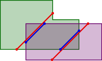
Figure 11: Example interval decomposable multi-parameter persistence module with two interval summands (green and purple), and its barcodes along two lines (here the two couples of red-blue bars). Any matching function induced by, e.g., Wasserstein distances between the barcodes, will match the first red bar with the second red bar and the first blue bar with the second blue bar; however, this matching is not exact.

We show in Section 5.1 that matching functions that are compatible (see Definition 4.11) commute with the matching functions induced by interval decomposable modules. Then, we discuss matching functions induced by the vineyards algorithm in Section 5.2.

5.1 Compatible matching functions

In this section, we show that compatible matching functions commute with the induced matching function $\sigma_{{\mathbb{M}}}$ (when ${\mathbb{M}}$ is interval decomposable) under some specific conditions. In the rest of this section, given a matching function $\sigma$ that commutes with $\sigma_{\mathbb{M}}$, we will also call $\sigma$ exact for the sake of simplicity. Before stating the main result, we first show a technical lemma that relates the locations of endpoints of compatible bars with each other.

Lemma 5.1.

Let $l_{1}$ and $l_{2}$ be two $\delta$-consecutive lines, and let $[b_{1},d_{1}]:={\mathcal{B}}({\left.\kern-1.2ptI\vphantom{\big{|}}\right|_{l_{1}}})$ be the bar of an interval module along $l_{1}$. Let $[b_{2},d_{2}]$ be a bar along $l_{2}$ that is compatible with $[b_{1},d_{1}]$. Then, $d_{2}$ (resp. $b_{2}$) is included in a segment of size $\delta$ in $l_{2}$.

Proof.

Applying Lemma 3.10, one has

$$d_{2}\in C:=\big{[}B_{\delta}(d_{1})\cap l_{2}\big{]}\backslash\big{[}\left\{z\in\mathbb{R}^{n}:z>d_{1}\right\}\cup\left\{z\in\mathbb{R}^{n}:z<d_{1}\right\}\big{]}$$

Since $C$ is a nonempty, totally ordered set, we can define $y:=\min C$. By construction, there exists a dimension $i$ such that $y_{i}\geq(d_{1})_{i}$, and thus $C$ must be included in the segment $[y,y+\delta\cdot\mathbf{1}]$ along $l_{2}$.

The proof applies straightforwardly to $b_{2}$ by symmetry. ∎

Since bars that are matched under an exact matching function are always compatible, one way to construct an exact matching function between two barcodes is therefore to isolate, among all possible matching functions, the ones such that matched bars are compatible. If this family contains a single element, it must be the exact matching we are looking for. This typically happens for interval decomposable multi-parameter persistence module whose summands are sufficiently separared, as we show in the proposition below.

Proposition 5.2.

Let ${\mathbb{M}}=\bigoplus_{I\in\mathcal{I}}I$ be an interval decomposable multi-parameter persistence module. Let $\delta>0$, and $I,I^{\prime}$ be two interval summands in the decomposition of ${\mathbb{M}}$. Assume that the two following properties are satisfied:

1. Let $l\subset\mathbb{R}^{n}$ be a diagonal line such that ${\rm supp}(I)\cap l\neq\varnothing$ and ${\rm supp}(I^{\prime})\cap l\neq\varnothing$. Then, one has either $\left\lVert b_{l}^{I}-b_{l}^{I^{\prime}}\right\rVert_{\infty}>\delta$ or $\left\lVert d_{l}^{I}-d_{l}^{I^{\prime}}\right\rVert_{\infty}>\delta$. In other words, the endpoints of the bar in ${\mathcal{B}}({\left.\kern-1.2ptI\vphantom{\big{|}}\right|_{l}})$ and of the bar in ${\mathcal{B}}({\left.\kern-1.2ptI^{\prime}\vphantom{\big{|}}\right|_{l}})$ are at distance at least $\delta$.

2. The bars of length at most $2\delta$ in $I$ and $I^{\prime}$ are at distance at least $\delta$, i.e., if we let

   $$S^{I}:=\left\{l:l\cap{\rm supp}(I)\neq\varnothing,\left\lVert b_{l}^{I}-d_{l}^{I}\right\rVert_{\infty}\leq 2\delta\right\},$$

   (and similarly for $I^{\prime}$), one has $d_{\infty}(S^{I},S^{I^{\prime}})>\delta/2.$ In other words, a small bar in $I$ cannot be too close to a small bar in $I^{\prime}$.

Then, the matching function $\sigma_{\rm comp}$, induced by matching bars that are compatible together, is well-defined and exact.

See Figure 12 for an illustration of assumptions (1) and (2).

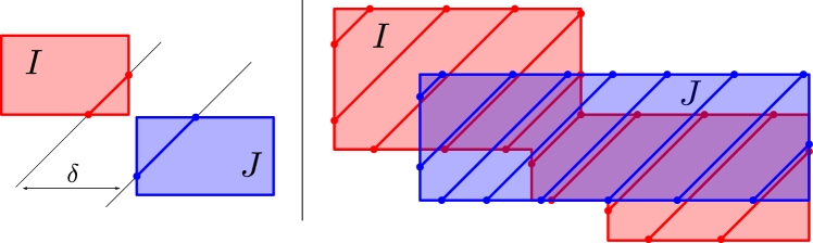
Figure 12: (Left) Example of module whose interval summands do not satisfy assumption (2). (Right) Example of module whose interval summands do satisfy assumptions (1) and (2). Bars corresponding to consecutive lines can only be matched if they are compatible, which, in this figure, means that they have the same color, i.e., that they are associated to the same interval summand.

Proof.

Let $I$ and $I^{\prime}$ be two interval summands in the decomposition of ${\mathbb{M}}$. Let $l_{1}$ and $l_{2}$ be two $\delta$-consecutive lines of $L$, and let $b:={\mathcal{B}}({\left.\kern-1.2ptI\vphantom{\big{|}}\right|_{l_{1}}})$ be the bar corresponding to $I$ along $l_{1}$. We will show that $\sigma_{\rm comp}$ must match $b$ to either $b^{\prime}:={\mathcal{B}}({\left.\kern-1.2ptI\vphantom{\big{|}}\right|_{l_{2}}})$ if ${\rm supp}(I)\cap l_{2}\neq\varnothing$, or the empty set if ${\rm supp}(I)\cap l_{2}=\varnothing$.

• If ${\rm supp}(I)\cap l_{2}=\varnothing$, then by Lemma 3.10, the length of $b$ is at most $\delta$, i.e., $\left\lVert b^{I}_{l_{1}}-d^{I}_{l_{1}}\right\rVert_{\infty}\leq\delta$. It is thus compatible with the empty set. Now, since $d_{\infty}(l_{1},l_{2})=\delta/2$ and since $l_{1}\in S^{I}$, assumption (2) ensures that the bar $b^{\prime\prime}:={\mathcal{B}}({\left.\kern-1.2ptI^{\prime}\vphantom{\big{|}}\right|_{l_{2}}})$ (if it exists) must be of length at least $2\delta$. In particular, it is not compatible with $b$, hence $\sigma_{\rm comp}$ cannot match $b$ to $b^{\prime\prime}$, and must match $b$ to the empty set.

• If ${\rm supp}(I)\cap l_{2}\neq\varnothing$, then the bar $b^{\prime}=[b^{I}_{l_{2}},d^{I}_{l_{2}}]$ in ${\mathcal{B}}({\left.\kern-1.2ptI\vphantom{\big{|}}\right|_{l_{2}}})$ is compatible with $b$, as per Lemma 3.9. According to Lemma 5.1, it follows that the birthpoint and deathpoint of any bar along $l_{2}$ that is compatible to $l_{1}$ must belong to segments $s_{b},s_{d}$ of length $\delta$ that contain $b^{I}_{l_{2}}$ and $d^{I}_{l_{2}}$ respectively. Let $b^{\prime\prime}:=[b^{I^{\prime}}_{l_{2}},d^{I^{\prime}}_{l_{2}}]$ be the bar in ${\mathcal{B}}({\left.\kern-1.2ptI^{\prime}\vphantom{\big{|}}\right|_{l_{2}}})$ (if it exists). According to assumption (1), we either have $\left\lVert b_{l_{2}}^{I}-b_{l_{2}}^{I^{\prime}}\right\rVert_{\infty}>\delta$ or $\left\lVert d_{l_{2}}^{I^{\prime}}-d_{l_{2}}^{I^{\prime}}\right\rVert_{\infty}>\delta$. In particular this means that either $b^{I^{\prime}}_{l_{2}}\not\in s_{b}$ or $d^{I^{\prime}}_{l_{2}}\not\in s_{d}$. Hence $b^{\prime\prime}$ is not compatible with $b$, and $\sigma_{\rm comp}$ must match $b$ to $b^{\prime}$.

In both cases, $\sigma_{\rm comp}$ is well-defined and exact. ∎

5.2 Vineyards matching functions

This section is dedicated to the vineyards algorithm for simplicial complexes. It is quite technical and can be skipped by readers who are most interested in the general exposition. The vineyards algorithm provides a matching function $\sigma_{\rm vine}$ between barcodes, so the purpose of this section is to show that it is exact, i.e., that it commutes with the induced matching function $\sigma_{\mathbb{M}}$, provided that ${\mathbb{M}}$ is interval decomposable. Since vineyards are heavily based on simplicial homology, we first recall the basics of persistent homology from simplicial complexes in Section 5.2.1. Then, we provide an analysis of the vineyards algorithm in Section 5.2.2.

5.2.1 Persistent homology of simplicial complexes

We assume in the following that the reader is familiar with simplicial complexes, boundary operators and homology groups, and we refer the interested reader to [Mun84, Chapter 1] for a thorough treatment of these notions. The first important definition is the one of filtered simplicial chain complexes.

Definition 5.3.

Let $S$ be a simplicial complex, and $f\colon S\to\mathbb{R}$ be a filtration function, i.e., $f$ satisfies $f(\sigma)\leq f(\tau)$ when $\sigma\subseteq\tau$. Then, the filtered simplicial chain complex $(S,f)$ is defined as $(S,f)=((C_{t})_{t\in\mathbb{R}},\iota)$, where

• $C_{t}=\left<\sigma_{0},\dots,\sigma_{i}\right>$ is the vector space over a field $k$ whose basis elements are the simplices that have filtration values smaller than $t$, i.e., $\left\{\sigma_{0},\dots,\sigma_{i}\right\}=\left\{\sigma\in S:f(\sigma)\leq t\right\}$, and

• for any $s\leq t$, the map $\iota=\iota_{s}^{t}\colon C_{s}\hookrightarrow C_{t}$ is the canonical injection.

Note that $f$ can be used to define an order on the simplices of $S=\left\{\sigma_{i}\right\}_{i=0}^{N}$, by using the ordering induced by the filtration values. In other words, we assume in the following that $f(\sigma_{0})\leq f(\sigma_{1})\leq\dots\leq f(\sigma_{N})$. We also slightly abuse notations and define $C_{i}:=\left<\sigma_{0},\dots,\sigma_{i}\right>$ for any $i\in\llbracket 0,N\rrbracket$ and

$$(S,f)=\left(C_{0}\overset{\iota_{0}}{\hookrightarrow}C_{1}\overset{\iota_{1}}{\hookrightarrow}\dots\overset{\iota_{N-1}}{\hookrightarrow}C_{N}=\left<S\right>\right).$$ (11)

Then, applying the homology functor $H_{*}$ on this filtered simplicial chain complex yields the following (single-parameter) persistence module

$$H_{*}(S,f)=0\rightarrow H_{*}(C_{0})\rightarrow H_{*}(C_{1})\rightarrow\dots\rightarrow H_{*}(C_{N}).$$

An important theorem of single-parameter persistent homology states that, up to a change of basis, it is possible to pair some chains together in order to define the so-called one-dimensional persistence barcode associated to the filtered simplicial chain complex.

Theorem 5.4 (Persistence pairing, [dMV11, Theorem 2.6]).

Given a filtered simplicial chain complex $(S,f)=C_{1}\hookrightarrow C_{2}\hookrightarrow\dots\hookrightarrow C_{N}$ and associated persistence module $H_{*}(S,f)$, there exists a partition $\llbracket 1,N\rrbracket=E\sqcup B\sqcup D$, a bijective map ${\rm Low}:D\rightarrow B$, and a new basis $\hat{\sigma}_{1},\dots,\hat{\sigma}_{N}$ of $C$, called reduced basis, such that:

• $C_{i}=\langle\hat{\sigma}_{1},\dots,\hat{\sigma}_{i}\rangle$,

• $\partial\hat{\sigma}_{e}=0$ for any $e\in E$,

• for any $d\in D$, one has $\partial\hat{\sigma}_{{\rm Low}(d)}=0$, and $\partial\hat{\sigma}_{d}$ is equal to $\hat{\sigma}_{{\rm Low}(d)}$ up to simplification, i.e., there exists a set of indices ${\rm bd}(d)$ such that $(i)$ $j<{\rm Low}(d)\leq d$ for any $j\in{\rm bd}(d)$, and $(ii)$ $\partial\hat{\sigma}_{d}=\hat{\sigma}_{{\rm Low}(d)}+\sum_{j\in{\rm bd}(d)}\hat{\sigma}_{j}$.

In particular, the chains $\{\hat{\sigma}_{j}:j\in E\cap\llbracket 1,i\rrbracket\}\cup\{\hat{\sigma}_{j}:j\in B\cap\llbracket 1,i\rrbracket\text{ and }\exists d>i\text{ s.t. }{\rm Low}(d)=j\}$ form a basis of the simplicial homology groups $H_{*}(C_{i})$. Moreover, the chains $\{\hat{\sigma}_{j}:j\in B\sqcup E\}$ are called positive chains while the chains $\{\hat{\sigma}_{j}:j\in D\}$ are called negative chains.

The multiset of bars $\mathcal{B}(f):=\{[f(\hat{\sigma}_{b}),f(\hat{\sigma}_{d})]:b={\rm Low}(d)\}\cup\{[f(\hat{\sigma}_{e}),+\infty):e\in E\}$ is called the persistence barcode of the filtered simplicial chain complex $(S,f)$ and of the single-parameter persistence module $H_{*}(S,f)$.

Note that while the reduced basis $\{\hat{\sigma}_{1},\dots,\hat{\sigma}_{N}\}$ does not need to be unique, the pairing map ${\rm Low}$ is actually independent of that reduced basis (see [EH10, VII.1, Pairing Lemma]).

5.2.2 Vineyards algorithm and matching

The vineyards algorithm is a method that allows to find reduced chain bases for filtered simplicial complexes whose simplex orderings only differ by a single transposition of consecutive simplices, that we denote by $(i\,i+1)$.

Proposition 5.5 ([CSEM06]).

Let $S=\{\sigma_{1},\dots,\sigma_{N}\}$ be a (filtered) simplicial complex (with filtration function $f$), and let $B=\{\hat{\sigma}_{1},\dots,\hat{\sigma}_{N}\}$ be a corresponding reduced chain basis. Let $\tilde{f}:S\rightarrow\mathbb{R}$ be a filtration function that swaps the simplices at positions $i$ and $i+1$, i.e., that induces a new filtered simplicial complex $\tilde{S}=\{\sigma_{1},\dots,\sigma_{i+1},\sigma_{i},\dots,\sigma_{N}\}$. Note that the swapped basis ${\rm sw}_{i}^{S}(B):=\{\hat{\sigma}_{1},\dots,\hat{\sigma}_{i+1},\hat{\sigma}_{i},\dots,\hat{\sigma}_{N}\}$ might not be a reduced basis for $(\tilde{S},\tilde{f})$, since the pairing map ${\rm Low}$ might not be well-defined anymore. Fortunately, there exists a change of basis, called vineyard update, that turns ${\rm sw}_{i}^{S}(B)$ into a reduced basis $\tilde{B}$ of $(\tilde{S},\tilde{f})$ in $O(N)$ time, and that comes with a bijective map $\sigma_{\mathrm{vine}}:B\rightarrow\tilde{B}$, called vineyard matching, that can be used to define a matching $\sigma_{\mathrm{vine}}:{\mathcal{B}}(f)\to{\mathcal{B}}(\tilde{f})$.

Note that the vineyards matching can be straightforwardly extended to filtration functions whose induced ordering differs by a whole permutation from the one of the initial filtration function by simply decomposing the permutation into elementary transpositions (using, e.g., Coxeter decompositions).

Application to multi-parameter persistent homology.

When the simplices of $S$ are (partially) ordered from a function $f:S\rightarrow\mathbb{R}^{n}$, i.e., one has $f(\tau)\leq_{n}f(\sigma)$ for any $\tau\subseteq\sigma$, then the function $f$ is called a multi-parameter filtration function of $S$. In that case, applying the homology functor also leads to simplicial homology groups $\{H_{d}(C_{i})\}_{i\in I}$, where $I\subseteq\llbracket 1,N\rrbracket^{n}$ is the (partial) ordering associated to $f$, and these groups are connected by morphisms as long as their indices are comparable in $\mathbb{R}^{n}$. These groups and maps are called the multi-parameter persistent homology associated to the multi-filtered simplicial chain complex $(S,f)$. Similarly to the single-parameter case, when $k$ is a field, one can define the multi-parameter persistence module ${\mathbb{M}}$ associated to $(S,f)$ as the family of vector spaces indexed over $\mathbb{R}^{n}$ defined with the identifications $M_{s}:=H_{d}(C)$ where $C={\bf{\rm Vect}}\{\sigma\in S:f(\sigma)\leq s\in\mathbb{R}^{n}\}$.

We now show that the vineyards algorithm yields an exact matching function, in the sense that it commutes with the exact matching function induced by the underlying module ${\mathbb{M}}$ when it is interval decomposable.

Proposition 5.6.

Let ${\mathbb{M}}$ be an interval decomposable multi-parameter persistence module computed from a finite multi-filtered simplicial chain complex $(S,f)$ over $\mathbb{R}^{n}$. Then, for a small enough $\delta>0$, $\sigma_{\mathrm{vine}}$ is exact.

Proof.

Let $\delta>0$ be such that, for any two lines $l,l^{\prime}\in L$, there exists a sequence $l=l_{1},\dots,l_{k}=l^{\prime}$ such that the simplex orderings induced by $l_{i}$ and $l_{i+1}$ differ by at most one transposition of two consecutive simplices, for any $i\in\llbracket 1,k-1\rrbracket$.

Let $l,l^{\prime}$ be two diagonal lines in $\mathbb{R}^{n}$, and let $F:={\left.\kern-1.2ptf\vphantom{\big{|}}\right|_{l}}:S\rightarrow\mathbb{R}$ and $F^{\prime}:={\left.\kern-1.2ptf\vphantom{\big{|}}\right|_{l^{\prime}}}\rightarrow\mathbb{R}$. Up to a reordering of the simplices of $S=\left\{\sigma_{1},\dots,\sigma_{N}\right\}$, we assume without loss of generality that $F(\sigma_{1})\leq\dots\leq F(\sigma_{N})$. Let $\mathfrak{S}_{N}^{S}\subseteq\mathfrak{S}_{N}$ be the subset of permutations that satisfies $\tau\in\mathfrak{S}_{N}^{S}\Longrightarrow\left(C^{\tau}_{k}\right)_{k\in\llbracket 1,N\rrbracket}=\left(\left\{\sigma_{\tau(1)},\dots,\sigma_{\tau(k)}\right\}\right)_{k\in\llbracket 1,N\rrbracket}$ is a filtration of $S$. Finally, let $N=(N_{\tau,k})_{(\tau,k)\in\mathfrak{S}_{N}^{S}\times\llbracket 1,N\rrbracket}$, where $N_{\tau,k}=H_{*}(C^{\tau}_{k})$ is the multi-parameter persistence module indexed over $\mathfrak{S}_{N}^{S}\times\llbracket 1,N\rrbracket$, with arrows induced by inclusion. Note that the one-dimensional persistence module $N_{\rm id}:=(N_{{\rm id},k})_{k\in\llbracket 1,N\rrbracket}$ is isomorphic to ${\left.\kern-1.2pt{\mathbb{M}}\vphantom{\big{|}}\right|_{l}}$.

Now, let $\tau$ be the simplex permutation that matches the simplex ordering induced by $F$ to the one induced by $F^{\prime}$. By definition, one has $\tau\in\mathfrak{S}_{N}^{S}$. Let $i$ be the index of the first transposition, i.e., the transposition $(i\,i+1)$ given by the reordering of the simplices from $l=l_{1}$ to $l_{2}$. Then, the matching $\sigma_{\mathrm{vine}}^{i}$ associated to the transposition $(i\,i+1)$ induces a matching between the bars of ${\mathcal{B}}({\left.\kern-1.2pt{\mathbb{M}}\vphantom{\big{|}}\right|_{l}})$ and ${\mathcal{B}}({\left.\kern-1.2pt{\mathbb{M}}\vphantom{\big{|}}\right|_{l_{2}}})$, or equivalently, between the bars of ${\mathcal{B}}(N_{\rm id})$ and ${\mathcal{B}}(N_{(i\,i+1)})$, as well as a morphism between $N_{\rm id}$ and $N_{(i\,i+1)}$. Let us now consider the diamond:

(12)

First, note that all maps in that diamond are either injective of corank 1 or surjective of nullity 1 (since they are all induced by adding a positive or negative chain of the corresponding reduced bases). Moreover, by the Mayer-Vietoris theorem, the following sequence is exact:

$$N_{\text{id},i-1}=N_{(i\,i+1),i-1} =H_{*}(C^{\text{id}}_{i-1})\rightarrow N_{(i\,i+1),i}\oplus N_{\text{id},i}=H_{*}(C^{(i\,i+1)}_{i})\oplus H_{*}(C^{\text{id}}_{i})$$

$$\xrightarrow{(x,y)\mapsto y-x}H_{*}(C^{\text{id}}_{i+1})=N_{\text{id},i+1}=N_{(i\,i+1),i+1}.$$

Such diamonds are called transposition diamonds, and it has been shown in [MO15, Theorem 2.4] that the morphism induced by $\sigma_{\mathrm{vine}}^{i}$ between the lower and upper parts of the diamond matches bars with same representative positive chains together. Hence, bars in ${\mathcal{B}}(N_{\rm id})$ and ${\mathcal{B}}(N_{(i\,i+1)})$, and thus the bars in ${\mathcal{B}}({\left.\kern-1.2pt{\mathbb{M}}\vphantom{\big{|}}\right|_{l_{1}}})$ and ${\mathcal{B}}({\left.\kern-1.2pt{\mathbb{M}}\vphantom{\big{|}}\right|_{l_{2}}})$ are matched under $\sigma_{\mathrm{vine}}$ are associated to the same summand of ${\mathbb{M}}$, and thus are compatible. In particular, when ${\mathbb{M}}$ is decomposable into intervals summands, $\sigma_{\mathrm{vine}}$ is exact. Finally, by repeating this argumentation with the other transpositions induced by the simplices reordering from $l_{i}$ to $l_{i+1}$, for $i=2,\dots,k-1$ one has that the same is true for bars in ${\mathcal{B}}({\left.\kern-1.2pt{\mathbb{M}}\vphantom{\big{|}}\right|_{l}})$ and ${\mathcal{B}}({\left.\kern-1.2pt{\mathbb{M}}\vphantom{\big{|}}\right|_{l^{\prime}}})$.

∎

6 Numerical experiments

In this section, we showcase the performances of MMA. More precisely, we empirically study how the output quality and running time depend on the precision $\delta$ and the number of lines $|L|$. Then, we compare the running times of MMA with those of Rivet [LW15] and the elder-rule staircode (ERS) [CKMW20]. Finally, we investigate how running time is affected by the number of filtrations. All experiments were done on a laptop with AMD Ryzen 4800 CPU and 16GB of RAM. Our code is publicly available at https://github.com/DavidLapous/multipers.

Data sets and filtrations.

In our first two experiments, we focus on two real-world data sets of point clouds. The first ones, called LargeHypoxicRegion, were obtained from immunohistochemistry in [Vip20b]. These are made of a few thousand points, each representing a single cell. The others were obtained from applying time-delay embedding in $\mathbb{R}^{2}$ on time series taken from a few data sets (Wine, Plane, OliveOil, Coffee) from the UCR archive [Che15]. On all of these data sets, we computed bi-filtrations using the standard Vietoris-Rips filtration, and the superlevel sets of a Gaussian kernel density estimation (with bandwidth parameter $0.1d$ where $d$ is the diameter of the dataset), and we applied MMA and its competitors on the corresponding multi-parameter persistence modules in homology dimensions $0$ and $1$ (note that the ERS can only compute dimension $0$).

In our third experiment, we measure the dependence on the number of filtrations using a synthetic data set obtained by sampling $300$ points in the unit square $[0,1]^{2}$, computing their Alpha simplicial complex, and generating $n$ random filtration values on the points.

Finally, it is worth noting that we used multi-parameter edge collapses [AKP22] in order to simplify the multi-parameter persistence modules (without losing information) as much as possible before applying Rivet and MMA. The timing of this simplifications are not taken into account, but they are not the computational bottleneck of our computations. Furthermore, for the LargeHypoxicRegion, we thresholded the Rips edges at $0.02$, leading to simplicial complexes of $\sim 85k$ and $\sim 125k$ simplices respectively, after simplifications.

Convergence of MMA.

We first empirically validate Propositions 3.4 and 4.13 by measuring how far is the output of MMA from the data when the precision parameter $\delta$ decreases and the number of lines in $L$ increases. For this, we used the bottleneck distances between the fibered barcodes (on $100$ random diagonal lines) of the outputs of MMA and the ones of the underlying modules as a proxy for the interleaving distances (since they are practically very difficult to evaluate). We call this the estimated matching distance. Results are displayed in Figure 13. One can see that the convergence is empirically linear with the number of lines $|L|$, which is in line with Propositions 3.4 and 4.13 (since $|L|$ increases linearly as $\delta$ decreases for a fixed $n$). Note that the distance even reaches $0$ on a few cases.

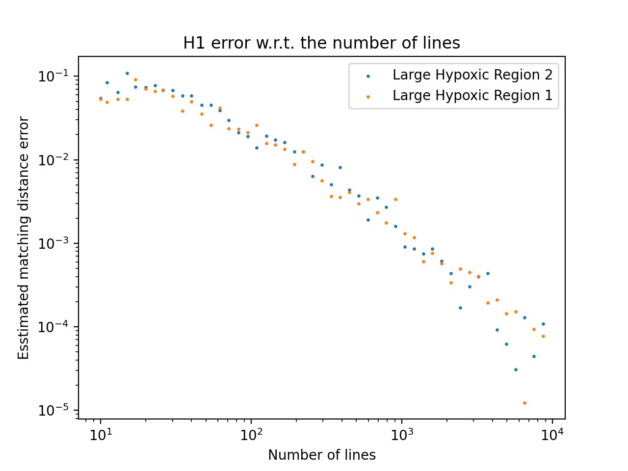
Figure 13: Convergence on UCR data sets (left) and immunohistochemistry data sets (right).

Running times.

We now compare the running times of MMA with those of Rivet and the ERS. Results can be found in Table 1. It is worth noting that on several occasions, Rivet and the ERS could not produce outputs in reasonable time, due (among other things) to large memory consumption. On the other hands, the fact that MMA produces discretely presented intervals allows to encode them in a sparse manner with their corners. Note that computations with Rivet can be also approximated by coarsening the filtration values, and thus the module. In practice, this corresponds to restricting the 2-module to a $\kappa=\kappa_{x}\times\kappa_{y}$ grid, where $\kappa_{x},\kappa_{y}\in\mathbb{N}$ are the resolutions in both axes, see [LW15, Section 8.2]. The parameters $\kappa$ and $|L|$ have (roughly) the same role, and can be related with $\sqrt{\kappa}\simeq|L|$ (for a given, prescribed precision). Overall, we find that the running times of MMA outperforms its competitors, except when $\kappa$ is very small. However, in this case, the corresponding output of Rivet is very crude as the module is restricted on just a few points, whereas MMA produces intervals that are accurate along whole straight lines: we find that for large data sets, MMA is the only method that can produce accurate representations.

	Rivet			ERS	MMA
	$\kappa=10^{2}$	$\kappa=50^{2}$	$\kappa=100^{2}$		$|L|=100$	$|L|=1000$	$|L|=10,000$
Coffee	$0.21\pm 0.01,0.18\pm 0.01$	$9.75\pm 5.92,0.35\pm 0.12$	$--,0.95\pm 0.56$	$0.34\pm 0.04$	$0.0093\pm 0.001$	$0.024\pm 0.001$	$0.16\pm 0.008$
Plane	$0.19\pm 0.005,0.18\pm 0.03$	$4.36\pm 2.24,0.28\pm 0.04$	$33.3\pm 17.5,0.56\pm 0.17$	$0.09\pm 0.03$	$0.004\pm 0.0$	$0.012\pm 0.001$	$0.095\pm 0.004$
Wine	$0.21\pm 0.003,0.19\pm 0.007$	$8.50\pm 2.00,0.22\pm 0.01$	$--,0.28\pm 0.023$	$0.22\pm 0.04$	$0.004\pm 0.0$	$0.016\pm 0.0$	$0.129\pm 0.002$
OliveOil	$0.21\pm 0.004,0.19\pm 0.002$	$5.55\pm 1.20,0.31\pm 0.016$	$--,0.82\pm 0.17$	$1.39\pm 0.03$	$0.026\pm 0.001$	$0.058\pm 0.001$	$0.37\pm 0.006$
Worms	$0.29\pm 0.082,0.23\pm 0.23$	$19.9\pm 14.4,4.60\pm 5.0$	$--,31.36\pm 36.24$	$3.85\pm 0.1$	$0.22\pm 0.11$	$0.34\pm 0.15$	$1.35\pm 0.41$
LargeHypoxicRegion1	$1.73,2.88$	$--,234$	$--,--$	$--$	$26.4$	$26.6$	$59.4$
LargeHypoxicRegion2	$2.39,6.04$	$--,--$	$--,--$	$--$	$57.3$	$54.3$	$102.9$

Table 1: Mean and variances of the running times (s) for Rivet, the ERS and MMA. We provide both degree 0 (left) and 1 (right) homology timings for Rivet, whereas the timings of MMA include both. The double dashes correspond to out of memory errors, i.e., a memory usage that is over $12\mathrm{GB}$.

Interestingly, computing 0-dimensional homology is sometimes slower than 1-dimensional homology for Rivet; as it relies on computing minimal free presentations, we think that this comes from the fact that minimal presentations in homology dimension 0 can be more complex than their counterparts in homology dimension 1, i.e., they have much more generators. We also investigate how running times of MMA depend on the number of lines. Unsurprisingly, one can see from Figure 14 that running time increases with the number of lines. However, the dependency looks empirically sublinear, which could come from the fact that even though there are more lines, these lines are closer to each other, and thus matching them with vineyards requires fewer computation steps. This is also highlighted by the running times of LargeHypoxicRegion2, Table 1 which are smaller when computing it over $1~{}000$ lines than $100$ lines.

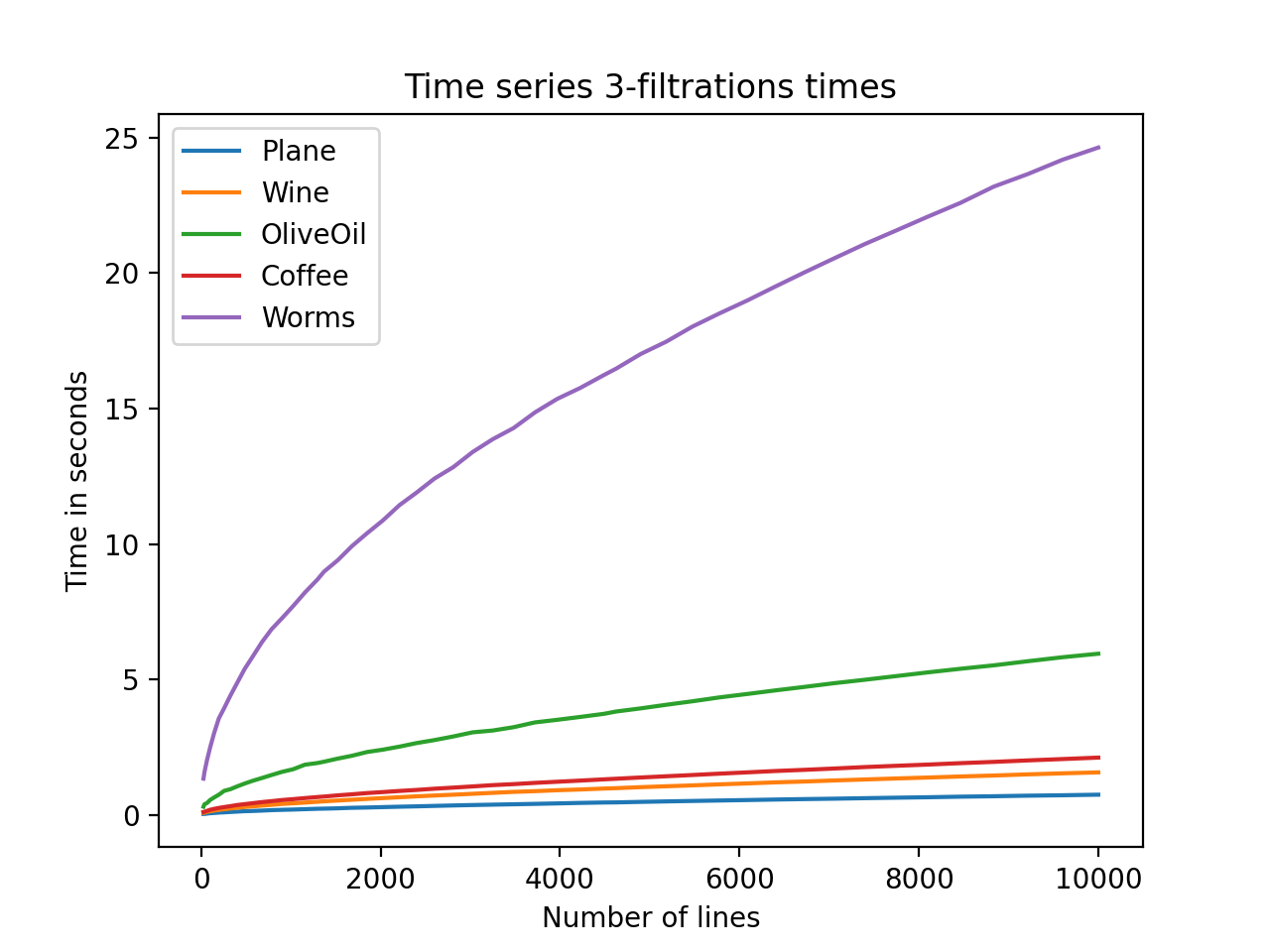
Figure 14: Running time (s) needed to run MMA on the UCR datasets.

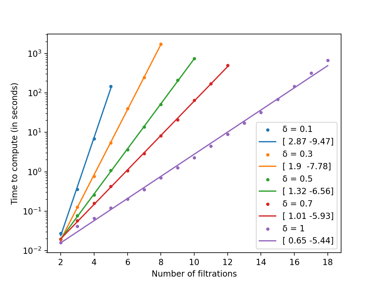
Figure 15: Running time (s) of MMA w.r.t. the number $n$ of filtrations.

Dependence on number of filtrations.

Finally, we investigate how the running times of MMA depend on the number $n$ of filtrations. While most of the approaches in the literature are limited to $n=2$ parameters, one can see from Figure 15 that MMA can produce outputs in a reasonable amount of time for up to $n\simeq 10$ parameter filtrations. As expected from the complexity of MMA in Equation 8, the running times increase exponentially with $n$.

7 Conclusion

In this article, we presented MMA: a new scheme for computing topological invariants (in the form of candidate decompositions) of multi-parameter persistence modules, in a fast and robust way, and whose complexity, running time, and approximation error can be controlled by user-defined parameters. We then showcased the performances of our method on synthetic and real data sets. Our code is publicly available at https://github.com/DavidLapous/multipers.

There are a number of interesting directions for future work.

1. We conjecture that the family of candidate decompositions produced by varying matching functions completely recovers multi-dimensional persistence modules.

2. We proved that our candidate has bounded approximation error when approximating interval decomposable modules. We also proved stability even when the underlying module is not interval decomposable. Is there some kind of optimality result describing the relationship of the candidate decomposition to the underlying module in this case?

3. Recently, stability results have become available for specific multi-parameter persistence modules [BL20]. We expect that these can be used to infer theoretical confidence regions and convergence rates for our candidate decompositions.

References

- [ABE+18] Hideto Asashiba, Mickaël Buchet, Emerson Escolar, Ken Nakashima, and Michio Yoshiwaki. On interval decomposability of 2D persistence modules. In CoRR. arXiv:1812.05261, 2018.
- [AEK+17] Henry Adams, Tegan Emerson, Michael Kirby, Rachel Neville, Chris Peterson, Patrick Shipman, Sofya Chepushtanova, Eric Hanson, Francis Motta, and Lori Ziegelmeier. Persistence images: a stable vector representation of persistent homology. Journal of Machine Learning Research, 18(8):1–35, 2017.
- [AENY19] Hideto Asashiba, Emerson Escolar, Ken Nakashima, and Michio Yoshiwaki. On approximation of 2D persistence modules by interval-decomposables. In CoRR. arXiv:1911.01637, 2019.
- [AKP22] Ángel Javier Alonso, Michael Kerber, and Siddharth Pritam. Filtration-domination in bifiltered graphs. In CoRR. arXiv:2211.05574, 2022.
- [BHO18] Mickaël Buchet, Yasuaki Hiraoka, and Ippei Obayashi. Persistent homology and materials informatics. In Nanoinformatics, pages 75–95. Springer-Verlag, 2018.
- [BL18] Magnus Botnan and Michael Lesnick. Algebraic stability of zigzag persistence modules. Algebraic and Geometric Topology, 18(6):3133–3204, 2018.
- [BL20] Andrew Blumberg and Michael Lesnick. Stability of 2-parameter persistent homology. In CoRR. arXiv:2010.09628, 2020.
- [BL22] Magnus Botnan and Michael Lesnick. An introduction to multiparameter persistence. In CoRR. arXiv:2203.14289, 2022.
- [BLO22] Magnus Botnan, Vadim Lebovici, and Steve Oudot. On rectangle-decomposable 2-parameter persistence modules. Discrete & Computational Geometry, 2022.
- [BLOry] Magnus Botnan, Vadim Lebovici, and Steve Oudot. Local characterizations for decomposability of 2-parameter persistence modules. In CoRR. arXiv:2008.02345, 2020. To appear in Algebras and Representation Theory.
- [BOO21] Magnus Botnan, Steffen Oppermann, and Steve Oudot. Signed barcodes for multi-parameter persistence via rank decompositions and rank-exact resolutions. In CoRR. arXiv:2107.06800, 2021.
- [Bub15] Peter Bubenik. Statistical topological data analysis using persistence landscapes. Journal of Machine Learning Research, 16(3):77–102, 2015.
- [Car09] Gunnar Carlsson. Topology and data. Bulletin of the American Mathematical Society, 46(2):255–308, 2009.
- [CB20] Mathieu Carrière and Andrew Blumberg. Multiparameter persistence image for topological machine learning. In Advances in Neural Information Processing Systems 34 (NeurIPS 2020), pages 22432–22444. Curran Associates, Inc., 2020.
- [CCI+20] Mathieu Carrière, Frédéric Chazal, Yuichi Ike, Théo Lacombe, Martin Royer, and Yuhei Umeda. PersLay: a neural network layer for persistence diagrams and new graph topological signatures. In 23rd International Conference on Artificial Intelligence and Statistics (AISTATS 2020), pages 2786–2796. PMLR, 2020.
- [CCO17] Mathieu Carrière, Marco Cuturi, and Steve Oudot. Sliced Wasserstein kernel for persistence diagrams. In 34th International Conference on Machine Learning (ICML 2017), volume 70, pages 664–673. PMLR, 2017.
- [CdSGO16] Frédéric Chazal, Vin de Silva, Marc Glisse, and Steve Oudot. The structure and stability of persistence modules. SpringerBriefs in Mathematics. Springer-Verlag, 2016.
- [Che15] Chen, Yanping and Keogh, Eamonn and Hu, Bing and Begum, Nurjahan and Bagnall, Anthony and Mueen, Abdullah and Batista, Gustavo. The UCR time series classification archive, 2015.
- [CKMW20] Chen Cai, Woojin Kim, Facundo Mémoli, and Yusu Wang. Elder-rule-staircodes for augmented metric spaces. In 36th International Symposium on Computational Geometry (SoCG 2020), pages 26:1–26:17. Schloss Dagstuhl–Leibniz-Zentrum fuer Informatik, 2020.
- [CO19] Jérémy Cochoy and Steve Oudot. Decomposition of exact pfd persistence bimodules. Discrete & Computational Geometry, pages 1–39, 2019.
- [CSEM06] David Cohen-Steiner, Herbert Edelsbrunner, and Dmitriy Morozov. Vines and vineyards by updating persistence in linear time. In 22nd Annual Symposium on Computational Geometry (SoCG 2006), pages 119–126. Association for Computing Machinery, 2006.
- [DKM22] Tamal Dey, Woojin Kim, and Facundo Mémoli. Computing generalized rank invariant for 2-parameter persistence modules via zigzag persistence and its applications. In 38th International Symposium on Computational Geometry (SoCG 2022), volume 224, pages 34:1–34:17. Schloss Dagstuhl–Leibniz-Zentrum für Informatik, 2022.
- [dMV11] Vin de Silva, Dmitriy Morozov, and Mikael Vejdemo-Johansson. Dualities in persistent (co)homology. Inverse Problems, 27(12):124003, 2011.
- [DW22] Tamal Dey and Yusu Wang. Computational topology for data analysis. Cambridge University Press, 2022.
- [DX21] Tamal Dey and Cheng Xin. Rectangular approximation and stability of 2-parameter persistence modules. In CoRR. arXiv:2108.07429, 2021.
- [DX22] Tamal Dey and Cheng Xin. Generalized persistence algorithm for decomposing multiparameter persistence modules. Journal of Applied and Computational Topology, 2022.
- [EH10] Herbert Edelsbrunner and John Harer. Computational topology: an introduction. American Mathematical Society, 2010.
- [KM18] Woojin Kim and Facundo Mémoli. Generalized persistence diagrams for persistence modules over posets. In CoRR. arXiv:1810.11517, 2018.
- [KR21] Michael Kerber and Alexander Rolle. Fast minimal presentations of bi-graded persistence modules. In Symposium on Algorithm Engineering and Experiments (ALENEX 2021), pages 207–220, 2021.
- [Lan18] Claudia Landi. The rank invariant stability via interleavings. In Research in Computational Topology, pages 1–10. Springer, 2018.
- [Les15] Michael Lesnick. The theory of the interleaving distance on multidimensional persistence modules. Foundations of Computational Mathematics, 15(3):613–650, 2015.
- [LW15] Michael Lesnick and Matthew Wright. Interactive visualization of 2D persistence modules. In CoRR. arXiv:1512.00180, 2015.
- [LW19] Michael Lesnick and Matthew Wright. Computing minimal presentations and bigraded Betti numbers of 2-parameter persistent homology. In CoRR. arXiv:1902.05708, 2019.
- [MO15] Clément Maria and Steve Oudot. Zigzag persistence via reflections and transpositions. In 26th Annual ACM-SIAM Symposium on Discrete Algorithms (SODA 2015), pages 181–199. Society for Industrial and Applied Mathematics, 2015.
- [Mun84] James Munkres. Elements of algebraic topology. CRC Press, 1984.
- [Oud15] Steve Oudot. Persistence theory: from quiver representations to data analysis, volume 209 of Mathematical Surveys and Monographs. American Mathematical Society, 2015.
- [RB19] Raúl Rabadán and Andrew Blumberg. Topological data analysis for genomics and evolution. Cambridge University Press, 2019.
- [RHBK15] Jan Reininghaus, Stefan Huber, Ulrich Bauer, and Roland Kwitt. A stable multi-scale kernel for topological machine learning. In 28th IEEE Conference on Computer Vision and Pattern Recognition (CVPR 2015), pages 4741–4748. IEEE Computer Society, 2015.
- [Vip20a] Oliver Vipond. Local equivalence of metrics for multiparameter persistence modules. In CoRR. arXiv:2004.11926, 2020.
- [Vip20b] Oliver Vipond. Multiparameter persistence landscapes. Journal of Machine Learning Research, 21(61):1–38, 2020.