A statistical comparison of different approximate Hamiltonian-based anharmonic free energy estimators

Abstract

Ensuring a satisfactory statistical convergence of anharmonic thermodynamic properties requires sampling of many atomic configurations, however the methods to obtain those necessarily produce correlated samples, thereby reducing the effective sample size and increasing the uncertainty compared to purely random sampling. In previous works procedures have been implemented to accelerate the computations by first performing simulations using an approximate Hamiltonian which is computationally more efficient than the accurate one and then using various methods to correct for the resulting error. Those rely on recalculating the accurate energies of a random subset of configurations obtained using the approximate Hamiltonian thereby maximizing the effective sample size. This procedure can be particularly suitable for calculating thermodynamic properties using density-functional theory in which case the accurate and approximate Hamiltonians may be represented by parametrically suitably converged and non-converged ones. Whereas it is qualitatively known that there needs to be a sufficient overlap between the phase spaces of the approximate and the accurate Hamiltonians, the quantitative limits of applicability and the relative efficiencies of such methods is not well known. In this paper a statistical analysis is performed first theoretically and then quantitatively by numerical analysis. The sampling distributions of different free energy estimators are obtained and the dependence of their bias and variance with respect to convergence parameters, simulation times and reference potentials is estimated.

I Introduction

Theoretical prediction of anharmonic thermodynamic properties of a material from first principles requires a fast and accurate method to sample the energies of relevant microstates of the atomic system. For instance, in order to obtain good estimates of the phase transition temperatures, the Gibbs free energies typically need to be determined to less than $1\text{\,}\mathrm{m}\mathrm{eV}\mathrm{/}\mathrm{a}\mathrm{t}\mathrm{o}\mathrm{m}$ at high temperatures [1, 2, 3] which is a fraction of a percent of the total free energy. It has been proposed that density functional theory (DFT) [4, 5] based calculations are able to provide such a level of accuracy while taking into account the various contributions to the free energy, such as those from vibrational, electronic and magnetic excitations [6, 7].

An integral part of any DFT calculation is verifying the convergence of the results with respect to various approximations, such as the number of explicitly treated electrons, truncation of the basis set of the wave functions, the number of k-points used to sample the Brillouin zone, smearing of the electronic states, stopping criteria for the optimization of the density and so on [8, 9]. Apart from the lattice dynamics method, which provides an analytic expression [10, 11], calculating the free energy of a crystal is done numerically by sampling atomic configurations using Monte Carlo (MC) or molecular dynamics (MD) simulations [12, 13, 14] and subsequently transforming thermodynamic averages of energy differences to free energy differences. In order to keep the statistical error of the averages low at high temperatures, many simulation steps are needed, which is impractical to accomplish with highly converged DFT. Therefore it has become a standard practice to carry out the simulations using non-converged energies and forces, after which various techniques can be used to adjust the results to correct for the resulting error [15, 16, 3, 17, 7, 18, 19].

This systematic error can be thought of as consisting from the direct error in the computed energies due to the non-convergence and the indirect error due to the sampled structures being different from those that would be obtained from simulations using converged forces and energies. The former can be corrected simply by taking a smaller subset of the sampled configurations and recalculating the energies using parameters that ensure sufficient convergence. This is the idea behind up-sampled thermodynamic integration using Langevin dynamics (UP-TILD) [16, 3] and its two-stage variation (TU-TILD) [17]. In both cases the correction is applied to every step on the thermodynamic integration (TI) [20, 12, 21] path between a harmonic reference and DFT in the case of the former and an empirical potential and DFT when using the latter method.

This approximation is exact in the limit where the energy differences between converged and non-converged calculations do not depend on the atomic configuration, i.e. remain constant throughout the simulation, which implies that the forces are not affected. In general, however, changing DFT parameters can have a considerable effect on the forces. In that case free energy perturbation (FEP) can be used to obtain an estimate of the error either by applying it directly [18], through its truncated cumulant expansion [15, 19] or by reweighting ensemble averages [7]. The latter approach, while strictly speaking not FEP, entails calculating the same exponential averages which can be significantly biased in the limit of a small dataset and can exhibit poor convergence with respect to the size of the dataset [22, 23, 24, 25, 26, 27, 28, 29]. The problem is further exacerbated when FEP is performed unidirectionally [30] as is mostly the case when applying it to adjust the non-converged DFT results.

In this paper first a statistical analysis is performed theoretically, which is helpful to understand some aspects of the different free energy estimators, but is also limited since in general the distributions of energy differences are not known and have to be sampled numerically. In order to accelerate the latter, Spectral Neighbor Analysis Potentials (SNAP) [31] are fitted to DFT-MD data of different levels of convergence. This allows for fast calculations of the sampling distributions of the energy differences between both the reference and the approximate Hamiltonians and between the accurate and the approximate Hamiltonians throughout the whole TI path. From these data the bias and the variance of the different free energy estimators can be computed for different combinations of DFT convergence parameters, expected simulation times and reference potentials.

II Theory and setup

II.1 Free energy estimators

When the potential energy of a system depends on a parameter $\lambda$, the partial derivative of the Helmholtz free energy with respect to $\lambda$ is given by [12]:

$$\left(\frac{\partial F(\lambda)}{\partial\lambda}\right)_{\lambda,NVT}=\left<\frac{\partial U(\lambda)}{\partial\lambda}\right>_{\lambda,NVT}$$ (1)

This can be used to calculate the free energy difference between two states with different potential energies $U_{1{}}$ and $U{{}_{0}}$ by choosing $U(\lambda)$ as

$$U(\lambda)=\lambda U_{1{}}+(1-\lambda)U{{}_{0}}$$ (2)

and integrating both sides of Equation 1 from $\lambda=0$ to $\lambda=1$, giving

$$\left(F_{1}-F_{0}\right)_{NVT}=\int_{0}^{1}\left<U_{1{}}-U{{}_{0}}\right>_{\lambda,NVT}d\lambda$$ (3)

The free energy $F_{1}$ of any system with potential energy $U_{1{}}$ can therefore by estimated by choosing a suitable reference potential $U{{}_{0}}$ for which the free energy $F_{0}$ is known and integrating the potential energy difference between the systems on the path given by Equation 2. Common reference potentials for solids include uncoupled, i.e. Einstein crystal, and coupled harmonic oscillators as in both cases the free energy can be calculated analytically.

In practice the integral can be evaluated by performing several equilibrium MC or MD simulations at different values of $\lambda$ and using, for example, a Gauss-Legendre quadrature or by fitting a function whose integral can be found analytically through the calculated points. Commonly a polynomial of a suitable degree is chosen while the $\lambda$ values can be either equidistant or not [32, 33]. In some cases more sophisticated trigonometric functions have been used in order to get a better fit compared to a polynomial with the same number of parameters [3].

Regardless of the chosen integration method, when DFT-MD is used to estimate the free energy difference, both the errors in the potential energy $U_{1{}}$ and forces ${\vec{f_{1{}}}=-\nabla U_{1{}}}$ due to chosen approximations (DFT convergence) and the uncertainty of the ensemble average at each $\lambda$ (statistical convergence) have to be kept small enough to ensure adequate accuracy of the results.

The natural way to estimate $\mu(\lambda)=\left<U_{1{}}-U{{}_{0}}\right>_{\lambda}$, is to take the arithmetic mean of the samples obtained from MD using potential $U(\lambda)$

$$\hat{\mu}(\lambda)=\frac{1}{N}\displaystyle\sum_{i=1}^{N}\left(U_{1{}}{{}_{i}}-U{{}_{0}}{{}_{i}}\right)$$ (4)

however, due to autocorrelation of the samples, this can be quite inefficient compared to random sampling, since the variance of $\hat{\mu}$ does not decrease in proportion with the sample size $N$, but the effective sample size, $N_{\mathrm{eff}}$ which can be significantly smaller.

If $U_{1{}}$ in Equation 2 is replaced with another potential $U^{\prime}_{1{}}$, such that

$$U^{\prime}(\lambda)=\lambda U^{\prime}_{1{}}+(1-\lambda)U{{}_{0}}$$ (5)

then if

$$\mu^{\prime}(\lambda) =\frac{\left<\left(U_{1{}}-U{{}_{0}}\right)e^{-\beta\lambda\left(U_{1{}}-U^{\prime}_{1{}}\right)}\right>_{{\lambda^{\prime}}}}{\left<e^{-\beta\lambda\left(U_{1{}}-U^{\prime}_{1{}}\right)}\right>_{{\lambda^{\prime}}}}$$ (6a)

$$=\left<U_{1{}}-U{{}_{0}}\right>_{{\lambda^{\prime}}}+\frac{\operatorname{cov}\left(U_{1{}}-U{{}_{0}},e^{-\beta\lambda(U_{1{}}-U^{\prime}_{1{}})}\right)_{{\lambda^{\prime}}}}{\left<e^{-\beta\lambda\left(U_{1{}}-U^{\prime}_{1{}}\right)}\right>_{{\lambda^{\prime}}}}$$ (6b)

it follows that

$$\mu^{\prime}(\lambda)=\mu(\lambda)$$ (7)

The latter can be easily shown, since for any property $A$ that depends on the coordinates and momenta of the atoms,

$$\left<A\right>_{\lambda}=\frac{\left<Ae^{-\beta[U(\lambda)-U^{\prime}(\lambda)]}\right>_{{\lambda^{\prime}}}}{\left<e^{-\beta[U(\lambda)-U^{\prime}(\lambda)]}\right>_{{\lambda^{\prime}}}}$$ (8)

where the subscripts $\lambda$ and ${\lambda^{\prime}}$ denote that the potential energy of the ensemble is $U_{1{}}$ and $U^{\prime}_{1{}}$ respectively.

In order to analyze the advantage of estimating $\mu^{\prime}$ over $\mu$, we will first consider the case when

$$\operatorname{cov}\left(U_{1{}}-U{{}_{0}},e^{-\beta\lambda(U_{1{}}-U^{\prime}_{1{}})}\right)_{\lambda^{\prime}}=0$$ (9)

which, although not explicitly shown in the original work, is the approximation behind the UP-TILD method [16]. The corresponding unbiased estimator of $\mu^{\prime}$ is then

$$\hat{\mu}^{\prime}_{0}(\lambda) =\frac{1}{N}\sum_{i=1}^{N}\left(U_{1{}}{{}_{i}}-U{{}_{0}}{{}_{i}}\right)$$ (10)

$$=\frac{1}{N}\sum_{i=1}^{N}\left(U^{\prime}_{1{i}}-U{{}_{0}}{{}_{i}}\right)+\frac{1}{N}\sum_{i=1}^{N}\left(U_{1{}}{{}_{i}}-U^{\prime}_{1{i}}\right)$$

Note that whereas the subscripts ${\lambda^{\prime}}$ are omitted from this and the following estimators, it is implied that the samples are obtained using the potential $U^{\prime}_{1{}}$.

Using $\hat{\mu}^{\prime}_{0}$ does not provide any possible improvement in efficiency over using $\hat{\mu}$, since it entails first performing the simulation using potential $U^{\prime}(\lambda)$ followed by recalculating the energy of every sample using $U_{1{}}$. However, as pointed out above, for a given sample variance it is equivalent to either take the average $N$ correlated samples or $N_{\mathrm{eff}}$ random samples. The simplest way to do the latter is to calculate the mean of every $k$-th sample such that the autocorrelation function for lag $k$ has decreased to a sufficiently small value. This results in estimators

$$\hat{\mu}^{\prime}_{1}(\lambda) =\frac{k}{N}\sum_{i=1}^{N/k}\left(U_{1{}}{{}_{ki}}-U{{}_{0}}{{}_{ki}}\right)$$ (11)

and

$$\hat{\mu}^{\prime}_{2}(\lambda) =\frac{1}{N}\sum_{i=1}^{N}\left(U^{\prime}_{1{i}}-U{{}_{0}}{{}_{i}}\right)+\frac{k}{N}\sum_{i=1}^{N/k}\left(U_{1{}}{{}_{ki}}-U^{\prime}_{1{{ki}}}\right)$$ (12)

which can be faster to evaluate than $\hat{\mu}$, assuming that it is faster to calculate $U^{\prime}_{1{}}$ compared to $U_{1{}}$. The difference between Equations 11 and 12 is whether all of the original energies are taken into account or only the ones corresponding to the recalculated configurations. This has no direct effect on the computational time, but the variances of the estimators can differ. This will be investigated in more detail in Section III.4.

In order for $\hat{\mu}^{\prime}_{1}$ and $\hat{\mu}^{\prime}_{2}$ to be unbiased, a sufficient condition for $U^{\prime}_{1{}}$ is

$$\operatorname{var}(U_{1{}}-U^{\prime}_{1{}})_{\lambda^{\prime}}=0\quad\forall\lambda\in[0,1]$$ (13)

That is a stronger requirement than that of Equation 9, and when true, means that $k=N$ can be taken in the second term of $\hat{\mu}^{\prime}_{2}$, i.e. only a single recalculation is needed. In practice, the variance does not need to be exactly zero. If Equation 9 is not satisfied, then $\hat{\mu}^{\prime}_{2}$ is a biased and inconsistent estimator of $\mu^{\prime}$, but if the bias is smaller than the required accuracy, the approximation can still be used. Moreover, at $\lambda=0$, Equation 9 is always true, regardless of how large $\operatorname{var}(U_{1{}}-U^{\prime}_{1{}})_{0^{\prime}}$ is, since the potential energy $U^{\prime}(0)$ (in Equation 5) does not depend on $U_{1{}}$. Taking all of the above into account it follows that $U^{\prime}_{1{}}$ should be a close approximation of $U_{1{}}$ up to a constant and a typical choice for that is non-converged DFT.

Without any approximations, $\mu^{\prime}$ can be estimated by using either

$$\hat{\mu}^{\prime}_{3}(\lambda)=\frac{\displaystyle\sum_{i=1}^{N/k}\left(U_{1{}}{{}_{ki}}-U{{}_{0}}{{}_{ki}}\right)e^{-\beta\lambda\left(U_{1{}}{{}_{ki}}-U^{\prime}_{1{ki}}\right)}}{\displaystyle\sum_{i=1}^{N/k}e^{-\beta\lambda\left(U_{1{}}{{}_{ki}}-U^{\prime}_{1{ki}}\right)}}$$ (14)

or

$$\hat{\mu}^{\prime}_{4}(\lambda) =\frac{1}{N}\sum_{i=1}^{N}\left(U^{\prime}_{1{i}}-U{{}_{0}}{{}_{i}}\right)-\frac{k}{N}\sum_{i=1}^{N/k}\left(U^{\prime}_{1{ki}}-U{{}_{0}}{{}_{ki}}\right)$$ (15)

$$+\frac{\displaystyle\sum_{i=1}^{N/k}\left(U_{1{}}{{}_{ki}}-U{{}_{0}}{{}_{ki}}\right)e^{-\beta\lambda\left(U_{1{}}{{}_{ki}}-U^{\prime}_{1{ki}}\right)}}{\displaystyle\sum_{i=1}^{N/k}e^{-\beta\lambda\left(U_{1{}}{{}_{ki}}-U^{\prime}_{1{ki}}\right)}}$$

$$=\hat{\mu}^{\prime}_{2}+\frac{\displaystyle\sum_{i=1}^{N/k}\left(U_{1{}}{{}_{ki}}-U{{}_{0}}{{}_{ki}}\right)e^{-\beta\lambda\left(U_{1{}}{{}_{ki}}-U^{\prime}_{1{ki}}\right)}}{\displaystyle\sum_{i=1}^{N/k}e^{-\beta\lambda\left(U_{1{}}{{}_{ki}}-U^{\prime}_{1{ki}}\right)}}$$

$$-\frac{k}{N}\sum_{i=1}^{N/k}\left(U_{1{}}{{}_{ki}}-U{{}_{0}}{{}_{ki}}\right)$$

the difference being that at the limit of Equation 13 the former approaches $\hat{\mu}^{\prime}_{1}$ and the latter $\hat{\mu}^{\prime}_{2}$ thereby making use of all of the available data.

Both $\hat{\mu}^{\prime}_{3}$ and $\hat{\mu}^{\prime}_{4}$ are biased, but consistent estimators of $\mu^{\prime}$ meaning that as the number of samples $N$ goes to infinity, the bias approaches $0$. However, for small $N$ and large $\operatorname{var}(U_{1{}}-U^{\prime}_{1{}})_{\lambda^{\prime}}$ it is possible that the uncertainty due to the bias and the variance of the exponential ensemble averages [28, 30, 34] is so large that estimating $\mu^{\prime}$ instead of $\mu$ might not provide any improvement or even be less efficient. An exception to that is when ${(U_{1{}}-U{{}_{0}})_{\lambda^{\prime}}}$ and ${(U_{1{}}-U^{\prime}_{1{}})_{\lambda^{\prime}}}$ follow a bivariate normal distribution. In that case Equation 6 simplifies to

$$\mu^{\prime}_{\mathcal{N}}(\lambda)=\left<U_{1{}}-U{{}_{0}}\right>_{{\lambda^{\prime}}}-\lambda\beta\operatorname{cov}\left(U_{1{}}-U{{}_{0}},U_{1{}}-U^{\prime}_{1{}}\right)_{\lambda^{\prime}}$$ (16)

which can be estimated without bias since the sample covariance is an unbiased estimator of the ensemble covariance.

For any estimator $\hat{\mu}^{\prime}$ disrobed above the free energy difference $F_{1}-F_{0}$ is estimated as

$$\Delta\hat{F}(N,k)=\int_{0}^{1}\hat{\mu}^{\prime}(\lambda;N,k)d\lambda$$ (17)

It is noteworthy that even if $\hat{\mu}^{\prime}$ is biased at almost every $\lambda$, it is possible that $\Delta\hat{F}$ is unbiased, if the bias integrates to $0$, for example when using $\hat{\mu}^{\prime}_{2}$ and

$$\int_{0}^{1}\operatorname{cov}\left(U_{1{}}-U{{}_{0}},e^{-\beta\lambda(U_{1{}}-U^{\prime}_{1{}})}\right)_{\lambda^{\prime}}d\lambda=0$$ (18)

Figure 1: A scheme for obtaining the sampling distribution and the statistics of a free energy estimator. Refer to the text for a detailed explanation.

Based on the computational results in this work, it can be hypothesized that for a given $U_{1{}}$ and $U^{\prime}_{1{}}$ it is in principle possible to find $U{{}_{0}}$ such that Equation 18 is true, however doing that might be impractical. Nevertheless the choice of $U{{}_{0}}$ is important, since for random variables $X$ and $Y$

$$|\operatorname{cov}(X,Y)|\leq\sqrt{\operatorname{var}(X)\operatorname{var}(Y)}$$ (19)

i.e. minimizing $\operatorname{var}(U_{1{}}-U{{}_{0}})_{\lambda^{\prime}}$ will reduce the bias, especially when $\lambda$ is close to $1$. This argument also applies to other estimators of $\mu^{\prime}$. In this paper the significance of that is studied by comparing several different reference potentials.

The integral of the first term of both $\hat{\mu}^{\prime}_{2}$ and $\hat{\mu}^{\prime}_{4}$ estimates

$$\int_{0}^{1}\left<U^{\prime}_{1{}}-U{{}_{0}}\right>_{\lambda^{\prime}}d\lambda=F_{1}^{\prime}-F_{0}$$ (20)

Therefore the integral of the other terms estimates

$$F_{1}-F_{0}-(F_{1}^{\prime}-F_{0})=F_{1}-F_{1}^{\prime}$$ (21)

i.e. the free energy difference between states with potentials $U_{1{}}$ and $U^{\prime}_{1{}}$. Varying $\lambda$ from 0 to 1, however switches the potential from $U{{}_{0}}$ to $U^{\prime}_{1{}}$. It can be argued that except when Equation 18 is true, as described above, there is no obvious reason to expect that estimating the free energy difference $F_{1}-F_{1}^{\prime}$ via a path that does not directly connect the corresponding states is more efficient than that which does. Typically $U{{}_{0}}$ is a significantly worse approximation of $U_{1{}}$ than $U^{\prime}_{1{}}$, in which case the samples of $U_{1{}}-U^{\prime}_{1{}}$ near $\lambda=0$ provide much less information about $F_{1}-F_{1}^{\prime}$ than those near $\lambda=1$ so it might be advantageous to just gather more samples at that endpoint of the path.

Moreover, since successful application of either $\hat{\mu}^{\prime}_{2}$ or $\hat{\mu}^{\prime}_{4}$ requires $\operatorname{var}(U_{1{}}-U^{\prime}_{1{}})_{\lambda^{\prime}}$ to be as small as possible anyway, it could be more reasonable to calculate $F_{1}-F_{1}^{\prime}$ directly using FEP from

$$\Delta F_{11^{\prime}}=F_{1}-F^{\prime}_{1}=-\beta^{-1}\ln\left<e^{-\beta(U_{1}-U^{\prime}_{1})}\right>_{\lambda^{\prime}=1}$$ (22)

When $(U_{1{}}-U^{\prime}_{1{}})_{{\lambda^{\prime}}=1}$ has a Gaussian distribution, a second order cumulant expansion of FEP (FEP-$\mathcal{N}$)can be used as

$$\Delta F_{11^{\prime}}=F_{1}-F^{\prime}_{1}=\left<U_{1{}}-U^{\prime}_{1{}}\right>_{\lambda^{\prime}=1}-\frac{\beta}{2}\operatorname{var}(U_{1{}}-U^{\prime}_{1{}})_{\lambda^{\prime}=1}$$ (23)

which has the advantage of converging much faster than the full FEP [34] and being able to estimate it without bias. When estimating $F_{1}-F^{\prime}_{1}$, then similarly to $\hat{\mu}^{\prime}$ it is advantageous to take the averages over uncorrelated samples. If every k-th sample is used, the corresponding estimators are

$$\Delta\hat{F}_{11^{\prime}}=-\beta^{-1}\ln\frac{k}{N}\sum_{i=1}^{N/k}e^{-\beta\Delta U_{ki}}$$ (24)

and

$$\Delta\hat{F}_{11^{\prime},\mathcal{N}} =\frac{k}{N}\sum_{i=1}^{N/k}\Delta U_{ki}$$ (25)

$$-\frac{\beta}{2}\frac{1}{N/k-1}\sum_{i=1}^{N/k}\left(\Delta U_{ki}-\overline{\Delta U_{k}}\right)^{2}$$

where $\Delta U_{ki}=U_{1{}}{{}_{ki}}-U^{\prime}_{1{{ki}}}$ and $\overline{\Delta U_{k}}=(k/N)\sum_{i=1}^{N/k}\Delta U_{ki}$, both sampled at $\lambda=1$ with $U^{\prime}_{1{}}$.

II.2 Uncertainties of the estimators

For the given potentials $U{{}_{0}}$, $U_{1{}}$ and $U^{\prime}_{1{}}$, i.e. the reference, accurate and the approximate one respectively, all the described estimators of $\Delta F$ are expected to differ in accuracy and precision. Whereas it might be possible to quantify those by theoretical means, starting from the $\lambda$-dependent multivariate distributions of the potential energies together with a model of time correlations, in practice it is easier to obtain the sampling distributions of the different $\Delta\hat{F}$ and their dependence on $N$ and $k$ using simulations. This also avoids making any assumptions about the underlying distributions or whether other approximations such as the central limit theorem can be applied.

In order to get a sufficiently converged sampling distribution, enough values of $\Delta\hat{F}$ have to be calculated. If the number of those is $m$, then that also requires $m$ values of $\hat{\mu}^{\prime}$ at $n_{\lambda}$ values of $\lambda$, which results in a total number of $mn_{\lambda}$ simulations. However, because the values of $\hat{\mu}^{\prime}$ at any $\lambda$ are uncorrelated with the values at any other $\lambda$, the aforementioned calculations can in fact provide $m^{n_{\lambda}}$ estimates of $\Delta\hat{F}$. If there are more than $m$ values of $\hat{\mu}^{\prime}$ to pick $m$ out of, the number of estimates increases even more and even for modest values of $m$ and $n_{\lambda}$ it becomes vast. A small subset of those, in this work obtained by random sampling, can be used to estimate the sampling distribution of $\Delta\hat{F}$.

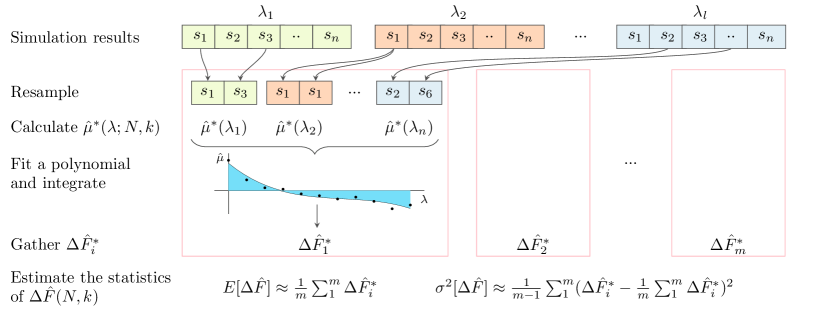
The simplified overview of the method used here is explained in Figure 1. First, at each $\lambda$ a series of MD simulations, differing only by the initial conditions, are run in order to precompute sufficiently representative samples of $U{{}_{0}}$, $U_{1{}}$ and $U^{\prime}_{1{}}$. Alternatively a single long simulation could be performed, however it has been shown that the former helps with faster spanning of the phase space and improving parallelization [35].

Table 1: DFT parameters

Parameter	DFT-0	DFT-1	DFT-2	DFT-3	DFT-4
Cutoff energy ($\mathrm{eV}$)	400.0	223.1	167.3	223.1	167.3
K-points ($\Gamma$-centered)	$\mathrm{4\times 4\times 4}$	$\mathrm{2\times 2\times 2}$	$\mathrm{2\times 2\times 2}$	$\mathrm{1\times 1\times 1}$	$\mathrm{1\times 1\times 1}$
FFT grid	$\mathrm{64\times 64\times 64}$	$\mathrm{36\times 36\times 36}$	$\mathrm{32\times 32\times 32}$	$\mathrm{36\times 36\times 36}$	$\mathrm{32\times 32\times 32}$
Fine FFT grid	$\mathrm{128\times 128\times 128}$	$\mathrm{72\times 72\times 72}$	$\mathrm{48\times 48\times 48}$	$\mathrm{72\times 72\times 72}$	$\mathrm{48\times 48\times 48}$
Projection space	reciprocal	real	real	real	real
Stopping tolerance	$1.0^{-6}$	$1.0^{-6}$	$1.0^{-6}$	$1.0^{-6}$	$1.0^{-4}$
XC-functional	Perdew-Burke-Ernzerhof generalized gradient approximation
Electrons per atom	6
Occupancy smearing	Fermi-Dirac, $\sigma=$0.318\text{\,}\mathrm{eV}$$
Relative speed	1	16	28	50	95

In the next step $m$ estimates of $\Delta F$ are obtained. This is achieved by first choosing the number of timesteps $N$ and the constant $k$. Then the estimators $\hat{\mu}(\lambda;N,k)$ are applied to the data which are resampled with replacement from the set of precomputed short simulations such that the total number of timesteps is $N$. For example, if the number of timesteps in a single simulation was $5000$ and $N=20000$, the results of 4 randomly chosen simulations are combined together. Since the simulations are independent, the correlations in the time series which reduce the effective sample size are trivially preserved. In order to simplify the analysis, $N$ is here taken to be constant with respect to $\lambda$. Next a polynomial is fitted through the obtained $\hat{\mu}(\lambda)$ data points. The degree of the polynomial is chosen such that the leave-one-out cross-validation score is minimized in order to avoid overfitting. The integral of the polynomial from $\lambda=0$ to $\lambda=1$ is then stored.

In the third step the expected value and variance of $\Delta\hat{F}$ can be obtained from the estimates of $\Delta F$ computed in the previous step. For a good estimate of the bias, the reference $\Delta F$ is computed from the integral of Equation 4 with all the available data.

As mentioned, the scheme in Figure 1 is a slight simplification as in practice the different means in $\hat{\mu}^{*}$ were calculated, fitted to a different order polynomials and integrated separately. This allows for analyzing the contributions of the different parts to the uncertainty of $\hat{F}$. In addition, since $k$ can be relatively large (at the limit equal to $N$), in order to better utilize the available data and converge the sampling distributions of $\hat{F}$ faster, each of the simulations was resampled with random starting offset between the first and the k-th timestep.

This approach of obtaining the sampling distribution closely resembles the bootstrap method [36]. The main difference here is that the resampled sample sizes are considerably smaller than the original dataset which results in more accurate sampling distributions. In other words, when enough data have been precalculated, the error made by sampling from those instead of the canonical distribution becomes insignificant. This can be checked, for example, by dividing the precalculated data into multiple chunks, calculating the sampling distributions from each of those separately, and verifying that the results do not vary appreciably.

II.3 Potentials

Several useful conclusions about the statistics of the different $\hat{F}$ could likely be drawn by performing numerical simulations using any reasonable set of $U{{}_{0}}$, $U^{\prime}_{1{}}$ and $U_{1{}}$ even without any DFT calculations. For example, a simple analytical potential could be taken as $U_{1{}}$ and small perturbations made to its parametrization in order to obtain $U^{\prime}_{1{}}$. Although being simple to implement and very fast, this would not provide much quantitative information about realistic problems which could solved using DFT. On the other hand, even with the resampling method described above, resources are limited to calculate everything using DFT-MD. A compromise can be made by performing the analysis with less computationally expensive potentials fitted to DFT. In this work, the choice is quadratic SNAP [31] due to its good and tunable accuracy and ease of fitting, while being orders of magnitude faster than DFT.

A 54-atom supercell of BCC tungsten with lattice parameter of $3.242\text{\,}\mathrm{\SIUnitSymbolAngstrom}$ was chosen as the system to be investigated. The training data were calculated using vasp [37, 38, 39, 40] with projector-augmented wave method [41]. The convergence parameters used for the reference (DFT-0) and the successively worsely converged (DFT-1 to DFT-4) electronic structure calculations are given in Table 1. The canonical ensemble was sampled at $3687\text{\,}\mathrm{K}$ using Langevin dynamics with $10\text{\,}\mathrm{p}\mathrm{s}^{-1}$ friction coefficient and $5\text{\,}\mathrm{fs}$ timestep.

As shown in Table 1, the speedup achieved by using non-converged instead of converged DFT-MD was between one and two orders of magnitude, with the fastest and slowest calculation taking 152 and 14457 core-seconds per timestep respectively. Recalculating the energies using DFT-0 for structures sampled by non-converged DFT-MD was however two times slower, 28230 core-seconds per timestep. This is due to the high correlation between subsequent samples in MD allowing for prediction of the wavefunctions which results in faster convergence of the electronic structure. Given that the recalculation is typically done for uncorrelated samples, this sort of prediction is not applicable.

The fitting was done using fitsnap [42]. The training data consisted of energies and forces of 5374 and 7000 configurations for DFT-0 and the non-converged DFT respectively. The maximum order of the bispectrum components was set to $J_{\textrm{max}}=4$, cutoff distance to $R_{\textrm{max}}=$4.8\text{\,}\mathrm{\SIUnitSymbolAngstrom}$$ and the maximum latitude for remapping neighbor positions to $\theta_{0}^{\textrm{max}}=0.99363\pi$. In order to handle short atomic distances, Ziegler-Biersack-Littmark potential was added with smooth transition to zero between $R_{\textrm{zbl,i}}=$4.0\text{\,}\mathrm{\SIUnitSymbolAngstrom}$$ and $R_{\textrm{zbl,o}}=$4.8\text{\,}\mathrm{\SIUnitSymbolAngstrom}$$.

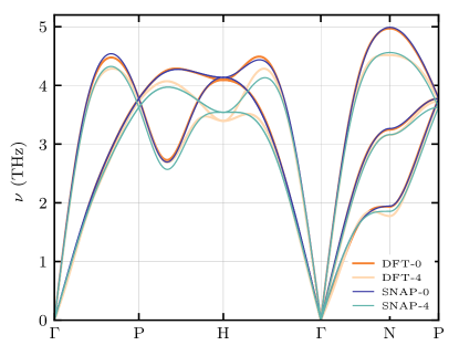
Among all of the fitted potentials, the lowest root mean square errors of energy per atom and force components were $2.6\text{\,}\mathrm{meV}$ and $0.13\text{\,}\mathrm{eV}\mathrm{/}\mathrm{\SIUnitSymbolAngstrom}$ for SNAP-0 (fitted to DFT-0) and the largest errors were $4.4\text{\,}\mathrm{meV}$ and $0.22\text{\,}\mathrm{eV}\mathrm{/}\mathrm{\SIUnitSymbolAngstrom}$ for SNAP-4 (fitted to DFT-4). This is also illustrated on Figure 2, which depicts the phonon dispersions of the harmonic temperature-dependent effective potentials (TDEP) [43] fitted to the high temperature MD data for DFT and the corresponding SNAP. There is very little difference between SNAP-0 and DFT-0 and whereas the error is slightly larger between SNAP-4 and DFT-4, the former is able to adequately reproduce the overall decrease in the effective frequencies caused by non-converged DFT.

The average computational cost of SNAP during the molecular dynamics simulations was 0.02 core-seconds per timestep, i.e. 4 to 6 orders of magnitude faster than DFT.

Figure 2: High temperature phonon dispersions of DFT and SNAP. The force constant matrices were fitted to forces and displacements obtained from $3687\text{\,}\mathrm{K}$ molecular dynamics simulations.

Figure 3: Comparison of the $0\text{\,}\mathrm{K}$ phonon dispersions of DFT and SNAP.

II.4 Reference potentials and switching calculations

Almost any potential can be used as $U{{}_{0}}$, given its free energy is known or can be calculated by another simulation. A simple and easily obtainable choice is the harmonic approximation (HA) of the target potential whose free energy has to be estimated. However, because here $U^{\prime}_{1{}}$ is used for sampling and $U_{1{}}$ for recalculations, it is not clear whether the HA of one should be preferred over that of the other. One one hand, the closer the reference potential is to the target, the more efficient the $\lambda$-switching calculation, which suggests using the HA of $U^{\prime}_{1{}}$. On the other hand, the configurations sampled with a potential more similar to that which is used for recalculating the energies, might make the computationally more expensive recalculations more efficient, suggesting the use of the HA of $U_{1{}}$.

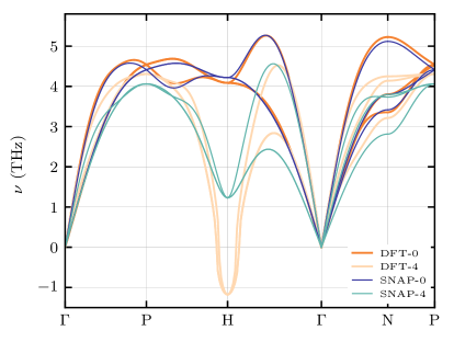
An exception to when the HA could be used as a reference is when some of the phonons have imaginary frequencies since then the free energy is not real-valued. This happens to be the case with DFT-4 near the H-point as shown on Figure 3. Despite that the SNAP training data consisted of only high temperature MD forces and energies, the $0\text{\,}\mathrm{K}$ phonon dispersions were still adequately reproduced while not containing any imaginary frequencies. Therefore the HAs of the fitted potentials were used instead of the DFT ones.

With increasing anharmonicity, the $0\text{\,}\mathrm{K}$ HA is expected by definition to become a successively worse reference potential in terms of efficiency. An improved reference can be obtained by fitting another potential that can take the anharmonicity either implicitly or explicitly into account. In this work two types of such potentials were used. The first ones were the effective harmonic ones described above. The advantage of those is that the reference free energy is known analytically and no extra simulations are needed. The second ones were simpler linear SNAPs (from here on referred to as POT in order to avoid confusing it with the SNAPs approximating DFT) [44] with reduced maximum order of bispectrum components ($J_{\textrm{max}}=3$) compared to the DFT-based potentials and the other parameters unmodified. Using those the reference free energy needs to be calculated separately and whereas this requires setting up simulations and performing additional analysis, the improvement in efficiency can be significant [17]. As with the HA reference, since it is not immediately obvious whether the fitted potentials should be based on $U^{\prime}_{1{}}$ or $U_{1{}}$, both were compared in this work. Since using the latter to directly sample the configurations can be computationally expensive, it might instead be necessary to use the recalculated energies and forces for fitting, the effect of which is also investigated.

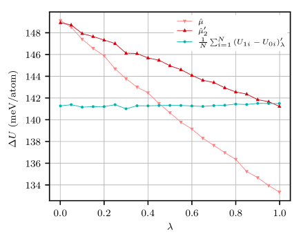
All the simulations were performed using lammps [45]. In order to shorten the equibliration time, the initial positions and velocities were randomly sampled from distributions determined by the HA of the target potential [35]. The canonical ensemble was sampled at $3687\text{\,}\mathrm{K}$ by a Generalized Langevin Equation thermostat [46, 47] with a timestep of $1\text{\,}\mathrm{f}\mathrm{s}$. The drift matrix of the thermostat was generated for optimal sampling in frequency range between 0.07 and $7\text{\,}\mathrm{T}\mathrm{H}\mathrm{z}$. Each simulation consisted of $12\text{\,}\mathrm{p}\mathrm{s}$ out of which the first $2\text{\,}\mathrm{p}\mathrm{s}$ was equibliration. Every 10th configuration was stored and later recalculated using, resulting in 1000 $U_{1{}}$, $U^{\prime}_{1{}}$ and $U{{}_{0}}$ values per simulation. The total number of simulations at each $\lambda$ (21 equidistant values between 0 and 1) was 200 for the HA and TDEP references, and 60 for the POT ones. An example of the results is shown in Figure 4.

Due to the combination of the chosen geometry of the simulation box, lattice type and high temperature, occasionally the whole crystal rotated relative to the box to another symmetry-equivalent configuration. Whereas this did not pose a problem to the SNAP potentials, due to the fixed reference positions the displacements for evaluating the harmonic energies and forces became erroneous. In this case the results of the simulation were discarded and another one with different initial conditions was performed. Since the number of those was relatively low due to the short simulation times, about 1% at $\lambda=1$ and none at $\lambda=0$ since the harmonic potential constrains that type of rotation, the effect on the results is expected to be minimal. Another solution would be to use a supercell for which such rotations are not possible, such as $4\times 4\times 4$ instead of $3\times 3\times 3$.

Figure 4: The $\lambda$-dependent expected values of $\hat{\mu}$, $\hat{\mu}^{\prime}_{2}$ and $\hat{\mu}^{\prime}_{4}$. HA was used as $U{{}_{0}}$ and SNAP-4 as $U^{\prime}_{1{}}$. The expected value was estimated by averaging over all of the available data with $k=1$.

III Results

III.1 The effect of reference systems

Figure 5: Dependence of the variabilities and biases of different $\Delta F$ estimators on various reference potentials and the fraction of recalculated structures for a simulation time of $10\text{\,}\mathrm{ps}$ and SNAP-4 as the potential $U^{\prime}_{1{}}$. The variability is expressed as half of the range that contains 95% of the sampled free energies. Since the sampling distributions were approximately normal, this is close to $1.96\sigma(\Delta\hat{F})$. The bias is defined as $E[\Delta\hat{F}]-\Delta F$, where $\Delta F$ was estimated using all of the available data and the estimator $\hat{\mu}$. The dashed and solid lines denote that SNAP-4 and SNAP-0 were used respectively to obtain the reference potential. The dashed and dotted lines indicate that the fitting was done using forces and energies recalculated using SNAP-0 of the configurations sampled by SNAP-4.

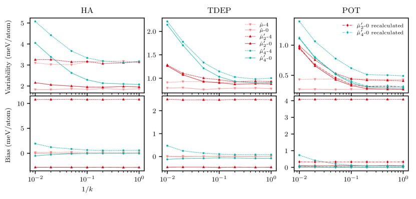
It was qualitatively explained in Section II.1 how the choice of the reference system could affect the accuracy of the results, but without knowing the specific potentials involved, it was not possible to predict how much difference does it make in practice. The results of using either HA, TDEP or POT as $U{{}_{0}}$ and SNAP-4 as $U^{\prime}_{1{}}$ are given in Figure 5.

As expected, in terms of variability, POT is the best reference, followed by TDEP and HA. Using the former makes it possible to determine both $\Delta F(\hat{\mu}^{\prime}_{2})$ and $\Delta F(\hat{\mu}^{\prime}_{4})$ to a precision of less than 1 meV/atom with a relatively short simulation time of $10\text{\,}\mathrm{ps}$ and only about 10 to 20 recalculated energies at each $\lambda$. With the other two references the variance of $U^{\prime}_{1{}}-U{{}_{0}}$ increases the baseline of the uncertainty significantly so either more recalculations, longer simulations, or both are needed to achieve similar precision. In each case the variance of $\Delta\hat{F}(\hat{\mu}^{\prime}_{2})$ is smaller than that of $\Delta\hat{F}(\hat{\mu}^{\prime}_{4})$ meaning that for a given target precision, the former is a more efficient estimator, however the difference becomes smaller with a better reference system.

The situation becomes different and more complex when the bias is also taken into account. Firstly, in every case the bias of $\Delta\hat{F}(\hat{\mu}^{\prime}_{4})$ is smaller than that of $\Delta\hat{F}(\hat{\mu}^{\prime}_{2})$ and at least for the small system considered also significantly smaller than the variability. Interestingly, the bias of $\Delta\hat{F}(\hat{\mu}^{\prime}_{2})$ can be excessive even when using a good reference system. In addition, it is not necessarily easy to quantify without directly comparing $\hat{\mu}^{\prime}_{2}$ and $\hat{\mu}$. For example, it has been proposed that one of the measures for the applicability of the UP-TILD method is that the correction term $\frac{k}{N}\sum_{i=1}^{N/k}\left(U_{1{}}{{}_{ki}}-U^{\prime}_{1{{ki}}}\right)$ would be nearly independent of $\lambda$ [16]. As shown in Figure 6, this is not always the case. With POT fitted to SNAP-4 as $U{{}_{0}}$ this term varies by much less than 1 meV/atom, whereas the bias of $\hat{\mu}^{\prime}_{2}$ grows linearly with $\lambda$ and is over 4 meV/atom for $\Delta\hat{F}$. Conversely, with POT fitted to SNAP-0 as $U{{}_{0}}$, the correction term changes by 7.9 meV/atom between $\lambda=0$ and $\lambda=1$, while the bias is negligible. In short, the estimator of the bias based on the proposal above could itself be biased.

Figure 6: The switching curves from POT fitted to SNAP-4 at $\lambda=0$ to SNAP-4 at $\lambda=1$. Each point is averaged over a $60\text{\,}\mathrm{ps}$ simulation. In $\hat{\mu}^{\prime}_{2}$ and the correction term all of the energies were recalculated, i.e. $k=1$ in Equation 12.

Figure 7: Comparison of the performance of using $\hat{\mu}^{\prime}_{2}$ and $\hat{\mu}^{\prime}_{4}$ for estimating $\Delta F$. The points in increasing order of the CPU time on each line correspond to 10, 20, 50 and 100 ps simulation times at each of the 11 equidistant $\lambda$ values. The dotted, dashed-dotted, dashed and solid lines denote 10, 20, 50 and 100 recalculations at each $\lambda$ respectively. Horizontal solid and dashed are at 1/1.96 and 1/2.58 meV/atom, i.e. the values at which in the absence of bias 95% and 99% of the results would be within 1 meV of the true $\Delta F$. For reference, the corresponding CPU times when using SNAP-0 and $\hat{\mu}$ would be $11\cdot 10^{3}$ and $20\cdot 10^{3}$ core-hours. $\sigma$ denotes the standard deviation and $\mathrm{RMSE}^{2}=E[(\Delta\hat{F}-\Delta F)^{2}]$. The CPU time for each $U^{\prime}_{1{}}$ is the estimated computational time if the corresponding approximation of DFT was used.

Given that the bias of $\Delta\hat{F}(\hat{\mu}^{\prime}_{4})$ is typically significantly smaller than that of $\Delta\hat{F}(\hat{\mu}^{\prime}_{2})$, then the latter can also be approximated as

$$E[\Delta\hat{F}(\hat{\mu}^{\prime}_{2})]-\Delta F \approx E[\Delta\hat{F}(\hat{\mu}^{\prime}_{2})]-E[\Delta\hat{F}(\hat{\mu}^{\prime}_{4})]$$ (26)

$$=\int_{0}^{1}E\left[\hat{\mu}^{\prime}_{2}-\hat{\mu}^{\prime}_{4}\right]d\lambda$$

Since in practice the expectation values in the equation above will be replaced by a single sample, the estimate of the bias can have large uncertainty for large values of $k$. This can make it less useful in the cases where $\operatorname{var}[\Delta\hat{F}(\hat{\mu}^{\prime}_{4})]$ is significantly larger than $\operatorname{var}[\Delta\hat{F}(\hat{\mu}^{\prime}_{2})]$, however, it is asymptotically correct.

As evident, there can be a significant difference in the results whether the reference potential is fitted to $U_{1{}}$ or $U^{\prime}_{1{}}$. In every case the former is a better choice with the largest change observed in the bias of $\Delta\hat{F}(\hat{\mu}^{\prime}_{2})$. There is also a great improvement in both the variance and the bias when the reference potential is fitted indirectly to $U_{1{}}$ by first sampling the configurations using $U^{\prime}_{1{}}$ and then recalculating the energies and forces of those using $U_{1{}}$ to be used in the fitting database. Whereas those configurations are not necessarily the same as those from direct sampling, it can be expected that the fitted potential is at least somewhat transferable, therefore providing an improvement.

Figure 8: Estimates of the biases of $\hat{\mu}^{\prime}_{2}(\lambda)$ for different $U^{\prime}_{1{}}$. The integrals of the curves are the biases of $\Delta\hat{F}(\hat{\mu}^{\prime}_{2})$.

III.2 Choice of the approximate Hamiltonian

Figure 9: The bias and standard deviation of $F_{1}-F_{1}^{\prime}$ estimated by free energy perturbation from a $50\text{\,}\mathrm{ps}$ simulation. The solid and dashed line denote the exact (Equation 24) or the approximate (Equation 25) equation was used. Note that the scale in the bias plot is linear between $-10^{-2}$ and $10^{2}$ meV/atom and logarithmic otherwise.

Choosing which DFT parameters to modify in order to speed up the calculations is not obvious. For the sake of argument, suppose that using Equation 12 does not result in excessive bias so it can be used to obtain good estimates of $\Delta F$ and in addition the covariance between the first and the second term is zero, in which case the total variance is the sum of the variances of the two terms. If $U^{\prime}_{1{}}$ is a close approximation of $U_{1{}}$, then by definition ${\operatorname{var}(U^{\prime}_{1{}}-U_{1{}})}$ is small and not many recalculations are needed to have the uncertainty of the second sum be sufficiently small. At the same time the MD simulation itself is slower and therefore the time to statistically convergence the first term longer compared to using a worse approximation. In the latter case ${\operatorname{var}(U^{\prime}_{1{}}-U_{1{}})}$ is larger, so either more recalculations are needed to converge the second sum to the same level as with a better $U^{\prime}_{1{}}$ or the simulation needs to be run longer in order to get a better convergence of the first sum such that the total uncertainty remains the same. If the time to perform the additional calculations are compensated by the faster speed of the worse approximation, the total computational time is reduced.

Given the reasoning above, it is probably not possible to give universal guidelines for choosing optimal $U^{\prime}_{1{}}$, since it depends on the chosen type of $\hat{\mu}$, atomic system, its size, reference and target potentials, required accuracy and available computational resources. Therefore the results presented here should be taken as one illustration of many possible outcomes.

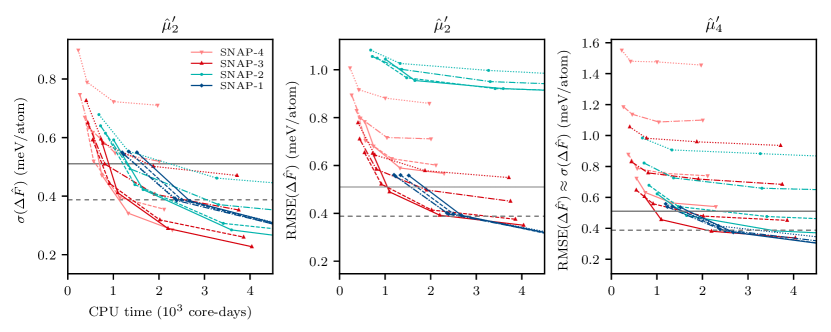
A comparison between the computational times of $\Delta\hat{F}(\hat{\mu}^{\prime}_{2})$ and $\Delta\hat{F}(\hat{\mu}^{\prime}_{4})$ with different approximating potentials $U^{\prime}_{1{}}$ and TDEP of SNAP-0 as $U{{}_{0}}$ is given in Figure 7. The substantial overlap of different lines on each plot, especially on the first one depicting the standard deviation of $\Delta\hat{F}(\hat{\mu}^{\prime}_{2})$, is a good example of what was described above. This indicates that for a given error and computational time there can be several equivalent solutions in terms of chosen $U^{\prime}_{1{}}$, the simulation time and the number of recalculations. For example, it is seen that there is only a slight difference in $\sigma(\Delta\hat{F})$ at around 1000 core-hours of total computational time whether 20 recalculations of 50 ps simulations, 100 recalculations of 10 ps simulations or 10 recalculations of 10 ps simulations at each $\lambda$ are done using SNAP-4, SNAP-2 and SNAP-1 respectively as $U^{\prime}_{1{}}$.

It is also clear that recalculating more energies lowers the standard deviation significantly when $U^{\prime}_{1{}}$ is a bad approximation of $U_{1{}}$, as is the case with SNAP-4, and that there is almost no change except for added computational time with a good approximation, such as SNAP-1. In addition, it is seen that although DFT-4 is about 6 times faster than DFT-1 in MD simulations, it is at best only about 2 times as fast when approximating $\Delta F$ due to the high computational cost of recalculations.

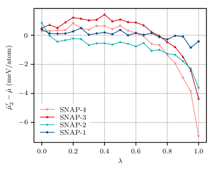
There is a significant change in the results when the bias of $\Delta\hat{F}(\hat{\mu}^{\prime}_{2})$ is taken account in the error, as shown in the second plot of Figure 7. The biases of $\Delta\hat{F}(\hat{\mu}^{\prime}_{2})$ are $0.05$, $-0.8$, $0.3$, $-0.5$ and meV/atom for SNAP-1 to SNAP-4 respectively. It is notable that apart from SNAP-1, the bias seems essentially random. Whereas it could be expected that SNAP-2 is a significantly better approximation of SNAP-0 than SNAP-4, its bias is considerably larger. As shown in Figure 8, this is due to different cancellation of the biases of $\hat{\mu}^{\prime}_{2}$ when integrating over $\lambda$. If instead the error would be defined as $\sqrt{\int_{0}^{1}(\hat{\mu}^{\prime}_{2}-\hat{\mu})^{2}d\lambda}$, the corresponding values would be $0.2$, $1.1$, $1.3$ and $1.7$ meV/atom.

Whether the bias of $\Delta\hat{F}(\hat{\mu}^{\prime}_{2})$ can be considered small enough depends on the application. When free energy differences between different phases are compared, it is possible that the biases either cancel out or add and as shown, the sign of each can depend on the chosen $U^{\prime}_{1{}}$. Furthermore, if the bias is highly non-linear with temperature or volume, it can also have a considerable effect on the derivative properties, such as the heat capacity or thermal expansion coefficient. Therefore in order to obtain accurate results it is best not to rely on the possible cancellation effect which would mean constraining the use of $\Delta\hat{F}(\hat{\mu}^{\prime}_{2})$ to only cases when $U^{\prime}_{1{}}$ is a good approximation of $U_{1{}}$.

Figure 10: Comparison of the RMS error of the different estimators of $F_{1}-F_{1}^{\prime}$ using either cumulant expansion FEP or $\lambda$-switching. In each case the reference potential $U{{}_{0}}$ was TDEP fitted to $U_{1{}}$ and the approximating potential $U^{\prime}_{1{}}$ is given in the title of each subplot. The dotted, dashed-dotted, dashed and solid lines denote simulation times of 10, 20, 50 and 100 ps respectively. $K$ denotes the total number of recalculated structures which in case of $\hat{\mu}^{\prime}_{2}$ and $\hat{\mu}^{\prime}_{4}$ based estimators was divided evenly between 11 equidistant $\lambda$ values.

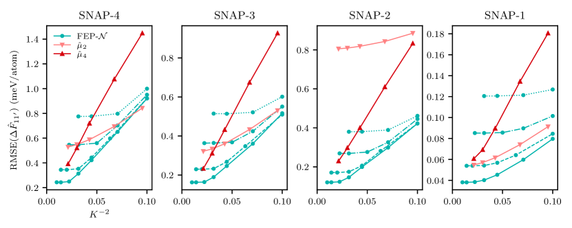
As explained before, another way to avoid biased results is to use $\Delta\hat{F}(\hat{\mu}^{\prime}_{4})$. For the results shown in Figure 7, the bias was typically less than 0.1 meV/atom, therefore $\sigma(\hat{F})$ was very close to $\mathrm{RMSE}(\hat{F})$. The reduced bias comes, however, with the cost of increased variance with an exception when SNAP-1 is used as $U^{\prime}_{1{}}$ as in that case there is essentially no difference between $\Delta\hat{F}(\hat{\mu}^{\prime}_{2})$ and $\Delta\hat{F}(\hat{\mu}^{\prime}_{4})$. This is due to $\operatorname{var}(U_{1{}}-U^{\prime}_{1{}})$ being small enough that essentially for any number of recalculations the error is dominated by $\operatorname{var}(U^{\prime}_{1{}}-U{{}_{0}})$.

III.3 Comparison to FEP

As explained in Section II.1, the correction term

$$\hat{\mu}^{\prime}_{c}(\lambda)=\int_{0}^{1}\left[\hat{\mu}^{\prime}(\lambda)-\frac{1}{N}\displaystyle\sum_{i=1}^{N}\left(U^{\prime}_{1{i}}-U{{}_{0}}{{}_{i}}\right)_{\lambda^{\prime}}\right]d\lambda$$ (27)

with $\hat{\mu}^{\prime}$ being either $\hat{\mu}^{\prime}_{2}$ of $\hat{\mu}^{\prime}_{4}$, estimates the free energy difference $\Delta F_{11^{\prime}}=F_{1}-F_{1}^{\prime}$. Since both of the estimators depend on the reference potential $U{{}_{0}}$ (it does not appear explicitly in the correction term when using $\hat{\mu}^{\prime}_{2}$, but is included in the potential $U^{\prime}$ that is used for sampling), so do the bias and variance of the estimated $\Delta F_{11^{\prime}}$ which in turn propagates to the error of $\Delta\hat{F}$.

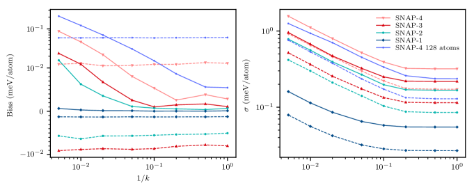
Free energy perturbation provides a more natural way of estimating $\Delta F_{11^{\prime}}$ such that its error does not depend on $U{{}_{0}}$, but only on the distribution of $U_{1{}}-U^{\prime}_{1{}}$ sampled at $\lambda=1$. As the results in Figure 9 show, when using either $\Delta\hat{F}_{11^{\prime}}$ or $\Delta\hat{F}_{11^{\prime},\mathcal{N}}$ the uncertainty of the results in all cases is dominated by the standard deviation instead of bias with the latter being approximately an order of magnitude smaller. This can be attributed mainly to the small system size which limits $\operatorname{var}[\beta(U_{1{}}-U^{\prime}_{1{}})]$ to reasonably small values (1.4 with 54 and 3.3 with 128 atoms) even for the worst $U^{\prime}_{1{}}$ . The bias of $\Delta\hat{F}_{11^{\prime},\mathcal{N}}$ does not depend significantly on the number of recalculated energies, which is expected since the sample variance is an unbiased estimator of the population variance. The value of the bias, although not zero, which indicates that the distribution of $U_{1{}}-U^{\prime}_{1{}}$ is not perfectly Gaussian, is nevertheless small enough that it can be considered negligible and $\Delta\hat{F}_{11^{\prime},\mathcal{N}}$ is therefore a good approximation for the potentials used in this work. The main advantage of $\Delta\hat{F}_{11^{\prime},\mathcal{N}}$ compared to $\Delta\hat{F}_{11^{\prime}}$ is the approximately two times decrease in the standard deviation of the estimated free energy difference. Given uncorrelated samples, about four times fewer calculations would be needed to reach the same uncertainty, however, the improvement can be even higher as evident by the leveling off of the decrease in $\sigma$ when more than 10-20% energies are recalculated.

The latter also means that given some fixed number of samples at each $\lambda$ that is needed to converge the uncorrected free energy difference $F_{1}^{\prime}-F_{0}$ (Equation 20), it is possible that using FEP might not be as efficient for estimating $F_{1}-F_{1}^{\prime}$ compared to Equation 27. Assuming that each recalculated energy provides certain constant amount of information about $F_{1}-F_{1}^{\prime}$, then instead of recalculating, for example, 5% of energies at 10 values of $\lambda$ when calculating $\Delta\hat{F}(\hat{\mu}^{\prime}_{2})$ or $\Delta\hat{F}(\hat{\mu}^{\prime}_{4})$, with FEP $10\cdot 5=50\%$ energies would have to be recalculated in order to get the same uncertainty. If that fraction of energies is greater than the threshold above which the correlations between samples become large enough, there is no reduction in the overall uncertainty.

In practice, the comparison is more complicated mainly because each recalculated sample does not necessarily provide the same amount of information. It can expected that with $\Delta\hat{F}(\hat{\mu}^{\prime}_{2})$ and $\Delta\hat{F}(\hat{\mu}^{\prime}_{4})$ either recalculating different number of energies at each $\lambda$ or assigning different weights to each $\hat{\mu}$ when fitting the polynomial could result in slightly better $\sigma(\Delta\hat{F})$. Whereas this was not as crucial for the results in the previous sections since the comparison was between methods that used the same data, this is not the case when estimating $\Delta F_{11^{\prime}}$ using FEP. Consequently a full analysis would deserve a separate study and the results presented here are only for the case when neither the length of the simulation nor the number of recalculated energies do not depend on $\lambda$ and the comparison will only be made for estimating $F_{1}-F_{1}^{\prime}$, not $F_{1}-F_{0}$.

The results in Figure 10 illustrate what was pointed out above. FEP-$\mathcal{N}$can have larger error when estimating $F_{1}-F_{1}^{\prime}$ compared to $\hat{\mu}^{\prime}_{2}$ or $\hat{\mu}^{\prime}_{4}$ for short simulation times as the decrease in variance due to added number of recalculations will be limited due to time correlations. For longer simulation times, in which case both $\hat{\mu}$-based estimators and FEP-$\mathcal{N}$make use of only uncorrelated data, the latter is more efficient and has smaller error. In other words, at least for the given potentials and system size, FEP-$\mathcal{N}$makes better use of the recalculated energies given that those are randomly sampled. FEP, however, is not necessarily better due to significantly larger variance.

III.4 Comparisons of $\hat{\mu}^{\prime}_{1}$ to $\hat{\mu}^{\prime}_{2}$ and $\hat{\mu}^{\prime}_{3}$ to $\hat{\mu}^{\prime}_{4}$

Figure 11: Ratio of the standard deviations of the free energy estimators based on either all of the available data or only those of the recalculated timesteps. The solid lines correspond to $a=3$, $b=4$ and the dashed lines to $a=1$, $b=2$. Values below 1 indicate the cases when using the free energy estimator based on fewer data results in lower standard deviation. $1/k$ is the fraction of the number of recalculated energies.

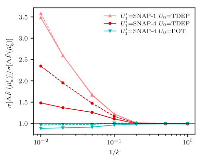
The estimators of $\Delta F$ presented so far have been based on either $\hat{\mu}^{\prime}_{2}$ and $\hat{\mu}^{\prime}_{4}$ and not $\hat{\mu}^{\prime}_{1}$ or $\hat{\mu}^{\prime}_{3}$, i.e. the variants that only incorporate energy differences corresponding to the recalculated timesteps. It would be natural to expect that using fewer samples would result in increased standard deviation, which is the case for a regular sample mean, but as shown in Figure 11 this is not necessarily the case. The results show that among the combinations of $U^{\prime}_{1{}}$ and $U{{}_{0}}$ considered in this study, the standard deviation can indeed increase significantly, but also decrease. Because those cases are not in any way guaranteed to form a representative sample and do not explain the magnitude and the direction of the change in the standard deviation, it is worthwhile to investigate it theoretically. For simplicity, only the comparison between $\hat{\mu}^{\prime}_{1}$ and $\hat{\mu}^{\prime}_{2}$ is given.

If three sample means are defined as

$$\hat{m}_{1} =\frac{k}{N}\sum_{i=1}^{N/k}\left(U^{\prime}_{1{{ki}}}-U_{0}{{}_{ki}}\right)_{\lambda^{\prime}}$$ (28a)

$$\hat{m}_{2} =\frac{k}{N}\sum_{i=1}^{N/k}\left(U_{1{}}{{}_{ki}}-U^{\prime}_{1{{ki}}}\right)_{\lambda^{\prime}}$$ (28b)

$$\hat{m}_{3} =\frac{1}{N}\sum_{i=1}^{N}\left(U^{\prime}_{1{{i}}}-U_{0}{{}_{i}}\right)_{\lambda^{\prime}}$$ (28c)

then $\hat{\mu}^{\prime}_{1}$ and $\hat{\mu}^{\prime}_{2}$ can be written as

$$\hat{\mu}^{\prime}_{1} =\hat{m}_{1}+\hat{m}_{2}$$ (29a)

$$\hat{\mu}^{\prime}_{2} =\hat{m}_{3}+\hat{m}_{2}$$ (29b)

Although the $N$ samples in Equation 28c are usually correlated, assuming that they are random does not qualitatively change the results and in that case

$$\operatorname{var}(\hat{m}_{1})=k\operatorname{var}(\hat{m}_{3})$$ (30)

Then by defining $\gamma$ and $\rho$ as

$$\operatorname{var}(\hat{m}_{1}) =\gamma\operatorname{var}(\hat{m}_{2})$$ (31a)

$$\rho =\operatorname{corr}(\hat{m}_{1},\hat{m}_{2})$$ (31b)

it can be shown that

$$\frac{\operatorname{var}(\hat{\mu}^{\prime}_{1})}{\operatorname{var}(\hat{\mu}^{\prime}_{2})}=\eta(\rho,\gamma,k)=\frac{\gamma+2\rho\sqrt{\gamma}+1}{\gamma/k+2\rho\sqrt{\gamma}/k+1}$$ (32)

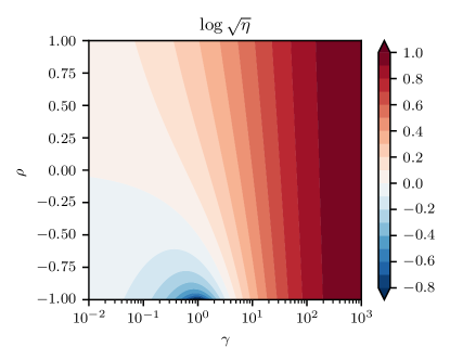
The values of this function at fixed $k=100$ are shown in Figure 12. Irrespective of the value of $k$, the condition for $\eta<1$, i.e. that using fewer samples results in smaller variance, is

$$\rho\leq-\frac{\sqrt{\gamma}}{2}$$ (33)

Which means that in addition to $\rho$ being negative the value of $\gamma$ can be at most 4.

Since

$$\operatorname{var}(\hat{m}_{1}) =k/N\operatorname{var}\left(U{{}_{0}}-U^{\prime}_{1{}}\right)$$ (34a)

$$\operatorname{var}(\hat{m}_{2}) =k/N\operatorname{var}\left(U_{1{}}-U^{\prime}_{1{}}\right)$$ (34b)

then $\gamma$ can also be written as

$$\gamma=\frac{\operatorname{var}\left(U{{}_{0}}-U^{\prime}_{1{}}\right)}{\operatorname{var}\left(U_{1{}}-U^{\prime}_{1{}}\right)}$$ (35)

and using similar reasoning

$$\rho=\operatorname{corr}(U^{\prime}_{1{}}-U{{}_{0}},U_{1{}}-U^{\prime}_{1{}})$$ (36)

This suffices to explain the results in Figure 11. Since typically $U{{}_{0}}$ does not approximate $U^{\prime}_{1{}}$ as well as $U_{1{}}$, $\gamma\gg 1$ and it is better to use $\hat{\mu}^{\prime}_{2}$ over $\hat{\mu}^{\prime}_{1}$. This is observed for both cases when TDEP was used as the reference potential. With SNAP-1 as $U^{\prime}_{1{}}$, $\eta$ is larger due to the variance of $U_{1{}}-U^{\prime}_{1{}}$ being significantly smaller. At the limit of infinite $\gamma$, $\eta$ approaches $k$.

At $\gamma=1$ and $\rho=-1$, for example when $U{{}_{0}}=U_{1{}}$, $\eta$ becomes zero. SNAP as a reference potential, although not perfect, is able to get closer to that point compared to TDEP, in this case on average over all $\lambda$ values $\gamma=1.8$ and $\rho=-0.71$. This satisfies Equation 33 which results in $\Delta\hat{F}(\hat{\mu}^{\prime}_{1})$ having slightly lower variance than $\Delta\hat{F}(\hat{\mu}^{\prime}_{2})$. Whereas not investigated here, it must be noted that as $U{{}_{0}}$ approaches $U_{1{}}$, the need for using $U^{\prime}_{1{}}$ disappears, since it likely becomes better to estimate $F_{1}-F_{0}$ directly by FEP or FEP-$\mathcal{N}$.

Figure 12: Dependence of $\eta$ on $\gamma$ and $\rho$ at $k=100$. Region where $\eta<1$ indicates conditions when using fewer data, i.e. $\hat{\mu}^{\prime}_{1}$ instead of $\hat{\mu}^{\prime}_{2}$, results in smaller variance.

IV Conclusions

Even though only a single atomic system was investigated and the numerical calculations were performed using SNA potentials fitted to DFT instead of the latter directly, the results nevertheless provide insight into the possible issues and pitfalls when employing different correction schemes for estimating converged free energy differences from non-converged DFT-MD simulations.

The choice between estimating the free energy difference between a target and a reference system either by using the UP-TILD method ($\Delta\hat{F}(\hat{\mu}^{\prime}_{2})$) or by weighted ensemble averages ($\Delta\hat{F}(\hat{\mu}^{\prime}_{4})$) determines whether the error of the results is dominated by bias, as is the case for the former method, or by variance as is the case for the latter. As opposed to $\Delta\hat{F}(\hat{\mu}^{\prime}_{4})$, the bias of $\Delta\hat{F}(\hat{\mu}^{\prime}_{2})$ cannot be reduced by longer simulations or by recalculating a larger number of energies using the converged potential $U_{1{}}$. This limits the choice of both the reference ($U{{}_{0}}$) and the approximating ($U^{\prime}_{1{}}$) potentials, which have to be relatively close approximations of $U_{1{}}$. Most importantly, fitting $U{{}_{0}}$ to $U^{\prime}_{1{}}$ instead of $U_{1{}}$ can significantly increase the bias, in some cases by more than an order of magnitude, and should therefore be avoided. In addition, an anharmonic $U{{}_{0}}$ is substantially better than a harmonic one both for reducing the bias and the variance of either estimator. Whereas this complicates the analysis, since the free energy of the reference system has to be calculated separately, for a given computational time it allows for much more accurate and precise results.

As opposed to $\Delta\hat{F}(\hat{\mu}^{\prime}_{2})$, $\Delta\hat{F}(\hat{\mu}^{\prime}_{4})$ could estimate $\Delta F$ accurately even using the worst $U^{\prime}_{1{}}$ and $U{{}_{0}}$. For the combinations of potentials, simulation times and the number of recalculated energies considered in this paper, the bias of $\Delta\hat{F}(\hat{\mu}^{\prime}_{4})$ did not pose a problem since the variance of it was significantly larger. Therefore, by minimizing the variance to an acceptable level, the bias was reduced to be insignificant. However, the variance was in every case larger than that of $\Delta\hat{F}(\hat{\mu}^{\prime}_{2})$, which requires longer simulations and more recalculations in order to achieve the same precision.

Choosing an optimal $U^{\prime}_{1{}}$ can be difficult. Using a bad approximation results in faster MD simulations, but due to the increased variance more recalculated energies are needed and for a given target precision the total computational time can be longer compared to when a better $U^{\prime}_{1{}}$ is used. Since poor $U^{\prime}_{1{}}$ can also significantly increase the bias of $\Delta\hat{F}(\hat{\mu}^{\prime}_{2})$ or the variance of $\Delta\hat{F}(\hat{\mu}^{\prime}_{4})$, although possibly not the optimal one, a relatively safe choice is DFT with only a slightly reduced convergence parameters.

Both of the correction schemes estimate $F_{1}-F_{1}^{\prime}$, i.e. the free energy difference between systems with converged and non-converged potentials. As opposed to the direct thermodynamic path, this is done on a path between the non-converged potential to the reference. Therefore the estimated $F_{1}-F_{1}^{\prime}$ depends on $U{{}_{0}}$ whereas the actual free energy difference does not. This can reduce the efficiency and accuracy compared to a direct FEP estimate. However, as the results show, FEP is not necessarily better in every case. The main reason behind this is that distributing the recalculated energies among all the $\lambda$-values can result in a larger amount of uncorrelated samples than doing it at only $\lambda=1$, as is the case with FEP. On the other hand, even with the worst $U^{\prime}_{1{}}$, the bias did not pose a problem neither with FEP nor its cumulant expansion approximation.

Finally, for both $\Delta\hat{F}(\hat{\mu}^{\prime}_{2})$ and $\Delta\hat{F}(\hat{\mu}^{\prime}_{4})$ there are corresponding estimators that as opposed to all of the MD data, only use that which corresponds to the recalculated timesteps. Whereas in general using more data results in smaller variance, in some cases, namely when using a good reference potential, the opposite can be true.

V Acknowledgments

The research leading to these results has been partially funded by the Swedish Centre for Nuclear Technology (SKC). Computational resources were provided by Swedish National Infrastructure for Computing (SNIC).

References

- Bendick and Pepperhoff [1982] W. Bendick and W. Pepperhoff, On the / phase stability of iron, Acta Metallurgica 30, 679 (1982).
- Dinsdale [1991] A. T. Dinsdale, SGTE data for pure elements, Calphad 15, 317 (1991).
- Grabowski et al. [2011] B. Grabowski, P. Söderlind, T. Hickel, and J. Neugebauer, Temperature-driven phase transitions from first principles including all relevant excitations: The fcc-to-bcc transition in Ca, Physical Review B - Condensed Matter and Materials Physics 84, 214107 (2011).
- Burke [2012] K. Burke, Perspective on density functional theory, Journal of Chemical Physics 136, 150901 (2012).
- Jones [2015] R. O. Jones, Density functional theory: Its origins, rise to prominence, and future, Reviews of Modern Physics 87, 10.1103/RevModPhys.87.897 (2015).
- Palumbo et al. [2014] M. Palumbo, B. Burton, A. Costa e silva, B. Fultz, B. Grabowski, G. Grimvall, B. Hallstedt, O. Hellman, B. Lindahl, A. Schneider, P. E. Turchi, and W. Xiong, Thermodynamic modelling of crystalline unary phases, Physica Status Solidi (B) Basic Research 251, 14 (2014).
- Moustafa et al. [2017] S. G. Moustafa, A. J. Schultz, E. Zurek, and D. A. Kofke, Accurate and precise ab initio anharmonic free-energy calculations for metallic crystals: Application to hcp Fe at high temperature and pressure, Physical Review B 96, 014117 (2017).
- Wagner et al. [1998] F. Wagner, T. Laloyaux, and M. Scheffler, Errors in Hellmann-Feynman forces due to occupation-number broadening and how they can be corrected, Physical Review B - Condensed Matter and Materials Physics 57, 2102 (1998).
- Kratzer and Neugebauer [2019] P. Kratzer and J. Neugebauer, The basics of electronic structure theory for periodic systems, Frontiers in Chemistry 7, 1 (2019).
- Dove [2011] M. Dove, Introduction to the theory of lattice dynamics, École thématique de la Société Française de la Neutronique 12, 123 (2011).
- Togo and Tanaka [2015] A. Togo and I. Tanaka, First principles phonon calculations in materials science, Scripta Materialia 108, 1 (2015).
- Frenkel and Smit [2002] D. Frenkel and B. Smit, Understanding Molecular Simulation (Academic Press, San Diego, 2002).
- Rickman and LeSar [2002] J. M. Rickman and R. LeSar, Free-energy calculations in materials research, Annual Review of Materials Science 32, 195 (2002).
- Chipot and Pohorille [2007] C. Chipot and A. Pohorille, Calculating Free Energy Differences Using Perturbation Theory, in Free Energy Calculations, Vol. 86, edited by A. Pohorille and C. Chipot (Springer, Berlin, Heidelberg, 2007) Chap. 2, pp. 33–75.
- Vočadlo and Alfè [2002] L. Vočadlo and D. Alfè, Ab initio melting curve of the fcc phase of aluminum, Physical Review B - Condensed Matter and Materials Physics 65, 1 (2002).
- Grabowski et al. [2009] B. Grabowski, L. Ismer, T. Hickel, and J. Neugebauer, Ab initio up to the melting point: Anharmonicity and vacancies in aluminum, Physical Review B - Condensed Matter and Materials Physics 79, 134106 (2009).
- Duff et al. [2015] A. I. Duff, T. Davey, D. Korbmacher, A. Glensk, B. Grabowski, J. Neugebauer, and M. W. Finnis, Improved method of calculating ab initio high-temperature thermodynamic properties with application to ZrC, Physical Review B - Condensed Matter and Materials Physics 91, 214311 (2015).
- Sun et al. [2018] T. Sun, J. P. Brodholt, Y. Li, and L. Vočadlo, Melting properties from ab initio free energy calculations: Iron at the Earth’s inner-core boundary, Physical Review B 98, 1 (2018).
- Rang and Kresse [2019] M. Rang and G. Kresse, First-principles study of the melting temperature of MgO, Physical Review B 99, 184103 (2019).
- Frenkel and Ladd [1984] D. Frenkel and A. J. Ladd, New Monte Carlo method to compute the free energy of arbitrary solids. Application to the fcc and hcp phases of hard spheres, The Journal of Chemical Physics 81, 3188 (1984).
- Kirkwood [1935] J. G. Kirkwood, Statistical Mechanics of Fluid Mixtures, The Journal of Chemical Physics 3, 300 (1935).
- Wood et al. [1991] R. H. Wood, W. C. F. Muhlbauer, and P. T. Thompson, Systematic errors in free energy perturbation calculations due to a finite sample of configuration space: sample-size hysteresis, The Journal of Physical Chemistry 95, 6670 (1991).
- Zuckerman and Woolf [2002] D. M. Zuckerman and T. B. Woolf, Theory of a Systematic Computational Error in Free Energy Differences, Physical Review Letters 89, 180602 (2002).
- Gore et al. [2003] J. Gore, F. Ritort, and C. Bustamante, Bias and error in estimates of equilibrium free-energy differences from nonequilibrium measurements, Proceedings of the National Academy of Sciences 100, 12564 (2003).
- Zuckerman and Woolf [2004] D. M. Zuckerman and T. B. Woolf, Systematic Finite-Sampling Inaccuracy in Free Energy Differences and Other Nonlinear Quantities, Journal of Statistical Physics 114, 1303 (2004).
- Wu and Kofke [2004] D. Wu and D. A. Kofke, Model for small-sample bias of free-energy calculations applied to Gaussian-distributed nonequilibrium work measurements, The Journal of Chemical Physics 121, 8742 (2004).
- Wu and Kofke [2005] D. Wu and D. A. Kofke, Phase-space overlap measures. I. Fail-safe bias detection in free energies calculated by molecular simulation, Journal of Chemical Physics 123, 10.1063/1.1992483 (2005).
- Jarzynski [2006] C. Jarzynski, Rare events and the convergence of exponentially averaged work values, Physical Review E 73, 046105 (2006).
- Pohorille et al. [2010] A. Pohorille, C. Jarzynski, and C. Chipot, Good practices in free-energy calculations, Journal of Physical Chemistry B 114, 10235 (2010).
- Boresch and Woodcock [2017] S. Boresch and H. L. Woodcock, Convergence of single-step free energy perturbation, Molecular Physics 115, 1200 (2017).
- Wood and Thompson [2018] M. A. Wood and A. P. Thompson, Extending the accuracy of the SNAP interatomic potential form, The Journal of Chemical Physics 148, 241721 (2018).
- Shyu and Ytreberg [2009] C. Shyu and F. M. Ytreberg, Reducing the bias and uncertainty of free energy estimates by using regression to fit thermodynamic integration data, Journal of Computational Chemistry , NA (2009).
- Jorge et al. [2010] M. Jorge, N. M. Garrido, A. J. Queimada, I. G. Economou, and E. A. MacEdo, Effect of the integration method on the accuracy and computational efficiency of free energy calculations using thermodynamic integration, Journal of Chemical Theory and Computation 6, 1018 (2010).
- Ryde [2017] U. Ryde, How Many Conformations Need to Be Sampled to Obtain Converged QM/MM Energies? the Curse of Exponential Averaging, Journal of Chemical Theory and Computation 13, 5745 (2017).
- Hellman [2012] O. Hellman, Thermal properties of materials from first principles, Ph.D. thesis, Linköping University (2012).
- Efron [1979] B. Efron, Bootstrap Methods: Another Look at the Jackknife, The Annals of Statistics 7, 1100 (1979).
- Kresse and Hafner [1993] G. Kresse and J. Hafner, Ab initio molecular dynamics for liquid metals, Physical Review B 47 (1993).
- Kresse and Hafner [1994] G. Kresse and J. Hafner, Ab initio molecular-dynamics simulation of the liquid-metal-amorphous-semiconductor transition in germanium, Phys. Rev. B 49, 14251 (1994).
- Kresse and Furthmuller [1996] G. Kresse and J. Furthmuller, Efficiency of ab-initio total energy calculations for metals and semiconductors using a plane-wave basis set, Comp. Mater. Sci. 6, 15 (1996).
- Kresse and Furthmüller [1996] G. Kresse and J. Furthmüller, Efficient iterative schemes for ab initio total-energy calculations using a plane-wave basis set., Physical review. B, Condensed matter 54, 11169 (1996).
- Kresse and Joubert [1999] G. Kresse and D. Joubert, From ultrasoft pseudopotentials to the projector augmented-wave method, Phys. Rev. B 59, 1758 (1999).
- [42] FitSNAP. https://github.com/FitSNAP/FitSNAP.
- Hellman et al. [2011] O. Hellman, I. A. Abrikosov, and S. I. Simak, Lattice dynamics of anharmonic solids from first principles, Physical Review B 84, 180301(R) (2011).
- Thompson et al. [2015] A. Thompson, L. Swiler, C. Trott, S. Foiles, and G. Tucker, Spectral neighbor analysis method for automated generation of quantum-accurate interatomic potentials, Journal of Computational Physics 285, 316 (2015).
- Plimpton [1995] S. Plimpton, Fast Parallel Algorithms for Short-Range Molecular Dynamics, Journal of Computational Physics 117, 1 (1995).
- Ceriotti et al. [2009] M. Ceriotti, G. Bussi, and M. Parrinello, Langevin equation with colored noise for constant-temperature molecular dynamics simulations, Physical Review Letters 102, 1 (2009).
- Ceriotti et al. [2010] M. Ceriotti, G. Bussi, and M. Parrinello, Colored-Noise Thermostats à la Carte, Journal of Chemical Theory and Computation 6, 1170 (2010).