22email: nanliu4@illinois.edu, {lishuang,yilundu,torralba,jbt}@mit.edu
Compositional Visual Generation with
Composable Diffusion Models
Abstract
Large text-guided diffusion models, such as DALL-E 2, are able to generate stunning photorealistic images given natural language descriptions. While such models are highly flexible, they struggle to understand the composition of certain concepts, such as confusing the attributes of different objects or relations between objects. In this paper, we propose an alternative structured approach for compositional generation using diffusion models. An image is generated by composing a set of diffusion models, with each of them modeling a certain component of the image. To do this, we interpret diffusion models as energy-based models in which the data distributions defined by the energy functions may be explicitly combined. The proposed method can generate scenes at test time that are substantially more complex than those seen in training, composing sentence descriptions, object relations, human facial attributes, and even generalizing to new combinations that are rarely seen in the real world. We further illustrate how our approach may be used to compose pre-trained text-guided diffusion models and generate photorealistic images containing all the details described in the input descriptions, including the binding of certain object attributes that have been shown difficult for DALL-E 2. These results point to the effectiveness of the proposed method in promoting structured generalization for visual generation. ††footnotetext: Webpage: https://energy-based-model.github.io/Compositional-Visual-Generation-with-Composable-Diffusion-Models/
Keywords:
Compositionality, Diffusion Models, Energy-based Models, Visual Generation1 Introduction
Our understanding of the world is highly compositional in nature. We are able to rapidly understand new objects from their components, or compose words into complex sentences to describe the world states we encounter [26]. We are able to make “infinite use of finite means” [4], i.e., repeatedly reuse and recombine concepts we have acquired in a potentially infinite manner. We are interested in constructing machine learning systems to have such compositional capabilities, particularly in the context of generative modeling.
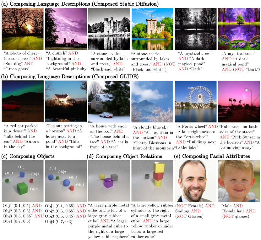
Existing text-conditioned diffusion models such as DALL-E 2 [39] have recently made remarkable strides towards compositional generation, and are capable of generating photorealistic images given textual descriptions. However, such systems are not fully compositional and generate incorrect images when given more complex descriptions [31, 49]. An underlying difficulty may be that such models encode text descriptions as fixed-size latent vectors. However, as textual descriptions become more complex, more information needs to be squeezed into the fixed-size vector. Thus it is impossible to encode arbitrarily complex textual descriptions.
In this work, we propose to factorize the compositional generation problem, using different diffusion models to capture different subsets of a compositional specification. These diffusion models are then explicitly composed together to generate an image. By explicitly factorizing the compositional generative modeling problem, our method can generalize to significantly more complex combinations that are unseen during training.
Such an explicit form of compositionality has been explored before under the context of Energy-Based Models (EBMs) [7, 8, 28]. However, directly training EBMs has been proved to be unstable and hard to scale. We show that diffusion models can be interpreted as implicitly parameterized EBMs, which can be further composed for image generation, significantly improving training stability and image quality.
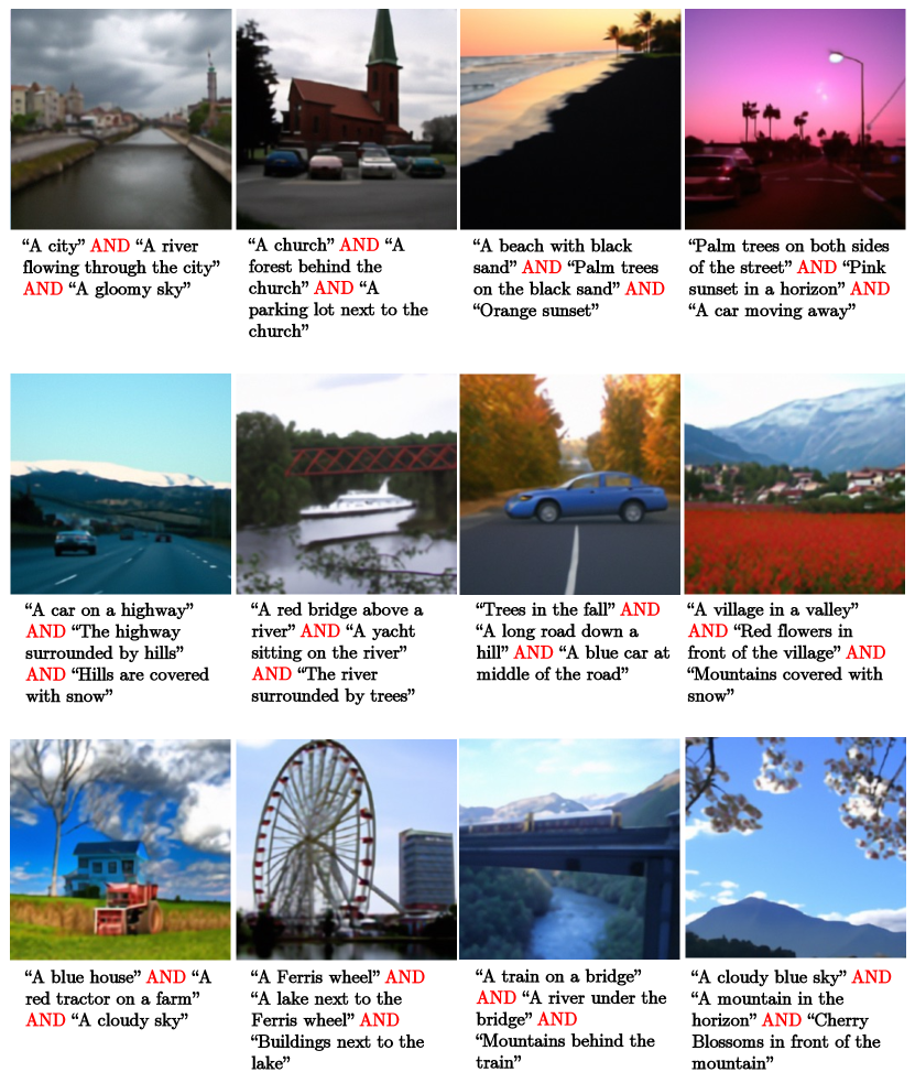
Our proposed method enables zero-shot compositional generation across different domains as shown in Figure 1. First, we illustrate how our approach may be applied to large pre-trained diffusion models, such as Stable Diffusion [42] and GLIDE [33], to compose multiple text descriptions. Next, we illustrate how our approach can be applied to compose objects and object relations, enabling zero-shot generalization to a larger number of objects. Finally, we illustrate how our framework can compose different facial attributes to generate human faces.
Contributions: In this paper, we introduce an approach towards compositional visual generation using diffusion models. First, we show that diffusion models can be composed by interpreting them as energy-based models, and drawing on this connection, we demonstrate how to compose diffusion models together. Second, we propose two compositional operators, Conjunction and Negation, on top of diffusion models that allow us to compose concepts in different domains during inference without any additional training. We show that the proposed method enables effective zero-shot combinatorial generalization, i.e. generating images with more complicated compositions of concepts. Finally, we evaluate our method on composing language descriptions, objects, object relations, and human facial attributes. Our method can generate high-quality images containing all the concepts and outperforms baselines by a large margin. For example, the accuracy of our method is higher than the best baseline for composing three objects in specified positions on the CLEVR dataset.
2 Related Work
Controllable Image Generation. Our work is related to existing work on controllable image generation. One type of approach towards controllable image generation specifies the underlying content of an image utilizing text through GANs [53, 54, 2], VQ-VAEs [40], or diffusion models [33]. An alternative type of approach towards controllable image generation manipulates the underlying attributes in an image [45, 52, 56]. In contrast, we are interested in compositionally controlling the underlying content of an image at test time, generating images that exhibit compositions of multiple types of image content. Thus, most relevant to our work, existing work has utilized EBMs to compose different factors describing a scene [7, 36, 8, 28]. We illustrate how we may implement such probabilistic composition on diffusion models, achieving better performance.
Diffusion Models. Diffusion models have emerged as a promising class of generative models that formulates the data-generating process as an iterative denoising procedure [46, 15]. The denoising procedure can be seen as parameterizing the gradients of the data distribution [48], which is similar to EBMs [27, 10, 37, 12, 11]. Diffusion models have recently shown great promise in image generation tasks [6], enabling effective image editing [32, 24], text conditioning [33, 41, 13], and image inpainting [43]. The iterative, gradient-based sampling of diffusion models enable us to compose multiple factors during inference. While diffusion models have been developed for image generation [47], they have further proven successful in the generation of waveforms [3], 3D shapes [55], decision making [18], and text [1], suggesting that our proposed composition operators may further be applied in such domains.
3 Background
3.1 Denoising Diffusion Models
Denoising Diffusion Probabilistic Models (DDPMs) are a class of generative models where generation is modeled as a denoising process. Starting from a sampled noise, the diffusion model performs denoising steps until a sharp image is formed. In particular, the denoising process produces a series of intermediate images with decreasing levels of noise, denoted as , where is sampled from a Gaussian prior and is the final output image.
DDPMs construct a forward diffusion process by gradually adding Gaussian noise to the ground truth image. A diffusion model then learns to revert this noise corruption process. Both the forward processes and the reverse process are modeled as the products of Markov transition probabilities:
| (1) |
where is the real data distribution and is a standard Gaussian prior.
A generative process is trained to generate realistic images by approximating the reverse process through variational inference. Each step of the generative process is a Gaussian distribution with a learned mean and covariance matrix , where is the identity matrix.
| (2) |
The mean is represented by a perturbation to a noisy image . The goal is to remove the noise gradually by predicting a less noisy image at timestep given a noisy image . To generate real images, we sample from to using the parameterized marginal distribution , with an individual step corresponding to:
| (3) |
The generated images become more realistic over multiple iterations.
3.2 Energy Based Models
Energy-Based Models (EBMs) [10, 9, 12, 37] are a class of generative models where the data distribution is modeled using an unnormalized probability density. Given an image , the probability density of image is defined as:
| (4) |
where the energy function is a learnable neural network. A gradient based MCMC procedure, Langevin dynamics [10], is then used to sample from the unnormalized probability distribution to iteratively refine the generated image :
| (5) |
The sampling procedure used by diffusion models in Equation (3) is functionally similar to the sampling procedure used by EBMs in Equation (5). In both settings, images are iteratively refined starting from a Gaussian noise, with a small amount of additional noise added at each iterative step.

4 Our approach
In this section, we first introduce how we interpret diffusion models as energy-based models in section 4.1 and then introduce how we compose diffusion models for visual generation in section 4.2.
4.1 Diffusion Models as Energy Based Models
The sampling procedure of diffusion models in Equation (3) and EBMs in Equation (5) are functionally similar. At a timestep , in diffusion models, images are updated using a learned denoising network while in EBMs, images are updated using the gradient of the energy function . The denoising network is trained to predict the underlying score of the data distribution [51, 47] when the number of diffusion steps increases to infinity. Similarly, an EBM is trained so that corresponds to the score of the data distribution as well. In this sense, and are functionally the same, and the underlying sampling procedure in Equation (3) and Equation (5) are equivalent. We may view a trained diffusion model as an implicitly parameterized EBM. Such parameterization enables us to apply previous techniques for composing EBMs to diffusion models.
Composing EBMs. Previous EBMs [14, 7, 28] have shown good performance on compositional visual generation. Given independent EBMs, , the functional form of EBMs in Equation (4) enables us to compose multiple separate EBMs together to obtain a new EBM. The composed distribution can be represented as:
| (6) |
where is the probability density of image (Equation (4)). Langevin dynamics is then used to iteratively refine the generated image [7, 28].
| (7) |
Composing Diffusion Models. By leveraging the interpretation that diffusion models are functionally similar to EBMs, we may compose diffusion models in a similar way. The generative process and the score function of a diffusion model can be represented as and , respectively. If we treat the score functions in diffusion models as the learned gradient of energy functions in EBMs, the score function of the composed diffusion model can be written as . Thus the generative process of composing multiple diffusion models becomes:
| (8) |
A complication of parameterizing a gradient field of EBM with a learned score function is that the gradient field may not be conservative, and thus does not correspond to a valid probability density. However, as discussed in [44], explicitly parameterizing the learned function as the gradient of EBM achieves similar performance as the non-conservative parameterization of diffusion models, suggesting this is not problematic.
4.2 Compositional Generation through Diffusion Models
Next, we discuss how we compose diffusion models for image generation. We aim to generate images conditioned on a set of concepts . To do this, we represent each concept using a diffusion model, which can be composed to generate images. Inspired by EBMs [7, 28], we define two compositional operators, conjunction (AND) and negation (NOT), to compose diffusion models. We learn a set of diffusion models representing the conditional probability distribution given concept and an unconditional probability distribution .
Concept Conjunction (AND). We aim to generate images containing certain attributes. Following [7], the conditional probability can be factorized as:
| (9) |
Here we assume the concepts are conditionally independent given . We can represent using the combination of a conditional distribution and an unconditional distribution , with both of them are parameterized as diffusion models . The expression of corresponds to the implicit classifier that represents the likelihood of exhibiting concept . Substituting in Equation 9, we can rewrite Equation 9 as:
| (10) |
We sample from this resultant distribution using Equation (8) with the composed score function :
| (11) |
where is a hyperparameter corresponding to the temperature scaling on concept . We can generate images with the composed concepts using the following generative process:
| (12) |
In the setting in which image generation is conditioned on a single concept, the above sampling procedure reduces to the classifier-free guidance [16].
Concept Negation (NOT). In concept negation, we aim to generate realistic images with the absence of a certain factor . However, the negation of a concept can be ill-defined. For example, the negation of “dark” can be “bright” or random noises. Thus we generate images conditioned other concepts as well to make the generated images look real. Following [7], concept negation can be represented as the composed probability distribution . Similarly, we refactorize the joint probability distribution as:
| (13) |
Using the factorization , we can rewrite Equation (13) as:
| (14) |
We may construct the composed score funcion as:
| (15) |
where is the hyperparameter that controls the strength of the negation. We can generate samples using this composed score function and Equation 12.
Algorithm 1 provides the pseudo-code for composing diffusion models using concept conjunction and negation. Our method can compose pre-trained diffusion models during inference without any additional training. Please see the full derivation details for both operators in appendix 0.F.
5 Experiment Setup
5.1 Datasets
CLEVR. CLEVR [19] is a synthetic dataset containing objects with different shapes, colors, and sizes. The training set consists of 30,000 images at resolution. Each image contains objects and a 2D coordinate label indicating that the image contains an object at . In our experiments, the 2D coordinate label is the coordinate of one object in the image.
Relational CLEVR. Relational CLEVR [28] contains relational descriptions between objects in the image, such as “a red cube to the left of a blue cylinder”. The training dataset contains images at resolution. Each training image contains objects and one label describing a relation between two objects. If there is only one object in the image, the second object and their relation in the relational description are both nulls.
FFHQ. FFHQ [22] is a real-world human face dataset. The original FFHQ dataset consists of 70,000 human face images without labels. [5] annotates three binary attributes, including smile, gender, and glasses, for the images using pre-trained classifiers. In total, there are 51,067 images labeled by the classifiers.
5.2 Evaluation Metrics
Binary classification accuracy. During testing, we evaluate the performance of the proposed method and baselines on three different settings. The first test setting, 1 Component, generates images conditioned on a single concept (matching the training distribution). The second and third test settings, 2 Components and 3 Components, generate images by composing two and three concepts, respectively, using the conjunction and negation operators. They are used to evaluate the models’ generalization ability to new combinations.
For each task, we use the training data (real images) to train a binary classifier that takes an image and a concept, e.g. ‘smiling’, as input, and predicts whether the image contains or represents the concept. We then apply this classifier to a generated image, checking whether it faithfully captures each of the concepts. In each test setting, each method generates images for evaluation. The accuracy of the method is the percentage of generated images capturing all the concepts (See appendix 0.B).
Fréchet Inception Distance (FID) is a commonly used metric for evaluating the quality of generated images. It uses a pre-trained inception model [50] to extract features for the generated images and real images, and measures their feature similarity. Specifically, we use Clean-FID [38] to evaluate the generated images. FID is usually computed on generated images, but we use images in our experiments.
6 Experiments
We compare the proposed method and baselines (section 6.1) on compositional generation in different domains. We show results of composing natural language descriptions (section 6.2), objects (section 6.3), object relational descriptions (section 6.4), and human facial attributes (appendix 0.A). Results analysis are shown in section 6.5.
6.1 Baselines
We compare our method with baselines for compositional visual generation.
StyleGAN2-ADA [21] is the state-of-the-art GAN method for both unconditional and conditional image generation.
StyleGAN2 [23] is one of the state-of-the-art GAN methods for unconditional image generation. To enable compositional image generation, we optimize the latent code by decreasing the binary classification loss of the generated image and the given label. We use the resultant latent code to generate images.
LACE [36] uses pre-trained classifiers to generate energy scores in the latent space of the pre-trained StyleGAN2 model. To enable compositional image synthesis, LACE uses compositional operators [7].
GLIDE [33] is a recently released text-conditioned diffusion model for image generation. For composing language descriptions, we use the pre-trained GLIDE released by OpenAI. For the rest tasks, we use the GLIDE code and train a model on each task.
6.2 Composing Language Descriptions
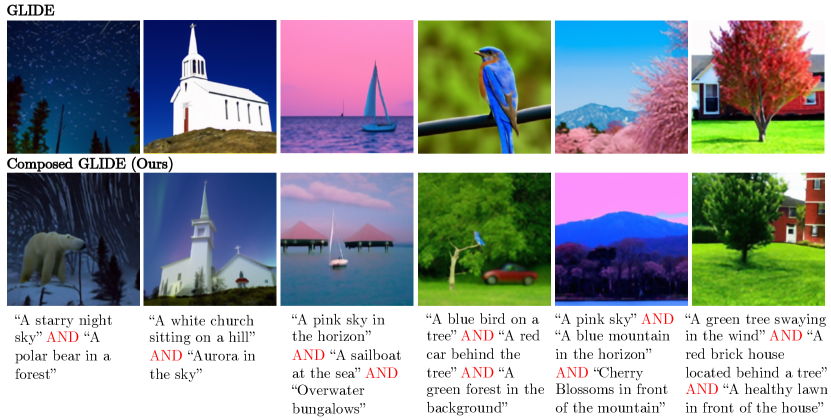
Our approach can effectively compose natural language descriptions. We first show the image generation results of the pre-trained diffusion model, GLIDE [33], in Figure 3. We develop Composed GLIDE, a version of GLIDE that utilizes our compositional operators to combine textual descriptions, without further training. We compare this model to the original GLIDE model.
In Figure 3, GLIDE takes a single long sentence as input, for example, “A pink sky in the horizon, a sailboat at the sea, and overwater bungalows”. In contrast, Composed GLIDE composes several short sentences using the concept conjunction operator, e.g. “A pink sky in the horizon” AND “A sailboat at the sea” AND “Overwater bungalows”. While both GLIDE and Composed GLIDE can generate reasonable images containing objects described in the text prompt, our approach with the compositional operators can more accurately capture text details, such as the presence of “a polar bear” in the first example and the “overwater bungalows” in the third example.
| Models | 1 Component | 2 Components | 3 Components | |||
|---|---|---|---|---|---|---|
| Acc (%) | FID | Acc (%) | FID | Acc (%) | FID | |
| StyleGAN2-ADA [21] | 37.28 | 57.41 | - | - | - | - |
| StyleGAN2 [23] | 1.04 | 51.37 | 0.04 | 23.29 | 0.00 | 19.01 |
| LACE [36] | 0.70 | 50.92 | 0.00 | 22.83 | 0.00 | 19.62 |
| GLIDE [33] | 0.86 | 61.68 | 0.06 | 38.26 | 0.00 | 37.18 |
| EBM [7] | 70.54 | 78.63 | 28.22 | 65.45 | 7.34 | 58.33 |
| Ours | 86.42 | 29.29 | 59.20 | 15.94 | 31.36 | 10.51 |
6.3 Composing Objects
Given a set of 2D object positions, we aim to generate images containing objects at those positions.
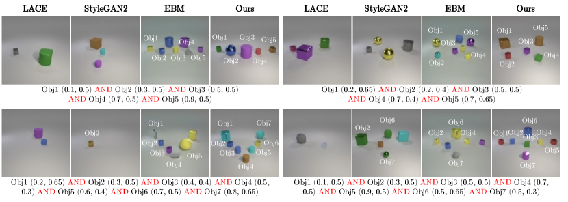
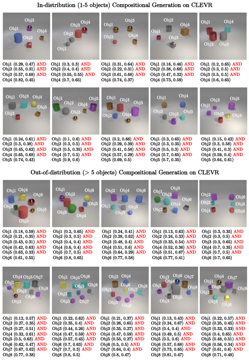
Qualitative results. We compare the proposed method and baselines on composing objects in Figure 4. We only show the concept conjunction here because the object positions are not binary values, and thus negation of object positions is not interpretable. Given a set of object position labels, we compose them to generate images. Our model can generate images of objects at certain locations, while the baseline methods either miss objects or generate incorrect objects.
Quantitative results. As shown in Table 1, our method outperforms baselines by a large margin. The binary classification accuracy of our method is higher than the best baseline, EBM, in the 1 component test setting and is higher than EBM in the more challenging 3 Components setting. Our method is more effective in zero-shot compositional generalization. In addition, our method can generate images with lower FID scores, indicating the generated images are more similar to real images.
| Models | 1 Component | 2 Components | 3 Components | |||
|---|---|---|---|---|---|---|
| Acc (%) | FID | Acc (%) | FID | Acc (%) | FID | |
| StyleGAN2-ADA [21] | 67.71 | 20.55 | - | - | - | - |
| StyleGAN2 [23] | 20.18 | 22.29 | 1.66 | 30.58 | 0.16 | 31.30 |
| LACE [36] | 1.10 | 40.54 | 0.10 | 40.61 | 0.04 | 40.60 |
| GLIDE [33] | 46.20 | 17.61 | 8.86 | 28.56 | 1.36 | 40.02 |
| EBM [28] | 78.14 | 44.41 | 24.16 | 55.89 | 4.26 | 58.66 |
| Ours | 60.40 | 29.06 | 21.84 | 29.82 | 2.80 | 26.11 |
6.4 Composing Object Relations
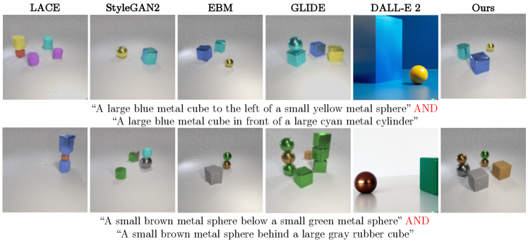
Qualitative results. We further compare the proposed approach and baselines on composing object relational descriptions in Figure 5. Our model is trained to generate images conditioned on a single object relation, but it can compose multiple object relations during inference without additional training. Both LACE and StyleGAN2 fail to capture object relations in the input sentences, but EBM and our method can correctly compose multiple object relations. Our method generates higher-quality images compared with EBM, e.g. the object boundaries are sharper in our results than EBM. Surprisingly, DALL-E 2 and GLIDE can generate high-quality images, but they fail to understand object relations.
Quantitative results. Similarly to experiments in section 6.3, we evaluate the proposed method and baselines on three test settings in Table 2. We train a binary classifier to evaluate whether an image contains objects that satisfy the input relational descriptions. For binary classification accuracy, our method outperforms StyleGAN2, LACE, and GLIDE on all three test settings. EBMs perform well on composing relational descriptions, but their FID scores are much worse than other methods, i.e. their generated images are not realistic. StyleGAN2-ADA can obtain better accuracy and FID than our approach, but it cannot compose multiple concepts.
6.5 Results analysis
We show our composed results on image generation and the results generated conditioned on each individual sentence description in Figure 6. We provide four successfully composed examples, where the generated images contain all the concepts mentioned in the input sentences.
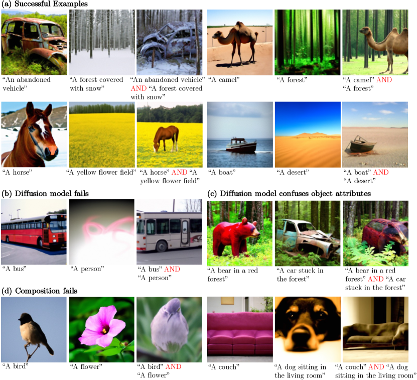
Failure cases. We observed three main failure cases of the proposed method. The first one is that the pre-trained diffusion models do not understand certain concepts, such as “person” in (b). This is because the pre-trained diffusion model, GLIDE [33], is trained to avoid generating human images. The second type of failure is because the diffusion models confuse the objects’ attributes. In (c), the generated image contains “a red bear” while the input is “a bear in a red forest”. The third type of failure is because the composition does not work, e.g. the “bird-shape and flower-color object” and the “dog-fur and sofa-shape object” in (d). Such failures usually happen when the objects are in the center of the images.
7 Conclusion
In this paper, we compose diffusion models for image generation. By interpreting diffusion models as energy-based models, we may explicitly compose them and generate images with significantly more complex combinations that are never seen during training. We propose two compositional operators, concept conjunction and negation, allowing us to compose diffusion models during the inference time without any additional training. The proposed composable diffusion models can generate images conditioned on sentence descriptions, objects, object relations, and human facial attributes, and can generalize to new combinations that are rarely seen in the real world. These results demonstrate the effectiveness of the proposed method for compositional visual generation.
A limitation of our current approach is that while we can compose multiple diffusion models together, they are instances of the same model. We found limited success when composing diffusion models trained on different datasets. In contrast, compositional generation with EBMs [7] can successfully compose multiple separately trained models. Incorporating additional structures into diffusion models from EBMs [10], such as a conservative score field, can be a promising direction towards compositions of separately trained diffusion models.
References
- [1] Austin, J., Johnson, D.D., Ho, J., Tarlow, D., van den Berg, R.: Structured denoising diffusion models in discrete state-spaces. In: Advances in Neural Information Processing Systems (2021)
- [2] Bau, D., Andonian, A., Cui, A., Park, Y., Jahanian, A., Oliva, A., Torralba, A.: Paint by word. arXiv preprint arXiv:2103.10951 (2021)
- [3] Chen, N., Zhang, Y., Zen, H., Weiss, R.J., Norouzi, M., Chan, W.: Wavegrad: Estimating gradients for waveform generation. arXiv preprint arXiv:2009.00713 (2020)
- [4] Chomsky, N.: Aspects of the Theory of Syntax. The MIT Press, Cambridge (1965), http://www.amazon.com/Aspects-Theory-Syntax-Noam-Chomsky/dp/0262530074
- [5] DCGM: Gender, age, and emotions extracted for flickr-faces-hq dataset (ffhq). https://github.com/DCGM/ffhq-features-dataset (2020)
- [6] Dhariwal, P., Nichol, A.: Diffusion models beat gans on image synthesis. Advances in Neural Information Processing Systems 34 (2021)
- [7] Du, Y., Li, S., Mordatch, I.: Compositional visual generation with energy based models. Advances in Neural Information Processing Systems 33, 6637–6647 (2020)
- [8] Du, Y., Li, S., Sharma, Y., Tenenbaum, J., Mordatch, I.: Unsupervised learning of compositional energy concepts. Advances in Neural Information Processing Systems 34 (2021)
- [9] Du, Y., Li, S., Tenenbaum, J., Mordatch, I.: Improved contrastive divergence training of energy based models. arXiv preprint arXiv:2012.01316 (2020)
- [10] Du, Y., Mordatch, I.: Implicit generation and generalization in energy-based models. arXiv preprint arXiv:1903.08689 (2019)
- [11] Gao, R., Song, Y., Poole, B., Wu, Y.N., Kingma, D.P.: Learning energy-based models by diffusion recovery likelihood. In: International Conference on Learning Representations (2021), https://openreview.net/forum?id=v_1Soh8QUNc
- [12] Grathwohl, W., Wang, K.C., Jacobsen, J.H., Duvenaud, D., Zemel, R.: Learning the stein discrepancy for training and evaluating energy-based models without sampling. In: International Conference on Machine Learning (2020)
- [13] Gu, S., Chen, D., Bao, J., Wen, F., Zhang, B., Chen, D., Yuan, L., Guo, B.: Vector quantized diffusion model for text-to-image synthesis. In: Proceedings of the IEEE/CVF Conference on Computer Vision and Pattern Recognition. pp. 10696–10706 (2022)
- [14] Hinton, G.E.: Training products of experts by minimizing contrastive divergence. Neural computation 14(8), 1771–1800 (2002)
- [15] Ho, J., Jain, A., Abbeel, P.: Denoising diffusion probabilistic models. Advances in Neural Information Processing Systems 33, 6840–6851 (2020)
- [16] Ho, J., Salimans, T.: Classifier-free diffusion guidance. In: NeurIPS 2021 Workshop on Deep Generative Models and Downstream Applications (2021)
- [17] Huang, G., Liu, Z., Van Der Maaten, L., Weinberger, K.Q.: Densely connected convolutional networks. In: Proceedings of the IEEE conference on computer vision and pattern recognition. pp. 4700–4708 (2017)
- [18] Janner, M., Du, Y., Tenenbaum, J., Levine, S.: Planning with diffusion for flexible behavior synthesis. In: International Conference on Machine Learning (2022)
- [19] Johnson, J., Hariharan, B., Van Der Maaten, L., Fei-Fei, L., Lawrence Zitnick, C., Girshick, R.: Clevr: A diagnostic dataset for compositional language and elementary visual reasoning. In: Proceedings of the IEEE conference on computer vision and pattern recognition. pp. 2901–2910 (2017)
- [20] Karras, T., Aila, T., Laine, S., Lehtinen, J.: Progressive growing of gans for improved quality, stability, and variation. arXiv preprint arXiv:1710.10196 (2017)
- [21] Karras, T., Aittala, M., Hellsten, J., Laine, S., Lehtinen, J., Aila, T.: Training generative adversarial networks with limited data. Advances in Neural Information Processing Systems 33, 12104–12114 (2020)
- [22] Karras, T., Laine, S., Aila, T.: A style-based generator architecture for generative adversarial networks. In: Proceedings of the IEEE/CVF conference on computer vision and pattern recognition. pp. 4401–4410 (2019)
- [23] Karras, T., Laine, S., Aittala, M., Hellsten, J., Lehtinen, J., Aila, T.: Analyzing and improving the image quality of stylegan. In: Proceedings of the IEEE/CVF conference on computer vision and pattern recognition. pp. 8110–8119 (2020)
- [24] Kim, G., Kwon, T., Ye, J.C.: Diffusionclip: Text-guided diffusion models for robust image manipulation. In: Proceedings of the IEEE/CVF Conference on Computer Vision and Pattern Recognition (CVPR). pp. 2426–2435 (June 2022)
- [25] Kingma, D.P., Ba, J.: Adam: A method for stochastic optimization. arXiv preprint arXiv:1412.6980 (2014)
- [26] Lake, B.M., Salakhutdinov, R., Tenenbaum, J.B.: Human-level concept learning through probabilistic program induction. Science 350(6266), 1332–1338 (2015). https://doi.org/10.1126/science.aab3050, https://www.science.org/doi/abs/10.1126/science.aab3050
- [27] LeCun, Y., Chopra, S., Hadsell, R., Ranzato, M., Huang, F.: A tutorial on energy-based learning. Predicting structured data 1(0) (2006)
- [28] Liu, N., Li, S., Du, Y., Tenenbaum, J., Torralba, A.: Learning to compose visual relations. Advances in Neural Information Processing Systems 34 (2021)
- [29] Lorensen, W.E., Cline, H.E.: Marching cubes: A high resolution 3d surface construction algorithm. ACM siggraph computer graphics 21(4), 163–169 (1987)
- [30] Loshchilov, I., Hutter, F.: Decoupled weight decay regularization. arXiv preprint arXiv:1711.05101 (2017)
- [31] Marcus, G., Davis, E., Aaronson, S.: A very preliminary analysis of dall-e 2. arXiv preprint arXiv:2204.13807 (2022)
- [32] Meng, C., He, Y., Song, Y., Song, J., Wu, J., Zhu, J.Y., Ermon, S.: Sdedit: Guided image synthesis and editing with stochastic differential equations. In: International Conference on Learning Representations (2021)
- [33] Nichol, A., Dhariwal, P., Ramesh, A., Shyam, P., Mishkin, P., McGrew, B., Sutskever, I., Chen, M.: Glide: Towards photorealistic image generation and editing with text-guided diffusion models. arXiv preprint arXiv:2112.10741 (2021)
- [34] Nichol, A., Jun, H., Dhariwal, P., Mishkin, P., Chen, M.: Point-e: A system for generating 3d point clouds from complex prompts. arXiv preprint arXiv:2212.08751 (2022)
- [35] Nichol, A.Q., Dhariwal, P.: Improved denoising diffusion probabilistic models. In: International Conference on Machine Learning. pp. 8162–8171. PMLR (2021)
- [36] Nie, W., Vahdat, A., Anandkumar, A.: Controllable and compositional generation with latent-space energy-based models. Advances in Neural Information Processing Systems 34 (2021)
- [37] Nijkamp, E., Hill, M., Han, T., Zhu, S.C., Wu, Y.N.: On the anatomy of mcmc-based maximum likelihood learning of energy-based models. arXiv preprint arXiv:1903.12370 (2019)
- [38] Parmar, G., Zhang, R., Zhu, J.Y.: On aliased resizing and surprising subtleties in gan evaluation. In: CVPR (2022)
- [39] Ramesh, A., Dhariwal, P., Nichol, A., Chu, C., Chen, M.: Hierarchical text-conditional image generation with clip latents. arXiv preprint arXiv:2204.06125 (2022)
- [40] Ramesh, A., Pavlov, M., Goh, G., Gray, S., Voss, C., Radford, A., Chen, M., Sutskever, I.: Zero-shot text-to-image generation. In: International Conference on Machine Learning. pp. 8821–8831. PMLR (2021)
- [41] Rombach, R., Blattmann, A., Lorenz, D., Esser, P., Ommer, B.: High-resolution image synthesis with latent diffusion models. In: Proceedings of the IEEE/CVF Conference on Computer Vision and Pattern Recognition. pp. 10684–10695 (2022)
- [42] Rombach, R., Blattmann, A., Lorenz, D., Esser, P., Ommer, B.: High-resolution image synthesis with latent diffusion models (2021)
- [43] Saharia, C., Chan, W., Chang, H., Lee, C.A., Ho, J., Salimans, T., Fleet, D.J., Norouzi, M.: Palette: Image-to-image diffusion models. arXiv preprint arXiv:2111.05826 (2021)
- [44] Salimans, T., Ho, J.: Should ebms model the energy or the score? In: Energy Based Models Workshop-ICLR 2021 (2021)
- [45] Shoshan, A., Bhonker, N., Kviatkovsky, I., Medioni, G.: Gan-control: Explicitly controllable gans. In: Proceedings of the IEEE/CVF International Conference on Computer Vision. pp. 14083–14093 (2021)
- [46] Sohl-Dickstein, J., Weiss, E., Maheswaranathan, N., Ganguli, S.: Deep unsupervised learning using nonequilibrium thermodynamics. In: International Conference on Machine Learning. pp. 2256–2265. PMLR (2015)
- [47] Song, J., Meng, C., Ermon, S.: Denoising diffusion implicit models. In: International Conference on Learning Representations (2021)
- [48] Song, Y., Sohl-Dickstein, J., Kingma, D.P., Kumar, A., Ermon, S., Poole, B.: Score-based generative modeling through stochastic differential equations. arXiv preprint arXiv:2011.13456 (2020)
- [49] Swimmer963: What dall-e 2 can and cannot do (May 2022), https://www.lesswrong.com/posts/uKp6tBFStnsvrot5t/what-dall-e-2-can-and-cannot-do
- [50] Szegedy, C., Vanhoucke, V., Ioffe, S., Shlens, J., Wojna, Z.: Rethinking the inception architecture for computer vision. In: Proceedings of the IEEE conference on computer vision and pattern recognition. pp. 2818–2826 (2016)
- [51] Vincent, P.: A connection between score matching and denoising autoencoders. Neural computation 23(7), 1661–1674 (2011)
- [52] Xiao, T., Hong, J., Ma, J.: Elegant: Exchanging latent encodings with gan for transferring multiple face attributes. In: Proceedings of the European conference on computer vision (ECCV). pp. 168–184 (2018)
- [53] Xu, T., Zhang, P., Huang, Q., Zhang, H., Gan, Z., Huang, X., He, X.: Attngan: Fine-grained text to image generation with attentional generative adversarial networks. In: Proceedings of the IEEE conference on computer vision and pattern recognition. pp. 1316–1324 (2018)
- [54] Zhang, H., Xu, T., Li, H., Zhang, S., Wang, X., Huang, X., Metaxas, D.N.: Stackgan: Text to photo-realistic image synthesis with stacked generative adversarial networks. In: Proceedings of the IEEE international conference on computer vision. pp. 5907–5915 (2017)
- [55] Zhou, L., Du, Y., Wu, J.: 3D shape generation and completion through point-voxel diffusion. In: International Conference on Computer Vision (2021)
- [56] Zhu, J., Shen, Y., Zhao, D., Zhou, B.: In-domain gan inversion for real image editing. In: European conference on computer vision. pp. 592–608. Springer (2020)
Appendix
In this appendix, we first demonstrate additional results in appendix 0.A. We then show the details of training classifiers in appendix 0.B. In appendix 0.C and appendix 0.D, we show more details of our approach and baselines, respectively. Next, we provide the implementation details in appendix 0.E. Finally, we provide derivations of both the conjunction and negation operators in appendix 0.F.
Appendix 0.A Additional Results
In this section, we first show the results of composing language descriptions to generate 3D meshes in section 0.A.1. We then show the results of composing human facial attributes in section 0.A.2. Finally, we show more qualitative results in section 0.A.3.
0.A.1 Composing Language Descriptions for 3D Asset Generation
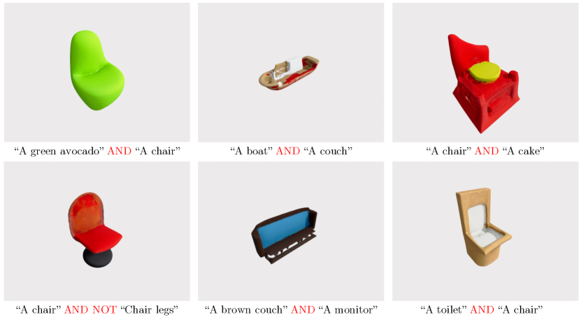
Qualitative results. We demonstrate the proposed method of composing language descriptions for point cloud generation, which can be further used to generate 3D meshes. We first use Point-E [34], the pre-trained 3D point cloud generation model, to generate the point clouds of an object based on the text description. We then convert the 3D point clouds into 3D meshes using marching cubes [29]. The results are shown in Figure 7.
0.A.2 Composing Human Facial Attributes
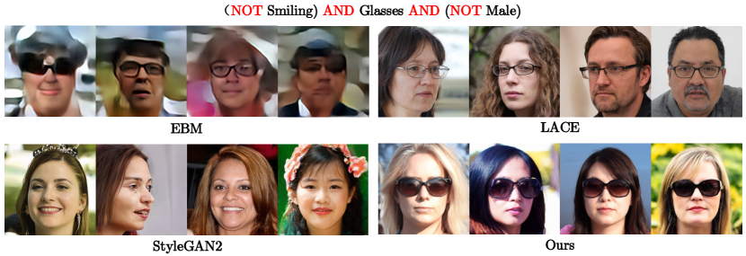
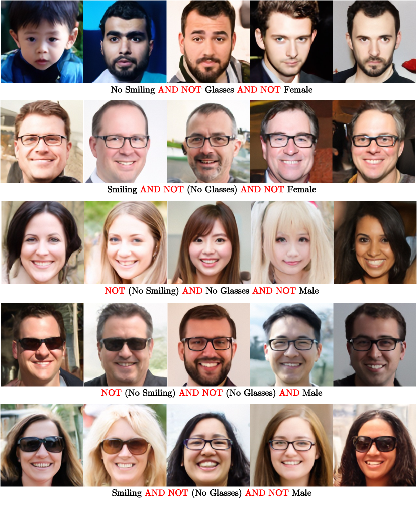
Qualitative results. We compare the proposed method and baselines on composing facial attributes in Figure 8. We find that LACE and StyleGAN2 can generate high-fidelity images, but the generated images do not match the given labels. For example, StyleGAN2 generates humans without wearing glasses when the input label contains Glasses, while LACE generates males sometimes when the input is Not Male. The image quality of EBM is much worse than other methods. In contrast, our method can generate high-fidelity images, containing all the attributes in the input label.
Quantitative results. The results of our method and baselines on three test settings are shown in Table 3. Our method is comparable with the best baseline on each evaluation metric.
0.A.3 More Qualitative Results
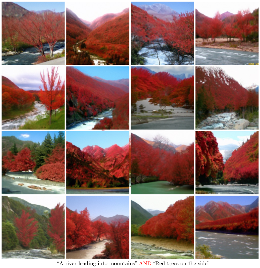
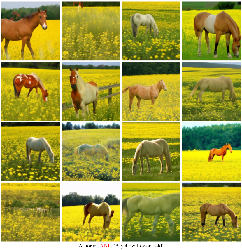
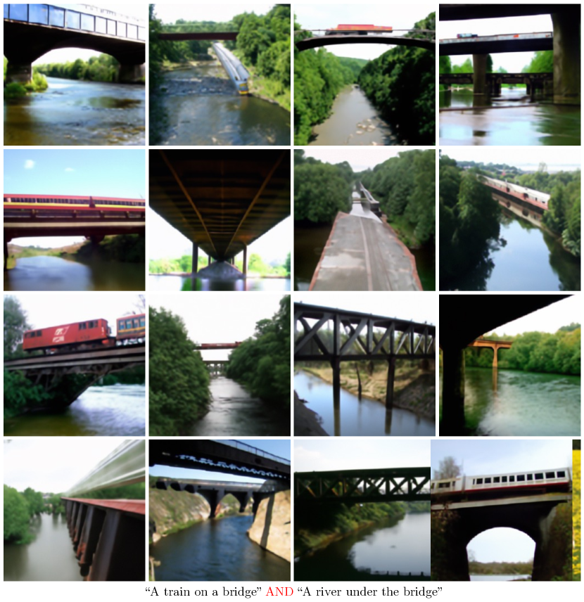
We provide more qualitative results of the proposed method on composing concepts using the conjunction operator. Figure 10, Figure 11, Figure 12, and Figure 13 show more results of composing language descriptions. Figure 14 shows additional results on composing objects on the CLEVR dataset. Our approach can reliably generate images conditioned on multiple concepts, even for combinations that are outside the training distribution.
We further show the results of composing facial attributes on the FFHQ dataset in Figure 15. Our model is trained to generate images conditioned on a single human facial attribute, but it can compose multiple attributes during inference without further training by using the conjunction and negation compositional operators. As shown in the fifth row of Figure 15, our model can compose Not Male and Glasses and generate images with females wearing glasses. The proposed compositional operators allow our model to compose facial attributes recursively.
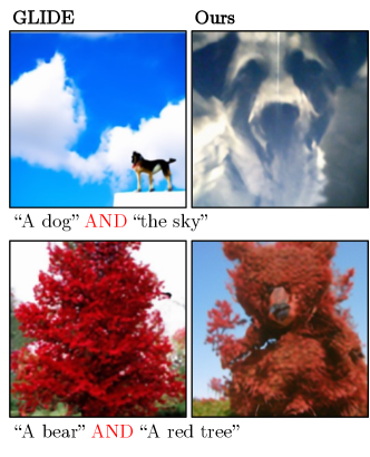
Interesting cases. As shown in Figure 9, we find that our method, which combines multiple textual descriptions, can generate different styles of images compared to GLIDE, which directly encodes the descriptions as a single long sentence. Taking “a dog” and “the sky” as inputs, our method generates a dog-shaped cloud, whereas GLIDE generates a dog under the sky using the prompt “a dog and the sky”.
| Models | 1 Component | 2 Components | 3 Components | |||
|---|---|---|---|---|---|---|
| Acc () | FID | Acc () | FID | Acc () | FID | |
| StyleGAN2-ADA [21] | 91.06 | 10.75 | - | - | - | - |
| StyleGAN2 [23] | 58.90 | 18.04 | 30.68 | 18.06 | 16.96 | 18.06 |
| LACE [36] | 97.60 | 28.21 | 95.66 | 36.23 | 80.88 | 34.64 |
| GLIDE [33] | 98.66 | 20.30 | 48.68 | 22.69 | 27.24 | 21.98 |
| EBM [7] | 98.74 | 89.95 | 93.10 | 99.64 | 30.01 | 335.70 |
| Ours | 99.26 | 18.72 | 92.68 | 17.22 | 68.86 | 16.95 |
Appendix 0.B Details of Binary Classifiers
We provide more details of the binary classifiers in this section.
CLEVR. The CLEVR dataset consists of 30,000 image-label pairs. We split the dataset into training and validation subsets. There are data pairs used for training and data pairs used for validation. We train a binary classifier to evaluate whether there is an object appearing at a particular position of an image. The classifier achieves an accuracy of on the validation set, which is used to evaluate the quality of generated images.
Relational CLEVR. The Relational CLEVR [28] dataset contains images at resolution. We split the dataset into training data and validation data. Then we train a binary classifier to evaluate whether an image contains an object relational description. The trained classifier achieves an accuracy of on the validation set.
FFHQ. We use image-label pairs from CelebA-HQ [20] to train a classifier to evaluate the generated images. We split the dataset into the training ( data pairs) and validation ( data pairs) subsets. We select three attributes (i.e. smiling, glasses, and gender) to evaluate the compositional ability of our approach and baselines. We thus train three binary classifiers to evaluate the smiling, glasses, and gender concepts, respectively. Our classifiers achieve , and accuracy on the validation sets of smiling, glasses, and gender, respectively.
Appendix 0.C Details of Our Approach
Training. Our approach is implemented based on the code from [35, 33]. Ho et al. [16] introduce a technique to train the conditional and unconditional diffusion models at the same time by masking some labels as nulls. We use the same approach to train diffusion models. For each data point, its label has a chance of being replaced by a null label which is used to estimate the unconditional score.
Inference. To generate FFHQ images, we first generate images at resolution and then upsample the images to using a sampler provided by [33]. For CLEVR images, we generate images at resolution directly.
Label Encoding. On the FFHQ dataset, we use three human facial attributes, i.e. smile, glasses and gender. For the smile and glasses attributes, label indicates an image containing the attribute; otherwise, the label is . For the gender attribute, label indicates “male”, while label represents “female”. We use the embedding layer to encode the attribute labels. The first six dimensions represent the attribute labels and the last dimension indicates the null class. The labels are encoded as a -dimension feature vector, which is then fused with the time embedding to estimate the score .
On the CLEVR dataset, we encode the coordinates using a linear layer , where is the dimension of the output feature. The coordinate embedding is then fused with the time embedding to estimate the score .
Appendix 0.D Details of Baselines
StyleGAN2-ADA. On each dataset, we train a conditional StyleGAN2-ADA model using the “stylegan” configuration provided by [21] without using augmentations.
StyleGAN2. We use the pre-trained StyleGAN2 model [23] to evaluate its performance on facial image generation. As there is no pre-trained model for object generation, we use the same code to train a model on the CLEVR dataset for image generation conditioned on object positions. We use the “config-f” setting provided by [23]. To enable image generation conditioned on multiple concepts, we train a binary classifier on each task. During inference, we optimize the latent code z by decreasing the binary classification loss of the generated image and the given label. We use the resultant latent code to generate images.
LACE. LACE [36] trains classifiers for image generation using the generated images from StyleGAN2 and labels provided by the neural network. For the CLEVR dataset, we first generate images using the same StyleGAN2 model that was trained on CLEVR in Section 0.D. Then we modify the code to train a position annotator using a DenseNet [17] model provided by LACE to label the object positions of generated images. Lastly, we train a classifier conditioned on object coordinates using the code provided by [36]. For FFHQ, we use the off-the-shelf pre-trained model from [36] for comparison.
GLIDE. We use the small GLIDE model released by [33] in our experiments. We develop Composed GLIDE (Ours), a version of GLIDE that utilizes our compositional operators to combine textual descriptions, without further training. We compare it to the original GLIDE, which directly encodes the descriptions as a single long sentence. [33] also releases an upsampler model to upsample the generated images from a resolution of to a resolution of . We use the upsampler model for both the GLIDE and Composed GLIDE (Ours).
Appendix 0.E Implementation Details
Each model is trained on a single Tesla V100 32GB GPU.
StyleGAN2-ADA. Each conditional StyleGAN2-ADA model is trained for two days. We use the Adam optimizer [25] with and to train the models.
StyleGAN2. We train a StyleGAN2 model for two days on both CLEVR and Relational CLEVR datasets. We use the Adam optimizer [25] with and to train the StyleGAN2 models. It takes 2 hours to train a binary classifier. The classifiers are trained using the Adam optimizer with and . For the FFHQ dataset, We use the pre-trained model provided by [23].
LACE. LACE uses the pre-trained model provided by [23] on the FFHQ dataset. For both CLEVR and Relational CLEVR datasets, we directly reuse the trained StyleGAN2 model as described in Section 0.E. It takes less than minutes to train the classifier on each dataset.
EBMs. In our experiments, we use the same setting to train models on different datasets. We use the Adam optimizer [25] with a learning rate of . For MCMC sampling, we use a step size of 300 and 80 iterations. Similarly, the model is trained for two days on each dataset.
Ours. To train diffusion models on CLEVR and FFHQ, we use diffusion steps, and the cosine noise schedule. We use the AdamW optimizer [30] with and . We train the diffusion models on CLEVR for seven days ( iterations) and FFHQ for two days ( iterations).
Appendix 0.F Derivation
0.F.1 Conjunction Operator (AND)
Given a set of independent concepts , the joint probability distribution can be factorized as follows:
| (16) |
We can rewrite above expression using :
| (17) |
Then we take a gradient of logarithm on both sides w.r.t :
| (18) |
Finally, we may obtain a modified score prediction from the above expression , where controls the temperature of each implicit classifier:
| (19) |
In the setting where only one concept is conditioned for sampling, the above equation will reduce to classifier-free guidance [16]:
| (20) |
where the temperature scaling .
0.F.2 Negation Operator (NOT)
Given two independent concepts , the joint probability distribution where we negate the concept can be similarly written as:
| (21) |
Then we take a gradient of logarithm on both sides w.r.t as follows:
| (22) |
Finally, we may obtain a modified score prediction from the above, where is a tunable coefficient that determines the weight of the negation:
| (23) |