Optimal Design of Electric Machine with Efficient Handling of Constraints and Surrogate Assistance

Abstract

Electric machine design optimization is a computationally expensive multi-objective optimization problem. While the objectives require time-consuming finite element analysis, optimization constraints can often be based on mathematical expressions, such as geometric constraints. This article investigates this optimization problem of mixed computationally expensive nature by proposing an optimization method incorporated into a popularly-used evolutionary multi-objective optimization algorithm – NSGA-II. The proposed method exploits the inexpensiveness of geometric constraints to generate feasible designs by using a custom repair operator. The proposed method also addresses the time-consuming objective functions by incorporating surrogate models for predicting machine performance. The article successfully establishes the superiority of the proposed method over the conventional optimization approach. This study clearly demonstrates how a complex engineering design can be optimized for multiple objectives and constraints requiring heterogeneous evaluation times and optimal solutions can be analyzed to select a single preferred solution and importantly harnessed to reveal vital design features common to optimal solutions as design principles.

1 Introduction

Electric machines are essential components within a multitude of industries today and their range of application varies from refrigeration and industrial pumps to power generation and automobiles. Consequently, design optimization of electric machines is a complex multi-objective optimization problem (MOOP) often involving combined analysis of electromagnetic, thermal, and structural performance. Analysis of electric machines is a time-consuming process and therefore, a lot of effort has been focused on improving the optimization tools and efficiency in the past two decades.

From investigating pattern search and sequential unconstrained minimization techniques (Ramarathnam, Desai, and Rao 1973; Singh et al. 1983) to employing evolutionary algorithms (EAs) for optimization of electric machines (Bianchi and Bolognani 1998), electric machine community has continually adopted the improvements in optimization algorithms. As EAs perform better than classical direct search methods in finding global optimum their utilization in electric machine optimization has gained further popularity (Mirzaeian et al. 2002; Sudhoff et al. 2005; Žarko, Ban, and Lipo 2005; Duan, Harley, and Habetler 2009; Duan and Ionel 2013; Zhang et al. 2013). It is also worth mentioning that electric machines require finite element analysis (FEA) for performance evaluation with high accuracy. Naturally, application of EAs in combination with FEA can also be found in literature (Pellegrino and Cupertino 2010a; Pellegrino and Cupertino 2010b). Although combination of EAs with FEA ensures finding optimal solutions with high quality, it also increases the overall computational cost of optimization. In this regard, exploration of computationally inexpensive methods, such as surrogate models, to predict performance of electric machines has led to reduction in overall computational effort (Jolly, Jabbar, and Qinghua 2005; Ionel and Popescu 2009; Sizov, Ionel, and Demerdash 2012; Taran, Ionel, and Dorrell 2018; Song et al. 2018).

A comprehensive literature review shows that while efforts have been made to improve the optimization tools and efficiency, constraints handling, specifically inexpensive constraints (such as geometric), in electrical machine optimization deserves more attention. More commonly, the geometric feasibility of a candidate solution during optimization relies on random sampling. For instance, in each optimization cycle (generation), geometrically infeasible solutions are discarded, and a random initialization may be repeated until the desired number of feasible solutions has been found (Stipetic, Miebach, and Zarko 2015). However, this random sampling may be inefficient when the number of geometric variables and constraints increases. Khoshoo et al. (2021) presented a preliminary study showing that the information from inexpensive constraints can be used to repair geometrically infeasible solutions and improve the Pareto-optimal front. However, this preliminary study did not address the computational expense of the objective functions vital for electric machine design optimization. Thus, this article extends the algorithm repairing infeasible designs by incorporating surrogate models to address the time-consuming objective functions. The main contributions of this work are as follows.

• Proposal of a repair operator which improves the quality of Pareto-optimal front by ensuring geometrically feasible solutions in each optimization cycle by exploiting the inexpensiveness of geometric constraints, while also respecting the manufacturing accuracy limitations.

• Performance validation of the proposed repair operator in combination with surrogates to predict the computationally expensive objective functions and their impact on the convergence of the optimization algorithm.

• Insights gained from Pareto-optimal electric machine designs and recommendations for selecting preferred solutions based on two different approaches: (1) a domain specific a posteriori multi-criteria decision-making (MCDM) method involving machine expertise, and (2) trade-off analysis of the Pareto-optimal set.

The rest of this article is structured as follows. Section 2 discusses related work and reviews optimization methods proposed to optimize electric machine design. Section 3 discusses the formulation of the optimization problem used in this article. Section 4 presents the proposed optimization method exploiting the computationally inexpensive constraints using a repair operator and addressing the computationally expensive objectives by incorporating surrogate models. The impact of the algorithm’s components on the convergence of the algorithm, along with a detailed discussion about Pareto-optimal solutions and selection of preferred electric machine designs, is discussed in Section 5. Finally, conclusions are presented in Section 6.

2 Related Work

Advancements in optimization algorithms and objective function evaluation tools have facilitated the design optimization of electric machines. Ramarathnam, Desai, and Rao (1973) presented an early case study involving an induction machine’s design by solving a single objective optimization problem. The authors compared the performance of a direct, indirect, and random search method in conjunction with the sequential unconstrained minimization technique. Results showed that a direct search method performs better for complicated multi-variable functions commonly occurring in electric machines. However, optimization methods considered in the study suffered from getting stuck in local optima and required several restarts to reach the global optimum.

Metaheuristics, particularly Genetic Algorithms (GAs), are widely used and known for their global search behavior. Bianchi and Bolognani (1998) used a GA to optimize the design of a surface-mounted permanent magnet (SPM) machine. Results from two independent single objective optimization problems indicated that an evolutionary method outperforms the direct search method when comparing the convergence to the global optimum.

Since the design of an electric machine typically includes comparing the performance of multiple metrics, multi-objective optimization using EAs is predominantly employed nowadays. For instance, Pellegrino and Cupertino (2010b) employed an EA combined with FEA to solve a three-objective optimization problem. The authors compared two partial optimization strategies with a comprehensive three-objective optimization method. Results showed that domain knowledge could be utilized to modify the optimization problem creatively to reduce the computation time without significantly affecting the quality of results.

Several other strategies have been proposed for the reduction of optimization run-time. For example, Pellegrino, Cupertino, and Gerada (2015) proposed a local refinement strategy to improve a Pareto-optimal design further after the optimization terminated. After selecting a design in the region of interest, a local optimization method was employed in the design’s vicinity. Results showed that an a posteriori local search, even with fewer function evaluations, produced similar results to those by an approach solely relying on global optimization. Similarly, Degano et al. (2016) split the optimization procedure into two phases, where authors optimized torque density and losses in the first stage and the quality of torque profile in the second stage. Although average torque and ripple are conflicting objectives, the optimal solutions after the second stage showed improved torque ripple without compromising the average torque.

Another research direction to address computationally expensive functions during optimization is the usage of surrogate models. For example, Jolly, Jabbar, and Qinghua (2005) used second-order response surface models (RSM) to predict d-axis and q-axis inductances and magnet flux linkage of an IPM machine to optimize the magnet shape and placement in the machine’s rotor. Similarly, Taran, Ionel, and Dorrell (2018) presented a two-level surrogate-assisted optimization approach using DE to find optimal designs for Axial Flux PM (AFPM) machines by minimizing active material mass and total losses at rated operation. Results showed that the surrogate-assisted algorithm outperforms the conventional multi-objective DE in terms of computation time. It is worth mentioning that usage of surrogates introduces a trade-off between computation time and solution accuracy.

It is clear from the review of past studies that constraint handling, especially when the constraints are inexpensive, in an electric machine design optimization problem requires more attention. This article addresses this gap in research by first introducing an electric machine design problem of mixed computationally expensive nature and then proposes an optimization method that exploits the inexpensiveness of constraints.

3 Electric Machine Design And Optimization Problem Formulation

In addition to selection of objective functions, design variables, variable ranges, and constraints like every other MOOP, an electric machine design optimization problem also requires selection of a machine template which is primarily application dependant. In this article, a 3-phase, 48-slot/8-pole IPM machine with a single layer of V-shaped magnet, used in 2010 Toyota Prius, is chosen for analysis. 2D model of the machine is shown in Figure 1(a) (Altair 2019). In this article, two of the most common machine performance measures, average torque and torque pulsations are chosen as the objective functions which are calculated using FEA. To reduce the simulation run time, periodicity in 2D model is taken advantage of and only $1/8^{th}$ of the model is simulated as shown in Figure 1(b). Both objective functions are conflicting and optimization’s goal is to maximize average torque while minimizing torque pulsations, where the definition of pulsations is highlighted in Figure 3.

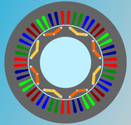
(a) 2d model of machine.

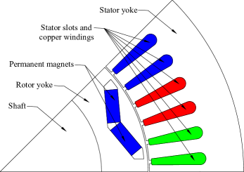
(b) Reduced model used in FEA.

Figure 1: IPM machine used for optimization

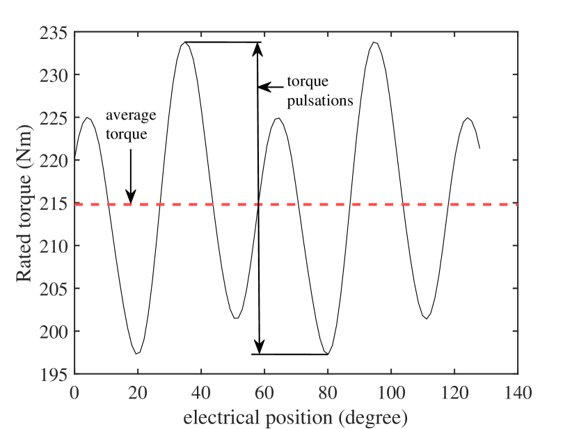
Figure 2: Torque profile of reference mahine at rated operation.

Figure 3: Geometric variables used for optimization.

After the selection of objective functions, a sensitivity analysis study has provided the ten most significant geometric variables, as shown in Figure 3. Variable ranges are defined based on the machine designer’s experience with a $\pm$20% variation from the reference design. Additionally, manufacturing accuracy limitations are applied to all variables by limiting them to have only two decimal places. Details of lower ($x^{(L)}$) and upper ($x^{(U)}$) bounds along with reference ($x^{(ref)}$) values of the ten variables are given in Table 3. Ten geometric constraints ensure the geometric feasibility of candidate designs. All optimization studies are performed for the rated operating point, with the rotational speed of the rotor and the excitation angle kept constant to those of the reference design. Details on the formulation of geometric constraints and the selection of an operating point for optimization are provided in the supplementary document.

Values of geometric variables used for optimization. $x_{i}$ Variable Unit $x^{(\text{ref})}$ $x^{(L)}$ $x^{(U)}$ $x_{1}$ Height of rotor pole cap mm 9.56 7.65 11.47 $x_{2}$ Magnet thickness mm 7.16 5.73 8.59 $x_{3}$ Magnet width mm 17.88 14.30 21.46 $x_{4}$ Angle between magnets degree 145.35 116.28 174.42 $x_{5}$ Bridge height mm 1.99 1.59 2.39 $x_{6}$ Q-axis width mm 13.9 11.12 16.68 $x_{7}$ Slot height mm 30.9 24.72 37.08 $x_{8}$ Slot width mm 6.69 5.35 8.03 $x_{9}$ Height of slot opening mm 1.22 0.98 1.46 $x_{10}$ Width of slot opening mm 1.88 1.50 2.26

Based on the above discussion of electric machine design, a bi-objective optimization problem with ten variables and ten geometric constraints is formulated in this work. Ultimately, the MOOP is defined as

Maximize $$\quad\texttt{Average\ Torque}(\mbox{${\textbf{x}}$}),$$ (1)

Minimize $$\quad\texttt{Torque\ Pulsation}(\mbox{${\textbf{x}}$}),$$

subject to $$\quad g_{j}(\mbox{${\textbf{x}}$})\leq 0, \forall j\in 1,\ldots,10,{}{}$$

$$\quad x_{i}^{(L)}\leq x_{i}\leq x_{i}^{(U)}, \forall i\in 1,\ldots,10,{}$$

where $$\quad\mbox{${\textbf{x}}$}\in\mathbb{R}^{N},$$

where x represent the design variables to optimize, $g_{j}(\mbox{${\textbf{x}}$})$ are the geometric constraints, and the lower and upper bound of the variables are denoted by $x_{i}^{(L)}$ and $x_{i}^{(U)}$ respectively. As explained previously, due to manufacturing accuracy limitations, all variables are restricted to have only two decimal places. Additionally, while the geometric constraints are inexpensive to evaluate, objective functions require time consuming FEA.

4 Proposed Multi-Objective Optimization Algorithm

Based on the discussion presented in the previous section, it can be concluded that the formulated electric machine optimization problem is of mixed computationally expensive nature with two expensive objective functions and ten inexpensive geometric constraints. In a preliminary study, Khoshoo et al. (2021) showed that the computational inexpensiveness of constraint evaluations could be exploited to convert an infeasible solution to a feasible one through a repair operator. Additionally, the design optimization of electric machines is an expensive problem to solve, and some effort must be made to reduce the computational cost. Therefore, in addition to the repair operator, the proposed optimization method incorporates surrogates for predicting expensive objectives. In this study, the evolutionary multi-objective optimization (EMO) algorithm NSGA-II (Deb et al. 2002) is used as the base optimization algorithm. Implementation of repair operator and surrogates in optimization algorithm is explained below.

4.1 Implementation of Repair Operator

Implementation of repair operator focuses on two goals: (1) converting an infeasible solution to a feasible one and (2) satisfying the manufacturing accuracy limitations. While the first goal is achieved via an embedded optimization procedure, the second goal is accomplished by rounding each variable up or down, using an approach inspired by Hooke-Jeeves pattern moves (Hooke and Jeeves 1961). A detailed explanation of the two phases is included in the supplementary document.

4.2 Surrogate Incorporation in Optimization Cycle

Commonly, surrogates – approximation or interpolation models – are utilized during optimization to improve the convergence behavior. First, one shall distinguish between two different types of evaluations: exact solution evaluations (ESEs) that require to run the computationally expensive evaluation for computing two objectives Average Torque(x) and Torque Pulsation(x); and approximate solution evaluations (ASEs) which is a computationally inexpensive approximation by the surrogates. Where the overall optimization run is limited by $\texttt{ESE}^{\max}$ function evaluation, function calls of ASEs are only considered as algorithmic overhead. In order to improve the convergence of NSGA-II, the surrogates provide ASEs and let the algorithm look several iterations into the future without any evaluation of ESEs. The surrogate models are used to create a set of infill solutions as follows: First, NSGA-II is run for $k$ more iterations (starting from the best solutions found so far), returning the solution set $\mbox{${\textbf{X}}$}^{\texttt{(cand)}}$. The number of solutions in $\mbox{${\textbf{X}}$}^{\texttt{(cand)}}$ corresponds to the population size of the algorithm fixed to $100$ solutions in this study. After eliminating duplicates in $\mbox{${\textbf{X}}$}^{\texttt{(cand)}}$, the number of solutions $N$ desired to run using ESEs needs to be selected. The selection first obtains $N$ clusters by running the k-means algorithm and then uses a roulette wheel selection based on the predicted crowding distances. Note that this will introduce some selection bias towards the boundary points as they have been depicted with an infinite crowding distance. Altogether, this results in $N$ solutions to be evaluated using ESEs in the current optimization cycle.

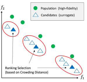
Figure 4: Ranking selection of solutions obtained by optimizing the surrogate-based optimization problem.

Since the electric machine design is formulated with two objectives, two different models are built. Separately fitting a model for each objective corresponds to the M1 method proposed in the surrogate usage taxonomy (Deb et al. 2019). For each objective, the best model type is found by iterating over different model realizations of RBF (Hardy 1971) and Kriging (Krige 1951) varying normalization, regression, and kernel type. Finally, the best model type is chosen based on the validation set’s performance.

4.3 NSGA-II-WR-SA

Algorithm 1 shows how the repair operator and surrogate models are incorporated into the optimization cycle. The algorithm’s parameters are the expensive objective functions F(X) and the inexpensive constraint functions G(X); the maximum number of exact solution evaluations $\texttt{ESE}^{\max}$ serves as an overall termination criterion; the number of the initial design of experiments $N^{\texttt{DOE}}$ describes how many designs are evaluated before optimization starts; the number of solutions $N$ evaluated in each optimization cycle; and the number of surrogate optimization generations $k$, or in other words, how many generations the surrogates are used to look into the future.

Input : Expensive Objective Functions F(X), Inexpensive Constraint Function G(X), Maximum Number of Exact Solution Evaluations $\texttt{ESE}^{\max}$, Number of Initial Design of Experiments $N^{\texttt{DOE}}$, Number of ESEs in Each Optimization Cycle $N$, Number of Surrogate Optimization Generations $k$.

1

2

/* initialize feas. solutions using the inexpensive function $G$ */

3

4$\mbox{${\textbf{X}}$}\leftarrow\texttt{constrained\_sampling}(N^{\texttt{DOE}},\mbox{${\textbf{G}}$})$

5$\mbox{${\textbf{F}}$}\leftarrow\mbox{${\textbf{F}}$}(\mbox{${\textbf{X}}$})$

6

7while $|\mbox{${\textbf{X}}$}|<\texttt{ESE}^{\;\max}$ do

8      

       /* exploitation using the surrogate */

9       $\hat{\mbox{${\textbf{F}}$}}\leftarrow\texttt{fit\_surrogate}(\mbox{${\textbf{X}}$},\mbox{${\textbf{F}}$})$

10      $\left(\mbox{${\textbf{X}}$}^{\texttt{(cand)}},\mbox{${\textbf{F}}$}^{\texttt{(cand)}}\right)\leftarrow\texttt{optimize}(\texttt{'NSGA-II-WR'},\hat{\mbox{${\textbf{F}}$}},\mbox{${\textbf{G}}$},\mbox{${\textbf{X}}$},\mbox{${\textbf{F}}$},k)$

11      $\left(\mbox{${\textbf{X}}$}^{\texttt{(cand)}},\mbox{${\textbf{F}}$}^{\texttt{(cand)}}\right)\leftarrow\texttt{eliminate\_duplicates}(\mbox{${\textbf{X}}$},\mbox{${\textbf{X}}$}^{\texttt{(cand)}},\mbox{${\textbf{F}}$}^{\texttt{(cand)}})$

12      $C\leftarrow\texttt{cluster}(\texttt{'k\_means'},N^{(\texttt{exploit})},\mbox{${\textbf{F}}$}^{\texttt{(cand)}})$

13      $\mbox{${\textbf{X}}$}^{\texttt{(infill)}}\leftarrow\texttt{ranking\_selection}(\mbox{${\textbf{X}}$}^{\texttt{(cand)}},C,\,\texttt{crowding}(\mbox{${\textbf{F}}$}^{\texttt{(cand)}}))$

       /* evaluate and merge to the archive */

14       $\mbox{${\textbf{F}}$}^{\texttt{(infill)}}\leftarrow\mbox{${\textbf{F}}$}(\mbox{${\textbf{X}}$}^{\texttt{(infill)}});$

15      $\mbox{${\textbf{X}}$}\leftarrow\mbox{${\textbf{X}}$}\cup\mbox{${\textbf{X}}$}^{\texttt{(infill)}}$

16      $\mbox{${\textbf{F}}$}\leftarrow\mbox{${\textbf{F}}$}\cup\mbox{${\textbf{F}}$}^{\texttt{(infill)}}$

17      

18 end while

19

Algorithm 1 NSGA-II-WR-SA: A customized version of NSGA-II with a repair of infeasible solutions (WR) and surrogate assistance (SA).

First, the algorithm starts by sampling $N^{\texttt{DOE}}$ solutions in the feasible space using the constrained sampling strategy (Line 1) (Blank and Deb 2021) and evaluates the solution set (Line 1). Then, while the overall evaluation budget $\texttt{ESE}^{\max}$ has not been used yet, surrogates $\hat{\mbox{${\textbf{F}}$}}$ are built for the objectives (Line 1). By applying NSGA-II for $k$ surrogate optimization generations starting from X, using the surrogate models $\hat{\mbox{${\textbf{F}}$}}(\mbox{${\textbf{X}}$})$ and the inexpensive objective functions G(X), a candidate set of solutions $\mbox{${\textbf{X}}$}^{\texttt{(cand)}}$ and $\mbox{${\textbf{F}}$}^{\texttt{(cand)}}$ is retrieved (Line 1). Depending on the surrogate problem, some solutions in $\mbox{${\textbf{X}}$}^{\texttt{(cand)}}$ can be identical to the ones already evaluated in X; thus, duplicate elimination is necessary to ensure these solutions are filtered out (Line 1). Since the size of $\mbox{${\textbf{X}}$}^{\texttt{(cand)}}$ exceeds $N$, a subset solution based on the predicted crowding distances takes place (Line 1 and 1). Finally, the resulting solution set $\mbox{${\textbf{X}}$}^{\texttt{(infill)}}$ of size $N$ is evaluated using ESEs and is appended to the archive of solutions.

5 Results and Discussion

In this section, the performance of the proposed optimization method is investigated and following key questions are answered.

• How does the repair operator help the optimization cycle and what is its impact on the Pareto-optimal front?

• Does the usage of surrogates improve the convergence behavior of the proposed optimization method?

• What can be learned from the Pareto-optimal solutions, each representing an electric machine design?

Optimization Setup and Results for all five runs combined for NSGA-II and NSGA-II-WR. HV is calculated after normalization of objective functions. Algorithm Description Evals Feasible Non-dominated HV NSGA-II Conventional 7,500 5,446 27 0.7206 NSGA-II-WR With Repair 7,500 $\mathbf{7,500}$ $\mathbf{59}$ $\mathbf{0.7382}$

5.1 Impact of Repair Operator

It is helpful first to analyze the constraints formulated in this article to understand the impact of the repair operator. A preliminary study with 10,000 randomly sampled solutions shows that only $30.3\%$ of samples are feasible without violating any of the ten geometric constraints. Further details about the analysis of constraints are included in the supplementary document. This article investigates the impact of the repair operator by comparing two optimization methods: (1) the conventional NSGA-II and (2) NSGA-II combined with the repair operator called NSGA-II-WR in the rest of the article. Both methods use simulated binary crossover (SBX) operator with a probability of 0.9 and polynomial mutation along with binary tournament selection. The distribution indices used in this study are set to $\eta_{c}=15$ and $\eta_{m}=20$ for crossover and mutation operators respectively. For each method, five optimization runs with different seeds are completed. However, the seeds are kept the same for the two methods for a fair comparison. Each optimization run consists of 1500 total evaluations ($\texttt{ESE}^{\max}=1500$), with a population size of 100 and 20 offsprings. The two optimization methods are compared based on the combined results of the five runs, and the overall setup and details are shown in Table 5 and Figure 5. It is clear that the use of the repair operator yields more non-dominated solutions and also results in a Pareto-optimal front with larger hypervolume (HV) (Zitzler, Brockhoff, and Thiele 2007) than the conventional method. For the calculation of HV, the worst and the best points are found from the combined set of the two Pareto-optimal fronts. After that, the objective functions are normalized to obtain the normalized HV. Additionally, comparisons of individual runs from the two methods show that the Pareto-optimal fronts obtained with NSGA-II are discontinuous and mostly dominated by those obtained with NSGA-II-WR. A comparison of the runs with median HV and the best HV is included in the supplementary document. Ultimately, the proposed repair operator is well suited for the design optimization of electric machines.

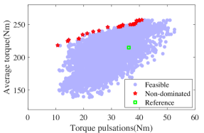
(a) NSGA-II (7,500 evals).

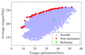
(b) NSGA-II-WR (7,500 evals).

Figure 5: Objective space illustrating dominated and non-dominated (Pareto) solutions obtained with all runs combined of NSGA-II and NSGA-II-WR algorithms in 5(a) and 5(b), respectively. All feasible solutions obtained since the start of a specific run are shown in blue color.

5.2 Convergence Analysis With and Without Surrogates

Although surrogate-assisted optimization is known to find the Pareto-optimal front quicker than other methods, it is also sensitive to (model and optimization-related) hyperparameters. In this article, the following three hyperparameters are varied to analyze the performance of the proposed optimization method with surrogates.

• $N$: Number of ESEs in each iteration

• $k$: Number of surrogate optimization generations for exploitation

• $N^{\texttt{DOE}}$: Number of initial design of experiments

The complete setup and results of this parametric study and some important observations are included in the supplementary document for reference. Based on this study, $N$ = 10, $k$ = 35, and $N^{\texttt{DOE}}$ = 60, is identified as the best parameter setting out of the analyzed configurations. For the remainder of this article, the corresponding surrogate-assisted optimization configuration is referred to as NSGA-II-WR-SA, and its results are compared with those obtained with NSGA-II-WR. A comparison of the two Pareto-optimal fronts clearly shows that NSGA-II-WR-SA outperforms NSGA-II-WR, as shown in Figure 6(a). It should be noted that the compared Pareto-optimal fronts are obtained by combining all five runs for both algorithms, NSGA-II-WR and NSGA-II-WR-SA, respectively. To understand the convergence of each optimization method, the design space of the two Pareto-optimal sets are visualized by a parallel coordinates plot (PCP) (see Figure 6(b)). Each vertical axis in the PCP represents the normalized variable $x_{i}$ with its lower and upper bounds as 0 and 1, respectively, and each horizontal line represents a solution. The design space of the two Pareto-optimal sets shows that most of the variables have converged to an optimal value with NSGA-II-WR-SA, whereas, with NSGA-II-WR, some of the variables still have significant variations with further scope for improvement. These observations validate the effectiveness of the incorporation of surrogates by demonstrating the improvement in the convergence. Moreover, it should be noted that while NSGA-II-WR has used 7,500 evaluations in this experiment, NSGA-II-WR-SA has converged to a better set of solutions with a solution evaluation budget of only 1,000. As explained in the previous section, surrogates are utilized to look $k$ generations (here $k=35$) into the future to generate $N$ number of infill solutions in each optimization cycle, which leads to better convergence. A comparison of individual runs included in the supplementary document further demonstrates the superiority of NSGA-II-WR-SA over NSGA-II-WR. Additionally, a discussion on the performance of surrogates and exploration of search space included in the supplementary document shows that the convergence with surrogates depends on the complexity of the objective functions under consideration.

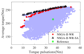
(a)

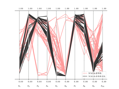
(b)

Figure 6: Comparison of objective space with Pareto-optimal fronts and normalized design space of Pareto optimal sets in 6(a) and 6(b) respectively. Pareto-optimal sets are obtained by combining all runs completed with the optimization methods, NSGA-II-WR and NSGA-II-WR-SA, respectively.

5.3 Analysis of Pareto-Optimal Solutions

The design space of the Pareto-optimal set obtained with NSGA-II-WR-SA is investigated to gain insights into the electric machine design (see Figure 6(b)). In general, while machine flux linkages affect the average torque, magnet pole arc and material saturation control the torque pulsations. Nevertheless, some critical observations are listed below.

• Most of the Pareto-optimal solutions have larger values of magnet width ($x_{3}$), which results in more magnet flux linkage and average torque. Larger magnet width also results in smaller q-axis width ($x_{6}$).

• Most solutions also have larger values of slot height ($x_{7}$) and slot width ($x_{8}$) and, therefore, slot cross-section. A larger slot cross-section area results in more winding space, which translates to higher allowable excitation current and an increase in average torque.

• Reduction in bridge height ($x_{5}$) directly increases the air-gap flux density, which increases average torque.

• Magnet pole arc is directly proportional to magnet width ($x_{3}$) and angle between the magnets ($x_{4}$), and an increase in magnet pole arc seems to reduce pulsations.

• Material saturation is a nonlinear behavior observed in magnetic materials, such as electrical steel, introducing saturation harmonics in magnetic flux density. While a larger slot cross-section increases average torque through more excitation current, it also increases magnetic material saturation, leading to more torque pulsations.

• Lastly, the height and width of slot opening, $x_{9}$ and $x_{10}$, which are responsible for slot harmonics, have converged to the lower end of the variable range.

5.4 Selection of Preferred Solutions

The selection of an electric machine design is primarily application-dependent. One approach could be to use a scalarized function yielding a single optimal solution (Islam, Bonthu, and Choi 2015). However, proper scalarization of objectives is a difficult task. Scalarization also does not offer the possibility of analyzing trade-offs observed for multiple objectives. Moreover, optimizing all objectives likely produces a Pareto-optimal front which is harder to interpret and gain insights into the electric machine design. This article uses two approaches to select the preferred solutions: (1) a domain-specific a posteriori MCDM method that involves machine expertise and (2) a trade-off analysis of the Pareto-optimal set to identify and choose the solutions with the highest trade-off. Pareto-optimal solutions obtained from combined runs of NSGA-II-WR and NSGA-II-WR-SA optimization methods are used in both approaches.

5.4.1 Domain Specific A Posteriori MCDM Method

For a domain-specific a posteriori MCDM method, three performance measures, in addition to the two objective functions defined in (1), are used to select preferred solutions from the Pareto-optimal set.

• Total harmonic distortion of noload back emf (THDV)

• Peak of fundamental of back emf (F-BEMF)

• Magnet utilization factor (MUF)

Since THDV is directly proportional to noise, vibration, and harshness (NVH) during the operation of an electric machine, a solution with low THDV is desirable. Conversely, F-BEMF instead introduces a trade-off as a high F-BEMF increases average torque, but it also leads to a reduced speed range. Lastly, a design with high MUF is desirable, where MUF is defined as the ratio of average torque to PM volume. A primary screening based on THDV of Pareto-optimal solutions shows that the solutions lying in the bottom region of the Pareto-front must be avoided as they have more than 30% THDV, as shown in Figure 7(a). Since the remaining Pareto-optimal solutions have similar THDV (10-14%), it is easier to select solutions based on the remaining performance measures. Consequently, three preferred solutions, 1, 2, and 3, highlighted in Figure 7(a), are selected after further evaluation. The basis of the selection of the solutions is as follows.

• Solution 1: maximum average torque

• Solution 2: maximum MUF

• Solution 3: minimum pulsation and F-BEMF

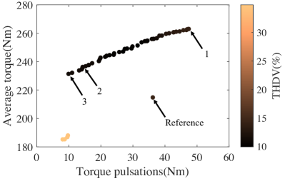
(a)

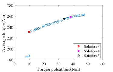
(b)

Figure 7: Objective space highlighting the selected solutions using the a posteriori MCDM method and trade-off analysis in 7(a) and 7(b), respectively.

5.4.2 Trade-Off Calculation Using Objective Functions

A trade-off analysis of the Pareto-optimal front is an effective method to select preferred solutions without domain expertise. In this article, for a particular solution ($\mathbf{x}^{(i)}$), trade-off is calculated using (2) on the neighborhood of points, represented by $B(\mathbf{x}^{(i)})$. The term $\sum^{M}_{m=1}\{1|c_{m}>d_{m}\}$ calculates the number of $m$’s (out of $M$) for which the condition $c_{m}>d_{m}$ is valid. In this article, the complete Pareto-optimal set obtained from NSGA-II-WR and NSGA-II-WR-SA, as explained previously, defines the neighborhood of points, $B(\mathbf{x}^{(i)})$. For trade-off calculation, only two objective functions defined in (1) are used and solutions with high trade-off values are desired.

$$\begin{split}\texttt{Avg.Loss}(\mathbf{x}^{(i)},\mathbf{x}^{(j)})&=\frac{\sum^{M}_{m=1}\max\left(0,f_{m}(\mathbf{x}^{(j)})-f_{m}(\mathbf{x}^{(i)})\right)}{\sum^{M}_{m=1}\{1|f_{m}(\mathbf{x}^{(j)})>f_{m}(\mathbf{x}^{(i)})\}},\\[5.69054pt] \texttt{Avg.Gain}(\mathbf{x}^{(i)},\mathbf{x}^{(j)})&=\frac{\sum^{M}_{m=1}\max\left(0,f_{m}(\mathbf{x}^{(i)})-f_{m}(\mathbf{x}^{(j)})\right)}{\sum^{M}_{m=1}\{1|f_{m}(\mathbf{x}^{(i)})>f_{m}(\mathbf{x}^{(j)})\}},\\[5.69054pt] \texttt{Trade-off}(\mathbf{x}^{(i)})&=\max^{|B(\mathbf{x}^{(i)})|}_{j=1}\frac{\texttt{Avg.Loss}(\mathbf{x}^{(i)},\mathbf{x}^{(j)})}{\texttt{Avg.Gain}(\mathbf{x}^{(i)},\mathbf{x}^{(j)})}.\end{split}$$ (2)

After performing the trade-off calculation, three solutions with the highest trade-offs, Solution 3, 4, and 5, are identified from the combined Pareto-optimal set, as shown in Figure 7(b). The trade-off values of the selected solutions are given below. Interestingly, Solution 3 is picked again with the highest trade-off value. Additionally, since Solutions 4 and 5 offer a relatively smaller trade-off value compared to Solution 3, they are not considered in the rest of the discussion.

• Solution 3: highest trade-off value (114.99)

• Solution 4: $2^{nd}$ highest trade-off value (50.79)

• Solution 5: $3^{rd}$ highest trade-off value (35.07)

5.4.3 Performance comparison of selected solutions

Performance details of the selected solutions and the reference design are given in Table 5.4.3. Further insights into the performance of these solutions can be gained by analyzing the design space, as shown in Figure 8(a). Some essential observations highlighting the trade-off among selected solutions are as follows.

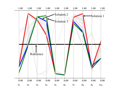
(a)

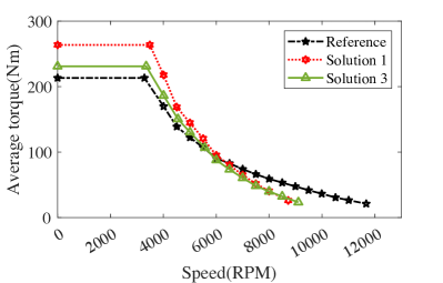
(b)

Figure 8: Selected Pareto-optimal solutions are highlighted in normalized design space in 8(a). Torque-speed curve of reference design and solutions 1 and 3 is shown in 8(b).

Performance comparison of five preferred solutions found using domain specific a posteriori MCDM method and trade-off analysis. Preferred values are highlighted in bold for the three solutions. Solution Avg torque Pulsations THDV MUF F-BEMF (Nm) (Nm) (%) (Nm/mm³) (V) 1 $\mathbf{263.0374}$ 47.4060 14.1263 0.0290 248.2401 2 235.5986 14.2488 $\mathbf{11.2982}$ $\mathbf{0.0308}$ 236.7291 3 231.3853 $\mathbf{9.9186}$ 11.5016 0.0304 $\mathbf{234.4451}$ Reference 214.7760 36.1846 14.4093 0.0330 209.2622

• Although Solution 1 provides maximum average torque; it also has the maximum amplitude of pulsations and F-BEMF. Both these characteristics can be explained by larger magnet thickness ($x_{2}$), slot height ($x_{7}$), slot width ($x_{8}$), and slot opening height and width ($x_{9}$ and $x_{10}$).

• Solutions 2 and 3 perform quite similarly in all aspects, with slight variations observed in average torque and torque pulsations. This variation is caused by the different angles between magnets ($x_{4}$) observed for the two solutions.

• All selected solutions have a larger F-BEMF value compared to the reference design. In other words, they have a lower speed range. The relation between F-BEMF and the maximum achievable speed is illustrated in Figure 8(b). With further increase in speeds, one would observe that torque produced by Solution 1 drops to zero more quickly compared to Solution 3. Since Solutions 2 and 3 have similar F-BEMF, their torque/speed profiles are also expected to be similar.

• A comparison of the magnetic flux density plots of Solutions 1, 2, and 3 at corresponding rated operating conditions reveals that Solution 1 suffers from higher saturation in stator teeth, back iron, and rotor steel close to magnet edges (see Figure 9).

Based on this in-depth discussion, one should select Solution 1 for an application with a high average torque requirement. If the focus is more on a smooth operation with a high-speed range, Solution 2 or 3 should be chosen. It is also worth mentioning that while the trade-off analysis can pick Solution 3, it does not pick Solution 2 with the highest MUF, but can be selected by utilizing domain expertise. Ultimately, selecting a single solution out of a Pareto-optimal set is a difficult task that can often be alleviated using the machine designer’s experience.

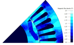
(a) Solution 1.

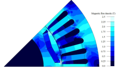
(b) Solution 2.

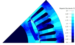
(c) Solution 3.

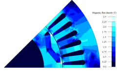
(d) Reference design.

Figure 9: Magnetic flux density plots of Solutions 1, 2, 3 and reference design at rated operation.

6 Conclusion

This article has investigated a bi-objective electric machine design optimization problem with geometric constraints. While the geometric constraints are evaluated using analytical expressions, the objective functions require costly finite element analysis, leading to a mixed computational expensive optimization problem. The proposed method has utilized a repair operator to handle inexpensive constraints and surrogate models to predict expensive objectives. Both concepts have been integrated into the well-known evolutionary multi-objective optimization (EMO) algorithm NSGA-II. Results have indicated an improved quality of the Pareto-optimal solution set using the repair operator and thus the effectiveness of ensuring feasibility during optimization. Moreover, the surrogate incorporation has been analyzed in-depth and shown to be critical for improving efficiency. First, surrogate related parameters have been investigated by performing a sequential parametric study, examining the number of infill solutions in each generation ($N$), the number of generations for exploiting the surrogate model ($k$), and the number of the initial design of experiments ($N^{\texttt{DOE}}$). The parametric study has provided a suitable configuration for solving this electric machine design problem. Results have validated the superiority of incorporating surrogates by improving the algorithm’s convergence with a small number of expensive evaluations.

The ultimate goal of an optimization process is to reach an optimal solution that can be implemented successfully. Unlike many other applied multi-objective optimization studies, this article has presented a domain-specific a posteriori MCDM approach focusing on machine cost, noise, vibration, and harshness (NVH), and speed range of the electric machine to choose a single preferred solution. The presented a-posteriori selection approach has identified the trade-off offered by different Pareto-optimal solutions and facilitated selecting a handful of optimized electric machine designs. Additionally, trade-off calculations based on objective functions have been performed to select preferred solutions, thereby helping the user identify a few critical designs from a large search space.

Future research shall be conducted on an approach to perform parameter tuning automatically. Moreover, this article has explored the effectiveness of surrogates by analyzing the accuracy of objective value predictions. It has been observed that nonlinear objective functions may delay the algorithm’s convergence. In electric machines, the nonlinear behavior of magnetic material is dependent on the operating point. A space-filling sampling technique, which systematically explores the entire objective space, could be an effective way to account for this non-linearity before optimization. However, in real-world optimization problems, such as electric machine design, prior information about objective space is usually not available. This can be the subject of future research in the electric machine community. Integrating a repair operator and surrogate models into an EMO algorithm has shown promising results for optimizing electric machine designs. The proposed concepts’ generalizability shall be further explored by incorporating them into other EMO methods. Moreover, more application problems having a computationally mixed expensive nature need to be investigated. Nevertheless, this study has clearly shown the advantage of using a flexible EMO algorithm with efficient handling of constraints and the use of surrogates for expensive evaluation procedures to discover a diverse set of high-performing designs. The study has also revealed a set of key design principles common to multiple high-performing designs for enhancing knowledge about the problem and demonstrated the use of MCDM approaches to choose one or a few preferred solutions for implementation. The complete optimization-cum-decision-making on a complex electric motor design problem demonstrated in this study should pave the way for applying similar procedures in other engineering design optimization tasks.

7 Data Availability Statement

The data that support the findings of this study are available from the corresponding author upon reasonable request.

8 Disclosure Statement

No potential competing interest was reported by the authors.

References

- Altair (2019) Altair. 2019. Altair FluxMotor (Version 2019.1.1). Altair Engineering Inc. Availablefromhttps://www.altair.com/fluxmotor/.
- Bianchi and Bolognani (1998) Bianchi, N., and S. Bolognani. 1998. “Design optimisation of electric motors by genetic algorithms.” IEE Proceedings - Electric Power Applications 145: 475–483(8). https://digital-library.theiet.org/content/journals/10.1049/ip-epa\_19982166.
- Blank and Deb (2021) Blank, J., and K. Deb. 2021. “Constrained bi-objective surrogate-assisted optimization of problems with heterogeneous evaluation times: Expensive objectives and inexpensive constraints.” In Evolutionary multi-criterion optimization, edited by Hisao Ishibuchi, Qingfu Zhang, Ran Cheng, Ke Li, Hui Li, Handing Wang, and Aimin Zhou, 257–269. Springer International Publishing.
- Deb et al. (2019) Deb, K., R. Hussein, P. C. Roy, and G. Toscano-Pulido. 2019. “A taxonomy for metamodeling frameworks for evolutionary multiobjective optimization.” IEEE Transactions on Evolutionary Computation 23 (1): 104–116.
- Deb et al. (2002) Deb, K., A. Pratap, S. Agarwal, and T. Meyarivan. 2002. “A fast and elitist multiobjective genetic algorithm: NSGA-II.” IEEE Transactions on Evolutionary Computation 6 (2): 182–197.
- Degano et al. (2016) Degano, M., M. Di Nardo, M. Galea, C. Gerada, and D. Gerada. 2016. “Global design optimization strategy of a synchronous reluctance machine for light electric vehicles.” In 8th IET International Conference on Power Electronics, Machines and Drives (PEMD 2016), 1–5.
- Duan, Harley, and Habetler (2009) Duan, Y., R. G. Harley, and T. G. Habetler. 2009. “Comparison of particle swarm optimization and genetic algorithm in the design of permanent magnet motors.” 2009 IEEE 6th International Power Electronics and Motion Control Conference, IPEMC ’09 3: 822–825.
- Duan and Ionel (2013) Duan, Yao, and Dan M. Ionel. 2013. “A review of recent developments in electrical machine design optimization methods with a permanent-magnet synchronous motor benchmark study.” IEEE Transactions on Industry Applications 49 (3): 1268–1275.
- Hardy (1971) Hardy, Rolland L. 1971. “Multiquadric equations of topography and other irregular surfaces.” Journal of Geophysical Research (1896-1977) 76 (8): 1905–1915. Accessed 2020-10-06. https://doi.org/10.1029/JB076i008p01905.
- Hooke and Jeeves (1961) Hooke, Robert, and T. A. Jeeves. 1961. ““ Direct Search” Solution of Numerical and Statistical Problems.” J. ACM 8: 212–229.
- Ionel and Popescu (2009) Ionel, Dan M., and Mircea Popescu. 2009. “Finite element surrogate model for electric machines with revolving field — application to IPM motors.” In 2009 IEEE Energy Conversion Congress and Exposition, 178–186.
- Islam, Bonthu, and Choi (2015) Islam, Md. Zakirul, Sai Sudheer Reddy Bonthu, and Seungdeog Choi. 2015. “Obtaining optimized designs of multi-phase PMa-SynRM using lumped parameter model based optimizer.” In 2015 IEEE International Electric Machines Drives Conference (IEMDC), 1722–1728.
- Jolly, Jabbar, and Qinghua (2005) Jolly, L., M.A. Jabbar, and Liu Qinghua. 2005. “Design optimization of permanent magnet motors using response surface methodology and genetic algorithms.” IEEE Transactions on Magnetics 41 (10): 3928–3930.
- Khoshoo et al. (2021) Khoshoo, Bhuvan, Julian Blank, Thang Pham, Kalyanmoy Deb, and Shanelle Foster. 2021. “Optimized Electric Machine Design Solutions with Efficient Handling of Constraints.” In 2021 IEEE Symposium Series on Computational Intelligence (SSCI), 1–8.
- Krige (1951) Krige, D. G. 1951. “A statistical approach to some basic mine valuation problems on the Witwatersrand, by D.G. Krige, published in the Journal, December 1951 : introduction by the author.” .
- Mirzaeian et al. (2002) Mirzaeian, B., M. Moallem, V. Tahani, and C. Lucas. 2002. “Multiobjective optimization method based on a genetic algorithm for switched reluctance motor design.” IEEE Transactions on Magnetics 38 (3): 1524–1527.
- Pellegrino and Cupertino (2010a) Pellegrino, G., and F. Cupertino. 2010a. “FEA-based multi-objective optimization of IPM motor design including rotor losses.” In 2010 IEEE Energy Conversion Congress and Exposition, 3659–3666.
- Pellegrino and Cupertino (2010b) Pellegrino, G., and F. Cupertino. 2010b. “IPM motor rotor design by means of FEA-based multi-objective optimization.” In 2010 IEEE International Symposium on Industrial Electronics, 1340–1346.
- Pellegrino, Cupertino, and Gerada (2015) Pellegrino, Gianmario, Francesco Cupertino, and Chris Gerada. 2015. “Automatic Design of Synchronous Reluctance Motors Focusing on Barrier Shape Optimization.” IEEE Transactions on Industry Applications 51 (2): 1465–1474.
- Ramarathnam, Desai, and Rao (1973) Ramarathnam, R., B. G. Desai, and V. Subba Rao. 1973. “A Comparative Study of Minimization Techniques for Optimization of Induction Motor Design.” IEEE Transactions on Power Apparatus and Systems PAS-92 (5): 1448–1454.
- Singh et al. (1983) Singh, Bhim, B. P. Singh, S. S. Murthy, and C. S. Jha. 1983. “Experience in Design Optimization of Induction Motor Using ’SUMT’ Algorithm.” IEEE Transactions on Power Apparatus and Systems PAS-102 (10): 3379–3384.
- Sizov, Ionel, and Demerdash (2012) Sizov, Gennadi Y., Dan M. Ionel, and Nabeel A. O. Demerdash. 2012. “Modeling and Parametric Design of Permanent-Magnet AC Machines Using Computationally Efficient Finite-Element Analysis.” IEEE Transactions on Industrial Electronics 59 (6): 2403–2413.
- Song et al. (2018) Song, Juncai, Jiwen Zhao, Fei Dong, Jing Zhao, Zhe Qian, and Qian Zhang. 2018. “A Novel Regression Modeling Method for PMSLM Structural Design Optimization Using a Distance-Weighted KNN Algorithm.” IEEE Transactions on Industry Applications 54 (5): 4198–4206.
- Stipetic, Miebach, and Zarko (2015) Stipetic, Stjepan, Werner Miebach, and Damir Zarko. 2015. “Optimization in design of electric machines: Methodology and workflow.” In 2015 Intl Aegean Conference on Electrical Machines Power Electronics (ACEMP), 2015 Intl Conference on Optimization of Electrical Electronic Equipment (OPTIM) 2015 Intl Symposium on Advanced Electromechanical Motion Systems (ELECTROMOTION), 441–448.
- Sudhoff et al. (2005) Sudhoff, Scott D., James Cale, Brandon Cassimere, and Mike Swinney. 2005. “Genetic algorithm based design of a permanent magnet synchronous machine.” 2005 IEEE International Conference on Electric Machines and Drives 1011–1019.
- Taran, Ionel, and Dorrell (2018) Taran, Narges, Dan M. Ionel, and David G. Dorrell. 2018. “Two-Level Surrogate-Assisted Differential Evolution Multi-Objective Optimization of Electric Machines Using 3-D FEA.” IEEE Transactions on Magnetics 54 (11): 1–5.
- Žarko, Ban, and Lipo (2005) Žarko, Damir, Drago Ban, and Thomas A. Lipo. 2005. “Design optimization of Interior Permanent Magnet (IPM) motors with maximized torque output in the entire speed range.” 2005 European Conference on Power Electronics and Applications 2005.
- Zhang et al. (2013) Zhang, Peng, Gennadi Y. Sizov, Dan M. Ionel, and Nabeel A.O. Demerdash. 2013. “Design optimization of spoke-type ferrite magnet machines by combined design of experiments and differential evolution algorithms.” In 2013 International Electric Machines Drives Conference, 892–898.
- Zitzler, Brockhoff, and Thiele (2007) Zitzler, Eckart, Dimo Brockhoff, and Lothar Thiele. 2007. “The Hypervolume Indicator Revisited: On the Design of Pareto-compliant Indicators Via Weighted Integration.” In Evolutionary Multi-Criterion Optimization, edited by Shigeru Obayashi, Kalyanmoy Deb, Carlo Poloni, Tomoyuki Hiroyasu, and Tadahiko Murata, Berlin, Heidelberg, 862–876. Springer Berlin Heidelberg.