Three-dimensional microstructure generation using generative adversarial neural networks in the context of continuum micromechanics

Abstract

Multiscale simulations are demanding in terms of computational resources. In the context of continuum micromechanics, the multiscale problem arises from the need of inferring macroscopic material parameters from the microscale. If the underlying microstructure is explicitly given by means of $\mu$CT-scans, convolutional neural networks can be used to learn the microstructure-property mapping, which is usually obtained from computational homogenization. The CNN approach provides a significant speedup, especially in the context of heterogeneous or functionally graded materials. Another application is uncertainty quantification, where many expansive evaluations are required. However, one bottleneck of this approach is the large number of training microstructures needed.

This work closes this gap by proposing a generative adversarial network tailored towards three-dimensional microstructure generation. The lightweight algorithm is able to learn the underlying properties of the material from a single $\mu$CT-scan without the need of explicit descriptors. During prediction time, the network can produce unique three-dimensional microstructures with the same properties of the original data in a fraction of seconds and at consistently high quality.

spacing=nonfrench [label1] organization=Institute for Computational Modeling in Civil Engineering, Technical University of Braunschweig, addressline=Pockelsstr. 3, city=Braunschweig, postcode=38106, country=Germany

1 Introduction

Modern composite materials in aerospace, automotive, civil and mechanical engineering consist of multiple constituents, which induce macroscopic properties by means of their microstructure [1]. This introduces a multi-scale problem understood as inferring quantities of interest on the macro-scale by means of microscopic entities [2]. To this end, computational homogenization algorithms aim towards calculation of effective material properties by calculating quantities of interest on the micro-scale and projecting them to higher scales [3]. This is typically carried out using numerical algorithms like the finite element method (FEM) or fast Fourier transform (FFT) based methods. While mostly leading to more precise result than analytical homogenization methods, a major drawback is the large computational effort.

A new direction in the field of engineering is opened up by machine learning algorithms [4]. Especially, the homogenization procedure can be accelerated by artificial neural networks (ANN), which are able to approximate arbitrary Borel measurable functions [5]. Application of ANNs to deterministic full-field homogenization can be found in [6, 7, 8, 9] and in the context of uncertainty quantification in [10, 11]. The concept paper [12] provides a low-threshold overview of the topic. To train an ANN for homogenization, training data is needed. In the case of microstructures, these are usually obtained synthetically or from $\mu$CT-scans [13]. Although the material characteristics are more realistic for $\mu$CT-scans than for computed microstructures [14], the available amount of image data usually is severely limited, as a single $\mu$CT-scan lasts several hours and hence only a couple of them are available at reasonable cost [15]. Even though several hundreds of microstructures can be extracted from these, this is typically not enough for modern ANNs, which need thousands of unique three-dimensional images during training [16]. There exist stochastic microstructure generation approaches, such as [17] [18], [19], [20], [21], which use descriptors to model the characteristics of the morphology. These descriptors are often non-trivial and induce a human bias towards the properties of the microstructure.

To circumvent this problem, ANNs can be used to synthetically generate microstructures drawn directly from the underlying generating distribution of the $\mu$CT-scans. These special kind of ANNs are called generative adversarial networks (GAN). They were originally introduced for two-dimensional images in [22], where two ANNs take part in a two-player game of generating synthetic images and trying to discriminate them from a set of real images, respectively. When the Nash equilibrium [23] in this two-player game is reached, the discriminating ANN cannot distinguish between real and synthetic images anymore, as the quality of the generated ones is similar to the original. The basic GAN formulation was improved in succeeding works to overcome problems like training instability utilizing a Wasserstein distance used in optimal transport [24, 25] leading to Wasserstein GANs [26, 27, 28]. The current state of the art topologies are the StyleGAN models from NVIDIA and its successors [29, 30, 31]. For a recent overview about standard GAN topologies see [32]. GANs are successfully engaged in three-dimensional settings like high-energy physics [33] and especially in medical imaging domains such as brain image reconstruction [34] and biomedical image generation [35].

In the context of microstructure generation, GANs were used on plane porous material and rock $\mu$CT-scans using a two-dimensional StyleGAN architecture [36]. In [37], a WGAN was used alongside physical constraints on the generated two-dimensional microstructures of a synthetic dataset. Two-dimensional microstructures of steel were produced in [38]. In the three-dimensional regime, the porous media flow properties of generated microstructures were investigated in [39], whereas in [40] and [41] solid oxide fuel cell electrodes for electrochemistry simulations where synthesized.

To the best of the authors knowledge, no attempts were made in applying the GAN approach in the context of solid micro-mechanical homogenization. Furthermore, state of the art GANs like StyleGAN have many parameters and take substantial effort to train, as in the case of [40], especially in the three-dimensional regime. The above mentioned studies often base their network topology on ad-hoc assumptions or fail to explain their choices. Important effects like the number of samples needed in practical applications, where only a limited amount of micrographs are available, were not investigated. To close these gaps, the present study therefore aims towards the following key contributions:

• Three-dimensional GAN for micromechanics: A GAN for three-dimensional microstructures based on $\mu$CT-scans is presented. The performance is evaluated by computational homogenization based on FFT as well as different microstructural descriptors.

• Lightweight network topology: The presented GAN utilizes several techniques to achieve good results tailored towards microstructure generation while avoiding unnecessary complexity. The GAN can be trained on a single workstation.

• Transfer to real-world applications: Numerical experiments considering important influencing factors on real-world applicability such as network size and number of training samples are carried out on two different microstructures, including a wood-plastic composite $\mu$CT-scan.

The remainder of this paper is structured as follows. In Section 2, a theoretical overview of the most important aspects of this work are given. In detail, Section 2.1 introduces ANN and Section 2.2 the main ideas of GANs. Computational homogenization is briefly summarized in Section 2.3. The proposed GAN is introduced and explained in Section 3. Then, two microstructures are investigated in numerical examples. First, in Section 4, a challenging three-dimensional microstructure of spherical inclusions is considered. Here, several hyperparameters and techniques are discussed, such as overfitting effects and topology choices. The resulting homogenized properties of the baseline and the synthetic microstructures are compared. Second, in Section 5, a $\mu$CT-scan of a wood-plastic composite is examined. The results of this work are discussed in Section 6, moreover an outlook is given. Two appendices deal with the applicability of geometrical and physical constraints in A and B, respectively, for GANs in the context of microstructure generation and are intended for researchers who may want to continue research along the direction of this paper.

2 Preliminaries

This section introduces the basic notations of ANNs, GANs and computational homogenization, which are essential for the developments in Section 3.

2.1 Artificial neural networks

An ANN is a parametrized, nonlinear function composition. By the universal function approximation theorem [5], arbitrary Borel measurable functions can be approximated by ANN. There are several different formulations for ANN, which can be found in standard references such as [42, 43, 44, 45, 46]. Following [47], most ANN formulations can be unified. An ANN $\mathcal{N}$ is a function from an input space $\mathbb{R}^{d_{x}}$ to an output space $\mathbb{R}^{d_{y}}$, defined by a composition of nonlinear functions $\bm{h}^{(l)}$, such that

$$\mathcal{N}:\mathbb{R}^{d_{x}} \to\mathbb{R}^{d_{y}}$$

$$\bm{x} \mapsto\mathcal{N}(\bm{x})=\bm{h}^{(l)}\circ\ldots\circ\bm{h}^{(0)}=\bm{y},\quad l=1,\ldots,n_{L}.$$ ((1))

Here, $\bm{x}$ denotes an input vector of dimension $d_{x}$ and $\bm{y}$ an output vector of dimension $d_{y}$. The nonlinear functions $\bm{h}^{(l)}$ are called layers and define an $l$-fold composition, mapping input vectors to output vectors. Consequently, the first layer $\bm{h}^{(0)}$ is defined as the input layer and the last layer $\bm{h}^{(n_{L})}$ as the output layer, such that

$$\bm{h}^{(0)}=\bm{x}\in\mathbb{R}^{d_{x}},\qquad\bm{h}^{(n_{L})}=\bm{y}\in\mathbb{R}^{d_{y}}.$$ ((2))

The layers $\bm{h}^{(l)}$ between the input and output layer, called hidden layers, are defined as

$$\bm{h}^{(l)}\mathchoice{\mathrel{\hbox{\hbox to0.0pt{$-$\hss}$<$}}}{\mathrel{\hbox{\hbox to0.0pt{$-$\hss}$<$}}}{\mathrel{\hbox{\hbox to0.0pt{$\scriptstyle-$\hss}$\scriptstyle<$}}}{\mathrel{\hbox{\hbox to0.0pt{$\scriptscriptstyle-$\hss}$\scriptscriptstyle<$}}}\bm{h}_{\bullet}^{(l)}=\left\{h_{\bullet,\eta}^{(l)},\;\eta=1,\ldots,n_{u}\right\},\qquad h_{\bullet,\eta}^{(l)}=\varphi^{(l)}\circ\;\phi^{(l)}\left(\bm{W}^{(l)}_{\eta}\bullet\bm{h}^{(l-1)}\right),$$ ((3))

where $h_{\bullet,\eta}^{(l)}$ is the $\eta$-th neural unit of the $l$-th layer $\bm{h}_{\bullet}^{(l)}$ and $n_{u}$ is the total number of neural units per layer, while $\bullet$ denotes a product. Following the notation in [48], the symbol $\mathchoice{\mathrel{\hbox{\hbox to0.0pt{$-$\hss}$<$}}}{\mathrel{\hbox{\hbox to0.0pt{$-$\hss}$<$}}}{\mathrel{\hbox{\hbox to0.0pt{$\scriptstyle-$\hss}$\scriptstyle<$}}}{\mathrel{\hbox{\hbox to0.0pt{$\scriptscriptstyle-$\hss}$\scriptscriptstyle<$}}}$ denotes an abbreviation of a tuple of mathematical objects $(\mathcal{O}_{1},\mathcal{O}_{2},...)$, such that $\mathcal{O}\mathchoice{\mathrel{\hbox{\hbox to0.0pt{$-$\hss}$<$}}}{\mathrel{\hbox{\hbox to0.0pt{$-$\hss}$<$}}}{\mathrel{\hbox{\hbox to0.0pt{$\scriptstyle-$\hss}$\scriptstyle<$}}}{\mathrel{\hbox{\hbox to0.0pt{$\scriptscriptstyle-$\hss}$\scriptscriptstyle<$}}}(\mathcal{O}_{1},\mathcal{O}_{2},...)$. In Eq. (3), the details of type-specific layers $\bm{h}_{\bullet}^{(l)}$ are gathered in general layers $\bm{h}^{(l)}$ from Eq. (1). The specification follows from the $\bullet$-operator, which denotes the operation between the weight vector $\bm{W}_{\eta}^{(l)}$ of the $\eta$-th neural unit in the $l$-th layer $\bm{h}_{\bullet}^{(l)}$ and the output of the preceding layer $\bm{h}_{\bullet}^{(l-1)}$, where the bias term is absorbed [44]. If $\bullet$ is the ordinary matrix multiplication $\bullet=\cdot$, then the layer $\bm{h}_{\cdot}^{(l)}$ is called dense layer. If $\bullet$ is the convolution or cross-correlation operation $\bullet=\star$, then the layer $\bm{h}_{\star}^{(l)}$ is called convolutional layer. In the context of convolutional layers, the weight vector $\bm{W}_{\eta}^{(l)}$ from Eq. (1) is also called filter, such that $n_{u}=n_{f}$ denotes the number of filters. Furthermore, $\phi^{(l)}:\mathbb{R}\to\mathbb{R}$ is a nonlinear activation function and $\varphi^{(l)}$ is a function of the previous layer, such that $\varphi^{(l)}:\bm{h}^{(l-1)}\mapsto\varphi^{(l)}(\bm{h}^{(l-1)})$. If $\varphi^{(l)}$ is the identity function, the layer $\bm{h}^{(l)}$ is called a feed forward layer. Otherwise, the layer $\bm{h}^{(l)}$ is called residual layer. All weight vectors $\bm{W}_{\eta}^{(l)}$ of all layers $\bm{h}^{(l)}$ can be gathered in a single expression, such that

$$\bm{\theta}=\left\{\bm{W}_{\eta}^{(l)}\right\},$$ ((4))

where $\bm{\theta}$ inherits all parameters of the ANN $\mathcal{N}(\bm{x})$ from Eq. (1). Consequently, the notation $\mathcal{N}(\bm{x};\bm{\theta})$ emphasizes the dependency of the outcome of an ANN on the input on the one hand and the current realization of the weights on the other hand. The specific combination of layers $\bm{h}_{\bullet}^{(l)}$ from Eq. (3), neural units $h_{\bullet,\eta}^{(l)}$ and activation functions $\phi^{(l)}$ from Eq. (3) is called topology of the ANN $\mathcal{N}(\bm{x};\bm{\theta})$. The weights $\bm{\theta}$ from Eq. (4) are typically found by gradient-based optimization with respect to a task-specific loss function [43].

2.2 Generative adversarial neural networks

A GAN consists of two competing ANN from Eq. (1), namely the generator $\mathcal{G}\mathchoice{\mathrel{\hbox{\hbox to0.0pt{$-$\hss}$<$}}}{\mathrel{\hbox{\hbox to0.0pt{$-$\hss}$<$}}}{\mathrel{\hbox{\hbox to0.0pt{$\scriptstyle-$\hss}$\scriptstyle<$}}}{\mathrel{\hbox{\hbox to0.0pt{$\scriptscriptstyle-$\hss}$\scriptscriptstyle<$}}}\mathcal{N}(\bm{x};\bm{\theta})=\mathcal{N}_{\mathcal{G}}(\bm{z};\bm{\theta}_{\mathcal{G}})$ and the discriminator (sometimes called critic) $\mathcal{D}\mathchoice{\mathrel{\hbox{\hbox to0.0pt{$-$\hss}$<$}}}{\mathrel{\hbox{\hbox to0.0pt{$-$\hss}$<$}}}{\mathrel{\hbox{\hbox to0.0pt{$\scriptstyle-$\hss}$\scriptstyle<$}}}{\mathrel{\hbox{\hbox to0.0pt{$\scriptscriptstyle-$\hss}$\scriptscriptstyle<$}}}\mathcal{N}(\bm{x};\bm{\theta})=\mathcal{N}_{\mathcal{D}}(\bm{I};\bm{\theta}_{\mathcal{D}})$. The goal of the GAN approach is to create synthetic images using the generator which have the same properties as original images from a dataset. To this end, the generator $\mathcal{G}$ maps random input vectors $\bm{z}$ from a $d_{x}=d_{Z}$-dimensional input space $\mathcal{Z}\subset\mathbb{R}^{d_{x}}=\mathbb{R}^{d_{Z}}$ called latent space to images $\bm{I}$ in the $d_{y}=d_{I}$-dimensional output synthetic image space $\mathcal{I}\subset\mathbb{R}^{d_{y}}=\mathbb{R}^{d_{I}}$, such that

$$\mathcal{G}:\mathcal{Z}\subset\mathbb{R}^{d_{Z}} \to\mathcal{I}\subset\mathbb{R}^{d_{I}}$$

$$\bm{z} \mapsto\mathcal{G}(\bm{z})=\bm{I}.$$ ((5))

The discriminator $\mathcal{D}$ aims to distinguish between synthetic images $\bm{I}$ and real images $\bm{I}_{\text{data}}\in\mathbb{D}\subset\mathcal{I}_{\text{data}}$ taken from a dataset $\mathbb{D}$, a subset of the $d_{I}$-dimensional real image space $\mathcal{I}_{\text{data}}$, which is defined as

$$\mathbb{D}=\{\bm{I}_{\text{data}}^{k},\;k=1,...,n_{s}\},$$ ((6))

where $n_{s}$ denotes the number of images inside the dataset called samples. The discriminator takes an image $\bm{I}\in\mathcal{I}$ or $\bm{I}_{\text{data}}\in\mathcal{I}_{\text{data}}$ and gives a single number as an output, which is a measure of similarity of the input towards the dataset $\mathbb{D}$, such that

$$\mathcal{D}:\mathcal{I}\subset\mathbb{R}^{d_{I}} \to\mathbb{R}$$

$$\bm{I} \mapsto\mathcal{D}(\bm{I}),$$ ((7))

and similarly for $\bm{I}_{\text{data}}\in\mathcal{I}_{\text{data}}$. This capability is realized by calibrating the discriminator $\mathcal{D}$ with respect to the dataset $\mathbb{D}$ by means of a distance function. There are several choices for the distance between synthetic and original images. In this work the, Wasserstein distance $W$ is used, which is defined as

$$W:\mathcal{I}\times\mathcal{I}_{\text{data}} \to\mathbb{R}$$

$$(\bm{I},\bm{I}_{\text{data}}) \mapsto W(\bm{I},\bm{I}_{\text{data}})=\operatorname{inf}\mathbb{E}\left[||\bm{I}-\bm{I}_{\text{data}}||_{1}\right],$$ ((8))

where $\mathbb{E}$ denotes the expectation operator [49]. This expression is infeasible for computation. Fortunately it can be approximated according to the Kantorovich–Rubinstein theorem [24] by

$$W(\bm{I},\bm{I}_{\text{data}})\approx\tilde{W}(\bm{I},\bm{I}_{\text{data}})=\underset{||\mathcal{D}||_{L}\leq 1}{\operatorname{sup}}\left(\underset{\bm{I}\sim\mathcal{I}}{\mathbb{E}\left[\mathcal{D}(\bm{I})\right]}-\underset{\bm{I}_{\text{data}}\sim\mathcal{I}_{\text{data}}}{\mathbb{E}\left[\mathcal{D}(\bm{I}_{\text{data}})\right]}\right).$$ ((9))

Here, $||\mathcal{D}||_{L}\leq 1$ denotes Lipschitz-1 continuity of the discriminator. For given images $\bm{I}_{\text{data}}\in\mathbb{D}$ the discriminator $\mathcal{D}$ can be trained to output the supremum in Eq. (9) by maximizing the expression with respect to a generator $\mathcal{G}$ with fixed weights $\bm{\theta}_{\mathcal{G}}$ from Eq. (4). Practical considerations such as the used loss functions and the training procedure are given in Section 3.3.

2.3 Micromechanical numerical homogenization

The following section gives an overview of numerical homogenization in micromechanics. A comprehensive treatment of the topic can be found in [1, 2, 3].

Following the notation of [50, 51, 52, 53], a two-phase microstructure is represented as a unit cell

$$\mathbb{M}(x_{i})=(0,\xi_{1})\otimes(0,\xi_{2})\otimes(0,\xi_{3}),\qquad x_{i}=0,\dots,\xi_{i},\qquad i=1,2,3,$$ ((10))

with indicator function

$$\Phi(x_{i})=\begin{cases}1,\quad x_{i}\in\mathbb{M}^{I}&\subseteq\mathbb{M}\\ 0,\quad x_{i}\in\mathbb{M}^{M}&\subseteq\mathbb{M},\end{cases}$$ ((11))

where $\xi_{i}$ are dimensions and $\bm{x}=\{x_{i}\}$ are coordinates inside the unit cell $\mathbb{M}\mathchoice{\mathrel{\hbox{\hbox to0.0pt{$-$\hss}$<$}}}{\mathrel{\hbox{\hbox to0.0pt{$-$\hss}$<$}}}{\mathrel{\hbox{\hbox to0.0pt{$\scriptstyle-$\hss}$\scriptstyle<$}}}{\mathrel{\hbox{\hbox to0.0pt{$\scriptscriptstyle-$\hss}$\scriptscriptstyle<$}}}\mathbb{M}(\bm{x})$, which consists of a matrix phase $\mathbb{M}^{M}$ and inclusion phases $\mathbb{M}^{I}$ with $\mathbb{M}=\mathbb{M}^{M}\cup\mathbb{M}^{I}$ and $\mathbb{M}^{M}\cap\mathbb{M}^{I}=\emptyset$. The indicator function $\Phi$ in Eq. (11) identifies the different phases at different coordinates $\bm{x}$ [54].

A micro-mechanical linear elastostatic problem is defined as

$$1.\quad\nabla\cdot\bm{\sigma}(\bm{x})=\bm{0}$$

$$2.\quad\bm{\sigma}(\bm{x})=\mathbb{C}(\bm{x}):\bm{\varepsilon}(\bm{x})$$

$$3.\quad\bm{\varepsilon}(\bm{x})=\frac{1}{2}(\nabla\otimes\bm{u}(\bm{x})+(\nabla\otimes\bm{u}(\bm{x}))^{T})$$

$$4.\quad\bar{b}(\bm{x})\quad\text{on}\quad\partial\mathbb{M},$$ ((12))

where $\bm{\sigma}(\bm{x})$ is a second-order micro stress tensor, $\mathbb{C}(\bm{x})$ a fourth-order micro elasticity tensor, $\bm{\varepsilon}(\bm{x})$ a second-order micro strain tensor and $\bm{u}(\bm{x})$ a first-order micro displacement tensor. Here, Eq. (12) denotes equilibrium conditions, Hooke’s law, strain-displacement conditions and boundary conditions, respectively. For the boundary value problem in Eq. (12) to be well posed, boundary conditions $\bar{b}(\bm{x})$ are introduced, where $\partial\mathbb{M}$ denotes the boundary of the corresponding unit cell $\mathbb{M}$ in Eq. (10). Possible choices are Dirichlet, Neumann or periodic boundary conditions.

The micro elasticity tensor $\mathbb{C}(\bm{x})$ in Eq. (12) depends on material parameters of phases $\mathbb{M}^{M}$ and $\mathbb{M}^{I}$ in Eq. (11), such that

$$\mathbb{C}(\bm{x})=\lambda(\bm{x})\bm{1}\otimes\bm{1}+2\mu(\bm{x})\mathbb{I}^{\text{sym}},$$ ((13))

where $\lambda(\bm{x})$ is the first Lamé constant, $\mu(\bm{x})$ the shear modulus, $\bm{1}$ the second-order unit tensor and $\mathbb{I}^{\text{sym}}$ the symmetric fourth-order unit tensor. Solving the boundary value problem in Eq. (12) on a microstructure $\mathbb{M}$ in Eq. (10) and using an average operator on the micro fields, one obtains corresponding effective macro fields

$$\bar{\bm{\varepsilon}}=\langle\bm{\varepsilon}(\bm{x})\rangle,\quad\bar{\bm{\sigma}}=\langle\bm{\sigma}(\bm{x})\rangle,\quad\bar{\bm{\sigma}}=\bar{\mathbb{C}}:\bar{\bm{\varepsilon}},$$ ((14))

where $\bar{\bm{\sigma}}$ denotes an effective macro stress tensor, $\bar{\bm{\varepsilon}}$ an effective macro strain tensor and $\bar{\mathbb{C}}$ an effective macro elasticity tensor. The average operator $\langle\bullet\rangle$ in Eq. (14) is defined as

$$\langle\bullet\rangle=\displaystyle\frac{1}{\mathbb{M}}\displaystyle\int_{\mathbb{M}}(\bullet)\mathrm{d}\mathbb{M}.$$ ((15))

The macro and micro stress and strain fields need to satisfy the Hill-Mandel condition:

$$\langle\bm{\sigma}(\bm{x}):\bm{\varepsilon}(\bm{x})\rangle=\langle\bm{\sigma}(\bm{x})\rangle:\langle\bm{\varepsilon}(\bm{x})\rangle.$$ ((16))

In numerical or full-field homogenization, the microstructure $\mathbb{M}$ from Eq. (10) is given explicitly and the boundary problem in Eq. (12) is solved by usage of e.g., FEM or FFT based methods, usually utilizing periodic boundary conditions. To obtain all components of the effective elasticity tensor in Eq. (14), six uniaxial macro strains $\bar{\varepsilon}$ have to be applied on the microstructure $\mathbb{M}$, such that

$$\bar{\underline{\underline{\mathbb{C}}}}=[\bm{\bar{\underline{{\sigma}}}}_{1},\bm{\bar{\underline{{\sigma}}}}_{2},\bm{\bar{\underline{{\sigma}}}}_{3},\bm{\bar{\underline{{\sigma}}}}_{4},\bm{\bar{\underline{{\sigma}}}}_{5},\bm{\bar{\underline{{\sigma}}}}_{6}],\quad\bm{\bar{\underline{{\sigma}}}}_{i}=\langle\underline{\underline{\mathbb{C}}}\;\underline{\bar{\bm{\varepsilon}}}_{i}\rangle,\;i=1,\cdots,6,$$ ((17))

$$\bm{\bar{\underline{\varepsilon}}}_{1}=\left[1,0,0,0,0,0\right]^{T},\quad\bm{\bar{\underline{\varepsilon}}}_{2}=\left[0,1,0,0,0,0\right]^{T},\quad\bm{\bar{\underline{\varepsilon}}}_{3}=\left[0,0,1,0,0,0\right]^{T},$$

$$\bm{\bar{\underline{\varepsilon}}}_{4}=\left[0,0,0,1,0,0\right]^{T},\quad\bm{\bar{\underline{\varepsilon}}}_{5}=\left[0,0,0,0,1,0\right]^{T},\quad\bm{\bar{\underline{\varepsilon}}}_{6}=\left[0,0,0,0,0,1\right]^{T},$$

where $\underline{\bullet}$ denotes the vector representation of a second-order tensor and $\underline{\underline{\bullet}}$ the matrix representation of a fourth-order tensor. For details the reader is referred to [3].

The microstructure $\mathbb{M}$ from Eq. (10) can be characterized by n-point correlation functions [37]. In this work the first two n-point correlation functions are used to describe the properties of $\mathbb{M}$. In contrast to stochastic microstructure generation approaches, where such descriptors are used explicitly during synthesis, in this work these functions are only used to evaluate some characteristics of the microstructure during post-processing. 1-point correlation function is defined as

$$p_{1}=\underset{\bm{x}\sim\mathbb{M}}{\mathbb{E}}\left[\Phi(\bm{x})\right],$$ ((18))

with indicator function $\Phi(\bm{x})$ from Eq. (11), which is equivalent to the inclusion volume fraction of the microstructure. The 2-point correlation function is defined as

$$p_{2}=\underset{\bm{x}_{1},\bm{x}_{2}\sim\mathbb{M}}{\mathbb{E}}\left[\Phi(\bm{x}_{1})\Phi(\bm{x}_{2})\right],$$ ((19))

which includes information about the shape and distribution of inclusions.

The numerical homogenization problem in Eq. (17) becomes computational demanding, if the dimensions $\xi_{i}$ of the microstructure $\mathbb{M}$ from Eq. (10) get high. Consequently, an efficient surrogate model using ANN was proposed in [11], which is able to solve the forward problem magnitudes faster. One drawback in the above mentioned work is the number of training $\mu$CT-scans needed, which in practice are often not available due to financial constraints. In the following, this gap is closed by proposing a fast generative algorithm based on ANN, which does not include physical descriptors of any kind and is applicable to arbitrary materials.

3 GAN for three-dimensional microstructure generation

In the following, the network topologies of the ANNs as well as the loss functions used in this work are presented. Furthermore, evaluation metrics are discussed.

3.1 Generator topology

The generator $\mathcal{G}$ from Eq. (5) maps a random input vector $\bm{z}\in\mathcal{Z}$ to an image $\bm{I}\in\mathcal{I}$. In this work, an independent multivariate normal random input vector is used, where every component of the $d_{Z}$-dimensional vector is normally distributed with mean $\mu$ and standard deviation $\sigma$, such that

$$\bm{z}=(z_{m}\sim\mathcal{N}(\mu,\sigma^{2})),\quad m=1,...,d_{Z},$$ ((20))

where in contrast to the previous usage of $\mathcal{N}$ as an ANN, here, by convention, $\sim\mathcal{N}(\mu,\sigma^{2})$ denotes normally distributed [49]. In the following, the meaning will be clear from the context. Similar to the StyleGAN architecture [29], the latent vector $\bm{z}$ is first mapped to a $d_{W}$-dimensional nonlinear transformed distribution $\bm{w}\in\mathcal{W}$. This is carried out by a mapping network $\mathcal{N}_{\text{map}}$, such that

$$\mathcal{N}_{\text{map}}:\mathcal{Z}\subset\mathbb{R}^{d_{Z}} \to\mathcal{W}\subset\mathbb{R}^{d_{W}}$$

$$\bm{z} \mapsto\mathcal{N}_{\text{map}}(\bm{z})=\bm{h}_{\cdot}^{(l)}\circ\ldots\circ\bm{h}_{\cdot}^{(0)}=\bm{w},\quad l=1,\ldots,n_{Lw}.$$ ((21))

The mapping network consists of $n_{L}^{w}$ dense layers $\bm{h}_{\cdot}^{(l)}$ from Eq. (3) with leaky ReLU activation function [55]

$$\phi_{\text{LReLU}}(x)=\begin{cases}x,\quad&x\geq 0\\ \gamma x,\quad&x<0,\quad\gamma\in\mathbb{R}_{+},\end{cases}$$ ((22))

for some input $x\in\mathbb{R}$ and a constant $\gamma\in\mathbb{R}_{+}$. Then, the nonlinear distribution $\bm{w}$ is dimensionally upsampled by transpose residual convolution blocks $\mathcal{N}_{\text{ResConvT}}$ consisting of strided transpose convolutional layers [56] $\bm{h}_{\star T}^{(l)}(\bm{x})$ with kernel size $n_{k}\times n_{k}\times n_{k}$ and strided transpose convolutional layers $\bm{h}_{\star T}^{(l)}(\bm{w})$ with kernel size $1\times 1\times 1$. Here, the $1\times 1\times 1$ convolutional layer $\bm{h}_{\star}^{(l)}(\bm{w})$ acts as an additive residual layer, adding the upsampled nonlinear random vector $\bm{w}$ to every $\mathcal{N}_{\text{ResConvT}}$ block, such that

$$\mathcal{G}\left(\bm{z}\right)=\bm{h}_{\star}^{\operatorname{tanh}}\circ\mathcal{N}_{\text{ResConvT}}^{(l)}\circ\ldots\circ\mathcal{N}_{\text{ResConvT}}^{(1)}\circ\mathcal{N}_{\text{map}}\left(\bm{z}\right)=\bm{I},\quad l=1,...,n_{L}^{\mathcal{G}},$$ ((23))

with

$$\mathcal{N}_{\text{ResConvT}}^{(l)}\left(\bm{x}\right)=\phi_{\text{LReLU}}\left(\bm{h}_{\star T}^{(l)}(\bm{w})+\bm{h}_{\star T}^{(l)}\left(\bm{x}\right)\right),$$ ((24))

where $n_{L}^{\mathcal{G}}$ denotes the number of blocks of the generator. The strides for the $n_{k}\times n_{k}\times n_{k}$ layers are chosen as $2$ to double the dimension of the layer output from block to block. The strides for the $1\times 1\times 1$ residual layers $\bm{h}_{\star}^{(l)}(\bm{w})$ have to be chosen in such a way that they match the dimensions of the $\bm{h}_{\star T}^{(l)}(\bm{x})$ layers. As the dimensions grow in every block, successively larger strides have to been chosen for upsampling $\bm{w}$. The number of blocks defines the final output dimension $d_{I}$ from Eq. (5) and therefore the dimension of the output image $\bm{I}$. All convolutional blocks use leaky ReLU activation functions from Eq. (22), except the last one. The last layer $\bm{h}_{\star}^{\operatorname{tanh}}$ uses a modified $\operatorname{tanh}$ activation function, which constraints the output values to lie between the minimum and maximum voxel values, $\lambda_{min}$ and $\lambda_{max}$ respectively, apparent in the dataset $\mathbb{D}$ from Eq. (6). It is defined as

$$\bm{h}_{\star}^{\operatorname{tanh}}(\bm{x})=\operatorname{tanh}(\bm{x}+\bm{1})\frac{\lambda_{max}-\lambda_{min}}{2}+\lambda_{min}\bm{1},$$ ((25))

with unit matrix $\bm{1}$ and

$$\lambda_{min} =\operatorname{min}v\in\bm{I}_{\text{data}}\;\forall\;\bm{I}_{\text{data}}\in\mathbb{D},$$ ((26))

$$\lambda_{max} =\operatorname{max}v\in\bm{I}_{\text{data}}\;\forall\;\bm{I}_{\text{data}}\in\mathbb{D},$$

where $v$ denotes the value of a single voxel in the image $\bm{I}_{\text{data}}$. As a slight abuse of notation, the layer $\bm{h}_{\star}^{\operatorname{tanh}}(\bm{x})$ includes its activation function, as opposed to the general definition given in Eq. (3), to shorten notation. An illustration of the generator topology is shown in 1(a).

3.2 Discriminator topology

The discriminator $\mathcal{D}$ from Eq. (7) maps an image $\bm{I}$ to a real number $\mathcal{D}(\bm{I})$, which is then incorporated into the Wasserstein distance $\mathcal{L}_{W}$ in Eq. (9). The image $\bm{I}$ is downsampled by means of their spatial dimension utilizing residual convolution blocks $\mathcal{N}_{\text{ResConv}}$ consisting of convolutional layers [56] $\bm{h}_{\star}^{(l)}(\bm{x})$ with kernel size $3\times 3\times 3$ and $1\times 1\times 1$, followed by average pooling ($\operatorname{AvgPool}$) [43] for dimension reduction. Here, the $1\times 1\times 1$ convolutional layer $\bm{h}_{\star}^{(l)}(\bm{w})$ acts as an additive residual layer, providing the output of the preceding layer $\bm{h}_{\star}^{(l-1)}(\bm{x})$ in every block, such that

$$\mathcal{D}\left(\bm{I}\right)=\bm{h}_{\cdot}^{\operatorname{lin}}\circ\mathcal{N}_{\text{ResConv}}^{(l)}\circ\ldots\circ\mathcal{N}_{\text{ResConv}}^{(1)}\left(\bm{I}\right),\quad l=1,...,n_{L}^{\mathcal{D}},$$ ((27))

with

$$\mathcal{N}_{\text{ResConv}}^{(l)}\left(\bm{x}\right)=\phi_{\text{LReLU}}\circ\operatorname{AvgPool}\circ\;\bm{h}_{\star}^{(l)}\circ\left(\bm{h}_{\star}^{(l-1)}+\bm{h}_{\star}^{(l)}\left(\bm{x}\right)\right),$$ ((28))

where $n_{L}^{\mathcal{D}}$ denotes the number of blocks for the discriminator. All convolutional blocks use leaky ReLU activation functions Eq. (22). The last layer $\bm{h}_{\cdot}^{\operatorname{lin}}$ is a dense layer and uses a linear activation function. An illustration of the discriminator topology is shown in 1(b).

(a) Generator $\mathcal{G}$

(b) Discriminator $\mathcal{D}$

(c) Image dimensions

Figure 1: The network topology of the generator $\mathcal{G}$ from Eq. (5) and the discriminator $\mathcal{D}$ from Eq. (7). (a) For the generator, the spatial image dimensions go up from $\mathcal{N}_{\text{ResConvT}}^{(1)}$ to $\mathcal{N}_{\text{ResConvT}}^{(n_{L}^{\mathcal{G}})}$, whereas the number of filters $n_{f}^{\mathcal{G}}$ goes down. (b) The opposite is true for the discriminator. Here, the spatial image dimensions go down from $\mathcal{N}_{\text{ResConv}}^{(1)}$ to $\mathcal{N}_{\text{ResConv}}^{(n_{L}^{\mathcal{D}})}$, whereas the number of filters $n_{f}^{\mathcal{G}}$ goes up. (c) The relation between spatial dimension of the generated image and filter size is illustrated. The generated image has dimensions $\xi_{1}\times\xi_{2}\times\xi_{3}\times 1$, where $\xi_{i}$ denotes the edge length of the microstructure from Eq. (10). In this work, an arbitrary factor $2^{n_{L}-2}$ has been chosen for the maximum number of filters in both networks, which showed good performance. The power of two was chosen to accelerate the calculations on modern TensorCore GPUs using mixed precision. The transition between generator and discriminator is depicted by the red arrow.

3.3 Loss function and training

The generator $\mathcal{G}$ from Eq. (5) and the discriminator $\mathcal{D}$ from Eq. (7) have different loss functions, which are minimized during optimization of their respective weights $\bm{\theta}_{\mathcal{G}}$ and $\bm{\theta}_{\mathcal{D}}$ from Eq. (4). The overall goal for the generator is to produce synthetic images $\bm{I}$ from Eq. (5), which have a small Wasserstein distance $W$ from Eq. (9) with respect to a dataset $\mathbb{D}$ from Eq. (6).

3.4 Discriminator loss

The discriminator loss $\mathcal{L}_{\mathcal{D}}$ consists of two terms. The first, $\mathcal{L}_{\tilde{W}}$, incorporates the approximated Wasserstein distance ${\tilde{W}}$ from Eq. (9), the second, $\mathcal{L}_{\text{GP}}$, is a gradient penalty term. The discriminator loss $\mathcal{L}_{\mathcal{D}}$ is therefore

$$\mathcal{L}_{\mathcal{D}}=\mathcal{L}_{\tilde{W}}+\mathcal{L}_{\text{GP}},$$ ((29))

with

$$\mathcal{L}_{\tilde{W}}=\underset{\bm{I}\sim\mathcal{I}}{\mathbb{E}}\left[\mathcal{D}(\bm{I})\right]-\underset{\bm{I}_{\text{data}}\sim\mathcal{I}_{\text{data}}}{\mathbb{E}}\left[\mathcal{D}(\bm{I}_{\text{data}})\right].$$ ((30))

The gradient penalty term $\mathcal{L}_{GP}$ ensures Lipschitz-1 continuity, which is defined as

$$\mathcal{L}_{GP}=\lambda\underset{\hat{\bm{I}}\sim\hat{\mathcal{I}}}{\mathbb{E}}\left[\left(||\nabla_{\hat{\bm{x}}}\mathcal{D}(\hat{\bm{I}})||_{2}-1\right)^{2}\right].$$ ((31))

where $\hat{\mathcal{I}}$ is a uniform distribution interpolated between $\mathcal{I}_{\text{data}}$ from Eq. (6) and $\mathcal{I}$ from Eq. (5) and $\lambda$ is a weight term. The Lipschitz-1 constraint is necessary due to the Kantorovich–Rubinstein theorem. Further details can be found in [28]. The minimization of the loss function increases the Wasserstein distance between synthetic images $\bm{I}$ and real images $\bm{I}_{\text{data}}$. The real images are standardized before being provided to the discriminator, such that $\bm{I}_{\text{data}}\sim\bm{\mathcal{N}}(\bm{0},\bm{1})$ is a multivariate standard normal distribution [49].

3.5 Generator loss

The generator loss $\mathcal{L}_{\mathcal{G}}$ is defined as

$$\mathcal{L}_{\mathcal{G}}=-\underset{\bm{I}\sim\mathcal{I}}{\mathbb{E}}\left[\mathcal{D}(\bm{I})\right].$$ ((32))

This is the negative version of the first term in Eq. (30). By minimizing towards the opposite direction, the generator successively minimizes the Wasserstein distance for its synthetic images $\bm{I}$. During training, the generator adapts the statistics of the synthetic images $\bm{I}$ towards the statistics of the real images, which are follows a standard normal distribution $\bm{I}_{\text{data}}\sim\bm{\mathcal{N}}(\bm{0},\bm{1})$. These statistics can be monitored during training and may aid as a convergence criterion.

3.6 Training

The overall goal is to train the generator $\mathcal{G}$ to minimize the Wasserstein distance $W$ for its generated images $\bm{I}$. To this end, the generator $\mathcal{G}$ produces synthetic images $\bm{I}$ from random input $\bm{z}$, while the discriminator $\mathcal{D}$ measures the distance between the generated and real images by means of the Wasserstein metric. The generator is then updated in the distance minimizing gradient direction, whereas the discriminator is updated in the distance maximizing gradient direction, such that

$$\operatorname*{arg\,min}_{\bm{\theta}_{\mathcal{G}}}\mathcal{L}_{\mathcal{G}},\qquad\operatorname*{arg\,min}_{\bm{\theta}_{\mathcal{D}}}\mathcal{L}_{\mathcal{D}},$$ ((33))

which is typically carried out by stochastic gradient descent using a learning rate $\alpha$ and a batch size $n_{B}$. The whole training process can only be successfully carried out if the discriminator is trained to give successively better approximations of the true Wasserstein metric, while the generator is trained to produce images which minimize the Wasserstein metric. Because the discrimination capability of the discriminator depends on the generation capability of the generator, the training process is highly dynamic. Care has to be taken, such that the approximated Wasserstein distance in Eq. (9) is always close enough on the true Wasserstein distance to give the generator meaningful feedback. This can be achieved by choosing a higher learning rate during optimization for the discriminator compared to the generator [28]. The training algorithm is summarized in Algorithm 1.

Algorithm 1 GAN training

0:  Dataset $\mathbb{D}$ from Eq. (6)

0:  Generator $\mathcal{G}$ from Eq. (5)

0:  Discriminator $\mathcal{D}$ from Eq. (7)

  for i in $n_{\text{iter}}$ do

        Sample random input vector $\bm{z}$ from Eq. (20)

        Generate image $\mathcal{G}(\bm{z})=\bm{I}$

        Sample real image $\bm{I}_{\text{data}}$ from dataset $\mathbb{D}$

        Calculate generator loss $\mathcal{L}_{\mathcal{G}}$ from Eq. (32)

        Calculate discriminator loss $\mathcal{L}_{\mathcal{D}}$ from Eq. (29)

        Update weights $\bm{\theta}_{\mathcal{G}}$ and $\bm{\theta}_{\mathcal{D}}$ from Eq. (4) as in Eq. (33)

  end for

3.7 Evaluation metric

To quantify the quality of the generated synthetic images $\mathcal{G}(\bm{z})=\bm{\mathcal{I}}$ from Eq. (5), three criterion metrics are considered, namely the

• scalar-valued 1-point correlation function $p_{1}$ from Eq. (18)

• vector-valued 2-point correlation function $p_{2}$ from Eq. (19)

• scalar-valued effective elasticity $\bar{\mathbb{C}}_{11}$-tensor component of the tensor $\bar{\mathbb{C}}$ from Eq. (14)

The 1-point correlation function $p_{1}$ measures the volume fraction of the inclusion phase $\mathbb{M}^{I}$, whereas the 2-point correlation function $p_{2}$ is characteristic for the distribution and shapes of the inclusions. Finally, the effective elasticity $\bar{\mathbb{C}}_{11}$-tensor component of the tensor $\bar{\mathbb{C}}$ measures the homogenized mechanical properties of the microstructure in one loading direction. For these three evaluation criteria, a scalar-valued error function can be defined, which measures the relative error with respect to a baseline. The baseline is calculated from a training dataset $\mathbb{D}$.

In this work, the mean relative error $\mathcal{E}$ is used, which is defined as

$$\mathcal{E}_{\bullet}(\bullet)=\frac{1}{n_{s}}\displaystyle\sum_{i=1}^{n_{s}}\frac{||\hat{{\bullet}}_{i}-{\bullet}_{i}||_{2}}{||\hat{{\bullet}}_{i}||_{2}},$$ ((34))

for some input $\bullet$ and baseline $\hat{\bullet}$. Here, $\bullet$ equals $\bullet=p_{1}$ for the 1-point correlation function, $\bullet=p_{2}$ for the 2-point correlation function or $\bullet=\bar{\mathbb{C}}_{11}$ for the effective elasticity $\bar{\mathbb{C}}_{11}$-tensor component.

4 Example 1: Spherical inclusions

The first numerical example deals with microstructures consisting of spherical inclusions embedded into a matrix material, where the linear elastic material parameters of both constituents differ from each other. The single microstructures are represented in a voxel format with $32^{3}$ voxels, where the radius of the spheres is $4$ voxels. The inclusion volume fraction from Eq. (18) is $p_{1}=0.2$. The Young’s moduli for the matrix and inclusion are $E=[10^{3},10^{4}]$, respectively. The Poisson’s ratios are set as $\nu=[0.4,0.1]$ in the same manner. These values can be translated to the material parameters $\lambda$ and $\mu$ given in Eq. (13) in the well known way, see e.g., [57]. The microstructure is illustrated in Figure 2.

For all experiments, the same hyperparameters are used, if not indicated otherwise. The experiments were carried out on a single workstation utilizing a GeForce RTX 3090 GPU and TensorFlow 2 [58]. To take advantage of the TensorCore [59] architecture of the GPU, mixed precision is used. Here, only crucial numerical values, such as weights, biases and loss functions, are saved in single precision, whereas most other variables, such as inputs, are converted to half precision. Both networks are optimized using the stochastic gradient Nadam optimizer, a variant of the Adam optimizer utilizing Nesterov momentum [60]. The hyperparameters of this optimizer are the learning rate $\alpha$ and two moment terms $\beta_{1},\beta_{2}$, which are set to $\beta_{1}=0.9,\beta_{2}=0.999$ for all networks. For additional numerical stability, global norm gradient clipping is used [44]. The learning rate is limited by the usage of mixed precision due to numerical under- and overflow. In this context, the learning rate is chosen as large as possible. For all experiments, the learning rate for the discriminator is $\alpha_{\mathcal{D}}=1\times 10^{-4}$ and for the generator $\alpha_{\mathcal{G}}=5\times 10^{-5}$. This is because the discriminator has to be trained more than the generator, as explained in Section 3.3. Furthermore, the gradient penalty factor $\lambda$ from Eq. (29) is set to $\lambda=10$. To avoid instabilities, as reported in [31], the mapping network $\mathcal{N}_{\text{map}}$ from Eq. (21) of the generator uses $n_{L}^{w}=8$ layers and is updated with a reduced learning rate, such that $\alpha_{\mathcal{N}_{\text{map}}}=0.1\times\alpha_{\mathcal{G}}$. The mean and standard deviation of the normal input random vector components to the generator are chosen as $\mu=0$ and $\sigma=1$. The batch size $n_{B}$ for both the generator and discriminator was chosen to be $n_{B}=8$ to match the relatively small learning rate and use the advantages of TensorCores. All networks are initialized orthogonally [61]. The homogenization as outlined in Section 2.3 is carried out by FFT based on the framework presented in [50, 51, 52]. The 2-point correlation function from Eq. (19) is calculated using FFT and a radial norm using a custom TensorFlow implementation of [62].

The goal of this section is to show the influence of specific hyperparameters on the ability of the proposed GAN approach to create synthetic microstructures. The investigated hyperparameters are crucial for the performance of the proposed GAN, both by means of precision and training time. A summary of the most important hyperparameters used in this work can be found in Table 1, where a range of values indicates, that the specific hyperparameter will be altered in one of the following experiments. The exact value can be then found in the corresponding section. To this end, the topological choice of filter sizes is discussed in Section 4.1. The influence of the number of filters of the discriminator and the number of training samples is shown in Section 4.2, whereas the effect of the number of filters of the generator is outlined in Section 4.3. The prediction behavior of the generator with respect to varying random input vectors is analyzed in Section 4.4.

Remark: The microstructure considered in this section can easily be generated without the usage of neural networks. Because of its simplicity, it is perfectly well suited for the benchmark tests carried out. Furthermore, the well defined shape of the inclusions simplifies qualitative judgement of the generated microstructures. Interestingly, this seemingly trivial benchmark poses a significant challenge to GANs, because it has to generate sharp phase contrasts and perfectly spherical geometries from random noise. This was also reported in [39].

Hyperparameter	Occurrence	Generator	Discriminator
Microstructure edge length $\xi_{i}$	Eq. (10)	32-64	32-64
Batch size $n_{B}$	Section 4	8	8
Learning rate $\alpha$	Section 4	$5\times 10^{-5}$	$1\times 10^{-4}$
Nadam moment $\beta_{1}$	Section 4	$0.9$	$0.9$
Nadam moment $\beta_{2}$	Section 4	$0.999$	$0.999$
LeakyReLU $\gamma$	Eq. (22)	0.2	0.2
Gradient penalty factor $\lambda$	Eq. (29)	–	10
No. layers $n_{L}$	Section 3	5-6	5-6
Kernel size $n_{k}$	Section 3	3	3
Initialization of $\bm{\theta}$	Eq. (4)	orthogonal	orthogonal
Input random vector $\bm{z}$	Eq. (20)	$\bm{\mathcal{N}}(\bm{0},\bm{1})$	–
Dim. random vector $d_{Z}$	Eq. (5)	128	–
Dim. mapping network $d_{w}$	Eq. (5)	128	–
No. layers mapping network $n_{Lw}$	Eq. (21)	8	–
No. filters $n_{f}$	Section 2.1	8-64	8-64

Table 1: Hyperparameter: Hyperparameter used in all experiments, if not indicated otherwise, for the generator $\mathcal{G}$ from Eq. (5) and the discriminator $\mathcal{D}$ from Eq. (7).

(a) 3D representation

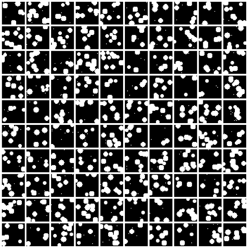
(b) 2D representation

Figure 2: Example 1: Training microstructure. Spherical inclusions embedded in a matrix material as used throughout Section 4. (a) Three-dimensional representation of a single microstructure with suppressed matrix. (b) Center plane slices of $1\times 10^{2}$ three-dimensional microstructures.

4.1 Filter topology for the discriminator: constant versus growing

First, two topology variants for the discriminator $\mathcal{D}$ from Eq. (7) are investigated with respect to their performance in the evaluation metrics from Section 3.7 as well as the number of parameters $\bm{\theta}$ from Eq. (4). The generator topology described in Section 3.1 is fixed for both discriminator topologies and works with a decreasing number of filters to map the low dimensional random input vector $\bm{z}$ to the image dimension, as shown in Figure 1. Here, the number of filters of the last transpose convolutional block is kept at $n_{f}^{\mathcal{G}}=32$.

Concerning the discriminator, the number of filters can be distributed in the same manner as for the generator, i.e. growing or evenly distributed. While both variants were presented in the literature, e.g., [63] for growing and [39] for constant filters, it is not clear which variant leads to the best results. Therefore, in this experiment, the total number of parameters was fixed to lay within in the order of $\bm{\theta}_{\mathcal{D}}=3.5\times 10^{6}$ while distributing them either in a growing way or evenly. Using $n_{L}=5$ residual blocks as defined in Section 3.2 for both topologies, this results in $n_{f}^{\mathcal{D}}=16$ filters for the first layer of the growing topology and $n_{f}^{\mathcal{D}}=120$ filters for the constant topology. Both the generator and discriminator are trained for $n_{\text{iter}}=1\times 10^{5}$ iterations. The number of training samples was chosen as $1\times 10^{4}$. The resulting metrics for $n_{s}=1\times 10^{3}$ different samples can be seen in Table 2. As reported in [64], this number of samples is sufficient for the mean of the quantities of interest. The relative error, as defined in Eq. (34), of the 1-point probability function or inclusion volume fraction defined in Eq. (18) is $\mathcal{E}_{{p}_{1}}=4.660\times 10^{-2}$ for the growing discriminator topology and $\mathcal{E}_{{p}_{1}}=1.378\times 10^{-1}$ for the constant discriminator topology. The relative error of the 2-point probability function defined in Eq. (19) is $\mathcal{E}_{{p}_{2}}=2.786\times 10^{-2}$ for the growing discriminator topology and $\mathcal{E}_{{p}_{2}}=6.892\times 10^{-2}$ for the constant discriminator topology. The 2-point probability distributions of both topologies are illustrated in Figure 3. The relative error of the homogenized $\bar{\mathbb{C}}_{11}$ component as defined in Section 2.3 is $\mathcal{E}_{\bar{\mathbb{C}}_{11}}=7.266\times 10^{-3}$ for the growing discriminator topology and $\mathcal{E}_{\bar{\mathbb{C}}_{11}}=6.399\times 10^{-2}$ for the constant discriminator topology.

Besides leading to worse results, the constant filter topology takes with 3h significantly longer time to train, compared to the growing topology with 1h. The reason for this is the convolution operation with respect to the larger number of filters in the first convolutional block for the constant layout $n_{f}^{\mathcal{D}}=120$ versus the growing layout $n_{f}^{\mathcal{D}}=16$. In the first block, the spatial dimensions of the are high compared to the later blocks. Here, the convolution operation is significantly more expansive. For the rest of this paper, the growing topology is used for the discriminator and a decreasing topology for the generator, where for the latter the same reasoning applies.

Topology	$\mathcal{E}_{{p}_{1}}$	$\mathcal{E}_{{p}_{2}}$	$\mathcal{E}_{\bar{\mathbb{C}}_{11}}$
Growing	$4.660\times 10^{-2}$	$2.786\times 10^{-2}$	$7.266\times 10^{-3}$
Constant	$1.378\times 10^{-1}$	$6.892\times 10^{-2}$	$6.399\times 10^{-2}$

Table 2: Example 1: Deviation from a reference solution using different discriminator topologies as described in Section 4.1. Here, a topology with growing filter size is compared to a topology using constant filter size, where the total number of parameters $\bm{\theta}$ for both the generator and the discriminator is kept equal.

Figure 3: Example 1: Growing versus constant: Two-point correlation functions for the dataset and the discriminators with growing and constant filter size from Section 4.1. Here, a topology with growing filter size is compared to a topology using constant filter size, where the total number of parameters $\bm{\theta}$ for both the generator and the discriminator is kept equal.

4.2 Influence of filter number for the discriminator

This section deals with the influence of the number of filters $n_{f}^{\mathcal{D}}$ of the discriminator $\mathcal{D}$ on the ability to generate synthetic microstructures, measured with respect to the first component of the homogenized elasticity tensor, ${\bar{\mathbb{C}}_{11}}$. To this end, a fixed generator topology with $n_{f}^{\mathcal{G}}=32$ filters in the last transpose residual convolution block $\mathcal{N}_{\text{ResConvT}}$ from Eq. (24) is chosen and a total of $n_{L}^{\mathcal{G}}=5$ blocks is used. For the discriminator, the number of filters $n_{f}^{\mathcal{D}}=32$ in the first residual convolutional block $\mathcal{N}_{\text{ResConv}}$ from Eq. (28) are varied, such that $n_{f}^{\mathcal{D}}=[8,16,32,64]$, where the total number of weights $\bm{\theta}_{\mathcal{D}}$ grows exponentially. The number of convolutional blocks is $n_{L}^{\mathcal{D}}=5$ for all discriminators. For $n_{f}^{\mathcal{D}}=[8,16,32,64]$ and the given number of blocks, the number of weights for the discriminator are $\bm{\theta}_{\mathcal{D}}=[0.9,3.5,14.3,57]\times 10^{6}$, respectively. To investigate the effect of the number of training samples $n_{s}$ of the dataset $\mathbb{D}$ from Eq. (6) on the different discriminator topologies, all networks are trained on three different amounts of microstructural realizations, namely $n_{s}=[10^{2},10^{3},10^{4}]$. For all experiments, the discriminator and generator are trained for $n_{\text{iter}}=1\times 10^{6}$ steps each.

The resulting error of the first component of the elasticity tensor $\mathcal{E}_{\bar{\mathbb{C}}_{11}}$ is shown in Figure 4. A clear effect of both the number of filters as well as the number of training samples can be observed. For the smallest amount of training samples, $n_{s}=1\times 10^{2}$, the error increases for higher filter numbers until $n_{f}^{\mathcal{D}}=32$, where a plateau is reached. Using $n_{s}=1\times 10^{3}$ samples, a different behavior is observed. Here the error goes down for increasing filter numbers until $n_{f}^{\mathcal{D}}=32$, from where on the error rises. For the largest amount of training samples, $n_{s}=1\times 10^{4}$, the error goes down steadily, despite of the number of filters. This effect can be explained by an overfitting behavior of the discriminator, when the capacity, by means of the total number of weights $\bm{\theta}_{\mathcal{D}}$, is large with respect to the number of samples $n_{s}$. Then, the discriminator will always be able to distinguish between generated images and training samples and assign large Wasserstein distances to them, despite the quality of the synthetic images. This gives the generator poor gradient updates. The significance of this effect towards practical application is high. One has to take care of choosing the appropriate discriminator for the specific number of training samples at hand to avoid overfitting effects.

Figure 4: Example 1: Filter discriminator: Relative error of the homogenized elasticity tensor component $\bar{\mathbb{C}}_{11}$ with respect to the number of starting filters $n_{f}^{\mathcal{D}}$ of the discriminator and different number of samples $n_{s}$ from Section 4.2. The hyperparameters of the generator are fixed.

4.3 Influence of filter number for the generator

This section deals with the influence of the number of filters $n_{f}^{\mathcal{G}}$ of the generator $\mathcal{G}$ on the ability to generate synthetic microstructures, measured with respect to the first component of the homogenized elasticity tensor, ${\bar{\mathbb{C}}_{11}}$. To this end, a fixed discriminator topology with $n_{f}^{\mathcal{D}}=64$ filters in the first residual convolution block $\mathcal{N}_{\text{ResConv}}$ from Eq. (28) is chosen and a total of $n_{L}^{\mathcal{D}}=5$ blocks is used. This is the best performing topology from Section 4.2. For the generator the number of filters $n_{f}^{\mathcal{G}}=32$ in the last transpose residual convolutional block $\mathcal{N}_{\text{ResConvT}}$ from Eq. (24) are varied, such that $n_{f}^{\mathcal{G}}=[8,16,32,64]$, where the total number of weights $\bm{\theta}_{\mathcal{G}}$ grows exponentially. The number of transpose convolutional blocks is $n_{L}^{\mathcal{G}}=5$ for all generators. For $n_{f}^{\mathcal{G}}=[8,16,32,64]$ and the given number of blocks, the number of weights for the generator are $\bm{\theta}_{\mathcal{G}}=[0.3,0.6,1.6,5.5]\times 10^{6}$, respectively. The number of training samples $n_{s}$ of the dataset $\mathbb{D}$ from Eq. (6) is fixed at $n_{s}=10^{4}$ to prevent overfitting as observed in Section 4.2. For all experiments, the discriminator and generator are trained for $n_{\text{iter}}=1\times 10^{6}$ steps each.

The resulting error of the first component of the elasticity tensor $\mathcal{E}_{\bar{\mathbb{C}}_{11}}$ is shown in Figure 5. As no convergence for the largest topology, $n_{f}^{\mathcal{G}}=64$ could be observed, for that specific number of filters a re-run of the simulation for $n_{\text{iter}}=2\times 10^{6}$ steps was carried out. Besides slower convergence, a trend towards lower errors for larger generators, in the sense of parameters $\bm{\theta}_{\mathcal{G}}$ and filter size $n_{f}^{\mathcal{G}}$, can be observed. This indicates the usage of the largest possible generator topology available for the given computational power to achieve the lowest error.

Figure 5: Example 1: Filter generator: Relative error of the homogenized elasticity tensor component $\bar{\mathbb{C}}_{11}$ with respect to the number of starting filters $n_{f}^{\mathcal{G}}$ of the generator for $n_{\text{iter}}=10^{6}$ iterations from Section 4.3. The hyperparameters of the discriminator are fixed. The generator with $n_{f}=64$ filters did not converge within the maximum number of iterations. Therefore, an additional for $n_{\text{iter}}=2\times 10^{6}$ iterations was carried out and reported.

4.4 Influence of random input vector

Another interesting effect is observed at prediction time. To this end, in this section two random input vectors are distinguished explicitly, namely the training random input vector $\bm{z}_{\text{train}}$ and the prediction random input vector $\bm{z}_{\text{pred}}$. During training, the generator from Eq. (5) takes a normally distributed random vector $\bm{z}_{\text{train}}$ as input. Usually, the mean $\mu$ and standard deviation $\sigma$ from Eq. (20) are chosen as $\mu_{\text{train}}=0$ and $\sigma_{\text{train}}=1$, which results in the best training dynamics. Details can be found in standard texts such as [44] or [43]. In the experiments carried out in this section it was found that during prediction, the quality and variety of the generated microstructures strongly depends on the standard deviation $\sigma_{\text{pred}}$ of the random input $\bm{z}_{\text{pred}}$ and the discriminator capacity, in terms of parameters $\bm{\theta}_{\mathcal{D}}$, used during training. To illustrate this effect, we plot predictions of the same generator $\mathcal{G}$ from Eq. (5) trained with different discriminators $\mathcal{D}$ from Eq. (7) with varying standard deviations $\sigma_{\text{pred}}=[0.1,1.0,10.0]$ in $\bm{z}_{\text{pred}}$. Here, a generator with $n_{f}^{\mathcal{G}}=32$ filters was trained with discriminators using a filter size of $n_{f}^{\mathcal{D}}=[8,16,32,64]$. The remaining hyperparameters are chosen equally to that reported in Section 4.2. The resulting microstructures are shown in Figure 6.

It can be observed that the observed variety and quality of the generated images is lower for larger discriminators with a large number of filters $n_{f}^{\mathcal{D}}$ using a small standard deviation $\sigma_{\text{pred}}$. The larger the standard deviation is chosen, the higher the variety of the generated images. Furthermore, the largest discriminator with $n_{f}^{\mathcal{D}}=64$ shows significant disturbance in the images for small and medium standard deviations of $\sigma_{\text{pred}}=[0.1,1.0]$. For smaller discriminators, this effect weakens the smaller the number of filters gets. For the smallest discriminator with $n_{f}^{\mathcal{D}}=8$, for all investigated standard deviations, varying microstructures without defects could be generated. For the largest standard deviation, all networks produced high quality and diverse microstructures.

This effect is different from the well known truncation trick reported in [65], where a normal random input variable was replaced by a truncated normal random variable to reduce variance. Therein, the reduced variance led to higher image quality but smaller variation.

Concerning practical implications, care should be taken if large networks are used and only a small number of training samples is available. Then, a larger standard deviation than during training should be chosen during prediction time.

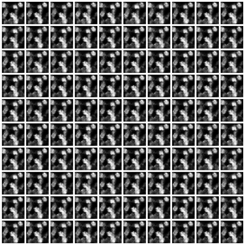
(a) $n_{f}^{\mathcal{D}}=64,\sigma_{\text{pred}}=0.1$

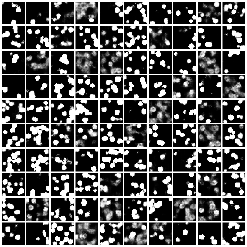
(b) $n_{f}^{\mathcal{D}}=64,\sigma_{\text{pred}}=1.0$

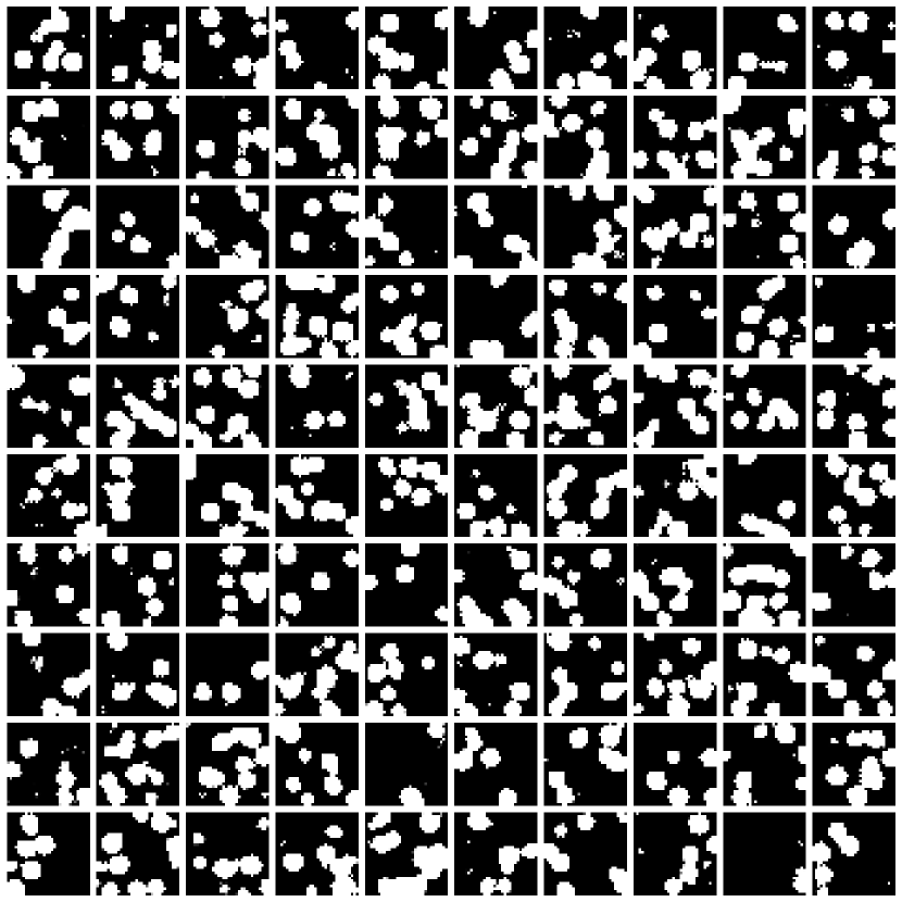
(c) $n_{f}^{\mathcal{D}}=64,\sigma_{\text{pred}}=10.0$

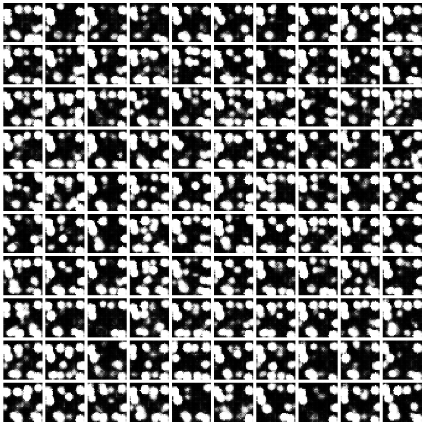
(d) $n_{f}^{\mathcal{D}}=32,\sigma_{\text{pred}}=0.1$

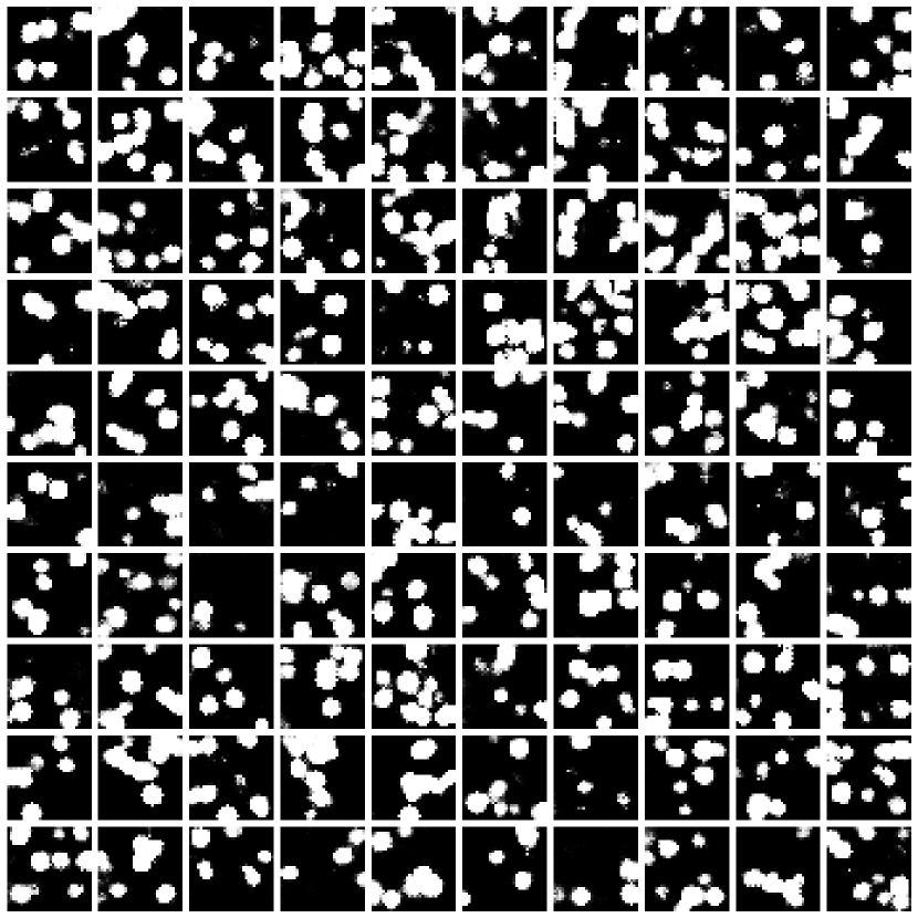
(e) $n_{f}^{\mathcal{D}}=32,\sigma_{\text{pred}}=1.0$

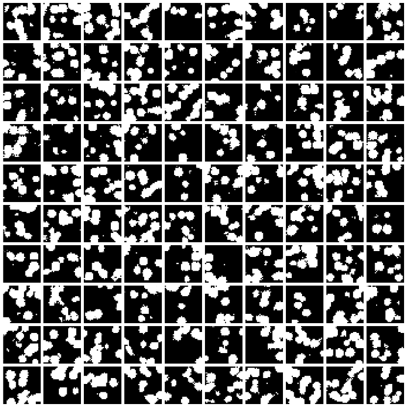
(f) $n_{f}^{\mathcal{D}}=32,\sigma_{\text{pred}}=10.0$

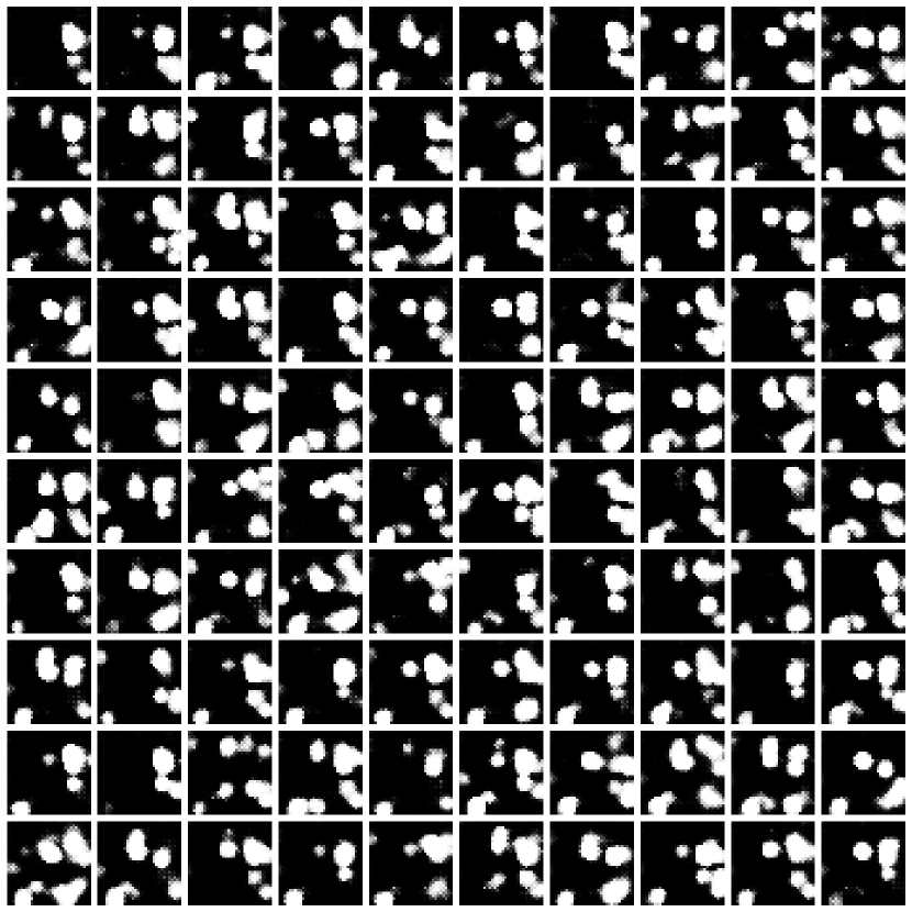
(g) $n_{f}^{\mathcal{D}}=16,\sigma_{\text{pred}}=0.1$

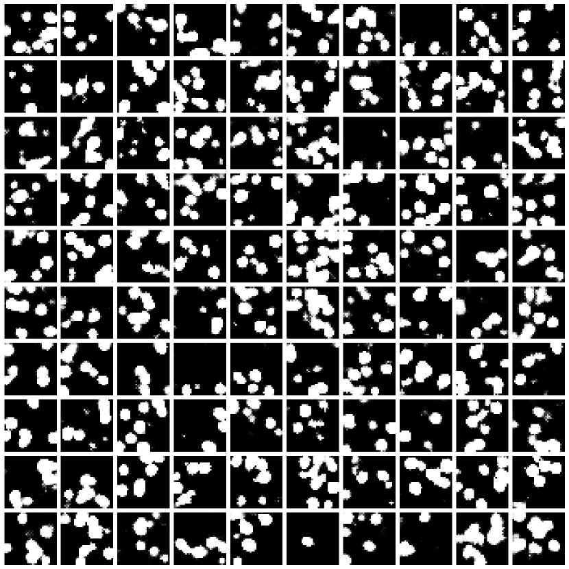
(h) $n_{f}^{\mathcal{D}}=16,\sigma_{\text{pred}}=1.0$

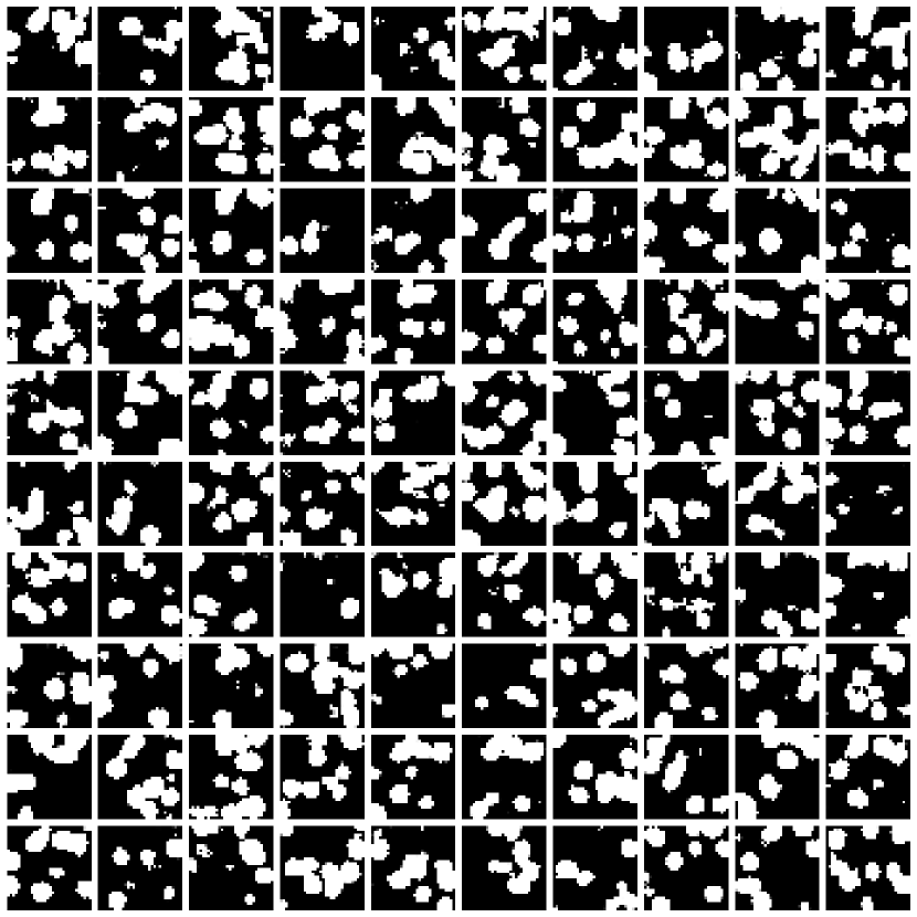
(i) $n_{f}^{\mathcal{D}}=16,\sigma_{\text{pred}}=10.0$

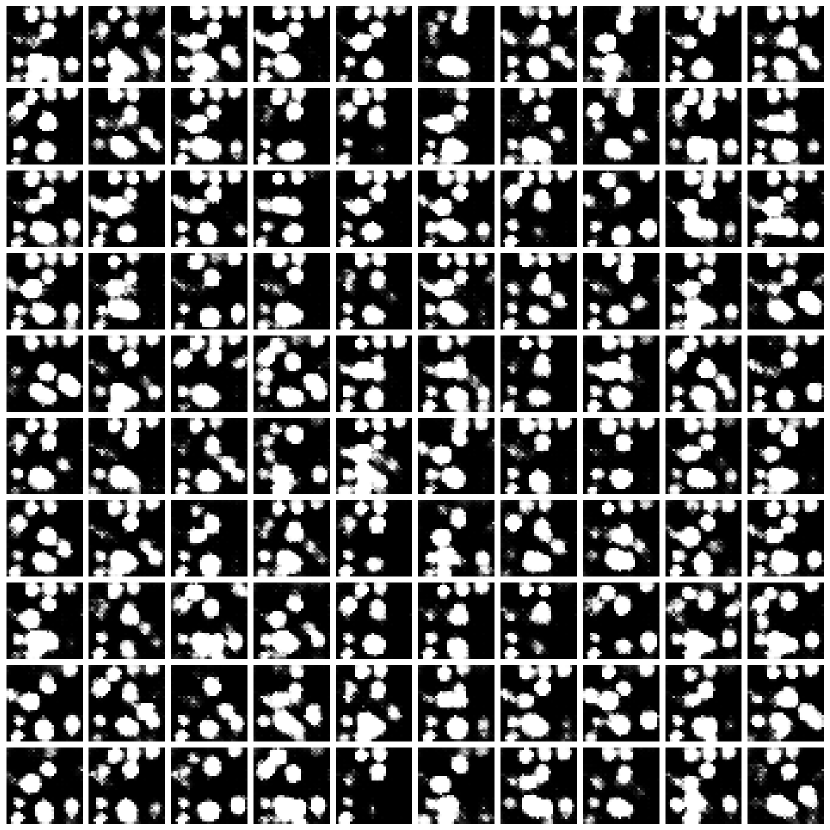
(j) $n_{f}^{\mathcal{D}}=8,\sigma_{\text{pred}}=0.1$

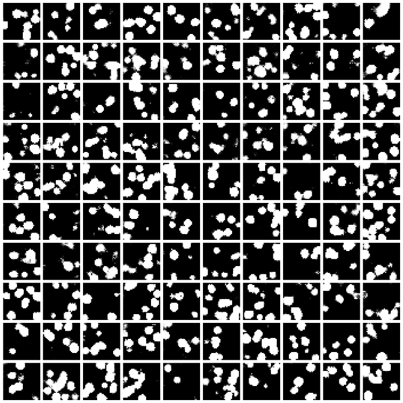
(k) $n_{f}^{\mathcal{D}}=8,\sigma_{\text{pred}}=1.0$

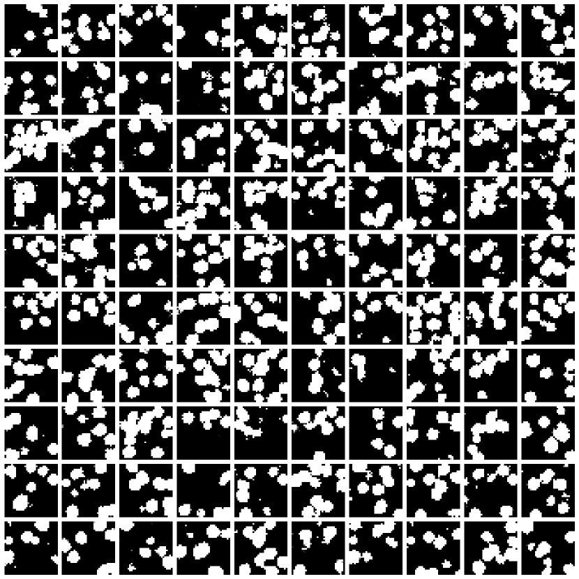
(l) $n_{f}^{\mathcal{D}}=8,\sigma_{\text{pred}}=10.0$

Figure 6: Example 1: Random input vector: Generated images of spherical inclusions from Section 4 for different discriminator filter sizes $n_{f}^{\mathcal{D}}$ used during training from Eq. (7). The generator is kept fixed with $n_{f}^{\mathcal{G}}=32$. Varying standard deviations of the random input vector $\bm{z}_{\text{pred}}$ from Eq. (20) are chosen. (a) $\sigma_{\text{pred}}=0.1$, (b) $\sigma_{\text{pred}}=1.0$, (c) $\sigma_{\text{pred}}=10.0$. Details can be found in Section 4.4

4.5 Best model

Finally, the best choice for the discriminator and generator were chosen as described in Section 4.2 and Section 4.3, respectively. The GAN was trained for $n_{\text{iter}}=2\times 10^{6}$ steps on $n_{s}=1\times 10^{4}$ training samples. The resulting metrics for $n_{s}=1\times 10^{3}$ different samples can be seen in Table 3, Figure 7 and Figure 8. The relative error of the 1-point probability function as defined in Eq. (34), which is identical to the inclusion volume fraction defined in Eq. (18), is $\mathcal{E}_{{p}_{1}}=3.464\times 10^{-2}$. The relative error of the 2-point probability function defined in Eq. (19) is $\mathcal{E}_{{p}_{2}}=2.438\times 10^{-2}$. The 2-point probability distribution is illustrated in Figure 7. The relative error of the homogenized $\bar{\mathbb{C}}_{11}$ component as defined in Section 2.3 is $\mathcal{E}_{\bar{\mathbb{C}}_{11}}=3.907\times 10^{-3}$. As can be seen in Table 3, the error with respect to the homogenized $\bar{\mathbb{C}}_{11}$ component is one magnitude lower than the errors in the n-point correlation functions and way below $1\%$ relative error. This shows, that the microstructural descriptors are not the primary drivers for the homogenized properties of the material. In this sense, the proposed GAN offers an advantage over descriptor driven generative approaches, as these do not enter explicitly in the optimization formulation. Moreover, the GAN learns the optimal descriptors during training only through the Wasserstein loss.

The results indicate, that the proposed GAN is able to generate highly accurate synthetic microstructures in the sense of micromechanical homogenized properties with respect to a training dataset.

$\mathcal{E}_{{p}_{1}}$	$\mathcal{E}_{{p}_{2}}$	$\mathcal{E}_{\bar{\mathbb{C}}_{11}}$
$3.463\times 10^{-2}$	$2.438\times 10^{-2}$	$3.907\times 10^{-3}$

Table 3: Example 1: Best model: Error measures for a generator with $n_{f}^{\mathcal{G}}=64$ filters trained by a discriminator with $n_{f}^{\mathcal{D}}=64$ filters for the best models as explained in Section 4.5.

Figure 7: Example 1: Best model. Two-point correlation functions for the dataset and a generator with $n_{f}^{\mathcal{G}}=64$ filters trained by a discriminator with $n_{f}^{\mathcal{D}}=64$ filters as described in Section 4.5.

(a) Real

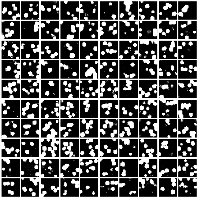
(b) Synthetic

Figure 8: Example 1: Best model. Spherical inclusions embedded in a matrix material. Center plane slices of $1\times 10^{2}$ three-dimensional microstructures. (a) Original data. (b) Synthetic microstructures generated by a generator with $n_{f}^{\mathcal{G}}=64$ filters trained by a discriminator with $n_{f}^{\mathcal{D}}=64$ filters. The standard deviation for $\bm{z}_{\text{pred}}$ was chosen as $\sigma_{\text{pred}}=10$. Details can be found in Section 4.5.

5 Example 2: Micro CT scan

For the second numerical experiment, a GAN is used to generate synthetic microstructures of a real-world $\mu$CT-scan of a wood-plastic composite (WPC). A filtered, binary micrograph with dimensions $950\times 240\times 850$ voxel, which is a total of $193.8\times 10^{6}$ voxels, is sliced into $1\times 10^{3}$ sub-volumes with dimensions $64\times 64\times 64$ via Latin-Hypercube sampling [66]. Every sub-volume has therefore $2.6\times 10^{5}$ voxels. The same material parameters for the matrix and inclusion as in Section 4 were chosen. The original $\mu$CT is illustrated in Figure 9.

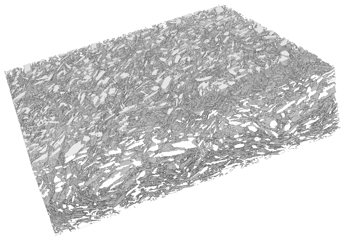
Figure 9: Micrograph of WPC as used in Section 5.

Because the image size is larger then the microstructures used in Section 4, an additional block has been included for both the generator and the discriminator, resulting in $n_{L}^{\mathcal{G}}=6$ and $n_{L}^{\mathcal{D}}=6$. For the generator, $n_{f}^{\mathcal{G}}=64$ filters in the last layer have been chosen, which results in a total of $\bm{\theta}_{\mathcal{G}}=21\times 10^{6}$ trainable weights. Given the number of training samples, for the discriminator, $n_{f}^{\mathcal{D}}=8$ filters in the first layer have been chosen, which results in a total of $\bm{\theta}_{\mathcal{D}}=3.6\times 10^{6}$ trainable weights. The training was carried out for $n_{\text{iter}}=3\times 10^{6}$ steps.

The resulting metrics for $n_{s}=1\times 10^{3}$ different samples can be seen in Table 4. The relative error as defined in Eq. (34) of the 1-point probability function or inclusion volume fraction defined in Eq. (18) is $\mathcal{E}_{{p}_{1}}=1.018\times 10^{-2}$. The relative error of the 2-point probability function defined in Eq. (19) is $\mathcal{E}_{{p}_{2}}=7.492\times 10^{-2}$. The 2-point probability distribution of both the original $\mu$CT-scan and the generator are illustrated in Figure 10. The relative error of the homogenized $\bar{\mathbb{C}}_{11}$ component as defined in Section 2.3 is $\mathcal{E}_{\bar{\mathbb{C}}_{11}}=7.348\times 10^{-3}$. Mid-plane sections of $1\times 10^{2}$ realizations of both the sub-volumes as well as the synthetic three-dimensional images are depicted in Figure 11.

It can be seen from the resulting error measures as well as from the generated images, that the proposed GAN is able to produce high quality synthetic microstructures on the basis of real-world $\mu$CT scans. It has to be pointed out, that only a single micrograph was used to train the GAN.

$\mathcal{E}_{{p}_{1}}$	$\mathcal{E}_{{p}_{2}}$	$\mathcal{E}_{\bar{\mathbb{C}}_{11}}$
$3.633\times 10^{-2}$	$5.121\times 10^{-2}$	$3.188\times 10^{-2}$

Table 4: Example 2: WPC: Error measures for a generator trained on a real $\mu$CT-Scan from Section 5.

Figure 10: Example 2: WPC: Two-point correlation functions for the WPC and the discriminator as described in Section 5.

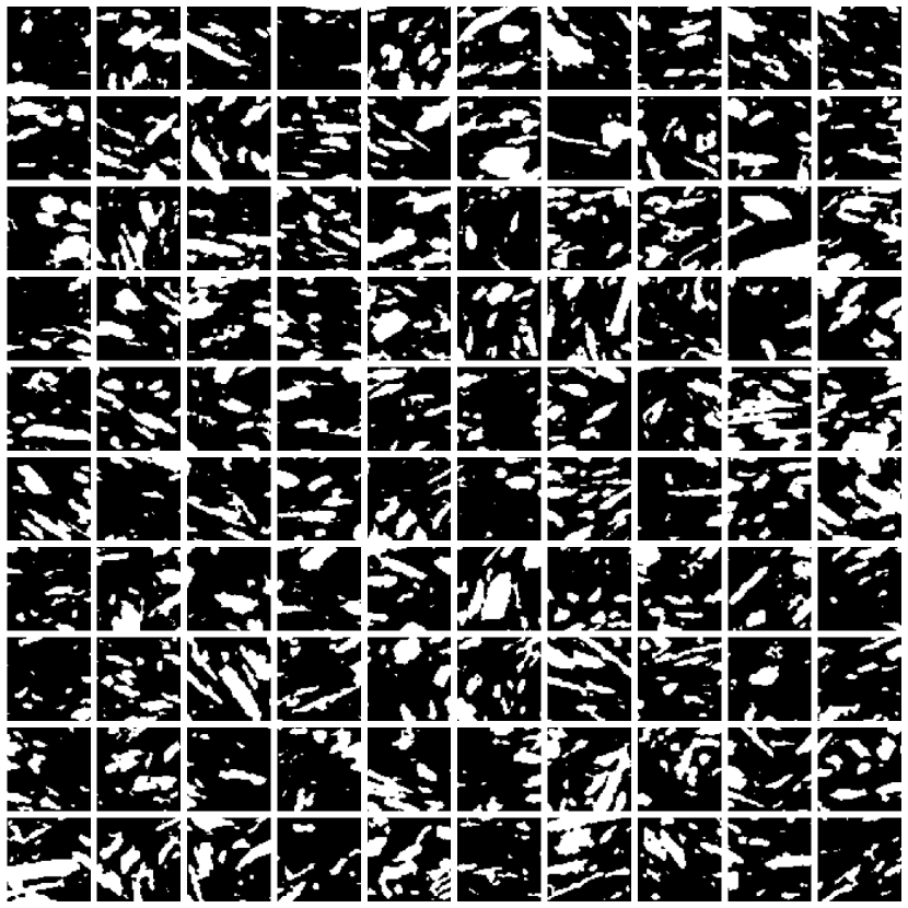
(a) Real

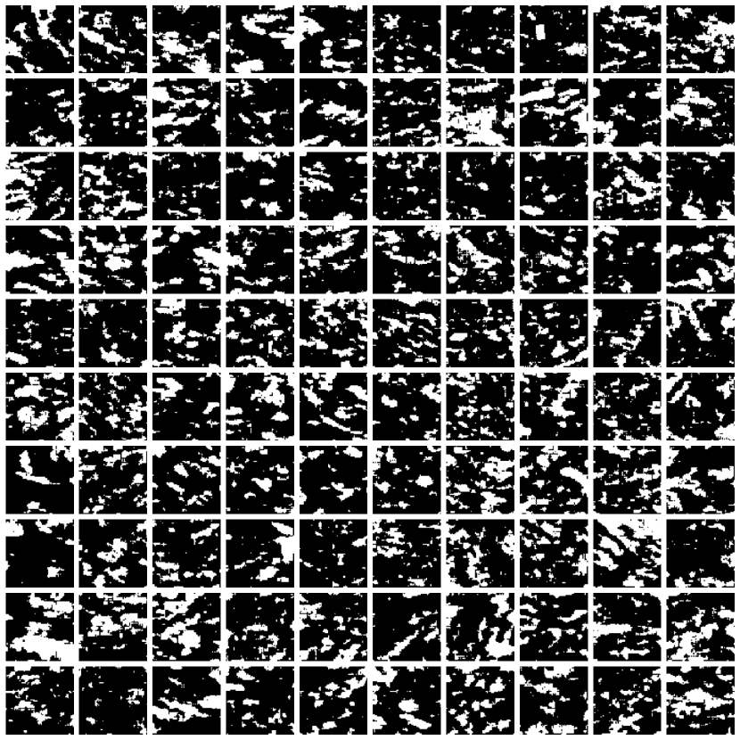
(b) Synthetic

Figure 11: Example 2: Training microstructure. Short wood fiber inclusions embedded in a polymer matrix material. Center plane slices of $1\times 10^{2}$ three-dimensional microstructures. (a) Original data. (b) Synthetic microstructures generated by a GAN from Section 5.

6 Conclusion and outlook

In the present study, a GAN for three-dimensional microstructure generation was proposed based on a convolutional-residual discriminator and a convolutional-residual generator with a nonlinear mapping network using a Wasserstein loss. Several numerical examples on different microstructures investigated the influence of hyperparameters on the synthesis quality with respect to evaluation metrics, such as n-point correlation functions and homogenized elasticity tensor components.

More specifically, the influence of the network topology was considered. A growing discriminator topology as well as a constant topology was compared, each with the same number of parameters. Both choices are present in the literature. It was shown, that the constant topology not only was more time consuming to train, but also suffered from slower convergence. Therefore, the growing topology was used throughout the rest of the paper for both the generator and discriminator.

Next, the influence of the number of filters of the discriminator with respect to the evaluation metrics was investigated. It was shown, that more filters lead to lower errors, if a large number of training samples are present. For smaller numbers of training samples, an overfitting behavior was recognized, which led to rising errors. This is an important finding due to its profound effects on practical considerations and has not yet been reported in the related literature. Generally, only a couple of hundreds of microstructures can be sliced from a handful of $\mu$CT-scans. Therefore, the capacity of the discriminator has to be balanced out with regard to the number of training samples. The effect of augmentation was not investigated, as in the specific use case presented in this work, the actual orientation of the microstructure is important due to its physical response with respect to defined loading directions. If the training microstructures are, e.g., rotated during augmentation, it is difficult to keep track of these manipulation.

Similar experiments were carried out for the generator, where the error went down for larger filter numbers, at the price of slower convergence. The general recommendation would be to use the largest generator possible having the hardware and project time schedule in mind.

An interesting effect with practical implications was observed at training time. Here, larger networks showed the tendency to produce microstructures with low variance and artifacts, if a random input vector with small standard deviation was used. For smaller networks, this effect was reduced. Using larger standard deviations in the input vector led to high quality, highly diverse microstructures with the desired properties.

The last experiments dealt with a real-world WPC micrograph. From this single micrograph, several sub-volumes were extracted. Given the limited amount of training samples, a small discriminator was chosen. The resulting high quality synthetic microstructures in combination with low error metrics underlined the generative capability of the proposed GAN, which is smaller in the sense of overall parameters as other state of the art generative networks proposed in the literature. This enables practitioners to train the network on a single workstation. It has to be pointed out, that the algorithm presented is able to extract information from a small number of $\mu$CT-scans to create artificial microstructures. Consequently, these microstructures only resemble the morphology of the training sample. Effects, which lie outside the considered training sample, cannot be captured. Here, more training data is needed.

Geometrical and physical inductive biases were considered but their practical use was declined. For a brief discussion about this, see the appendices.

Future communication will deal with the comparison with the wide range of other techniques of microstructure generation. Especially, a well established research area is the generation of microstructures using stochastic methods, e.g., [17] [18], [19], [20], [21]. Furthermore, the framework will be tested against more microstructural descriptors, especially the full elasticity tensor. Additionally, different materials, including more diverse morphologies of the underlying microstructure, such as concrete with pores, need to be explored. Some are currently under investigation by the authors.

The potential of this technology in engineering applications is high. To train e.g., a CNN for microstructure defect recognition or carrying out full field homogenization, such as in [11], a large number of training microstructures is needed. The number of costly $\mu$CT-scans can be significantly reduced, as the proposed GAN is able to efficiently amplify small datasets. The present work therefore closes a gap towards an end-to-end ANN driven homogenization framework, which is capable of predicting effective material properties from the microscale, trained on a small number of $\mu$CT-scans. Applications of these highly efficient approaches are real-time material property monitoring, i.e., structural health supervision, and multiscale simulations.

Appendix A S4-equivariant CNNs

In the literature, geometrical constraints to ANNs, exploiting equivariance to certain group operations such as translation and rotation, were introduced. The idea stem from the fact, that the convolution and cross-correlation operation in standard CNN are translational equivariant. Therefore, it is natural to think of different symmetry group operations, which aim to improve the accuracy and the training process. General equivariant ANNs, especially, group-equivariant convolutional neural networks (G-CNN), were first introduced for in [67]. Several works in two dimensions [68, 69, 70, 71] and in three dimensions [72, 73, 74, 75] followed. The idea was adapted to equivariant GANs for two-dimensional images in [31, 76] and for three-dimensional brain image data in [77]. In these works it was argued by the authors, that G-CNNs can reduce the amount of training images needed to avoid overfitting.

The ordinary convolutional neural network (CNN) using $\bm{h}_{\star}^{(l)}$ from Eq. (3) is translational equivariant. This enables the ANN to learn features of the image in different locations in the image, as opposed to the case of dense networks consisting only of dense layers $\bm{h}_{\cdot}^{(l)}$ from Eq. (3), which has to learn every feature for every location in the image. To further include rotational equivariance, in this work a S4-equivariant CNN was investigated, following [72]. S4 is the symmetry group of all $90\degree$ rotations of a cube. It is an expansion of the ordinary convolutional layer, where for each weight matrix $\bm{W}$ a rotated copy is created. This rotation can be achieved by the group action of S4, namely permutation of the entries of $\bm{W}$ by a precomputed index matrix. Then, the rotated filters are shifted or convoluted over the previous layer, such that

$$\bm{h}_{\text{S4}}^{(l)}=\left\{h_{\text{S4},\eta}^{(l)},\;\eta=1,\ldots,n_{u}\right\},\qquad h_{\text{S4},\eta}^{(l)}=\varphi^{(l)}\circ\;\phi^{(l)}\left(\mathbb{P}(\bm{W}^{(l)}_{\eta})\star\bm{h}^{(l-1)}\right),$$ ((35))

where $\mathbb{P}$ is a permutation matrix. Details can be found in [72]. In this work, the S4-convolutional layer was implemented as a custom TensorFlow 2 Keras layer to make use of GPU acceleration and parallelization.

Whereas the resulting microstructures are qualitatively good, the utilization of the S4 equivariant network was very challenging from a computational point of view, as for every learned filter a number of rotated copies has to be generated and stored. For practical applications, this becomes almost infeasible, as the wall time between the network presented in this work versus the S4 network is in the order of several hours to days versus several days to weeks, using a single workstation. For every unique filter, 24 copies have to be stored. Therefore, due to the large number of filters needed, the growing filter architecture is infeasible, such that the less performant constant layout has to be chosen.

Nevertheless, it is shown, that constant filter S4 discriminators provide good results. For the spherical inclusions investigated in Section 4, a standard generator with $n_{f}^{\mathcal{G}}=32$ filters was chosen. The discriminator utilized the equivariant layers from Eq. (35). Both networks used $n_{L}=5$ blocks. Both networks were trained for $n_{\text{iter}}=1\times 10^{5}$ iterations on $n_{s}=1\times 10^{3}$ training samples. Even after this relatively small number of iterations, the error of the $\bar{\mathbb{C}}_{11}$ component of the elasticity tensor with respect to $10^{3}$ different reference samples was $\mathcal{E}_{\bar{\mathbb{C}}_{11}}=1.5873\times 10^{-2}$. This is a good result and the generated microstructures are of high quality as illustrated in Figure 12. Nevertheless, the training was carried out for over one week, which makes it currently infeasible for practical applications, even more so due to memory limitations of current GPUs. In the future, scientist and engineers could profit from the enhanced convergence behavior of the S4 network.

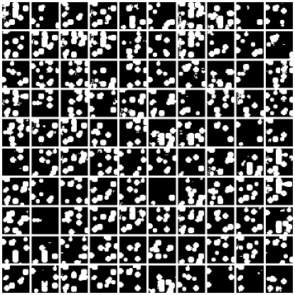
Figure 12: Center plane slices of $1\times 10^{2}$ 3D RVEs. Prediction by S4 network from Eq. (35).

Appendix B Physics informed GANs

As it was shown in [57] and [78], physical constraints can be introduced to ANN in the context of continuum mechanics, which enable the network to solve the underlying partial differential equations directly, without the need of training data. This approach is commonly known as physics informed neural networks. The introduction of explicit physics into the loss function was investigated, e.g., in [37]. Here, the standard GAN loss as introduced in [22] was used instead of the Wasserstein loss.

In this work, we also experimented with introducing a physical loss $\mathcal{L}_{p_{1}}$, taking into account the discrepancy of the inclusion fraction between the dataset and the generated images. Using the 1-point correlation function $p_{1}$ from Eq. (18), $\mathcal{L}_{p_{1}}$ is defined as

$$\mathcal{L}_{p_{1}}=\mathbb{E}\left[||p_{1}(\mathcal{I}_{\text{data}})-p_{1}(\mathcal{I}_{\text{synthetic}})||_{2}^{2}\right].$$ ((36))

No enhancement of the quality of the solution or the convergence behavior could be observed. Of course, more complex physical constraints could be introduced, e.g., Minkowski functionals or Minkowski tensors [79], but it is difficult to calculate these during training time due to computational burdens. In the light of the comment [80], the attempt to guide the optimization of the network by inductive bias is ultimately hopeless, as the universal approximation capacity of the neural network and the very general nature of the Wasserstein loss are sufficient, given enough computational power, to capture all properties of the microstructure at hand. This is one key advantage of the proposed GAN for microstructure generation, as no handcrafted descriptors of the microstructures enter the optimization process and therefore reduce human bias. Additionally, this enables the proposed GAN to be applicable to all possible kinds of materials, whereas descriptors, e.g., Minkowski functionals in the case of porous materials, are often tailored towards one specific material class.

Data availability

The code is available on https://github.com/ahenkes1/HENKES_GAN and [81].

References

- [1] J. Aboudi, S. M. Arnold, B. A. Bednarcyk, Micromechanics of composite materials: a generalized multiscale analysis approach, Butterworth-Heinemann, 2012.
- [2] H. J. Böhm, A short introduction to continuum micromechanics, in: Mechanics of microstructured materials, Springer, 2004, pp. 1–40.
- [3] S. Li, G. Wang, Introduction to micromechanics and nanomechanics, World Scientific Publishing Company, 2008.
- [4] S. Kumar, D. M. Kochmann, What machine learning can do for computational solid mechanics, in: Current Trends and Open Problems in Computational Mechanics, 2021.
- [5] K. Hornik, M. Stinchcombe, H. White, Multilayer feedforward networks are universal approximators, Neural networks 2 (5) (1989) 359–366.
- [6] Z. Yang, Y. C. Yabansu, R. Al-Bahrani, W.-k. Liao, A. N. Choudhary, S. R. Kalidindi, A. Agrawal, Deep learning approaches for mining structure-property linkages in high contrast composites from simulation datasets, Computational Materials Science 151 (2018) 278–287.
- [7] A. Beniwal, R. Dadhich, A. Alankar, Deep learning based predictive modeling for structure-property linkages, Materialia 8 (2019) 100435.
- [8] S. Ye, B. Li, Q. Li, H.-P. Zhao, X.-Q. Feng, Deep neural network method for predicting the mechanical properties of composites, Applied Physics Letters 115 (16) (2019) 161901.
- [9] A. L. Frankel, R. E. Jones, C. Alleman, J. A. Templeton, Predicting the mechanical response of oligocrystals with deep learning, Computational Materials Science 169 (2019) 109099.
- [10] C. Rao, Y. Liu, Three-dimensional convolutional neural network (3d-cnn) for heterogeneous material homogenization, Computational Materials Science 184 (2020) 109850.
- [11] A. Henkes, I. Caylak, R. Mahnken, A deep learning driven pseudospectral PCE based FFT homogenization algorithm for complex microstructures, Computer Methods in Applied Mechanics and Engineering 385 (2021) 114070.
- [12] H. Wessels, C. Böhm, F. Aldakheel, M. Hüpgen, M. Haist, L. Lohaus, P. Wriggers, Computational homogenization using convolutional neural networks, in: Current Trends and Open Problems in Computational Mechanics, Springer, 2022, pp. 569–579.
- [13] P. Carrara, R. Kruse, D. P. Bentz, M. Lunardelli, T. Leusmann, P. A. Varady, L. De Lorenzis, Improved mesoscale segmentation of concrete from 3d x-ray images using contrast enhancers, Cement and Concrete Composites 93 (2018) 30–42.
- [14] S. Bargmann, B. Klusemann, J. Markmann, J. E. Schnabel, K. Schneider, C. Soyarslan, J. Wilmers, Generation of 3d representative volume elements for heterogeneous materials: A review, Progress in Materials Science 96 (2018) 322–384.
- [15] M. Vicente, J. Mínguez, D. C. González, The use of computed tomography to explore the microstructure of materials in civil engineering: from rocks to concrete, InTech, 2017.
- [16] Y. He, H. Yu, X. Liu, Z. Yang, W. Sun, Y. Wang, Q. Fu, Y. Zou, A. Mian, Deep learning based 3d segmentation: A survey, arXiv preprint arXiv:2103.05423 (2021).
- [17] H. Wang, A. Pietrasanta, D. Jeulin, F. Willot, M. Faessel, L. Sorbier, M. Moreaud, Modelling mesoporous alumina microstructure with 3d random models of platelets, Journal of Microscopy 260 (3) (2015) 287–301.
- [18] V. Bortolussi, B. Figliuzzi, F. Willot, M. Faessel, M. Jeandin, Morphological modeling of cold spray coatings, Image Analysis and Stereology 37 (2) (2018) 145–158.
- [19] F. Willot, D. Jeulin, Elastic and electrical behavior of some randommultiscale highly-contrasted composites, International Journal for Multiscale Computational Engineering 9 (3) (2011).
- [20] B. Abdallah, F. Willot, D. Jeulin, Morphological modelling of three-phase microstructures of anode layers using sem images, Journal of microscopy 263 (1) (2016) 51–63.
- [21] M. Neumann, B. Abdallah, L. Holzer, F. Willot, V. Schmidt, Stochastic 3d modeling of three-phase microstructures for predicting transport properties: a case study, Transport in Porous Media 128 (1) (2019) 179–200.
- [22] I. Goodfellow, J. Pouget-Abadie, M. Mirza, B. Xu, D. Warde-Farley, S. Ozair, A. Courville, Y. Bengio, Generative adversarial nets, Advances in neural information processing systems 27 (2014).
- [23] D. M. Kreps, Nash equilibrium, in: Game Theory, Springer, 1989, pp. 167–177.
- [24] C. Villani, Optimal transport: old and new, Vol. 338, Springer, 2009.
- [25] C. Villani, Topics in optimal transportation, Vol. 58, American Mathematical Soc., 2021.
- [26] M. Arjovsky, L. Bottou, Towards principled methods for training generative adversarial networks, arXiv preprint arXiv:1701.04862 (2017).
- [27] M. Arjovsky, S. Chintala, L. Bottou, Wasserstein generative adversarial networks, in: International conference on machine learning, PMLR, 2017, pp. 214–223.
- [28] I. Gulrajani, F. Ahmed, M. Arjovsky, V. Dumoulin, A. Courville, Improved training of wasserstein gans, arXiv preprint arXiv:1704.00028 (2017).
- [29] T. Karras, S. Laine, T. Aila, A style-based generator architecture for generative adversarial networks, in: Proceedings of the IEEE/CVF Conference on Computer Vision and Pattern Recognition, 2019, pp. 4401–4410.
- [30] T. Karras, S. Laine, M. Aittala, J. Hellsten, J. Lehtinen, T. Aila, Analyzing and improving the image quality of stylegan, in: Proceedings of the IEEE/CVF Conference on Computer Vision and Pattern Recognition, 2020, pp. 8110–8119.
- [31] T. Karras, M. Aittala, S. Laine, E. Härkönen, J. Hellsten, J. Lehtinen, T. Aila, Alias-free generative adversarial networks, Advances in Neural Information Processing Systems 34 (2021).
- [32] J. Gui, Z. Sun, Y. Wen, D. Tao, J. Ye, A review on generative adversarial networks: Algorithms, theory, and applications, IEEE Transactions on Knowledge and Data Engineering (2021).
- [33] F. Carminati, A. Gheata, G. Khattak, P. M. Lorenzo, S. Sharan, S. Vallecorsa, Three dimensional generative adversarial networks for fast simulation, in: Journal of Physics: Conference Series, Vol. 1085, IOP Publishing, 2018, p. 032016.
- [34] S. Hong, R. Marinescu, A. V. Dalca, A. K. Bonkhoff, M. Bretzner, N. S. Rost, P. Golland, 3d-stylegan: A style-based generative adversarial network for generative modeling of three-dimensional medical images, in: Deep Generative Models, and Data Augmentation, Labelling, and Imperfections, Springer, 2021, pp. 24–34.
- [35] D. Wiesner, T. Nečasová, D. Svoboda, On generative modeling of cell shape using 3d gans, in: International Conference on Image Analysis and Processing, Springer, 2019, pp. 672–682.
- [36] D. Fokina, E. Muravleva, G. Ovchinnikov, I. Oseledets, Microstructure synthesis using style-based generative adversarial networks, Physical Review E 101 (4) (2020) 043308.
- [37] R. Singh, V. Shah, B. Pokuri, S. Sarkar, B. Ganapathysubramanian, C. Hegde, Physics-aware deep generative models for creating synthetic microstructures, arXiv preprint arXiv:1811.09669 (2018).
- [38] J.-W. Lee, N. H. Goo, W. B. Park, M. Pyo, K.-S. Sohn, Virtual microstructure design for steels using generative adversarial networks, Engineering Reports 3 (1) (2021) e12274.
- [39] L. Mosser, O. Dubrule, M. J. Blunt, Reconstruction of three-dimensional porous media using generative adversarial neural networks, Physical Review E 96 (4) (2017) 043309.
- [40] T. Hsu, W. K. Epting, H. Kim, H. W. Abernathy, G. A. Hackett, A. D. Rollett, P. A. Salvador, E. A. Holm, Microstructure generation via generative adversarial network for heterogeneous, topologically complex 3d materials, JOM 73 (1) (2021) 90–102.
- [41] A. Gayon-Lombardo, L. Mosser, N. P. Brandon, S. J. Cooper, Pores for thought: generative adversarial networks for stochastic reconstruction of 3d multi-phase electrode microstructures with periodic boundaries, npj Computational Materials 6 (1) (2020) 1–11.
- [42] C. M. Bishop, Pattern recognition and machine learning, springer, 2006.
- [43] I. Goodfellow, Y. Bengio, A. Courville, Y. Bengio, Deep learning, Vol. 1, MIT press Cambridge, 2016.
- [44] C. C. Aggarwal, et al., Neural networks and deep learning, Springer 10 (2018) 978–3.
- [45] A. Géron, Hands-on machine learning with Scikit-Learn, Keras, and TensorFlow: Concepts, tools, and techniques to build intelligent systems, O’Reilly Media, 2019.
- [46] F. Chollet, et al., Deep learning with Python, Vol. 361, Manning New York, 2018.
- [47] M. B. Hauser, Principles of riemannian geometry in neural networks, PhD thesis (2018).
- [48] A. Kennington, Differential geometry reconstructed: a unified systematic framework, http://www.topology.org/tex/conc/dg.html (2022).
- [49] D. Xiu, Numerical methods for stochastic computations, in: Numerical Methods for Stochastic Computations, Princeton university press, 2010.
- [50] J. Vondřejc, J. Zeman, I. Marek, An fft-based galerkin method for homogenization of periodic media, Computers & Mathematics with Applications 68 (3) (2014) 156–173.
- [51] T. De Geus, J. Vondřejc, J. Zeman, R. Peerlings, M. Geers, Finite strain fft-based non-linear solvers made simple, Computer Methods in Applied Mechanics and Engineering 318 (2017) 412–430.
- [52] J. Zeman, T. W. de Geus, J. Vondřejc, R. H. Peerlings, M. G. Geers, A finite element perspective on nonlinear fft-based micromechanical simulations, International Journal for Numerical Methods in Engineering 111 (10) (2017) 903–926.
- [53] M. Schneider, A review of nonlinear fft-based computational homogenization methods, Acta Mechanica (2021) 1–50.
- [54] A. Clément, C. Soize, J. Yvonnet, Uncertainty quantification in computational stochastic multiscale analysis of nonlinear elastic materials, Computer Methods in Applied Mechanics and Engineering 254 (2013) 61–82.
- [55] A. L. Maas, A. Y. Hannun, A. Y. Ng, et al., Rectifier nonlinearities improve neural network acoustic models, in: Proc. icml, Vol. 30, Citeseer, 2013, p. 3.
- [56] M. D. Zeiler, D. Krishnan, G. W. Taylor, R. Fergus, Deconvolutional networks, in: 2010 IEEE Computer Society Conference on computer vision and pattern recognition, Springer Cham, 2022.
- [57] A. Henkes, H. Wessels, R. Mahnken, Physics informed neural networks for continuum micromechanics, Computer Methods in Applied Mechanics and Engineering 393 (2022) 114790.
-
[58]
M. Abadi, A. Agarwal, P. Barham, E. Brevdo, Z. Chen, C. Citro, G. S. Corrado,
A. Davis, J. Dean, M. Devin, S. Ghemawat, I. Goodfellow, A. Harp, G. Irving,
M. Isard, Y. Jia, R. Jozefowicz, L. Kaiser, M. Kudlur, J. Levenberg,
D. Mané, R. Monga, S. Moore, D. Murray, C. Olah, M. Schuster, J. Shlens,
B. Steiner, I. Sutskever, K. Talwar, P. Tucker, V. Vanhoucke, V. Vasudevan,
F. Viégas, O. Vinyals, P. Warden, M. Wattenberg, M. Wicke, Y. Yu,
X. Zheng, TensorFlow: Large-scale
machine learning on heterogeneous systems, software available from
tensorflow.org (2015).
URL https://www.tensorflow.org/ - [59] S. Markidis, S. W. Der Chien, E. Laure, I. B. Peng, J. S. Vetter, Nvidia tensor core programmability, performance & precision, in: 2018 IEEE international parallel and distributed processing symposium workshops (IPDPSW), IEEE, 2018, pp. 522–531.
- [60] T. Dozat, Incorporating nesterov momentum into adam (2016).
- [61] A. M. Saxe, J. L. McClelland, S. Ganguli, Exact solutions to the nonlinear dynamics of learning in deep linear neural networks, arXiv preprint arXiv:1312.6120 (2013).
-
[62]
J. T. Gostick, Z. A. Khan, T. G. Tranter, M. D. Kok, M. Agnaou, M. Sadeghi,
R. Jervis, Porespy: A python
toolkit for quantitative analysis of porous media images, Journal of Open
Source Software 4 (37) (2019) 1296.
doi:10.21105/joss.01296.
URL https://doi.org/10.21105/joss.01296 - [63] H. Li, Y. Zheng, X. Wu, Q. Cai, 3d model generation and reconstruction using conditional generative adversarial network, International Journal of Computational Intelligence Systems 12 (2) (2019) 697.
- [64] B. Sudret, S. Marelli, J. Wiart, Surrogate models for uncertainty quantification: An overview, in: 2017 11th European conference on antennas and propagation (EUCAP), IEEE, 2017, pp. 793–797.
- [65] M. Marchesi, Megapixel size image creation using generative adversarial networks, arXiv preprint arXiv:1706.00082 (2017).
- [66] M. D. McKay, R. J. Beckman, W. J. Conover, A comparison of three methods for selecting values of input variables in the analysis of output from a computer code, Technometrics 42 (1) (2000) 55–61.
- [67] T. Cohen, M. Welling, Group equivariant convolutional networks, in: International conference on machine learning, PMLR, 2016, pp. 2990–2999.
- [68] T. S. Cohen, M. Welling, Steerable cnns, arXiv preprint arXiv:1612.08498 (2016).
- [69] T. S. Cohen, M. Geiger, J. Köhler, M. Welling, Spherical cnns, arXiv preprint arXiv:1801.10130 (2018).
- [70] T. Cohen, M. Weiler, B. Kicanaoglu, M. Welling, Gauge equivariant convolutional networks and the icosahedral cnn, in: International Conference on Machine Learning, PMLR, 2019, pp. 1321–1330.
- [71] T. Cohen, et al., Equivariant convolutional networks, PhD thesis (2021).
- [72] D. Worrall, G. Brostow, Cubenet: Equivariance to 3d rotation and translation, in: Proceedings of the European Conference on Computer Vision (ECCV), 2018, pp. 567–584.
- [73] M. Weiler, M. Geiger, M. Welling, W. Boomsma, T. S. Cohen, 3d steerable cnns: Learning rotationally equivariant features in volumetric data, Advances in Neural Information Processing Systems 31 (2018).
- [74] M. Winkels, T. S. Cohen, 3d g-cnns for pulmonary nodule detection, arXiv preprint arXiv:1804.04656 (2018).
- [75] M. M. Bronstein, J. Bruna, T. Cohen, P. Veličković, Geometric deep learning: Grids, groups, graphs, geodesics, and gauges, arXiv preprint arXiv:2104.13478 (2021).
- [76] N. Dey, A. Chen, S. Ghafurian, Group equivariant generative adversarial networks, in: International Conference on Learning Representations, 2020.
- [77] N. Dey, M. Ren, A. V. Dalca, G. Gerig, Generative adversarial registration for improved conditional deformable templates, in: Proceedings of the IEEE/CVF International Conference on Computer Vision, 2021, pp. 3929–3941.
- [78] H. Wessels, C. Weißenfels, P. Wriggers, The neural particle method–an updated lagrangian physics informed neural network for computational fluid dynamics, Computer Methods in Applied Mechanics and Engineering 368 (2020) 113127.
- [79] F. Ernesti, M. Schneider, S. Winter, D. Hug, G. Last, T. Böhlke, Characterizing digital microstructures by the minkowski-based quadratic normal tensor, arXiv preprint arXiv:2007.15490 (2020).
-
[80]
R. Sutton, The
bitter lesson (2019).
URL http://www.incompleteideas.net/IncIdeas/BitterLesson.html - [81] A. Henkes, H. Wessels, Three-dimensional microstructure generation using generative adversarial neural networks in the context of continuum micromechanics (Jul 2022). doi:10.5281/zenodo.6924533.