Abstract

Inferring causal structures from experimentation is a central task in many domains. For example, in biology, recent advances allow us to obtain single-cell expression data under multiple interventions such as drugs or gene knockouts. However, the targets of the interventions are often uncertain or unknown and the number of observations limited. As a result, standard causal discovery methods can no longer be reliably used. To fill this gap, we propose a Bayesian framework (BaCaDI) for discovering and reasoning about the causal structure that underlies data generated under various unknown experimental or interventional conditions. BaCaDI is fully differentiable, which allows us to infer the complex joint posterior over the intervention targets and the causal structure via efficient gradient-based variational inference. In experiments on synthetic causal discovery tasks and simulated gene-expression data, BaCaDI outperforms related methods in identifying causal structures and intervention targets.

1 INTRODUCTION

Identifying causal dependencies via empirical observation and experimentation is a problem of fundamental scientific interest. If we understand the causal mechanisms that govern a system of interest, we can predict its behavior when parts of system are actively manipulated from outside. For instance, if we understand the causal structure of a gene regulatory network, we can predict the effect of drugs or gene knockouts more reliably (Meinshausen et al.,, 2016). While identifying the true causal structure from observational data is often impossible (Pearl,, 2009; Peters et al.,, 2017), intervening on variables in the system and observing the outcome can fully identify the true causal structure in the large sample limit and the absence of latent confounders (Eberhardt et al.,, 2005, 2006; Hyttinen et al.,, 2013).

Intervening in real-world systems, however, is often costly and imprecise, resulting in a limited number of observations and uncertain or unknown intervention targets and effects. For example, recent advances in biology enable the collection of single-cell gene expression data under various interventions such as chemical compounds or gene knockouts (Srivatsan et al.,, 2020; McFarland et al.,, 2020). Given this significant epistemic uncertainty, causal structure learning becomes a complex joint inference problem over the structure and the unknown intervention targets that ultimately allow its identification. However, existing causal discovery methods that leverage interventional data typically assume full knowledge of the targets or the statistical effect of the interventions (Hauser and Bühlmann,, 2012; Wang et al.,, 2017; Yang et al.,, 2018). Conversely, recent methods that are able to deal with imperfect or unknown interventions do not account for epistemic uncertainty during inference (Mooij et al.,, 2016; Ke et al.,, 2019; Brouillard et al.,, 2020; Squires et al.,, 2020). Thus, they frequently fail in realistic scenarios where interventional data is scarce.

Addressing these shortcomings, we introduce Bayesian Causal Discovery with unknown Interventions (BaCaDI), a fully Bayesian approach for inferring the complete joint posterior over the causal structure, the parameters of the causal mechanisms, and the interventions performed in each experimental context. Thus, BaCaDI provides a principled Bayesian approach for propagating the epistemic uncertainty across all latent quantities which would be infeasible when treating uncertainty quantification and intervention identification separately or sequentially. Moreover, BaCaDI operates in the continuous space of latent probabilistic representations of both causal Bayesian networks (CBNs) and interventions. This formulation allows us to approximate the complex joint posterior via efficient, gradient-based particle variational inference techniques, making our approach particularly scalable to causal systems of many variables.

In a range of experiments conducted on synthetic causal BNs and a realistic gene-expression simulator, BaCaDI significantly outperforms related methods in recovering the underlying causal structure and intervention targets. This holds even when the underlying model is strongly misspecifed as in the case of gene-expression data.

2 RELATED WORK

Continuous optimization for structure learning. Classical algorithms for causal structure learning typically rely on conditional independence tests (Spirtes et al.,, 2000; Solus et al.,, 2017) or combinatorial search (Chickering,, 2002; Huang et al.,, 2018). Initiated by Zheng et al., (2018), recent works reformulate structure learning as a continuous optimization problem (Zheng et al.,, 2020; Yu et al.,, 2019; Lachapelle et al.,, 2019; Brouillard et al.,, 2020), which allows using gradient-based learning algorithms for this task. Building on these techniques, a recent line of work considers performing Bayesian inference over the causal graph instead of learning a point estimate (Annadani et al.,, 2021; Lorch et al.,, 2021; Cundy et al.,, 2021). Our approach belongs to this category but is the first to consider Bayesian inference from multiple contexts with unknown interventions.

Causal discovery from multiple contexts. Learning a causal structure from datasets collected in different interventional contexts of the same causal system has been referred to as Joint Causal Inference (JCI) (Mooij et al.,, 2016). Multiple methods handle such combinations of observational and interventional data (Magliacane et al.,, 2016; Zhang et al.,, 2017; Hauser and Bühlmann,, 2012; Wang et al.,, 2017; Yang et al.,, 2018), but assume full knowledge of the interventions. Other methods build on the notion of invariance (Schölkopf et al.,, 2012; Peters et al.,, 2016; Meinshausen et al.,, 2016; Ghassami et al.,, 2017; Heinze-Deml et al.,, 2018; Huang et al.,, 2020), but either do not generalize to full graphs or make restrictive assumptions about the local causal effects.

Causal discovery with unknown interventions. Mooij et al., (2016), Squires et al., (2020) and Wang et al., (2022) make the unknown intervention setting amenable to standard causal discovery tools such as conditional independence and invariance tests. However, hypothesis tests typically require large datasets, making these methods brittle for realistic datasets of small size. Jaber et al., (2020) develop theoretical equivalence classes for a mixture of distributions with unknown interventions, focusing on the infinite sample setting.

Other recent works formulate continuous relaxations of the joint inference problem under unknown interventions and use gradient-based optimization to find the graph and targets (Ke et al.,, 2019; Brouillard et al.,, 2020; Faria et al.,, 2022). However, these methods only infer point estimates. We adopt a fully Bayesian approach that enables principled uncertainty quantification. Eaton and Murphy, (2007) is the only work doing the same, though only for discrete variables and using a dynamic programming approach that does not scale to large graphs.

3 BACKGROUND: CAUSAL DISCOVERY

Causal Bayesian Networks. A Bayesian network (BN) $({\bf{G}},{\bf{\Theta}})$ uses a directed acyclic graph (DAG) to model the joint density $p({\mathbf{x}})$ of $d$ variables ${\mathbf{x}}={x}_{1:d}$ via conditional probabilities. The joint distribution $p$ factorizes into a product of local conditional distributions $p_{i}({x}_{i}|{x}_{{\text{pa}_{{\bf{G}}}(i)}},{\bf{\Theta}})$ for each variable ${x}_{i}$, where ${\text{pa}_{{\bf{G}}}(i)}$ is the set of parents of node $i$ in ${\bf{G}}$ and the parameters ${\bf{\Theta}}$ describe the exact local conditional distributions. In a causal BN (CBN), the edges describe direct causal relations. For causal structure learning, we assume that there are no unmeasured confounding variables (causal sufficiency, cf. Pearl,, 2009; Spirtes et al.,, 2000; Peters et al.,, 2017).

Interventions. An intervention on the variable ${x}_{i}$ corresponds to replacing the conditional distribution $p_{i}$ by a new distribution $p_{i}^{I}$. An intervention is typically considered imperfect (soft) if the dependence on the causal parents remains and perfect (hard, structural) if all dependencies to the causal parents are removed, resulting in the mutilated graph ${\bf{G}}^{I_{k}}$ (e.g. Pearl,, 2009; Peters et al.,, 2017).

In this work, we assume the setting of a collection of $M$ interventions $\mathcal{I}:=(I_{1},\dots I_{M})$, where each intervention $I_{k}:=(I^{\text{tar}}_{k},{\bf{\Theta}}_{I_{k}})$ acts on a set of targets $I^{\text{tar}}_{k}\subseteq\{1,\dots,d\}$. We use ${\bf{\Theta}}_{I_{k}}$ to denote parameters that describe the individual conditional distributions $p_{i}^{I_{k}}({x}_{i}|{x}_{{\text{pa}_{{\bf{G}}}(i)}},{\bf{\Theta}}_{I_{k}})$ induced by the intervention $I_{k}$ on the target variables $\{x_{i}|~{}i\in I^{\text{tar}}_{k}\}$. To simplify our exposition, we assume perfect interventions, i.e., $p_{i}^{I_{k}}({x}_{i}|{x}_{{\text{pa}_{{\bf{G}}}(i)}},{\bf{\Theta}}_{I_{k}})=p_{i}^{I_{k}}({x}_{i}|{\bf{\Theta}}_{I_{k}})$. However, all the arguments made in this paper also hold for soft interventions. The full data distribution under intervention $I_{k}$ factorizes into the observational and interventional conditionals:

$$\begin{split}p({\mathbf{x}}|{\bf{\Theta}},{\bf{G}},I_{k})=\prod_{i\notin I_{k}}p_{i}({x}_{i}|{x}_{{\text{pa}_{{\bf{G}}}(i)}},{\bf{\Theta}})\cdot\prod_{i\in I_{k}}p_{i}^{I_{k}}({x}_{i}|{\bf{\Theta}}_{I_{k}})\end{split}$$

The local conditional distributions of the variables that are not intervened upon do not change with respect to the observational distribution, which is often referred to as invariance (Peters et al.,, 2016) or modularity (Peters et al.,, 2017).

Bayesian Inference of BNs. Given passively collected i.i.d. observations $\mathcal{D}=\{{\mathbf{x}}^{(1)},\dots,{\mathbf{x}}^{(N)}\}$, Bayesian inference over BNs aims to estimate the full posterior probability density over BNs that model the observations. Following Friedman and Koller, (2003), given a prior distribution over DAGs $p({\bf{G}})$ and a prior over BN parameters $p({\bf{\Theta}}|{\bf{G}})$, Bayes’ Theorem yields the posterior distribution

$$p({\bf{G}},{\bf{\Theta}}|\mathcal{D}) \propto p({\bf{G}})p({\bf{\Theta}}|{\bf{G}})p(\mathcal{D}|{\bf{G}},{\bf{\Theta}})$$ (1)

where $p(\mathcal{D}|{\bf{G}},{\bf{\Theta}})=\prod_{i=1}^{n}p({\mathbf{x}}^{(i)}|{\bf{G}},{\bf{\Theta}})$ is the likelihood of the independent observations in $\mathcal{D}$, here without interventions on the system. Given the posterior, the Bayesian formalism allows us to compute expectations of the form

$$\mathbb{E}_{p({\bf{G}},{\bf{\Theta}}|\mathcal{D})}\Big{[}f({\bf{G}},{\bf{\Theta}})\Big{]}$$ (2)

for any function $f$ of interest. For instance, to obtain the posterior predictive, we would use $f({\bf{G}},{\bf{\Theta}})=p({\mathbf{x}}|{\bf{G}},{\bf{\Theta}})$  (Madigan and Raftery,, 1994; Madigan et al.,, 1995). In active learning of CBNs, a commonly used $f$ is the expected information gain about ${\bf{G}}$ after certain interventions (Tong and Koller,, 2001; Murphy,, 2001; Cho et al.,, 2016; Agrawal et al.,, 2019). The posterior $p({\bf{G}},{\bf{\Theta}}|\mathcal{D})$ captures the epistemic uncertainty in the unknown graph and parameters. In the large sample limit, the weight of the prior vanishes and the posterior converges to the graphs and parameters that give the highest likelihood. Inferring the posterior is computationally challenging since there are super-exponentionally many, i.e., $\smash{\mathcal{O}(d!2^{\binom{d}{2}})}$, possible DAGs with $d$ nodes (Robinson,, 1973). Hence, computing the normalization constant $p(\mathcal{D})$ is generally intractable.

4 BAYESIAN CAUSAL DISCOVERY WITH MULTI-CONTEXT DATA

Problem Statement. In this section, we develop a general method for Bayesian inference of the CBN given multiple interventional datasets with unknown intervention targets and effects. Formally, we are given $M$ datasets $\mathbf{D}=\{\mathcal{D}_{1},...,\mathcal{D}_{M}\}$ that were generated under (unknown) interventions $\mathcal{I}=\{I_{1},\dots,I_{M}\}$. Each $\mathcal{D}_{k}$ is a set of i.i.d. samples $\mathcal{D}_{k}=\{{\mathbf{x}}^{(k,1)},\dots,{\mathbf{x}}^{(k,n_{k})}\}$ obtained from the interventional data distribution $p({\mathbf{x}}|{\bf{\Theta}},{\bf{G}},I_{k})$. Observational data, if available, can be added to $\mathbf{D}$ as $\mathcal{D}_{0}:=\mathcal{D}$ with intervention targets $I_{0}=\emptyset$.

Our goal is to infer the full, unknown CBN $({\bf{G}},{\bf{\Theta}})$ and the unknown interventions $\mathcal{I}$ given the datasets $\mathbf{D}$. The key difficulty compared to standard causal inference is that, in addition to the ground truth CBN, the intervention targets $I^{\text{tar}}_{k}$ and their data-generating parameters ${\bf{\Theta}}_{I_{k}}$ are unknown. Therefore, we effectively perform joint inference over $M$ mutilated graphs that are all connected through the unobserved graph ${\bf{G}}$.

Such inference is well-posed only if the structural changes implied by each intervention $I_{k}$ are sparse relative to the overall size of ${\bf{G}}$, i.e. $|I_{k}|\ll d$. If large parts of the causal model were intervened upon differently across contexts, there may be little or no overlap in the mutilated causal DAGs and thus few reasons for multitasking. This assumption has also been used in prior works (Brouillard et al.,, 2020) and is commonly referred to as the Sparse Mechanism Shift hypothesis (Schölkopf et al.,, 2021), which posits that distribution changes tend to manifest themselves in a sparse way.

Bayesian inference. In many relevant application domains such as biology, the observed samples $n_{k}$ are noisy and small in number. Hence, it is paramount to not only to predict a single prototype CBN alongside one intervention hypothesis per dataset but also to reason about their joint epistemic uncertainty. Such uncertainty estimates allow us to quantify the reliability of our predictions and can be used to actively design future experiments. We thus approach the problem from a Bayesian perspective. This renders the task of learning from $\mathbf{D}$ as a posterior inference problem, where the prior probability and likelihood function are chosen beforehand and serve as the antecedents of inference. We are going to gradually build up this problem in the following.

Known interventions. When the intervention targets $I^{\text{tar}}_{k}$ and the parameters ${\bf{\Theta}}_{I_{k}}$ of the intervention effect are known, for $k=1,\ldots,M$, the posterior over CBNs includes (i.) the product of data likelihoods over all datasets in $\mathbf{D}$, and (ii.) interventional instead of observation likelihoods for $\mathcal{D}_{k\geq 1}$ ,

$$\begin{split}p({\bf{G}},{\bf{\Theta}}|\mathbf{D},\mathcal{I})&\propto{}\underbrace{p({\bf{G}})p({\bf{\Theta}}|{\bf{G}})}_{\text{priors}}\underbrace{p(\mathcal{D}_{0}|{\bf{\Theta}},{\bf{G}})}_{\text{obs. likelihood}}\\ &~{}~{}~{}~{}\cdot\prod_{k=1}^{M}\underbrace{p(\mathcal{D}_{k}|{\bf{\Theta}},{\bf{G}},I_{k})}_{\text{interv. likelihood}}\;,\vspace{0pt}\end{split}$$ (3)

where $p(\mathcal{D}_{k}|{\bf{\Theta}},{\bf{G}},I_{k})=\prod_{i=1}^{n_{k}}p({\mathbf{x}}^{(k,i)}|{\bf{\Theta}},{\bf{G}},I_{k})$ is the interventional likelihood for $\mathcal{D}_{k}$ given $I_{k}=(I^{\text{tar}}_{k},{\bf{\Theta}}_{I_{k}})$.

Unknown interventions. We include unknown interventions in our inference model by introducing additional priors $p(I^{\text{tar}}_{k})$ and $p({\bf{\Theta}}_{I_{k}}|I^{\text{tar}}_{k})$. Accordingly, the modified posterior follows as

$$\begin{split}p({\bf{G}},{\bf{\Theta}},\mathcal{I}|&\mathbf{D})\propto{}\underbrace{p({\bf{G}})p({\bf{\Theta}}|{\bf{G}})}_{\text{priors}}\underbrace{p(\mathcal{D}_{0}|{\bf{\Theta}},{\bf{G}})}_{\text{obs. likelihood}}\\ &\cdot\prod_{k=1}^{M}\underbrace{p(I^{\text{tar}}_{k})p({\bf{\Theta}}_{I_{k}}|I^{\text{tar}}_{k})}_{\text{interv. priors}}\underbrace{p(\mathcal{D}_{k}|{\bf{\Theta}},{\bf{G}},I_{k})}_{\text{interv. likelihood}}\vspace{0pt}\end{split}$$ (4)

The prior $p(I^{\text{tar}}_{k})$ over intervention targets models prior beliefs about the structure of interventions, e.g., that only a sparse set of variables are subject to an intervention at the same time. The parameterization of the interventional distributions $p_{i}^{I}({x}_{i}|{\bf{\Theta}}_{I})$ is informed by the application and reflects the general nature of interventions, e.g., gene knockdowns in biology.

5 A DIFFERENTIABLE GENERATIVE MODEL OVER CBNs AND INTERVENTIONS

In the following, we represent ${\bf{G}}\in\{0,1\}^{d\times d}$ as the adjacency matrix and $I^{\text{tar}}_{k}=[I^{\text{tar}}_{k,1},...,I^{\text{tar}}_{k,d}]^{\top}\in\{0,1\}^{d}$ as the indicator vector where $I^{\text{tar}}_{k,l}=1$ if the $l$-th variable is intervened upon and $I^{\text{tar}}_{k,l}=0$ otherwise. Since multiple nodes may be intervened upon simultaneously, $I^{\text{tar}}_{k}$ is in general not one-hot. We write $\mathcal{I}^{\text{tar}}$ short for the stack $[I^{\text{tar}}_{1},...,I^{\text{tar}}_{M}]$ of intervention targets and ${\bf{\Theta}}_{\mathcal{I}}:=[{\bf{\Theta}}_{I_{1}},...,{\bf{\Theta}}_{I_{M}}]$ for the intervention effect parameters.

Challenges. The Bayesian inference task is intricate when learning from multiple datasets generated under interventions with unknown targets and effects. Learning the joint posterior in Eq. 4 requires working with a complex distribution over discrete DAGs ${\bf{G}}$, continuous mechanism parameters ${\bf{\Theta}}$, and interventions $\smash{\{I_{k}\}_{k=1}^{M}}$, which in turn affect the identification of the DAG ${\bf{G}}$ itself. Consequently, alternating inference of ${\bf{G}}$ and $\mathcal{I}^{\text{tar}}$ using an EM-like approach would preclude propagation of epistemic uncertainty across all latent quantities and thus lead to sub-optimal results.

Moreover, it is essential to infer the parameters of the interventional likelihoods $p_{i}^{I_{k}}({x}_{i}|{\bf{\Theta}}_{I_{k}})$ in Eq. 11 conditional upon predicting that an intervention occurred. This is of particular importance when interventions constitute a strong shift of distributions. By naively masking the observational likelihood when a variable is believed to be targeted, we would not evaluate the likelihood of the intervention itself and effectively operate outside the Bayesian framework. This would encourage the prediction of interventions whenever our learned model is suboptimal in explaining the data.

To tackle these joint inference challenges, we utilize ideas of Lorch et al., (2021), who introduce a method for efficient inference of the posterior of the CBN (${\bf{G}},{\bf{\Theta}}$) given a single observational dataset $\mathcal{D}$ by translating the distribution into a continuous latent space. Generalizing their approach, we transform our multi-context inference problem over the DAG ${\bf{G}}$ and the set of interventions targets $\{I^{\text{tar}}_{k}\}$ into one over only continuous latent variables that is consistent with the original task in Eq. 4 and that allows for the direct estimation of the score of the joint posterior over ${\bf{G}}$ and $I^{\text{tar}}_{k}$ in each context $k=1,\dots,M$. Devising such an inference scheme for the multi-context, unknown intervention setting requires careful modeling of the intervention target prior that accurately captures our assumptions of the data generating process, such as sparsity and sharpness of the interventions. At the same time, it must enable accurate and tractable inference via methods like variational inference (Blei et al.,, 2017) and perform well in practice.

To enable joint inference of all latent quantities, we introduce continuous latent variables ${\bf{Z}}$ and ${\bf{\Gamma}}_{k}$ and their corresponding priors, which model the generative processes of ${\bf{G}}$ and $I^{\text{tar}}_{k}$ through $p({\bf{G}}|{\bf{Z}})$ and $p(I^{\text{tar}}_{k}|{\bf{\Gamma}}_{k})$. This implies the following extended factorization of the generative model, which is also given in Figure 1:

Figure 1: Generative model of causal Bayesian networks with observations sampled in $M$ intervention contexts. The continuous variables $\{{\bf{\Gamma}}_{k}\}$ and ${\bf{Z}}$ extend the default data-generating process and allow reformulating the Bayesian inference task for gradient-based inference techniques.

$$p({\bf{Z}},{\bf{G}},{\bf{\Theta}},{\bf{\Gamma}},\mathcal{I},\mathbf{D})=\underbrace{p({\bf{Z}})p({\bf{G}}|{\bf{Z}})p({\bf{\Theta}}|{\bf{G}})}_{\text{generative process CBN}}$$ (5)

$$\cdot\prod_{k=1}^{M}\underbrace{p({\bf{\Gamma}}_{k})p(I^{\text{tar}}_{k}|{\bf{\Gamma}}_{k})p({\bf{\Theta}}_{I_{k}}|I^{\text{tar}}_{k})}_{\text{generative process intervention}}\underbrace{p(\mathcal{D}_{k}|{\bf{G}},{\bf{\Theta}},I^{\text{tar}}_{k},{\bf{\Theta}}_{I_{k}})}_{\text{interventional likelihood}}\vspace{-4pt}$$

where ${\bf{\Gamma}}:=[{\bf{\Gamma}}_{1},...,{\bf{\Gamma}}_{M}]$ for brevity. As shown in the following, the extended generative model we introduce allows expressing the posterior in Eq. 4 in terms of the posterior over the continuous latent variables ${\bf{Z}}$, ${\bf{\Theta}}$, ${\bf{\Gamma}}$, and ${\bf{\Theta}}_{\mathcal{I}}$:

Proposition 1

Under the extended generative model in Eq. 5 and Figure 1, it holds that

$$\mathbb{E}_{p({\bf{G}},{\bf{\Theta}},\mathcal{I}|\mathbf{D})}[f({\bf{G}},{\bf{\Theta}},\mathcal{I})]=$$ (6)

$$\mathbb{E}_{p({\bf{Z}},{\bf{\Theta}},{\bf{\Gamma}},{\bf{\Theta}}_{\mathcal{I}}|\mathbf{D})}\left[\frac{\mathbb{E}_{p({\bf{G}}|{\bf{Z}})}\mathbb{E}_{p(\mathcal{I}^{\text{tar}}|{\bf{\Gamma}})}[f({\bf{G}},{\bf{\Theta}},\mathcal{I})\cdot\mathbf{\Psi}]}{\mathbb{E}_{p({\bf{G}}|{\bf{Z}})}\mathbb{E}_{p(\mathcal{I}^{\text{tar}}|{\bf{\Gamma}})}[\mathbf{\Psi}]}\right]$$

with weighting $\mathbf{\Psi}=p({\bf{\Theta}}|{\bf{G}})p({\bf{\Theta}}_{\mathcal{I}}|\mathcal{I}^{\text{tar}})p(\mathbf{D}|{\bf{G}},\mathcal{I},{\bf{\Theta}})$ and $p(\mathbf{D}|{\bf{G}},\mathcal{I},{\bf{\Theta}})=\prod_{k=1}^{M}p(\mathcal{D}_{k}|{\bf{G}},{\bf{\Theta}},I^{\text{tar}}_{k},{\bf{\Theta}}_{I_{k}})$.

This insight shows that the posterior expectation over graphs and interventions can be computed via an expectation over the latent posterior $p({\bf{Z}},{\bf{\Theta}},{\bf{\Gamma}},{\bf{\Theta}}_{\mathcal{I}}|\mathbf{D})$. We provide a proof in Appx. A.1. The inner term is akin to a likelihood ratio of the considered $({\bf{G}},{\bf{\Theta}},\mathcal{I})$ under the posterior expectation over ${\bf{Z}}$ and ${\bf{\Gamma}}$. All factors besides the latent posterior are tractable to compute or approximate. Before we discuss how to perform approximate inference of $p({\bf{Z}},{\bf{\Theta}},{\bf{\Gamma}},{\bf{\Theta}}_{\mathcal{I}}|\mathbf{D})$, we further specify the conditional probabilities of our generative model and how to make them differentiable.

Generative model of DAGs ${\bf{G}}$. Following Lorch et al., (2021), we define the latent variable ${\bf{Z}}$ as the stack of embedding matrices $\mathbf{U},\mathbf{V}\in\mathbb{R}^{d\times d}$ and the generative model for the adjacency matrix ${\bf{G}}$ by using the inner product:

$$\begin{split}p_{\alpha}({\bf{G}}|{\bf{Z}})=&\prod_{i=1}^{d}\prod_{j\neq i}^{d}p_{\alpha}(g_{ij}|\mathbf{u}_{i},\mathbf{v}_{j})\\ ~{}~{}~{}\text{with}~{}~{}~{}&g_{ij}|\mathbf{u}_{i},\mathbf{v}_{j}\sim\text{Bern}(\sigma_{\alpha}(\mathbf{u}_{i}^{\top}\mathbf{v}_{j}))\vspace{0pt}\end{split}$$ (7)

where $\sigma_{\alpha}(x)=1/(1+\exp(-\alpha x))$ is the sigmoid function with inverse temperature $\alpha$ and $\mathbf{u}_{i}$, $\mathbf{v}_{j}$ the $i$-th and $j$-th column vectors of $\mathbf{U}$ and $\mathbf{V}$, respectively. The authors show that this formulation outperforms a scalar parametrization based on a $d\times d$ matrix. We denote the matrix of edge probabilities in ${\bf{G}}$ given ${\bf{Z}}$ by ${\bf{G}}_{\alpha}({\bf{Z}})\in[0,1]^{d\times d}$ with ${\bf{G}}_{\alpha}({\bf{Z}})_{ij}:=\sigma_{\alpha}(\mathbf{u}_{i}^{\top}\mathbf{v}_{j})$. We model the prior over ${\bf{Z}}$ as (i.) i.i.d. Gaussian with a variance of $\eta_{Z}^{2}=1/d$ to ensure well-behaved gradients and (ii.) an acyclicity term that penalizes the expected cyclicity of ${\bf{G}}$ given ${\bf{Z}}$ :

$$\begin{split}p_{\beta}(\mathbf{Z})=p(\mathbf{U},\mathbf{V})&\propto\underbrace{\exp\left(-\beta\mathbb{E}_{p({\bf{G}}|{\bf{Z}})}[h({\bf{G}})]\right)}_{\text{acyclicity prior}}\\ &\cdot\prod_{i=1}^{d}\underbrace{\mathcal{N}(\mathbf{u}_{i}|\bm{0},\eta_{Z}^{2}\mathbf{I})\mathcal{N}(\mathbf{v}_{i}|\bm{0},\eta_{Z}^{2}\mathbf{I})}_{\text{inference stability}}\;\vspace{0pt}\end{split}$$ (8)

Here, $\beta$ is an inverse temperature parameter controlling how strongly the acyclicity is enforced, and $h({\bf{G}})=\text{tr}\left[(I+\frac{1}{d}{\bf{G}})^{d}\right]-d\geq 0$. By Theorem 1 of Yu et al., (2019), ${\bf{G}}$ is acyclic iff $h(G)=0$. As $\beta\rightarrow\infty$, the support of $p(\mathbf{Z})$ reduces to all ${\bf{Z}}$ that model DAGs.

Generative model of intervention targets $\mathcal{I}^{\text{tar}}$. To model the intervention targets in continuous space, we introduce the latent variable ${\bf{\Gamma}}\in\mathbb{R}^{M\times d}$. Each $\gamma_{k,i}$ is the logit of an independent Bernoulli distribution and models one entry $(k,i)$ of the intervention target mask $\mathcal{I}^{\text{tar}}=[I^{\text{tar}}_{1},...,I^{\text{tar}}_{M}]\in\{0,1\}^{M\times d}$:

$$\begin{split}p(\mathcal{I}^{\text{tar}}|{\bf{\Gamma}})=&\prod_{k=1}^{M}\prod_{i=1}^{d}p_{\alpha}(I^{\text{tar}}_{k,i}|\gamma_{k,i})\\ ~{}~{}~{}\text{with}~{}~{}~{}&I^{\text{tar}}_{k,i}|\gamma_{k,i}\sim\text{Bern}(\sigma_{\alpha}(\gamma_{k,i}))\vspace{0pt}\end{split}$$ (9)

We denote the matrix of intervention target probabilities as $\mathcal{I}^{\text{tar}}_{\alpha}({\bf{\Gamma}})\in[0,1]^{M\times d}$ with $\mathcal{I}^{\text{tar}}_{\alpha}({\bf{\Gamma}})_{k,i}=\sigma_{\alpha}(\gamma_{k,i})$. The prior over ${\bf{\Gamma}}$ has three components: (i.) A Gaussian term for inference stability , (ii.) a Beta-distribution sharpness prior that encourages $\sigma_{\alpha}(\gamma_{k,i})$ to be close to 0 or 1, and (iii.) a sparsity prior with the $l_{1}$-norm of $\sigma_{\alpha}({\bf{\Gamma}}_{k})$ and the inverse temperature parameter $\lambda$.

$$\begin{split}p({\bf{\Gamma}})\propto&\prod_{k=1}^{M}\underbrace{\exp\left(-\lambda\lVert\sigma_{\alpha}({\bf{\Gamma}}_{k})\rVert_{1}\right)}_{\text{sparse masks}}\\ &\cdot\prod_{i=1}^{d}\underbrace{\text{Beta}(\sigma_{\alpha}(\gamma_{k,i});\zeta_{1},\zeta_{2})}_{\text{sharp masks}}\underbrace{\mathcal{N}(\gamma_{k}|\bm{0},\eta_{\gamma}^{2}\mathbf{I})}_{\text{inference stability}}\;\vspace{0pt}\end{split}$$ (10)

We assume that interventions occur infrequently, i.e., in expectation only on one variable. Hence, we choose $\zeta_{1}=1/d$ and $\zeta_{2}=(d-1)/d$. The sparsity prior implies that, given an active intervention target $i$, it is a-priori less likely that a variable $j\neq i$ is intervened upon in the same context $k$. The sparsity of interventions can additionally be regulated with the parameter $\lambda$.

Interventional likelihood. Combining the generative DAG and intervention models in Eqs. 8 and 9, we obtain a differentiable interventional likelihood by sampling the graph ${\bf{G}}\sim\text{Bern}\left(\smash{\sigma_{\alpha}(\mathbf{U}\mathbf{V}^{\top}})\right)$ and masks $\mathcal{I}^{\text{tar}}\sim\text{Bern}\left(\sigma_{\alpha}({\bf{\Gamma}})\right)$ with the Gumbel-Softmax trick (Jang et al.,, 2016; Maddison et al.,, 2017) and using them to select between the observational and interventional likelihoods for each variable:

$$p(\mathcal{D}_{k}|{\bf{G}},{\bf{\Theta}},I^{\text{tar}}_{k},{\bf{\Theta}}_{I_{k}})=$$ (11)

$$\prod_{j=1}^{n_{k}}\prod_{i=1}^{d}\left(p(x^{(k,j)}_{i}|{x}_{{\text{pa}_{{\bf{G}}}(i)}},{\bf{\Theta}})^{(1-I^{\text{tar}}_{k,i})}\cdot p(x^{(k,j)}_{i}|{\bf{\Theta}}_{I_{k}})^{I^{\text{tar}}_{k,i}}\right)\vspace{0pt}\vspace{-6pt}$$

Importantly, this formulation does not assume a specific likelihood or intervention model. This means that any restricted model (e.g. linear mechanisms, non-Gaussian noise) can be used to describe the causal relations between variables. This also extends to the interventions, where both hard and soft interventions can be plugged into the interventional likelihood in Eq. 11 to model local changes in the distribution. For both parts, the only required property is differentiability with respect to the latent parameters. The likelihood model should be informed by the application, experts, or the type of data that is assumed; additionally, restricted models are necessary in order to guarantee identifiability of the ground-truth structure. We will come back to the question of identifiability at the end of Sec. 6.

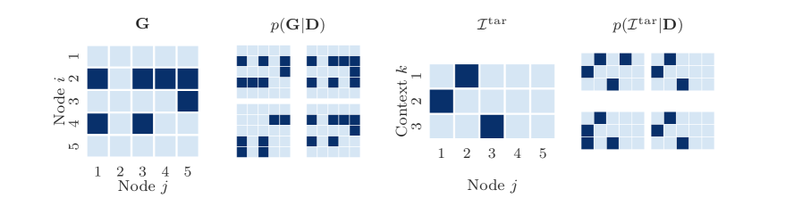
Figure 2: Instead of just one point estimate, BaCaDI yields particle approximations of the posteriors $p({\bf{G}}|\mathbf{D})$ and $p(\mathcal{I}^{\text{tar}}|\mathbf{D})$. We visually compare the posterior particles with the ground truth ${\bf{G}}$ and $\mathcal{I}^{\text{tar}}$ for a SF-2 graph with $d=5$ nodes and $M=3$ contexts. Blue colors represent edges or targets.

6 VARIATIONAL INFERENCE OVER CBNs AND INTERVENTIONS

In Section 5, we have presented an extended graphical model of the multi-context, unknown-intervention causal discovery problem. Our extended model introduces additional continuous variables ${\bf{Z}}$ and ${\bf{\Gamma}}$ that characterize the generative process of ${\bf{G}}$ and the intervention targets $\mathcal{I}^{\text{tar}}$. Proposition 1 shows that we can perform Bayesian inference of the graph ${\bf{G}}$ and intervention targets $\mathcal{I}^{\text{tar}}$ by inferring the posterior over the continuous latent variables ${\bf{Z}}$ and ${\bf{\Gamma}}$.

In this section, we discuss how to approach the final challenge of inferring this equally intractable, yet continuous posterior and finally convert the result back into an approximation of the joint posterior $p({\bf{G}},{\bf{\Theta}},\mathcal{I}^{\text{tar}},{\bf{\Theta}}_{\mathcal{I}}|\mathbf{D})$ over discrete structures ${\bf{G}},\mathcal{I}^{\text{tar}}$ and continuous parameters ${\bf{\Theta}},{\bf{\Theta}}_{\mathcal{I}}$.

Posterior scores. While Proposition 1 links the semi-continuous posterior $p({\bf{G}},{\bf{\Theta}},\mathcal{I}^{\text{tar}},{\bf{\Theta}}_{\mathcal{I}}|\mathbf{D})$ to its continuous counterpart, the inference problem appears just to shift. However, the transformation we introduce enables using inference methods based on continuous optimization, and more importantly, allows estimating the gradients of $\log p({\bf{Z}},{\bf{\Theta}},{\bf{\Gamma}},{\bf{\Theta}}_{\mathcal{I}}|\mathbf{D})$, which many approximate inference techniques rely on (e.g. Welling and Teh,, 2011; Chen et al.,, 2014; Liu and Wang,, 2016). The gradient with respect to ${\bf{\Gamma}}$ is given by

$$\begin{split}&\nabla_{{\bf{\Gamma}}}\log p({\bf{Z}},{\bf{\Theta}},{\bf{\Gamma}},{\bf{\Theta}}_{\mathcal{I}}|\mathbf{D})\\ &=\nabla_{{\bf{\Gamma}}}\log p({\bf{\Gamma}})+\frac{\nabla_{{\bf{\Gamma}}}\mathbb{E}_{p({\bf{G}}|{\bf{Z}})}\mathbb{E}_{p(\mathcal{I}^{\text{tar}}|{\bf{\Gamma}})}\left[\mathbf{\Psi}\right]}{\mathbb{E}_{p({\bf{G}}|{\bf{Z}})}\mathbb{E}_{p(\mathcal{I}^{\text{tar}}|{\bf{\Gamma}})}\left[\mathbf{\Psi}\right]}\end{split}$$ (12)

where $\mathbf{\Psi}$ the same as in Proposition 1 and contains the priors and likelihood in Eq. 11. By sampling ${\bf{G}}$ and $\mathcal{I}^{\text{tar}}$ using the Gumbel-softmax trick, we can pull the gradient $\nabla_{\bf{\Gamma}}$ inside the expectations and tractably approximate the score using Monte Carlo sampling. The gradients for ${\bf{Z}}$, ${\bf{\Theta}}$, and ${\bf{\Theta}}_{\mathcal{I}}$ are analogous. The derivations are given in Appendix A.3.

Consistent particle variational inference. To infer the latent posterior $p({\bf{Z}},{\bf{\Theta}},{\bf{\Gamma}},{\bf{\Theta}}_{\mathcal{I}}|\mathbf{D})$, we employ the particle variational inference approach Stein Variational Gradient Descent (SVGD) (Liu and Wang,, 2016). SVGD minimizes the KL divergence to the intractable distribution of interest using a finite, optimized set of particles. Specifically, the algorithm uses the score of the density to transport particles towards high-probability regions and a kernel $k(\cdot,\cdot)$ to introduce a repulsive force between the particles. Since BaCaDI allows estimating the score, we can apply SVGD off-the-shelf. We give an overview of SVGD in Appx. F.

Given $L$ initial particles $\{({\bf{Z}}^{(l)}_{0},{\bf{\Gamma}}^{(l)}_{0},{\bf{\Theta}}^{(l)}_{0},{\bf{\Theta}}^{(l)}_{\mathcal{I},0})\}_{l=1}^{L}$, we perform $T$ iterations of particle SVGD updates. We use annealing schedules $\alpha_{t}\rightarrow\infty$ and $\beta_{t}\rightarrow\infty$ for our continuous relaxations ${\bf{G}}_{\alpha}({\bf{Z}})$, $\mathcal{I}_{\alpha}^{\text{tar}}({\bf{\Gamma}})$ and the graph prior $p_{\beta}({\bf{Z}})$. By annealing the temperature parameters, our posterior over the continuous latent variables ${\bf{Z}}$ and ${\bf{\Gamma}}$ asymptotically converges into a probability distribution over discrete DAGs and interventions (proof in Appendix A.2).:

Proposition 2

As $\alpha\rightarrow\infty$ and $\beta\rightarrow\infty$ the posterior expectation in Prop. 1 converges to the simpler expression

$$\begin{split}\mathbb{E}_{p({\bf{G}},{\bf{\Theta}},\mathcal{I}^{\text{tar}},{\bf{\Theta}}_{\mathcal{I}}|\mathbf{D})}&[f({\bf{G}},{\bf{\Theta}},\mathcal{I}^{\text{tar}},{\bf{\Theta}}_{\mathcal{I}})]\\ \rightarrow\mathbb{E}_{p({\bf{Z}},{\bf{\Theta}},{\bf{\Gamma}},{\bf{\Theta}}_{\mathcal{I}}|\mathbf{D})}&[f({\bf{G}}_{\infty}({\bf{Z}}),{\bf{\Theta}},\mathcal{I}_{\infty}^{\text{tar}}({\bf{\Gamma}}),{\bf{\Theta}}_{\mathcal{I}})]\ \end{split}$$ (13)

with ${\bf{G}}_{\infty}({\bf{Z}})_{i,j}=\mathbf{1}_{\mathbf{u}_{i}^{\top}\mathbf{v}_{j}>0}$ and $\mathcal{I}_{\infty}^{\text{tar}}({\bf{\Gamma}})_{k,i}=\mathbf{1}_{\gamma_{i,k}>0}$. In the limit, the marginal posterior over discrete structures $p({\bf{G}},\mathcal{I}^{\text{tar}}|\mathbf{D})$ is supported on $\{\mathbf{G}|\mathbf{G}\in\{0,1\}^{d\times d}\wedge\mathbf{G}\text{ is acyclic}\}\times\{0,1\}^{M\times d}$ and, thus, a valid probability mass function over DAGs and intervention targets.

Proposition 2 states that, in the limit, the posterior expectation in (6) simplifies to (13) such that each particle maps to one DAG $\smash{{\bf{G}}_{\infty}({\bf{Z}}^{(l)}_{T})}$ and set of discrete targets $\smash{\mathcal{I}_{\infty}^{\text{tar}}({\bf{\Gamma}}_{T}^{(l)})}$. After completing the SVGD steps, we hence return the limit particles $\smash{{\bf{G}}_{\infty}({\bf{Z}}^{(l)}_{T})}$ and $\smash{\mathcal{I}_{\infty}^{\text{tar}}({\bf{\Gamma}}_{T}^{(l)})}$ as the particle approximation of the posterior $p({\bf{G}},{\bf{\Theta}},\mathcal{I}_{\text{tar}},{\bf{\Theta}}_{\mathcal{I}}|\mathbf{D})$. The full procedure is summarized in Algorithm 1 in Appx. B.

The behavior of SVGD guarantees the minimization of the KL divergence and asymptotic convergence to the continuous posterior $p({\bf{Z}},{\bf{\Theta}},{\bf{\Gamma}},{\bf{\Theta}}_{\mathcal{I}}|\mathbf{D})$ in the large sample limit of the number of particles (Liu,, 2017). By additionally annealing the continuous relaxations, the posterior that is approximated by SVGD converges to the semi-continuous posterior in Eq. 4 we are ultimately interested in. Together, we thus obtain an asymptotically consistent approximation of $p({\bf{G}},{\bf{\Theta}},\mathcal{I}^{\text{tar}},{\bf{\Theta}}_{\mathcal{I}}|\mathbf{D})$.

Identifiability. Our approach focuses on joint Bayesian inference over CBNs and interventions and applies to many instantiations of the generative process in (5). Under additional assumptions such as specific functional forms and noise distributions (Shimizu et al.,, 2006; Hoyer et al.,, 2008; Peters and Bühlmann,, 2014), identification results of related, non-Bayesian methods (e.g., Brouillard et al.,, 2020) apply to BaCaDI in the large sample limit where the posterior is dominated by the likelihood. By proposing an inference technique rather than a specific parametric model, theoretical results on identification are not of direct concern to us, similar to related algorithmic works on structure learning (Zheng et al.,, 2018; Yu et al.,, 2019; Lorch et al.,, 2021).

Figure 2 illustrates an example of the returned posterior particles for ${\bf{G}}$ and $\mathcal{I}^{\text{tar}}$ alongside the ground truth for data generated by a linear-Gaussian, five-node CBN. While SVGD yields a set of particles of with equal weights, we weight each particle by its unnormalized posterior probability $p({\bf{G}},{\bf{\Theta}},{\bf{\Theta}}_{\mathcal{I}},\mathcal{I}^{\text{tar}},|\mathbf{D})$ for performing approximate Bayesian model averaging, similar to Friedman et al., (1999). We find that this improves the empirical performance.

7 EXPERIMENTS

We evaluate BaCaDI on different causal discovery tasks with data from multiple contexts. Our goal is to empirically investigate how accurately BaCaDI predicts the causal structure as well as the intervention targets and how it compares to related state-of-the-art methods. First, we focus on synthetic datasets generated by CBNs. Second, we use the SERGIO simulator (Dibaeinia and Sinha,, 2020) to evaluate the methods on simulated gene expression data. In this more realistic setting, the methods operate under significant model misspecification, since the data-generating processes do not match the priors and likelihood.

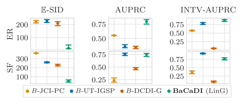
(a) Linear Gaussian

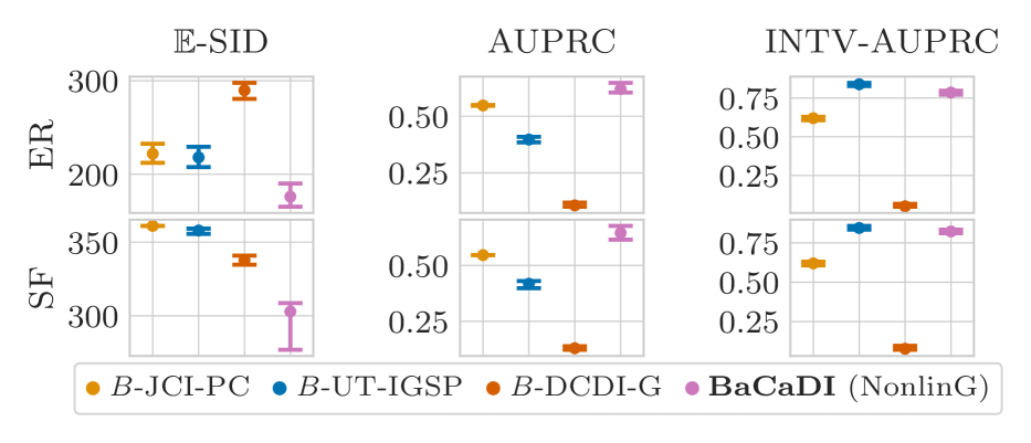
(b) Nonlinear Gaussian

Figure 3: Joint posterior inference over CBNs and interventions for linear and nonlinear Gaussian CBNs. The data is from ER-2 (top) and SF-2 (bottom) graphs with $d=20$ and $M=20$ contexts. BaCaDI consistently gives the best causal structure and intervention predictions. Lower values are better for $\mathbb{E}$-SID. Higher values are better for AUPRC/INTV-AUPRC.

7.1 Experimental Setup

Datasets. Following related work (Zheng et al.,, 2018; Yu et al.,, 2019; Zheng et al.,, 2020; Annadani et al.,, 2021; Scherrer et al.,, 2021; Lorch et al.,, 2021), we perform inference of randomly sampled graphs. We consider Erdős-Rényi  (Gilbert,, 1959) and scale-free (Barabási and Albert,, 1999) random graphs with $d=20$ nodes and $2d$ edges in expectation (ER-2 and SF-2). We create datasets by randomly sampling CBN parameters or simulating data with SERGIO. We then split the data into a dataset that is used to perform inference and held-out test datasets which are used to compute metrics. In all settings, we collect $n_{0}=100$ observational samples together with $n_{k}=10$ samples per intervention context for $k\in\{1,\dots,M\}$. This constitutes a low-sample setting commonly found in many applications. Further details on data generation are given in Appx. D.

Baselines. Since BaCaDI is a probabilistic method, we compare it to bootstrapped versions of existing algorithms that are capable of joint causal inference from multiple contexts with unknown interventions. We benchmark BaCaDI with constraint-based methods UT-IGSP (Squires et al.,, 2020) and the JCI framework with the PC algorithm (JCI-PC) (Mooij et al.,, 2016) and the score-based method DCDI (Brouillard et al.,, 2020), which can handle unknown interventions. JCI-PC and UT-IGSP are based on conditional independence or invariance tests. For DCDI, we use a neural network to model the local conditionals with Gaussian additive noise (DCDI-G). Since all of these methods infer only a single DAG estimate, we use the nonparametric DAG bootstrap approach (Friedman et al.,, 1999; Agrawal et al.,, 2019) to obtain an approximate distribution over DAGs and intervention targets. We report the baselines with a “B-" prefix to highlight that they are bootstrapped. Throughout the experiments, we use 20 bootstrap samples for all methods.

BaCaDI instantiations. We instantiate BaCaDI using 20 particles for SVGD, which matches the number of bootstrap samples of the baselines, and run it for 2000 steps of SVGD updates. In case a returned particle represents a cyclic graph, we drop the particle for the posterior approximation. Unless specified otherwise, we model interventions using a Gaussian likelihood $p_{i}^{I_{k}}({x}_{i}|{\bf{\Theta}}_{I_{k}})=\mathcal{N}(x_{i}|\mu^{I}_{k,i},\sigma_{I})$ with fixed variance ${\sigma_{I}}^{2}=0.5$. We infer the means ${\bf{\Theta}}_{I_{k}}=[\mu^{I}_{k,1},...,\mu^{I}_{k,d}]$ using a wide Gaussian prior $p({\bf{\Theta}}_{I_{k}}|I^{\text{tar}}_{k})=\prod_{i\in I^{\text{tar}}_{k}}p(\mu^{I}_{k,i}|I^{\text{tar}}_{k,i}=1)=\prod_{i\in I^{\text{tar}}_{k}}\mathcal{N}(\mu^{I}_{k,i}|0,10)$. This reflects an uninformative prior over a large effect range of the interventions. The conditionals for the observational likelihood are either modelled as linear or nonlinear models with additive Gaussian noise. The latter corresponds to the model of DCDI-G and uses 1 hidden-layer neural networks (NN) with $5$ hidden units. More details about the generative models can be found in Appx. D.1.

Metrics. Our reported metrics focus on three essential aspects of our inference problem: causal discovery, intervention detection, and inference of the full CBN for modeling the effects of interventions.

• Causal structure: The Structural Interventional Distance (SID) (Peters and Bühlmann,, 2015) quantifies the agreement between ${\bf{G}}$ and the true ${\bf{G}}_{\text{gt}}$ by the degree to which their adjustment sets coincide. Since we perform posterior inference, we report the expected SID: $\mathbb{E}\text{-SID}(p,{\bf{G}}_{\text{gt}}):=\sum_{{\bf{G}}}p({\bf{G}}|\mathcal{D})\cdot\text{SID}({\bf{G}},{\bf{G}}_{\text{gt}})$. UT-IGSP and JCI-PC only return a CPDAGs of the Interventional Markov Equivalence Class (I-MEC), so we calculate its lower and upper bound SID and use their midpoint in the $\mathbb{E}$-SID. We also report the area under the precision-recall curve (AUPRC) for individual edge predictions based on the posterior marginals $p(g_{ij}=1|\mathbf{D})$.

• Intervention targets: We report interventional AUPRC (INTV-AUPRC) for the detection of the individual target variables in each environment.

• Intervention effects: We report the average negative interventional log-likelihood (I-NLL) on $M^{\text{test}}=10$ heldout interventional datasets $\mathbf{D}^{\text{test}}=\{\mathcal{D}^{\text{test}}_{1},...,\mathcal{D}^{\text{test}}_{10}\}$, where different interventions are performed than in the training datasets. Each test dataset comprises 100 samples and has known intervention targets $I^{\text{tar}}_{\text{test},k}$ and effect distributions $p(x_{i}|{\bf{\Theta}}_{I_{\text{test},k}})$. Since UT-IGSP and JCI-PC do not learn the conditional distributions, we use the closed-form MLE parameters for a linear Gaussian model to compute the heldout I-NLL (Hauser and Bühlmann,, 2014).

Additional details on the metrics are given in Appendix  D.5.

Result aggregation. For all methods and settings, we perform a search over a specified range of hyperparameter using at least $20$ settings. For the specific choice of hyperparameters, we collect results over 30 different random task instances and pick the hyperparameters that resulted in the lowest I-NLL across the 30 instances in the held-out interventional dataset. We report the median of each metric together with its 90% confidence interval based on the empirical percentiles.

7.2 Experiment Results on Synthetic Data

In the synthetic data setting, we focus on hard interventions that set the values of the targeted variable to samples from a Gaussian with a randomly chosen mean bounded away from zero and a variance of $0.5$. Each interventional dataset is generated by intervening on a specific variable. We target all variables in the graph, i.e., the number of interventional contexts is $M=d$. In total, this results in $300$ samples for synthetic datasets with $d=20$ variables and $n_{0}=100,n_{k}=10$.

We first consider linear Gaussian CBNs, where each variable is a linear combination of its parents with additive Gaussian noise. The corresponding results for ER-2 and SF-2 are shown in Fig. 3(a). As a second task, we evaluate the setting of nonlinear Gaussian conditionals, where the mean of each variable given its parents is described by a neural network (NN) (see Appx. D.2 for details). Fig. 3(b) displays the results for nonlinear CBNs.

Across these four synthetic evaluation settings, BaCaDI’s causal structure predictions are the closest to the ground-truth CBN in terms of their intervention implications ($\mathbb{E}$-SID) and the prediction of individual edges (AUPRC). In most cases, our method outperforms the baselines by a significant margin. Moreover, BaCaDI achieves strong AUPRC scores for the prediction of intervention targets. Among the baselines, UT-IGSP is the best at detecting interventions, largely on par with BaCaDI. Although UT-IGSP also achieves high AUPRC for the linear SF-2 setting, the method performs significantly worse than BaCaDI in other settings and metrics. DCDI perfoms poorly in predicting the interventions and causal mechanisms.

In contrast to our fully Bayesian treatment of the joint posterior $p({\bf{G}},{\bf{\Theta}},\mathcal{I}^{\text{tar}}|\mathbf{D})$, the bootstrap baselines cannot propagate epistemic uncertainty between the inference of intervention targets and effects and inference of the CBN. This makes methods like DCDI, which does not regularize its neural network conditionals, prone to overfitting in small data settings, and may explain why BaCaDI is the only method to perform reliably in the low-sample regime.

Additional analyses. We perform additional experiments for $d=50$ node graphs as well as larger datasets. The results are shown in Fig.6-7 and 9 in Appx. E. In terms of scaling to larger graphs, BaCaDI is competitive to current state-of-the-art methods of causal discovery. For substantially larger graphs, the computational cost become prohibitively high when basing inference on SVGD. As an interesting use case, Appx. E.2 contains an ablation study investigating how BaCaDI can leverage interventional data compared to observational data, even when targets are unknown.

7.3 Experiments with Gene-Regulatory Networks

We evaluate all methods in a realistic application domain using SERGIO (Dibaeinia and Sinha,, 2020), a simulator for single-cell expression data of gene regulatory networks. Given a user-defined causal graph ${\bf{G}}$, SERGIO utilizes stochastic differential equations to simulate the gene expression dynamics and generate realistic single-cell transcriptomic datasets, which correspond to samples from the steady state of this dynamical system. Since real-world gene regulatory networks resemble scale-free structures (Albert,, 2005; Ouma et al.,, 2018), we use randomly sampled SF-2 graphs with $d=20$. In this domain, we perform $M=10$ gene knockout interventions on a single randomly selected target per context, resulting in a dataset size of $200$ including the observational samples. The data is standardized before inference. See Appx. D.3 for more details.

The Bayesian formulation allows BaCaDI to embed prior knowledge into the inference process in a principled manner. Since we perform knockout interventions, we expect intervention values to be close to zero and exhibit low variance. To reflect this belief, we set the intervention noise to ${\sigma_{I}}^{2}=0.01$ and use the prior $p(\mu^{I}_{k,i}|I^{\text{tar}}_{k,i}=1)=\mathcal{N}(\mu^{I}_{k,i}|0,1)$.

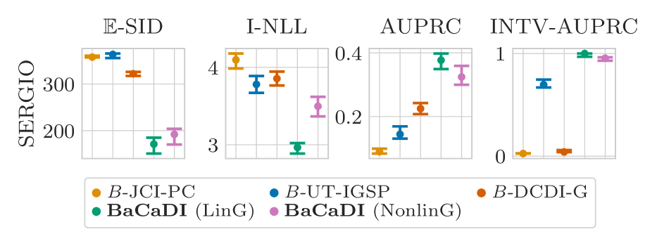
Figure 4: Joint posterior over CBNs and interventions for simulated gene expression data with $d=20$ and $M=10$ contexts. BaCaDI makes significantly better causal mechanism predictions than the baselines and accurately identifies the intervention targets. Lower values are better for $\mathbb{E}$-SID/I-NLL. Higher values are better for AUPRC/INTV-AUPRC.

Results. Fig. 4 shows the results for the SERGIO datasets. As in the synthetic CBN domain, BaCaDI infers the ground-truth graph most accurately. Moreover, our method is very accurate in predicting intervention targets as reflected by the intervention target AUPRC, where it benefits from the prior. In this context, the accuracy of JCI-PC is close to random guessing, predicting nearly no interventions and edges.

Since the data generated by SERGIO are samples from the steady state of a stochastic dynamical system, our Bayesian model from Sec. 5 is misspecified. The fact that BaCaDI still performs well demonstrates its robustness to model mismatch in practice. Overall, BaCaDI is able to make accurate causal structure predictions with only 200 simulated gene expression measurements from a challenging multi-experiment setting. This is a promising step towards joint causal inference in the life sciences. Here, the predicted intervention targets can further be of independent interest, e.g., for understanding off-target effects of drugs.

We believe that evaluating causal discovery methods beyond synthetic toy datasets on more realistic benchmarks, such as SERGIO, is an important direction for future research. In particular, there are many open questions about the practical applicability of current algorithms to real-world data. We refer to the work of Reisach et al., (2021) who discuss, in detail, potential issues that arise from synthetic benchmarking and the scale sensitivity of continuous optimization for causal structure learning.

8 DISCUSSION

In this work, we introduced BaCaDI, a fully-differentiable Bayesian causal discovery framework for data generated under various unknown interventional conditions. BaCaDI performs approximate inference jointly over the underlying causal graph, mechanisms, and the unknown interventions from multiple contexts. A key feature of BaCaDI is its principled end-to-end treatment of epistemic uncertainty. In our experiments, the naive bootstrapping of previous methods performs worse, potentially because the epistemic uncertainty does not propagate between the unknown interventions and the unknown causal Bayesian network. BaCaDI, on the other hand, operates reliably even when data is scarce, and can be instantiated with any parametric model as well as specific prior knowledge from domain experts.

While the Bayesian approach has shown promise in causal discovery, there are interesting open problems that remain. One is that the posterior becomes strongly intractable for graphs larger than five nodes, making it difficult to accurately characterize or quantify the quality of the posterior approximation. Additionally, since it is driven by the likelihood term, the posterior clusters data points based on their match to the observational likelihood or whether they require a separate likelihood. As a result, the performance of identifying interventions is improved when there is a stronger shift in distribution; interventions that only slightly alter the distribution cannot be detected with limited data.

Our work is motivated by the challenging problem of inferring the causal mechanisms of gene regulatory networks from real single-cell gene expression data. Our experimental results for the simulated gene expression data in Sec. 7.3 show that BaCaDI provides an important step towards achieving this goal. To ultimately reach it, future work needs to address a range of further challenges, such as dealing with the experimental measurement noise incurred by single-cell sequencing techniques.

Acknowledgments

This research was supported by the European Research Council (ERC) under the European Union’s Horizon 2020 research and innovation program grant agreement no. 815943 and the Swiss National Science Foundation under NCCR Automation, grant agreement 51NF40 180545. Jonas Rothfuss was supported by an Apple Scholars in AI/ML fellowship. We thank Parnian Kassraie for valuable feedback.

Appendix A PROOFS & DERIVATIONS

A.1 Latent Posterior (Proof of Proposition 1)

Recall that we have the generative model under which we factorize

$$p({\bf{Z}},{\bf{G}},{\bf{\Theta}},{\bf{\Gamma}},\mathcal{I},\mathbf{D}) =\underbrace{p({\bf{Z}})p({\bf{G}}|{\bf{Z}})p({\bf{\Theta}}|{\bf{G}})}_{\text{gen. process CBN}}\prod_{k=1}^{M}\underbrace{p({\bf{\Gamma}}_{k})p(I^{\text{tar}}_{k}|{\bf{\Gamma}}_{k})p({\bf{\Theta}}_{I_{k}}|I^{\text{tar}}_{k})}_{\text{gen. process interv.}}\underbrace{p(\mathcal{D}_{k}|{\bf{G}},{\bf{\Theta}},I^{\text{tar}}_{k},{\bf{\Theta}}_{I_{k}})}_{\text{interv. likelihood}}\vspace{-10pt}$$

where we write ${\bf{\Gamma}}:=[{\bf{\Gamma}}_{1},...,{\bf{\Gamma}}_{M}]$. For brevity, we can express this as

$$p({\bf{Z}},{\bf{G}},{\bf{\Theta}},{\bf{\Gamma}},\mathcal{I},\mathbf{D}) =p({\bf{Z}})p({\bf{G}}|{\bf{Z}})p({\bf{\Theta}}|{\bf{G}})\cdot p({\bf{\Gamma}})p(\mathcal{I}^{\text{tar}}|{\bf{\Gamma}})p({\bf{\Theta}}_{\mathcal{I}}|\mathcal{I}^{\text{tar}})\cdot p(\mathbf{D}|{\bf{G}},\mathcal{I},{\bf{\Theta}})\vspace{-10pt}$$

where $p(\mathbf{D}|{\bf{G}},\mathcal{I},{\bf{\Theta}})=p(\mathbf{D}|{\bf{G}},{\bf{\Theta}},\mathcal{I}^{\text{tar}},{\bf{\Theta}}_{\mathcal{I}})=\prod_{k=1}^{M}p(\mathcal{D}_{k}|{\bf{G}},{\bf{\Theta}},I^{\text{tar}}_{k},{\bf{\Theta}}_{I_{k}})$.

This gives us This gives us

$$\mathbb{E}_{p({\bf{G}},{\bf{\Theta}},\mathcal{I}|\mathbf{D})}[f({\bf{G}},{\bf{\Theta}},\mathcal{I})]$$

$$=\sum_{{\bf{G}}}\int_{\bf{\Theta}}\sum_{\mathcal{I}^{\text{tar}}}\int_{{\bf{\Theta}}_{\mathcal{I}}}p({\bf{G}},{\bf{\Theta}},\mathcal{I}|\mathbf{D})f({\bf{G}},{\bf{\Theta}},\mathcal{I})d{\bf{\Theta}}d{\bf{\Theta}}_{\mathcal{I}}$$

$$=\sum_{{\bf{G}}}\int_{\bf{\Theta}}\sum_{\mathcal{I}^{\text{tar}}}\int_{{\bf{\Theta}}_{\mathcal{I}}}p({\bf{G}},\mathcal{I}^{\text{tar}},{\bf{\Theta}},{\bf{\Theta}}_{\mathcal{I}}|\mathbf{D})f({\bf{G}},{\bf{\Theta}},\mathcal{I})d{\bf{\Theta}}d{\bf{\Theta}}_{\mathcal{I}}$$

$$(\text{splitting }\mathcal{I}\text{ to }\mathcal{I}^{\text{tar}},{\bf{\Theta}}_{\mathcal{I}})$$

$$=\sum_{{\bf{G}}}\int_{\bf{\Theta}}\sum_{\mathcal{I}^{\text{tar}}}\int_{{\bf{\Theta}}_{\mathcal{I}}}\frac{p({\bf{G}},\mathcal{I}^{\text{tar}},{\bf{\Theta}},{\bf{\Theta}}_{\mathcal{I}},\mathbf{D})f({\bf{G}},{\bf{\Theta}},\mathcal{I})}{p(\mathbf{D})}d{\bf{\Theta}}d{\bf{\Theta}}_{\mathcal{I}}$$

$$=\sum_{{\bf{G}}}\int_{\bf{\Theta}}\sum_{\mathcal{I}^{\text{tar}}}\int_{{\bf{\Theta}}_{\mathcal{I}}}\int_{\bf{Z}}\int_{\bf{\Gamma}}\frac{p({\bf{Z}},{\bf{G}},{\bf{\Gamma}},\mathcal{I}^{\text{tar}},{\bf{\Theta}},{\bf{\Theta}}_{\mathcal{I}},\mathbf{D})f({\bf{G}},{\bf{\Theta}},\mathcal{I})}{p(\mathbf{D})}d{\bf{Z}}d{\bf{\Gamma}}d{\bf{\Theta}}d{\bf{\Theta}}_{\mathcal{I}}$$

$$(\text{extending by }{\bf{Z}},{\bf{\Gamma}})$$

$$=\int_{{\bf{Z}},{\bf{\Gamma}},{\bf{\Theta}},{\bf{\Theta}}_{\mathcal{I}}}\sum_{{\bf{G}},\mathcal{I}^{\text{tar}}}\frac{p({\bf{Z}},{\bf{G}},{\bf{\Gamma}},\mathcal{I}^{\text{tar}},{\bf{\Theta}},{\bf{\Theta}}_{\mathcal{I}},\mathbf{D})f({\bf{G}},{\bf{\Theta}},\mathcal{I})}{p(\mathbf{D})}d{\bf{Z}}d{\bf{\Gamma}}d{\bf{\Theta}}d{\bf{\Theta}}_{\mathcal{I}}$$

$$(\text{rearranging})$$

$$=\int_{{\bf{Z}},{\bf{\Gamma}},{\bf{\Theta}},{{\bf{\Theta}}_{\mathcal{I}}}}\sum_{{\bf{G}},\mathcal{I}^{\text{tar}}}\frac{p({\bf{Z}})p({\bf{G}}|{\bf{Z}})p({\bf{\Theta}}|{\bf{G}})p({\bf{\Gamma}})p(\mathcal{I}^{\text{tar}}|{\bf{\Gamma}})p({\bf{\Theta}}_{\mathcal{I}}|\mathcal{I}^{\text{tar}})p(\mathbf{D}|{\bf{G}},\mathcal{I},{\bf{\Theta}})f({\bf{G}},{\bf{\Theta}},\mathcal{I})}{p(\mathbf{D})}d{\bf{Z}}d{\bf{\Gamma}}d{\bf{\Theta}}d{\bf{\Theta}}_{\mathcal{I}}$$

$$(\text{by the generative model})$$

$$=E_{p({\bf{Z}},{\bf{\Theta}},{\bf{\Gamma}},{\bf{\Theta}}_{\mathcal{I}}|\mathbf{D})}\left[\sum_{{\bf{G}},\mathcal{I}^{\text{tar}}}\frac{p({\bf{G}}|{\bf{Z}})p({\bf{\Theta}}|{\bf{G}})p(\mathcal{I}^{\text{tar}}|{\bf{\Gamma}})p({\bf{\Theta}}_{\mathcal{I}}|\mathcal{I}^{\text{tar}})p(\mathbf{D}|{\bf{G}},\mathcal{I},{\bf{\Theta}})f({\bf{G}},{\bf{\Theta}},\mathcal{I})}{p({\bf{\Theta}},{\bf{\Theta}}_{\mathcal{I}},\mathbf{D}|{\bf{Z}},{\bf{\Gamma}})}\right]$$

$$(\text{since }p({\bf{Z}},{\bf{\Theta}},{\bf{\Gamma}},{\bf{\Theta}}_{\mathcal{I}}|\mathbf{D})=\frac{p({\bf{Z}})p({\bf{\Gamma}})p({\bf{\Theta}},{\bf{\Theta}}_{\mathcal{I}},\mathbf{D}|{\bf{Z}},{\bf{\Gamma}})}{p(\mathbf{D})})$$

$$=E_{p({\bf{Z}},{\bf{\Theta}},{\bf{\Gamma}},{\bf{\Theta}}_{\mathcal{I}}|\mathbf{D})}\left[\frac{\sum_{{\bf{G}},\mathcal{I}^{\text{tar}}}p({\bf{G}}|{\bf{Z}})p({\bf{\Theta}}|{\bf{G}})p(\mathcal{I}^{\text{tar}}|{\bf{\Gamma}})p({\bf{\Theta}}_{\mathcal{I}}|\mathcal{I}^{\text{tar}})p(\mathbf{D}|{\bf{G}},\mathcal{I},{\bf{\Theta}})f({\bf{G}},{\bf{\Theta}},\mathcal{I})}{p({\bf{\Theta}},{\bf{\Theta}}_{\mathcal{I}},\mathbf{D}|{\bf{Z}},{\bf{\Gamma}})}\right]$$

$$(\text{rearranging )}$$

$$=E_{p({\bf{Z}},{\bf{\Theta}},{\bf{\Gamma}},{\bf{\Theta}}_{\mathcal{I}}|\mathbf{D})}\left[\frac{\sum_{{\bf{G}},\mathcal{I}^{\text{tar}}}p({\bf{G}}|{\bf{Z}})p({\bf{\Theta}}|{\bf{G}})p(\mathcal{I}^{\text{tar}}|{\bf{\Gamma}})p({\bf{\Theta}}_{\mathcal{I}}|\mathcal{I}^{\text{tar}})p(\mathbf{D}|{\bf{G}},\mathcal{I},{\bf{\Theta}})f({\bf{G}},{\bf{\Theta}},\mathcal{I})}{\sum_{{\bf{G}},\mathcal{I}^{\text{tar}}}p({\bf{G}},\mathcal{I}^{\text{tar}},{\bf{\Theta}},{\bf{\Theta}}_{\mathcal{I}},\mathbf{D}|{\bf{Z}},{\bf{\Gamma}})}\right]$$

$$(\text{law of total probability )}$$

$$=\mathbb{E}_{p({\bf{Z}},{\bf{\Theta}},{\bf{\Gamma}},{\bf{\Theta}}_{\mathcal{I}}|\mathbf{D})}\left[\frac{\sum_{{\bf{G}},\mathcal{I}^{\text{tar}}}p({\bf{G}}|{\bf{Z}})p({\bf{\Theta}}|{\bf{G}})p(\mathcal{I}^{\text{tar}}|{\bf{\Gamma}})p({\bf{\Theta}}_{\mathcal{I}}|\mathcal{I}^{\text{tar}})p(\mathbf{D}|{\bf{G}},\mathcal{I},{\bf{\Theta}})f({\bf{G}},{\bf{\Theta}},\mathcal{I})}{\sum_{{\bf{G}},\mathcal{I}^{\text{tar}}}p({\bf{G}}|{\bf{Z}})p({\bf{\Theta}}|{\bf{G}})p(\mathcal{I}^{\text{tar}}|{\bf{\Gamma}})p({\bf{\Theta}}_{\mathcal{I}}|\mathcal{I}^{\text{tar}})p(\mathbf{D}|{\bf{G}},\mathcal{I},{\bf{\Theta}})}\right]$$

$$(\text{by the generative model )}$$

$$=\mathbb{E}_{p({\bf{Z}},{\bf{\Theta}},{\bf{\Gamma}},{\bf{\Theta}}_{\mathcal{I}}|\mathbf{D})}\left[\frac{\mathbb{E}_{p({\bf{G}}|{\bf{Z}}),p(\mathcal{I}^{\text{tar}}|{\bf{\Gamma}})}[f({\bf{G}},{\bf{\Theta}},\mathcal{I})p({\bf{\Theta}}|{\bf{G}})p({\bf{\Theta}}_{\mathcal{I}}|\mathcal{I}^{\text{tar}})p(\mathbf{D}|{\bf{G}},\mathcal{I},{\bf{\Theta}})]}{\mathbb{E}_{p({\bf{G}}|{\bf{Z}}),p(\mathcal{I}^{\text{tar}}|{\bf{\Gamma}})}[p({\bf{\Theta}}|{\bf{G}})p({\bf{\Theta}}_{\mathcal{I}}|\mathcal{I}^{\text{tar}})p(\mathbf{D}|{\bf{G}},\mathcal{I},{\bf{\Theta}})]}\right]$$

$\square$

A.2 Annealing the Posterior (Proof of Proposition 2)

The latent variables ${\bf{Z}}$ and ${\bf{\Gamma}}$ probabilistically model the causal graph ${\bf{G}}$ and intervention target masks $\mathcal{I}^{\text{tar}}$. In a similar way, they can be viewed as as continuous relaxations of ${\bf{G}}$ and $\mathcal{I}^{\text{tar}}$ respectively, where the $\alpha$ trades-off between smoothness and accuracy of these relaxations. If $\alpha\rightarrow\infty$, the sigmoid $\sigma_{\alpha}(\cdot)$ converges to the unit step function so that the probability distributions

$$p({\bf{G}}_{i,j}|{\bf{Z}}) =p({\bf{G}}_{i,j}|\mathbf{u}_{i},\mathbf{v}_{j})=\mathbf{1}_{(\mathbf{u}_{i}^{\top}\mathbf{v}_{j}>0)={\bf{G}}_{i,j}}~{},\text{and}$$ (14)

$$p(I^{\text{tar}}_{k,i}|{\bf{\Gamma}}) =p(I^{\text{tar}}_{k,i}|\gamma_{k,i})=\mathbf{1}_{(\gamma_{i,k}>0)=I^{\text{tar}}_{k,i}}$$ (15)

become deterministic indicator functions, representing only single discrete graph ${\bf{G}}_{\infty}({\bf{Z}})\in\{0,1\}^{d\times d}$ and target mask $\mathcal{I}_{\infty}^{\text{tar}}({\bf{\Gamma}})\in\{0,1\}^{M\times d}$. Since, the probability distributions $p({\bf{G}}|{\bf{Z}})$ and $p(\mathcal{I}^{\text{tar}}|{\bf{\Gamma}})$ converge to indicator function, they allow us to simplify the expectation in Proposition 1 as follows:

$$\begin{split}&\mathbb{E}_{p({\bf{G}},{\bf{\Theta}},\mathcal{I},{\bf{\Theta}}_{\mathcal{I}}|\mathbf{D})}[f({\bf{G}},{\bf{\Theta}},\mathcal{I},{\bf{\Theta}}_{\mathcal{I}})]\\ &=\mathbb{E}_{p({\bf{Z}},{\bf{\Theta}},{\bf{\Gamma}},{\bf{\Theta}}_{\mathcal{I}}|\mathbf{D})}\left[\frac{\mathbb{E}_{p({\bf{G}}|{\bf{Z}}),p(\mathcal{I}^{\text{tar}}|{\bf{\Gamma}})}[f({\bf{G}},{\bf{\Theta}},\mathcal{I},{\bf{\Theta}}_{\mathcal{I}})p({\bf{\Theta}}|{\bf{G}})p({\bf{\Theta}}_{\mathcal{I}}|\mathcal{I}^{\text{tar}})p(\mathbf{D}|{\bf{G}},\mathcal{I},{\bf{\Theta}})]}{\mathbb{E}_{p({\bf{G}}|{\bf{Z}}),p(\mathcal{I}^{\text{tar}}|{\bf{\Gamma}})}[p({\bf{\Theta}}|{\bf{G}})p({\bf{\Theta}}_{\mathcal{I}}|\mathcal{I}^{\text{tar}})p(\mathbf{D}|{\bf{G}},\mathcal{I},{\bf{\Theta}})]}\right]\\ \\ &\rightarrow\mathbb{E}_{p({\bf{Z}},{\bf{\Theta}},{\bf{\Gamma}},{\bf{\Theta}}_{\mathcal{I}}|\mathbf{D})}[f({\bf{G}}_{\infty}({\bf{Z}}),{\bf{\Theta}},\mathcal{I}_{\infty}^{\text{tar}}({\bf{\Gamma}}),{\bf{\Theta}}_{\mathcal{I}})]\;.\end{split}$$ (16)

This holds since the inner expectations evaluate to a single point for $\alpha\rightarrow\infty$ and thus cancel out.

If additionally the inverse temperature parameter in the latent prior $p_{\beta}({\bf{Z}})$ goes to infinity, i.e., $\beta\rightarrow\infty$, $p_{\beta}({\bf{Z}})$, the support of $p_{\beta}({\bf{Z}})=p_{\beta}(\mathbf{U},\mathbf{V})$ reduces to the set $\text{supp}(p_{\infty}({\bf{Z}}))=\{{\bf{Z}}|{\bf{Z}}\in\mathbb{R}^{2\times d\times d}\wedge h({\bf{G}}_{\infty}({\bf{Z}}))=0\}$. In particular, the prior only assigns non-zero probabilities to latent variables ${\bf{Z}}$ that correspond to acyclical graphs ${\bf{G}}_{\infty}({\bf{Z}})$. Since the posterior $p({\bf{Z}},{\bf{G}},{\bf{\Theta}},{\bf{\Gamma}},\mathcal{I}^{\text{tar}},{\bf{\Theta}}_{\mathcal{I}}|\mathbf{D})$ depends multiplicatively on $p_{\beta}({\bf{Z}})$ (see Eq. 5), the support of

$$p({\bf{G}},\mathcal{I}^{\text{tar}}|\mathbf{D})=\int_{{\bf{Z}},{\bf{\Gamma}},{\bf{\Theta}},{\bf{\Theta}}_{\mathcal{I}}}p({\bf{Z}},{\bf{G}},{\bf{\Theta}},{\bf{\Gamma}},\mathcal{I}^{\text{tar}},{\bf{\Theta}}_{\mathcal{I}}|\mathbf{D})d{\bf{Z}}d{\bf{\Gamma}}d{\bf{\Theta}}d{\bf{\Theta}}_{\mathcal{I}}$$ (17)

asymptotically becomes a subset of $\{\mathbf{G}|\mathbf{G}\in\{0,1\}^{n\times n}\wedge\mathbf{G}\text{ is acyclic}\}\times\{0,1\}^{M\times d}$ since $h({\bf{G}})=0\Leftrightarrow{\bf{G}}\text{ is acyclic}$.

A.3 Scores

In this section, we show how to derive the score, i.e. the gradient of the log-posterior, of our model introduced in Sec. 5.

The score w.r.t. auxiliary variables ${\bf{Z}}$ and ${\bf{\Gamma}}$ requires marginalization over the corresponding discrete structures ${\bf{G}}$ and $\mathcal{I}^{\text{tar}}$ as given by

$$\nabla_{{\bf{Z}}}\log p({\bf{Z}},{\bf{\Theta}},{\bf{\Gamma}},{\bf{\Theta}}_{\mathcal{I}}|\mathbf{D})=\nabla_{{\bf{Z}}}\log p({\bf{Z}})+\frac{\nabla_{{\bf{Z}}}\mathbb{E}_{p({\bf{G}}|{\bf{Z}})}\mathbb{E}_{p(\mathcal{I}^{\text{tar}}|{\bf{\Gamma}})}\left[p({\bf{\Theta}},{\bf{\Theta}}_{\mathcal{I}},\mathbf{D}|{\bf{G}},\mathcal{I}^{\text{tar}})\right]}{\mathbb{E}_{p({\bf{G}}|{\bf{Z}})}\mathbb{E}_{p(\mathcal{I}^{\text{tar}}|{\bf{\Gamma}})}\left[p({\bf{\Theta}},{\bf{\Theta}}_{\mathcal{I}},\mathbf{D}|{\bf{G}},\mathcal{I}^{\text{tar}})\right]}\;,$$ (18)

$$\nabla_{{\bf{\Gamma}}}\log p({\bf{Z}},{\bf{\Theta}},{\bf{\Gamma}},{\bf{\Theta}}_{\mathcal{I}}|\mathbf{D})=\nabla_{{\bf{\Gamma}}}\log p({\bf{\Gamma}})+\frac{\nabla_{{\bf{\Gamma}}}\mathbb{E}_{p({\bf{G}}|{\bf{Z}})}\mathbb{E}_{p(\mathcal{I}^{\text{tar}}|{\bf{\Gamma}})}\left[p({\bf{\Theta}},{\bf{\Theta}}_{\mathcal{I}},\mathbf{D}|{\bf{G}},\mathcal{I}^{\text{tar}})\right]}{\mathbb{E}_{p({\bf{G}}|{\bf{Z}})}\mathbb{E}_{p(\mathcal{I}^{\text{tar}}|{\bf{\Gamma}})}\left[p({\bf{\Theta}},{\bf{\Theta}}_{\mathcal{I}},\mathbf{D}|{\bf{G}},\mathcal{I}^{\text{tar}})\right]}\;.$$ (19)

where, $p({\bf{\Theta}},{\bf{\Theta}}_{\mathcal{I}},\mathbf{D}|{\bf{G}},\mathcal{I}^{\text{tar}})=p({\bf{\Theta}}|{\bf{G}})\prod_{k=1}^{m}p(\mathcal{D}_{k}|{\bf{G}},{\bf{\Theta}},I^{\text{tar}}_{k},{\bf{\Theta}}_{I_{k}})p({\bf{\Theta}}_{I_{k}}|I^{\text{tar}}_{k})$.

The expectations in Eq. 18 and Eq. 19 can be estimated and differentiated by sampling the intervention masks $\mathcal{I}^{\text{tar}}\sim\text{Bern}\left(\sigma_{\alpha}({\bf{\Gamma}})\right)$ and the adjacency matrices ${\bf{G}}\sim\text{Bern}\left(\sigma_{\alpha}(\mathbf{U}\mathbf{V}^{\top})\right)$ using the Gumbel-Softmax trick (Jang et al.,, 2016; Maddison et al.,, 2017). For obtaining a differentiable log-likelihood, we mask individual log-likelihood summands based on ${\bf{G}}$ (Lorch et al.,, 2021) and use the intervention masks $\mathcal{I}^{\text{tar}}$ to select between observational and interventional log-likelihood (cf. Eq. 11).

To see how the above equations hold, we show the derivations in the following. We start the derivations with the unnormalized posterior since

$$\nabla_{{\bf{Z}}}\log p({\bf{Z}},{\bf{\Gamma}},{\bf{\Theta}},{\bf{\Theta}}_{\mathcal{I}}|\mathcal{D})= \nabla_{{\bf{Z}}}\log p({\bf{Z}},{\bf{\Gamma}},{\bf{\Theta}},{\bf{\Theta}}_{\mathcal{I}},\mathcal{D})-\nabla_{{\bf{Z}}}\log p(\mathcal{D})$$ (20)

$$= \nabla_{{\bf{Z}}}\log p({\bf{Z}},{\bf{\Gamma}},{\bf{\Theta}},{\bf{\Theta}}_{\mathcal{I}},\mathcal{D})$$ (21)

and analogously for the gradients w.r.t. to other variables ${\bf{Z}},{\bf{\Gamma}},{\bf{\Theta}},{\bf{\Theta}}_{\mathcal{I}}$ .

By basic rules of probability theory and using the identity $\nabla_{\mathbf{x}}\log p({\mathbf{x}})=\nabla_{\mathbf{x}}p({\mathbf{x}})/p({\mathbf{x}})$, we obtain

$$\nabla_{{\bf{Z}}}\log p({\bf{Z}},{\bf{\Gamma}},{\bf{\Theta}}, {\bf{\Theta}}_{\mathcal{I}},\mathbf{D})=$$ (22)

$$= \nabla_{{\bf{Z}}}\log p({\bf{Z}})+\nabla_{{\bf{Z}}}\log p({\bf{\Theta}},{\bf{\Theta}}_{\mathcal{I}},\mathbf{D}|{\bf{Z}},{\bf{\Gamma}})$$ (23)

$$= \nabla_{{\bf{Z}}}\log p({\bf{Z}})+\frac{\nabla_{{\bf{Z}}}p({\bf{\Theta}},{\bf{\Theta}}_{\mathcal{I}},\mathbf{D}|{\bf{Z}},{\bf{\Gamma}})}{p({\bf{\Theta}},{\bf{\Theta}}_{\mathcal{I}},\mathbf{D}|{\bf{Z}},{\bf{\Gamma}})}$$ (24)

$$= \nabla_{{\bf{Z}}}\log p({\bf{Z}})+\frac{\nabla_{{\bf{Z}}}\left[\sum_{{\bf{G}}}\sum_{\mathcal{I}^{\text{tar}}}p({\bf{G}}|{\bf{Z}})p(\mathcal{I}^{\text{tar}}|{\bf{\Gamma}})p({\bf{\Theta}},{\bf{\Theta}}_{\mathcal{I}},\mathbf{D}|{\bf{G}},\mathcal{I}^{\text{tar}})\right]}{\sum_{{\bf{G}}}\sum_{\mathcal{I}^{\text{tar}}}p({\bf{G}}|{\bf{Z}})p(\mathcal{I}^{\text{tar}}|{\bf{\Gamma}})p({\bf{\Theta}},{\bf{\Theta}}_{\mathcal{I}},\mathbf{D}|{\bf{G}},\mathcal{I}^{\text{tar}})}$$ (25)

$$= \nabla_{{\bf{Z}}}\log p({\bf{Z}})+\frac{\nabla_{{\bf{Z}}}\mathbb{E}_{p({\bf{G}}|{\bf{Z}})}\mathbb{E}_{p(\mathcal{I}^{\text{tar}}|{\bf{\Gamma}})}\left[p({\bf{\Theta}},{\bf{\Theta}}_{\mathcal{I}},\mathbf{D}|{\bf{G}},\mathcal{I}^{\text{tar}})\right]}{\mathbb{E}_{p({\bf{G}}|{\bf{Z}})}\mathbb{E}_{p(\mathcal{I}^{\text{tar}}|{\bf{\Gamma}})}\left[p({\bf{\Theta}},{\bf{\Theta}}_{\mathcal{I}},\mathbf{D}|{\bf{G}},\mathcal{I}^{\text{tar}})\right]}$$ (26)

and analogously

$$\nabla_{{\bf{\Gamma}}}\log p({\bf{Z}},{\bf{\Gamma}},{\bf{\Theta}}, {\bf{\Theta}}_{\mathcal{I}},\mathbf{D})=$$ (27)

$$= \nabla_{{\bf{\Gamma}}}\log p({\bf{\Gamma}})+\nabla_{{\bf{\Gamma}}}\log p({\bf{\Theta}},{\bf{\Theta}}_{\mathcal{I}},\mathbf{D}|{\bf{Z}},{\bf{\Gamma}})$$ (28)

$$= \nabla_{{\bf{\Gamma}}}\log p{\bf{\Gamma}})+\frac{\nabla_{{\bf{\Gamma}}}p({\bf{\Theta}},{\bf{\Theta}}_{\mathcal{I}},\mathbf{D}|{\bf{Z}},{\bf{\Gamma}})}{p({\bf{\Theta}},{\bf{\Theta}}_{\mathcal{I}},\mathbf{D}|{\bf{Z}},{\bf{\Gamma}})}$$ (29)

$$= \nabla_{{\bf{\Gamma}}}\log p({\bf{\Gamma}})+\frac{\nabla_{{\bf{\Gamma}}}\left[\sum_{{\bf{G}}}\sum_{\mathcal{I}^{\text{tar}}}p({\bf{G}}|{\bf{Z}})p(\mathcal{I}^{\text{tar}}|{\bf{\Gamma}})p({\bf{\Theta}},{\bf{\Theta}}_{\mathcal{I}},\mathbf{D}|{\bf{G}},\mathcal{I}^{\text{tar}})\right]}{\sum_{{\bf{G}}}\sum_{\mathcal{I}^{\text{tar}}}p({\bf{G}}|{\bf{Z}})p(\mathcal{I}^{\text{tar}}|{\bf{\Gamma}})p({\bf{\Theta}},{\bf{\Theta}}_{\mathcal{I}},\mathbf{D}|{\bf{G}},\mathcal{I}^{\text{tar}})}$$ (30)

$$= \nabla_{{\bf{\Gamma}}}\log p({\bf{\Gamma}})+\frac{\nabla_{{\bf{\Gamma}}}\mathbb{E}_{p({\bf{G}}|{\bf{Z}})}\mathbb{E}_{p(\mathcal{I}^{\text{tar}}|{\bf{\Gamma}})}\left[p({\bf{\Theta}},{\bf{\Theta}}_{\mathcal{I}},\mathbf{D}|{\bf{G}},\mathcal{I}^{\text{tar}})\right]}{\mathbb{E}_{p({\bf{G}}|{\bf{Z}})}\mathbb{E}_{p(\mathcal{I}^{\text{tar}}|{\bf{\Gamma}})}\left[p({\bf{\Theta}},{\bf{\Theta}}_{\mathcal{I}},\mathbf{D}|{\bf{G}},\mathcal{I}^{\text{tar}})\right]}\;.$$ (31)

Appendix B ALGORITHM DETAILS

B.1 Annealing Schedule

As described in Sec. A.2, we anneal $\alpha_{t}$ such that $\alpha_{t}\rightarrow\infty$ and, at terminal iteration of the SVGD training loop, convert ${\bf{Z}}$ and ${\bf{\Gamma}}$ into their discrete counterparts ${\bf{G}}_{\infty}({\bf{Z}})$ and $\mathcal{I}_{\infty}^{\text{tar}}({\bf{\Gamma}})$. Similarly, we set an annealing schedule $\beta_{t}\rightarrow\infty$ for inverse temperature parameter in the latent prior $p_{\beta}({\bf{Z}})$ such that we only model DAGs as the training progresses.

The annealing schedule for both $\alpha_{t}$ and $\beta_{t}$is a simple linear schedule, i.e. we put $\alpha_{t}=t\cdot\alpha$ and $\beta_{t}=t\cdot\beta$ for scale values $\alpha,\beta>0$ where $t$ is the step in the SVGD inference (see B). For all results in the main text, we fix $\alpha=0.01$ and $\beta=2$. These values were empirically found to be the best trade-off between smoothness and accuracy of the relaxations during the inference process.

B.2 SVGD Kernel

In our experiments, we employ an additive RBF kernel. We also considered a product of RBF kernels, though, found that the additive kernel composition performed better. This additive kernel is defined as

$$\begin{split}k\left(({\bf{Z}},{\bf{\Theta}},{\bf{\Gamma}},{\bf{\Theta}}_{\mathcal{I}}),({\bf{Z}}^{\prime},{\bf{\Theta}}^{\prime},{\bf{\Gamma}}^{\prime},{\bf{\Theta}}_{\mathcal{I}}^{\prime})\right):=&\exp\left(-\frac{\lVert{\bf{Z}}-{\bf{Z}}^{\prime}\rVert^{2}}{2\tau_{Z}}\right)+\exp\left(-\frac{\lVert{\bf{\Gamma}}-{\bf{\Gamma}}^{\prime}\rVert^{2}}{2\tau_{\gamma}}\right)\\ +&\exp\left(-\frac{\lVert{\bf{\Theta}}-{\bf{\Theta}}^{\prime}\rVert^{2}}{2\tau_{\theta}}\right)+\exp\left(-\frac{\lVert{\bf{\Theta}}_{\mathcal{I}}-{\bf{\Theta}}_{\mathcal{I}}^{\prime}\rVert^{2}}{2\tau_{\theta}}\right)\end{split}$$ (32)

with lengthscales $\tau_{Z},\tau_{\gamma},\tau_{\theta}$. For brevity, we also write $k(\mathbf{\Omega},\mathbf{\Omega}^{\prime})$ for (32) where $\mathbf{\Omega}:=({\bf{Z}},{\bf{\Theta}},{\bf{\Gamma}},{\bf{\Theta}}_{\mathcal{I}})$. For SVGD, the kernel introduces repulsive forces which make the particles disperse well across the domain (see F).

B.3 Algorithm overview

We provide a pseudocode of our algorithm with its SVGD instantiation in Alg. 1.

Algorithm 1 BaCaDI with SVGD for inference of $p({\bf{G}},{\bf{\Theta}},\mathcal{I}^{\text{tar}},{\bf{\Theta}}_{\mathcal{I}}|\mathbf{D})$

Input: Set of datasets $\mathbf{D}=\{\mathcal{D}_{0},...,\mathcal{D}_{M}\}$ from the same causal system under different contexts
      Input: Kernel $k$, schedules for $\alpha_{t},\beta_{t}$, and stepsizes $\eta_{t}$
      Output: Set of CBN and intervention particles $\{({\bf{G}}^{(l)},{\bf{\Theta}}^{(l)},\mathcal{I}^{\text{tar},(l)},{\bf{\Theta}}^{(l)}_{\mathcal{I}})\}_{l=1}^{L}$

1:Initialize set of latent and parameter particles $\{\mathbf{\Omega}^{(l)}_{0}\}_{l=1}^{L}=\{({\bf{Z}}^{(l)}_{0},{\bf{\Gamma}}^{(l)}_{0},{\bf{\Theta}}^{(l)}_{0},{\bf{\Theta}}^{(l)}_{\mathcal{I},0})\}_{l=1}^{L}$

2:for iteration $t=0$ to $T-1$ do

3:     Estimate $\nabla\log p({\bf{Z}},{\bf{\Theta}},{\bf{\Gamma}},{\bf{\Theta}}_{\mathcal{I}}|\mathbf{D})$ for each $\mathbf{\Omega}^{(l)}_{t}=({\bf{Z}}^{(l)}_{t},{\bf{\Theta}}^{(l)}_{t},{\bf{\Gamma}}^{(l)}_{t},{\bf{\Theta}}^{(l)}_{\mathcal{I},t})$ $\triangleright$ see Eq 18, 19

4:     for particle $m=l$ to $L$ do

5:         $\displaystyle{\bf{Z}}^{(l)}_{t+1}\leftarrow{\bf{Z}}^{(l)}_{t}+\eta_{t}~{}\bm{\phi}^{{\bf{Z}}}_{t}(\mathbf{\Omega}^{(l)}_{t})$ $\triangleright$ SVGD steps

6:    where $\displaystyle\bm{\phi}^{{\bf{Z}}}_{t}(\cdot):=\frac{1}{L}\sum_{l=L}^{M}\Big{[}k\left(\mathbf{\Omega}^{(l)}_{t},~{}\cdot~{}\right)~{}\nabla_{{\bf{Z}}^{(l)}_{t}}\log p(\mathbf{\Omega}^{(l)}_{t}|\mathbf{D})+\nabla_{{\bf{Z}}^{(l)}_{t}}k\left(\mathbf{\Omega}^{(l)}_{t},~{}\cdot~{}\right)\Big{]}$

7:         $\displaystyle{\bf{\Theta}}^{(l)}_{t+1}\leftarrow{\bf{\Theta}}^{(l)}_{t}+\eta_{t}~{}\bm{\phi}^{{\bf{\Theta}}}_{t}(\mathbf{\Omega}^{(l)}_{t})$

8:         $\displaystyle{\bf{\Gamma}}^{(l)}_{t+1}\leftarrow{\bf{\Gamma}}^{(l)}_{t}+\eta_{t}~{}\bm{\phi}^{{\bf{\Gamma}}}_{t}(\mathbf{\Omega}^{(l)}_{t})$

9:         $\displaystyle{\bf{\Theta}}^{(l)}_{\mathcal{I},t+1}\leftarrow{\bf{\Theta}}^{(l)}_{\mathcal{I},t}+\eta_{t}~{}\bm{\phi}^{{\bf{\Theta}}_{\mathcal{I}}}_{t}(\mathbf{\Omega}^{(l)}_{t})$

10:    where $\bm{\phi}_{t}^{{\bf{\Theta}}},\bm{\phi}_{t}^{{\bf{\Gamma}}},\bm{\phi}_{t}^{{\bf{\Theta}}_{\mathcal{I}}}$ are analogous to $\bm{\phi}_{t}^{{\bf{Z}}}$ but use gradients $\nabla_{{\bf{\Theta}}^{(l)}_{t}},\nabla_{{\bf{\Gamma}}^{(l)}_{t}},\nabla_{{\bf{\Theta}}^{(l)}_{\mathcal{I},t+1}}$      

11:return $\{({\bf{G}}_{\infty}({\bf{Z}}^{(l)}_{T}),{\bf{\Theta}}^{(l)}_{T},\mathcal{I}^{\text{tar}}_{\infty}({\bf{\Gamma}}^{(l)}_{T}),{\bf{\Theta}}^{(l)}_{\mathcal{I},T})\}_{l=1}^{L}$ $\triangleright$ see Appx. A.2

Appendix C MARGINAL INFERENCE WITH THE BGE SCORE

In addition to joint posterior inference that includes the parameters ${\bf{\Theta}}$ of the model, we also consider the marginal posterior $p({\bf{G}}|\mathbf{D})$. We employ the commonly used Bayesian Gaussian Equivalent (BGe) marginal likelihood that scores Markov equivalent structures equally (Geiger and Heckerman,, 1994, 2002). This model factorises the marginal likelihood into components for each node given its parents. Details on the computation of the BGe score are provided by Kuipers et al., (2014). Other good explanations are given by Grzegorczyk, (2010) and Kuipers and Moffa, (2022).

Compared to the case of considering parameters ${\bf{\Theta}}$, the marginal likelihood does not yield factorization over different datasets. That is,

$$p(\mathbf{D}|{\bf{G}},\mathcal{I}^{\text{tar}})\neq\prod_{k=1}^{M}p(\mathcal{D}_{k}|{\bf{G}},I^{\text{tar}}_{k})$$

Instead, we have to consider the fused data from all contexts by

$$\mathbf{X} =\begin{bmatrix}{\mathbf{x}}_{1}^{T}\\ {\mathbf{x}}_{2}^{T}\\ \vdots\\ {\mathbf{x}}_{N}^{T}\end{bmatrix}\in\mathbb{R}^{N\times d}\text{ \hskip 5.69046pt with \hskip 2.84544pt }\mathbf{c}=\begin{bmatrix}c_{1}\\ c_{2}\\ \vdots\\ c_{N}\end{bmatrix}\in\{0,\dots,M\}^{N}$$ (33)

for $N=\sum_{k=1}^{M}n_{k}$ and variables $c_{i}\in\{0,\dots,M\}$ that indicate from which context sample ${\mathbf{x}}_{i}$ originates. As before, $c_{i}=0$ denotes the observational context.

Interventions. When considering hard interventions, we cut off the connections of a variable to its parents. This effectively means that the data at this variable only contributes a constant (wrt. the current hypothesis graph) factor to the likelihood, and thus the scoring of a hypothesis graph should not be affected. In other words, when computing the score for a certain variable $j$ in the graph ${\bf{G}}$, we drop all datapoints in $\mathbf{X}$ where $j$ was the target of a hard intervention and then compute the BGe score for the remaining datapoints $\hat{\mathbf{X}}_{j}$. In our implementation, we achieve this by masking out datapoints in $\mathbf{X}$. This enables us to still make use of the Gumbel-Softmax estimator for the Bernoulli intervention targets.

Priors. Following the notation of Geiger and Heckerman, (2002) and Kuipers et al., (2014), we use the standard effective sample size hyperparameters $\alpha_{\mu}=1$ and $\alpha_{\omega}=d+2$. Moreover, we use the diagonal form as the Wishart inverse scale matrix for the Normal-Wishart parameter prior underlying the BGe score (cf. (Grzegorczyk,, 2010)) with a prior mean of ${{\bm{\mu}}}=[0,\dots,0]^{T}$.

For interventions, we use the same approach but set the prior values $\bm{\mu}$ to the real intervention mean from which the interventions where sampled. We then compute a BGe score for the intervened datapoints given an empty graph in order to have comparable likelihood. This helps when estimating the intervention targets.

Experiments. We evaluate BaCaDI using the marginal BGe score to the baselines of JCI-PC and UT-IGSP. Note that the algorithms of both JCI-PC and UT-IGSP are not affected by the different score; the difference is the scoring of the predicted graph structures, where we compute a likelihood score using the marginal BGe (replacing the MLE parameter estimate). We do not compare to DCDI-G as it always performs joint inference with parameters. Similar to Sec. 7, we focus on linear Gaussian BNs with $d=20$ nodes. We report the results in Fig. 5. As done previously, we select the models with the lowest heldout I-NLL.

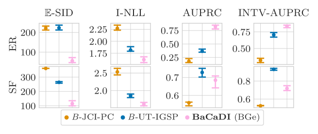
Figure 5: Additional results for Linear Gaussian BNs with $d=20$ nodes. Here, we use the BGe score (Geiger and Heckerman,, 1994, 2002) that marginalizes out the parameters of a linear Gaussian model. We again see how BaCaDI better predicts causal mechanisms across all settings. Note that DCDI-G is not included since it always performs joint inference with parameters.

We again see how BaCaDI outperforms related methods in most metrics, particularly $\mathbb{E}$-SID and I-NLL. Only UT-IGSP performs competitively for AUPRC and INTV-AUPRC of SF graph structures, but fails to be on par with BaCaDI in other settings. These results resonate with the other experimental evaluations, showing promising results for making causal structure predictions.

Appendix D EXPERIMENTAL SETUP

In the following, we describe the models, datasets and implementations that were used to perform experiments in detail. The code is available under https://github.com/haeggee/bacadi.

D.1 Model Details & BaCaDI

First, we discuss the models of graphs as well as the exact usage of BaCaDI .

Graphs. We consider DAGs that follow either Erdős-Rényi  (ER) (Gilbert,, 1959) or scale-free (SF) (Barabási and Albert,, 1999) distributions. ER graphs follow a prior distribution

$$p({\bf{G}})\propto q^{\|{\bf{G}}\|_{1}}(1-q)^{{{d}\choose{2}}-\|{\bf{G}}\|_{1}}$$ (34)

that describes that each edge exists independently w.p. $q$. For SF graphs, we define a prior

$$p({\bf{G}})\propto\prod_{i=1}^{d}(1+\|{\bf{G}}_{i}\|_{1})^{-3}$$ (35)

analogous to their power law degree distribution $p(\text{deg})\sim\text{deg}^{-3}$. ${\bf{G}}_{i}$ describes the $i$-th row of the adjacency matrix. For all our experiments, we use priors that result in $2d$ edges in expectation. Building on Lorch et al., (2021), BaCaDI can incorporate such a graph distribution in the prior $p({\bf{Z}})$ (see Sec. 4.2 in their paper).

Overview: Gaussian BNs. As instantiations of BaCaDI’s inference models that describe the local conditional distributions, we consider Bayesian networks with additive Gaussian noise. This means that the variables ${\mathbf{x}}=({x}_{1},\dots,{x}_{d})$ follow a distribution

$$p({x}_{i}|{\bf{\Theta}},{\bf{G}})=\mathcal{N}(f({x}_{{\text{pa}_{{\bf{G}}}(i)}},{\bf{\Theta}}),\sigma_{i})$$ (36)

For the inference with BaCaDI, we assume a fixed observation noise $\sigma_{i}^{2}=\sigma^{2}=0.1$.

The function $f$ can be modelled in different ways as follows.

Linear BNs. Linear Gaussian BNs model the mean of a given variable as a linear function of its parents:

$$p({\mathbf{x}}|{\bf{\Theta}},{\bf{G}})=\mathcal{N}(({\bf{G}}\circ{\bf{\Theta}})^{T}{\mathbf{x}},\sigma\mathbf{I}),$$ (37)

where $\circ$ denotes the element-wise multiplication. We use this parametrization as it allows for constant dimensionality of ${\bf{\Theta}}\in\mathbb{R}^{d\times d}$ and the elementwise multiplication only keeps the parents of each variable. Moreover, this allows the use of the Gumbel-Softmax estimator in Eq. 18.

As a prior, we use a standard Gaussian $p({\bf{\Theta}}_{i,j}|{\bf{G}}_{i,j}=1)=\mathcal{N}(0,1)$.

Nonlinear BNs. The local conditionals can be extended to nonlinear dependencies modelled by neural networks. We consider feed-forward neural networks of the form

$$\text{FFN}({\mathbf{x}};{\bf{\Theta}}):={\bf{\Theta}}^{(L)}\sigma(\dots,{\bf{\Theta}}^{(1)}{\mathbf{x}}+{\theta}_{b}^{(1)})\dots)+{\theta}_{b}^{(L)},$$ (38)

where ${\bf{\Theta}}=(({\bf{\Theta}}^{(L)},\theta_{b}^{(L)}),\dots,({\bf{\Theta}}^{(1)},\theta_{b}^{(1)}))$ describe the parameters of the $l$-th layer for $l\in\{1,\dots,L\}$. The function $\sigma$ is the element-wise nonlinear activation function and $\theta_{b}^{(l)}$ is the bias. This then gives the distribution

$$p({\mathbf{x}}|{\bf{\Theta}},{\bf{G}})=\prod_{i=1}^{d}\mathcal{N}({x}_{i};\text{FFN}({\bf{G}}_{i}^{T}\circ{\mathbf{x}};{\bf{\Theta}}_{i}),\sigma).$$ (39)

Note that we thus have one neural network defined by ${\bf{\Theta}}_{i}$ for each of the local conditional distributions of variable $i$, that is, $d$ networks in total. For all experiments, we use one hidden layer with $5$ units and the sigmoid activation function.

As a prior for the parameters, we analogously use a standard Gaussian with mean 0 and variance 1.

Interventions. We model interventions using a Gaussian likelihood $p_{i}^{I_{k}}({x}_{i}|{\bf{\Theta}}_{I_{k}})=\mathcal{N}(x_{i}|\mu^{I}_{k,i},\sigma_{I})$ with fixed variance ${\sigma_{I}}^{2}=0.5$. We infer the means ${\bf{\Theta}}_{I_{k}}=[\mu^{I}_{k,1},...,\mu^{I}_{k,d}]$ for which we set a wide Gaussian prior $p({\bf{\Theta}}_{I_{k}}|I^{\text{tar}}_{k})=\prod_{i\in I^{\text{tar}}_{k}}p(\mu^{I}_{k,i}|I^{\text{tar}}_{k,i}=1)=\prod_{i\in I^{\text{tar}}_{k}}\mathcal{N}(\mu^{I}_{k,i}|0,10)$. This reflects an uninformative prior over a large effect range of the interventions.

Initialization. For the linear Gaussians, the parameters are initialized closed to zero via ${\bf{\Theta}}_{\text{init}}\sim\mathcal{N}(0,\sigma_{\text{init}}\mathbf{I})$ with $\sigma_{\text{init}}=0.3$. The closeness to zero is important to avoid inducing a bias at the start of the SVGD inference process. Similarly, we sample ${\bf{\Theta}}_{\mathcal{I},\text{init}}\sim\mathcal{N}(0,\sigma_{\mathcal{I},\text{init}}\mathbf{I})$ with $\sigma_{\mathcal{I},\text{init}}^{2}=0.1$.

For nonlinear Gaussians, we use the Glorot (sometimes called Xavier) normal to initialize the weights of the neural networks. (Glorot and Bengio,, 2010).

SVGD. We instantiate BaCaDI with the SVGD algorithm as discussed in Sec. 6 and shown in Alg. 1. In all our experiments, we use 20 particles, which matches the number of bootstrap samples for the baselines (see D.4).

D.2 Data Generation for the Synthetic Causal Inference Tasks

The data generation is done as follows: we first sample a random graph (either ER or SF) and then sample random parameters. We collect data samples by iterating through the topological ordering of the graph and sample a variable given its local parents. Since we consider additive Gaussian models, each variable is described by a distribution of the form ${x}_{i}|{\bf{\Theta}},{\bf{G}}\sim\mathcal{N}(f({x}_{{\text{pa}_{{\bf{G}}}(i)}},{\bf{\Theta}}),\sigma_{i})$ where $f$ is either a linear function or a nonlinear feedforward neural network (cf. Sec. D.1). The noise variables $\sigma_{i}$ are sampled per variable and fixed once from $\sigma_{i}^{2}\sim\mathcal{U}[0.05,0.15]$. If the noise variables had the same variance across all variables in the graph, this would render identification possible (Peters and Bühlmann,, 2014).

Parameters. The parameters and generative models are initialized as follows:

• Linear BNs: We sample the parameters ${\bf{\Theta}}$ uniformly and independently from $\mathcal{U}([-2,-0.5]\cup[0.5,2])$ in order to bound the weights sufficiently away from zero.

• Nonlinear BNs: The NNs for each local conditional are the same model as used for BaCaDI as well as DCDI-G, that is, a fully connected NN with single hidden layer of size of $5$ with biases. The nonlinear activations are sigmoid functions. All weights and biases are drawn randomly and independently from a Gaussian $\mathcal{N}(0,1)$.

Interventions. As described in the main text, we perform hard interventions on every node for the $20$-node graphs. We create random values by first sampling $\hat{\mu}_{k,i}\sim\mathcal{N}(0,2)$ and then setting ${\mu}_{k,i}^{I}=\text{sign}(\hat{\mu}_{k,i})\cdot 5+\hat{\mu}_{k,i}$. This ensures that the interventions performed are bounded away from zero and out-of-distribution. If a variable $x_{i}$ is the target of the intervention in context $k$, we then have $p_{i}^{I_{k}}({x}_{i}|{\bf{\Theta}}_{I_{k}})=p_{i}^{I_{k}}({x}_{i}|{\mu}_{k,i}^{I})=\mathcal{N}(x_{i};\mu_{k,i}^{I},\sigma_{I})$, where $\sigma_{I}^{2}=0.5$.

D.3 Data Generation with the SERGIO Gene-Expression Simulator

SERGIO (Dibaeinia and Sinha,, 2020) is a single-cell expression simulator for gene regulatory networks (GRNs). The software tool can generate realistic single-cell transcriptomics datasets based on a user-defined graph input that describes the regulatory network. SERGIO uses stochastic differential equations to simulate a gene’s expression dynamics as a function of the changing levels of its regulators. The simulations resemble the data collected by modern high-throughput, single-cell RNA sequencing (scRNA-seq) technologies and are thus more practically-relevant than simulators approximating “bulk” microarray data (Schaffter et al.,, 2011). For more details, we refer to the original paper by Dibaeinia and Sinha, (2020). In the following, we give a brief overview of how we simulate scRNA-seq data with SERGIO. For this, we use an implementation that is adapted from the open-source code available under https://github.com/PayamDiba/SERGIO, which is published under a GPL-3.0 license.

Simulation. SERGIO generates synthetic scRNA-seq data $\mathbf{D}$ for a given causal graph with $d$ genes by first simulating clean gene expression data and then corrupting these expressions with technical measurement noise. The $N$ observations in $\mathbf{D}$ correspond to $N$ cell samples, i.e. one row in $\mathbf{D}$ describes the joint expression of the $d$ genes in a single cell. For simplicity, we do not add the technical noise modules in our experiments.

To simulate the single-cell gene expressions, SERGIO samples randomly-timed expression snapshots from the steady state of the stochastic dynamical system modeling the GRN. In this regulatory process, the genes are expressed at rates influenced by other genes using the chemical Langevin equation. The source nodes in the causal graph ${\bf{G}}$ are denoted master regulators (MRs), whose expressions evolve at constant production and decay rates. The downstream gene expressions evolve non-linearly under production rates caused by the expression of their causal parents in ${\bf{G}}$. To model different cell types, SERGIO varies the specifications of the MR production rates, which significantly influence the evolution of the system. As a result, the data contains variation across cell types and due to biological noise within cells of the same type. In our experiments, we generate single-cell samples collected from ten cell types (Dibaeinia and Sinha,, 2020).

Interventions. We consider knockout interventions that clip the expression of a specific gene to zero. To this end, we extend SERGIO by forcing the production rate of knocked-out genes to be zero during simulation. As described in the main text, we do this for $M=10$ gene targets and arrive at $11$ contexts, including the observational setting.

Parameters. To specify the simulation parameters of SERGIO, we follow the settings suggested by Dibaeinia and Sinha, (2020) for synthetic data generation. Given a causal graph ${\bf{G}}$, the simulation for $c$ cell types of $d$ genes is governed by the following parameters:

• $k\in\mathbb{R}^{d\times d},k_{i,j}\sim\mathcal{U}[1,5]$ : interaction strength if edge $i\rightarrow j$ exists in ${\bf{G}}$

• $b\in\mathbb{R}_{+}^{d\times c},b_{i,j}\sim\mathcal{U}[1,3]:$ MR production rates if $j$ is a source node in ${\bf{G}}$

• $\gamma\in\mathbb{R}_{+}^{d\times d},\gamma_{i,j}=2$ : Hill function coefficients controlling nonlinearity of interactions

• $\lambda\in\mathbb{R}^{d},\lambda_{i}=0.8$ : decay rates per gene

• $\zeta\in\mathbb{R}_{+}^{d},\zeta_{i}=1.0$ : scale of stochastic process noise in chemical Langevin equation

We standardize the data for all methods by subtracting the empirical mean and dividing by the standard deviation.

D.4 Baselines & Implementation

In this section, we provide additional details on the baseline methods and their implementations used in our experiments.

For all methods, we use implementations adapted from the source code of DCDI available under https://github.com/slachapelle/dcdi (where the authors also included their baselines’ code). The implementation of JCI-PC is a modified version of the R package using code from the JCI repository https://github.com/caus-am/jci/tree/master/jci. UT-IGSP has an implementation available from https://github.com/uhlerlab/causaldag.

DAG Bootstrap. To compare all methods in Bayesian model averaging, we employ the nonparametric DAG bootstrap (Friedman et al.,, 1999). It performs model averaging by bootstrapping the observations $\mathbf{D}$ to yield a collection of synthetic data sets, each of which is used to learn a single graph. We sample with replacement from $\mathbf{D}$ for each dataset $\mathcal{D}_{k}$ individually. The collection of unique single graphs approximates the posterior by weighting each graph by its unnormalized posterior probability.

All of the methods are evaluated with 20 bootstrap samples, i.e. the same number of samples as particles used for the SVGD instantiation of BaCaDI. For DCDI-G, we only use 5 bootstrap samples due to the significantly longer runtimes.

JCI-PC. The Joint Causal Inference (JCI) framework (Mooij et al.,, 2016) introduces a general formulation to extend the initial causal graph by auxiliary nodes that describe the different contexts, effectively performing causal discovery over a graph of size $d+M$. This approach can be instiantiated with different standard algorithms. In our experiments, we use the PC algorithm (Spirtes et al.,, 2000), which relies on conditional independence tests (CI) to discover the Markov Equivalence Class (MEC), i.e. the skeleton of a graph with v-structures as well as possible identifiable edge directions. The PC algorithm uses a Gaussian CI test with significance threshold $\alpha^{\text{JCI}}$, which are best-suited for Gaussian BNs.

For computing the graph metrics, we compute the $\mathbb{E}$-SID between the CPDAGs of the GT graph and predictions of JCI-PC. Additionally, we favor JCI-PC when computing AUPRC scores. See Sec. D.5 for more details.

To arrive at a DAG that we can use to estimate MLE parameters and compute log-likelihood metrics, we generate a random consistent expansion of the CPDAG as defined by Chickering, (2002) using the algorithm by Dor and Tarsi, (1992). That is, we generate a DAG s.t. the CPDAG has the same skeleton and v-structures and every directed edge in the CPDAG has the same direction in the DAG.

UT-IGSP. The interventional greedy sparsest permutation (IGSP) method (Wang et al.,, 2017; Yang et al.,, 2018) proposes an algorithm that learns causal structures via local scores based on CI relations and permutation search. The work is extended by Squires et al., (2020) to the case of unknown targets (UT-IGSP). Analogous to JCI-PC, IGSP uses Gaussian CI and invariance tests with parameters $\alpha^{\text{UT-IGSP}}$ and $\alpha^{\text{UT-IGSP}}_{\text{inv}}$. Since we study the low sample setting, it is possible that the algorithm as provided by their open source implementation fails to compute an essential correlation matrix. Specifically, the algorithm computes a correlation matrix that becomes singular in the case when the number of unique samples is smaller than the number of variables considered, thus rendering an inversion of this matrix impossible. In case this happens, we retry the inference with a halved $\alpha^{\text{UT-IGSP}}$ confidence threshold. The maximum number of restarts is set to $10$, and the bootstrap sample is dropped in case this maximum is reached.

Similar to JCI-PC, the $\mathbb{E}$-SID is computed as the midpoint of the lower and upper bound between the CPDAGs of the GT graph and predictions of UT-IGSP. As for JCI-PC, we favor UT-IGSP when computing AUPRC scores. See Sec. D.5 for more details. Likewise, we obtain a DAG by generating a random consistent expansion of the CPDAG to compute the log-likelihood metrics.

DCDI-G. Brouillard et al., (2020) introduced Differentiable Causal Discovery from Interventional Data (DCDI), which performs causal structure learning via the augmented Lagrangian method. The algorithm formulates a continuous-constrained optimization problem that relies on stochastic gradient descent and neural networks to fit the local conditionals.

To ensure a fair comparison, we employ the exact same likelihood model as used for the nonlinear Gaussian BNs used in BaCaDI, that is, a feedforward neural network with one hidden layer of size $5$ and Gaussian additive noise. This model is called DCDI-G in (Brouillard et al.,, 2020). However, we use a smaller neural network to model the means of the local conditional distributions than originally used by Brouillard et al., (2020). In initial experiments with DCDI-G, we observed strong overfitting due to our low-sample regime and thus reduced the model capacity. As suggested by Brouillard et al., (2020), we use the leaky ReLU with negative slope of $0.25$ as elementwise activation function. To obtain comparable log-likelihood metrics, we fix the noise variables to $\sigma^{2}=0.1$ as done for BaCaDI. These noise variables could generally be learned by both methods.

D.5 Metrics

Our reported metrics focus on three essential aspects of our inference problem: causal graph prediction, intervention detection, and learning the local conditional distributions of the individual variables.

• SID: The Structural Interventional Distance (SID) (Peters and Bühlmann,, 2015) quantifies the closeness between two DAGs in terms of how well their interventional adjustment sets coincide. Since we perform posterior inference and arrive at a distribution over graphs, we consider the expected SID, which is defined as

  $$\mathbb{E}\text{-SID}(p,{\bf{G}}_{\text{gt}}):=\sum_{{\bf{G}}}p({\bf{G}}|\mathcal{D})\cdot\text{SID}({\bf{G}},{\bf{G}}_{\text{gt}})$$ (40)

  To compute the SID, we use the implementation provided by the Causal Discovery Toolbox (Kalainathan and Goudet,, 2019). Since UT-IGSP and JCI-PC only return a CPDAG of the Interventional Markov Equivalence Class (I-MEC), we calculate the lower and upper bound of the SIDs in the I-MEC and report their midpoint as the $\mathbb{E}$-SID. The DAG bootstrap variants for all baselines as well as BaCaDI use the weighted mixture rather than the empirical distribution of samples. The weight is based on the unnormalized log-likelihood achieved on the bootstrap sample.

• SHD: The structural hamming distance (SHD) reflects the graph edit distance to the ground truth DAG. However, it often does not properly reflect the closeness of two DAGs in terms of their causal interpretation. For instance, the trivial prediction of the empty graph achieves competitive SHD scores for the sparse graphs we consider in this paper. In our main text, we thus focus on the $\mathbb{E}$-SID as well as other metrics that together better assess the quality of causal graph predictions. For completeness, we report the $\mathbb{E}$-SHD results in Appx. E.4.

• Threshold metrics: Treating the edge prediction as a classification task, we compute the area under the precision recall curve (AUPRC) for pairwise edge prediction based on the posterior marginals $p(g_{ij}=1|\mathbf{D})$. This marginal is defined as the posterior mean of an indicator variable for the presence of the edge: $p(g_{ij}=1|\mathbf{D})=\mathbb{E}_{p({\bf{G}}|\mathbf{D})}\mathbf{1}[g_{ij}=1]$. The AUPRC provides more insight into predictive performance than, e.g., the AUROC because sparse graphs translate to highly imbalanced edge classification tasks.

  For JCI-PC and UT-IGSP, which both return a CPDAG with edges that are undecided, we favor the methods when computing the AUPRC metric. Specifically, we orient a predicted undirected edge correctly when a ground truth edge exists and only count a falsely predicted undirected edge as a single mistake.

• Interventional AUPRC: Similarly, we report the interventional AUPRC (INTV-AUPRC) for the classification of intervention targets. The INTV-AUPRC captures how well an algorithm predicts which variables have been intervened on. Since we assume sparse interventions, this metric better captures a model’s performance for the imbalanced classification task.

• I-NLL: We compute the average negative interventional log-likelihood (I-LL) on $M^{\text{test}}=10$ heldout interventional datasets $\mathbf{D}^{\text{test}}=\{\mathcal{D}^{\text{test}}_{1},...,\mathcal{D}^{\text{test}}_{10}\}$, where different interventions are performed compared to the training datasets. Each interventional test dataset comprises 100 samples and has known intervention targets $I^{\text{tar}}_{\text{test},k}$ and effect distributions $p(x_{i}|{\bf{\Theta}}_{I_{\text{test},k}})$

  The I-NLL is computed via

  $$\text{I-NLL}(p,\mathbf{D}^{\text{test}}):=-\frac{1}{M^{\text{test}}}\sum_{k=1}^{M^{\text{test}}}\mathbb{E}_{p({\bf{G}},{\bf{\Theta}}|\mathbf{D})}\left[\frac{1}{|\mathcal{D}^{\text{test}}_{k}|}\log p(\mathcal{D}^{\text{test}}_{k}|{\bf{G}},{\bf{\Theta}},I^{\text{tar}}_{\text{test},k},{\bf{\Theta}}_{I_{\text{test},k}})\right]\;.$$

  Since UT-IGSP and JCI-PC are not equipped with local conditional distributions, we use the linear Gaussian maximum-likelihood parameters (MLE), which can be computed in closed-form (Hauser and Bühlmann,, 2014). For the nonlinear datasets, this creates a model mismatch since the closed form is only available for linear Gaussian BNs.

D.6 Hyperparameter Search

To ensure a fair comparison, we perform a hyperparameter search for all baselines. The search ranges can be found in Table 1. Throughout all experiments, we use at least 20 hyperparameter samples and aggregate results over 30 different random seeds and graphs. For the results of BaCaDI in the main text, we fix the hyperparameters $\alpha=0.01$, $\beta=2$ and $\lambda=1$, which are the linear scale for the temperature parameter of the sigmoids, the linear scale for the sparsity regularizer and the sparse intervention regularizer, respectively.

Method	Hyperparameter	Comment	Search range
BaCaDI	$\tau_{Z}$	Kernel lengthscale	$\log_{10}\mathcal{U}[-1,1.7]$
	$\tau_{\gamma}$	Kernel lengthscale	$\log_{10}\mathcal{U}[-1,1.7]$
	$\tau_{\theta}$	Kernel lengthscale	$\log_{10}\mathcal{U}[1.2,5]$
JCI-PC	$\alpha^{\text{JCI}}$	CI tests	$\log_{10}\mathcal{U}[-5,-1]$
UT-IGSP	$\alpha^{\text{UT-IGSP}}$	CI tests	$\log_{10}\mathcal{U}[-5,-1]$
	$\alpha^{\text{UT-IGSP}}_{\text{inv}}$	Invariance tests	$\log_{10}\mathcal{U}[-5,-1]$
DCDI-G	batch size	-	$\mathcal{U}(\{16,32,64\})$
	$\lambda_{R}$	Sparsity coefficient for interventions	$\log_{10}\mathcal{U}[-8,-1]$
	$\lambda$	Sparsity coefficient for graph	$\log_{10}\mathcal{U}[-3,-1]$
	$h$	Convergence threshold	$\log_{10}\mathcal{U}[-8,-6]$

Table 1: Hyperparameter search space for all methods

Appendix E ADDITIONAL EXPERIMENTS

E.1 Larger datasets

We report additional results when doubling the dataset size, i.e. we collect $n_{0}=200$ observational samples and $n_{k}=20$ samples per interventional context. The results for synthetic linear and nonlinear Gaussian BNs can be found in Fig. 6 and Fig. 7, respectively.

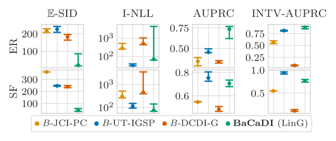
Figure 6: Linear Gaussian with more data. Joint posterior inference over CBNs and interventions for linear Gaussian ground-truth CBNs. The results are for data from ER-2 (top) and SF-2 (bottom) graphs with $d=20$ variables and $M=20$ contexts. Here, we double the dataset size to $N=600$ samples in total. Similar to the previous setting with lower sample sizes, BaCaDI is consistently the most competitive method.

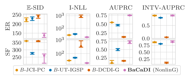
Figure 7: Nonlinear Gaussian with more data. Joint posterior inference over CBNs and interventions for nonlinear Gaussian ground-truth CBNs. The results are for data from ER-2 (top) and SF-2 (bottom) graphs with $d=20$ variables and $M=20$ contexts. Here, we double the dataset size to $N=600$ samples in total. BaCaDI performs the best across all metrics.

E.2 Observational vs. Interventional Data

As an additional interesting use case, we evaluate how interventional data helps predicting the causal structure with BaCaDI. In general, intervening on variables in the system and observing the outcome provides information that helps discovering the causal mechanisms. In the perfect setting, when the intervention targets are fully known, they increase identifiability by shrinking the interventional Markov equivalence class (Hauser and Bühlmann,, 2012). However, the information gain can be limited when the intervention targets are unknown (Squires et al.,, 2020).

We investigate how BaCaDI can leverage such unknown interventions compared to using just observational data. To that end, we evaluate 3 different settings: i) when only observational data is available, ii) interventional data with full knowledge of the interventions, and iii) unknown interventions. When the interventions are known, the posterior inference of BaCaDI can be reduced to Eq. 3.

We consider nonlinear Gaussian BNs for $d=20$ node graphs. All methods receive the exact same number of samples for inference. That is, we collect $n_{0}=300$ samples from the ground-truth BN without interventions for the observational dataset. As before, the interventional datasets have $n_{0}=100$ observations and $n_{k}=10$ samples per interventional context. We report the results in Fig. 8.

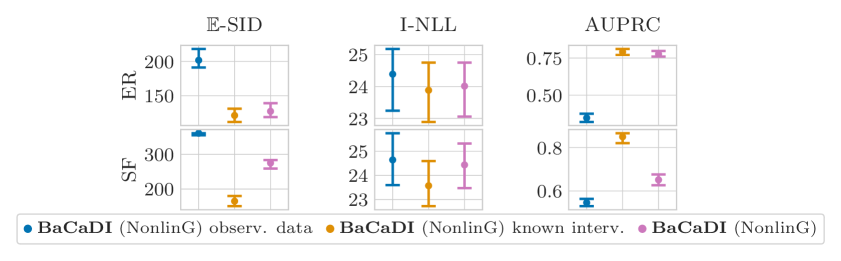
Figure 8: Comparison: Observational data vs. known and unknown interventions. Additional results comparing BaCaDI with observational data against known and unknown interventions for nonlinear Gaussian BNs for $d=20$ node graphs. As a natural baseline, the setting of knowing the intervention targets and effects leads to the best performance across all metrics. When the interventions are unknown, BaCaDI achieves results close to this baseline. Notably, it outperforms the setting where just observational data is available.

We observe that BaCaDI achieves significantly better results when interventional data is available. The case of known interventions serves as a natural baseline, where BaCaDI achieves the best performance and gets closest in recovering the true causal structure. This is most clearly shown by the $\mathbb{E}$-SID and AUPRC scores. Notably, BaCaDI is able to get close this baseline even when interventions are unknown and outperforms the setting where just observational data is available. This shows the benefit of performing and collecting interventions even when some of the effects may be unknown and is a promising result for future work.

E.3 50 Node graphs

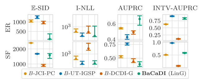
Figure 9: Linear Gaussian BNs with 50 nodes. Additional results comparing BaCaDI on larger graphs with $d=50$ nodes for Linear Gaussian BNs for ER-2 (top) and SF-2 (bottom). BaCaDI performs competitively across all metrics. In particular, it makes significantly better causal mechanism predictions for ER graph as captured by the $\mathbb{E}$-SID.

As additional experiments, we perform posterior inference for larger graphs with $50$ nodes in total. Analogous to the previous evaluations, we consider synthetic linear Gaussian BNs with hard interventions on every node. We use a larger dataset of $n_{0}=200$ observational samples and $n_{k}=20$ samples per interventional context. The results are given in Fig. 9. We find that BaCaDI scales to larger graphs and performs competitively across all metrics. In particular, our method outperforms the baselines by a large margin in terms of the $\mathbb{E}$-SID and AUPRC for ER graphs.

E.4 Structural Hamming Distance

For completeness, we include the Expected Structural Hamming Distance ($\mathbb{E}$-SHD) metric for all results discussed in the main text for $d=20$ node graphs in Table 2. Analogous to the $\mathbb{E}$-SID, the $\mathbb{E}$-SHD is defined as $\mathbb{E}\text{-SHD}(p,{\bf{G}}_{\text{gt}}):=\sum_{{\bf{G}}}p({\bf{G}}|\mathcal{D})\cdot\text{SHD}({\bf{G}},{\bf{G}}_{\text{gt}})$. The SHD reflects the graph edit distance where wrongly inverted edges are counted as only one error. However, while it captures closeness to the ground truth graph, trivial predictions like the empty graph achieve competitive results for sparse graphs. For example, in the setting of $d=20$ nodes and $2d$ edges in expectation, the empty graph will achieve a $\mathbb{E}$-SHD of $40$ in expectation. Similar conclusions hold if only very few edges are predicted. In the main text, we thus resort to the $\mathbb{E}$-SID as well as additional metrics that together report an accurate description of the quality of inference.

	JCI-PC	UT-IGSP	DCDI-G	BaCaDI  (LinG)	BaCaDI  (NonlinG)
Linear Gaussian BNs graphs:
ER-2	38.97 ($1.65$)	41.38 ($2.53$)	63.29 ($4.52$)	50.32 ($10.98$)	-
SF-2	37.42 ($0.32$)	34.35 ($1.18$)	51.68 ($3.67$)	36.48 ($6.12$)	-
Nonlinear Gaussian BNs graphs:
ER-2	38.93 ($1.65$)	35.09 ($1.76$)	64.91 ($2.61$)	-	18.73 ($1.85$)
SF-2	37.00 ($0.00$)	33.75 ($0.48$)	57.92 ($2.69$)	-	23.55 ($1.43$)
SERGIO graphs
SF-2	44.29 ($0.70$)	45.05 ($1.88$)	56.39 ($1.63$)	108.71 ($3.75$)	115.04 ($6.22$)

Table 2: Expected Structural Hamming Distance. We report the $\mathbb{E}$-SHD for all methods for the main results with $d=20$ node graphs. We aggregate results over 30 different seeds and report the mean and standard error. While the $\mathbb{E}$-SHD is a simple and commonly used metric, it can be misleading. For sparse graphs, the trivial prediction of the empty graph achieves competitive $\mathbb{E}$-SHD scores; similar assessments can be made for predictions with only a few edges. We include the results for completeness.

E.5 Runtimes

We report the average runtimes (in minutes) for all methods and main results for $d=20$ node graphs in Table 3.

	JCI-PC	UT-IGSP	DCDI-G	BaCaDI  (LinG)	BaCaDI  (NonlinG)
Linear Gaussian BNs graphs:
ER	2.07$\pm$ 0.16	1.31$\pm$ 0.22	260.03$\pm$56.11	51.68$\pm$13.12	-
SF-2	2.17$\pm$ 0.15	1.46$\pm$ 0.09	176.89$\pm$30.46	60.57$\pm$22.95	-
Nonlinear Gaussian BNs graphs:
ER	1.89$\pm$ 0.07	1.16$\pm$ 0.06	143.88$\pm$12.53	-	491.26$\pm$91.74
SF-2	1.92$\pm$ 0.06	1.41$\pm$ 0.06	145.43$\pm$25.83	-	519.79$\pm$97.95
SERGIO graphs
SF-2	2.36$\pm$ 0.09	0.42$\pm$ 0.20	128.04$\pm$ 9.97	45.11$\pm$ 1.52	323.11$\pm$101.15

Table 3: Average runtimes for all methods for the main results with $d=20$ node graphs. We aggregate results over 30 different seeds and report the mean and standard deviation. All numbers given are in minutes.

E.6 Computational Resources

All experiments reported in this paper were performed in bulk and in parallel on 2-core CPU nodes of an internal cluster. No GPUs were used. We estimate the total compute to amount to roughly 40,000 hours of CPU time.

Appendix F STEIN VARIATIONAL GRADIENT DESCENT

We here give an overview of Stein Variational Gradient Descent (SVGD) introduced by Liu and Wang, (2016). Fundamentally, the work of Liu and Wang, (2016) connects the mathematical notions of probability discrepancies with a variational inference method, which closely resembles the gradient descent algorithm. For details, we refer to the original paper.

Stein’s identity and discrepancy

Formally, let $p({\mathbf{x}})$ be a continuously differentiable (i.e. smooth) density supported on $\mathcal{X}\subseteq\mathbb{R}^{d}$. For a smooth vector function $\phi({\mathbf{x}})$, Stein’s identity states that for sufficiently regular $\phi$, we have

$$\mathbb{E}_{{\mathbf{x}}\sim p}[\mathcal{A}_{p}\phi({\mathbf{x}})]=0,\text{ where } \mathcal{A}_{p}\phi({\mathbf{x}})=\phi({\mathbf{x}})\nabla_{x}\log p({\mathbf{x}})^{T}+\nabla_{x}\phi({\mathbf{x}})$$ (41)

where $\mathcal{A}_{p}$ is the Stein operator acting on the function $\phi$. This equation can be subsequently used as a discrepancy measure: when considering the expectation over a smooth density $q$ different than $p$, we obtain the so called Stein discrepancy by considering the maximum violation of Stein’s identity. That is, we have

$$\mathbb{S}(q,p)=\max_{\phi\in\mathcal{F}}[\mathbb{E}_{{\mathbf{x}}\sim q}[\text{trace}(\mathcal{A}_{p}\phi({\mathbf{x}}))]^{2}]$$ (42)

for a choice of a set of functions $\mathcal{F}$, for instance the reproducing kernel Hilbert space (RKHS) denoted by $\mathcal{H}^{d}$.

Variational Inference using smooth transforms

The goal of variational inference is to approximate a target distribution $p$ using a simpler distribution $q^{*}$ which minimizes the KL-divergence

$$q^{*}=\operatorname*{arg\,min}_{q\in\mathcal{Q}}KL(q||p)$$ (43)

In order to minimize the KL-divergence, the authors in (Liu and Wang,, 2016) consider incremental transforms formed by a small perturbation to the identity map that make up the set of distributions $\mathcal{Q}$. That is, the transform $\mathbf{T}:\mathcal{X}\rightarrow\mathcal{X}$ is defined as

$$\mathbf{T}({\mathbf{x}})={\mathbf{x}}+\epsilon\phi({\mathbf{x}})$$ (44)

where $\phi$ is a smooth function that characterizes the perturbation direction. As a key result, Liu and Wang, (2016) connect these transforms to the Stein operator and the derivative of the KL divergence. The authors show that if the function $\phi$ lies in the ball of the vector valued RKHS $\mathcal{H}^{d}$, the direction of the steepest descent on the KL divergence between a fixed $q$ and the target $p$ is given by

$$\phi_{q,p}^{*}=\mathbb{E}_{{\mathbf{x}}\sim q}[k({\mathbf{x}},\cdot)\nabla_{{\mathbf{x}}}\log p({\mathbf{x}})+\nabla_{{\mathbf{x}}}k({\mathbf{x}},\cdot)]$$ (45)

where one can easily identify the form of the Stein operator. What is more, the value of the obtained gradient equals the (negative) kernelized Stein discrepancy measure $-\mathbb{S}(q,p)$.

General Algorithm

This mathematical result suggests an iterative method that transforms an initial reference distribution $q_{0}$ to the target distribution $p$. Starting with a finite set of random particles $\{{\mathbf{x}}^{(m)}\}_{m=1}^{M}$, for some iteration $t$ each particle is updated deterministically according to

$${\mathbf{x}}_{t+1}^{(m)}\leftarrow{\mathbf{x}}_{t}^{(m)}+\epsilon_{t}\phi({\mathbf{x}}_{t+1}^{(m)})$$ (46)

$$\text{ where }\phi({\mathbf{x}})=\frac{1}{M}\sum_{l=1}^{M}k({\mathbf{x}}_{t+1}^{(l)},{\mathbf{x}})\nabla_{{\mathbf{x}}}\log p({\mathbf{x}})+\nabla_{{\mathbf{x}}}k({\mathbf{x}}_{t+1}^{(l)},{\mathbf{x}})$$ (47)

These steps iteratively decrease the KL divergence between $q_{t}$ and $p$, ultimately converging.

Importantly, the advantage of SVGD is that it only depends on the gradient of the kernel $k(x,\cdot)$ that can be defined for the application, as well as the score function $\nabla_{{\mathbf{x}}}\log p(x)$ which can be computed without knowing the (intractable) normalization constant of $p$. On an intuitive level, the first part of the perturbation direction expression drives the particles to high density regions close to the mode of the target distribution $p$, whereas the term $\nabla_{{\mathbf{x}}}k({\mathbf{x}},\cdot)$ acts as a repulsive force that prevents the particles from collapsing together.

References

- Agrawal et al., (2019) Agrawal, R., Squires, C., Yang, K., Shanmugam, K., and Uhler, C. (2019). ABCD-Strategy: Budgeted experimental design for targeted causal structure discovery. In Proceedings of Machine Learning Research, volume 89, pages 3400–3409. PMLR.
- Albert, (2005) Albert, R. (2005). Scale-free networks in cell biology. Journal of cell science, 118(21):4947–4957.
- Annadani et al., (2021) Annadani, Y., Rothfuss, J., Lacoste, A., Scherrer, N., Goyal, A., Bengio, Y., and Bauer, S. (2021). Variational causal networks: Approximate bayesian inference over causal structures. arXiv preprint arXiv:2106.07635.
- Barabási and Albert, (1999) Barabási, A.-L. and Albert, R. (1999). Emergence of scaling in random networks. Science, 286(5439):509–512.
- Blei et al., (2017) Blei, D. M., Kucukelbir, A., and McAuliffe, J. D. (2017). Variational inference: A review for statisticians. Journal of the American Statistical Association, 112(518):859–877.
- Brouillard et al., (2020) Brouillard, P., Lachapelle, S., Lacoste, A., Lacoste-Julien, S., and Drouin, A. (2020). Differentiable causal discovery from interventional data.
- Chen et al., (2014) Chen, T., Fox, E., and Guestrin, C. (2014). Stochastic Gradient Hamiltonian Monte Carlo. In International Conference on Machine Learning, pages 1683–1691. PMLR.
- Chickering, (2002) Chickering, D. M. (2002). Optimal structure identification with greedy search. Journal of Machine Learning Research, 3(Nov):507–554.
- Cho et al., (2016) Cho, H., Berger, B., and Peng, J. (2016). Reconstructing causal biological networks through active learning. PloS one, 11(3):e0150611.
- Cundy et al., (2021) Cundy, C., Grover, A., and Ermon, S. (2021). Bcd nets: Scalable variational approaches for bayesian causal discovery. Advances in Neural Information Processing Systems, 34:7095–7110.
- Dibaeinia and Sinha, (2020) Dibaeinia, P. and Sinha, S. (2020). SERGIO: a single-cell expression simulator guided by gene regulatory networks. Cell systems, 11(3):252–271.
- Dor and Tarsi, (1992) Dor, D. and Tarsi, M. (1992). A simple algorithm to construct a consistent extension of a partially oriented graph. Technicial Report R-185, Cognitive Systems Laboratory, UCLA.
- Eaton and Murphy, (2007) Eaton, D. and Murphy, K. (2007). Exact bayesian structure learning from uncertain interventions. In Artificial intelligence and statistics, pages 107–114. PMLR.
- Eberhardt et al., (2005) Eberhardt, F., Glymour, C., and Scheines, R. (2005). On the number of experiments sufficient and in the worst case necessary to identify all causal relations among n variables. In Proceedings of the 21st Conference on Uncertainty in Artificial Intelligence.
- Eberhardt et al., (2006) Eberhardt, F., Glymour, C., and Scheines, R. (2006). N-1 experiments suffice to determine the causal relations among n variables. In Innovations in machine learning, pages 97–112. Springer.
- Faria et al., (2022) Faria, G. R., Martins, A. F., and Figueiredo, M. A. (2022). Differentiable causal discovery under latent interventions. arXiv preprint arXiv:2203.02336.
- Friedman et al., (1999) Friedman, N., Goldszmidt, M., and Wyner, A. (1999). Data analysis with bayesian networks: A bootstrap approach. page 196–205.
- Friedman and Koller, (2003) Friedman, N. and Koller, D. (2003). Being Bayesian About Network Structure. A Bayesian Approach to Structure Discovery in Bayesian Networks. Machine Learning, 50(1):95–125.
- Geiger and Heckerman, (1994) Geiger, D. and Heckerman, D. (1994). Learning gaussian networks. In Uncertainty Proceedings 1994, pages 235–243. Elsevier.
- Geiger and Heckerman, (2002) Geiger, D. and Heckerman, D. (2002). Parameter priors for directed acyclic graphical models and the characterization of several probability distributions. The Annals of Statistics, 30(5):1412–1440.
- Ghassami et al., (2017) Ghassami, A., Salehkaleybar, S., Kiyavash, N., and Zhang, K. (2017). Learning causal structures using regression invariance. Advances in Neural Information Processing Systems, 30.
- Gilbert, (1959) Gilbert, E. N. (1959). Random graphs. The Annals of Mathematical Statistics, 30(4):1141–1144.
- Glorot and Bengio, (2010) Glorot, X. and Bengio, Y. (2010). Understanding the difficulty of training deep feedforward neural networks. In Proceedings of the thirteenth international conference on artificial intelligence and statistics, pages 249–256. JMLR Workshop and Conference Proceedings.
- Grzegorczyk, (2010) Grzegorczyk, M. (2010). An introduction to Gaussian Bayesian networks. In Systems Biology in Drug Discovery and Development, pages 121–147. Springer.
- Hauser and Bühlmann, (2012) Hauser, A. and Bühlmann, P. (2012). Characterization and Greedy Learning of Interventional Markov Equivalence Classes of Directed Acyclic Graphs.
- Hauser and Bühlmann, (2014) Hauser, A. and Bühlmann, P. (2014). Jointly interventional and observational data: estimation of interventional markov equivalence classes of directed acyclic graphs. Journal of the Royal Statistical Society: Series B (Statistical Methodology), 77(1):291–318.
- Heinze-Deml et al., (2018) Heinze-Deml, C., Peters, J., and Meinshausen, N. (2018). Invariant causal prediction for nonlinear models. Journal of Causal Inference, 6(2).
- Hoyer et al., (2008) Hoyer, P., Janzing, D., Mooij, J. M., Peters, J., and Schölkopf, B. (2008). Nonlinear causal discovery with additive noise models. Advances in neural information processing systems, 21.
- Huang et al., (2018) Huang, B., Zhang, K., Lin, Y., Schölkopf, B., and Glymour, C. (2018). Generalized score functions for causal discovery. In Proceedings of the 24th ACM SIGKDD International Conference on Knowledge Discovery & Data Mining, pages 1551–1560.
- Huang et al., (2020) Huang, B., Zhang, K., Zhang, J., Ramsey, J., Sanchez-Romero, R., Glymour, C., and Schölkopf, B. (2020). Causal Discovery from Heterogeneous/Nonstationary Data. Journal of Machine Learning Research, 21(89):1–53.
- Hyttinen et al., (2013) Hyttinen, A., Eberhardt, F., and Hoyer, P. O. (2013). Experiment selection for causal discovery. Journal of Machine Learning Research, 14:3041–3071.
- Jaber et al., (2020) Jaber, A., Kocaoglu, M., Shanmugam, K., and Bareinboim, E. (2020). Causal discovery from soft interventions with unknown targets: Characterization and learning. In Larochelle, H., Ranzato, M., Hadsell, R., Balcan, M., and Lin, H., editors, Advances in Neural Information Processing Systems, volume 33, pages 9551–9561. Curran Associates, Inc.
- Jang et al., (2016) Jang, E., Gu, S., and Poole, B. (2016). Categorical reparameterization with gumbel-softmax. arXiv preprint arXiv:1611.01144.
- Kalainathan and Goudet, (2019) Kalainathan, D. and Goudet, O. (2019). Causal discovery toolbox: Uncover causal relationships in python.
- Ke et al., (2019) Ke, N. R., Bilaniuk, O., Goyal, A., Bauer, S., Larochelle, H., Schölkopf, B., Mozer, M. C., Pal, C., and Bengio, Y. (2019). Learning neural causal models from unknown interventions.
- Kuipers and Moffa, (2022) Kuipers, J. and Moffa, G. (2022). The interventional Bayesian Gaussian equivalent score for Bayesian causal inference with unknown soft interventions.
- Kuipers et al., (2014) Kuipers, J., Moffa, G., and Heckerman, D. (2014). Addendum on the scoring of gaussian directed acyclic graphical models. The Annals of Statistics, 42(4):1689–1691.
- Lachapelle et al., (2019) Lachapelle, S., Brouillard, P., Deleu, T., and Lacoste-Julien, S. (2019). Gradient-based neural DAG learning. arXiv preprint arXiv:1906.02226.
- Liu, (2017) Liu, Q. (2017). Stein variational gradient descent as gradient flow. Advances in neural information processing systems, 30.
- Liu and Wang, (2016) Liu, Q. and Wang, D. (2016). Stein variational gradient descent: A general purpose bayesian inference algorithm. In Advances in Neural Information Processing.
- Lorch et al., (2021) Lorch, L., Rothfuss, J., Schölkopf, B., and Krause, A. (2021). DiBS: Differentiable Bayesian Structure Learning. Advances in Neural Information Processing Systems, 34:24111–24123.
- Maddison et al., (2017) Maddison, C. J., Mnih, A., and Teh, Y. W. (2017). The concrete distribution: A continuous relaxation of discrete random variables. In Proceedings International Conference on Learning Representations.
- Madigan et al., (1995) Madigan, D., Gavrin, J., and Raftery, A. E. (1995). Eliciting prior information to enhance the predictive performance of bayesian graphical models. Communications in Statistics-Theory and Methods, 24(9):2271–2292.
- Madigan and Raftery, (1994) Madigan, D. and Raftery, A. E. (1994). Model selection and accounting for model uncertainty in graphical models using occam’s window. Journal of the American Statistical Association, 89(428):1535–1546.
- Magliacane et al., (2016) Magliacane, S., Claassen, T., and Mooij, J. M. (2016). Ancestral causal inference. Advances in Neural Information Processing Systems, 29.
- McFarland et al., (2020) McFarland, J. M., Paolella, B. R., Warren, A., Geiger-Schuller, K., Shibue, T., Rothberg, M., Kuksenko, O., Colgan, W. N., Jones, A., Chambers, E., et al. (2020). Multiplexed single-cell transcriptional response profiling to define cancer vulnerabilities and therapeutic mechanism of action. Nature communications, 11(1):1–15.
- Meinshausen et al., (2016) Meinshausen, N., Hauser, A., Mooij, J. M., Peters, J., Versteeg, P., and Bühlmann, P. (2016). Methods for causal inference from gene perturbation experiments and validation. Proceedings of the National Academy of Sciences, 113(27):7361–7368.
- Mooij et al., (2016) Mooij, J. M., Magliacane, S., and Claassen, T. (2016). Joint Causal Inference from Multiple Contexts.
- Murphy, (2001) Murphy, K. P. (2001). Active learning of causal bayes net structure.
- Ouma et al., (2018) Ouma, W. Z., Pogacar, K., and Grotewold, E. (2018). Topological and statistical analyses of gene regulatory networks reveal unifying yet quantitatively different emergent properties. PLoS computational biology, 14(4):e1006098.
- Pearl, (2009) Pearl, J. (2009). Causality. Cambridge University Press, 2 edition.
- Peters and Bühlmann, (2014) Peters, J. and Bühlmann, P. (2014). Identifiability of Gaussian structural equation models with equal error variances. Biometrika, 101(1):219–228.
- Peters and Bühlmann, (2015) Peters, J. and Bühlmann, P. (2015). Structural intervention distance for evaluating causal graphs. Neural computation, 27(3):771–799.
- Peters et al., (2016) Peters, J., Bühlmann, P., and Meinshausen, N. (2016). Causal inference by using invariant prediction: identification and confidence intervals. Journal of the Royal Statistical Society. Series B (Statistical Methodology), pages 947–1012.
- Peters et al., (2017) Peters, J., Janzing, D., and Schölkopf, B. (2017). Elements of Causal Inference: Foundations and Learning Algorithms. MIT Press, Cambridge, MA, USA.
- Reisach et al., (2021) Reisach, A., Seiler, C., and Weichwald, S. (2021). Beware of the simulated dag! causal discovery benchmarks may be easy to game. Advances in Neural Information Processing Systems, 34:27772–27784.
- Robinson, (1973) Robinson, R. (1973). Counting labeled acyclic digraphs. New Directions in the Theory of Graphs.
- Schaffter et al., (2011) Schaffter, T., Marbach, D., and Floreano, D. (2011). GeneNetWeaver: in silico benchmark generation and performance profiling of network inference methods. Bioinformatics, 27(16):2263–2270.
- Scherrer et al., (2021) Scherrer, N., Bilaniuk, O., Annadani, Y., Goyal, A., Schwab, P., Schölkopf, B., Mozer, M. C., Bengio, Y., Bauer, S., and Ke, N. R. (2021). Learning neural causal models with active interventions. arXiv preprint arXiv:2109.02429.
- Schölkopf et al., (2012) Schölkopf, B., Janzing, D., Peters, J., Sgouritsa, E., Zhang, K., and Mooij, J. M. (2012). On causal and anticausal learning. In Proceedings of the 29th International Conference on Machine Learning (ICML), pages 1255–1262.
- Schölkopf et al., (2021) Schölkopf, B., Locatello, F., Bauer, S., Ke, N. R., Kalchbrenner, N., Goyal, A., and Bengio, Y. (2021). Toward causal representation learning. Proceedings of the IEEE, 109(5):612–634.
- Shimizu et al., (2006) Shimizu, S., Hoyer, P. O., Hyvärinen, A., Kerminen, A., and Jordan, M. (2006). A linear non-gaussian acyclic model for causal discovery. Journal of Machine Learning Research, 7(10).
- Solus et al., (2017) Solus, L., Wang, Y., Matejovicova, L., and Uhler, C. (2017). Consistency guarantees for permutation-based causal inference algorithms. arXiv preprint arXiv:1702.03530.
- Spirtes et al., (2000) Spirtes, P., Glymour, C. N., Scheines, R., and Heckerman, D. (2000). Causation, prediction, and search. MIT press.
- Squires et al., (2020) Squires, C., Wang, Y., and Uhler, C. (2020). Permutation-Based Causal Structure Learning with Unknown Intervention Targets.
- Srivatsan et al., (2020) Srivatsan, S. R., McFaline-Figueroa, J. L., Ramani, V., Saunders, L., Cao, J., Packer, J., Pliner, H. A., Jackson, D. L., Daza, R. M., Christiansen, L., et al. (2020). Massively multiplex chemical transcriptomics at single-cell resolution. Science, 367(6473):45–51.
- Tong and Koller, (2001) Tong, S. and Koller, D. (2001). Active learning for structure in bayesian networks. In International Joint Conference on Artificial Intelligence, volume 17, pages 863–869.
- Wang et al., (2022) Wang, Y., Cao, F., Yu, K., and Liang, J. (2022). Efficient causal structure learning from multiple interventional datasets with unknown targets. Proceedings of the AAAI Conference on Artificial Intelligence, 36(8):8584–8593.
- Wang et al., (2017) Wang, Y., Solus, L., Yang, K., and Uhler, C. (2017). Permutation-based causal inference algorithms with interventions. Advances in Neural Information Processing Systems, 30.
- Welling and Teh, (2011) Welling, M. and Teh, Y. W. (2011). Bayesian Learning via Stochastic Gradient Langevin Dynamics. In International Conference on Machine Learning, page 681–688.
- Yang et al., (2018) Yang, K., Katcoff, A., and Uhler, C. (2018). Characterizing and learning equivalence classes of causal dags under interventions. In International Conference on Machine Learning, pages 5541–5550. PMLR.
- Yu et al., (2019) Yu, Y., Chen, J., Gao, T., and Yu, M. (2019). DAG-GNN: DAG structure learning with graph neural networks. In International Conference on Machine Learning, pages 7154–7163. PMLR.
- Zhang et al., (2017) Zhang, K., Huang, B., Zhang, J., Glymour, C., and Schölkopf, B. (2017). Causal Discovery from Nonstationary/Heterogeneous Data: Skeleton Estimation and Orientation Determination. In Proceedings of the Twenty-Sixth International Joint Conference on Artificial Intelligence, IJCAI-17, pages 1347–1353.
- Zheng et al., (2018) Zheng, X., Aragam, B., Ravikumar, P., and Xing, E. P. (2018). DAGs with NO TEARS: Continuous Optimization for Structure Learning.
- Zheng et al., (2020) Zheng, X., Dan, C., Aragam, B., Ravikumar, P., and Xing, E. (2020). Learning sparse nonparametric DAGs. In International Conference on Artificial Intelligence and Statistics, pages 3414–3425. PMLR.