SN 2020wnt: a slow-evolving carbon-rich superluminous supernova with no O ii lines and a bumpy light curve

Abstract

We present the analysis of SN 2020wnt, an unusual hydrogen-poor super-luminous supernova (SLSN-I), at a redshift of 0.032. The light curves of SN 2020wnt are characterised by an early bump lasting $\sim 5$ days, followed by a bright main peak. The SN reaches a peak absolute magnitude of M${}_{r}^{max}=-20.52\pm 0.03$ mag at $\sim 77.5$ days from explosion. This magnitude is at the lower end of the luminosity distribution of SLSNe-I, but the rise-time is one of the longest reported to date. Unlike other SLSNe-I, the spectra of SN 2020wnt do not show O ii, but strong lines of C ii and Si ii are detected. Spectroscopically, SN 2020wnt resembles the Type Ic SN 2007gr, but its evolution is significantly slower. Comparing the bolometric light curve to hydrodynamical models, we find that SN 2020wnt luminosity can be explained by radioactive powering. The progenitor of SN 2020wnt is likely a massive and extended star with a pre-SN mass of 80 M_⊙ and a pre-SN radius of 15 R_⊙ that experiences a very energetic explosion of $45\times 10^{51}$ erg, producing 4 M_⊙ of ⁵⁶Ni. In this framework, the first peak results from a post-shock cooling phase for an extended progenitor, and the luminous main peak is due to a large nickel production. These characteristics are compatible with the pair-instability SN scenario. We note, however, that a significant contribution of interaction with circumstellar material cannot be ruled out.

1 Introduction

The rise of wide-field sky surveys in the last decade revealed the existence of very bright supernovae (SNe), now known as superluminous supernovae (SLSNe; Gal-Yam 2012). SLSNe are around two orders of magnitude brighter than classical SNe ($M_{V}<-19.5$ mag; Quimby et al., 2011; Gal-Yam, 2012; Angus et al., 2019; Gal-Yam, 2019; Inserra, 2019; Nicholl, 2021), and show a large diversity in both their light curves and spectra. Their host galaxies are generally found to be faint dwarf galaxies (Neill et al., 2011) with low metallicity ($<0.5$ Z_⊙) and low stellar masses (e.g. Stoll et al., 2011; Lunnan et al., 2014; Perley et al., 2016; Chen et al., 2017; Schulze et al., 2018).

Initially, SLSNe were sub-classified into two classes: hydrogen-poor (SLSN-I) and hydrogen-rich events (SLSNe-II; Gal-Yam 2012). However, with the increase in the number of objects, especially those with better data sets, more detailed sub-classifications have been necessary. Within the SLSNe-I class, it is possible to identify two sub-groups based on their distinctive photometric properties: the slow-evolving SLSNe-I that show long rise times ($>50$ days) to the main peak, and the fast-evolving SLSNe-I that have rise times shorter than $\sim 30$ days (Inserra et al., 2017; Quimby et al., 2018; Inserra, 2019). Furthermore, Inserra et al. (2018) found that slow-evolving SLSNe-I have small expansion velocities ($v\lesssim 10000$ km s^-1) and almost non-existent velocity gradients ($\Delta v/\Delta t$ in units of km s^-1day^-1, over the time interval [+10, +30]), while the fast-evolving subgroup members have large velocities and large velocity gradients. However, the identification of SLSNe-I with intermediate (or transitional) properties (e.g. Gaia16apd; Kangas et al. 2017; SN 2017gci; Fiore et al. 2021), suggests a continuum distribution (Nicholl et al., 2015a; De Cia et al., 2018). Therefore, the bimodality or separation found by Inserra et al. (2018) could be the consequence of the small sample considered (only 18 SNe).

Studies of single objects with good photometric and spectroscopic coverage have revealed a large number of unusual properties that can give insights on the progenitor and explosion mechanisms. For instance, observations revealed pre-peak bump light curve morphologies (Leloudas et al., 2012; Nicholl et al., 2015b; Smith et al., 2016; Anderson et al., 2018; Angus et al., 2019), and light curve undulations (Nicholl et al., 2015b; Inserra et al., 2017; Yan et al., 2017a; Fiore et al., 2021). To explain the pre-peak bump, at least three mechanisms have been proposed. These include shock breakout within a dense circumstellar material (CSM; Moriya & Maeda, 2012), shock cooling of extended material (e.g. Nicholl et al., 2015b; Piro, 2015; Smith et al., 2016; Vreeswijk et al., 2017), and an enhanced magnetar-driven shock breakout (Kasen et al., 2016). On the other hand, the light curve undulations have been interpreted as a signature of the interaction of the ejecta with CSM (Gal-Yam et al. 2009; Inserra et al. 2017; Inserra 2019; but see, Moriya et al. 2022; Kaplan & Soker 2020).

Spectroscopically, the W-shaped O ii features are a key characteristic of SLSNe-I and have been recognised as such since their discovery (Quimby et al., 2011; Mazzali et al., 2016), although recently, it has been found that SLSN-I can be separated into two different sub-classes based on their pre-maximum spectra: events showing the W-shaped O ii features, and events which do not show such W-shaped absorption (e.g. Könyves-Tóth & Vinkó, 2021). At early times, SLSN-I spectra are also characterised by the presence of C ii (e.g. Dessart et al., 2012; Mazzali et al., 2016; Dessart, 2019; Gal-Yam, 2019) and Si ii (Inserra et al., 2013). Despite the limited number of late-time spectra available for SLSNe-I, they appear to resemble SNe Ic associated with gamma-ray bursts (e.g. SN 1998bw; Nicholl et al., 2016b; Jerkstrand et al., 2017). The similarities between SLSNe-I and SNe Ic suggest they are somewhat related (Pastorello et al., 2010).

Diverse explosion scenarios have been proposed to explain SLSNe (see review of Moriya et al., 2018, and references therein). These include pair-instability mechanism (Heger & Woosley, 2002; Gal-Yam et al., 2009), the interaction of the SN ejecta with CSM (e.g. Chevalier & Irwin, 2011; Chatzopoulos et al., 2011; Ginzburg & Balberg, 2012; Dessart et al., 2015; Sorokina et al., 2016), and the spin-down of a rapidly rotating, highly magnetic neutron star (Kasen, 2010; Woosley, 2010; Bersten et al., 2016). Stars with initial masses larger than 140 M_⊙ are predicted to undergo pair instability and explode completely (Barkat et al., 1967; Rakavy & Shaviv, 1967). The light curves of these pair-instability supernovae (PISNe) are expected to be very luminous, therefore, they have been proposed as a good alternative to explain the high luminosity, and in turn, the large amounts of synthesised ⁵⁶Ni in SLSNe. However, the light curves and spectra of some observed objects are not compatible with this scenario (e.g. Dessart et al., 2013; Jerkstrand et al., 2016; Mazzali et al., 2019). Another scenario is the interaction of the SN ejecta with CSM produced by mass-loss of the progenitor star prior the explosion. This mechanism offers a proper explanation for a luminous and bumpy (fluctuations in brightness) light curves, but the absence of narrow emission lines in the SN spectra is currently a major issue (but see, Chevalier & Irwin, 2011). The most accepted alternative of powering source of many SLSNe I has been found in the magnetar scenario, which can explain most of the observed properties in SLSNe. However, Soker & Gilkis (2017) found that the energy of the explosion in the magnetar model are more than what the neutrino-driven explosion mechanism can supply, therefore, a jet feedback mechanism from jets launched at magnetar birth may be involved.

Given that several open questions remain regarding both the explosion mechanism and the progenitors of SLSNe, studying nearby SLSNe in detail allows us to discriminate among various scenarios. In this paper, we present SN 2020wnt, one of the closest (z=0.032) SLSNe-I discovered to date. The excellent coverage from explosion to $\sim 500$ days allows us to characterise its properties. Its light curves show an early bump, followed by a slow rise to the main peak. Some fluctuations in brightness are also observed at late time. On the other hand, unlike other SLSN objects, SN 2020wnt spectra do not show signs of O ii, but its evolution resembles that of the type Ic carbon-rich SN 2007gr (Valenti et al., 2008a; Hunter et al., 2009; Chen et al., 2014). This unusual similarity provides an excellent opportunity to understand the possible connection between H-poor SNe and SLSNe.

The paper is organised as follows. A description of the observations and data reduction is presented in Section 2. The characterisation of SN 2020wnt (host galaxy, photometric and spectral properties) is given in Section 3. In Section 4, comparisons with similar objects are presented, while in Section 5 the explosion progenitor properties are analysed through hydrodynamical modelling. Finally, in Section 6 and Section 7, we present the discussion and conclusions, respectively. Throughout this work, we will assume a flat $\Lambda$CDM universe, with a Hubble constant of $H_{0}=70$ km s^-1 Mpc^-1, and $\Omega_{\mathrm{m}}=0.3$.

2 Observations of SN 2020wnt

2.1 Detection and classification

SN 2020wnt (a.k.a. ZTF20acjeflr and ATLAS20beko) was detected by the Zwicky Transient Facility (ZTF; Bellm et al., 2019; Graham et al., 2019) on 2020 October 14 (MJD$=59136.40$), at a magnitude m${}_{g}=19.70\pm 0.11$ mag. A couple of hours later (MJD$=59136.47$), a detection in the $r-$band confirmed the new object (m${}_{r}=19.57\pm 0.05$ mag). The discovery was reported to the Transient Name Server (TNS) by the Automatic Learning for the Rapid Classification of Events (ALeRCE) broker (Förster et al., 2021) on MJD$=59136.79$. SN 2020wnt was also detected by the Asteroid Terrestrial-impact Last Alert System (ATLAS; Tonry et al. 2018; Smith et al. 2020) on 2020 October 14 (MJD$=59136.50$; m${}_{c}=19.70\pm 0.11$ mag). The last non-detection obtained by ZTF was on 2020 October 12 (MJD$=59134.45$) with a detection limit of m${}_{r}\sim 20.70$ mag. A deeper non-detection in the $g$ band ($\sim 21.00$ mag) occurred earlier the same night (MJD$=59134.39$). Using these constraints, we adopt the mid-point between the last non-detection and first detection as the explosion epoch (MJD$=59135.42\pm 0.98$; 2020 October 13). SN 2020wnt was spectroscopically observed on 2020 November 15 (MJD$=59168.0$) by the UC Santa Cruz group and classified as a SN I at a redshift of 0.032 (Tinyanont et al., 2020).

2.2 Photometry

SN 2020wnt was observed photometrically for 72 weeks, from 2020 October 14 to 2022 February 27, using various facilities. Most of the observations were carried out by two wide-field imaging surveys, namely ATLAS and ZTF. From 2020 October 14 to 2021 November 4, photometry in the orange ($o$) filter (a red filter that covers a wavelength range of 5600 to 8200 Å) and cyan ($c$) filter (wavelength range 4200 to 6500 Å) was obtained by the twin 0.5 m ATLAS telescope system (Tonry et al., 2018). ATLAS photometry (Tonry et al. 2018 and Smith et al. 2020) was obtained through the ATLAS forced photometry server. ZTF obtained $g-$ and $r-$band images from 2020 October 14 to 2021 November 9. The ZTF photometry was obtained through the ZTF forced-photometry service (Masci et al., 2019). The light curves were generated following the steps presented in the ZTF documentation.

Optical imaging was obtained with the Copernico 1.82 m telescope equipped with Asiago Faint Object Spectrograph and Camera (AFOSC) and the 67/91 Schmidt Telescope equipped with Moravian G4-16000LC at the Asiago Observatory (Italy); the 0.8-m Tsinghua University–NAOC (National Astronomical Observatories of China) Telescope (TNT) at Xinglong Observatory of NAOC (Huang et al., 2012); the 2-m Liverpool Telescope (LT) using the IO:O imager, the Low-Resolution Spectrograph (LRS) at the 3.6-m Telescopio Nazionale Galileo (TNG), and the 2.56-m Nordic Optical Telescope (NOT) using the Alhambra Faint Object Spectrograph and Camera (ALFOSC) at the Roque de Los Muchachos Observatory (Spain). 10 epochs of near-infrared (NIR; $JHK$) photometry were obtained with NOTCam at NOT, while six epochs of UltraViolet (UV) and Optical observations were obtained with the UltraViolet/Optical Telescope (UVOT) onboard the Neil Gehrels Swift Observatory spacecraft. All NOT observations were obtained through the NOT Unbiased Transient Survey 2 (NUTS2) allocated time.

Data reduction and SN photometry measurements for Asiago, LT and NOT were performed using the python/pyraf SNOoPY pipeline (Cappellaro, 2014), whereas the TNT and TNG images were reduced with iraf following standard procedures. The photometry for TNT and TNG was performed using the python package photutils (Bradley et al., 2019) of astropy (Astropy Collaboration et al., 2018). All $ugriz$ magnitudes were calibrated using observations of local Sloan and Pan-STARRS sequences (Chambers et al., 2016; Magnier et al., 2020). The $BV$ magnitudes were derived using Pan-STARRS and the transformations in Chonis & Gaskell (2008), while the $JHK$ magnitudes were calibrated using 2MASS (Skrutskie et al., 2006). UVOT reductions and the resulting photometry were performed by using the heasoft Software (Nasa High Energy Astrophysics Science Archive Research Center (Heasarc), 2014) and aperture photometry.

Optical ($uBgVriz$), NIR and UVOT photometry are presented in Tables A1, A2 and A3, respectively. The mean magnitudes from ATLAS are listed in Table A4, while the $gr$ photometry from ZTF is in Table A5.

2.3 Spectroscopy

26 optical spectra of SN 2020wnt were obtained spanning phases between 32 and 293 days from explosion. These observations were acquired with seven different instruments: ALFOSC at the Nordic Optical Telescope (NOT), AFOSC at the Copernico 1.82-m Telescope (Mount Ekar); LRS at the Nazionale Galileo (TNG), Yunnan Faint Object Spectrograph and Camera (YFOSC) at the Lijiang 2.4-m Telescope (LJT), Beijing Faint Object Spectrograph and Camera (BFOSC) at the Xinglong 2.16-m Telescope (XLT), Optical System for Imaging and low-Intermediate-Resolution Integrated Spectroscopy (OSIRIS) at the 10.4-m Gran Telescopio Canarias (GTC), and Kast double spectrograph on the 3.0-m Shane telescope at the Lick Observatory. All spectra were reduced using standard iraf routines (bias subtraction, flat-field correction, 1D extraction, and wavelength calibration). The flux calibration was performed using spectra of standard stars obtained during the same night. For the ALFOSC, AFOSC and OSIRIS spectra, the data were reduced using the foscgui pipeline.

Additionally, a NIR spectrum was obtained at $\sim 49$ days from explosion with the 0.7-5.3 Micron Medium-Resolution Spectrograph and Imager (SpeX instrument) on the 3.2-m NASA Infrared Telescope Facility. The spectrum was taken in cross-dispersed SXD mode with the 0.5 arcsec slit, and reduced using the spextool software package (Cushing et al., 2004) following the prescriptions described by Hsiao et al. (2019). Details of the instruments used for the spectroscopic observations are reported in Table A6. All spectra will be available through the WISeREP archive (Yaron & Gal-Yam, 2012).

3 Characterising SN 2020wnt

3.1 Host galaxy

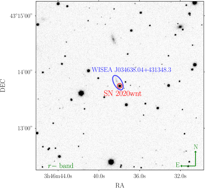
Figure 1: NOT $r-$band image of SN 2020wnt and its host galaxy, WISEA J034638.04+431348.3 The red circle marks the SN ($\textrm{RA}=03^{\rm h}46^{\rm m}37.\!\!^{\rm{s}}95$ $\textrm{Dec}=+43^{\circ}13^{\prime}45.\!\!^{\prime\prime}30$ (J2000)), while the blue ellipse marks its host galaxy. The orientation of the image is indicated in the bottom-right corner.

The host galaxy of SN 2020wnt is WISEA J034638.04+431348.3, a faint galaxy with no published redshift or distance information. The redshift adopted in our analysis is derived from the narrow emission lines (H$\alpha$, [O iii] $\lambda 5007$) visible in the SN spectrum. These lines give us a mean redshift of 0.032. Given the lack of independent measurements of distance to this galaxy, we estimate the uncertainty in our measurements assuming a peculiar velocity of $\pm 200$ km s^-1 (Tully et al., 2013). With these values, we compute a distance of $d=140.4\pm 3.0$ Mpc, which corresponds to a distance modulus of $\mu=35.74\pm 0.05$ mag. Figure 1 shows the NOT $r-$band image of SN 2020wnt and its host galaxy.

The Galactic reddening is quite high with $E(B-V)=0.42$ mag (Schlafly & Finkbeiner, 2011), while the host galaxy component is negligible. This is determined by the absence of narrow interstellar Na i D lines ($\lambda\lambda 5889$, 5895) at the rest wavelength of the host. As shown in section 3.4, the spectra of SN 2020wnt display a strong Na i D line, but it corresponds to the Milky Way component. Therefore, we assume that the reddening in the direction of SN 2020wnt is totally dominated by the Milky Way.

To characterise the global properties of the SN 2020wnt host galaxy, we got $griz$ photometry from the Pan-STARRS1 (PS1) public science archive. To obtain estimates of the stellar mass ($M_{*}$) and star formation rate (SFR), we use a custom galaxy spectral energy distribution (SED) fitting code, following the procedure detailed in Sullivan et al. (2010). The code is similar to z-peg (Le Borgne & Rocca-Volmerange, 2002), but uses the stellar population templates of pégase.2 (Fioc & Rocca-Volmerange, 1997). The best-fitting templates correspond to $M_{*}=\log\left(M/M_{\odot}\right)=8.22_{-0.12}^{+0.20}$ and $\log\left(\mathrm{SFR}\right)=-4.89_{-5.11}^{+3.09}$ M_⊙yr^-1. The large uncertainties obtained for the SFR are mainly associated to the lack of photometry in bluer bands (Childress et al., 2013). Such low stellar mass and star formation obtained for the host galaxy of SN 2020wnt are consistent with the expected range measured for other SLSN hosts (Neill et al., 2011; Chen et al., 2013; Lunnan et al., 2014; Leloudas et al., 2015; Perley et al., 2016; Schulze et al., 2018). In absence of a host spectrum, we could infer the metallicity through the mass – metallicity relation (e.g Tremonti et al., 2004). Following the prescriptions of Kewley & Ellison (2008), we derive a value that corresponds to 12 + log(O/H)$=8.17\pm 0.11$ dex in the O3N2 calibration and and 12 + log(O/H)$=8.18\pm 0.09$ dex in N2 calibration, respectively. These values suggest a low metallicity and are consistent with previous findings for SLSNe (e.g., Chen et al., 2017).

3.2 Light curves

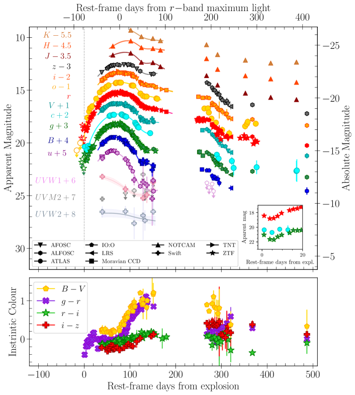
Figure 2: Top: UV, optical and NIR light curves of SN 2020wnt. Upper limits are presented as open symbols. The explosion time is indicated as a vertical dashed line. The photometry is corrected for Milky Way extinction using the Cardelli et al. (1989) extinction law. The solid lines show the Gaussian process (GP) interpolation before 180 days, and the shaded regions represent the errors from the GP. UV and $BVJHK$ photometry are in the Vega system, while $ugcroiz$ photometry is in the AB system. The inset plot shows the light curves in $gcr$ at very early phases. Bottom: Intrinsic colour curves of SN 2020wnt.

Figure 2 (top panel) shows the rest-frame multiband light curves of SN 2020wnt. The excellent photometric coverage during the first $\sim 320$ days from explosion allows us to constrain exceptionally well the light curve shape, magnitudes at maximum, rise times, and decline rates in the different bands. To estimate the main parameters of the light curves, we use Gaussian processes (GPs). For this procedure, we use the python package george (Ambikasaran et al., 2016), following the prescriptions of Gutiérrez et al. (2020a).

As seen in the top panel of Figure 2, SN 2020wnt evolves quite slowly and shows several distinctive properties during its evolution. The dense sampling in three of the four filters with very early observations ($gcr$) allows us to detect an initial peak, which is brighter in the bluer filters with an absolute magnitude of M${}_{g}=-17.71$ mag, M${}_{c}=-17.38$ mag, M${}_{r}=-17.30$ mag.

Following this initial peak, the $gcr$ light curves show a decrease in brightness (between 0.5 in $r$ and 0.7 mag in $g$). At this point, the SN reaches a minimum value, with absolute magnitudes of M${}_{g}=-17.00$ mag, M${}_{c}=-17.02$ mag, and M${}_{r}=-16.8$ mag at $\sim 4.9$ days. After this phase, a rise of $\sim 3.3-3.7$ mag is observed in all bands. A high cadence follow-up in the $uBgVriz$ bands starts after about 38 days from the explosion. This permits to cover the SN maximum in all optical bands.

Table 1: Light curve parameters of SN 2020wnt.

	Peak Abs. Mag	Rise time	$\Delta$M(${}_{\text{Peak}-130})$	$\Delta$M(${}_{77.5-130})$
Band	(mag)⋆	(days)⋆	(mag)†	(mag)
(1)	(2)	(3)	(4)	(5)
$u$	$-20.00\pm 0.02$	$61.3\pm 1.4$	3.58	3.25
$B$	$-20.27\pm 0.01$	$65.0\pm 2.2$	2.49	2.45
$g$	$-20.52\pm 0.03$	$72.0\pm 2.5$	2.27	2.25
$c$	$-20.50\pm 0.03$	$70.2\pm 1.4$	1.67	1.62
$V$	$-20.50\pm 0.02$	$72.4\pm 3.1$	1.69	1.65
$r$	$-20.52\pm 0.03$	$77.5\pm 3.1$	1.32	1.32
$o$	$-20.49\pm 0.01$	$75.0\pm 1.8$	1.29	1.29
$i$	$-20.40\pm 0.02$	$76.8\pm 5.1$	1.09	1.08
$z$	$-20.16\pm 0.01$	$79.0\pm 4.1$	0.81	0.81
$J$	$-20.84\pm 0.10$	$89.0\pm 5.2$	1.01	0.94
$H$	$-20.93\pm 0.08$	$93.8\pm 5.1$	0.72	0.55
$K$	$-20.92\pm 0.03$	$101.7\pm 1.0^{\ddagger}$	0.71	–

• Columns: (1) Band; (2) Peak absolute magnitudes; (3) Rise time; (4) Change in magnitude from the peak to 130 d from explosion; (5) Change in magnitude from 77.5 to 130 d from explosion.

• ^⋆ Peak absolute magnitudes and rise times were obtained from Gaussian Process (GP) fits. Magnitudes are corrected by the Milky Way extinction.

• ^† Change in magnitude from the peak. Note that each band reaches the peak at different times.

• ^‡ Due to the lack of data in $K$, the first point is assumed as the maximum and the uncertainty of the maximum time is the error from explosion epoch.

From the GP fits, we find that SN 2020wnt reaches the main peak in the optical bands between $\sim 61$ and 79 days from explosion (all phases stated in this paper are in the rest frame). The rise times are different in each band, with a faster rise in $u$ and a more extended rise in the NIR bands. The absolute magnitude peaks are around $-20.00$ mag in $u$ and $-20.93$ mag in $H$. In $gcVro$ the absolute peak magnitudes are around $-20.50$ mag. These values place SN 2020wnt at the bottom of the luminosity distribution of SLSNe-I (e.g. Angus et al., 2019). Table 1 shows the absolute peak magnitudes and the rest-frame rise times obtained in all optical and NIR bands.

One interesting characteristic observed in the light curves of SN 2020wnt is the behaviour around peak. In the redder bands, the SN reaches the maximum a bit later than in the blue bands, and the luminosity stays quasi-constant for a longer time, displaying a kind of "plateau". After maximum, the decline in the blue bands is much faster than in the redder ones. From the main peak to 130 days, the SN dims by $\sim 3.58$ mag in the $u$ band, $2.27$ mag in $g$ and $1.32$ mag in $r$ (almost three times slower than $u$). As the $u$ peak occurs before than the peak in $g$ and $r$ (61.3, 72.0, and 77.5 days in $u$, $g$ and $r$, respectively), we can better compare these decreases by fixing a range of time. Measuring the change in magnitude from 77.5 days (the epoch of $r-$band peak) to 130 days, we see that the SN dims by $\sim 3.26$ mag in $u$ and $2.25$ mag in $g$. The decline rates in these two ranges are also presented in Table 1. Moreover, in the $UVW1$ and $UVW2$ bands, we see a flattening or upturn, which may be attributable to the known red leak. Meanwhile, for the $UVM2$ filter, which is not affected by the red leak, we only measure upper limits. Therefore, the evolution of the Swift UV bands indicates a decline in the UV flux and the emergence of an optically dominated spectral energy distribution (SED) ${\sim}100$ days post explosion.

After $\sim 130$ days, the drop in brightness slows down. Fitting a line to the observations obtained between 130 and 180 days (the last observation before the SN went behind the sun), we measure a slope of $1.01\pm 0.03$ mag per 100 days in $r$, and $1.18\pm 0.01$ per 100 days in $i$. The monitoring of SN 2020wnt restarted at 247 days in $r$, and a couple of days later in $BgVcizJHK$. With the new data, we again fit a line to the data between 130 and 275 days and we found slower declines, with slopes of $0.90\pm 0.01$ mag per 100 days in $r$ and $0.99\pm 0.06$ mag per 100 days in $i$. These values are very close to those expected from the ⁵⁶Co decay (0.98 mag per 100 days; Woosley et al. 1989). Starting from 273 days, the SN is found to experience a drastic and sudden drop in brightness in all bands. Within $\sim 35$ days, the magnitudes decrease by about $1.5$ mag. Fitting a line after 273 days in the $r-$band, we find a slope of $4.5\pm 0.3$ mag per 100 days. From $\sim 320$ days, fluctuations in brightness are observed both in the optical and the NIR bands.

The intrinsic colour curves of SN 2020wnt are presented in the bottom panel of Figure 2. During the first $\sim 35$ - 40 days, we can only infer $g-r$ colour information. In $\sim 20$ days, SN 2020wnt becomes redder, going from a $g-r=-0.41$ mag to $g-r=0.16$ mag. The $g-r$ colour shows an initial peak at 21.3 days. After this, the SN goes back to bluer colours, reaching a value of $g-r=-0.09$ mag at 42.5 days. From this epoch, the $g-r$ colour shows a quasi flat evolution up to $\sim 70$ days. Later than 70 days, the SN becomes redder again, reaching its main peak at 135.4 days with a colour of $g-r=1.10$ mag. A gap in the observations prevented us from monitoring the SN evolution between 151 and 251 days, however, when the SN is recovered, we measure a colour of $g-r=0.10$ mag showing that SN 2020wnt became bluer again, but after this, it gets redder one more time.

Starting from $\sim 38$ days, we also have the $B-V$, $r-i$ and $i-z$ colours. $B-V$ shows a similar behaviour than that observed in $g-r$, but with redder colours at all phases. Unlike $g-r$ and $B-V$, the evolution of $r-i$ and $i-z$ shows little variation. Overall, they tend to be bluer up to $\sim 150$ days. Of these two, the colour change is more significant in $i-z$, going from $-0.22$ to $0.12$ mag (at $\sim 150$ days) in comparison to the evolution from $-0.13$ to $0.16$ mag in $r-i$. After the gap, the SN gets bluer in $B-V$, $r-i$ and $i-z$. This tendency is clear until 320 days. From there, the temporal coverage does not allow us to estimate a trend.

3.3 Bolometric light curve

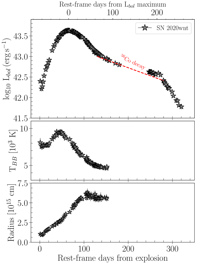
Figure 3: Top: Bolometric light curve of SN 2020wnt. The dashed red line shows the luminosity expected from ⁵⁶Co decay (assuming full trapping). Middle: Temperature evolution of SN 2020wnt. Bottom: Evolution of blackbody radius of SN 2020wnt. Error bars are comparable to the size of the symbols.

To build the bolometric light curve of SN 2020wnt using our reddening corrected photometry from UV to NIR bands, we employ the superbol code (Nicholl, 2018). In order to have a similar coverage in the different bands at the same epochs, we interpolate and extrapolate the light curves assuming constant colours and using the $r-$band as a reference filter from explosion to 320 days after the explosion. We converted all magnitudes to flux and construct the SED at all epochs. We computed multiple pseudo-bolometric light curves by performing trapezoidal integration just in the optical and NIR bands, and UV + optical + NIR. We also calculated a full bolometric light curve by fitting a blackbody to the SED. When comparing the bolometric light curve from UV to NIR with that obtained by extrapolating the SED constructed from the optical and NIR bands, we find that they are consistent. The bolometric light curve is presented in the top panel of Figure 3.

Following the process described in Section 3.2, we use a GP to estimate the main parameters in the bolometric light curve. We find a peak luminosity of $L_{bol}=4.25(\pm 0.30)\times 10^{43}$ erg s^-1 at 65 days. This maximum occurs earlier than most of the peaks obtained from the optical and NIR bands, except for the $uB$ filters. Between 140 and 270 days, the light curve declines at a rate of $0.77\pm 0.02$ mag per 100 days. After that, we estimate a decline rate of $4.07\pm 0.01$ mag per 100 days.

From superbol, the blackbody temperature (T_BB) and radius (R_BB) are also obtained by fitting the SED of each epoch with a blackbody function. Figure 3 (middle and bottom panels) shows the temperature and radius evolution from explosion to $\sim 150$ days. At early times the temperature is relatively low, with a value of T${}_{BB}\approx 8000$ K. The temperature increases and reaches a value of T${}_{BB}\approx 10000$ K at $\sim 51$ days from explosion, and then it decreases. On the other hand, the radius shows a continuous increase up to 105 days, where it reaches its maximum value (R${}_{BB}=6.2\times 10^{15}$ cm). Fitting a line between explosion and the maximum value, we find a slope of $\sim 6000$ km s^-1. After this peak, the radius shows a slow and steady decline to $5.5\times 10^{15}$ cm.

3.4 Spectral evolution

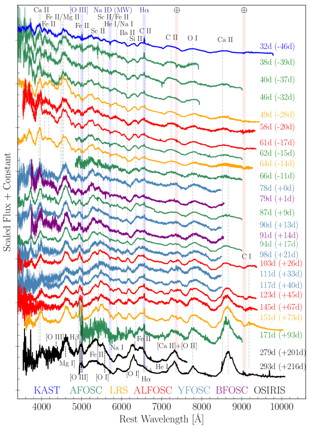
Figure 4: Spectral sequence of SN 2020wnt from 32 to 293 days from explosion in the rest-frame. The phases are labelled on the right. The numbers in parentheses are the phases with respect to the maximum light in the $r-$band. Each spectrum has been corrected for Milky Way (MW) reddening and shifted vertically by an arbitrary amount for presentation. The colour of the spectra represents the different instruments used to obtain the data. The vertical dashed lines indicate the rest position of the strongest lines, vertical blue lines indicate emission lines from the host galaxy ([O iii] and H$\alpha$) and the narrow Na i D interstellar feature from the MW, and the pink lines indicates the position of the telluric absorption ($\oplus$ symbol). In the last two spectra, narrow emission lines from the host galaxy (H$\alpha$, H$\beta$, [O iii], [N ii], and [S ii], visible in grey) were removed for presentation.

Figure 4 shows the spectral evolution of SN 2020wnt  covering the phases from 32 to 293 days after explosion. The slow evolution detected in the light curves is also visible in the spectra, where a blue continuum is observed for around 100 days. The first spectrum taken at 32 days ($-46$ d from the maximum light in the $r$ band) and used for the classification, is dominated by strong lines of O i $\lambda 7774$, Ca ii (H&K and NIR triplet), Si ii $\lambda 6355$, and C ii $\lambda 6580$, $\lambda 7235$. Na i D /He i and the Fe ii $\lambda 4924$, 5018, 5169 lines are also clearly detected. From 32 to 78 days after explosion, there are limited changes in the spectra, with small variations in the relative line intensities. More precisely, C i $\lambda 6580$ and $\lambda 7235$ and Na i D /He i become weaker, while the Fe ii $\lambda 4924$, 5018, 5169 lines become stronger. During this period, the spectra do not show signs of O ii lines. After 78 days, the Na i D /He i line vanishes while the flux in the bluer part of the spectra shows a significant decrease, mainly due to the line blanketing. After this epoch, a ’W’-shape profile is visible around 4800 Å. This feature has been previously detected in several SNe Ic (e.g. SN 2004aw; Taubenberger et al. 2006; SN 2007gr; Valenti et al. 2008b; Hunter et al. 2009; Chen et al. 2014) and SLSNe (e.g. SN 2015bn; Nicholl et al. 2016a).

To support our preliminary line identification in SN 2020wnt, we employ the synow code (Fisher, 2000) and the best quality spectra at 49 days ($-28$ days from the $r-$band maximum) and 87 days ($+9$ days from the $r-$band maximum). For the spectrum before peak, we assume a blackbody temperature of $T_{\text{bb}}=10800$ K and a photospheric velocity of $v_{\text{ph}}=8000$ km s^-1, while for the spectrum after peak, we use a $T_{\text{bb}}=8000$ K and a photospheric velocity of $v_{\text{ph}}=6000$ km s^-1. To reproduce the observed features in both spectra, we include the lines of Ca ii, O i, Si ii, C ii, Na i, Fe ii, Sc ii, Ba ii, Mg ii and Ti ii. As shown in Figure 5, the synthetic spectra at 49 and 87 days reproduce relatively well the observed features of SN 2020wnt, allowing us to confirm the presence of C ii and Si ii.

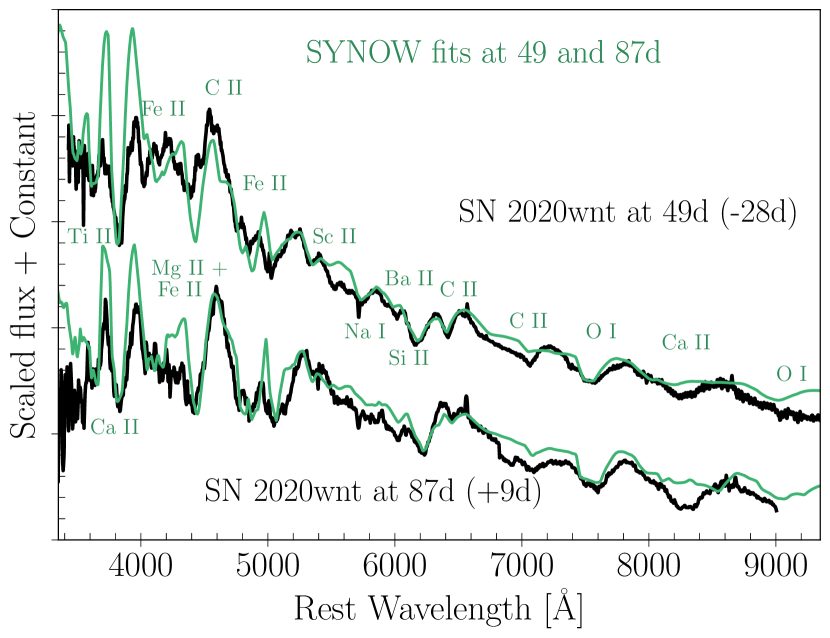
Figure 5: Spectral comparison of SN 2020wnt at 49 and 87 days from explosion ($-28$ and $+9$ from maximum, respectively) and the synow fits. The synow synthetic spectra (green) are overplotted on the observed spectra (black).

Returning to the spectroscopic evolution, we see that from day 87 (+9 days from maximum), the Ca ii NIR triplet and O i become stronger, and the region below 5500 Å is almost entirely dominated by the iron-group lines. At 103 days, the C ii $\lambda 6580$ and $\lambda 7235$ lines disappear while the continuum becomes redder. We detect a feature at $\sim 9000$ Å that is possibly due to C i $\lambda 9183$. As the temperature decreases, C i lines start to be detected.

After 123 days (+45 from the peak), SN 2020wnt starts the transition to the nebular phase. This is indicated by the Ca ii NIR triplet, which shows signs of an emission component. From 123 to 171 days, the spectral evolution is slow. The most significant difference is the strengthening of the emission component in the Ca ii NIR triplet, as well as in the lines detected at $\sim 4600$ Å, $\sim 6000$ Å, and $\sim 7300$ Å.

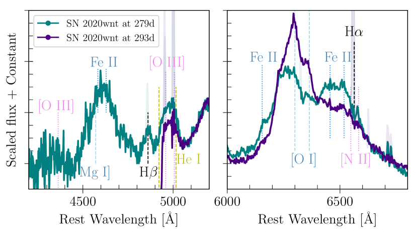
Figure 6: Observed emission profiles of SN 2020wnt at 279 and 293 days from explosion. Vertical lines indicate the rest position of the strongest lines. Left panel: Emission profiles between 4200 and 5200 Å. Right panel: Emission profiles between 6000 and 6800 Å.

The last two spectra of SN 2020wnt were obtained at 279 and 293 days ($+201$ and $+216$ days from the peak), once the SN returned from behind the Sun. At 279 days, the spectrum shows emission lines of [Ca ii] $\lambda\lambda 7291$, 7324 with the possible contribution of [O ii] $\lambda\lambda 7320$, 7330), [O i] $\lambda\lambda 6300$, 6364, [O i] $\lambda 5577$, Na i, Mg i] $\lambda 4571$ plus Fe ii, a weak feature near $\sim 7100$ Å, possibly caused by He i $\lambda 7065$, and a broad emission at $\sim 5000$, which could be identified as either the broad [O iii] $\lambda 4959$, $\lambda 5007$ components, Fe ii, He i or [Fe ii]. We explored all these identification scenarios and concluded that this feature is probably caused by [O iii] $\lambda 4959$, $\lambda 5007$ with some contribution of He i (see Figure 6). Despite the bluer part of the spectrum is a bit noisy, we clearly see an emission line produced by Ca ii H&K. An excess around 4300 Å is noticed and could be consistent with [O iii] $\lambda 4363$.

One remarkable characteristic in this phase is the identification of an emission line on the red side of [O i] $\lambda\lambda 6300$, 6364, which could be caused either by H$\alpha$, Fe ii $\lambda 6456$, 6518 or [N ii] $\lambda\lambda 6548$, 6583. Fitting a Gaussian, we find that the line is centred at $\sim 6480$ Å. If this feature is caused entirely by either H$\alpha$ or [N ii], a significant blueshift ($>3000$ km s^-1) has to be taken into account, while for Fe ii, the wavelength match is satisfactory. The possible detection of Fe ii $\lambda 6155$ could support this hypothesis. However, a broad line at the position of H$\beta$ is also found, which suggests that H$\alpha$ should contribute to the boxy feature. Therefore, this boxy emission line is probably a result of blended lines of Fe ii, H$\alpha$, and probably [N ii]. A zoom around the H$\alpha$ and H$\beta$ regions is presented in Figure 6.

The last spectrum, at 293 days, displays the same lines as the spectrum at 279 days (from 5000 Å) plus emission features of the Ca ii NIR triplet and O i $\lambda 7774$ (detected thanks to the larger wavelength coverage). With the identification of these features, we deduce that the strongest line at this phase is the Ca ii NIR triplet. From 279 to 293 days, the spectra display two major changes, related to the decrease in the intensity of the lines near 5300, 6155 Å (Fe ii) and 6500 Å (the boxy emission line). The consistent decrease in the strength of these lines supports the idea that the Fe ii $\lambda 6456$, 6518 lines should contribute to the line emission observed on the red side of [O i] $\lambda\lambda 6300$, 6364.

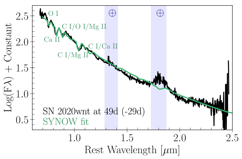
Figure 7: NIR spectrum of SN 2020wnt (black) obtained at $\sim 49$ days from explosion ($-29$ days from peak) with SpeX compared with the synow fit. Regions of strong telluric absorption are masked in blue.

Figure 7 shows a NIR spectrum obtained at $\sim 49$ days from explosion ($-29$ days from peak), covering a wavelength range between 0.63 and 2.5 $\mu$m. At this phase, the spectrum displays a blue continuum with clear features of O i, Ca ii, previously identified in the optical spectra, plus multiple features of C i. We also detect an absorption line at $\sim 1.05$ $\mu$m that could be either He i 1.083 $\mu$m, C i 1.069 $\mu$m, or even a mix of them. If this line is due to He i, we would also see a clear line detection near 2.058 $\mu$m; however, this is not the case. The lack of this line suggests that the contribution of He i to the 1.05 $\mu$m absorption is small. Similarly, the absorption features at 1.26 and 2.12 $\mu$m could be also produced by C i. There are several carbon lines near those wavelengths (see Millard et al. 1999; Valenti et al. 2008b; Hunter et al. 2009).

To identify the ions that produce the lines in the NIR, we create a synthetic spectrum with synow by using the same parameters as mentioned before. We consider a blackbody temperature of $T_{\text{bb}}=10800$ K and a photospheric velocity of $v_{\text{ph}}=8000$ km s^-1. We reproduce the observed spectrum only including Ca ii, O i, C i and Mg ii, as shown in Figure 7, but beyond 1.8 $\mu$m none of the ions seems to produce absorption lines. The identification of C lines in the NIR reinforces the idea that SN 2020wnt has a carbon-rich progenitor.

3.5 Expansion velocities

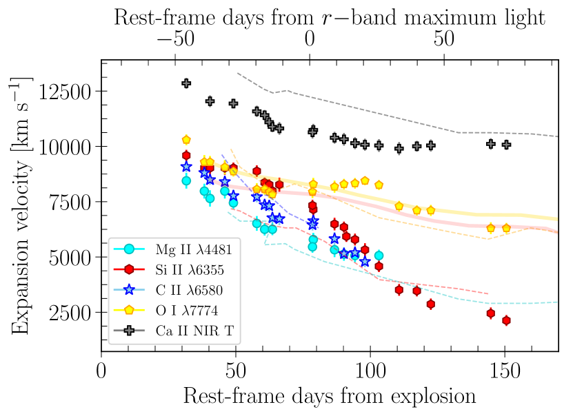
Figure 8: Evolution of expansion velocities derived from the minimum flux of several absorption lines of SN 2020wnt (see Gutiérrez et al., 2017, for details in the estimation of velocities and their uncertainties). For comparison, we also include the Si ii and O i velocities of the SLSN 2015bn (solid lines), and the velocities of the carbon-rich type Ic SN 2007gr (dashed lines). For this object, we stretched the time by a factor of 4 ($t=4\times t_{0}$). This factor is obtained from the light curve analysis (see Section 4.3).

We measure the expansion velocities of the ejecta for five spectral lines (Mg ii, Si ii, C ii, O i and Ca ii NIR triplet) using the spectra covering the phases from 32 and 151 days from explosion. These velocities were obtained from the minimum flux of the absorption component and are presented in Figure 8. In this analysis, we do not include the iron lines (Fe ii $\lambda 4924$, 5018, 5169 Å) due to complications in estimating their velocities as these lines seem to be blended with other ions. Figure 8 shows that the evolution of the expansion velocities can be split into two groups: one characterised by an initial decrease that then flattens, and a second group that shows a monotonic decline with time. In the first group, we find Ca ii NIR triplet and O i, whereas Mg ii, Si ii and C ii are found in the second group. In addition to this behaviour, we also see that the first group shows higher velocities, suggesting that the Ca ii NIR triplet and O i lines mostly form in the outer part of the ejecta, while the Mg ii, Si ii and C ii lines form in the inner layers. The Ca ii NIR triplet has the highest expansion velocities, decreasing from $\sim 12800$ km s^-1 at 32 days to $\sim 10100$ km s^-1 at 151 days. On the other hand, Si ii decreases from 9600 km s^-1 to just 2100 km s^-1.

For comparison, in Figure 8 we include the expansion velocities of the carbon-rich type Ic SN 2007gr (Hunter et al., 2009) corrected by a temporal factor of $\sim 4$ in order to match the overall evolution of SN 2020wnt (See Section 4.3), and the Si ii and O i velocities of the SLSN 2015bn (Nicholl et al., 2016a). Overall, the velocities of SN 2020wnt and SN 2007gr are comparable, except for that inferred from the Ca ii NIR triplet, which has higher values in SN 2007gr. When comparing SN 2020wnt with SN 2015bn, we see that the O i velocities are very similar, but the Si ii velocities show a completely different behaviour. While the velocities of SN 2015bn shows a slow drop, in SN 2020wnt we notice a more rapid decrease. The velocity values for all objects are low compared to those observed in typical SNe Ibc (e.g. Prentice et al., 2019) and SLSNe, respectively. Similarly, low velocities were also found for SN 2007gr (Hunter et al., 2009) and SN 2015bn (Nicholl et al., 2016a).

4 Comparison with other SNe

SN 2020wnt is a hybrid object sharing the properties of both SLSN and SN Ic classes. The light-curve morphology is comparable to that observed in several SLSNe (pre-peak bumps, long rise to the main peak, slow evolution); with absolute magnitude at peak within the luminosity distribution of SLSNe-I, although at the lower end (De Cia et al., 2018; Angus et al., 2019). Despite this, SN 2020wnt is brighter ($\sim-20.5$ mag) compared to standard SNe Ic (peak absolute magnitudes ranging between $-17$ and $-18$ mag; e.g. Taddia et al. 2018b), but lies in the luminosity range studied by Gomez et al. (2022) for luminous SNe. On the other hand, the spectra are more similar to the type Ic class than to SLSNe. This similarity is founded on the absence of the O ii lines (one of the features characterising SLSNe), and the strength of different lines, such as the Ca ii NIR triplet, Si ii and C ii lines. A major difference between SN 2020wnt and SNe Ic is the slow evolution observed in the spectra, which is consistent with SLSNe-I. Given these hybrid properties, we compare SN 2020wnt with both SLSNe and SNe Ic. These are well observed slow-evolving SLSNe, SLSNe with pre-peak bumps, SLSNe with C ii lines in their spectra, and two very well sampled type Ic SNe. Details of the comparison sample are presented in Table 2.

Table 2: Detailed properties of the comparison sample.

SN	Redshift	E(B$-$V)MW	Characteristics⋆	References†
		(mag)
SLSNe
SN 2006oz	0.376	0.042	Bumpy	(1)
SN 2007bi	0.127	0.028	Slow	(2), (3)
PTF12dam	0.107	0.012	Slow; C ii	(4), (5), (6)
LSQ14an	0.1637	0.074	Slow	(7)
LSQ14bdq	0.345	0.056	Bumpy	(8)
DES14X3taz	0.608	0.022	Bumpy	(9)
SN 2015bn	0.1	0.022	Slow	(10), (11)
DES15S2nr	0.22	0.030	Bumpy	(12)
SN 2017gci	0.0873	0.116	Slow; C ii	(13)
DES17X1amf	0.92	0.022	Bumpy	(12)
SN 2018bsz	0.0267	0.214	Bumpy; C ii	(14), (15), (16)
SNe Ic
SN 2004aw	0.0163	0.022	–	(17)
SN 2007gr	0.0017	0.055	C ii	(18), (19), (20)

• ^⋆Characteristics: Slow: Slow-evolving SLSNe; Bumpy: SLSNe with pre-peak bumps; C ii: C ii lines in the spectra.
  

• ^†References: (1) Leloudas et al. (2012); (2) Gal-Yam et al. (2009); (3) Young et al. (2010); (4) Nicholl et al. (2013); (5) Chen et al. (2015); (6) Vreeswijk et al. (2017); (7) Inserra et al. (2017); (8) (Nicholl et al., 2015b); (9) Smith et al. (2016); (10) Nicholl et al. (2016a); (11) Nicholl et al. (2016b); (12) Angus et al. (2019); (13) Fiore et al. (2021); (14) Anderson et al. (2018); (15) Chen et al. (2021); (16) Pursiainen et al. (2022); (17) Taubenberger et al. (2006); (18) Valenti et al. (2008b); (19) Hunter et al. (2009); (20) Chen et al. (2014).

4.1 Light curve comparison

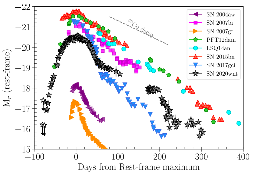
Figure 9: Comparison of the $r-$band light curves of SN 2020wnt with the slow-evolving SLSNe SN 2007bi, PTF12dam, LSQ14an SN 2015bn, and SN 2017gci, and the type Ic SN 2004aw and SN 2007gr (given as reference). All SLSNe have been K-corrected to rest-frame. Only corrections for Milky Way extinction have been applied.

Figure 9 shows the $r-$band absolute light curve of SN 2020wnt compared to five well-sampled slow-evolving SLSNe-I and two normal SNe Ic. From the comparison, the evolution of SN 2020wnt is similar to that observed in SN 2017gci (this object has characteristics of both slow- and fast-evolving SLSNe-I; Fiore et al. 2021). Excluding the type Ic SNe 2004aw and 2007gr, which are evidently faint, SN 2020wnt is the faintest object in the (SLSN-I) sample. It is $>1$ mag fainter than the brightest object, SN 2015bn. Inspecting the evolution at the early phases, we notice incomplete information for the SLSN-I sample. Therefore, it is hard to know the rise-time duration and how these objects evolve at very early phases, i.e., if they show an initial peak (bump) or not. The only objects with an early detection were PTF12dam and SN 2015bn. For SN 2015bn, Nicholl et al. (2016a) estimated a rise time of 79 days, while for SN 2020wnt, we estimate a rise time of $\sim 77.5$ days in $r$. These rise times are among the longest presented to date.

Analysing the shape of the light curve, we see that SN 2020wnt and SN 2017gci have a similar behaviour. After maximum, the decline slope of both objects changes at $50-55$ days from peak. Later, a shoulder is observed. For SN 2020wnt, after $\sim+50$ days from peak, the decline rate is comparable to that expected from the ⁵⁶Co decay (see Section 3.2). This evolution is observed until $\sim+200$ days from peak. After this, the slope changes again, showing a very fast linear decline.

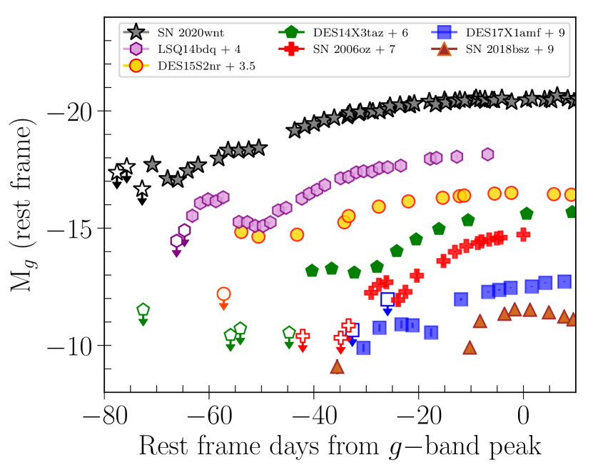
Figure 10: Rest-frame, $g-$band light curve of SN 2020wnt compared with SLSNe showing pre-peak bumps: SN 2006oz, LSQ14bdq, DES14X3taz, DES15S2nr, DES17X1amf, and SN 2018bsz.

As mentioned in Section 3.2, the $gcr-$band light curves of SN 2020wnt have an initial bump with a relatively short duration. To analyse the pre-peak bump in SN 2020wnt, we compare the $g-$band early light curve with a sample of SLSNe that show signs of an early bump. This comparison is presented in Figure 10. To easily examine these objects, we arranged the light curves in terms of the rise-time to the main peak. SN 2020wnt has the longest rise time ($\sim 72$ days), while SN 2018bsz has the shortest one (around 10 days). An opposite behaviour is observed in the duration of the initial peak. Here, SN 2020wnt shows the shortest bump with a duration $<5$ days, while the longest initial bump is observed for SN 2018bsz ($>25$ days; see Anderson et al. 2018 for better constraints in other bands). In terms of luminosity, we find that LSQ14bdq is the most luminous object, DES15S2nr is the least luminous, followed by SN 2020wnt and SN 2018bsz, which have similar absolute magnitudes at peak.

4.2 Spectral comparison

Figure 11: SN 2020wnt at around maximum light (top) and at $\sim+50$ days from $r-$band maximum (bottom) compared with well-sampled slow-evolving SLSNe: SN 2007bi, PTF12dam, LSQ14an, SN 2015bn, and SN 2017gci. Each spectrum has been corrected for Milky Way reddening and shifted vertically by an arbitrary amount for presentation. Vertical lines indicate the rest position of the strongest lines. The phases and SN names are labeled on the right.

The spectral comparison of SN 2020wnt and slow-evolving SLSNe-I is presented in Figure 11. To examine the similarities and differences between these objects, we select two reference epochs: around peak (top) and $\sim+50$ from maximum light (bottom). Firstly, we notice a large diversity. Around peak, SN 2020wnt has a distinct spectrum, dominated by strong absorption lines. In particular, the W-shape profile due to Fe lines is a remarkable characteristic. Though the spectral coverage does not allow to see the full profile of the Ca ii NIR triplet, based on the spectra before and after peak (Figure 4), this line is intense in SN 2020wnt, but it seems to be absent in the other objects. Only a few common features are identified among SN 2020wnt and the comparison sample: C ii lines with SN 2017gci, and Si ii and O i lines with SN 2015bn.

At around $+50$ days from maximum light, the spectra are still quite heterogeneous, although SN 2020wnt and SN 2017gci look more alike than before. This is seen in the bluer part, with the blended feature due to the Mg ii and Fe ii lines, and in the redder part, with the detection of strong features of O i and Ca ii NIR triplet. Both SN 2020wnt and SN 2015bn still share similar profiles of Si ii and O i. Fe ii and O i are visible in all objects. In contrast to the photometric behaviour, the spectrum of SN 2020wnt seems to evolve slower than that of SN 2007bi and LSQ14an. At the later phase, these objects show clear signs of nebular lines (e.g. [Ca ii] + [O ii]), while SN 2020wnt still shows lines of the photospheric phase.

4.3 Comparison with SN 2015bn and SN 2007gr

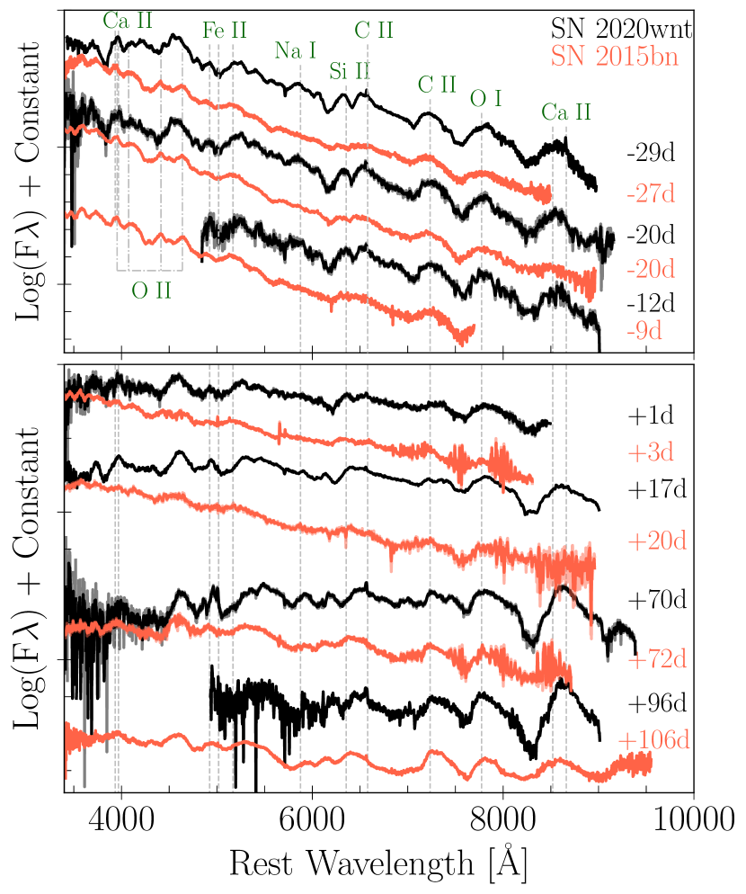
Figure 12: Spectral comparison of SN 2020wnt with the slow-evolving SN 2015bn at eight different epochs before (top panel) and after (bottom panel) the maximum light in the $r-$band. Each spectrum has been corrected for Milky Way reddening and shifted vertically by an arbitrary amount for presentation. Vertical lines indicate the rest position of the strongest lines. The phases are labeled on the right.

We now compare SN 2020wnt with the most extreme objects shown in Figure 9: SN 2015bn, the brightest object in the comparison sample and one of the best observed SLSNe to date, and the carbon-rich type Ic SN 2007gr, the faintest SN in the plot, and the best-spectral match object found by gelato (Harutyunyan et al., 2008).

The spectral comparison between SN 2020wnt and SN 2015bn at seven different epochs is presented in Figure 12. Before the peak (top panel), the spectra of both objects are characterised by a blue continuum with lines of O i, Si ii, C ii and Fe ii. In SN 2020wnt, these features are stronger at all phases. In contrast, the main differences lie in the O ii and Ca ii lines. The spectra of SN 2020wnt do not show the W-shape O ii features as observed in SN 2015bn, and other SLSN-I events. The presence/absence of these lines depends on the temperature (more details in Section 6). Unlike SN 2015bn, SN 2020wnt shows very strong Ca ii absorptions. These Ca ii absorption features are not observed in young SLSNe-I. After peak (bottom panel), in contrast with SN 2015bn, SN 2020wnt has a redder continuum, more intense lines and the bluer part of the spectrum is dominated by Fe-group lines. Some signs of emission components are also detected, suggesting the beginning of the transition to the nebular phase. All these properties are delayed in SN 2015bn.

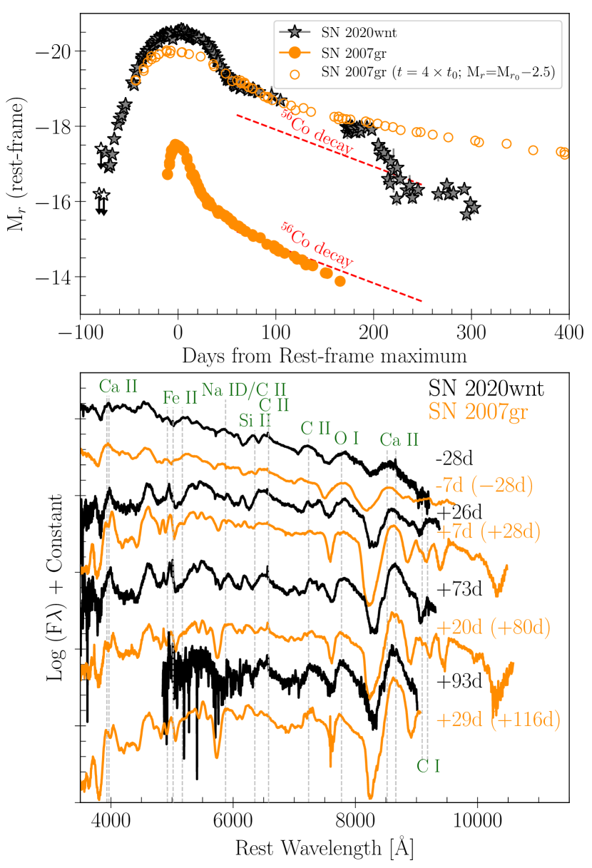
Figure 13: Light curve and spectral comparison with the type Ic carbon-rich SN 2007gr. Top: Comparison of the $r-$band light curves. For the light curve of SN 2007gr, we applied a temporal correction ($t=4\times t_{0}$) to reproduce the same shape and width as SN 2020wnt. A shift of 2.5 mag is applied to the magnitude in order to have a similar brightness in the transition and the tail (from $\sim+53$ days from peak). Bottom: Spectral comparison at four different epochs from the $r-$band maximum. Each spectrum has been corrected for Milky Way reddening and shifted vertically by an arbitrary amount for presentation. Vertical lines indicate the rest position of the strongest lines. The rest-frame phases are labeled on the right, while the epochs with the temporal correction (for SN 2007gr, $t=4\times t_{0}$) are in parenthesis. This correction gives a consistent epochs to SN 2020wnt.

In Figure 13, we compare SN 2020wnt and the type Ic carbon-rich SN 2007gr. Although the light curves (top panel) of these two objects are completely different at the first glance, they share a similar spectroscopic evolution (bottom panel) with some time lag ($t=4\times t_{0}$; where $t_{0}$ is the rest-frame maximum of SN 2007gr), which was initially found by the spectral matching from gelato. From the light curves in the $r-$band, we estimate that SN 2020wnt is $\sim 3$ mag brighter than SN 2007gr around the maximum light. SN 2020wnt also has a pre-peak bump light curve morphology and evolves on a much longer timescale than its fainter counterpart. In order to have a broad light curve similar to that of SN 2020wnt, we applied a temporal correction to SN 2007gr. We find that a factor of 4 can reproduce the light curve width of SN 2020wnt, and it is, in turn, in agreement with that found by the spectral matching. This correction is included in the top panel of Figure 13 (open orange circles).

In the bottom panels of Figure 13, the spectroscopic comparison between SN 2020wnt and SN 2007gr is presented at four different epochs. Analysing the spectral features, one sees that the main similarity is the detection of the carbon lines, while the main difference is the strength of the Na i line, which is more intense in SN 2007gr. From the spectral matching with gelato, we found a time lag of $t=4\times t_{0}$. Therefore, the SN 2020wnt spectrum at $-27$ days from peak is compatible with that of SN 2007gr at $-7$ days from peak. Both SNe show strong features of Ca ii, O i, and the clear signs of Si ii, C ii and the W-shape Fe ii lines at around 4800 – 5200 Å. After peak, both objects evolve maintaining the time lag identified in the spectra before peak, which is consistent with that obtained from the light curves. The similarity in the spectral evolution suggests that both objects may arise from a carbon-rich progenitors, however, the longer timescale and the brightness of the light curve may suggest different explosion parameters.

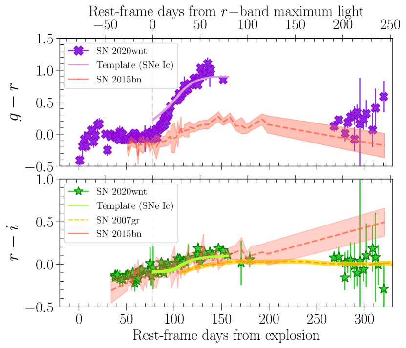
Figure 14: $g-r$ and $r-i$ colour curves of SN 2020wnt. For comparison, in solid lines (purple and green) we show the intrinsic SNe Ic colour-curves templates ($g-r$ and $r-i$) from Stritzinger et al. (2018) multiplied by a temporal factor of 4 ($t=4\times t_{0}$). We also include the $r-i$ colour of SN 2007gr (multiplied by the temporal factor; dashed orange line) and the $g-r$ and $r-i$ colours of SN 2015bn (dashed light red line; Nicholl et al. (2016a)). The data used here for SN 2007gr were taken from Bianco et al. (2014).

In Figure 14, we compare the $g-r$ and $r-i$ colours of SN 2020wnt, SN 2015bn and SN 2007gr (applying the temporal correction previously mentioned). In $g-r$, we find that from the maximum light, the evolution of SN 2020wnt and SN 2015bn are very different. While SN 2020wnt evolves quickly to the red, reaching a peak $\sim 50$ days later, SN 2015bn remains bluer a much longer time. At later phases, the colours are more alike. On the other hand, the $r-i$ colours are almost identical in the three objects up to $+150$ days from the maximum (SN 2007gr being the bluest). After this, the evolution diverges. For instance, SN 2020wnt and SN 2007gr become a bit bluer, whereas SN 2015bn evolves to the red. In Figure 14, we also include the intrinsic colour templates of SNe Ic from Stritzinger et al. (2018). To these templates, we apply the same temporal corrections as that found for SN 2007gr. From this comparison, 1) using these templates to constrain the host extinction, we find that for SN 2020wnt it is negligible; 2) the colour of SN 2020wnt between the maximum light and $+40$ days from the maximum (temporal correction included), evolves similarly as SNe Ic in both $g-r$ and $r-i$. This suggests that the colour of SN 2020wnt is similar to that observed in standard SNe Ic but on a longer timescale.

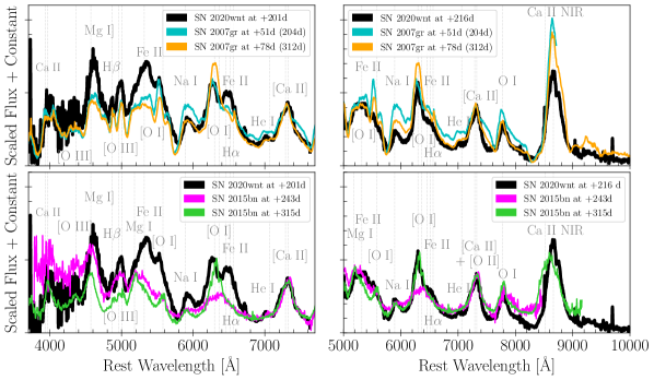
Figure 15: Spectral comparison between SN 2020wnt and SN 2007gr (top) and SN 2020wnt and SN 2015bn (bottom). Each spectrum has been corrected for Milky Way reddening. Spectra are scaled to match the [Ca ii] line. Vertical lines indicate the rest wavelengths of the strongest lines. The phases are labeled in the legend. In SN 2020wnt, the narrow emission lines from the host galaxy were removed for presentation. For SN 2007gr the phases in brackets correspond to the epochs with the temporal corrections ($t=4\times t_{0}$).

In Figure 15, we compare the late phase spectra of SN 2020wnt with those of SN 2007gr (top) and SN 2015bn (bottom) at similar epochs. As before, we find that the comparison with SN 2007gr has a time lag of $t=4\times t_{0}$, i.e., the spectrum of SN 2020wnt at $+201$ days from peak is similar to the spectra of SN 2007gr after 50 days from peak. In the top panel of this Figure, we compare our spectra at $+201$ days (blue part, left panel) and $+216$ days (red part, right panel) with SN 2007gr at $+51$, and $+78$ days from peak (with the correction the epochs are $+204$, and $+312$). Analysing the blue part (left panel), we see that both objects have the similar lines, but they seem to be stronger in SN 2020wnt. The shoulder on the red side of [O i] $\lambda\lambda 6300$, 6364 is also detected in SN 2007gr, though a bit fainter. From the red part (spectrum at $+216$ days, right panel), the lines observed in both objects fit very well. The larger discrepancy is in the intensity of the Ca ii NIR triplet feature, which is stronger at all epochs in SN 2007gr. At this phase, the shoulder of the red side of the [O i] line matches better than before.

In the bottom panel of Figure 15, we present the late spectra of SN 2020wnt and SN 2015bn. For SN 2015bn we use two epochs ($+243$ and $+315$ days from peak) that have some similarities with our spectra. Examining the blue part of the spectra, we notice some differences between these two objects. For instance, in the three spectra of SN 2015bn, there are no signs of a feature on the red side of [O i] $\lambda\lambda 6300$, 6364, of the emission around 5300 Å (attributed to Fe ii) and the line at $\sim 7100$ Å (possibly He i) detected in SN 2020wnt. Now, the red part (right panel) is similar, although SN 2020wnt has a stronger Ca ii NIR triplet, but a weaker O i than SN 2015bn at all epochs. Overall, the SN 2015bn spectrum that best matches SN 2020wnt is that at $+315$ days. The similarity of the nebular spectra of SN 2020wnt with those of SN 2007gr and SN 2015bn suggests that these objects are related, and they possibly have a common origin, including a similar chemical composition.

5 Explosion and progenitor scenarios

5.1 Nebular properties

To constrain the internal conditions and core structure of SN 2020wnt, we investigate the nebular spectra in detail. Based on the findings of Jerkstrand et al. (2014), the O i mass responsible for the line emission can be estimated from the oxygen luminosity, as follows:

M${}_{O}=\frac{L_{6300,6364}/\beta_{6300,6364}}{9.7\times 10^{41}~{}\mathrm{erg~{}s^{-1}}}\times exp(\frac{22720~{}K}{T})$ M_⊙

where L_6300,6364 is the line luminosity of [O i] $\lambda\lambda 6300$, 6364, $\beta_{6300,6364}$ is the is the Sobolev escape probability, and T is the temperature. Here, the temperature can be derived from the [O i] $\lambda 5577$ to [O i] $\lambda\lambda 6300$, 6364 ratio (Houck & Fransson, 1996; Jerkstrand et al., 2014). Given that the SN 2020wnt spectra are not fully nebular, the estimation of these parameters depends on how we define the line fluxes, and in turn, the temperature. To estimate the luminosities, a linear fit to the continuum is subtracted, and then, we fit a Gaussian to the line. As [O i] $\lambda 5577$ is hard to measure, we take the extreme values (minimum and maximum flux) obtained from the Gaussian fit. Thus, using the spectrum at $+216$ days from the maximum light, and assuming a $\beta_{5577}/\beta_{6300,6364}$ ratio equal to 1, we get a temperature between $\sim 3800$ and $\sim 4500$ K. For $\beta_{6300,6364}=1$ (i.e. assuming optically thin emission), we can obtain the minimum mass of oxygen required to produce the observed [O i]. With these values, we derive a M${}_{O}\approx 2-4$ M_⊙. Using a similar approach, Nicholl et al. (2016b) found M${}_{O}\approx 9$ M_⊙ for SN 2015bn, while Mazzali et al. (2010) found M${}_{O}\approx 1$ M_⊙ by modelling the nebular spectra of SN 2007gr. Despite the uncertainties in the estimation of the O i mass, the values found for SN 2020wnt are intermediate between those derived for SN 2015bn and SN 2007gr.

Information on the core mass is usually inferred from the [Ca ii] $\lambda\lambda 7291,$ 7324/[O i]$\lambda\lambda 6300,$ 6364 ratio (Fransson & Chevalier, 1989; Elmhamdi et al., 2004; Kuncarayakti et al., 2015), although we are aware that the ratio is sensitive to various parameters (e.g., Li & McCray, 1993; Jerkstrand, 2017; Dessart et al., 2021). Nonetheless, we calculate this ratio in order to compare it with objects from the literature. Using the spectrum at $+216$ days, we compute a [Ca ii]/[O i] flux ratio of $\sim 1.1$, which is within the range of values found for core-collapse SNe (lower than 1.43; e.g., Kuncarayakti et al. 2015; Terreran et al. 2019; Gutiérrez et al. 2020b), but larger than the value found for SN 2015bn (0.5; Nicholl et al. 2016b). Although a [Ca ii]/[O i] ratio of $\sim 1.1$, suggests a relatively low helium core mass, we note that the spectrum at $+216$ days is not completely nebular. Therefore, the ratio estimation can be affected by this issue, as seen in some core-collapse SNe with good nebular coverage (e.g. SN 2017ivv; Gutiérrez et al., 2020b). Additionally, we also highlight that the [Ca ii] feature could be contaminated by [O ii]. In fact, if the nebular feature around $7300$ Å is dominated by [O ii] instead of [Ca ii] (e.g. SN 2007bi; Gal-Yam et al., 2009), this ratio cannot be a good proxy of the progenitor core mass. In this case, the real O amount could be much higher, and more consistent with the very high value of the ⁵⁶Ni inferred in Section 5.2.

In Section 3.4, we pointed out that the strongest line observed in SN 2020wnt at $+216$ days from peak (293 days from explosion) was the Ca ii NIR triplet. From the nebular comparison, we found this feature is fainter in SN 2020wnt than in SN 2007gr but stronger than in SN 2015bn. By modelling SLSN nebular spectra, Jerkstrand et al. (2017) found that an electron density of $n_{e}\gtrsim 10^{8}$ cm^-3 is needed to reproduce a Ca ii NIR/[Ca ii] larger than 1. For SN 2015bn they derived a ratio of 1.7, which is unusually high for the nebular phase. Following this approach, we measure the Ca ii NIR/[Ca ii] ratio for SN 2020wnt and we find a value of 3.3. This value is twice that derived for SN 2015bn. This suggests extraordinarily high electron densities for SN 2020wnt. However, as mentioned before, the spectrum at +216 days is not fully nebular and the ratios we measure might correspond to some limits.

In the spectrum of SN 2020wnt at $+201$ days, we recognise two broad features around 4350 and 5000 Å. These features, that could be attributed to [O iii] $\lambda 4363$ and [O iii] $\lambda\lambda 4959$, 5007, have been detected in several core-collapse SNe at very late phases (e.g. Fesen et al., 1999; Milisavljevic et al., 2012) and in a few SLSNe during the nebular phase: PS1-14bj (Lunnan et al., 2016), LSQ14an (Inserra et al., 2017), SN 2015bn and SN 2010kd (Kumar et al., 2020). As seen in Figures 4, 6 and 15, SN 2020wnt exhibits a relatively strong [O iii] $\lambda\lambda 4959$, 5007, but a weak [O iii] $\lambda 4363$, which suggest a high [O iii] $\lambda\lambda 4959$/ [O iii] $\lambda 4363$ flux ratio. This ratio can provide information about the temperature and electron density of the emitting region where they formed. Fitting a Gaussian to these lines, we measure a [O iii] $\lambda\lambda 4959$, 5007/ [O iii] $\lambda 4363$ flux ratio of $\sim 3.5$. This value is much larger than those measured for PS1-14bj (Lunnan et al., 2016) and LSQ14an (Inserra et al., 2017), and suggests electron densities greater than 10⁶ cm^-3 (Fesen et al., 1999; Jerkstrand et al., 2017).

Summarising, from the line ratio analysis (e.g. Ca ii NIR/[Ca ii] and [O iii] $\lambda\lambda 4959$/, 5007 [O iii] $\lambda 4363$), we derive high electron densities ($n_{e}\sim 10^{6}$ – $10^{8}$ cm^-3). Density values of around 10⁸ cm^-3 have been inferred before for the SNe IIn SN 1995N (Fransson et al., 2002) and SN 2010jl (Fransson et al., 2014), and more recently for the SLSN 2015bn (Jerkstrand et al., 2017).

5.2 Light curve modelling

We explore several models, trying to explain the light curve morphology of SN 2020wnt. Two important characteristics put some constraints in our modelling: 1) the long-rise time to the main peak and 2) the luminosity following the radioactive decay at 140 days from explosion. These two properties point out that this SN may belong to the rare class of SLSNe-I that are possibly powered by a large amount of nickel production, similar to SN 2007bi (Gal-Yam et al., 2009). Here, we also analyse the possibility that the main peak can be powered by a magnetar.

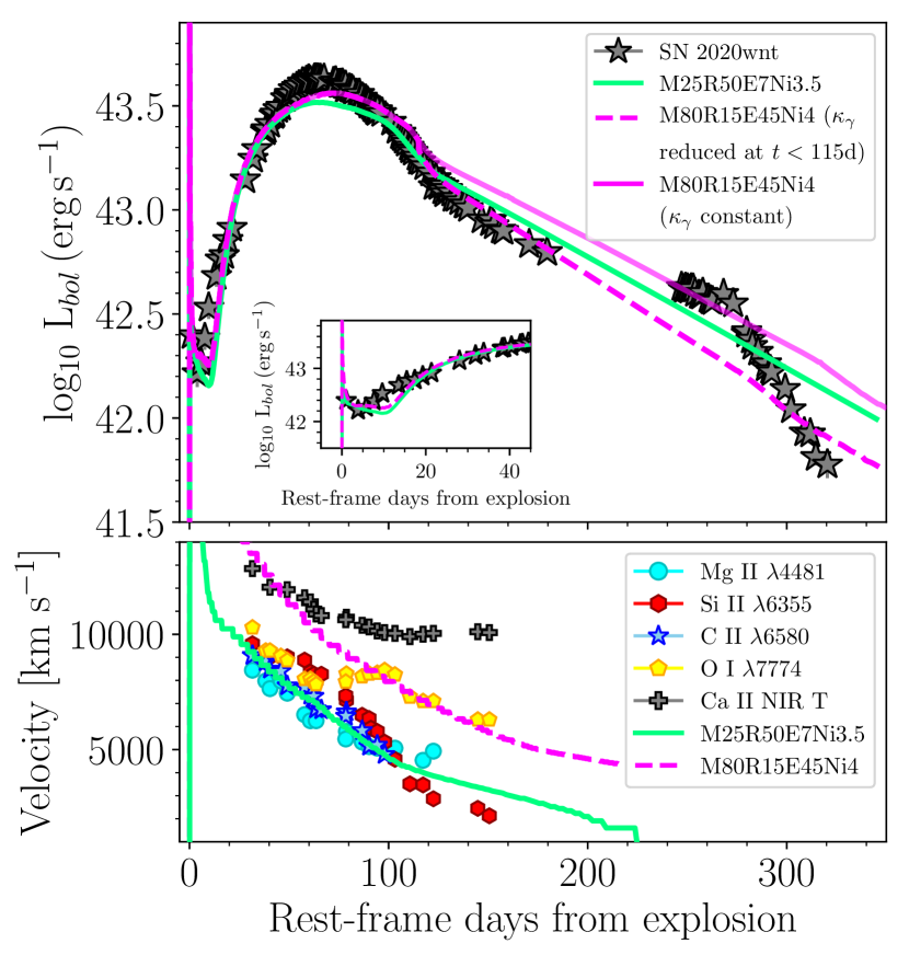
Figure 16: Top panel: Comparison between our best hydrodynamical models and the SN observations (grey stars). For the more massive model (magenta), we use a progenitor with a pre-SN mass of 80 M_⊙, $E_{\rm exp}=45\,\times 10^{51}$ erg, a ⁵⁶Ni mass of 4 M_⊙ and an initial radius of 15 R_⊙, while the less massive model (green solid line) has a a pre-SN mass of 25 M_⊙ and $E_{\rm exp}=7\,\times 10^{51}$ erg, a ⁵⁶Ni mass of 3.5 M_⊙ and an initial radius of 50 R_⊙. For the more massive model, we show the light curve with $\kappa_{\gamma}$ constant (solid line), and a light curve with $\kappa_{\gamma}$ reduction (dashed-line). The inset plot shows the light curves at very early phases. Bottom panel: Photospheric velocity of the models compared with the velocities of different species in SN 2020wnt.

To calculate the light curve and photospheric velocity, we use a one-dimensional local thermodynamical equilibrium (LTE) radiation hydrodynamical code presented in Bersten et al. (2011). The code follows the complete evolution of the light curve in a self-consistent way from the shock propagation to the nebular phase. The explosion initiates by injecting some energy near the progenitor core. This produces a powerful shock wave that propagates inside the progenitor until it arrives at the surface, where the photons begin to diffuse out. The code assumes a grey transport for gamma photons produced during the radioactive decay, but allows any distribution of this material inside the ejecta and assumes an opacity of $\kappa_{\gamma}=0.03$ cm² g^-1. Therefore, we are able to calculate the gamma-ray deposition in each part of the ejecta and estimate the gamma-ray escape as a function of time. The inclusion of a magnetar as an extra source to power the SN, including the relativistic effect, is accounted in the code (see Bersten et al., 2016, for details). An extensive exploration of magnetar parameters for different types of progenitors was discussed in Orellana et al. (2018).

An initial structure in hydrostatic equilibrium which simulates the condition of the star at the pre-SN stage is needed to start the hydrodynamical calculations. Here we assume both parametric and stellar evolutionary models. The initial emission and the rise time to the main peak of SN 2020wnt may indicate that a more extended progenitor is required than the typical stripped (or compact) star assumed for H-free objects. Therefore, we test models typically used for H-rich SNe with extended and dense envelopes like red supergiant (RSG) or blue supergiant (BSG) stars, but manually modifying the chemical abundance to produce a H-free envelope. The RSG models are computed by stellar evolutionary calculation while the BSG progenitor is computed assuming a double polytropic model given that it not easy to generate these BSG progenitors with stellar evolution models.

Assuming only a radioactive source, we cannot find a suitable solution for RSG (or stripped-envelope) progenitors, but models with a structure similar to those used for 87A-like objects or BSG progenitors (with our altered chemical composition) seem to offer a good solution. We generate several initial configurations for different values of the pre-SN mass (between 15 and 100 M_⊙) and radius (in the range of 15 to 80 R_⊙). We explore many values of the explosion energy and ⁵⁶Ni production for each configuration. Our best models are shown in the top panel of Figure 16 and correspond to two progenitors with a pre-SN radius of 50 and 15 R_⊙, pre-SN masses of 25 M_⊙ (green) and 80 M_⊙ (magenta), and explosion energies of $7\times 10^{51}$ erg and $45\times 10^{51}$ erg, respectively. In both cases, a large amount of ⁵⁶Ni (3.5 and 4 M_⊙) is required to reproduce the main peak of the light curve. For the more massive model (80 M_⊙), we slightly modified the gamma-ray opacity from $\kappa_{\gamma}=0.03$ to $\kappa_{\gamma}=0.013$ cm² g^-1 at around 115 days from the explosion to improve the fit from this epoch (i.e. allowing an easier leakage of gamma-ray photons; see Gutiérrez et al., 2021, for more details). However, we also include this model but with a $\kappa_{\gamma}$ constant (solid magenta line).

As observed in several SNe Ib/c (e.g. Sollerman et al., 2000, and references therein), the gamma-ray leakage significantly affects the light curve at late phases. More precisely, in several energetic SNe (e.g. SNe Ic broad line), the nickel mass required to explain the peak luminosity generally overestimates the tail luminosity (e.g. Maeda et al., 2003). To partially solve this issue, it has been proposed that an enhancement in the gamma-ray escape may happen in latter epochs (after the main peak). This could be due to possible asymmetries in the ejecta as the presence of low-density (or clumps) zones (Tominaga et al., 2005; Folatelli et al., 2006). Such types of structures could be produced by jets (e.g. Soker, 2022) or Rayleigh-Taylor instabilities. In these low-density regions, the gamma-rays could escape more efficiently, which can be simulated by reducing the kappa-gamma values. In addition, the grey transfer assumed for the gamma-rays can require a time varying factor, as shown in Wilk et al. (2019) by solving the relativistic radioactive transfer equation for gamma-ray in SNe.

The photospheric velocities of the models are compared to the velocities of different species in the bottom panel of Figure 16. The less massive model (25 M_⊙) reproduces the observables exceptionally well, particularly for Mg ii, Si ii and C ii; however, this is not the case for the 80 M_⊙ model. This model overestimates most of the velocities but has a good agreement with O i from 100 to 160 days.

Regarding the light curve, we found that the early emission can be attributed to the cooling phase for an extended progenitor of $\sim 50$ and 15 R_⊙, respectively. However, none of the models can reproduce the luminosity at phases later than $\sim 245$ days, since the hypotheses used in the code fail at these late times. At these epochs, the luminosity declines slower than the ⁵⁶Co decay (for about 30 days) and then suddenly drops. Between $\sim 245$ and $\sim 275$ days, the excess in luminosity is probably due to CSM interaction, which could be supported by the presence of H emission lines (H$\alpha$ and H$\beta$) in the late spectra (see Sections 3.4). The sudden drop in luminosity may be explained by the end of this interaction phase or alternative by dust formation. When the SN reaches the minimum value in this decrease, it almost recovers the luminosity expected from radioactivity (80 M_⊙ model). Ignoring these late epochs, the 25 and 80 M_⊙ models well describe the overall light curve evolution. Considering the photospheric velocities, the 25 M_⊙ model better represents the observed properties of SN 2020wnt. However, given the large amount of ⁵⁶Ni (3.5 M_⊙), this model turns out to be unrealistic. Relaxing the velocity constraints and considering that reaching an $E\geq 10^{52}$ requires a much higher and possibly nonphysical neutrino deposition fraction (Janka, 2012; Terreran et al., 2017), we find that the 80 M_⊙ model reproduces the light curve properties of SN 2020wnt very well. Additionally, given that t${}_{neb}\approx\sqrt{\kappa*M/v^{2}}\approx M*\sqrt{\kappa/E_{kin}}$ and t${}_{peak}\approx\sqrt{\kappa*M/(v*c)}$, we have t${}_{neb}^{2}\approx t_{peak}^{2}*c/v$. Since t_peak is fixed and our more massive model has higher velocities than the less massive model, the former is more compatible with the expected values for t_neb. Therefore, SN 2020wnt is consistent with a massive progenitor (pre-SN mass of 80 M_⊙), with a radius of 15 R_⊙, explosion energy of $45\times 10^{51}$ erg, and 4 M_⊙ of ⁵⁶Ni. These characteristics are compatible with the PISNe scenario (e.g. Gal-Yam et al. 2009; Kozyreva et al. 2014, but see Dessart et al. 2013).

As mentioned above, we also analyse the possibility that SN 2020wnt is powered by a magnetar. For this, we apply a version of our one-dimensional LTE radiation hydrodynamics code that takes into account the power provided by a newborn magnetar that loses rotational energy. That energy is fully deposited in the inner zones of the ejecta. We use the $\dot{E}$ vacuum prescription that became popular after the work of Kasen & Bildsten (2010) with the standard assumption of a magnetic dipole and a breaking index $n=3$. Modern and detailed treatments by Vurm & Metzger (2021) indicate that this approach is roughly valid at early times from the explosion. The parameters of this source are the surface magnetic field strength $B$ and the initial rotation period $P$.

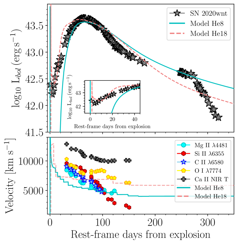
Figure 17: Top panel: Comparison between the magnetar models and the SN observations (grey stars). For the compact configuration (cyan solid line), we use a progenitor with a pre-SN mass of 8 M_⊙, $E_{\rm exp}=1\,\times 10^{51}$ erg and a magnetar with an initial period $P\sim 4.2$ ms and a magnetic field $B\sim 2\times 10^{14}$ G. In a more extended configuration (pink dashed-line), we use a progenitor with a pre-SN mass of 18 M_⊙, $E_{\rm exp}=1\,\times 10^{51}$ erg, $P\sim 2$ ms and a magnetic field $B\sim 3\times 10^{14}$ G. The inset plot shows the light curves at very early phases. Bottom panel: Photospheric velocity of the magnetar models compared with the velocities of different species in SN 2020wnt.

We test some of the H-poor progenitors, with a usual radioactive content of around 0.1 M_⊙. For the compact configuration ($M=8$ M_⊙ with $R=1.3$ R_⊙ and an explosion energy of $E_{\rm exp}=1\,\times 10^{51}$ erg ) the $L_{\text{peak}}$ of SN 2020wnt can be reached with $P\sim 4.2$ ms and $B\sim 2\times 10^{14}$ G, but the rise and post peak are not well reproduced (see Figure 17). We explore the same configuration with the mixing of the ⁵⁶Ni up to a fraction of 0.95 of the ejecta, but that makes no major changes. Then, we explore the possibility of a magnetar being applied to a more extended RSG structure. We use the results from Orellana et al. (2018) to select a possible model for SN 2020wnt. In Figure 17, we present the results for a progenitor with a pre-SN mass of 18 M_⊙ and a radius of 725 R_⊙. In this case the H is converted to He artificially, to have an inflated structure for a H-free star, though it is not the result of stellar evolution calculations. In order to obtain the time scale and the energy of the peak, the following magnetar parameters are required: $P\sim 2$ ms and $B\sim 3\times 10^{14}$ G, assuming an explosion energy of $E_{\rm exp}=1\,\times 10^{51}$ erg. While this model provides an improvement with respect to the compact model, it produces a worse representation of the light curve than the ⁵⁶Ni powered models presented in Figure 16. Additionally, the velocities are not well reproduced. Therefore, this result disfavours a magnetar model to explain the overall light curve evolution of SN 2020wnt.

We remark that none of the light curve models presented here is designed to fit the drastic drop in brightness observed from 273 days. Finally, although the ⁵⁶Ni powered models presented in Figure 16 provide a good explanation of SN 2020wnt for both the light curve and the velocities, the progenitor models used were built parametrically (both the pre-SN density profile and the chemical composition). It would be desirable to investigate what kind of evolutionary path, if any, can generate this type of structure to provide a more solid physical framework for our modelling.

5.3 CSM interaction

Despite the spectra of SN 2020wnt show remarkable similarities with SN 2007gr and non-interacting SNe Ic, the light curve fluctuations and the very high luminosity can be comfortably explained with the powering of ejecta-CSM interaction. Under this premise, we could consider that the actual ⁵⁶Ni-powered SN light curve would be below the observed one (similar to that observed for several SNe Ic; see top panel of Figure 13) dominated by ejecta-CSM interaction. We use TigerFit (Chatzopoulos et al., 2016; Wheeler et al., 2017) to explore this scenario by assuming a steady-state wind and a constant-density CSM shell, respectively. Although none of the fits reproduces the observed light curve of SN 2020wnt, we found that a steady-state wind CSM can reach a better approximation. In this context, a potentially pervasive interaction phase lasts for $\sim 273$ days and ends when the luminosity suddenly drops. Here, the CSM is probably H and He free. After the drop in brightness, the light curves continue to experience small fluctuations (see Figure 2), most likely attributed to episodes of CSM interaction. We note that very massive stars (M${}_{ZAMS}\sim 100-140$ M_⊙; Heger et al. 2003) are expected to lose mass through pulsational pair-instability. The SN ejecta are then expected to interact with the CSM gathered through former mass-loss events. This would generate luminous light curves, which may also show large luminosity fluctuations. Even though this scenario could reproduce the observable properties of SN 2020wnt, we do not have a model to test it.

6 Discussion

Similar pre-peak bump light curves have been detected in several SNe, which include SLSNe-I SN 2006oz, LSQ14bdq, DES14X3taz, DES15S2nr, DES17X1amf, SN 2018bsz and some signs of it in SN 2018hti (Fiore et al., 2022), and the peculiar SNe Ib/c SN 2005bf (Anupama et al., 2005; Tominaga et al., 2005; Folatelli et al., 2006; Maeda et al., 2007), PTF11mnb (Taddia et al., 2018a), and SN 2019cad (Gutiérrez et al., 2021). These bumps have been suggested to be a common characteristic of the SLSN class (Nicholl et al., 2016b), although more recent analyses with larger samples determined that such feature is not ubiquitous to all SLSNe-I (Angus et al., 2019).

Based on the analysis and comparison presented in previous sections, we found that SN 2020wnt is an object that seems to connect SN Ic and SLSN-I events. Although this connection was established before (e.g., Pastorello et al., 2010), the excellent photometric and spectroscopic coverage of this SN provides important insights to better understand such relations, and the implications for the explosion and progenitor stars. We discuss below the consequences of these results.

6.1 Unusual light curve evolution

As discussed in previous sections, the light curves of SN 2020wnt show remarkable features such as a pre-peak bump, a tail resembling the ⁵⁶Co decay followed by a sudden drop and minor luminosity fluctuations. Bumpy light curves have been observed before maximum in several SLSNe-I, as shown in Figure 10, and have been suggested to be frequent in the SLSN class (Nicholl et al., 2016b). However, more recent analyses with larger samples determined that such feature is not ubiquitous in SLSN-I (Angus et al., 2019). Early bumps have been interpreted as resulting from the recombination wave in the ejecta (Leloudas et al., 2012, for SN 2006oz), the shock breakout within a dense CSM (Moriya & Maeda, 2012), the shock cooling of extended material around the progenitor (Nicholl et al., 2015b; Piro, 2015; Smith et al., 2016; Angus et al., 2019) or an enhanced magnetar-driven shock breakout (Kasen et al., 2016). In the case of SN 2020wnt, we propose that such a feature is a consequence of a post-shock cooling phase in an extended progenitor (Section 5.2).

On the other hand, tails resembling the ⁵⁶Co decay have also been previously observed in other SLSNe-I, however, it was suggested that they may be powered by magnetar energy injection rather than ⁵⁶Co decay (Inserra et al. 2013, but see Gal-Yam 2012). In the case of SN 2020wnt, and as shown in Section 5.2, the ⁵⁶Ni models provide a better representation of the light curve of SN 2020wnt than those obtained with the magnetar model, suggesting that the main source of power is radioactivity. Signs of CSM interaction (e.g. presence of H lines in the spectra, light curve fluctuations) may imply additional energy contribution from the CSM interaction.

Starting from 273 days from explosion, SN 2020wnt shows a sudden drop in brightness. Although resembling breaks have been observed in a few SLSNe I (e.g. Inserra et al., 2017), several interacting objects (e.g. Mattila et al., 2008; Pastorello et al., 2008; Ofek et al., 2014; Tartaglia et al., 2020), and in some Super-Chandrasekhar SNe Ia (e.g. Hsiao et al., 2020), the slope measured in SN 2020wnt is unique. While for slow-evolving SLSNe I, Inserra et al. (2017) measured a decline that follows a power law of $t^{-5}$, interacting objects and Super-Chandrasekhar SNe Ia usually show less steep declines (e.g. Fransson et al., 2014; Moriya, 2014). On the contrary, for SN 2020wnt, we find a much steeper slope, which follows a power law of $t^{-11}$.

It has been discussed that this break can either be caused by the breakout of the shock through the dense shell (Ofek et al., 2014; Fransson et al., 2014), or the result of a transition to a momentum-conserving phase, occurring when shock runs over a mass of CSM equivalent to the ejecta mass (Ofek et al. 2014, but see Moriya 2014), or the result of CO formation (Hsiao et al., 2020), or even the consequence of dust formation in a cool, dense shell (Pastorello et al., 2008; Mattila et al., 2008; Smith et al., 2008). Despite the breakout of the shock through the dense shell being a plausible explanation for a type IIn event such as SN 2010jl, it is less reliable for SN 2020wnt. While SN 2020wnt shows some signatures of interaction, its spectra lack flat-topped profiles and intermediate-width features, which are expected from the interaction of the ejecta with dense CSM. However, as mentioned in Section 5, ejecta-CSM interaction may play an important role in the sudden drop observed in the late optical light curve of SN 2020wnt. Although CO and dust formation could be an option, it is not supported by the spectrum at 293 days from explosion (taken during the early part of the sudden drop). Here, we do not detect any emission line blueshifted, typically seen in SN spectra with dust forming in the ejecta. However, to confirm or reject this alternative, NIR observations are needed.

6.2 Absence of O ii lines and presence of C ii lines

One of the most common features observed in the early phase spectra of SLSNe-I is the presence of O ii lines around 4000 – 4500 Å (Quimby et al. 2011, 2018; but see, Könyves-Tóth & Vinkó 2021). These lines appear at high temperatures (12000-15000 K; Inserra 2019) as a consequence of non-thermal excitation (Mazzali et al., 2016). In the case of SN 2020wnt, we noticed that these lines are not visible in the spectra at any epoch (see Figure 4). As shown in Section 3.3 (and Figure 3), the temperature of SN 2020wnt evolves in a range of values lower than 10000 K. This temperature is indeed not high enough to ionise the oxygen. Quimby et al. (2018) suggested that the lack of these features, at least in standard luminosity SNe Ic, may be either the product of rapid cooling or due to a lack of non-thermal sources of excitation. Given that the initial emission can be reproduced as the results of the cooling of an extended progenitor, this is not compatible with a rapid cooling phase. Therefore, the lack of a non-thermal source seems to be the most reliable explanation. This is also supported by our modelling, which does not require a very extended mixing of radioactive material.

Gal-Yam (2019) found that, in addition to the O lines, the C lines are also typical of SLSNe I at around peak, and suggested that they result from the emission of an almost pure C/O envelope, without significant contamination of higher-mass elements from deeper layers. Inspecting the spectra of SN 2020wnt, we detect strong and persistent lines of C ii. These lines are predicted by spectral models (Dessart et al., 2012; Mazzali et al., 2016; Dessart, 2019), and are identified in several SLSNe-I (e.g., PTF09cnd (Quimby et al., 2018), PTF10aagc (Quimby et al., 2018), PTF12dam, SN 2015bn, Gaia16apd (Yan et al., 2017a), iPFT16bad (Yan et al., 2017b), SN 2017gci, SN 2018bsz, SN 2018hti (Lin et al., 2020; Fiore et al., 2022), although in most of the cases, the strength of the lines is moderate. However, SN 2020wnt along with SN 2018bsz, have stronger lines than these other objects, and furthermore their C ii lines agree with the models of Dessart (2019), which typically overestimate the observed strength of these lines.

In the spectra of SN 2020wnt, we also detect a strong Si ii. A weak Si ii feature has been detected in a few objects (e.g. PTF09cnd and SN 2015bn). From the modelling side, Si ii is not predicted by the models presented in Mazzali et al. (2016), but it is reproduced by the magnetar model presented in Dessart et al. (2012). They argue that the presence of the Si ii, C ii, and He i lines is a result of the extra energy from a magnetar that heats the material and thermally excites the gas. Although the detection of these lines in SN 2020wnt supports this scenario, our light curve modelling (Section 5.2) disfavours it.

6.3 SN 2020wnt: an extreme case of SN 2007gr?

As discussed before (Section 4.3), the spectral evolution of SN 2020wnt resembles that of the carbon-rich type Ic SN 2007gr. In Section 4, we showed that their light curves evolve differently. Indeed, SN 2020wnt is over 3 magnitudes brighter than SN 2007gr, it evolves much more slowly (it is $\sim 4$ times slower) and has the pre-peak bump that was not detected in its fainter counterpart. However, the remarkable similarity of the spectra suggests that they may have a progenitor with a similar composition. The question that arises from this comparison is why SN 2020wnt and SN 2007gr show comparable spectroscopic behaviour but completely different photometric properties?

In our attempt to provide an answer, we analyse the environments of these objects. In Section 3.1 we mentioned that SN 2020wnt is in a metal-poor environment (12 + log(O/H)$=8.175$ dex by using the mass-metallicity relation of Kewley & Ellison 2008). More precisely, its host galaxy is faint, has a low stellar mass and very little star formation, similar to those observed for SLSNe-I. On the other hand, the host of SN 2007gr was identified as a nearby spiral galaxy (M${}_{B}=-18.89$; Makarov et al. 2014) that also hosted SN 1969L and SN 1961V (Hunter et al., 2009; Chen et al., 2014). According to Maund & Ramirez-Ruiz (2016), SN 2007gr was located at near the centre of a dense young, massive star association (Kuncarayakti et al., 2013). Modjaz et al. (2011) measured the metallicity near the position of SN 2007gr by using the O3N2 diagnostic method (Pettini & Pagel, 2004) and found it was 12 + log(O/H)$=8.64$ dex, indicating a metal-rich environment. These results lead us to conclude that the host environments of SN 2020wnt and SN 2007gr are different, and based on these estimations, also the metallicity of their progenitor stars.

The nature of the progenitor star and explosion of SN 2007gr has been broadly discussed (e.g., Crockett et al., 2008; Chen et al., 2014; Maund & Ramirez-Ruiz, 2016). Chen et al. (2014) suggested that the progenitor of SN 2007gr was a low-mass Wolf–Rayet star resulting from an interacting binary. Maund & Ramirez-Ruiz (2016) support a Wolf–Rayet progenitor, but add that it was an initially massive star. From the nebular modelling, Mazzali et al. (2010) found that SN 2007gr was the explosion of a low-mass CO core, probably the result of a star with an initial mass of 15 M_⊙. For SN 2020wnt, our light curve modelling suggests a massive progenitor and an energetic explosion with lot of ⁵⁶Ni produced. These parameters are, in all respects, more extreme than those found for SN 2007gr.

7 Conclusions

SN 2020wnt is a slow-evolving carbon-rich SLSN-I. Its light curves show an early bump lasting $\sim 5$ days followed by a slow rise to the main peak. The peak is reached at different times, occurring faster in the bluer bands. With an absolute peak magnitudes of around $\sim-20.5$ mag, SN 2020wnt is in the low end of the luminosity distribution of SLSNe-I. After 130 days from explosion, the light curves show a linear decline in all bands, with slopes being around the expected decline rate of the ⁵⁶Co decay. Later, from 273 days, a sudden drop in brightness is observed, implying a significant leakage of gamma-ray photons. Our last observations (after 350 days from explosion), show an increase in brightness, which may suggest interaction between the ejecta and the CSM. Indeed, minor light curve fluctuations support this scenario.

During the photospheric phase, the optical spectra show clear lines of C ii and Si ii, while the classical O ii lines that typically characterise SLSNe-I are not detected. The lack of O ii lines is probably related to the low temperatures of this object (below 10000 K). Late-time spectra display strong lines of [O i], [Ca ii], Ca ii, Mg i], as well as, a broad emission of [O iii] and Balmer lines.

We modelled the light curve and the expansion velocities of SN 2020wnt using a one-dimensional hydrodynamics code. Two scenarios were investigated, with the radioactive nickel and the magnetar as primary powering sources. In both cases, we found that an extended progenitor was required to reproduce the time scale of the peaks. However, the magnetar model produces a much worse fit to the data. Therefore, we consider the ⁵⁶Ni as the main power source. Specifically, we found that SN 2020wnt can be explained by a progenitor with a pre-SN mass of 80 M_⊙, a pre-SN radius of 15 R_⊙, an explosion energy of $45\times 10^{51}$ erg, and ejecting 4 M_⊙ of ⁵⁶Ni. In this scenario, the first peak results from a post-shock cooling phase for the extended progenitor, and the luminous main peak is due to a large ⁵⁶Ni production. The values of the parameters obtained are consistent with those expected for a PISN, which provide support for this scenario in the case of SN 2020wnt. Although our model reproduces the almost complete evolution of the light curve reasonably well, it fails to explain the excess of flux at $\sim 245$ days and the shape of the light curve after that. We propose that this behaviour is probably due to an additional contribution of ejecta-CSM interaction. The drop in brightness after 273 days from explosion could be attributed to either the end of earlier ejecta-CSM interaction, or the formation of molecules and dust in the SN ejecta or in a shocked cool dense shell. However, NIR observation are needed to confirm this suggestion.

We noticed remarkable spectral similarities between SN 2020wnt and carbon-rich type Ic SN 2007gr, but on a longer time scale. This resemblance may suggest a connection between these two events, most probably associated with the structures of their progenitor stars. Although we have found a model that can explain the main photometric properties of SN 2020wnt, we also discussed a possibility where the CSM interaction is the primary energy source already at early phases. However, we did not explore in detail this alternative scenario due to the lack of an available model with such extreme input parameters as those observed in SN 2020wnt.

Data Availability

The data underlying this article are available in the appendix A (Tables A1 – A5) and through the WISeREP (https://wiserep.weizmann.ac.il/home) archive (Yaron & Gal-Yam, 2012).

Supporting information

Supplementary data are available at MNRAS online.

Table A1. Optical photometry of SN 2020wnt.
Table A2. JHK Vega photometry of SN 2020wnt obtained with NOTCam.
Table A3. UV photometry obtained with Swift in the AB system.
Table A4. ATLAS AB optical photometry.
Table A5. ZTF AB optical photometry.
Table A6. Spectroscopic observations of SN 2020wnt.

Appendix A Tables

Table A1: Optical photometry of SN 2020wnt.

UT date	MJD	Phase	$u$	$B$	$V$	$g$	$r$	$i$	$z$	Telescope
		(days)∗	(mag)	(mag)	(mag)	(mag)	(mag)	(mag)	(mag)
20201121	59174.83	38.21	$18.43\pm 0.14$	$17.91\pm 0.05$	$17.28\pm 0.03$	$17.57\pm 0.03$	$17.11\pm 0.03$	$16.94\pm 0.06$	–	Schmidt Telescope
20201121	59174.99	38.36	$18.40\pm 0.03$	$17.93\pm 0.02$	$17.25\pm 0.01$	$17.50\pm 0.01$	$17.07\pm 0.01$	$16.92\pm 0.01$	$16.87\pm 0.02$	Copernico 1.82-m
20201124	59177.13	40.44	$18.38\pm 0.10$	$17.84\pm 0.04$	$17.16\pm 0.03$	$17.44\pm 0.03$	$17.01\pm 0.03$	$16.84\pm 0.04$	–	Schmidt Telescope
20201126	59179.84	43.06	–	$17.67\pm 0.06$	$17.05\pm 0.06$	$17.37\pm 0.07$	$16.86\pm 0.07$	$16.73\pm 0.07$	–	Schmidt Telescope
20201129	59182.83	45.96	–	$17.63\pm 0.07$	$16.94\pm 0.06$	$17.28\pm 0.11$	$16.81\pm 0.05$	$16.69\pm 0.06$	–	Schmidt Telescope
20201203	59186.97	49.97	$18.01\pm 0.02$	$17.44\pm 0.02$	$16.83\pm 0.01$	$17.08\pm 0.01$	$16.66\pm 0.01$	$16.49\pm 0.01$	$16.47\pm 0.01$	LT
20201205	59188.01	50.98	$17.98\pm 0.02$	–	–	$17.03\pm 0.01$	$16.64\pm 0.01$	$16.46\pm 0.01$	$16.50\pm 0.02$	LT
20201207	59190.97	53.85	$17.89\pm 0.02$	$17.34\pm 0.01$	$16.72\pm 0.01$	$16.93\pm 0.01$	$16.54\pm 0.01$	$16.37\pm 0.01$	$16.35\pm 0.01$	LT
20201210	59193.97	56.75	$17.84\pm 0.02$	$17.28\pm 0.01$	$16.66\pm 0.01$	$16.87\pm 0.01$	$16.49\pm 0.01$	$16.28\pm 0.01$	$16.28\pm 0.01$	LT
20201212	59195.97	58.69	$17.80\pm 0.17$	$17.23\pm 0.03$	$16.68\pm 0.16$	$16.94\pm 0.05$	$16.46\pm 0.03$	$16.33\pm 0.03$	$16.22\pm 0.04$	LT
20201213	59196.09	58.81	–	$17.25\pm 0.14$	$16.67\pm 0.03$	$16.91\pm 0.03$	$16.47\pm 0.07$	$16.39\pm 0.07$	–	Schmidt Telescope
20201213	59196.97	59.66	$17.82\pm 0.02$	$17.24\pm 0.01$	$16.60\pm 0.01$	$16.87\pm 0.01$	$16.44\pm 0.01$	$16.28\pm 0.03$	$16.24\pm 0.01$	LT
20201214	59197.98	60.64	–	$17.26\pm 0.04$	$16.66\pm 0.03$	$16.90\pm 0.03$	$16.47\pm 0.04$	$16.35\pm 0.04$	–	Schmidt Telescope
20201216	59199.88	62.48	–	–	–	$16.86\pm 0.01$	$16.47\pm 0.01$	$16.33\pm 0.02$	$16.23\pm 0.02$	Copernico 1.82-m
20201216	59199.95	62.55	–	$17.24\pm 0.01$	$16.60\pm 0.01$	–	–	–	–	LT
20201217	59200.95	63.52	$17.82\pm 0.02$	$17.25\pm 0.01$	$16.58\pm 0.02$	$16.84\pm 0.01$	$16.41\pm 0.01$	$16.20\pm 0.01$	$16.20\pm 0.01$	LT
20201218	59201.92	64.46	–	$17.27\pm 0.05$	$16.65\pm 0.03$	$16.91\pm 0.02$	$16.46\pm 0.03$	$16.23\pm 0.05$	–	Schmidt Telescope
20201218	59201.94	64.48	$17.83\pm 0.02$	$17.25\pm 0.02$	$16.60\pm 0.03$	$16.84\pm 0.01$	$16.43\pm 0.00$	$16.20\pm 0.01$	$16.18\pm 0.01$	LT
20201220	59203.75	66.23	$17.87\pm 0.03$	$17.24\pm 0.03$	$16.62\pm 0.02$	$16.88\pm 0.02$	$16.48\pm 0.03$	$16.24\pm 0.01$	$16.22\pm 0.02$	Copernico 1.82-m
20201227	59210.04	72.33	$18.04\pm 0.03$	–	–	$16.87\pm 0.01$	$16.39\pm 0.01$	$16.18\pm 0.01$	$16.13\pm 0.01$	NOT
20201229	59212.68	74.88	–	–	$16.69\pm 0.22$	–	$16.35\pm 0.06$	$16.03\pm 0.18$	–	TNT
20201230	59213.66	75.83	–	–	$16.62\pm 0.14$	$16.85\pm 0.06$	$16.35\pm 0.07$	$16.15\pm 0.12$	–	TNT
20201231	59214.69	76.83	–	$17.31\pm 0.03$	$16.59\pm 0.10$	$16.83\pm 0.04$	$16.35\pm 0.05$	$16.18\pm 0.10$	–	TNT
20210101	59215.02	77.15	–	$17.27\pm 0.15$	$16.62\pm 0.07$	$16.88\pm 0.06$	$16.43\pm 0.04$	$16.18\pm 0.03$	$16.19\pm 0.05$	LT
20210101	59215.95	78.05	–	–	$16.64\pm 0.23$	–	$16.44\pm 0.16$	$16.18\pm 0.19$	–	LT
20210105	59219.47	81.46	–	$17.42\pm 0.02$	$16.59\pm 0.01$	$16.94\pm 0.01$	$16.39\pm 0.05$	$16.20\pm 0.01$	–	TNT
20210109	59223.45	85.32	–	$17.49\pm 0.03$	$16.60\pm 0.02$	$16.98\pm 0.04$	$16.40\pm 0.01$	$16.18\pm 0.01$	–	TNT
20210110	59224.96	86.78	–	$17.51\pm 0.02$	$16.70\pm 0.02$	$17.09\pm 0.02$	$16.51\pm 0.02$	$16.18\pm 0.01$	$16.14\pm 0.01$	Copernico 1.82-m
20210112	59226.65	88.42	–	$17.66\pm 0.02$	$16.67\pm 0.03$	$17.12\pm 0.03$	$16.47\pm 0.02$	$16.25\pm 0.02$	–	TNT
20210113	59227.55	89.29	–	$17.66\pm 0.02$	$16.70\pm 0.02$	$17.19\pm 0.02$	$16.43\pm 0.02$	$16.23\pm 0.02$	–	TNT
20210114	59228.05	89.78	–	$17.67\pm 0.02$	$16.72\pm 0.02$	$17.15\pm 0.02$	$16.47\pm 0.02$	$16.20\pm 0.01$	–	Schmidt Telescope
20210115	59229.59	91.27	–	$17.74\pm 0.02$	$16.75\pm 0.02$	$17.22\pm 0.03$	$16.50\pm 0.02$	$16.24\pm 0.02$	–	TNT
20210116	59230.63	92.28	–	$17.84\pm 0.02$	$16.78\pm 0.02$	$17.25\pm 0.03$	$16.51\pm 0.02$	$16.26\pm 0.01$	–	TNT
20210117	59231.59	93.21	–	$17.89\pm 0.02$	$16.82\pm 0.02$	$17.31\pm 0.02$	$16.54\pm 0.02$	$16.30\pm 0.02$	–	TNT
20210117	59231.86	93.47	–	$17.83\pm 0.02$	$16.83\pm 0.02$	$17.30\pm 0.02$	$16.54\pm 0.03$	$16.23\pm 0.02$	–	Schmidt Telescope
20210118	59232.81	94.39	$18.87\pm 0.04$	$17.84\pm 0.02$	$16.85\pm 0.02$	$17.35\pm 0.01$	$16.56\pm 0.01$	$16.28\pm 0.01$	$16.18\pm 0.01$	Copernico 1.82-m
20210120	59234.86	96.38	$19.06\pm 0.05$	$17.98\pm 0.02$	$16.85\pm 0.03$	$17.41\pm 0.02$	$16.52\pm 0.02$	$16.26\pm 0.04$	$16.11\pm 0.02$	NOT
20210125	59239.95	101.31	$19.41\pm 0.07$	$18.21\pm 0.02$	$16.95\pm 0.01$	$17.57\pm 0.01$	$16.57\pm 0.01$	$16.25\pm 0.01$	$16.15\pm 0.01$	LT
20210128	59242.75	104.02	–	$18.31\pm 0.06$	$17.01\pm 0.02$	$17.67\pm 0.03$	$16.66\pm 0.02$	$16.29\pm 0.02$	–	Schmidt Telescope
20210130	59244.57	105.78	–	$18.40\pm 0.02$	$17.15\pm 0.02$	$17.78\pm 0.03$	$16.68\pm 0.02$	$16.40\pm 0.02$	–	TNT
20210130	59244.94	106.14	$19.77\pm 0.10$	$18.40\pm 0.03$	$17.10\pm 0.01$	$17.76\pm 0.02$	$16.68\pm 0.01$	$16.31\pm 0.01$	$16.23\pm 0.01$	LT
20210131	59245.56	106.74	–	$18.33\pm 0.02$	$17.18\pm 0.02$	$17.81\pm 0.03$	$16.75\pm 0.02$	$16.44\pm 0.02$	–	TNT
20210201	59246.54	107.69	–	$18.49\pm 0.02$	$17.16\pm 0.02$	$17.86\pm 0.03$	$16.76\pm 0.02$	$16.46\pm 0.02$	–	TNT
20210202	59247.58	108.70	–	$18.56\pm 0.02$	$17.21\pm 0.02$	$17.92\pm 0.03$	$16.82\pm 0.02$	$16.50\pm 0.02$	–	TNT
20210204	59249.78	110.83	–	$18.67\pm 0.01$	$17.39\pm 0.08$	$18.13\pm 0.13$	$16.90\pm 0.05$	$16.56\pm 0.03$	–	Schmidt Telescope
20210208	59253.86	114.79	–	–	$17.52\pm 0.02$	$18.31\pm 0.03$	$17.13\pm 0.03$	$16.76\pm 0.16$	$16.55\pm 0.03$	Copernico 1.82-m
20210216	59261.87	122.55	$21.19\pm 0.09$	$19.52\pm 0.02$	$17.89\pm 0.01$	$18.78\pm 0.01$	$17.44\pm 0.01$	$17.05\pm 0.01$	$16.76\pm 0.01$	NOT
20210219	59264.48	125.08	–	$19.49\pm 0.02$	$18.07\pm 0.02$	$18.75\pm 0.03$	$17.51\pm 0.02$	$17.09\pm 0.09$	–	TNT
20210219	59264.75	125.34	–	–	$18.15\pm 0.06$	–	$17.63\pm 0.06$	$17.14\pm 0.03$	–	Schmidt Telescope
20210220	59265.81	126.37	–	$19.75\pm 0.15$	–	$18.89\pm 0.11$	–	–	–	Schmidt Telescope
20210221	59266.48	127.02	–	$19.50\pm 0.02$	$18.17\pm 0.02$	$18.89\pm 0.03$	$17.55\pm 0.02$	$17.18\pm 0.02$	–	TNT
20210222	59267.46	127.97	–	$19.67\pm 0.02$	$18.20\pm 0.02$	$19.08\pm 0.03$	$17.58\pm 0.02$	$17.25\pm 0.02$	–	TNT
20210226	59271.77	132.14	–	–	$18.30\pm 0.05$	–	$17.77\pm 0.04$	$17.33\pm 0.07$	–	Schmidt Telescope
20210228	59273.77	134.08	–	–	–	$19.17\pm 0.13$	–	–	–	Schmidt Telescope
20210304	59277.53	137.72	–	$19.74\pm 0.02$	$18.33\pm 0.07$	$19.13\pm 0.22$	$17.70\pm 0.02$	$17.26\pm 0.02$	–	TNT
20210306	59279.80	139.92	–	–	$18.37\pm 0.05$	–	$17.80\pm 0.04$	$17.39\pm 0.03$	–	Schmidt Telescope
20210313	59286.79	146.70	–	–	–	–	$17.90\pm 0.05$	$17.41\pm 0.02$	$17.06\pm 0.03$	Copernico 1.82-m
20210318	59291.86	151.61	$21.65\pm 0.25$	$20.00\pm 0.02$	$18.36\pm 0.01$	$19.19\pm 0.04$	$17.87\pm 0.01$	$17.41\pm 0.01$	$17.01\pm 0.01$	NOT
20210323	59296.79	156.39	–	–	–	–	$17.96\pm 0.05$	$17.55\pm 0.04$	–	Schmidt Telescope
20210407	59311.49	170.63	–	–	–	–	$18.06\pm 0.25$	$17.74\pm 0.07$	–	TNT
20210416	59320.81	179.66	–	–	–	–	$18.18\pm 0.08$	$17.82\pm 0.05$	–	Schmidt Telescope
20210628	59393.07	249.68	–	–	–	–	–	$18.46\pm 0.10$	–	Schmidt Telescope
20210630	59395.08	251.63	–	–	–	$19.47\pm 0.27$	–	–	–	Schmidt Telescope
20210701	59396.06	252.58	–	–	–	$19.44\pm 0.14$	–	–	–	Schmidt Telescope
20210706	59401.06	257.83	–	$20.29\pm 0.19$	–	–	–	–	–	Schmidt Telescope
20210707	59402.07	257.42	–	–	$19.13\pm 0.10$	–	–	–	–	Schmidt Telescope
20210708	59403.07	259.37	–	–	–	$19.81\pm 0.18$	–	$18.55\pm 0.08$	–	Schmidt Telescope
20210717	59412.22	268.24	$>20.87$	$20.37\pm 0.04$	$19.05\pm 0.05$	$19.50\pm 0.08$	$18.91\pm 0.03$	$18.53\pm 0.07$	$17.84\pm 0.05$	LT
20210722	59417.22	273.08	$>21.29$	$20.38\pm 0.04$	$19.22\pm 0.05$	$19.66\pm 0.06$	$18.97\pm 0.02$	$18.57\pm 0.11$	$17.97\pm 0.17$	LT
20210729	59424.05	279.70	–	–	–	–	$19.38\pm 0.11$	$19.23\pm 0.10$	–	Schmidt Telescope
20210729	59424.18	279.83	$>20.97$	$20.88\pm 0.08$	$19.53\pm 0.08$	$19.84\pm 0.08$	$19.36\pm 0.09$	$19.05\pm 0.09$	$18.32\pm 0.07$	LT
20210801	59427.21	282.76	$>21.66$	$21.15\pm 0.16$	$19.62\pm 0.04$	$20.16\pm 0.06$	$19.51\pm 0.06$	$19.18\pm 0.12$	$18.54\pm 0.13$	LT
20210804	59430.18	285.64	–	$21.00\pm 0.24$	$19.75\pm 0.06$	$20.31\pm 0.06$	$19.57\pm 0.09$	$19.22\pm 0.19$	$18.58\pm 0.13$	LT
20210808	59434.15	289.49	–	$21.18\pm 0.10$	$19.95\pm 0.10$	$20.48\pm 0.09$	$19.71\pm 0.11$	$19.43\pm 0.25$	$18.80\pm 0.17$	LT
20210811	59437.16	292.40	–	$21.19\pm 0.34$	$20.10\pm 0.11$	$20.63\pm 0.11$	$19.82\pm 0.07$	$19.62\pm 0.14$	$18.96\pm 0.18$	LT
20210814	59440.17	295.32	–	$21.56\pm 0.32$	$20.32\pm 0.38$	$20.68\pm 0.42$	$20.05\pm 0.59$	$19.71\pm 0.81$	$18.98\pm 0.41$	LT
20210818	59444.18	299.21	–	–	$20.15\pm 0.13$	$20.67\pm 0.13$	$19.97\pm 0.09$	$19.73\pm 0.11$	$19.33\pm 0.10$	LT
20210821	59447.19	302.12	–	–	$20.61\pm 0.15$	$21.07\pm 0.15$	$20.28\pm 0.15$	$19.87\pm 0.34$	$19.50\pm 0.21$	LT
20210828	59454.10	308.82	–	–	$20.67\pm 0.14$	$21.10\pm 0.24$	$20.57\pm 0.11$	$20.08\pm 0.25$	$19.77\pm 0.17$	LT

Table A1: – continued

UT date	MJD	Phase	$u$	$B$	$V$	$g$	$r$	$i$	$z$	Telescope
		(days)∗	(mag)	(mag)	(mag)	(mag)	(mag)	(mag)	(mag)
20210831	59457.19	311.81	–	–	$20.82\pm 0.10$	$21.33\pm 0.12$	$20.45\pm 0.28$	$20.07\pm 0.44$	$19.59\pm 0.30$	LT
20210903	59460.04	314.57	–	–	$21.10\pm 0.12$	–	$20.77\pm 0.15$	$20.48\pm 0.18$	$19.87\pm 0.16$	Copernico 1.82-m
20210909	59466.07	320.42	–	$22.05\pm 0.25$	$21.24\pm 0.25$	$21.62\pm 0.14$	$20.56\pm 0.20$	$20.55\pm 0.24$	$20.11\pm 0.27$	TNG
20211027	59514.94	367.77	–	–	–	$21.30\pm 0.06$	$20.55\pm 0.02$	$20.60\pm 0.07$	$19.95\pm 0.11$	NOT
20220227	59637.92	486.94	–	$22.33\pm 0.35$	$21.56\pm 0.25$	$21.85\pm 0.18$	$21.38\pm 0.18$	$21.18\pm 0.22$	$20.78\pm 0.15$	NOT

• Notes:
  ^∗ Rest-frame phase in days from explosion, MJD=$59135.42\pm 0.98$.
  $BV$ photometry is in the Vega system, while $ugriz$ photometry is in the AB system.
  Copernico 1.82-m: Copernico 1.82 m telescope at the Asiago Observatory (Italy). LT: 2-m Liverpool Telescope at the Observatorio del Roque de Los Muchachos (Spain). NOT: 2.56-m Nordic Optical Telescope at the Roque de Los Muchachos Observatory (Spain). Schmidt Telescope: 67/91 Schmidt Telescope at the Asiago Observatory (Italy). TNG 3.6-m Telescopio Nazionale Galileo at the Roque de Los Muchachos Observatory (Spain). TNT: 0.8-m Tsinghua University–NAOC (National Astronomical Observatories of China) Telescope at Xinglong Observatory of NAOC.

Table A2: $JHK$ Vega photometry of SN 2020wnt obtained with NOTCam.

UT date	MJD	Phase	J	H	K
		(days)∗	(mag)	(mag)	(mag)
20201216	59199.97	62.57	$15.54\pm 0.01$	$15.57\pm 0.01$	–
20210126	59240.36	101.71	$15.37\pm 0.01$	$15.08\pm 0.01$	$14.965\pm 0.01$
20210219	59264.43	125.03	$16.23\pm 0.03$	$15.71\pm 0.03$	$15.577\pm 0.02$
20210317	59290.39	150.18	$16.26\pm 0.03$	$15.80\pm 0.03$	$15.747\pm 0.12$
20210403	59307.40	166.67	$16.64\pm 0.04$	$15.95\pm 0.11$	$15.960\pm 0.12$
20210716	59411.40	267.44	$17.49\pm 0.04$	$16.76\pm 0.05$	$16.340\pm 0.05$
20210810	59436.31	291.58	$18.39\pm 0.07$	$17.77\pm 0.06$	$17.275\pm 0.11$
20211012	59499.15	352.47	$19.16\pm 0.12$	$18.38\pm 0.15$	$17.808\pm 0.19$
20211208	59556.30	407.85	$19.56\pm 0.20$	$18.68\pm 0.20$	$18.083\pm 0.15$
20220204	59614.40	464.15	$19.77\pm 0.19$	$19.00\pm 0.18$	$17.991\pm 0.13$

• Notes:
  ^∗ Rest-frame phase in days from explosion, MJD=$59135.42\pm 0.98$

Table A3: UV photometry obtained with Swift in the AB system.

UT date	MJD	Phase	UVW2	UVM2	UVW1	U	B	V
		(days)∗	(mag)	(mag)	(mag)	(mag)	(mag)	(mag)
20201123	59176.18	39.51	$22.12\pm 0.52$	$22.22\pm 0.56$	$19.95\pm 0.18$	$18.53\pm 0.13$	$17.82\pm 0.07$	$17.14\pm 0.09$
20210114	59228.42	90.14	$22.07\pm 0.50$	$>21.64$	$21.14\pm 0.43$	$18.62\pm 0.13$	$17.53\pm 0.08$	$16.59\pm 0.08$
20210203	59248.08	109.19	$23.21\pm 1.51$	$>21.43$	–	$20.58\pm 0.52$	$18.55\pm 0.09$	$17.16\pm 0.08$
20210223	59268.20	128.68	$22.47\pm 2.31$	$>19.89$	$21.99\pm 3.16$	$20.78\pm 1.61$	$19.41\pm 0.30$	$18.07\pm 0.26$
20210227	59272.37	132.73	$22.94\pm 0.96$	$>21.75$	–	–	–	–
20210303	59276.82	137.04	–	$>21.39$	$21.69\pm 0.76$	$21.07\pm 0.80$	$19.51\pm 0.22$	$18.25\pm 0.24$
20210315	59288.78	148.62	–	$>21.45$	–	$22.37\pm 2.56$	$20.32\pm 0.63$	$18.06\pm 0.26$
20210318	59291.03	150.80	$22.11\pm 1.16$	$>20.50$	$20.48\pm 0.57$	$20.65\pm 1.16$	$19.89\pm 0.23$	$18.29\pm 0.19$

• Notes:

• ^∗ Rest-frame phase in days from explosion, MJD=$59135.42\pm 0.98$.

Table A4: ATLAS AB optical photometry.

UT date	MJD	Phase	Band	Magnitude
		(days)∗		(mag)
20200926	59118.49	-16.386	$o$	$>22.71$
20201004	59126.48	-8.643	$o$	$>22.00$
20201014	59136.50	1.066	$c$	$19.70\pm 0.11$
20201018	59140.48	4.922	$c$	$20.05\pm 0.22$
20201020	59142.44	6.822	$o$	$19.61\pm 0.10$
20201022	59144.41	8.731	$c$	$19.61\pm 0.09$
20201024	59146.55	10.804	$o$	$19.02\pm 0.06$
20201026	59148.50	12.694	$o$	$18.70\pm 0.11$
20201026	59148.57	12.762	$c$	$19.70\pm 0.59$
20201028	59150.59	14.719	$o$	$18.65\pm 0.04$
20201031	59153.44	17.481	$o$	$18.52\pm 0.10$

Table A4: – continued

20201109	59162.46	26.221	$o$	$17.81\pm 0.02$
20201117	59170.48	33.992	$o$	$17.20\pm 0.02$
20201123	59176.41	39.738	$o$	$16.92\pm 0.04$
20201125	59178.48	41.744	$o$	$16.90\pm 0.01$
20201127	59180.42	43.624	$o$	$16.86\pm 0.02$
20201202	59185.47	48.517	$o$	$16.66\pm 0.02$
20201203	59186.47	49.486	$o$	$16.66\pm 0.02$
20201207	59190.35	53.246	$o$	$16.53\pm 0.01$
20201209	59192.34	55.174	$c$	$16.79\pm 0.01$
20201211	59194.41	57.180	$c$	$16.73\pm 0.01$
20201217	59200.38	62.965	$c$	$16.67\pm 0.01$
20201219	59202.54	65.058	$c$	$16.67\pm 0.01$
20201223	59206.38	68.779	$o$	$16.33\pm 0.01$

Table A4: – continued

20201224	59207.30	69.671	$o$	$16.30\pm 0.01$
20201225	59208.36	70.698	$o$	$16.28\pm 0.01$
20201231	59214.35	76.502	$o$	$16.27\pm 0.01$
20210102	59216.33	78.421	$o$	$16.28\pm 0.01$
20210104	59218.39	80.417	$o$	$16.28\pm 0.01$
20210105	59219.39	81.386	$c$	$16.64\pm 0.01$
20210106	59220.32	82.287	$c$	$16.63\pm 0.01$
20210108	59222.31	84.215	$c$	$16.72\pm 0.01$
20210112	59226.35	88.130	$c$	$16.78\pm 0.01$
20210114	59228.39	90.107	$c$	$16.83\pm 0.01$
20210116	59230.30	91.957	$c$	$16.86\pm 0.01$
20210128	59242.37	103.653	$o$	$16.54\pm 0.03$
20210130	59244.34	105.562	$o$	$16.55\pm 0.01$
20210131	59245.26	106.453	$o$	$16.55\pm 0.01$
20210201	59246.29	107.452	$o$	$16.58\pm 0.01$
20210205	59250.30	111.337	$c$	$17.42\pm 0.01$
20210207	59252.32	113.295	$c$	$17.56\pm 0.02$
20210209	59254.29	115.203	$c$	$17.65\pm 0.01$
20210211	59256.27	117.122	$c$	$17.83\pm 0.03$
20210213	59258.30	119.089	$c$	$17.88\pm 0.02$
20210217	59262.26	122.926	$o$	$17.31\pm 0.02$
20210223	59268.30	128.779	$o$	$17.54\pm 0.04$
20210227	59272.24	132.597	$o$	$17.60\pm 0.03$
20210303	59276.24	136.473	$o$	$17.60\pm 0.03$
20210311	59284.26	144.244	$c$	$18.41\pm 0.04$
20210325	59298.23	157.781	$o$	$17.78\pm 0.05$
20210327	59300.25	159.738	$o$	$17.81\pm 0.06$
20210711	59406.60	262.791	$o$	$18.73\pm 0.09$
20210719	59414.61	270.552	$o$	$18.72\pm 0.07$
20210721	59416.60	272.481	$o$	$19.12\pm 0.28$
20210727	59422.61	278.304	$o$	$19.69\pm 0.23$
20210806	59432.61	287.994	$o$	$20.07\pm 0.22$
20210808	59434.62	289.942	$c$	$20.46\pm 0.19$
20210812	59438.62	293.818	$c$	$20.82\pm 0.31$
20210820	59446.61	301.560	$o$	$20.76\pm 0.30$
20210905	59462.56	317.016	$o$	$21.09\pm 0.35$
20210911	59468.58	322.849	$c$	$21.05\pm 0.38$
20210915	59472.56	326.705	$c$	$21.71\pm 0.71$
20211011	59498.50	351.841	$o$	$20.42\pm 0.30$
20211015	59502.47	355.688	$o$	$20.18\pm 0.34$
20211017	59504.43	357.587	$o$	$19.99\pm 0.29$
20211104	59522.52	375.116	$o$	$20.17\pm 0.28$
20211106	59524.47	377.006	$c$	$21.64\pm 0.65$
20220204	59614.28	464.031	$c$	$22.00\pm 0.97$
20220205	59615.28	465.000	$c$	$21.96\pm 1.07$

• Notes:

• ^∗ Rest-frame phase in days from explosion, MJD=$59135.42\pm 0.98$.

Table A5: ZTF AB optical photometry.

UT date	MJD	Phase	Band	Magnitude
		(days)∗		(mag)
20201014	59136.40	0.95	$g$	$19.63\pm 0.06$
20201014	59136.47	1.02	$r$	$19.57\pm 0.05$
20201017	59139.37	3.83	$r$	$19.96\pm 0.09$
20201017	59139.41	3.87	$g$	$20.24\pm 0.13$
20201019	59141.34	5.74	$r$	$19.90\pm 0.08$
20201019	59141.42	5.81	$g$	$20.29\pm 0.09$
20201021	59143.32	7.66	$r$	$19.62\pm 0.06$
20201021	59143.39	7.72	$g$	$19.90\pm 0.06$
20201023	59145.34	9.61	$r$	$19.21\pm 0.03$
20201023	59145.42	9.69	$g$	$19.65\pm 0.05$

Table A5: – continued

UT date	MJD	Phase	Band	Magnitude
		(days)∗		(mag)
20201027	59149.37	13.52	$r$	$18.83\pm 0.05$
20201027	59149.46	13.60	$g$	$19.36\pm 0.06$
20201029	59151.33	15.42	$g$	$19.02\pm 0.08$
20201029	59151.36	15.45	$r$	$18.67\pm 0.05$
20201031	59153.34	17.36	$r$	$18.58\pm 0.05$
20201031	59153.40	17.42	$g$	$19.03\pm 0.11$
20201102	59155.29	19.25	$r$	$18.39\pm 0.04$
20201102	59155.39	19.35	$g$	$19.00\pm 0.09$
20201104	59157.39	21.29	$g$	$18.92\pm 0.08$
20201104	59157.44	21.34	$r$	$18.29\pm 0.04$
20201111	59164.32	28.00	$r$	$17.70\pm 0.01$
20201111	59164.43	28.11	$g$	$18.17\pm 0.02$
20201113	59166.30	29.92	$r$	$17.77\pm 0.09$
20201113	59166.41	30.03	$g$	$17.99\pm 0.02$
20201115	59168.26	31.82	$g$	$17.89\pm 0.02$
20201115	59168.30	31.86	$r$	$17.42\pm 0.01$
20201117	59170.23	33.73	$g$	$17.73\pm 0.01$
20201117	59170.28	33.78	$r$	$17.30\pm 0.01$
20201119	59172.23	35.67	$g$	$17.63\pm 0.01$
20201122	59175.30	38.64	$g$	$17.42\pm 0.02$
20201122	59175.37	38.71	$r$	$17.00\pm 0.01$
20201124	59177.39	40.67	$g$	$17.38\pm 0.01$
20201126	59179.25	42.47	$g$	$17.33\pm 0.02$
20201126	59179.31	42.53	$r$	$16.95\pm 0.01$
20201128	59181.22	44.38	$g$	$17.35\pm 0.03$
20201128	59181.28	44.44	$r$	$16.88\pm 0.02$
20201130	59183.21	46.31	$g$	$17.12\pm 0.03$
20201202	59185.19	48.23	$g$	$17.08\pm 0.02$
20201202	59185.26	48.29	$r$	$16.70\pm 0.01$
20201204	59187.20	50.17	$g$	$17.10\pm 0.01$
20201204	59187.24	50.21	$r$	$16.72\pm 0.01$
20201206	59189.22	52.13	$r$	$16.60\pm 0.01$
20201209	59192.16	54.98	$r$	$16.64\pm 0.02$
20201209	59192.22	55.04	$g$	$17.06\pm 0.02$
20201211	59194.22	56.98	$g$	$16.98\pm 0.01$
20201211	59194.26	57.02	$r$	$16.53\pm 0.01$
20201214	59197.24	59.90	$r$	$16.44\pm 0.02$
20201217	59200.18	62.75	$g$	$16.79\pm 0.01$
20201217	59200.24	62.81	$r$	$16.40\pm 0.01$
20201220	59203.22	65.70	$r$	$16.45\pm 0.01$
20201220	59203.31	65.78	$g$	$16.88\pm 0.01$
20201222	59205.15	67.57	$r$	$16.38\pm 0.01$
20201222	59205.26	67.67	$g$	$16.79\pm 0.01$
20201224	59207.18	69.53	$g$	$16.95\pm 0.16$
20201224	59207.20	69.55	$r$	$16.55\pm 0.13$
20201228	59211.16	73.39	$r$	$16.38\pm 0.01$
20201228	59211.22	73.45	$g$	$16.81\pm 0.02$
20210102	59216.18	78.26	$g$	$16.69\pm 0.01$
20210102	59216.28	78.35	$r$	$16.30\pm 0.01$
20210104	59218.23	80.24	$g$	$16.81\pm 0.01$
20210104	59218.35	80.36	$r$	$16.32\pm 0.01$
20210106	59220.20	82.15	$g$	$16.82\pm 0.01$
20210106	59220.24	82.19	$r$	$16.41\pm 0.01$
20210108	59222.18	84.07	$g$	$16.89\pm 0.02$
20210108	59222.20	84.09	$r$	$16.35\pm 0.01$
20210110	59224.20	86.03	$g$	$17.05\pm 0.01$
20210110	59224.25	86.08	$r$	$16.44\pm 0.01$
20210112	59226.21	87.97	$g$	$17.07\pm 0.01$
20210112	59226.24	88.00	$r$	$16.48\pm 0.01$
20210114	59228.20	89.90	$g$	$17.10\pm 0.01$
20210114	59228.22	89.92	$r$	$16.49\pm 0.01$
20210116	59230.20	91.84	$g$	$17.17\pm 0.01$
20210116	59230.22	91.86	$r$	$16.50\pm 0.01$

Table A5: – continued

UT date	MJD	Phase	Band	Magnitude
		(days)∗		(mag)
20210118	59232.18	93.76	$r$	$16.48\pm 0.01$
20210118	59232.22	93.80	$g$	$17.26\pm 0.01$
20210129	59243.24	104.48	$g$	$17.53\pm 0.18$
20210204	59249.14	110.19	$g$	$18.06\pm 0.07$
20210204	59249.19	110.24	$r$	$16.90\pm 0.01$
20210206	59251.14	112.13	$g$	$18.10\pm 0.02$
20210206	59251.18	112.17	$r$	$16.95\pm 0.01$
20210208	59253.16	114.09	$r$	$17.04\pm 0.01$
20210208	59253.18	114.11	$g$	$18.22\pm 0.02$
20210210	59255.14	116.01	$r$	$17.14\pm 0.01$
20210210	59255.16	116.03	$g$	$18.40\pm 0.02$
20210212	59257.14	117.95	$r$	$17.28\pm 0.01$
20210212	59257.16	117.97	$g$	$18.52\pm 0.02$
20210215	59260.18	120.89	$g$	$18.68\pm 0.04$
20210215	59260.22	120.93	$r$	$17.35\pm 0.02$
20210218	59263.16	123.78	$g$	$18.81\pm 0.07$
20210218	59263.17	123.79	$r$	$17.53\pm 0.02$
20210220	59265.14	125.70	$r$	$17.57\pm 0.01$
20210220	59265.18	125.74	$g$	$18.92\pm 0.05$
20210222	59267.14	127.64	$r$	$17.64\pm 0.02$
20210224	59269.14	129.57	$r$	$17.62\pm 0.02$
20210224	59269.25	129.68	$g$	$19.02\pm 0.10$
20210226	59271.14	131.51	$r$	$17.72\pm 0.02$
20210228	59273.16	133.47	$g$	$19.24\pm 0.12$
20210228	59273.21	133.52	$r$	$17.80\pm 0.04$
20210302	59275.16	135.41	$g$	$19.35\pm 0.09$
20210302	59275.26	135.50	$r$	$17.78\pm 0.04$
20210305	59278.14	138.29	$r$	$17.86\pm 0.03$
20210305	59278.21	138.36	$g$	$19.34\pm 0.11$
20210318	59291.19	150.94	$r$	$17.91\pm 0.02$
20210320	59293.18	152.87	$r$	$17.91\pm 0.03$
20210323	59296.20	155.79	$g$	$19.37\pm 0.20$
20210325	59298.16	157.69	$r$	$17.96\pm 0.08$
20210625	59390.48	247.15	$r$	$18.89\pm 0.14$
20210626	59391.48	248.12	$r$	$19.04\pm 0.17$
20210627	59392.48	249.09	$r$	$18.92\pm 0.16$

Table A5: – continued

UT date	MJD	Phase	Band	Magnitude
		(days)∗		(mag)
20210628	59393.48	250.06	$r$	$18.91\pm 0.10$
20210629	59394.48	251.03	$r$	$18.85\pm 0.09$
20210630	59395.48	252.00	$r$	$18.94\pm 0.10$
20210701	59396.48	252.97	$r$	$18.89\pm 0.09$
20210702	59397.48	253.93	$r$	$18.94\pm 0.09$
20210704	59399.48	255.87	$r$	$19.02\pm 0.10$
20210705	59400.48	256.84	$r$	$19.02\pm 0.12$
20210706	59401.48	257.81	$r$	$18.92\pm 0.09$
20210709	59404.47	260.71	$r$	$18.90\pm 0.08$
20210710	59405.47	261.68	$r$	$19.02\pm 0.09$
20210711	59406.47	262.65	$r$	$18.90\pm 0.06$
20210731	59426.45	282.01	$r$	$19.64\pm 0.10$
20210808	59434.47	289.78	$g$	$20.66\pm 0.14$
20210808	59434.47	289.78	$r$	$20.27\pm 0.12$
20210808	59434.47	289.78	$r$	$20.27\pm 0.12$
20210810	59436.47	291.72	$r$	$20.40\pm 0.10$
20210810	59436.47	291.72	$r$	$20.40\pm 0.10$
20210817	59443.48	298.51	$r$	$20.79\pm 0.19$
20210817	59443.48	298.51	$r$	$20.79\pm 0.19$
20210930	59487.39	341.06	$r$	$20.67\pm 0.20$
20210930	59487.39	341.06	$r$	$20.67\pm 0.20$
20211009	59496.41	349.80	$r$	$20.43\pm 0.17$
20211009	59496.41	349.80	$r$	$20.43\pm 0.17$
20211011	59498.37	351.70	$r$	$20.68\pm 0.13$
20211011	59498.37	351.70	$r$	$20.68\pm 0.13$
20211016	59503.40	356.57	$r$	$20.65\pm 0.20$
20211016	59503.40	356.57	$r$	$20.65\pm 0.20$
20211030	59517.34	370.08	$r$	$21.21\pm 0.18$
20211030	59517.34	370.08	$r$	$21.21\pm 0.18$
20211103	59521.29	373.91	$r$	$20.92\pm 0.15$
20211103	59521.29	373.91	$r$	$20.92\pm 0.15$
20211107	59525.31	377.80	$r$	$21.04\pm 0.17$
20211107	59525.31	377.80	$r$	$21.04\pm 0.17$

• Notes:

• ^∗ Rest-frame phase in days from explosion, MJD=$59135.42\pm 0.98$.

Table A6: Spectroscopic observations of SN 2020wnt

UT date	MJD	Rest-frame	Range	Telescope	Grism/Grating
		phase (days)∗	(Å)	+Instrument
20201115	59168.00	31.6	$3205-9775$	LICK+KAST	–
20201121	59174.92	38.3	$3390-7915$	Ekar+AFOSC	gm4
20201124	59177.13	40.4	$3550-9005$	Ekar+AFOSC	VPH7
20201129	59182.79	45.9	$3680-7945$	Ekar+AFOSC	gm4
20201202	59185.56	48.6	$6700-24620$	IRTF+Spex	Prism
20201203	59186.10	49.1	$3430-10075$	TNG+LRS	LR-B+LR-R
20201212	59195.10	57.8	$3295-9335$	NOT+ALFOSC	Grism#4
20201215	59198.05	60.7	$3440-9350$	NOT+ALFOSC	Grism#4
20201216	59199.85	62.4	$4845-9010$	Ekar+AFOSC	VPH6
20201218	59201.10	63.6	$2975-10070$	TNG+LRS	LR-B+LR-R
20201220	59203.78	66.2	$4845-9010$	Ekar+AFOSC	VPH6
20210101	59215.70	77.8	$3390-8495$	LJT+YFOSC	G3
20210102	59216.44	78.5	$3740-8550$	XLT+BFOSC	G4
20210110	59224.92	86.7	$3250-9010$	Ekar+AFOSC	VPH6
20210114	59228.53	90.2	$3390-8490$	LJT+YFOSC	G3
20210115	59229.48	91.1	$3740-8540$	XLT+BFOSC	G4
20210118	59232.76	94.3	$3295-9010$	Ekar+AFOSC	VPH6
20210122	59236.53	98.0	$3390-8495$	LJT+YFOSC	G3
20210127	59241.89	103.2	$3295-9375$	NOT+ALFOSC	Grism#4
20210204	59249.69	110.7	$3390-8490$	LJT+YFOSC	G3
20210211	59256.52	117.3	$3390-8495$	LJT+YFOSC	G3
20210216	59261.84	122.5	$3295-9350$	NOT+ALFOSC	Grism#4
20210311	59284.86	144.8	$3295-9385$	NOT+ALFOSC	Grism#4
20210317	59290.86	150.6	$3000-10050$	TNG+LRS	LR-B+LR-R
20210407	59311.80	170.9	$4845-9010$	Ekar+AFOSC	VPH6
20210728	59423.20	278.9	$3540-7630$	GTC + OSIRIS	R1000B
20210811	59438.16	293.3	$4945-10100$	GTC + OSIRIS	R1000R

• NOTES:

• ^∗ Rest-frame phase in days from explosion, MJD=$59135.42\pm 0.98$.

• Telescope code: EKAR: Copernico 1.82-m Telescope, INAF (Mount Ekar); AFOSC: Asiago Faint Object Spectrograph and Camera; IRTF: NASA Infrared Telescope Facility; SpeX: 0.7-5.3 Micron Medium-Resolution Spectrograph and Imager; LICK: 3-m Shane telescope at Lick Observatory; KAST: Kast double spectrograph; LJT: Lijiang 2.4-m Telescope; YFOSC: Yunnan Faint Object Spectrograph and Camera; XLT: Xinglong 2.16-m Telescope; BFOSC: Beijing Faint Object Spectrograph and Camera; NOT: Nordic Optical Telescope; ALFOSC: Alhambra Faint Object Spectrograph and Camera; TNG: 3.6-m Telescopio Nazionale Galileo, INAF; LRS: Low Resolution Spectrograph; GTC: Gran Telescopio Canarias; OSIRIS: Optical System for Imaging and low-Intermediate-Resolution Integrated Spectroscopy.

Affiliations

¹ Finnish Centre for Astronomy with ESO (FINCA), FI-20014 University of Turku, Finland
² Tuorla Observatory, Department of Physics and Astronomy, FI-20014 University of Turku, Finland
³ INAF - Osservatorio Astronomico di Padova, Vicolo dell’Osservatorio 5, I-35122 Padova, Italy
⁴ Facultad de Ciencias Astronómicas y Geofísicas, Universidad Nacional de La Plata, Paseo del Bosque S/N, B1900FWA,
La Plata, Argentina
⁵ Instituto de Astrofísica de La Plata (IALP), CCT-CONICET-UNLP. Paseo del Bosque S/N, B1900FWA, La Plata, Argentina
⁶ Kavli Institute for the Physics and Mathematics of the Universe (WPI), The University of Tokyo, 5-1-5 Kashiwanoha,
Kashiwa, Chiba 277-8583, Japan
⁷ Universidad Nacional de Río Negro. Sede Andina, Mitre 630 (8400), Bariloche, Argentina.
⁸ Consejo Nacional de Investigaciones Científicas y Tećnicas (CONICET), Argentina.
⁹ European Centre for Theoretical Studies in Nuclear Physics and Related Areas (ECT^∗), Fondazione Bruno Kessler, Trento, Italy
¹⁰ INFN-TIFPA, Trento Institute for Fundamental Physics and Applications, Via Sommarive 14, I-38123 Trento, Italy
¹¹ Department of Physics and Astronomy, Aarhus University, Ny Munkegade 120, DK-8000 Aarhus C, Denmark
¹² Departamento de Ciencias Físicas – Universidad Andrés Bello, Avda. República 252, Santiago, Chile
¹³ Millennium Institute of Astrophysics, Nuncio Monsenor Sótero Sanz 100, Providencia, Santiago, Chile
¹⁴ Cosmic Dawn Center (DAWN), Denmark
¹⁵ Niels Bohr Institute, University of Copenhagen, Jagtvej 128, 2200 Copenhagen N, Denmark
¹⁶ Department of Physics and Astronomy G. Galilei, University of Padova, Vicolo dell’Osservatorio 3, 35122, Padova, Italy
¹⁷ Astrophysics Research Institute, Liverpool John Moores University, IC2, Liverpool Science Park, 146 Brownlow Hill, Liverpool L3 5RF, UK
¹⁸ Max-Planck-Institut für Astrophysik, Karl-Schwarzschild Str. 1, D-85748 Garching, Germany
¹⁹ School of Physics and Astronomy, University of Southampton, Southampton, SO17 1BJ, UK
²⁰ Physics Department and Tsinghua Center for Astrophysics (THCA), Tsinghua University, Beijing 100084, China
²¹ Institute of Space Sciences (ICE, CSIC), Campus UAB, Carrer de Can Magrans s/n, 08193 Barcelona, Spain
²² School of Physics, O’Brien Centre for Science North, University College Dublin, Dublin, Ireland.
²³ Department of Physics, Florida State University, 77 Chieftan Way, Tallahassee, FL 32306, USA
²⁴ Turku Collegium for Science, Medicine and Technology, University of Turku, FI-20014 Turku, Finland
²⁵ National Astronomical Observatories, Chinese Academy of Sciences, Beijing 100101, China
²⁶ School of Astronomy and Space Science, University of Chinese Academy of Sciences, Beijing 101408, China
²⁷ Beijing Planetarium, Beijing Academy of Science and Technology, Beijing 100044, China
²⁸ Yunnan Observatories, Chinese Academy of Sciences, Kunming 650216, China
²⁹ Key Laboratory for the Structure and Evolution of Celestial Objects, Chinese Academy of Sciences, Kunming 650216, China

References

- Ambikasaran et al. (2016) Ambikasaran S., et al., 2016, IEEE Trans. Pattern Anal. Mach. Intell., 38
- Anderson et al. (2018) Anderson J. P., et al., 2018, A&A, 620, A67
- Angus et al. (2019) Angus C. R., et al., 2019, MNRAS, 487, 2215
- Anupama et al. (2005) Anupama G. C., Sahu D. K., Deng J., Nomoto K., Tominaga N., Tanaka M., Mazzali P. A., Prabhu T. P., 2005, ApJ, 631, L125
- Astropy Collaboration et al. (2018) Astropy Collaboration et al., 2018, AJ, 156, 123
- Barkat et al. (1967) Barkat Z., Rakavy G., Sack N., 1967, Phys. Rev. Lett., 18, 379
- Bellm et al. (2019) Bellm E. C., et al., 2019, PASP, 131, 018002
- Bersten et al. (2011) Bersten M. C., Benvenuto O., Hamuy M., 2011, ApJ, 729, 61
- Bersten et al. (2016) Bersten M. C., Benvenuto O. G., Orellana M., Nomoto K., 2016, ApJ, 817, L8
- Bianco et al. (2014) Bianco F. B., et al., 2014, ApJS, 213, 19
- Bradley et al. (2019) Bradley L., et al., 2019, astropy/photutils: v0.6, doi:10.5281/zenodo.2533376, https://doi.org/10.5281/zenodo.2533376
- Cappellaro (2014) Cappellaro E., 2014, SNOoPY: a package for SN photometry, http://sngroup.oapd.inaf.it/snoopy.html
- Cardelli et al. (1989) Cardelli J. A., Clayton G. C., Mathis J. S., 1989, ApJ, 345, 245
- Chambers et al. (2016) Chambers K. C., et al., 2016, preprint, (arXiv:1612.05560)
- Chatzopoulos et al. (2011) Chatzopoulos E., et al., 2011, ArXiv e-prints:1101.3581,
- Chatzopoulos et al. (2016) Chatzopoulos E., Wheeler J. C., Vinko J., Nagy A. P., Wiggins B. K., Even W. P., 2016, ApJ, 828, 94
- Chen et al. (2013) Chen T.-W., et al., 2013, ApJ, 763, L28
- Chen et al. (2014) Chen J., et al., 2014, ApJ, 790, 120
- Chen et al. (2015) Chen T. W., et al., 2015, MNRAS, 452, 1567
- Chen et al. (2017) Chen T.-W., Smartt S. J., Yates R. M., Nicholl M., Krühler T., Schady P., Dennefeld M., Inserra C., 2017, MNRAS, 470, 3566
- Chen et al. (2021) Chen T. W., et al., 2021, arXiv e-prints, p. arXiv:2109.07942
- Chevalier & Irwin (2011) Chevalier R. A., Irwin C. M., 2011, ApJ, 729, L6
- Childress et al. (2013) Childress M., et al., 2013, ApJ, 770, 107
- Chonis & Gaskell (2008) Chonis T. S., Gaskell C. M., 2008, AJ, 135, 264
- Crockett et al. (2008) Crockett R. M., et al., 2008, ApJ, 672, L99
- Cushing et al. (2004) Cushing M. C., Vacca W. D., Rayner J. T., 2004, PASP, 116, 362
- De Cia et al. (2018) De Cia A., et al., 2018, ApJ, 860, 100
- Dessart (2019) Dessart L., 2019, A&A, 621, A141
- Dessart et al. (2012) Dessart L., Hillier D. J., Waldman R., Livne E., Blondin S., 2012, MNRAS, 426, L76
- Dessart et al. (2013) Dessart L., Waldman R., Livne E., Hillier D. J., Blondin S., 2013, MNRAS, 428, 3227
- Dessart et al. (2015) Dessart L., Audit E., Hillier D. J., 2015, MNRAS, 449, 4304
- Dessart et al. (2021) Dessart L., Hillier D. J., Sukhbold T., Woosley S. E., Janka H. T., 2021, A&A, 652, A64
- Elmhamdi et al. (2004) Elmhamdi A., Danziger I. J., Cappellaro E., Della Valle M., Gouiffes C., Phillips M. M., Turatto M., 2004, A&A, 426, 963
- Fesen et al. (1999) Fesen R. A., et al., 1999, AJ, 117, 725
- Fioc & Rocca-Volmerange (1997) Fioc M., Rocca-Volmerange B., 1997, A&A, 326, 950
- Fiore et al. (2021) Fiore A., et al., 2021, MNRAS, 502, 2120
- Fiore et al. (2022) Fiore A., et al., 2022, MNRAS, 512, 4484
- Fisher (2000) Fisher A. K., 2000, PhD thesis, THE UNIVERSITY OF OKLAHOMA
- Folatelli et al. (2006) Folatelli G., et al., 2006, ApJ, 641, 1039
- Förster et al. (2021) Förster F., et al., 2021, AJ, 161, 242
- Fransson & Chevalier (1989) Fransson C., Chevalier R. A., 1989, ApJ, 343, 323
- Fransson et al. (2002) Fransson C., et al., 2002, ApJ, 572, 350
- Fransson et al. (2014) Fransson C., et al., 2014, ApJ, 797, 118
- Gal-Yam (2012) Gal-Yam A., 2012, Science, 337, 927
- Gal-Yam (2019) Gal-Yam A., 2019, ApJ, 882, 102
- Gal-Yam et al. (2009) Gal-Yam A., et al., 2009, Nature, 462, 624
- Ginzburg & Balberg (2012) Ginzburg S., Balberg S., 2012, ApJ, 757, 178
- Gomez et al. (2022) Gomez S., Berger E., Nicholl M., Blanchard P. K., Hosseinzadeh G., 2022, arXiv e-prints, p. arXiv:2204.08486
- Graham et al. (2019) Graham M. J., et al., 2019, PASP, 131, 078001
- Gutiérrez et al. (2017) Gutiérrez C. P., et al., 2017, ApJ, 850, 89
- Gutiérrez et al. (2020a) Gutiérrez C. P., et al., 2020a, MNRAS, 496, 95
- Gutiérrez et al. (2020b) Gutiérrez C. P., et al., 2020b, MNRAS, 499, 974
- Gutiérrez et al. (2021) Gutiérrez C. P., et al., 2021, MNRAS, 504, 4907
- Harutyunyan et al. (2008) Harutyunyan A. H., et al., 2008, A&A, 488, 383
- Heger & Woosley (2002) Heger A., Woosley S. E., 2002, ApJ, 567, 532
- Heger et al. (2003) Heger A., Fryer C. L., Woosley S. E., Langer N., Hartmann D. H., 2003, ApJ, 591, 288
- Houck & Fransson (1996) Houck J. C., Fransson C., 1996, ApJ, 456, 811
- Hsiao et al. (2019) Hsiao E. Y., et al., 2019, PASP, 131, 014002
- Hsiao et al. (2020) Hsiao E. Y., et al., 2020, ApJ, 900, 140
- Huang et al. (2012) Huang F., Li J.-Z., Wang X.-F., Shang R.-C., Zhang T.-M., Hu J.-Y., Qiu Y.-L., Jiang X.-J., 2012, Research in Astronomy and Astrophysics, 12, 1585
- Hunter et al. (2009) Hunter D. J., et al., 2009, A&A, 508, 371
- Inserra (2019) Inserra C., 2019, Nature Astronomy, 3, 697
- Inserra et al. (2013) Inserra C., et al., 2013, ApJ, 770, 128
- Inserra et al. (2017) Inserra C., et al., 2017, MNRAS, 468, 4642
- Inserra et al. (2018) Inserra C., et al., 2018, MNRAS, 475, 1046
- Janka (2012) Janka H.-T., 2012, Annual Review of Nuclear and Particle Science, 62, 407
- Jerkstrand (2017) Jerkstrand A., 2017, Spectra of Supernovae in the Nebular Phase. p. 795, doi:10.1007/978-3-319-21846-5_29
- Jerkstrand et al. (2014) Jerkstrand A., Smartt S. J., Fraser M., Fransson C., Sollerman J., Taddia F., Kotak R., 2014, MNRAS, 439, 3694
- Jerkstrand et al. (2016) Jerkstrand A., Smartt S. J., Heger A., 2016, MNRAS, 455, 3207
- Jerkstrand et al. (2017) Jerkstrand A., et al., 2017, ApJ, 835, 13
- Kangas et al. (2017) Kangas T., et al., 2017, MNRAS, 469, 1246
- Kaplan & Soker (2020) Kaplan N., Soker N., 2020, MNRAS, 492, 3013
- Kasen (2010) Kasen D., 2010, ApJ, 708, 1025
- Kasen & Bildsten (2010) Kasen D., Bildsten L., 2010, ApJ, 717, 245
- Kasen et al. (2016) Kasen D., Metzger B. D., Bildsten L., 2016, ApJ, 821, 36
- Kewley & Ellison (2008) Kewley L. J., Ellison S. L., 2008, ApJ, 681, 1183
- Könyves-Tóth & Vinkó (2021) Könyves-Tóth R., Vinkó J., 2021, ApJ, 909, 24
- Kozyreva et al. (2014) Kozyreva A., Yoon S. C., Langer N., 2014, A&A, 566, A146
- Kumar et al. (2020) Kumar A., et al., 2020, ApJ, 892, 28
- Kuncarayakti et al. (2013) Kuncarayakti H., et al., 2013, AJ, 146, 30
- Kuncarayakti et al. (2015) Kuncarayakti H., et al., 2015, A&A, 579, A95
- Le Borgne & Rocca-Volmerange (2002) Le Borgne D., Rocca-Volmerange B., 2002, A&A, 386, 446
- Leloudas et al. (2012) Leloudas G., et al., 2012, A&A, 541, A129
- Leloudas et al. (2015) Leloudas G., et al., 2015, MNRAS, 449, 917
- Li & McCray (1993) Li H., McCray R., 1993, ApJ, 405, 730
- Lin et al. (2020) Lin W. L., et al., 2020, MNRAS, 497, 318
- Lunnan et al. (2014) Lunnan R., et al., 2014, ApJ, 787, 138
- Lunnan et al. (2016) Lunnan R., et al., 2016, ApJ, 831, 144
- Maeda et al. (2003) Maeda K., Mazzali P. A., Deng J., Nomoto K., Yoshii Y., Tomita H., Kobayashi Y., 2003, ApJ, 593, 931
- Maeda et al. (2007) Maeda K., et al., 2007, ApJ, 666, 1069
- Magnier et al. (2020) Magnier E. A., et al., 2020, ApJS, 251, 6
- Makarov et al. (2014) Makarov D., Prugniel P., Terekhova N., Courtois H., Vauglin I., 2014, A&A, 570, A13
- Masci et al. (2019) Masci F. J., et al., 2019, PASP, 131, 018003
- Mattila et al. (2008) Mattila S., et al., 2008, MNRAS, 389, 141
- Maund & Ramirez-Ruiz (2016) Maund J. R., Ramirez-Ruiz E., 2016, MNRAS, 456, 3175
- Mazzali et al. (2010) Mazzali P. A., Maurer I., Valenti S., Kotak R., Hunter D., 2010, MNRAS, 408, 87
- Mazzali et al. (2016) Mazzali P. A., Sullivan M., Pian E., Greiner J., Kann D. A., 2016, MNRAS, 458, 3455
- Mazzali et al. (2019) Mazzali P. A., Moriya T. J., Tanaka M., Woosley S. E., 2019, MNRAS, 484, 3451
- Milisavljevic et al. (2012) Milisavljevic D., Fesen R. A., Chevalier R. A., Kirshner R. P., Challis P., Turatto M., 2012, ApJ, 751, 25
- Millard et al. (1999) Millard J., et al., 1999, ApJ, 527, 746
- Modjaz et al. (2011) Modjaz M., Kewley L., Bloom J. S., Filippenko A. V., Perley D., Silverman J. M., 2011, ApJ, 731, L4+
- Moriya (2014) Moriya T. J., 2014, arXiv e-prints, p. arXiv:1402.2519
- Moriya & Maeda (2012) Moriya T. J., Maeda K., 2012, ApJ, 756, L22
- Moriya et al. (2018) Moriya T. J., Sorokina E. I., Chevalier R. A., 2018, Space Sci. Rev., 214, 59
- Moriya et al. (2022) Moriya T. J., Murase K., Kashiyama K., Blinnikov S. I., 2022, arXiv e-prints, p. arXiv:2202.03082
- Nasa High Energy Astrophysics Science Archive Research Center (Heasarc) (2014) Nasa High Energy Astrophysics Science Archive Research Center (Heasarc) 2014, HEAsoft: Unified Release of FTOOLS and XANADU (ascl:1408.004)
- Neill et al. (2011) Neill J. D., et al., 2011, ApJ, 727, 15
- Nicholl (2018) Nicholl M., 2018, Research Notes of the American Astronomical Society, 2, 230
- Nicholl (2021) Nicholl M., 2021, Astronomy and Geophysics, 62, 5.34
- Nicholl et al. (2013) Nicholl M., et al., 2013, Nature, 502, 346
- Nicholl et al. (2015a) Nicholl M., et al., 2015a, MNRAS, 452, 3869
- Nicholl et al. (2015b) Nicholl M., et al., 2015b, ApJ, 807, L18
- Nicholl et al. (2016a) Nicholl M., et al., 2016a, ApJ, 826, 39
- Nicholl et al. (2016b) Nicholl M., et al., 2016b, ApJ, 828, L18
- Ofek et al. (2014) Ofek E. O., et al., 2014, ApJ, 781, 42
- Orellana et al. (2018) Orellana M., Bersten M. C., Moriya T. J., 2018, A&A, 619, A145
- Pastorello et al. (2008) Pastorello A., et al., 2008, MNRAS, 389, 113
- Pastorello et al. (2010) Pastorello A., et al., 2010, ApJ, 724, L16
- Perley et al. (2016) Perley D. A., et al., 2016, ApJ, 830, 13
- Pettini & Pagel (2004) Pettini M., Pagel B. E. J., 2004, MNRAS, 348, L59
- Piro (2015) Piro A. L., 2015, ApJ, 808, L51
- Prentice et al. (2019) Prentice S. J., et al., 2019, MNRAS, 485, 1559
- Pursiainen et al. (2022) Pursiainen M., et al., 2022, arXiv e-prints, p. arXiv:2202.01635
- Quimby et al. (2011) Quimby R. M., et al., 2011, Nature, 474, 487
- Quimby et al. (2018) Quimby R. M., et al., 2018, ApJ, 855, 2
- Rakavy & Shaviv (1967) Rakavy G., Shaviv G., 1967, ApJ, 148, 803
- Schlafly & Finkbeiner (2011) Schlafly E. F., Finkbeiner D. P., 2011, ApJ, 737, 103
- Schulze et al. (2018) Schulze S., et al., 2018, MNRAS, 473, 1258
- Skrutskie et al. (2006) Skrutskie M. F., et al., 2006, AJ, 131, 1163
- Smith et al. (2008) Smith N., Foley R. J., Filippenko A. V., 2008, ApJ, 680, 568
- Smith et al. (2016) Smith M., et al., 2016, ApJ, 818, L8
- Smith et al. (2020) Smith K. W., et al., 2020, arXiv e-prints, p. arXiv:2003.09052
- Soker (2022) Soker N., 2022, arXiv e-prints, p. arXiv:2205.09560
- Soker & Gilkis (2017) Soker N., Gilkis A., 2017, ApJ, 851, 95
- Sollerman et al. (2000) Sollerman J., Kozma C., Fransson C., Leibundgut B., Lundqvist P., Ryde F., Woudt P., 2000, ApJ, 537, L127
- Sorokina et al. (2016) Sorokina E., Blinnikov S., Nomoto K., Quimby R., Tolstov A., 2016, ApJ, 829, 17
- Stoll et al. (2011) Stoll R., Prieto J. L., Stanek K. Z., Pogge R. W., Szczygiel D. M., Pojmanski G., Antognini J., Yan H., 2011, ApJ, 730, 34
- Stritzinger et al. (2018) Stritzinger M. D., et al., 2018, A&A, 609, A135
- Sullivan et al. (2010) Sullivan M., et al., 2010, MNRAS, 406, 782
- Taddia et al. (2018a) Taddia F., et al., 2018a, A&A, 609, A106
- Taddia et al. (2018b) Taddia F., et al., 2018b, A&A, 609, A136
- Tartaglia et al. (2020) Tartaglia L., et al., 2020, A&A, 635, A39
- Taubenberger et al. (2006) Taubenberger S., et al., 2006, MNRAS, 371, 1459
- Terreran et al. (2017) Terreran G., et al., 2017, Nature Astronomy, 1, 713
- Terreran et al. (2019) Terreran G., et al., 2019, ApJ, 883, 147
- Tinyanont et al. (2020) Tinyanont S., Dimitriadis G., Foley R. J., 2020, Transient Name Server Classification Report, 2020-3473, 1
- Tominaga et al. (2005) Tominaga N., et al., 2005, ApJ, 633, L97
- Tonry et al. (2018) Tonry J. L., et al., 2018, Publications of the Astronomical Society of the Pacific, 130, 064505
- Tremonti et al. (2004) Tremonti C. A., et al., 2004, ApJ, 613, 898
- Tully et al. (2013) Tully R. B., et al., 2013, AJ, 146, 86
- Valenti et al. (2008a) Valenti S., et al., 2008a, MNRAS, 383, 1485
- Valenti et al. (2008b) Valenti S., et al., 2008b, ApJ, 673, L155
- Vreeswijk et al. (2017) Vreeswijk P. M., et al., 2017, ApJ, 835, 58
- Vurm & Metzger (2021) Vurm I., Metzger B. D., 2021, ApJ, 917, 77
- Wheeler et al. (2017) Wheeler J. C., Chatzopoulos E., Vinkó J., Tuminello R., 2017, ApJ, 851, L14
- Wilk et al. (2019) Wilk K. D., Hillier D. J., Dessart L., 2019, MNRAS, 487, 1218
- Woosley (2010) Woosley S. E., 2010, ApJ, 719, L204
- Woosley et al. (1989) Woosley S. E., Hartmann D., Pinto P. A., 1989, ApJ, 346, 395
- Yan et al. (2017a) Yan L., et al., 2017a, ApJ, 840, 57
- Yan et al. (2017b) Yan L., et al., 2017b, ApJ, 848, 6
- Yaron & Gal-Yam (2012) Yaron O., Gal-Yam A., 2012, PASP, 124, 668
- Young et al. (2010) Young D. R., et al., 2010, A&A, 512, A70+