A unifying framework for tangential interpolation of structured bilinear control systems

Abstract

In this paper, we consider the structure-preserving model order reduction problem for multi-input/multi-output bilinear control systems by tangential interpolation. We propose a new type of tangential interpolation problem for structured bilinear systems, for which we develop a new structure-preserving interpolation framework. This new framework extends and generalizes different formulations of tangential interpolation for bilinear systems from the literature and also provides a unifying framework. We then derive explicit conditions on the projection spaces to enforce tangential interpolation in different settings, including conditions for tangential Hermite interpolation. The analysis is illustrated by means of three numerical examples.

We propose a new formulation of the tangential interpolation problem for structured multi-input/multi-output bilinear control systems. We formulate conditions on the projection spaces to enforce structure-preserving tangential interpolation in this new framework, which also allow for Hermite interpolation, and generalize established formulations of tangential interpolation from the literature.

1 Introduction

Modeling of various real-world applications, e.g., biological, electrical or population dynamics, results in bilinear control systems [19, 20, 1, 27, 22]. Those bilinear systems usually inherit special structures based on their underlying physical meaning. For example, in the case of bilinear mechanical models, one obtains a second-order bilinear control system of the form

$$\begin{aligned} M\ddot{q}(t)+D\dot{q}(t)+Kq(t)&=\sum\limits_{j=1}^{m}N_{\mathrm{p},j}q(t)u_{j}(t)+\sum\limits_{j=1}^{m}N_{\mathrm{v},j}\dot{q}(t)u_{j}(t)+B_{\mathrm{u}}u(t),\\ y(t)&=C_{\mathrm{p}}q(t)+C_{\mathrm{v}}\dot{q}(t),\end{aligned}$$ (1)

where $q(t)\in\mathbb{R}^{n}$ are the (internal) degrees of freedom; $u(t)\in\mathbb{R}^{n}$ and $y(t)\in\mathbb{R}^{p}$ are, respectively, the inputs and outputs of the system; $M,D,K,N_{\mathrm{p},j},N_{\mathrm{v},j}\in\mathbb{R}^{n\times n}$ for all $j=1,\ldots,m$, $B_{\mathrm{u}}\in\mathbb{R}^{n\times m}$ and $C_{\mathrm{p}},C_{\mathrm{v}}\in\mathbb{R}^{p\times n}$. Due to the usual request for high-fidelity modeling, the number of differential equations, $n$, describing the dynamics of systems as in Eq. 1, quickly increases. This often results in a high demand for computational resources such as time and memory. One remedy is model order reduction: a new, reduced, system is created, consisting of a significantly smaller number of differential equations than the original one while still accurately approximating the input-to-output behavior. Then one can use this lower order approximation as a surrogate model for faster simulations or within algorithms for design optimization and controller synthesis.

In the case of unstructured bilinear systems with the state-space form

$$\begin{aligned} E\dot{x}(t)&=Ax(t)+\sum\limits_{j=1}^{m}N_{j}x(t)u_{j}(t)+Bu(t),\\ y(t)&=Cx(t),\end{aligned}$$ (2)

where $E,A,N_{j}\in\mathbb{R}^{n\times n}$ for all $j=1,\ldots,m$, $B\in\mathbb{R}^{n\times m}$ and $C\in\mathbb{R}^{p\times n}$, there already exist different model reduction methodologies, e.g., bilinear balanced truncation [17, 1, 9], different types of interpolation approaches for the underlying multi-variate transfer functions in the frequency domain [4, 12, 13, 11, 2], complete Volterra series interpolation [30, 7, 14], and the bilinear Loewner framework [3, 16]. For structured bilinear control systems as in Eq. 1, recently [10] developed the structure-preserving interpolation framework where interpolation for multi-input/multi-output (MIMO) systems was enforced as for single-input/single-output (SISO) systems, i.e., using full matrix interpolation. One of our major contributions in this paper is to devise a proper interpolation framework for structured MIMO systems.

Reduction of MIMO bilinear systems is an intricate problem and only a few of the aforementioned approaches provide suitable extensions for model reduction of MIMO structured bilinear systems. The lack of a proper extension is especially persistent for subsystem interpolation since enforcing matrix interpolation results in quickly increasing reduced-order dimension. For MIMO linear dynamical systems, the concept of tangential interpolation resolves this issue [15] by interpolating the matrix-valued transfer function along selected direction vectors. It is important to note that the optimal approximation in a specific, namely the $\mathcal{H}_{2}$-norm, satisfies tangential interpolation, not matrix interpolation, [2]. For interpolatory model reduction of bilinear systems, it is not clear so far what the proper extension of tangential interpolation would be. For the unstructured case, [8, 23] provide one potential extension where only certain blocks of the subsystem transfer functions are employed in tangential interpolation. In this paper, we will introduce a new unifying framework for tangential interpolation of structured bilinear systems, inspired by the original ideas of tangential interpolation for matrix-valued functions [5]. This new framework will cover different extensions of tangential interpolation to bilinear systems under one umbrella. Especially, it will allow us to formulate a direct extension of the ideas from [8, 23] to the structured system case.

Parts of the theoretical results presented here were derived in the course of writing the dissertation of the corresponding author [28].

The rest of the paper is organized as follows: In Section 2, we briefly recall the theory of bilinear systems and Volterra series, introduce the structured transfer functions considered in this paper and revisit the tangential interpolation problem for linear dynamical systems. In Section 3, we will motivate our new unifying tangential interpolation framework and provide conditions on underlying projection spaces to satisfy interpolation conditions in this framework. Three benchmark examples are presented in Section 4 that illustrate the established theory by comparing different interpolatory model reduction approaches for (structured) MIMO bilinear systems, followed by the conclusions in Section 5.

2 Mathematical preliminaries

In this section, we briefly review various system-theoretic concepts for bilinear systems and the idea of tangential interpolation for linear systems.

2.1 Frequency-domain representation of structured bilinear systems

For the unstructured bilinear system Eq. 2, define $N=\begin{bmatrix}N_{1}&\ldots&N_{m}\end{bmatrix}$. Assume $E$ to be invertible and zero initial conditions, i.e., $x(0)=0$. Then, the output of Eq. 2 can be expressed, under some mild assumptions, in terms of a Volterra series [24], i.e.,

$$y(t) =\sum\limits_{k=1}^{\infty}\int\limits_{0}^{t}\int\limits_{0}^{t_{1}}\ldots\int\limits_{0}^{t_{k-1}}g_{k}(t_{1},\ldots,t_{k})\left(u(t-\sum\limits_{i=1}^{j}t_{i})\otimes\cdots\otimes u(t-t_{1})\right)\mathrm{d}t_{k}\cdots\mathrm{d}t_{1},$$

where $g_{k}$, for $k\geq 1$, is the $k$-th regular Volterra kernel given by

$$\begin{aligned} g_{k}(t_{1},\ldots,t_{k})&=Ce^{E^{-1}At_{k}}\left(\prod\limits_{j=1}^{k-1}(I_{m^{j-1}}\otimes E^{-1}N)(I_{m^{j}}\otimes e^{E^{-1}At_{k-j}})\right)\\ &\quad{}\times{}(I_{m^{k-1}}\otimes E^{-1}B),\end{aligned}$$ (3)

where $I_{m^{j}}$ denotes the identity matrix of size $m^{j}$ and $\otimes$ is the Kronecker product. Using the multivariate Laplace transform [24], the regular Volterra kernels Eq. 3 yield a representation of Eq. 2 in the frequency domain by the so-called multivariate regular transfer functions

$$\begin{aligned} G_{k}(s_{1},\ldots,s_{k})&=C(s_{k}E-A)^{-1}\left(\prod\limits_{j=1}^{k-1}(I_{m^{j-1}}\otimes N)(I_{m^{j}}\otimes(s_{k-j}E-A)^{-1})\right)\\ &\quad{}\times{}(I_{m^{k-1}}\otimes B),\end{aligned}$$ (4)

with $s_{1},\ldots,s_{k}\in\mathbb{C}$.

Motivated by the structured linear case [6] and structured bilinear systems as in Eq. 1, [10] introduced the frequency domain representation of structured bilinear systems in terms of the structured regular subsystem transfer functions of the form

$$\begin{aligned} G_{k}(s_{1},\ldots,s_{k})&=\mathcal{C}(s_{k})\mathcal{K}(s_{k})^{-1}\left(\prod\limits_{j=1}^{k-1}\big{(}I_{m^{j-1}}\otimes\mathcal{N}(s_{k-j})\big{)}\big{(}I_{m^{j}}\otimes\mathcal{K}(s_{k-j})^{-1}\big{)}\right)\\ &\quad{}\times{}\big{(}I_{m^{k-1}}\otimes\mathcal{B}(s_{1})\big{)},\end{aligned}$$ (5)

for $k\geq 1$, where $\mathcal{C}(s)\colon\mathbb{C}\rightarrow\mathbb{C}^{p\times n}$, $\mathcal{K}(s)\colon\mathbb{C}\rightarrow\mathbb{C}^{n\times n}$, $\mathcal{B}(s)\colon\mathbb{C}\rightarrow\mathbb{C}^{n\times m}$, and $\mathcal{N}_{j}\colon\mathbb{C}\rightarrow\mathbb{C}^{n\times n}$ for $j=1,\ldots,m$ are matrix-valued functions, and $\mathcal{N}(s)=\begin{bmatrix}\mathcal{N}_{1}(s)&\ldots&\mathcal{N}_{m}(s)\end{bmatrix}$. This general frameworks contains the unstructured bilinear systems Eq. 2 as its special case where

$$\begin{aligned} \mathcal{C}(s)&=C,&\mathcal{K}(s)&=sE-A,&\mathcal{B}(s)&=B,&\mathcal{N}(s)&=\begin{bmatrix}N_{1}&\ldots&N_{m}\end{bmatrix},\end{aligned}$$

Also, it recovers the bilinear second-order system Eq. 1 by choosing

$$\begin{aligned} \mathcal{C}(s)&=C_{\mathrm{p}}+sC_{\mathrm{v}},&\mathcal{K}(s)&=s^{2}M+sD+K,&\mathcal{B}(s)&=B_{\mathrm{u}},&\mathcal{N}(s)&=N_{\mathrm{p}}+sN_{\mathrm{v}},\end{aligned}$$

where $N_{\mathrm{p}}=\begin{bmatrix}N_{\mathrm{p},1}&\ldots&N_{\mathrm{p},m}\end{bmatrix}$ and $N_{\mathrm{v}}=\begin{bmatrix}N_{\mathrm{v},1}&\ldots&N_{\mathrm{v},m}\end{bmatrix}$. We refer the reader to [10] for a more detailed derivation of structured multivariate transfer functions and other structured examples.

For the full-order structured bilinear control system with subsystem transfer functions Eq. 5, we will construct structure-preserving reduced bilinear systems using Petrov-Galerkin projection: Given two model reduction basis matrices $W,V\in\mathbb{C}^{n\times r}$ for the test and trial spaces, respectively, with $r\ll n$, the reduced-order quantities are given by

$$\begin{aligned} \widehat{\mathcal{C}}(s)&=\mathcal{C}(s)V,&\widehat{\mathcal{K}}(s)&=W^{\mathsf{H}}\mathcal{K}(s)V,&\widehat{\mathcal{B}}(s)&=W^{\mathsf{H}}\mathcal{B}(s),\leavevmode\nobreak\ \text{and}&\widehat{\mathcal{N}}_{j}(s)&=W^{\mathsf{H}}\mathcal{N}_{j}(s)V\end{aligned}$$ (6)

for $j=1,\ldots,m$, where $(\cdot)^{\mathsf{H}}$ denotes the conjugate transpose. The corresponding reduced-order system $\widehat{G}$ is then given by the underlying reduced-order matrices from Eq. 6 and the corresponding multivariate transfer functions

$$\begin{aligned} \widehat{G}_{k}(s_{1},\ldots,s_{k})&=\widehat{\mathcal{C}}(s_{k})\widehat{\mathcal{K}}(s_{k})^{-1}\left(\prod\limits_{j=1}^{k-1}\big{(}I_{m^{j-1}}\otimes\widehat{\mathcal{N}}(s_{k-j})\big{)}\big{(}I_{m^{j}}\otimes\widehat{\mathcal{K}}(s_{k-j})^{-1}\big{)}\right)\\ &\quad{}\times{}(I_{m^{k-1}}\otimes\widehat{\mathcal{B}}(s_{1})),\end{aligned}$$ (7)

for $k\geq 1$. For example, for the mechanical bilinear system in Eq. 1, the reduced-order model will have the form

$$\begin{aligned} \widehat{M}\ddot{\hat{q}}(t)+\widehat{D}\dot{\hat{q}}(t)+\widehat{K}\hat{q}(t)&=\sum\limits_{j=1}^{m}\widehat{N}_{\mathrm{p},j}\hat{q}(t)u_{j}(t)+\sum\limits_{j=1}^{m}\widehat{N}_{\mathrm{v},j}\dot{\hat{q}}(t)u_{j}(t)+\widehat{B}_{\mathrm{u}}u(t),\\ \hat{y}(t)&=\widehat{C}_{\mathrm{p}}\hat{q}(t)+\widehat{C}_{\mathrm{v}}\dot{\hat{q}}(t),\end{aligned}$$

where $\widehat{M},\widehat{D},\widehat{K},\widehat{N}_{\mathrm{p},j},\widehat{N}_{\mathrm{v},j}\in\mathbb{R}^{r\times r}$ for $j=1,\ldots,m$, $\widehat{B}_{\mathrm{u}}\in\mathbb{R}^{r\times m}$, and $\widehat{C}_{\mathrm{p}},\widehat{C}_{\mathrm{v}}\in\mathbb{R}^{p\times r}$ are given by

$$\begin{aligned} \widehat{M}&=W^{\mathsf{H}}MV,&\widehat{D}&=W^{\mathsf{H}}DV,&\widehat{K}&=W^{\mathsf{H}}KV,&\widehat{B}_{\mathrm{u}}&=W^{\mathsf{H}}B_{\mathrm{u}},\\ \widehat{N}_{\mathrm{p},j}&=W^{\mathsf{H}}{N}_{\mathrm{p},j}V,&\widehat{N}_{\mathrm{v},j}&=W^{\mathsf{H}}{N}_{\mathrm{v},j}V,&\widehat{C}_{\mathrm{p}}&={C}_{\mathrm{p}}V,\leavevmode\nobreak\ \text{and}&\widehat{C}_{\mathrm{v}}&={C}_{\mathrm{v}}V.\end{aligned}$$

We will construct the model reduction bases $W$ and $V$ such that the reduced-order subsystem transfer functions $\widehat{G}_{k}$ in Eq. 7 are multivariate (tangential) interpolants to the full-order ones $G_{k}$ at some selected frequencies $\{\sigma_{1},\sigma_{2},\ldots,\sigma_{k}\}\subseteq\mathbb{C}$. Below, we will make it precise what we mean by tangential interpolation in this setting. But first, it is worth noting the dimension of $G_{k}$. For a MIMO bilinear system with $m$ inputs and $p$ outputs, $G_{k}$, evaluated at given frequencies, is a $p\times m^{k}$ matrix, i.e., it has a polynomial growth in the input dimension. Then, full matrix interpolation of $G_{k}$ by $\widehat{G}_{k}$ imposes a rather large number of interpolation conditions to satisfy, leading to rapid growth of the reduced order. We will resolve this issue via tangential interpolation. It will help to recall the tangential interpolation problem for the linear case first.

2.2 Tangential interpolation for linear dynamical systems

The tangential interpolation replaces the full matrix interpolation of a matrix-valued function with interpolation along selected directions and can be interpreted as adding constraints to the matrix interpolation problem [5]. For given interpolation points $\sigma_{1},\ldots,\sigma_{k}\in\mathbb{C}$, given function values $h_{1},\ldots,h_{k}\in\mathbb{C}^{p}$ and right tangential directions $b_{1},\ldots,b_{k}\in\mathbb{C}^{m}$, the task of the right tangential interpolation is to find an interpolating function $H\colon\mathbb{C}\rightarrow\mathbb{C}^{p\times m}$ such that

$$\begin{aligned} H(\sigma_{j})b_{j}&=h_{j}&\text{for }j=1,\ldots,k.\end{aligned}$$ (8)

The left interpolation problem is defined similarly.

It was then proposed in [5] and utilized in [15] to employ tangential interpolation for model reduction of linear unstructured multi-input/multi-output systems by restricting the interpolant Eq. 8 to a rational matrix-valued function and using the system’s transfer function evaluations along certain directions as function values to interpolate. In other words, given the original linear system’s transfer function $G(s)=C(sE-A)^{-1}B$, the goal is to construct a reduced-order system with transfer function $\widehat{G}(s)=\widehat{C}(s\widehat{E}-\widehat{A})^{-1}\widehat{B}$ such that for given interpolation points $\sigma_{1},\ldots,\sigma_{k}\in\mathbb{C}$ and directions $b^{(1)},\ldots,b^{(k)}\in\mathbb{C}^{m}$ as well as $c^{(1)},\ldots,c^{(k)}\in\mathbb{C}^{p}$, the right or left tangential interpolation conditions

$$\begin{aligned} G(\sigma_{j})b^{(j)}&=\widehat{G}(\sigma_{j})b^{(j)},&&\text{or}&\big{(}c^{(j)}\big{)}^{\mathsf{H}}G(\sigma_{j})&=\big{(}c^{(j)}\big{)}^{\mathsf{H}}\widehat{G}(\sigma_{j}),\end{aligned}$$ (9)

for $j=1,\ldots,k$, hold. It has been shown via numerous examples that tangential interpolation yields accurate reduced-order models while allowing to choose the size of the reduced-order model independent of the input and output dimensions (unlike in the matrix interpolation framework) and thus results in smaller reduced-order models. Indeed, tangential interpolation, not the matrix interpolation, forms the necessary conditions for optimal model reduction of linear systems in the $\mathcal{H}_{2}$ norm [2]. The tangential interpolation problem Eq. 9 (and the projection-based solution framework) was later extended to structure-preserving Hermite interpolation in [6] of structured transfer functions of the form $G(s)=\mathcal{C}(s)\mathcal{K}(s)^{-1}\mathcal{B}(s)$.

2.3 Blockwise tangential interpolation for unstructured bilinear systems

Extending tangential interpolation to unstructured bilinear systems of the form Eq. 2 was first considered in [8, 23], using the observation that multiplying out the Kronecker products in Eq. 4 yields

$$G_{k}(s_{1},\ldots,s_{k}) =\big{[}C(s_{k}E-A)^{-1}N_{1}\cdots N_{1}(s_{1}E-A)^{-1}B,$$

$$\phantom{=\big{[}\leavevmode\nobreak\ }C(s_{k}E-A)^{-1}N_{1}\cdots N_{2}(s_{1}E-A)^{-1}B,$$

$$\phantom{=\big{[}\leavevmode\nobreak\ }\ldots,$$

$$\phantom{=\big{[}\leavevmode\nobreak\ }C(s_{k}E-A)^{-1}N_{m}\cdots N_{m}(s_{1}E-A)^{-1}B\big{]}.$$

Each block entry in this formula is then considered as separate transfer function, which will be interpolated along the same chosen directions. For example, with a right tangential direction $b\in\mathbb{C}^{m}$, the blockwise evaluation of the transfer function along $b$ is given by

$$G_{k}(s_{1},\ldots,s_{k})(I_{m}\otimes b) =\big{[}C(s_{k}E-A)^{-1}N_{1}\cdots N_{1}(s_{1}E-A)^{-1}Bb,$$

$$\phantom{=\big{[}\leavevmode\nobreak\ }C(s_{k}E-A)^{-1}N_{1}\cdots N_{2}(s_{1}E-A)^{-1}Bb,$$

$$\phantom{=\big{[}\leavevmode\nobreak\ }\ldots,$$

$$\phantom{=\big{[}\leavevmode\nobreak\ }C(s_{k}E-A)^{-1}N_{m}\cdots N_{m}(s_{1}E-A)^{-1}Bb\big{]},$$

leading to the concept of the blockwise tangential interpolation problem: Given interpolation points $\sigma_{1},\ldots,\sigma_{k}\in\mathbb{C}$ and tangential directions $b\in\mathbb{C}^{m}$ and $c\in\mathbb{C}^{p}$, find a reduced-order model such that

$$G_{k}(\sigma_{1},\ldots,\sigma_{k})(I_{m}\otimes b) =\widehat{G}_{k}(\sigma_{1},\ldots,\sigma_{k})(I_{m}\otimes b)\quad\text{or}$$ (10)

$$c^{\mathsf{H}}G_{k}(\sigma_{1},\ldots,\sigma_{k}) =c^{\mathsf{H}}\widehat{G}_{k}(\sigma_{1},\ldots,\sigma_{k})$$ (11)

hold. Also, the bi-tangential interpolation condition,

$$c^{\mathsf{H}}G_{k}(\sigma_{1},\ldots,\sigma_{k})(I_{m}\otimes b) =c^{\mathsf{H}}\widehat{G}_{k}(\sigma_{1},\ldots,\sigma_{k})(I_{m}\otimes b),$$ (12)

will be of high interest in the bilinear system case. While, in principle, Eqs. 10 and 11 imply Eq. 12, we will see later that it is possible to match subsystem transfer functions of higher level $k$ in the sense of Eq. 12 by enforcing Eqs. 10 and 11 on lower level transfer functions.

The blockwise tangential interpolation problem can be viewed as a mixture of tangential interpolation, as it is done for the linear system case Eq. 9, combined with the blocks of multivariate transfer functions. While in the case of linear systems, the tangential interpolation restricts the problem to vectors or scalars of fixed sizes to be interpolated, this is not true anymore for the blockwise approach in the bilinear system case. As already observed in [8, 23], the blockwise approach still leads to the interpolation of an exponentially increasing number of vectors or matrices, making it only marginally better than the matrix interpolation method for model reduction.

2.4 Notation

To simplify notation in this work, we will use:

$$\partial_{s_{1}^{j_{1}}\cdots s_{k}^{j_{k}}}f(z_{1},\ldots,z_{k}) :=\frac{\partial^{j_{1}+\ldots+j_{k}}f}{\partial s_{1}^{j_{1}}\cdots\partial s_{k}^{j_{k}}}(z_{1},\ldots,z_{k}),$$ (13)

to denote the differentiation of an analytic function $f\colon\mathbb{C}^{k}\rightarrow\mathbb{C}^{\ell}$ with respect to the complex variables $s_{1},\ldots,s_{k}$ and evaluated at $z_{1},\ldots,z_{k}\in\mathbb{C}$. We denote for matrix-valued functions $\mathcal{K}\colon\mathbb{C}\to\mathbb{C}^{n\times n}$, which map complex scalars onto square matrices, the inverse of their evaluation by $\mathcal{K}^{-1}:=\mathcal{K}(.)^{-1}$. This notation of the inverse of evaluated matrix-valued functions will occur together with the notation of partial derivatives Eq. 13. For example, given two matrix-valued functions $\mathcal{B}\colon\mathbb{C}\to\mathbb{C}^{n\times m}$ and $\mathcal{K}\colon\mathbb{C}\to\mathbb{C}^{n\times n}$, we denote the partial derivative of the product of $\mathcal{B}$ with the inverse of $\mathcal{K}$ evaluated in the points $z_{1},z_{2}\in\mathbb{C}$ by

$$\partial_{s_{1}^{j_{1}}}\partial_{s_{2}^{j_{2}}}(\mathcal{K}^{-1}\mathcal{B})(z_{1},z_{2}) :=\frac{\partial^{j_{1}+j_{2}}\mathcal{K}(.)^{-1}\mathcal{B}(.)}{\partial s_{1}^{j_{1}}\partial s_{2}^{j_{2}}}(z_{1},z_{2})$$

Also, we will use the notion of the Jacobi matrix given by

$$\nabla f =\begin{bmatrix}\partial_{s_{1}}f&\ldots&\partial_{s_{k}}f\end{bmatrix},$$ (14)

denoting the concatenation of all partial derivatives of an analytic function $f\colon\mathbb{C}^{k}\rightarrow\mathbb{C}^{\ell}$ with respect to the complex variables $s_{1},\ldots,s_{k}$.

For bilinear systems, we have already introduced the notation

$$\mathcal{N}(s) =\begin{bmatrix}\mathcal{N}_{1}(s)&\ldots&\mathcal{N}_{m}(s)\end{bmatrix}$$

to denote horizontally concatenated matrix functions corresponding to the bilinear terms. Additionally, we use

$$\widetilde{\mathcal{N}}(s) =\begin{bmatrix}\mathcal{N}_{1}(s)\\ \vdots\\ \mathcal{N}_{m}(s)\end{bmatrix}$$

for denoting the vertical concatenation of the matrix functions corresponding to the bilinear terms. We denote the vector of ones of length $m$ by $\mathds{1}_{m}$.

3 Generalized structured tangential interpolation framework

In this section, we will start with two different interpretations of tangential interpolation Eq. 9 and their corresponding interpolation problems for bilinear systems. Motivated by these formulations, we introduce a unifying framework for tangential interpolation of structured bilinear systems and give subspace conditions for structure-preserving model reduction of the corresponding bilinear systems. As a special case of the unifying framework, we derive the theory for structure-preserving blockwise tangential interpolation as reviewed in Section 2.3 and previously employed in the literature for standard (unstructured) bilinear systems.

3.1 Tangential interpolation in the frequency domain

Examining the original formulation of tangential interpolation Eq. 8 and the multivariate transfer functions Eq. 5, a first natural approach to tangential interpolation for bilinear systems would be to choose an appropriately sized vector $\hat{b}\in\mathbb{C}^{m^{k}}$, where

$$\hat{b} =\begin{bmatrix}\left(\hat{b}^{(11\ldots 1)}\right)^{\mathsf{H}}&\left(\hat{b}^{(21\ldots 1)}\right)^{\mathsf{H}}\ldots&\left(\hat{b}^{\left(mm\ldots m\right)}\right)^{\mathsf{H}}\end{bmatrix}^{\mathsf{H}}$$

and $b^{(j_{1}\ldots j_{k})}\in\mathbb{C}^{m}$ for all $1\leq j_{1},\ldots,j_{k}\leq m$, as right tangential direction and to consider interpolating

$$\begin{aligned} G_{k}(s_{1},\ldots,s_{k})\hat{b}=\sum\limits_{j_{1}=1}^{m}\ldots\sum\limits_{j_{k-1}=1}^{m}&\mathcal{C}(s_{k})\mathcal{K}(s_{k})^{-1}\mathcal{N}_{j_{k-1}}(s_{k-1})\mathcal{K}(s_{k-1})^{-1}\\ &\quad{}\times{}\ldots\times\mathcal{N}_{j_{1}}(s_{1})\mathcal{K}(s_{1})^{-1}\mathcal{B}(s_{1})\hat{b}^{(j_{1}\ldots j_{k})}.\end{aligned}$$ (15)

This general approach comes along with a computational drawback. For every new transfer function level $k$, a different part of $\hat{b}$ is multiplied with the input functional $\mathcal{B}(s)$ in each term of the sum Eq. 15. Then, the corresponding basis for model reduction would grow according to the different block entries of $\hat{b}$ and, thus, even faster than for the blockwise tangential interpolation problem (Section 2.3). A remedy to this problem is to restrict the full direction vector to the repetition of a single small direction $b\in\mathbb{C}^{m}$, i.e.,

$$\hat{b}=\mathds{1}_{m^{k-1}}\otimes b=\begin{bmatrix}b\\ \vdots\\ b\end{bmatrix}.$$ (16)

With this particular choice of $b$ in Eq. 16, the right tangential interpolation problem can be written as

$$G_{k}(\sigma_{1},\ldots,\sigma_{k})(\mathds{1}_{m^{k-1}}\otimes b) =\widehat{G}_{k}(\sigma_{1},\ldots,\sigma_{k})(\mathds{1}_{m^{k-1}}\otimes b),$$ (17)

for given interpolation points $\sigma_{1},\ldots,\sigma_{k}\in\mathbb{C}$. This restricts the interpolation problem to a vector of constant length with respect to the transfer function level and thus allows for an efficient construction of the projection basis.

For the left tangential interpolation problem, a direct extension of the classical approach Eq. 8 would lead to the same results as in the blockwise tangential interpolation case Eq. 11 since the first dimension of the transfer function is constant for all transfer function levels. To consider a dual formulation of Eq. 15 for the left tangential interpolation problem (one for which the basis dimension does not grow exponentially), we choose

$$c^{\mathsf{H}}G_{k}(\sigma_{1},\ldots,\sigma_{k})(\mathds{1}_{m^{k-1}}\otimes I_{m}) =c^{\mathsf{H}}\widehat{G}_{k}(\sigma_{1},\ldots,\sigma_{k})(\mathds{1}_{m^{k-1}}\otimes I_{m}),$$ (18)

for a given direction $c\in\mathbb{C}^{p}$ and interpolation points $\sigma_{1},\ldots,\sigma_{k}\in\mathbb{C}$. Consequently, we consider

$$c^{\mathsf{H}}G_{k}(\sigma_{1},\ldots,\sigma_{k})(\mathds{1}_{m^{k-1}}\otimes b) =c^{\mathsf{H}}\widehat{G}_{k}(\sigma_{1},\ldots,\sigma_{k})(\mathds{1}_{m^{k-1}}\otimes b)$$ (19)

as the bi-tangential interpolation problem.

3.2 Time domain interpretation of tangential interpolation

A different way to look at tangential interpolation of transfer functions is its interpretation in the time domain. We start with the tangential interpolation problem for linear dynamical systems Eq. 9. For simplicity, we consider only the case of linear unstructured first-order systems as given in the time domain by

$$\begin{aligned} E\dot{x}(t)&=Ax(t)+Bu(t),\\ y(t)&=Cx(t),\end{aligned}$$ (20)

with $E,A\in\mathbb{R}^{n\times n}$, $B\in\mathbb{R}^{n\times m}$ and $C\in\mathbb{R}^{p\times n}$, and in the frequency domain by the transfer function

$$G(s) =C(sE-A)^{-1}B.$$

We note that the following derivations work for all structured linear systems as well [6]. The multiplication with tangential directions in the frequency domain can be considered independent of the chosen interpolation points, which gives new systems in the frequency domain described by the transfer functions

$$\begin{aligned} \widetilde{G}_{\mathrm{b}}(s)&=G(s)b&&\text{and}&\widetilde{G}_{\mathrm{c}}(s)&=c^{\mathsf{H}}G(s),\end{aligned}$$ (21)

with the tangential directions $b\in\mathbb{C}^{m}$ and $c\in\mathbb{C}^{p}$. Those new systems Eq. 21 allow now for re-interpretation in the time domain. In fact, the resulting tangential systems can be seen as embedding the original linear system $G$ into single-input or single-output systems. We set the outer inputs and outputs as $u(t)=b\tilde{u}(t)$ and $\tilde{y}(t)=c^{\mathsf{H}}y(t)$, respectively, and obtain the new systems:

$$\widetilde{G}_{\mathrm{b}}:\left\{\begin{aligned} E\dot{x}(t)&=Ax(t)+Bb\tilde{u}(t),\\ y(t)&=Cx(t),\end{aligned}\right.$$ (22)

for embedding the inputs, and

$$\widetilde{G}_{\mathrm{c}}:\left\{\begin{aligned} E\dot{x}(t)&=Ax(t)+Bu(t),\\ \tilde{y}(t)&=c^{\mathsf{H}}Cx(t),\end{aligned}\right.$$ (23)

for the outputs. Thereby, in the setting of tangential interpolation, we are restricting the system inputs to a single input signal that is spread along a given direction $b$ to be fed into the original system Eq. 20 or we restrict the output to a linear combination of the observations of the original system Eq. 20 using the direction $c$.

Now, we consider the bilinear unstructured systems Eq. 2 and make use of the time domain interpretation of tangential interpolation we have done for the linear case Eqs. 22 and 23. Using the same tangential directions as before and the embedding strategy for the bilinear system Eq. 2, with $b=\begin{bmatrix}b_{1}&b_{2}&\ldots&b_{m}\end{bmatrix}^{\mkern-1.5mu\mathsf{T}}$ we obtain

$$\widetilde{G}_{\mathrm{b}}:\left\{\begin{aligned} E\dot{x}(t)&=Ax(t)+\sum\limits_{j=1}^{m}N_{j}x(t)b_{j}\tilde{u}(t)+Bb\tilde{u}(t),\\ y(t)&=Cx(t),\end{aligned}\right.$$ (24)

for the embedded inputs,

$$\widetilde{G}_{\mathrm{c}}:\left\{\begin{aligned} E\dot{x}(t)&=Ax(t)+\sum\limits_{j=1}^{m}N_{j}x(t)u_{j}(t)+Bu(t),\\ \tilde{y}(t)&=c^{\mathsf{H}}Cx(t),\end{aligned}\right.$$ (25)

for embedding the outputs. Additionally, we consider here the fully embedded system

$$\widetilde{G}_{\mathrm{cb}}:\left\{\begin{aligned} E\dot{x}(t)&=Ax(t)+\sum\limits_{j=1}^{m}N_{j}x(t)b_{j}\tilde{u}(t)+Bb\tilde{u}(t),\\ \tilde{y}(t)&=c^{\mathsf{H}}Cx(t),\end{aligned}\right.$$ (26)

as it relates to the bi-tangential interpolation problem. These new bilinear systems Eqs. 24, 25 and 26 will be used to derive a new concept of tangential interpolation for bilinear systems. The corresponding regular transfer functions for the embedded systems are given as follows:

$$\widetilde{G}_{\mathrm{b},k}(s_{1},\ldots,s_{k}) =C(s_{k}I_{n}-A)^{-1}\left(\prod\limits_{j=1}^{k-1}\left(\sum\limits_{i=1}^{m}b_{i}N_{i}\right)(s_{k-j}I_{n}-A)^{-1}\right)Bb,$$ (27)

$$\widetilde{G}_{\mathrm{c},k}(s_{1},\ldots,s_{k}) =c^{\mathsf{H}}C(s_{k}E-A)^{-1}\left(\prod\limits_{j=1}^{k-1}(I_{m^{j-1}}\otimes N)(I_{m^{j}}\otimes(s_{k-j}E-A)^{-1})\right)$$

$$\quad{}\times{}(I_{m^{k-1}}\otimes B),$$ (28)

$$\widetilde{G}_{\mathrm{cb},k}(s_{1},\ldots,s_{k}) =c^{\mathsf{H}}C(s_{k}I_{n}-A)^{-1}\left(\prod\limits_{j=1}^{k-1}\left(\sum\limits_{i=1}^{m}b_{i}N_{i}\right)(s_{k-j}I_{n}-A)^{-1}\right)Bb,$$ (29)

for $k\geq 1$. These new transfer functions Eqs. 27, 28 and 29 can now be combined with our structured transfer function setting Eq. 5. For a given direction vector $b\in\mathbb{C}^{m}$, we denote the scaled summation of the structured multivariate transfer functions by

$$\begin{aligned} \widetilde{G}_{k}(s_{1},\ldots,s_{k})&=\mathcal{C}(s_{k})\mathcal{K}(s_{k})^{-1}\left(\sum\limits_{j=1}^{m}b_{j}\mathcal{N}_{j}(s_{k-1})\right)\mathcal{K}(s_{k-1})^{-1}\times\ldots\\ &\quad{}\times{}\left(\sum\limits_{j=1}^{m}b_{j}\mathcal{N}_{j}(s_{1})\right)\mathcal{K}(s_{1})^{-1}\mathcal{B}(s_{1}).\end{aligned}$$ (30)

The bilinear terms in Eq. 30 collapsed from large concatenated matrices in Eq. 5 to simple $n$-dimensional matrices. Therefore, the Kronecker products become classical matrix multiplications such that $\widetilde{G}_{k}\colon\mathbb{C}^{k}\rightarrow\mathbb{C}^{p\times m}$.

Denoting the scaled and summed transfer function of the reduced-order model by $\widehat{\widetilde{G}}_{k}(s_{1},\ldots,s_{k})$, the corresponding right tangential interpolation problem is given by

$$\widetilde{G}_{k}(\sigma_{1},\ldots,\sigma_{k})b =\widehat{\widetilde{G}}_{k}(\sigma_{1},\ldots,\sigma_{k})b,$$ (31)

for given interpolation points $\sigma_{1},\ldots,\sigma_{k}\in\mathbb{C}$. As before, motivated by duality, the left and bi-tangential interpolation problems are chosen to be

$$c^{\mathsf{H}}\widetilde{G}_{k}(\sigma_{1},\ldots,\sigma_{k}) =c^{\mathsf{H}}\widehat{\widetilde{G}}_{k}(\sigma_{1},\ldots,\sigma_{k})\quad\text{and}$$ (32)

$$c^{\mathsf{H}}\widetilde{G}_{k}(\sigma_{1},\ldots,\sigma_{k})b =c^{\mathsf{H}}\widehat{\widetilde{G}}_{k}(\sigma_{1},\ldots,\sigma_{k})b,$$ (33)

respectively.

Remark 1 (Relation to other control systems).

The idea of time domain interpretation of tangential interpolation can easily be extended to other types of control systems, e.g., to systems with polynomial nonlinearities. This might lead to new efficient tangential interpolation approaches for nonlinear multi-input/multi-output control systems.

3.3 Structured tangential interpolation framework

Now, employing the scaled and summed transfer functions we introduced in Eq. 30, we develop a generalized framework for tangential interpolation of multivariate transfer functions that unifies the different approaches to bilinear tangential interpolation discussed in Sections 2.3, 3.1 and 3.2. The new framework will encompass all these different approaches under one umbrella and thus give one formulation to cover all these different interpretations of bilinear tangential interpolation, filling an important gap in the interpolatory model reduction theory of bilinear systems. Moreover, we will develop this new framework for the structured bilinear dynamical systems for which tangential interpolation has not been studied yet.

We start by defining the modified multivariate transfer functions

$$\begin{aligned} &\boldsymbol{\mathsf{G}}_{k}(s_{1},\ldots,s_{k}\,|\,d^{(1)},\ldots,d^{(k-1)})\\ &:=\mathcal{C}(s_{k})\mathcal{K}(s_{k})^{-1}\left(\prod\limits_{j=1}^{k-1}\boldsymbol{\mathsf{N}}(s_{k-j}\,|\,d^{(k-j)})\mathcal{K}(s_{k-j})^{-1}\right)\mathcal{B}(s_{1}),\end{aligned}$$ (34)

for $k\geq 1$, with frequency points $s_{1},\ldots,s_{k}\in\mathbb{C}$ and scaling vectors $d^{(1)},\ldots,d^{(k-1)}\in\mathbb{C}^{m}$, where

$$\boldsymbol{\mathsf{N}}(s_{j}\,|\,d^{(j)}) =\mathcal{N}(s)(d^{(j)}\otimes I_{n})=\sum\limits_{i=1}^{m}d^{(j)}_{i}\mathcal{N}_{i}(s_{j})$$

denotes the scaled sum of the bilinear terms. Note that the first modified transfer function does not depend on a scaling vector and it holds that

$$G_{1}(s_{1}) =\boldsymbol{\mathsf{G}}_{1}(s_{1}).$$

In this setting, $\boldsymbol{\mathsf{\widehat{G}}}_{k}(s_{1},\ldots,s_{k}\,|\,d^{(1)},\ldots,d^{(k-1)})$ denotes the modified transfer functions of the reduced-order model. For the modified transfer functions, we define the following tangential interpolation problem:

Problem 1 (Tangential modified transfer function interpolation).

For given interpolation points $\sigma_{1},\ldots,\sigma_{k}\in\mathbb{C}$, scaling vectors $d^{(1)},\ldots,d^{(k-1)}\in\mathbb{C}^{m}$, and tangential directions $b\in C^{m}$ and $c\in\mathbb{C}^{p}$, find a reduced-order model such that

$$\boldsymbol{\mathsf{G}}_{k}(\sigma_{1},\ldots,\sigma_{k}\,|\,d^{(1)},\ldots,d^{(k-1)})b =\boldsymbol{\mathsf{\widehat{G}}}_{k}(\sigma_{1},\ldots,\sigma_{k}\,|\,d^{(1)},\ldots,d^{(k-1)})b,$$ (35)

$$c^{\mathsf{H}}\boldsymbol{\mathsf{G}}_{k}(\sigma_{1},\ldots,\sigma_{k}\,|\,d^{(1)},\ldots,d^{(k-1)}) =c^{\mathsf{H}}\boldsymbol{\mathsf{\widehat{G}}}_{k}(\sigma_{1},\ldots,\sigma_{k}\,|\,d^{(1)},\ldots,d^{(k-1)}),\quad\text{or}$$ (36)

$$c^{\mathsf{H}}\boldsymbol{\mathsf{G}}_{k}(\sigma_{1},\ldots,\sigma_{k}\,|\,d^{(1)},\ldots,d^{(k-1)})b =c^{\mathsf{H}}\boldsymbol{\mathsf{\widehat{G}}}_{k}(\sigma_{1},\ldots,\sigma_{k}\,|\,d^{(1)},\ldots,d^{(k-1)})b$$ (37)

hold.

Before we present our results that show how to construct the reduced bilinear systems to solve the structure-preserving tangential interpolation problem in the new generalized framework, we formally state in the following corollary that the earlier bilinear tangential interpolation frameworks are special cases of the proposed unifying framework. Due to its significance in the literature and its more complex formulation in the unifying framework, the case of blockwise tangential interpolation is treated separately in Section 3.4.

Corollary 1 (Choices of the scaling vectors).

Consider the proposed tangential interpolation problem (Problem 1) with the corresponding scaling vectors $d^{(j)}$ in Eq. 34. Then:

1. Choosing $d^{(1)}=\ldots=d^{(k-1)}=\mathds{1}_{m}$ yields the extension of classical tangential interpolation to the multivariate transfer functions of bilinear systems Eqs. 17, 18 and 19 from Section 3.1.

2. Choosing $d^{(1)}=\ldots=d^{(k-1)}=b$, with $b\in\mathbb{C}^{m}$ as the right tangential direction, yields the re-interpretation of tangential interpolation in time domain Eqs. 31, 32 and 33 from Section 3.2.

The following theorem establishes the subspace conditions on the model reduction bases $V$ and $W$ to construct the reduced-order model Eq. 6 that satisfies the tangential interpolation conditions Eqs. 35, 36 and 37.

Theorem 1 (Modified structured tangential interpolation).

Let $G$ be a bilinear system, associated with its modified transfer functions $\boldsymbol{\mathsf{G}}_{k}$ in Eq. 34, and $\widehat{G}$ the reduced-order bilinear system, constructed as in Eq. 6 with its modified transfer functions $\boldsymbol{\mathsf{\widehat{G}}}_{k}$. Given sets of interpolation points $\sigma_{1},\ldots,\sigma_{k}\in\mathbb{C}$ and $\varsigma_{1},\ldots,\varsigma_{\kappa}\in\mathbb{C}$ such that the matrix functions $\mathcal{C}(s)$, $\mathcal{K}(s)^{-1}$, $\mathcal{N}(s)$, $\mathcal{B}(s)$, $\widehat{\mathcal{K}}(s)^{-1}$ are defined for $s\in\{\sigma_{1},\ldots,\sigma_{k},\varsigma_{1},\ldots,\varsigma_{\kappa}\}$, two tangential directions $b\in\mathbb{C}^{m}$ and $c\in\mathbb{C}^{p}$, and two sets of scaling vectors $d^{(1)},\ldots,d^{(k-1)}\in\mathbb{C}^{m}$ and $\delta^{(1)},\ldots,\delta^{(\kappa-1)}\in\mathbb{C}^{m}$, the following statements hold:

1. If $V$ is constructed as

   $$v_{1} =\mathcal{K}(\sigma_{1})^{-1}\mathcal{B}(\sigma_{1})b,$$

   $$v_{j} =\mathcal{K}(\sigma_{j})^{-1}\boldsymbol{\mathsf{N}}(\sigma_{j-1}\,|\,d^{(j-1)})v_{j-1}, 2\leq j\leq k,$$

   $$\operatorname{span}(V) \supseteq\operatorname{span}\left([v_{1},\ldots,v_{k}]\right),$$

   then the following interpolation conditions hold true:

   $$\boldsymbol{\mathsf{G}}_{1}(\sigma_{1})b =\boldsymbol{\mathsf{\widehat{G}}}_{1}(\sigma_{1})b,$$

   $$\boldsymbol{\mathsf{G}}_{2}(\sigma_{1},\sigma_{2}\,|\,d^{(1)})b =\boldsymbol{\mathsf{\widehat{G}}}_{2}(\sigma_{1},\sigma_{2}\,|\,d^{(1)})b,$$

   $$\,\,\,\vdots$$

   $$\boldsymbol{\mathsf{G}}_{k}(\sigma_{1},\ldots,\sigma_{k}\,|\,d^{(1)},\ldots,d^{(k-1)})b =\boldsymbol{\mathsf{\widehat{G}}}_{k}(\sigma_{1},\ldots,\sigma_{k}\,|\,d^{(1)},\ldots,d^{(k-1)})b.$$

2. If $W$ is constructed as

   $$w_{1} =\mathcal{K}(\varsigma_{\kappa})^{-\mathsf{H}}\mathcal{C}(\varsigma_{\kappa})^{\mathsf{H}}c,$$

   $$w_{i} =\mathcal{K}(\varsigma_{\kappa-i+1})^{-\mathsf{H}}\boldsymbol{\mathsf{N}}(\varsigma_{\kappa-i+1}\,|\,\delta^{(\kappa-i+1)})^{\mathsf{H}}w_{i-1}, 2\leq i\leq\kappa,$$

   $$\mathrm{span}(W) \supseteq\mathrm{span}\left([w_{1},\ldots,w_{\kappa}]\right),$$

   then the following interpolation conditions hold true:

   $$c^{\mathsf{H}}\boldsymbol{\mathsf{G}}_{1}(\varsigma_{\kappa}) =c^{\mathsf{H}}\boldsymbol{\mathsf{\widehat{G}}}_{1}(\varsigma_{\kappa}),$$

   $$c^{\mathsf{H}}\boldsymbol{\mathsf{G}}_{1}(\varsigma_{\kappa-1},\varsigma_{\kappa}\,|\,\delta^{(\kappa-1)}) =c^{\mathsf{H}}\boldsymbol{\mathsf{\widehat{G}}}_{1}(\varsigma_{\kappa-1},\varsigma_{\kappa}\,|\,\delta^{(\kappa-1)}),$$

   $$\,\,\,\vdots$$

   $$c^{\mathsf{H}}\boldsymbol{\mathsf{G}}_{\kappa}(\varsigma_{1},\ldots,\varsigma_{\kappa}\,|\,\delta^{(1)},\ldots,\delta^{(\kappa-1)}) =c^{\mathsf{H}}\boldsymbol{\mathsf{\widehat{G}}}_{\kappa}(\varsigma_{1},\ldots,\varsigma_{\kappa}\,|\,\delta^{(1)},\ldots,\delta^{(\kappa-1)}).$$

3. Let $V$ be constructed as in Part (a) and $W$ as in Part (b). Then, additionally to the results in (a) and (b), the following interpolation conditions hold:

   $$c^{\mathsf{H}}\boldsymbol{\mathsf{G}}_{q+\eta}(\sigma_{1},\ldots,\sigma_{q},\varsigma_{\kappa-\eta+1},\ldots,\varsigma_{\kappa}\,|\,d^{(1)},\ldots,d^{(q-1)},z,\delta^{(\kappa-\eta+1)},\ldots,\delta^{(\kappa-1)})b$$

   $$=c^{\mathsf{H}}\boldsymbol{\mathsf{\widehat{G}}}_{q+\eta}(\sigma_{1},\ldots,\sigma_{q},\varsigma_{\kappa-\eta+1},\ldots,\varsigma_{\kappa}\,|\,d^{(1)},\ldots,d^{(q-1)},z,\delta^{(\kappa-\eta+1)},\ldots,\delta^{(\kappa-1)})b,$$

   for $1\leq q\leq k$, $1\leq\eta\leq\kappa$ and an additional arbitrary scaling vector $z\in\mathbb{C}^{m}$.

Proof.

For brevity of the presentation, we restrict ourselves to prove Part (c) of the theorem. Parts (a) and (b) can be proven analogously using the same projectors constructed in the following. The modified transfer functions of the reduced-order model are given by

$$c^{\mathsf{H}} \boldsymbol{\mathsf{\widehat{G}}}_{q+\eta}(\sigma_{1},\ldots,\sigma_{q},\varsigma_{\kappa-\eta+1},\ldots,\varsigma_{\kappa}\,|\,d^{(1)},\ldots,d^{(q-1)},z,\delta^{(\kappa-\eta+1)},\ldots,\delta^{(\kappa-1)})b$$

$$=\underbrace{c^{\mathsf{H}}\widehat{\mathcal{C}}(\varsigma_{\kappa})\widehat{\mathcal{K}}(\varsigma_{\kappa})^{-1}\left(\prod\limits_{i=1}^{\eta-1}\boldsymbol{\mathsf{\widehat{N}}}(\varsigma_{\kappa-i}\,|\,\delta^{(\kappa-i)})\widehat{\mathcal{K}}(\varsigma_{\kappa-i})^{-1}\right)}_{\phantom{\,\hat{w}_{\eta}^{\mathsf{H}}}=:\,\hat{w}_{\eta}^{\mathsf{H}}}\boldsymbol{\mathsf{\widehat{N}}}(\sigma_{q}\,|\,z)$$

$$\quad\quad{}\times{}\underbrace{\left(\prod\limits_{j=0}^{q-2}\widehat{\mathcal{K}}(\sigma_{q-j})^{-1}\boldsymbol{\mathsf{\widehat{N}}}(\sigma_{q-j-1}\,|\,d^{(q-j-1)})\right)\widehat{\mathcal{K}}(\sigma_{1})^{-1}\widehat{\mathcal{B}}(\sigma_{1})b}_{\phantom{\,\hat{v}_{\eta}}=:\,\hat{v}_{\eta}}$$

$$=\hat{w}_{\eta}^{\mathsf{H}}\boldsymbol{\mathsf{\widehat{N}}}(\sigma_{q}\,|\,z)\hat{v}_{q}$$

$$=\hat{w}_{\eta}^{\mathsf{H}}W^{\mathsf{H}}\boldsymbol{\mathsf{N}}(\sigma_{q}\,|\,z)V\hat{v}_{q},$$

for $1\leq q\leq k$, $1\leq\eta\leq\kappa$, and an arbitrary vector $z\in\mathbb{C}^{m}$. The right-most product of the right-hand side can then be rewritten using the construction of $V$ such that

$$V\hat{v}_{q} =V\left(\prod\limits_{j=0}^{q-3}\widehat{\mathcal{K}}(\sigma_{q-j})^{-1}\boldsymbol{\mathsf{\widehat{N}}}(\sigma_{q-j-1}\,|\,d^{(q-j-1)})\right)\widehat{\mathcal{K}}(\sigma_{2})^{-1}\boldsymbol{\mathsf{\widehat{N}}}(\sigma_{1}\,|\,d^{(1)})\widehat{\mathcal{K}}(\sigma_{1})^{-1}\widehat{\mathcal{B}}(\sigma_{1})b$$

$$=V\left(\prod\limits_{j=0}^{q-3}\widehat{\mathcal{K}}(\sigma_{q-j})^{-1}\boldsymbol{\mathsf{\widehat{N}}}(\sigma_{q-j-1}\,|\,d^{(q-j-1)})\right)\widehat{\mathcal{K}}(\sigma_{2})^{-1}W^{\mathsf{H}}\boldsymbol{\mathsf{N}}(\sigma_{1}\,|\,d^{(1)})$$

$$\quad{}\times{}\underbrace{V\widehat{\mathcal{K}}(\sigma_{1})^{-1}W^{\mathsf{H}}\mathcal{K}(\sigma_{1})}_{\phantom{\,P_{\mathrm{v}_{1}}}=:\,P_{\mathrm{v}_{1}}}\underbrace{\mathcal{K}(\sigma_{1})^{-1}\mathcal{B}(\sigma_{1})b}_{\phantom{\,v_{1}}=\,v_{1}}$$

$$=V\left(\prod\limits_{j=0}^{q-3}\widehat{\mathcal{K}}(\sigma_{q-j})^{-1}\boldsymbol{\mathsf{\widehat{N}}}(\sigma_{q-j-1}\,|\,d^{(q-j-1)})\right)\widehat{\mathcal{K}}(\sigma_{2})^{-1}W^{\mathsf{H}}\boldsymbol{\mathsf{N}}(\sigma_{1}\,|\,d^{(1)})v_{1}$$

$$=\ldots$$

$$=V\widehat{\mathcal{K}}(\sigma_{q})^{-1}W^{\mathsf{H}}\boldsymbol{\mathsf{N}}(\sigma_{q-1}\,|\,d^{(q-1)})v_{q-1}$$

$$=\underbrace{V\widehat{\mathcal{K}}(\sigma_{q})^{-1}W^{\mathsf{H}}\mathcal{K}(\sigma_{q})}_{\phantom{\,P_{\mathrm{v}_{q}}}=:\,P_{\mathrm{v}_{q}}}\underbrace{\mathcal{K}(\sigma_{q})^{-1}\boldsymbol{\mathsf{N}}(\sigma_{q-1}\,|\,d^{(q-1)})v_{q-1}}_{\phantom{\,v_{q}}=\,v_{q}}$$

$$=v_{q},$$

where $P_{\mathrm{v}_{1}},\ldots,P_{\mathrm{v}_{q}}$ are projectors onto $\operatorname{span}(V)$, i.e., it holds $P_{\mathrm{v}_{j}}v=v$ for all $v\in\operatorname{span}(V)$ and their recursive application gives the identity above. Analogously, one can show that

$$W\hat{w}_{\eta} =w_{\eta},$$

where $w_{1},\ldots,w_{\eta}\in\operatorname{span}(W)$. Combining this last equality together with $V\hat{v}_{q}=v_{q}$ yields

$$c^{\mathsf{H}}\boldsymbol{\mathsf{\widehat{G}}}_{q+\eta}(\sigma_{1},\ldots,\sigma_{q},\varsigma_{\kappa-\eta+1},\ldots,\varsigma_{\kappa}\,|\,d^{(1)},\ldots,d^{(q-1)},z,\delta^{(\kappa-\eta+1)},\ldots,\delta^{(\kappa-1)})b$$

$$=\hat{w}_{\eta}^{\mathsf{H}}W^{\mathsf{H}}\boldsymbol{\mathsf{N}}(\sigma_{q}\,|\,z)V\hat{v}_{q}$$

$$=w_{\eta}^{\mathsf{H}}\boldsymbol{\mathsf{N}}(\sigma_{q}\,|\,z)v_{q}$$

$$=c^{\mathsf{H}}\boldsymbol{\mathsf{G}}_{q+\eta}(\sigma_{1},\ldots,\sigma_{q},\varsigma_{\kappa-\eta+1},\ldots,\varsigma_{\kappa}\,|\,d^{(1)},\ldots,d^{(q-1)},z,\delta^{(\kappa-\eta+1)},\ldots,\delta^{(\kappa-1)})b,$$

which proves Part (c). ∎

Remark 2 (Implicit realization of blockwise interpolation).

Part (c) of Theorem 1 highlights an interesting interpolation property: The modified bilinear term in the middle between the interpolation by left and right projection allows for a completely arbitrary scaling vector $z$. Especially, by concatenation of higher-order transfer functions with respect to $z$, blockwise interpolation conditions hold true corresponding to the centering bilinear term. To further illustrate this point via a simple example, construct $\operatorname{span}(V)$ and $\operatorname{span}(W)$ as in Theorem 1 such that $\boldsymbol{\mathsf{G}}_{1}(\sigma)b$ and $c^{\mathsf{H}}\boldsymbol{\mathsf{G}}_{1}(\varsigma)$ are actively interpolated for chosen interpolation points $\sigma,\varsigma\in\mathbb{C}$, and tangential directions $b\in\mathbb{C}^{m}$ and $c\in\mathbb{C}^{p}$. Then, by two-sided projection it holds additionally (Part (c) of Theorem 1) that

$$\boldsymbol{\mathsf{G}}_{2}(\sigma,\varsigma\,|\,z) =\boldsymbol{\mathsf{\widehat{G}}}_{2}(\sigma,\varsigma\,|\,z),$$

for all $z\in\mathbb{C}^{m}$. Choosing $z=\begin{bmatrix}1&0\end{bmatrix}^{\mkern-1.5mu\mathsf{T}}$ and $z=\begin{bmatrix}0&1\end{bmatrix}^{\mkern-1.5mu\mathsf{T}}$ yields the blockwise bi-tangential interpolation condition by concatenation:

$$c^{\mathsf{H}}G_{2}(\sigma,\varsigma)(I_{m}\otimes b) =c^{\mathsf{H}}\widehat{G}_{2}(\sigma,\varsigma)(I_{m}\otimes b),$$

More details on structure-preserving blockwise tangential interpolation and its relation to the unifying framework are shown later in Section 3.4.

In addition to matching transfer function values, in practice, the interpolation of sensitivities with respect to the frequency points, i.e., partial derivatives, is crucial. The following theorem extends the interpolation results for modified transfer functions to Hermite interpolation.

Theorem 2 (Modified structured tangential Hermite interpolation).

Let $G$ be a bilinear system, associated with the modified transfer functions $\boldsymbol{\mathsf{G}}_{k}$ in Eq. 34, and $\widehat{G}$ the reduced-order bilinear system, constructed by Eq. 6 with its modified transfer functions $\boldsymbol{\mathsf{\widehat{G}}}_{k}$. Given sets of interpolation points $\sigma_{1},\ldots,\sigma_{k}\in\mathbb{C}$ and $\varsigma_{1},\ldots,\varsigma_{\kappa}\in\mathbb{C}$ such that the matrix functions $\mathcal{C}(s)$, $\mathcal{K}(s)^{-1}$, $\mathcal{N}(s)$, $\mathcal{B}(s),\widehat{\mathcal{K}}(s)^{-1}$ are analytic in $s\in\{\sigma_{1},\ldots,\sigma_{k},\varsigma_{1},\ldots,\varsigma_{\kappa}\}$, two tangential directions $b\in\mathbb{C}^{m}$ and $c\in\mathbb{C}^{p}$, and two sets of scaling vectors $d^{(1)},\ldots,d^{(k-1)}\in\mathbb{C}^{m}$ and $\delta^{(1)},\ldots,\delta^{(\kappa-1)}\in\mathbb{C}^{m}$, the following statements hold:

1. If $V$ is constructed as

   $$v_{1,j_{1}} =\partial_{s^{j_{1}}}(\mathcal{K}^{-1}\mathcal{B})(\sigma_{1})b, j_{1} =0,\ldots,\ell_{1},$$

   $$v_{2,j_{2}} =\partial_{s^{j_{2}}}\mathcal{K}^{-1}(\sigma_{2})\partial_{s^{\ell_{1}}}(\boldsymbol{\mathsf{N}}(.\,|\,d^{(1)})\mathcal{K}^{-1}\mathcal{B})(\sigma_{1})b, j_{2} =0,\ldots,\ell_{2},$$

   $$\,\,\,\vdots$$

   $$v_{k,j_{k}} =\partial_{s^{j_{k}}}\mathcal{K}^{-1}(\sigma_{k})\left(\prod\limits_{j=1}^{k-2}\partial_{s^{\ell_{k-j}}}(\boldsymbol{\mathsf{N}}(.\,|\,d^{(k-j)})\mathcal{K}^{-1})(\sigma_{k-j})\right)$$

   $$\quad{}\times{}\partial_{s^{\ell_{1}}}\left(\boldsymbol{\mathsf{N}}(.\,|\,d^{(1)})\mathcal{K}^{-1}\mathcal{B}\right)(\sigma_{1})b, j_{k} =0,\ldots,\ell_{k},$$

   $$\operatorname{span}(V) \supseteq\operatorname{span}([v_{1,0},\ldots,v_{k,\ell_{k}}]),$$

   then the following interpolation conditions hold true:

   $$\begin{array}[]{rclrcl}\partial_{s_{1}^{j_{1}}}\boldsymbol{\mathsf{G}}_{1}(\sigma_{1})b&=&\partial_{s_{1}^{j_{1}}}\boldsymbol{\mathsf{\widehat{G}}}_{1}(\sigma_{1})b,&\hskip 30.00005ptj_{1}&=&0,\ldots,\ell_{1},\\ \partial_{s_{1}^{\ell_{1}}s_{2}^{j_{2}}}\boldsymbol{\mathsf{G}}_{2}(\sigma_{1},\sigma_{2}\,|\,d^{(1)})b&=&\partial_{s_{1}^{\ell_{1}}s_{2}^{j_{2}}}\boldsymbol{\mathsf{\widehat{G}}}_{2}(\sigma_{1},\sigma_{2}\,|\,d^{(1)})b,&j_{2}&=&0,\ldots,\ell_{2},\\ &\vdots&\\ \lx@intercol\hfil\partial_{s_{1}^{\ell_{1}}\cdots s_{k-1}^{\ell_{k-1}}s_{k}^{j_{k}}}\boldsymbol{\mathsf{G}}_{k}(\sigma_{1},\ldots,\sigma_{k}\,|\,d_{1},\ldots,d_{k-1})b\hfil\lx@intercol\qquad\qquad\\ \lx@intercol\hfil=\partial_{s_{1}^{\ell_{1}}\cdots s_{k-1}^{\ell_{k-1}}s_{k}^{j_{k}}}\boldsymbol{\mathsf{\widehat{G}}}_{k}(\sigma_{1},\ldots,\sigma_{k}\,|\,d_{1},\ldots,d_{k-1})b,\hfil\lx@intercol&j_{k}&=&0,\ldots,\ell_{k}.\end{array}$$

2. If $W$ is constructed as
   $\displaystyle w_{1,i_{\kappa}}$ $\displaystyle=\partial_{s^{i_{\kappa}}}\left(\mathcal{K}^{-\mathsf{H}}\mathcal{C}^{\mathsf{H}}\right)(\varsigma_{\kappa})c,$ $\displaystyle i_{\kappa}$ $\displaystyle=0,\ldots,\nu_{\kappa},$ $\displaystyle w_{2,i_{\kappa-1}}$ $\displaystyle=\partial_{s^{i_{\kappa-1}}}\left(\mathcal{K}^{-\mathsf{H}}\boldsymbol{\mathsf{N}}(.\,|\,\delta^{(\kappa-1)})^{\mathsf{H}}\right)(\varsigma_{\kappa-1})\partial_{s^{\nu_{\kappa}}}(\mathcal{K}^{-\mathsf{H}}\mathcal{C}^{\mathsf{H}})(\varsigma_{\kappa})c,$ $\displaystyle i_{\kappa-1}$ $\displaystyle=0,\ldots,\nu_{\kappa-1},$ $\displaystyle\,\,\,\vdots$ $\displaystyle w_{\kappa,i_{1}}$ $\displaystyle=\partial_{s^{i_{1}}}\left(\mathcal{K}^{-\mathsf{H}}\boldsymbol{\mathsf{N}}(.\,|\,\delta^{(1)})^{\mathsf{H}}\right)(\varsigma_{1})$ $\displaystyle\quad{}\times{}\left(\prod\limits_{i=2}^{\kappa-1}\partial_{s^{\nu_{i}}}\left(\mathcal{K}^{-\mathsf{H}}\boldsymbol{\mathsf{N}}(.\,|\,\delta^{(i)})^{\mathsf{H}}\right)(\varsigma_{i})\right)$ $\displaystyle\quad{}\times{}\partial_{s^{\nu_{\kappa}}}\left(\mathcal{K}^{-\mathsf{H}}\mathcal{C}^{\mathsf{H}}\right)(\varsigma_{\kappa})c,$ $\displaystyle i_{1}$ $\displaystyle=0,\ldots,\nu_{1},$ $\displaystyle\mathrm{span}(W)$ $\displaystyle\supseteq\operatorname{span}([w_{1,0},\ldots,w_{\kappa,\nu_{\kappa}}]),$
   then the following interpolation conditions hold true:

   $$\begin{array}[]{rclrcl}c^{\mathsf{H}}\partial_{s_{1}^{i_{\kappa}}}\boldsymbol{\mathsf{G}}_{1}(\varsigma_{\kappa})&=&c^{\mathsf{H}}\partial_{s_{1}^{i_{\kappa}}}\boldsymbol{\mathsf{\widehat{G}}}_{1}(\varsigma_{\kappa}),&\hskip 11.99998pti_{\kappa}&=&0,\ldots,\nu_{\kappa},\\ c^{\mathsf{H}}\partial_{s_{1}^{i_{\kappa-1}}s_{2}^{\nu_{\kappa}}}\boldsymbol{\mathsf{G}}_{2}(\varsigma_{\kappa-1},\varsigma_{\kappa}\,|\,\delta^{(\kappa-1)})&=&c^{\mathsf{H}}\partial_{s_{1}^{i_{\kappa-1}}s_{2}^{\nu_{\kappa}}}\boldsymbol{\mathsf{\widehat{G}}}_{2}(\varsigma_{\kappa-1},\varsigma_{\kappa}\,|\,\delta^{(\kappa-1)}),&i_{\kappa-1}&=&0,\ldots,\nu_{\kappa-1},\\ &\vdots&\\ \lx@intercol\hfil c^{\mathsf{H}}\partial_{s_{1}^{i_{1}}s_{2}^{\nu_{2}}\cdots s_{\kappa}^{\nu_{\kappa}}}\boldsymbol{\mathsf{G}}_{\kappa}(\varsigma_{1},\ldots,\varsigma_{\kappa}\,|\,\delta_{1},\ldots,\delta_{\kappa-1})\hfil\lx@intercol\qquad\qquad\\ \lx@intercol\hfil=c^{\mathsf{H}}\partial_{s_{1}^{i_{1}}s_{2}^{\nu_{2}}\cdots s_{\kappa}^{\nu_{\kappa}}}\boldsymbol{\mathsf{\widehat{G}}}_{\kappa}(\varsigma_{1},\ldots,\varsigma_{\kappa}\,|\,\delta_{1},\ldots,\delta_{\kappa-1}),\hfil\lx@intercol&i_{1}&=&0,\ldots,\nu_{1}.\end{array}$$

3. Let $V$ be constructed as in Part (a) and $W$ as in Part (b). Then, additionally to the results in (a) and (b), the following conditions hold:

   $$c^{\mathsf{H}}\partial_{s_{1}^{\ell_{1}}\cdots s_{q-1}^{\ell_{q-1}}s_{q}^{j_{q}}s_{q+1}^{i_{\kappa-\eta+1}}s_{q+2}^{\nu_{\kappa-\eta+2}}s_{q+\eta}^{\nu_{\kappa}}}\boldsymbol{\mathsf{G}}_{q+\eta}(\sigma_{1},\ldots,\sigma_{q},\varsigma_{\kappa-\eta+1},\ldots,\varsigma_{\kappa}\,|\,$$

   $$\qquad\quad d^{(1)},\ldots,d^{(q-1)},z,\delta^{(\kappa-\eta+1)},\ldots,\delta^{(\kappa-1)})b$$

   $$\quad=c^{\mathsf{H}}\partial_{s_{1}^{\ell_{1}}\cdots s_{q-1}^{\ell_{q-1}}s_{q}^{j_{q}}s_{q+1}^{i_{\kappa-\eta+1}}s_{q+2}^{\nu_{\kappa-\eta+2}}s_{q+\eta}^{\nu_{\kappa}}}\boldsymbol{\mathsf{\widehat{G}}}_{q+\eta}(\sigma_{1},\ldots,\sigma_{q},\varsigma_{\kappa-\eta+1},\ldots,\varsigma_{\kappa}\,|\,$$

   $$\qquad\quad d^{(1)},\ldots,d^{(q-1)},z,\delta^{(\kappa-\eta+1)},\ldots,\delta^{(\kappa-1)})b,$$

   for $j_{q}=0,\ldots,\ell_{q}$; $i_{\kappa-\eta+1}=0,\ldots,\nu_{\kappa-\eta+1}$; $1\leq q\leq k$, $1\leq\eta\leq\kappa$, and an additional arbitrary scaling vector $z\in\mathbb{C}^{m}$.

Proof.

The proof works analogously to Theorem 1, using appropriate projectors onto $\operatorname{span}(V)$ or $\operatorname{span}(W)$ and the ideas from the proof of [10, Thm. 9] for fixed scaling vectors $d^{(1)},\ldots,d^{(k-1)}$ and $\delta^{(1)},\ldots,\delta^{(\kappa-1)}$. ∎

To complete the theory for our new unifying interpolation framework, we consider the special cases of Theorems 1 and 2 by using identical sets of interpolation points and scaling vectors in the bi-tangential interpolation case. As in [6, 10], this allows interpolation of partial derivatives implicitly. Due to the dependency of the modified transfer functions on the scaling vectors, we will also interpolate now derivatives with respect to those scaling vectors. Therefore, the notion of the Jacobian matrix Eq. 14 for the modified transfer functions will be given as

$$\nabla\boldsymbol{\mathsf{G}}_{k} =\left[\partial_{s_{1}}\boldsymbol{\mathsf{G}}_{k},\ldots,\partial_{s_{k}}\boldsymbol{\mathsf{G}}_{k},\partial_{d^{(1)}_{1}}\boldsymbol{\mathsf{G}}_{k},\ldots,\partial_{d^{(1)}_{m}}\boldsymbol{\mathsf{G}}_{k},\ldots,\partial_{d^{(k-1)}_{1}}\boldsymbol{\mathsf{G}}_{k},\ldots,\partial_{d^{(k-1)}_{m}}\boldsymbol{\mathsf{G}}_{k}\right].$$

Theorem 3 (Modified structured bi-tangential interpolation with identical point sets).

Let $G$ be a bilinear system, associated with the modified transfer functions $\boldsymbol{\mathsf{G}}_{k}$ in Eq. 34, and $\widehat{G}$ the reduced-order bilinear system, constructed by Eq. 6 with its modified transfer functions $\boldsymbol{\mathsf{\widehat{G}}}_{k}$. Given a set of interpolation points $\sigma_{1},\ldots,\sigma_{k}\in\mathbb{C}$ such that the matrix functions $\mathcal{C}(s)$, $\mathcal{K}(s)^{-1}$, $\mathcal{N}(s)$, $\mathcal{B}(s)$, $\widehat{\mathcal{K}}(s)^{-1}$ are analytic in $s\in\{\sigma_{1},\ldots,\sigma_{k}\}$, two tangential directions $b\in\mathbb{C}^{m}$ and $c\in\mathbb{C}^{p}$, and scaling vectors $d^{(1)},\ldots,d^{(k-1)}\in\mathbb{C}^{m}$, the following statements hold:

1. Let $V$ and $W$ be constructed as in Theorem 1 Parts (a) and (b) for the interpolation points $\sigma_{1}=\varsigma_{1}$, $\ldots$, $\sigma_{k}=\varsigma_{k}$ and the scaling vectors $d^{(1)}=\delta^{(1)}$, $\ldots$, $d^{(k-1)}=\delta^{(k-1)}$. Then, in addition to the interpolation conditions in Theorem 1, it holds

   $$\nabla\left(c^{\mathsf{H}}\boldsymbol{\mathsf{G}}_{k}b\right)(\sigma_{1},\ldots,\sigma_{k}\,|\,d^{(1)},\ldots,d^{(k-1)})$$

   $$\qquad=\nabla\left(c^{\mathsf{H}}\boldsymbol{\mathsf{\widehat{G}}}_{k}b\right)(\sigma_{1},\ldots,\sigma_{k}\,|\,d^{(1)},\ldots,d^{(k-1)}).$$

2. Let $V$ and $W$ be constructed as in Theorem 2 Parts (a) and (b) for the interpolation points $\sigma_{1}=\varsigma_{1}$, $\ldots$, $\sigma_{k}=\varsigma_{k}$, the derivative orders $\ell_{1}=\nu_{1}$, $\ldots$, $\ell_{k}=\nu_{k}$, and the scaling vectors $d^{(1)}=\delta^{(1)}$, $\ldots$, $d^{(k-1)}=\delta^{(k-1)}$. Then, in addition to the interpolation conditions in Theorem 2, it holds

   $$\nabla\left(c^{\mathsf{H}}\partial_{s_{1}^{\ell_{1}}\cdots s_{k}^{\ell_{k}}}\boldsymbol{\mathsf{G}}_{k}b\right)(\sigma_{1},\ldots,\sigma_{k}\,|\,d^{(1)},\ldots,d^{(k-1)})$$

   $$\qquad=\nabla\left(c^{\mathsf{H}}\partial_{s_{1}^{\ell_{1}}\cdots s_{k}^{\ell_{k}}}\boldsymbol{\mathsf{\widehat{G}}}_{k}b\right)(\sigma_{1},\ldots,\sigma_{k}\,|\,d^{(1)},\ldots,d^{(k-1)}).$$

Proof.

First, we consider the partial derivatives with respect to the scaling vectors. For arbitrary $1\leq j\leq k-1$ and $1\leq i\leq m$, we obtain

$$\partial_{d^{(j)}_{i}}\left(c^{\mathsf{H}}\boldsymbol{\mathsf{\widehat{G}}}_{k}b\right)(\sigma_{1},\ldots,\sigma_{k}\,|\,d^{(1)},\ldots,d^{(k-1)})$$

$$=\underbrace{c^{\mathsf{H}}\widehat{\mathcal{C}}(\sigma_{k})\widehat{\mathcal{K}}(\sigma_{k})^{-1}\left(\prod\limits_{\ell=1}^{k-j-1}\boldsymbol{\mathsf{\widehat{N}}}(\sigma_{k-\ell}\,|\,d^{(k-\ell)})\widehat{\mathcal{K}}(\sigma_{k-\ell})^{-1}\right)}_{\phantom{\,\hat{w}_{k-j-1}^{\mathsf{H}}}=:\,\hat{w}_{k-j-1}^{\mathsf{H}}}\left(\partial_{d^{(j)}_{i}}\boldsymbol{\mathsf{\widehat{N}}}(\sigma_{j}\,|\,d^{(j)})\right)$$

$$\quad{}\times{}\underbrace{\left(\prod\limits_{\ell=j+1}^{k-1}\boldsymbol{\mathsf{\widehat{N}}}(\sigma_{k-\ell}\,|\,d^{(k-\ell)})\widehat{\mathcal{K}}(\sigma_{k-\ell})^{-1}\right)\widehat{\mathcal{B}}(s_{1})b}_{\phantom{\,\hat{v}_{k-j-1}}=:\,\hat{v}_{k-j-1}}$$

$$=\hat{w}_{k-j-1}^{\mathsf{H}}\left(\partial_{d^{(j)}_{i}}\boldsymbol{\mathsf{\widehat{N}}}(\sigma_{j}\,|\,d^{(j)})\right)\hat{v}_{k-j-1}$$

$$=\hat{w}_{k-j-1}^{\mathsf{H}}W^{\mathsf{H}}\left(\partial_{d^{(j)}_{i}}\boldsymbol{\mathsf{N}}(\sigma_{j}\,|\,d^{(j)})\right)V\hat{v}_{k-j-1}$$

such that only the modified bilinear term corresponding to the scaling vector $d^{(j)}$ needs to be differentiated. Using the same approach as in the proof of Theorem 1 and the construction of $\operatorname{span}(V)$ and $\operatorname{span}(W)$ yields the two equalities

$$\begin{aligned} V\hat{v}_{k-j-1}&=v_{k-j-1}&\text{and}&&W\hat{w}_{k-j-1}&=w_{k-j-1},\end{aligned}$$

which gives

$$\partial_{d^{(j)}_{i}}\left(c^{\mathsf{H}}\boldsymbol{\mathsf{\widehat{G}}}_{k}b\right)(\sigma_{1},\ldots,\sigma_{k}\,|\,d^{(1)},\ldots,d^{(k-1)})$$

$$\qquad=\hat{w}_{k-j-1}^{\mathsf{H}}W^{\mathsf{H}}\left(\partial_{d^{(j)}_{i}}\boldsymbol{\mathsf{N}}(\sigma_{j}\,|\,d^{(j)})\right)V\hat{v}_{k-j-1}$$

$$\qquad=w_{k-j-1}^{\mathsf{H}}\left(\partial_{d^{(j)}_{i}}\boldsymbol{\mathsf{N}}(\sigma_{j}\,|\,d^{(j)})\right)v_{k-j-1}$$

$$\qquad=\partial_{d^{(j)}_{i}}\left(c^{\mathsf{H}}\boldsymbol{\mathsf{G}}_{k}b\right)(\sigma_{1},\ldots,\sigma_{k}\,|\,d^{(1)},\ldots,d^{(k-1)}),$$

for all $1\leq j\leq k-1$ and $1\leq i\leq m$. Therefore, the interpolation condition holds for all partial derivatives with respect to the scaling vectors. The results for the partial derivatives with respect to the frequency arguments can be proven analogously and in principle follow the ideas from [10, Cor. 2]. This proves Part (a). Part (b) can be proven analogously to Part (a) by replacing the simple interpolation by the Hermite version from Theorem 2. For brevity of the paper, we skip those details. ∎

Remark 3 (Using multiple sets of interpolation points).

While all results in this section are formulated for a single set of interpolation points $\sigma_{1},\ldots,\sigma_{k}\in\mathbb{C}$, they can be extended to multiple sets by concatenation of the model reduction bases. Consider, for example, Part (a) of Theorem 1. Let $\sigma_{1}^{(1)},\ldots,\sigma_{k}^{(1)}$, $\ldots$, $\sigma_{1}^{(n_{\mathrm{s}})},\ldots,\sigma_{k}^{(n_{\mathrm{s}})}\in\mathbb{C}$ be $n_{\mathrm{s}}$ sets of interpolation points and $V^{(1)},\ldots,V^{(n_{\mathrm{s}})}$ be the corresponding basis matrices such that the corresponding reduced-order models (tangentially) interpolate the original model for the given sets of interpolation points. Then, another reduced-order model can be constructed to satisfy all interpolation conditions associated with $V^{(1)},\ldots,V^{(n_{\mathrm{s}})}$ by choosing

$$\operatorname{span}(V)\supseteq\operatorname{span}([V^{(1)},\ldots,V^{(n_{\mathrm{s}})}]),$$

as the new truncation matrix $V$, and any $W$ of appropriate dimension and full column rank.

3.4 Special case: Structured blockwise tangential interpolation

As mentioned in Section 3.3, the new unifying tangential interpolation framework can also be used to obtain results for blockwise tangential interpolation. Due to its relevance and common use in model reduction of MIMO bilinear systems, we will state the corresponding results in this section in more detail.

First, we will generalize the idea of blockwise tangential interpolation introduced in Section 2.3 to the structured case. Therefore, we start by analyzing the multivariate transfer functions Eq. 5. Multiplying out the Kronecker products, we observe that Eq. 5 is actually given as concatenation of products of the linear dynamics and the bilinear terms

$$\begin{aligned} G_{k}(s_{1},\ldots,s_{k})&=\big{[}\mathcal{C}(s_{k})\mathcal{K}(s_{k})^{-1}\mathcal{N}_{1}(s_{k-1})\mathcal{K}(s_{k-1})^{-1}\cdots\mathcal{N}_{1}(s_{1})\mathcal{K}(s_{1})^{-1}\mathcal{B}(s_{1}),\\ &\phantom{=\big{[}\leavevmode\nobreak\ }\mathcal{C}(s_{k})\mathcal{K}(s_{k})^{-1}\mathcal{N}_{1}(s_{k-1})\mathcal{K}(s_{k-1})^{-1}\cdots\mathcal{N}_{2}(s_{1})\mathcal{K}(s_{1})^{-1}\mathcal{B}(s_{1}),\\ &\phantom{=\big{[}\leavevmode\nobreak\ }\ldots\\ &\phantom{=\big{[}\leavevmode\nobreak\ }\mathcal{C}(s_{k})\mathcal{K}(s_{k})^{-1}\mathcal{N}_{m}(s_{k-1})\mathcal{K}(s_{k-1})^{-1}\cdots\mathcal{N}_{m}(s_{1})\mathcal{K}(s_{1})^{-1}\mathcal{B}(s_{1})\big{]}.\end{aligned}$$ (38)

Extending on the ideas from Section 2.3, we consider each block entry of Eq. 38 as separate transfer function and for each of them use tangential interpolation with the same directions. In other words, given the right tangential direction $b\in\mathbb{C}^{m}$, we consider

$$\begin{aligned} G_{k}(s_{1},\ldots,s_{k})(I_{m}\otimes b)&=\big{[}\mathcal{C}(s_{k})\mathcal{K}(s_{k})^{-1}\mathcal{N}_{1}(s_{k-1})\mathcal{K}(s_{k-1})^{-1}\cdots\mathcal{N}_{1}(s_{1})\mathcal{K}(s_{1})^{-1}\mathcal{B}(s_{1})b,\\ &\phantom{=\big{[}\leavevmode\nobreak\ }\mathcal{C}(s_{k})\mathcal{K}(s_{k})^{-1}\mathcal{N}_{1}(s_{k-1})\mathcal{K}(s_{k-1})^{-1}\cdots\mathcal{N}_{2}(s_{1})\mathcal{K}(s_{1})^{-1}\mathcal{B}(s_{1})b,\\ &\phantom{=\big{[}\leavevmode\nobreak\ }\ldots\\ &\phantom{=\big{[}\leavevmode\nobreak\ }\mathcal{C}(s_{k})\mathcal{K}(s_{k})^{-1}\mathcal{N}_{m}(s_{k-1})\mathcal{K}(s_{k-1})^{-1}\cdots\mathcal{N}_{m}(s_{1})\mathcal{K}(s_{1})^{-1}\mathcal{B}(s_{1})b\big{]}\end{aligned}$$

as blockwise evaluation of the transfer function in the direction $b$. This formulation extends the blockwise tangential interpolation problem from Eqs. 10, 11 and 12 to the structure-preserving setting.

The modified tangential interpolation framework can now be used to obtain the subspace conditions on the blockwise tangential interpolation. Choose the scaling vectors $d^{(j)}$ in Eq. 34 to be columns of the $m$-dimensional identity matrix. Then, the single block entries of Eq. 38 are given as the modified transfer functions Eq. 34 for specific choices of scaling vectors. For example, choosing $d^{(1)}=\ldots=d^{(k-1)}=e_{1}$ to be the first column of the $m$-dimensional identity matrix yields

$$\boldsymbol{\mathsf{G}}_{k}(s_{1},\ldots,s_{k}\,|\,e_{1},\ldots,e_{1})=\mathcal{C}(s_{k})\mathcal{K}(s_{k})^{-1}\mathcal{N}_{1}(s_{k-1})\mathcal{K}(s_{k-1})^{-1}\cdots\mathcal{N}_{1}(s_{1})\mathcal{K}(s_{1})^{-1}\mathcal{B}(s_{1}),$$

which is the first block in Eq. 38. By column concatenation of these modified transfer functions, Eq. 38 can be completely recovered:

$$\begin{aligned} G_{k}(s_{1},\ldots,s_{1})&=\big{[}\boldsymbol{\mathsf{G}}_{k}(s_{1},\ldots,s_{k}\,|\,e_{1},\ldots,e_{1}),\\ &\phantom{=\big{[}\leavevmode\nobreak\ }\boldsymbol{\mathsf{G}}_{k}(s_{1},\ldots,s_{k}\,|\,e_{1},\ldots,e_{2}),\\ &\phantom{=\big{[}\leavevmode\nobreak\ }\ldots,\\ &\phantom{=\big{[}\leavevmode\nobreak\ }\boldsymbol{\mathsf{G}}_{k}(s_{1},\ldots,s_{k}\,|\,e_{m},\ldots,e_{m})\big{]}.\end{aligned}$$ (39)

Consequently, the blockwise interpolation results are given by concatenation of the corresponding model reduction bases constructed for all necessary modified transfer functions and the tangential directions. Due to the significance of the blockwise tangential interpolation in the literature [7, 23] and the complexity of its recovery from the unifying framework, we will state in the following the structure-preserving interpolation results for blockwise tangential interpolation. Note that the proofs directly follow from the previous section and by concatenation as discussed above.

Remark 4 (Matrix interpolation).

It should be noted that the matrix interpolation results from [10] can also be recovered from the modified tangential interpolation framework. As the relation Eq. 39 shows, removing the tangential directions in the construction of the projection spaces will yield the matrix interpolation results. Thus matrix interpolation is also a special case of the modified tangential interpolation framework.

The first result follows from Theorem 1.

Corollary 2 (Structured blockwise tangential interpolation).

Let $G$ be a bilinear system, described by its subsystem transfer functions in Eq. 5, and $\widehat{G}$ the reduced-order bilinear system, constructed by Eq. 6 with the corresponding subsystem transfer functions $\widehat{G}_{k}$. Given sets of interpolation points $\sigma_{1},\ldots,\sigma_{k}\in\mathbb{C}$ and $\varsigma_{1},\ldots,\varsigma_{\kappa}\in\mathbb{C}$ such that the matrix functions $\mathcal{C}(s)$, $\mathcal{K}(s)^{-1}$, $\mathcal{N}(s)$, $\mathcal{B}(s),\widehat{\mathcal{K}}(s)^{-1}$ are defined for $s\in\{\sigma_{1},\ldots,\sigma_{k},\varsigma_{1},\ldots,\varsigma_{\kappa}\}$, and two tangential directions $b\in\mathbb{C}^{m}$ and $c\in\mathbb{C}^{p}$, the following statements hold:

1. If $V$ is constructed as

   $$V_{1} =\mathcal{K}(\sigma_{1})^{-1}\mathcal{B}(\sigma_{1})b,$$

   $$V_{j} =\mathcal{K}(\sigma_{j})^{-1}\mathcal{N}(\sigma_{j-1})(I_{m}\otimes V_{j-1}), 2\leq j\leq k,$$

   $$\operatorname{span}(V) \supseteq\operatorname{span}\left([V_{1},\ldots,V_{k}]\right),$$

   then the following interpolation conditions hold true:

   $$\begin{aligned} G_{1}(\sigma_{1})b&=\widehat{G}_{1}(\sigma_{1})b,\\ G_{2}(\sigma_{1},\sigma_{2})(I_{m}\otimes b)&=\widehat{G}_{1}(\sigma_{1})(I_{m}\otimes b),\\ &\,\,\,\vdots\\ G_{k}(\sigma_{1},\ldots,\sigma_{k})(I_{m^{k-1}}\otimes b)&=\widehat{G}_{k}(\sigma_{1},\ldots,\sigma_{k})(I_{m^{k-1}}\otimes b).\end{aligned}$$

2. If $W$ is constructed as

   $$W_{1} =\mathcal{K}(\varsigma_{\kappa})^{-\mathsf{H}}\mathcal{C}(\varsigma_{\kappa})^{\mathsf{H}}c,$$

   $$W_{i} =\mathcal{K}(\varsigma_{\kappa-i+1})^{-\mathsf{H}}\widetilde{\mathcal{N}}(\varsigma_{k-i+1})^{\mathsf{H}}(I_{m}\otimes W_{i-1}), 2\leq i\leq\kappa,$$

   $$\mathrm{span}(W) \supseteq\mathrm{span}\left([W_{1},\ldots,W_{\kappa}]\right),$$

   then the following interpolation conditions hold true:

   $$\begin{aligned} c^{\mathsf{H}}G_{1}(\varsigma_{\kappa})&=c^{\mathsf{H}}\widehat{G}_{1}(\varsigma_{\kappa}),\\ c^{\mathsf{H}}G_{2}(\varsigma_{\kappa-1},\varsigma_{\kappa})&=c^{\mathsf{H}}\widehat{G}_{2}(\varsigma_{\kappa-1},\varsigma_{\kappa}),\\ &\,\,\,\vdots\\ c^{\mathsf{H}}G_{\kappa}(\varsigma_{1},\ldots,\varsigma_{\kappa})&=c^{\mathsf{H}}\widehat{G}_{\kappa}(\varsigma_{1},\ldots,\varsigma_{\kappa}).\end{aligned}$$

3. Let $V$ be constructed as in Part (a) and $W$ as in Part (b). Then, additionally to the results in (a) and (b), the following conditions hold:

   $$c^{\mathsf{H}}G_{q+\eta}(\sigma_{1},\ldots,\sigma_{q},\varsigma_{\kappa-\eta+1},\ldots,\varsigma_{\kappa})(I_{m^{q+\eta-1}}\otimes b)$$

   $$\qquad=c^{\mathsf{H}}\widehat{G}_{q+\eta}(\sigma_{1},\ldots,\sigma_{q},\varsigma_{\kappa-\eta+1},\ldots,\varsigma_{\kappa})(I_{m^{q+\eta-1}}\otimes b),$$

   for $1\leq q\leq k$ and $1\leq\eta\leq\kappa$.

The next corollary corresponds to Theorem 2 stating the results for Hermite interpolation.

Corollary 3 (Structured blockwise tangential Hermite interpolation).

Let $G$ be a bilinear system, described by its subsystem transfer functions in Eq. 5, and $\widehat{G}$ the reduced-order bilinear system, constructed by Eq. 6 with the corresponding subsystem transfer functions $\widehat{G}_{k}$. Given sets of interpolation points $\sigma_{1},\ldots,\sigma_{k}\in\mathbb{C}$ and $\varsigma_{1},\ldots,\varsigma_{\kappa}\in\mathbb{C}$ such that the matrix functions $\mathcal{C}(s)$, $\mathcal{K}(s)^{-1}$, $\mathcal{N}(s)$, $\mathcal{B}(s)$, $\widehat{\mathcal{K}}(s)^{-1}$ are analytic in $s\in\{\sigma_{1},\ldots,\sigma_{k},\varsigma_{1},\ldots,\varsigma_{\kappa}\}$, and two tangential directions $b\in\mathbb{C}^{m}$ and $c\in\mathbb{C}^{p}$, the following statements hold:

1. If $V$ is constructed as

   $$V_{1,j_{1}} =\partial_{s^{j_{1}}}(\mathcal{K}^{-1}\mathcal{B}b)(\sigma_{1}), j_{1} =0,\ldots,\ell_{1},$$

   $$V_{2,j_{2}} =\partial_{s^{j_{2}}}\mathcal{K}^{-1}(\sigma_{2})\partial_{s^{\ell_{1}}}(\mathcal{N}(I_{m}\otimes\mathcal{K}^{-1}\mathcal{B}b))(\sigma_{1}), j_{2} =0,\ldots,\ell_{2},$$

   $$\,\,\,\vdots$$

   $$V_{k,j_{k}} =\partial_{s^{j_{k}}}\mathcal{K}^{-1}(\sigma_{k})\left(\prod\limits_{j=1}^{k-2}\partial_{s^{\ell_{k-j}}}((I_{m^{j-1}}\otimes\mathcal{N})(I_{m^{j}}\otimes\mathcal{K}))(\sigma_{k-j})\right)$$

   $$\quad{}\times{}\partial_{s^{\ell_{1}}}((I_{m^{k-2}}\otimes\mathcal{N})(I_{m^{k-1}}\otimes\mathcal{K}\mathcal{B}b))(\sigma_{1}), j_{k} =0,\ldots,\ell_{k},$$

   $$\operatorname{span}(V) \supseteq\operatorname{span}([V_{1,0},\ldots,V_{k,\ell_{k}}]),$$

   then the following interpolation conditions hold true:

   $$\partial_{s_{1}^{j_{1}}}G_{1}(\sigma_{1})b=\partial_{s_{1}^{j_{1}}}\widehat{G}_{1}(\sigma_{1})b, j_{1} =0,\ldots,\ell_{1},$$

   $$\hskip 55.00008pt\vdots$$

   $$\partial_{s_{1}^{\ell_{1}}\cdots s_{k-1}^{\ell_{k-1}}s_{k}^{j_{k}}}G_{k}(\sigma_{1},\ldots,\sigma_{k})(I_{m^{k-1}}\otimes b)$$

   $$\qquad=\partial_{s_{1}^{\ell_{1}}\cdots s_{k-1}^{\ell_{k-1}}s_{k}^{j_{k}}}\widehat{G}_{k}(\sigma_{1},\ldots,\sigma_{k})(I_{m^{k-1}}\otimes b), j_{k} =0,\ldots,\ell_{k}.$$

2. If $W$ is constructed as

   $$W_{1,i_{\kappa}} =\partial_{s^{i_{\kappa}}}(\mathcal{K}^{-\mathsf{H}}\mathcal{C}^{\mathsf{H}}c)(\varsigma_{\kappa}), i_{\kappa} =0,\ldots,\nu_{\kappa},$$

   $$W_{2,i_{\kappa-1}} =\partial_{s^{i_{\kappa-1}}}(\mathcal{K}^{-\mathsf{H}}\widetilde{\mathcal{N}}^{\mathsf{H}})(\varsigma_{\kappa-1})\left(I_{m}\otimes\partial_{s^{\nu_{\kappa}}}(\mathcal{K}^{-\mathsf{H}}\mathcal{C}^{\mathsf{H}}c)(\varsigma_{\kappa})\right), i_{\kappa-1} =0,\ldots,\nu_{\kappa-1},$$

   $$\,\,\,\vdots$$

   $$W_{\kappa,i_{1}} =\partial_{s^{i_{1}}}(\mathcal{K}^{-\mathsf{H}}\widetilde{\mathcal{N}}^{\mathsf{H}})(\varsigma_{1})\left(\prod\limits_{i=2}^{\kappa-1}\partial_{s^{\nu_{i}}}(I_{m^{i-1}}\otimes\mathcal{K}^{-\mathsf{H}}\widetilde{\mathcal{N}}^{\mathsf{H}})(\varsigma_{i})\right)$$

   $$\quad{}\times{}\left(I_{m^{\kappa-1}}\otimes\partial_{s^{\nu_{\kappa}}}(\mathcal{K}^{-\mathsf{H}}\mathcal{C}^{\mathsf{H}}c)(\varsigma_{\kappa})\right), i_{1} =0,\ldots,\nu_{1},$$

   $$\mathrm{span}(W) \supseteq\operatorname{span}([W_{1,0},\ldots,W_{\kappa,\nu_{\kappa}}]),$$

   then the following interpolation conditions hold true:

   $$c^{\mathsf{H}}\partial_{s_{1}^{i_{\kappa}}}G_{1}(\varsigma_{\kappa}) =c^{\mathsf{H}}\partial_{s_{1}^{i_{\kappa}}}\widehat{G}_{1}(\varsigma_{\kappa}), i_{\kappa}=0,\ldots,\nu_{\kappa},$$

   $$\,\,\,\vdots$$

   $$c^{\mathsf{H}}\partial_{s_{1}^{i_{1}}s_{2}^{\nu_{2}}\cdots s_{\kappa}^{\nu_{\kappa}}}G_{\kappa}(\varsigma_{1},\ldots,\varsigma_{\kappa}) =c^{\mathsf{H}}\partial_{s_{1}^{i_{1}}s_{2}^{\nu_{2}}\cdots s_{\kappa}^{\nu_{\kappa}}}\widehat{G}_{\kappa}(\varsigma_{1},\ldots,\varsigma_{\kappa}), i_{1}=0,\ldots,\nu_{1}.$$

3. Let $V$ be constructed as in Part (a) and $W$ as in Part (b). Then, additionally to the interpolation conditions in (a) and (b), the following conditions hold:

   $$c^{\mathsf{H}}\partial_{s_{1}^{\ell_{1}}\cdots s_{q-1}^{\ell_{q-1}}s_{q}^{j_{q}}s_{q+1}^{i_{\kappa-\eta+1}}s_{q+2}^{\nu_{\kappa-\eta+2}}\cdots s_{q+\eta}^{\nu_{\kappa}}}G_{q+\eta}(\sigma_{1},\ldots,\sigma_{q},\varsigma_{\kappa-\eta+1},\ldots,\varsigma_{\kappa})(I_{m^{q+\eta-1}}\otimes b)$$

   $$=c^{\mathsf{H}}\partial_{s_{1}^{\ell_{1}}\cdots s_{q-1}^{\ell_{q-1}}s_{q}^{j_{q}}s_{q+1}^{i_{\kappa-\eta+1}}s_{q+2}^{\nu_{\kappa-\eta+2}}\cdots s_{q+\eta}^{\nu_{\kappa}}}\widehat{G}_{q+\eta}(\sigma_{1},\ldots,\sigma_{q},\varsigma_{\kappa-\eta+1},\ldots,\varsigma_{\kappa})(I_{m^{q+\eta-1}}\otimes b),$$

   for $j_{q}=0,\ldots,\ell_{q}$; $i_{\kappa-\eta+1}=0,\ldots,\nu_{\kappa-\eta+1}$; $1\leq q\leq k$ and $1\leq\eta\leq\kappa$.

Last, we give the results on implicit blockwise tangential interpolation of additional partial derivatives by using two-sided projection, corresponding to Theorem 3.

Corollary 4 (Structured blockwise bi-tangential interpolation with identical point sets).

Let $G$ be a bilinear system, described by its subsystem transfer functions in Eq. 5, and $\widehat{G}$ the reduced-order bilinear system, constructed by Eq. 6 with the corresponding subsystem transfer functions $\widehat{G}_{k}$. Given a set of interpolation points $\sigma_{1},\ldots,\sigma_{k}\in\mathbb{C}$ such that the matrix functions $\mathcal{C}(s)$, $\mathcal{K}(s)^{-1}$, $\mathcal{N}(s)$, $\mathcal{B}(s)$, $\widehat{\mathcal{K}}(s)^{-1}$ are analytic in $s\in\{\sigma_{1},\ldots,\sigma_{k}\}$, and two tangential directions $b\in\mathbb{C}^{m}$ and $c\in\mathbb{C}^{p}$, the following statements hold:

1. Let $V$ and $W$ be constructed as in Corollary 2 Parts (a) and (b) for the interpolation points $\sigma_{1}=\varsigma_{1}$, $\ldots$, $\sigma_{k}=\varsigma_{k}$. Then, in addition to the interpolation conditions in Corollary 2, it holds

   $$\nabla\big{(}c^{\mathsf{H}}G_{k}(I_{m^{k-1}}\otimes b)\big{)}(\sigma_{1},\ldots,\sigma_{k})=\nabla\big{(}c^{\mathsf{H}}\widehat{G}_{k}(I_{m^{k-1}}\otimes b)\big{)}(\sigma_{1},\ldots,\sigma_{k}).$$

2. Let $V$ and $W$ be constructed as in Corollary 3 Parts (a) and (b) for the interpolation points $\sigma_{1}=\varsigma_{1}$, $\ldots$, $\sigma_{k}=\varsigma_{k}$ and derivative orders $\ell_{1}=\nu_{1}$, $\ldots$, $\ell_{k}=\nu_{k}$. Then, in addition to the interpolation conditions in Corollary 3, it holds

   $$\nabla\left(c^{\mathsf{H}}\partial_{s_{1}^{\ell_{1}}\cdots s_{k}^{\ell_{k}}}G_{k}(I_{m^{k-1}}\otimes b)\right)(\sigma_{1},\ldots,\sigma_{k})$$

   $$\qquad=\nabla\left(c^{\mathsf{H}}\partial_{s_{1}^{\ell_{1}}\cdots s_{k}^{\ell_{k}}}\widehat{G}_{k}(I_{m^{k-1}}\otimes b)\right)(\sigma_{1},\ldots,\sigma_{k}).$$

Remark 5 (Projection space dimensions).

It will be useful to understand the growth of the size of the model reduction bases and thus the order of the resulting interpolatory reduced-order model for the different interpolation approaches. Let $n_{\mathrm{s}}$ be the number of sets of interpolation points and tangential directions at which we want to enforce interpolation. Also, assume w.l.o.g. the recursively generated columns in $V$ and $W$ are all linearly independent (since otherwise, the dimensions of the corresponding projection spaces can be reduced while still enforcing interpolation). Then, for the matrix interpolation approach from [10, Thm. 8], we obtain

$$\begin{aligned} \dim(\operatorname{span}(V_{\mathrm{mtx}}))&\geq n_{\mathrm{s}}\left(\sum_{j=1}^{k}m^{k}\right)&\text{and}&&\dim(\operatorname{span}(W_{\mathrm{mtx}}))&\geq n_{\mathrm{s}}\left(\sum_{j=1}^{k}pm^{k-1}\right)\end{aligned}$$ (40)

for the right and left projection spaces, respectively. The blockwise tangential approach from Corollary 2 reduces those dimensions to

$$\dim(\operatorname{span}(V_{\mathrm{bwt}}))=\dim(\operatorname{span}(W_{\mathrm{bwt}})) \geq n_{\mathrm{s}}\left(\sum_{j=1}^{k}m^{k-1}\right).$$ (41)

Comparing Eq. 40 and Eq. 41 shows that the blockwise tangential interpolation approach, similar to matrix interpolation, has exponentially growing dimensions of the projection spaces. In contrast, the new modified tangential interpolation approach as in Theorem 1 yields

$$\dim(\operatorname{span}(V_{\mathrm{st}}))=\dim(\operatorname{span}(W_{\mathrm{st}})) \geq n_{\mathrm{s}}k,$$

which now grows only linearly. This gives more freedom in the choice of the order of interpolating reduced-order models, as well as more possibilities to adapt the choice of interpolation points to the problem.

4 Numerical examples

In this section, we will compare different structure-preserving interpolation frameworks. We compute reduced-order models by:

MtxInt

the structure-preserving matrix interpolation from [10],

BwtInt

the structure-preserving blockwise tangential interpolation as in Section 3.4,

SftInt

the modified structure-preserving tangential interpolation framework motivated in the frequency domain (Section 3.1), and

SttInt

the generalized structure-preserving tangential interpolation framework motivated in the time domain (Section 3.2).

In the experiments, we use MATLAB notation to define the interpolation points: We write logspace(a, b, k) to denote $k$ logarithmically equidistant points in the interval $[10^{a},10^{b}]$.

For the qualitative analysis of the computed reduced-order models, we will consider approximation errors in time and frequency domains. In time domain, we consider the point-wise relative output error for a given input signal, i.e.,

$$\frac{\lVert y(t)-\hat{y}(t)\rVert_{2}}{\lVert y(t)\rVert_{2}},$$

where $y$ and $\hat{y}$ denote the original and reduced-order system outputs, respectively, in the time range $t\in[0,t_{\mathrm{f}}]$. Additionally, we compute the maximum error over time by

$$\operatorname{err}_{\mathrm{sim}} :=\max\limits_{t\in[0,t_{\mathrm{f}}]}\frac{\lVert y(t)-\hat{y}(t)\rVert_{2}}{\lVert y(t)\rVert_{2}}.$$

In frequency domain, the point-wise relative error of the first and second transfer functions on the imaginary axis in the spectral norm is considered, i.e.,

$$\begin{aligned} \frac{\lVert G_{1}(\mathfrak{i}\,\omega_{1})-\widehat{G}_{1}(\mathfrak{i}\,\omega_{1})\rVert_{2}}{\lVert G_{1}(\mathfrak{i}\,\omega_{1})\rVert_{2}}&&\text{and}&&\frac{\lVert G_{2}(\mathfrak{i}\,\omega_{1},\mathfrak{i}\,\omega_{2})-\widehat{G}_{2}(\mathfrak{i}\,\omega_{1},\mathfrak{i}\,\omega_{2})\rVert_{2}}{\lVert G_{2}(\mathfrak{i}\,\omega_{1},\mathfrak{i}\,\omega_{2})\rVert_{2}},\end{aligned}$$

in the frequency range $\omega_{1},\omega_{2}\in[\omega_{\min},\omega_{\max}]$ together with the corresponding maximum errors over the frequency of interest defined as

$$\operatorname{err}_{\mathrm{G_{1}}} :=\max\limits_{\omega_{1}\in[\omega_{\min},\omega_{\max}]}\frac{\lVert G_{1}(\mathfrak{i}\,\omega_{1})-\widehat{G}_{1}(\mathfrak{i}\,\omega_{1})\rVert_{2}}{\lVert G_{1}(\mathfrak{i}\,\omega_{1})\rVert_{2}},$$

$$\operatorname{err}_{\mathrm{G_{2}}} :=\max\limits_{\omega_{1},\omega_{2}\in[\omega_{\min},\omega_{\max}]}\frac{\lVert G_{2}(\mathfrak{i}\,\omega_{1},\mathfrak{i}\,\omega_{2})-\widehat{G}_{2}(\mathfrak{i}\,\omega_{1},\mathfrak{i}\,\omega_{2})\rVert_{2}}{\lVert G_{2}(\mathfrak{i}\,\omega_{1},\mathfrak{i}\,\omega_{2})\rVert_{2}}.$$

Note that the time and frequency domain errors reported are actually approximated by evaluating the above expressions on a fine grid covering $[0,t_{\mathrm{f}}]$ or $[\omega_{\min},\omega_{\max}]$, respectively.

The experiments reported here have been executed on machines with 2 Intel(R) Xeon(R) Silver 4110 CPU processors running at 2.10 GHz and equipped with either 192 GB or 384 GB total main memory. The computers run on CentOS Linux release 7.5.1804 (Core) with MATLAB 9.9.0.1467703 (R2020b). The source code, data and results of the numerical experiments are open source/open access and available at [29].

4.1 Cooling of steel profiles

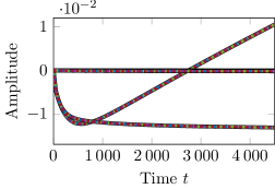
(a) Time response.

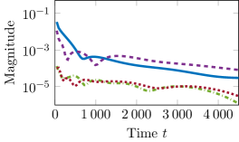
(b) Relative errors.

Figure 1: Time domain simulation results for the steel profile.

We first consider a classical, unstructured bilinear system as in Eq. 2. For the optimal cooling of steel profiles, the heat transfer process is described by the two dimensional heat equation

$$c\rho\partial_{t}v(t,\zeta)-\lambda\Delta v(t,\zeta) =0,$$

$$v(0,\zeta) =v_{0}(\zeta),$$

with $(t,\zeta)\in(0,t_{\mathrm{f}})\times\Omega$, the initial value $v_{0}(\zeta)\in\Omega$, and the Robin boundary conditions

$$\lambda\partial_{\nu}v(t,\zeta) =\left\{\begin{aligned} q_{i}u_{i}(t)\big{(}1-v(t,\zeta)\big{)},&&&\text{on}\leavevmode\nobreak\ \Gamma_{i},i=1,\ldots,6,\\ q_{7}\big{(}u_{7}(t)-v(t,\zeta)\big{)},&&&\text{on}\leavevmode\nobreak\ \Gamma_{7},\end{aligned}\right.$$

such that $\bigcup_{i=1}^{7}\Gamma_{i}=\partial\Omega$ and $\Gamma_{i}\cap\Gamma_{j}=\emptyset$ for $i\neq j$, where $\partial_{\nu}$ denotes the derivative in direction of the outer normal $\nu$ and $u_{i}(t)$ are the exterior cooling fluid temperatures used as controls. The spatial discretization of the rail shaped domain and parameters are chosen as described in [21, 25]. As a result, we consider a system of structure Eq. 2 with $n=5\,054\,209$ states, $m=7$ inputs, non-zero bilinear terms corresponding to the first $6$ inputs, and $p=6$ outputs. The data for this example is available in [26].

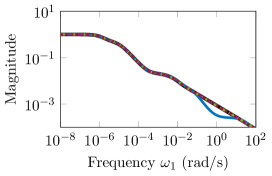
(a) Frequency response.

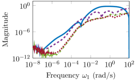
(b) Relative errors.

Figure 2: Frequency domain results of the first transfer functions for the steel profile.

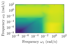
(a) $\mathsf{MtxInt}$.

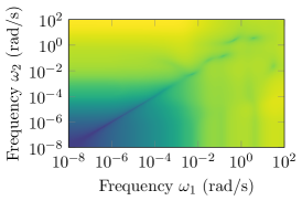
(b) $\mathsf{BwtInt}$.

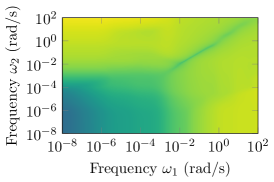
(c) $\mathsf{SftInt}$.

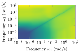
(d) $\mathsf{SttInt}$.

Figure 3: Frequency domain results of the second transfer functions for the steel profile.

The reduced-order models are constructed as follows:

MtxInt

with the interpolation points $\pm\texttt{logspace(-8, 2, 3)}\mathfrak{i}$ for the first and second subsystem transfer functions. Due to the rank deficiency in the generated columns, a rank truncation is performed to compress the model reduction basis, which yields a reduced-order model size of $r_{\mathsf{mtx}}=146$.

BwtInt

with the interpolation points $\pm\texttt{logspace(-8, 2, 8)}\mathfrak{i}$ for the first and second subsystem transfer functions resulting in the reduced order $r_{\mathsf{bwt}}=112$.

SftInt

with the interpolation points $\pm\texttt{logspace(-8, 2, 28)}\mathfrak{i}$ and the scaling vectors $d^{(i)}=\mathds{1}_{m}$ for the first and second subsystem transfer functions resulting in the reduced order $r_{\mathsf{sft}}=112$.

SttInt

with the interpolation points $\pm\texttt{logspace(-8, 2, 28)}\mathfrak{i}$ and the scaling vectors $d^{(i)}=b^{(i)}$ for the first and second subsystem transfer functions such that the reduced-order model size is $r_{\mathsf{stt}}=112$.

For all reduced-order models, we have chosen the same interval for the interpolation points. However, since the reduced-order dimension grows differently for different approaches, the number of interpolation points over the same interval differs so that the reduced-order models have the same (or at least comparable) order. For all directions, normalized random vectors from a uniform distribution on $[0,1]$ have been used. For all reduced-order models only one-sided projections ($W$ is set to $W=V$) have been applied resulting in reduced-order models having asymptotically stable linear parts. Note that the matrix interpolation has a much larger reduced order as anticipated.

Figure 1 shows the results for a time simulation using a unit step signal as input. All reduced-order models yield accurate approximations. The relative errors reveal that overall, $\mathsf{SftInt}$ and $\mathsf{SttInt}$ perform best, while $\mathsf{MtxInt}$ and $\mathsf{BwtInt}$ are several orders of magnitude worse in accuracy over the whole time interval. The maximum errors attained are given in Table 1. There, the two new tangential approaches $\mathsf{SftInt}$ and $\mathsf{SttInt}$ are both three orders of magnitude better than $\mathsf{MtxInt}$ for the time domain simulation.

The frequency domain analysis (Figures 2 and 3) illustrates similar conclusions. In the case of the first subsystem transfer function, $\mathsf{MtxInt}$ performs overall worst followed by $\mathsf{BwtInt}$. The new approaches $\mathsf{SftInt}$ and $\mathsf{SttInt}$ again show the smallest errors over the full frequency range. For the second transfer function level, all approaches behave comparable. The tangential approaches provide better errors than $\mathsf{MtxInt}$ if both frequency arguments are close to each other and $\mathsf{MtxInt}$ is more accurate for very small frequencies. For both transfer function levels, the maximum errors are given in Table 1.

Table 1: Maximum relative errors for the steel profile.

	$\boldsymbol{\mathsf{MtxInt}}$	$\boldsymbol{\mathsf{BwtInt}}$	$\boldsymbol{\mathsf{SftInt}}$	$\boldsymbol{\mathsf{SttInt}}$
$\operatorname{err}_{\mathrm{sim}}$	$4.0019\texttt{e-}01$	$1.6248\texttt{e-}02$	$3.2016\texttt{e-}04$	$3.3950\texttt{e-}04$
$\operatorname{err}_{\mathrm{G_{1}}}$	$6.3977\texttt{e-}01$	$2.0925\texttt{e-}01$	$2.3971\texttt{e-}02$	$1.9581\texttt{e-}02$
$\operatorname{err}_{\mathrm{G_{2}}}$	$2.1258\texttt{e+}00$	$5.0533\texttt{e+}00$	$3.1073\texttt{e+}00$	$2.6049\texttt{e+}00$

4.2 Time-delayed heated rod

Here, we consider the single-input/single-output structured bilinear system from [16, 10] that models a heated rod with distributed control and homogeneous Dirichlet boundary conditions, which is cooled by a delayed feedback. The underlying dynamics are described by the one dimensional heat equation

$$\partial_{t}v(t,\zeta) =\Delta v(t,\zeta)-2\sin(\zeta)v(t,\zeta)+2\sin(\zeta)v(t-1,\zeta)+u(t),$$ (42)

with $(t,\zeta)\in(0,t_{\mathrm{f}})\times(0,\pi)$ and boundary conditions $v(t,0)=v(t,\pi)=0$ for all $t\in[0,t_{\mathrm{f}}]$. As extension of Eq. 42 to the MIMO case, we consider independent control signals on equally sized sections of the rod as well as analogous measurements. Using centered differences for the spatial discretization, we obtain the bilinear time-delay system

$$\dot{x}(t) =Ax(t)+A_{\mathrm{d}}x(t-1)+\sum\limits_{k=1}^{m}N_{k}x(t)u_{k}(t)+Bu(t),$$

$$y(t) =Cx(t),$$

with $A,A_{\mathrm{d}},N_{k}\in\mathbb{R}^{n\times n}$, for $k=1,\ldots,m$, $B\in\mathbb{R}^{n\times m}$ and $C\in\mathbb{R}^{p\times n}$. For our experiments, we have chosen $n=5\,000$, $m=5$ and $p=2$.

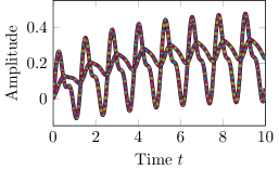
(a) Time response.

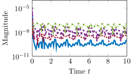
(b) Relative errors.

Figure 4: Time domain simulation results for the time-delayed heated rod.

The reduced-order models are constructed as follows:

MtxInt

with the interpolation points $\pm 1\mathfrak{i}$ for the first and second subsystem transfer functions. To overcome stability issues, only a one-sided projection was applied. The generated columns for the basis are rank deficient, therefore, a rank truncation has been performed to compress the model reduction basis resulting in the reduced order $r_{\mathsf{mtx}}=36$.

BwtInt

with the interpolation points $\pm\texttt{logspace(-4, 4, 3)}\mathfrak{i}$ for the first and second subsystem transfer functions with two-sided projection yielding the reduced order $r_{\mathsf{bwt}}=36$.

SftInt

with the interpolation points $\pm\texttt{logspace(-4, 4, 9)}\mathfrak{i}$ and the scaling vectors $d^{(i)}=\mathds{1}_{m}$ for the first and second subsystem transfer functions with two-sided projection to get a reduced-order model of size $r_{\mathsf{sft}}=36$.

SttInt

with the interpolation points $\pm\texttt{logspace(-4, 4, 9)}\mathfrak{i}$ and the scaling vectors $d^{(i)}=b^{(i)}$ for the first and second subsystem transfer functions with two-sided projection to get a reduced-order model of size $r_{\mathsf{stt}}=36$.

For all directions, normalized random vectors from a uniform distribution on $[0,1]$ have been used. Note that all reduced-order models have the same time-delay structure as the original system Eq. 42. All reduced-order models are chosen to be of the same size.

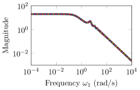
(a) Frequency response.

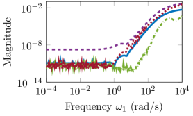
(b) Relative errors.

Figure 5: Frequency domain results of the first transfer functions for the time-delayed heated rod.

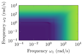
(a) $\mathsf{MtxInt}$.

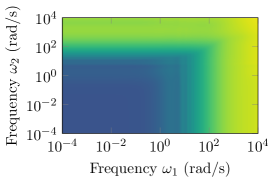
(b) $\mathsf{BwtInt}$.

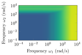
(c) $\mathsf{SftInt}$.

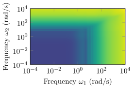
(d) $\mathsf{SttInt}$.

Figure 6: Frequency domain results of the second transfer functions for the time-delayed heated rod.

Figure 4 shows the results in time domain for the input signal

$$u(t) =\begin{bmatrix}0.05(\cos(10t)+\cos(5t))&0.05(\sin(10t)+\sin(5t))&0.01&0.01&0.01\end{bmatrix}^{\mkern-1.5mu\mathsf{T}}.$$

This time, $\mathsf{MtxInt}$ is a few orders of magnitude better than the other methods in the overall behavior closely followed by $\mathsf{SttInt}$, then $\mathsf{BwtInt}$ and $\mathsf{SftInt}$. But in terms of the maximum errors (Table 2), $\mathsf{SftInt}$ and $\mathsf{SttInt}$ are almost one order of magnitude better than $\mathsf{MtxInt}$. The results are different in frequency domain. Figure 5 shows the results for the first subsystem transfer functions. While $\mathsf{BwtInt}$ still performs worst, $\mathsf{SftInt}$ performs now better than $\mathsf{MtxInt}$, which is also shown in Table 2. The error of $\mathsf{SttInt}$ is mainly following $\mathsf{MtxInt}$ over the whole frequency range and only minorly diverging at the end. This changes for the second transfer functions in Figure 6. Here, $\mathsf{MtxInt}$ performs best with $\mathsf{SttInt}$ having comparable accuracy. $\mathsf{BwtInt}$ and $\mathsf{SftInt}$ are worse than the other two approaches but both with a comparable error. In terms of the maximum errors (Table 2), $\mathsf{BwtInt}$ and $\mathsf{MtxInt}$ perform the best.

Further results for tangential interpolation of a related example using different choices of interpolation points can be found in [28, Sec. 5.6.5.2].

Table 2: Maximum relative errors for the time-delayed heated rod.

	$\boldsymbol{\mathsf{MtxInt}}$	$\boldsymbol{\mathsf{BwtInt}}$	$\boldsymbol{\mathsf{SftInt}}$	$\boldsymbol{\mathsf{SttInt}}$
$\operatorname{err}_{\mathrm{sim}}$	$1.2251\texttt{e-}06$	$1.2111\texttt{e-}05$	$2.1393\texttt{e-}07$	$5.2099\texttt{e-}07$
$\operatorname{err}_{\mathrm{G_{1}}}$	$5.0048\texttt{e-}03$	$4.2078\texttt{e-}02$	$5.1565\texttt{e-}04$	$3.6159\texttt{e-}02$
$\operatorname{err}_{\mathrm{G_{2}}}$	$8.6292\texttt{e-}03$	$8.3005\texttt{e-}02$	$4.2940\texttt{e-}02$	$2.0130\texttt{e-}01$

4.3 Damped mass-spring system with bilinear springs

As the third and final example, we consider the MIMO bilinear damped mass-spring system from [10]. The system has a mechanical second-order structure as the example Eq. 1 and takes the form

$$\begin{aligned} M\ddot{x}(t)+D\dot{x}(t)+Kx(t)&=N_{\mathrm{p},1}x(t)u_{1}(t)+N_{\mathrm{p},2}x(t)u_{2}(t)+B_{\mathrm{u}}u(t),\\ y(t)&=C_{\mathrm{p}}x(t),\end{aligned}$$ (43)

where $M,D,K\in\mathbb{R}^{n\times n}$ are symmetric positive definite matrices chosen as in [18]. The external forces are applied to the first and last masses, $B_{\mathrm{u}}=[e_{1},-e_{n}]$, the displacement of the second and fifth masses is observed, $C_{\mathrm{p}}=[e_{2},e_{5}]^{\mkern-1.5mu\mathsf{T}}$; thus the system has $m=p=2$ inputs and outputs. The bilinear springs are chosen to be

$$\begin{aligned} N_{\mathrm{p},1}&=-S_{1}KS_{1}&\text{and}&&N_{\mathrm{p},2}&=S_{2}KS_{2},\end{aligned}$$

where $S_{1}$ is a diagonal matrix with entries linspace(0.2,0,n) and $S_{2}$ a diagonal matrix with linspace(0,0.2,n). For the experiments, we chose $n=1\,000$.

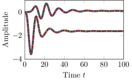
(a) Time response.

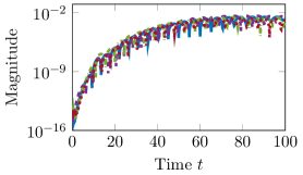
(b) Relative errors.

Figure 7: Time domain simulation results for the damped mass-spring system.

It has already been shown in [10] that only the structure-preserving approximations give reasonable results for this example. Therefore, we only compare the structured approaches in this paper, i.e., all reduced-order models also have the mechanical system structure as Eq. 43. The reduced-order models are constructed as follows:

MtxInt

with the interpolation points $\pm\texttt{logspace(-4, 4, 2)}\mathfrak{i}$ for the first and second subsystem transfer functions, which yields the reduced order $r_{\mathsf{mtx}}=24$.

BwtInt

with the interpolation points $\pm\texttt{logspace(-4, 4, 4)}\mathfrak{i}$ for the first and second subsystem transfer functions such that the reduced order is $r_{\mathsf{bwt}}=24$.

SftInt

with the interpolation points $\pm\texttt{logspace(-4, 4, 6)}\mathfrak{i}$ and the scaling vectors $d^{(i)}=\mathds{1}_{m}$ for the first and second subsystem transfer functions such that the reduced order is $r_{\mathsf{sft}}=24$.

SttInt

with interpolation points $\pm\texttt{logspace(-4, 4, 6)}\mathfrak{i}$ and the scaling vectors $d^{(i)}=b^{(i)}$ for the first and second subsystem transfer functions such that the reduced order is $r_{\mathsf{stt}}=24$.

To preserve the symmetry of the system matrices, only one-sided projections have been used for the construction. For all directions, normalized random vectors have been generated by drawing their entries from a uniform distribution on $[0,1]$. All reduced-order models have the same order.

Figure 7 shows the time simulation results for

$$u(t) =\begin{bmatrix}\sin(200t)+200\\ -\cos(200t)-200\end{bmatrix}.$$

All reduced-order models yield accurate results with practically the same approximation quality. As Table 3 shows, the new tangential approaches perform a little bit better than $\mathsf{MtxInt}$ but still have the same order of accuracy. Also, in the frequency domain, the tangential interpolation as well as the matrix interpolation behave in principle all the same, where the matrix interpolation is again a bit worse than the tangential approaches as it can be seen in Figures 8 and 9, and Table 3.

Further results for tangential interpolation of a related example using different choices of interpolation points can be found in [28, Sec. 5.6.5.1].

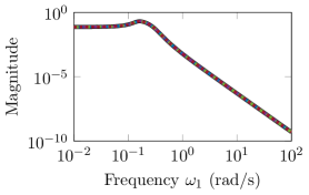
(a) Frequency response.

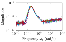
(b) Relative errors.

Figure 8: Frequency domain results of the first transfer functions for the damped mass-spring system.

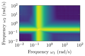
(a) $\mathsf{MtxInt}$.

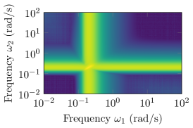
(b) $\mathsf{BwtInt}$.

(c) $\mathsf{SftInt}$.

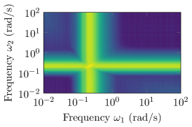
(d) $\mathsf{SttInt}$.

Figure 9: Frequency domain results of the second transfer functions for the damped mass-spring system.

Table 3: Maximum relative errors for the damped mass-spring system.

	$\boldsymbol{\mathsf{MtxInt}}$	$\boldsymbol{\mathsf{BwtInt}}$	$\boldsymbol{\mathsf{SftInt}}$	$\boldsymbol{\mathsf{SttInt}}$
$\operatorname{err}_{\mathrm{sim}}$	$3.0779\texttt{e-}03$	$4.0813\texttt{e-}03$	$2.8056\texttt{e-}03$	$1.9722\texttt{e-}03$
$\operatorname{err}_{\mathrm{G_{1}}}$	$6.3187\texttt{e-}05$	$5.0642\texttt{e-}05$	$5.7109\texttt{e-}05$	$3.2660\texttt{e-}05$
$\operatorname{err}_{\mathrm{G_{2}}}$	$4.5523\texttt{e-}04$	$4.3227\texttt{e-}04$	$4.2240\texttt{e-}04$	$2.8460\texttt{e-}04$

5 Conclusions

We developed the tangential interpolation framework for structure-preserving interpolation of multi-input/multi-output bilinear control systems. By revisiting the classical tangential interpolation in frequency domain and its interpretation in time domain, we developed a new unifying tangential interpolation framework for structure-preserving model reduction of MIMO bilinear systems and proved conditions on the model reduction subspaces to satisfy interpolation conditions in this new framework. We also used the new framework to obtain results on the blockwise tangential interpolation approach and extended the theory from the literature to structured bilinear systems. While the new framework was motivated by classical tangential interpolation in frequency domain and its interpretation in time domain, the generality of this new approach and the corresponding theorems is that not only the existing framework to tangential interpolation can be obtained as a special case of the new framework but also it offers even more flexibility and options in the model reduction procedure than explored in this paper. The numerical examples illustrate that the new approach is as good as and even better in many situation than the full matrix or the blockwise tangential interpolation methods. In other words, the new approach gives sufficiently accurate results while allowing more freedom in choosing the order of the reduced-order model compared to the existing approaches.

While we used a rather simple choice for interpolation points (logarithmically equidistant on the imaginary axis), the question of better or even optimal choices of interpolation points remains open. Other choices for interpolation point selections, heuristically inspired by the linear system case, have been used in numerical examples in [28]. Also, in the setting of tangential interpolation, the question of appropriate tangential directions needs to be answered. For our new framework, we gave two approaches for choosing the scaling vectors. Still the influence of the choice of the scaling vectors needs to be investigated as well as the question of an optimal choice. These issue will be considered in future works.

References

- [1] Al-Baiyat, S., Farag, A.S., Bettayeb, M.: Transient approximation of a bilinear two-area interconnected power system. Electr. Power Syst. Res. 26(1), 11–19 (1993). 10.1016/0378-7796(93)90064-L
- [2] Antoulas, A.C., Beattie, C.A., Gugercin, S.: Interpolatory Methods for Model Reduction. Computational Science & Engineering. SIAM, Philadelphia, PA (2020). 10.1137/1.9781611976083
- [3] Antoulas, A.C., Gosea, I.V., Ionita, A.C.: Model reduction of bilinear systems in the Loewner framework. SIAM J. Sci. Comput. 38(5), B889–B916 (2016). 10.1137/15M1041432
- [4] Bai, Z., Skoogh, D.: A projection method for model reduction of bilinear dynamical systems. Linear Algebra Appl. 415(2–3), 406–425 (2006). 10.1016/j.laa.2005.04.032
- [5] Ball, J.A., Gohberg, I., Rodman, L.: Interpolation of Rational Matrix Functions, Operator Theory: Advances and Applications, vol. 45. Birkhäuser, Basel (1990). 10.1007/978-3-0348-7709-1
- [6] Beattie, C.A., Gugercin, S.: Interpolatory projection methods for structure-preserving model reduction. Syst. Control Lett. 58(3), 225–232 (2009). 10.1016/j.sysconle.2008.10.016
- [7] Benner, P., Breiten, T.: Interpolation-based -model reduction of bilinear control systems. SIAM J. Matrix Anal. Appl. 33(3), 859–885 (2012). 10.1137/110836742
- [8] Benner, P., Breiten, T., Damm, T.: Generalized tangential interpolation for model reduction of discrete-time MIMO bilinear systems. Int. J. Control 84(8), 1398–1407 (2011). 10.1080/00207179.2011.601761
- [9] Benner, P., Damm, T.: Lyapunov equations, energy functionals, and model order reduction of bilinear and stochastic systems. SIAM J. Control Optim. 49(2), 686–711 (2011). 10.1137/09075041X
- [10] Benner, P., Gugercin, S., Werner, S.W.R.: Structure-preserving interpolation of bilinear control systems. Adv. Comput. Math. 47(3), 43 (2021). 10.1007/s10444-021-09863-w
- [11] Breiten, T., Damm, T.: Krylov subspace methods for model order reduction of bilinear control systems. Syst. Control Lett. 59(8), 443–450 (2010). 10.1016/j.sysconle.2010.06.003
- [12] Condon, M., Ivanov, R.: Krylov subspaces from bilinear representations of nonlinear systems. Compel-Int. J. Comp. Math. Electr. Electron. Eng. 26(2), 399–406 (2007). 10.1108/03321640710727755
- [13] Feng, L., Benner, P.: A note on projection techniques for model order reduction of bilinear systems. AIP Conf. Proc. 936(1), 208–211 (2007). 10.1063/1.2790110
- [14] Flagg, G.M., Gugercin, S.: Multipoint Volterra series interpolation and optimal model reduction of bilinear systems. SIAM J. Matrix Anal. Appl. 36(2), 549–579 (2015). 10.1137/130947830
- [15] Gallivan, K., Vandendorpe, A., Van Dooren, P.: Model reduction of MIMO systems via tangential interpolation. SIAM J. Matrix Anal. Appl. 26(2), 328–349 (2004). 10.1137/S0895479803423925
- [16] Gosea, I.V., Pontes Duff, I., Benner, P., Antoulas, A.C.: Model order reduction of bilinear time-delay systems. In: Proc. of 18th European Control Conference (ECC), pp. 2289–2294 (2019). 10.23919/ECC.2019.8796085
- [17] Hsu, C.S., Desai, U.B., Crawley, C.A.: Realization algorithms and approximation methods of bilinear systems. In: The 22nd IEEE Conference on Decision and Control, pp. 783–788 (1983). 10.1109/CDC.1983.269628
- [18] Mehrmann, V., Stykel, T.: Balanced truncation model reduction for large-scale systems in descriptor form. In: P. Benner, V. Mehrmann, D.C. Sorensen (eds.) Dimension Reduction of Large-Scale Systems, Lect. Notes Comput. Sci. Eng., vol. 45, pp. 83–115. Springer, Berlin, Heidelberg (2005). 10.1007/3-540-27909-1_3
- [19] Mohler, R.R.: Natural bilinear control processes. IEEE Transactions on Systems Science and Cybernetics 6(3), 192–197 (1970). 10.1109/TSSC.1970.300341
- [20] Mohler, R.R.: Bilinear Control Processes: With Applications to Engineering, Ecology and Medicine, Mathematics in Science and Engineering, vol. 106. Academic Press, New York, London (1973)
- [21] Oberwolfach Benchmark Collection: Steel profile. Hosted at MORwiki – Model Order Reduction Wiki (2005). URL http://modelreduction.org/index.php/Steel_Profile
- [22] Qian, K., Zhang, Y.: Bilinear model predictive control of plasma keyhole pipe welding process. J. Manuf. Sci. Eng. 136(3), 031002 (2014). 10.1115/1.4025337
- [23] Rodriguez, A.C., Gugercin, S., Boggaard, J.: Interpolatory model reduction of parameterized bilinear dynamical systems. Adv. Comput. Math. 44(6), 1887–1916 (2018). 10.1007/s10444-018-9611-y
- [24] Rugh, W.J.: Nonlinear System Theory: The Volterra/Wiener Approach. The Johns Hopkins University Press, Baltimore (1981)
- [25] Saak, J.: Effiziente numerische Lösung eines Optimalsteuerungsproblems für die Abkühlung von Stahlprofilen. Diploma thesis, Universität Bremen, Germany (2003). 10.5281/zenodo.1187041
- [26] Saak, J., Köhler, M., Benner, P.: M-M.E.S.S. – The Matrix Equations Sparse Solvers library (version 2.1) (2021). 10.5281/zenodo.4719688. See also: https://www.mpi-magdeburg.mpg.de/projects/mess
- [27] Saputra, J., Saragih, R., Handayani, D.: Robust controller for bilinear system to minimize HIV concentration in blood plasma. J. Phys.: Conf. Ser. 1245, 012055 (2019). 10.1088/1742-6596/1245/1/012055
- [28] Werner, S.W.R.: Structure-preserving model reduction for mechanical systems. Dissertation, Otto-von-Guericke-Universität, Magdeburg, Germany (2021). 10.25673/38617
- [29] Werner, S.W.R.: Code, data and results for numerical experiments in “A unifying framework for tangential interpolation of structured bilinear control systems” (version 1.0) (2022). 10.5281/zenodo.5793356
- [30] Zhang, L., Lam, J.: On model reduction of bilinear systems. Automatica J. IFAC 38(2), 205–216 (2002). 10.1016/S0005-1098(01)00204-7