Efficient Solution of Discrete Subproblems Arising in Integer Optimal Control with Total Variation Regularization

Abstract

We consider a class of integer linear programs (IPs) that arise as discretizations of trust-region subproblems of a trust-region algorithm for the solution of control problems, where the control input is an integer-valued function on a one-dimensional domain and is regularized with a total variation term in the objective, which may be interpreted as a penalization of switching costs between different control modes.

We prove that solving an instance of the considered problem class is equivalent to solving a resource constrained shortest path problem (RCSPP) on a layered directed acyclic graph. This structural finding yields an algorithmic solution approach based on topological sorting and corresponding run time complexities that are quadratic in the number of discretization intervals of the underlying control problem, the main quantifier for the size of a problem instance. We also consider the solution of the RCSPP with an $A^{*}$ algorithm. Specifically, the analysis of a Lagrangian relaxation yields a consistent heuristic function for the $A^{*}$ algorithm and a preprocessing procedure, which can be employed to accelerate the $A^{*}$ algorithm for the RCSPP without losing optimality of the computed solution.

We generate IP instances by executing the trust-region algorithm on several integer optimal control problems. The numerical results show that the accelerated $A^{*}$ algorithm and topological sorting outperform a general purpose IP solver significantly. Moreover, the accelerated $A^{*}$ algorithm is able to outperform topological sorting for larger problem instances.

1 Introduction

Integer optimal control problems (IOCPs)—optimization problems constrained by (partial) differential equations with integer-valued control input functions—are versatile modeling tools with diverse applications from topology optimization, see e.g. Svanberg and Werme, (2007), Haslinger and Mäkinen, (2015), Liang and Cheng, (2019), Leyffer et al., (2021), over energy management of buildings, see e.g. Zavala et al., (2010), to network transportation problems, e.g. traffic flow as considered in Göttlich et al., (2014, 2017) or gas flow as considered in Pfetsch et al., (2015), Hante et al., (2017), Habeck et al., (2019).

A computationally efficient algorithmic solution approach that provides optimal approximation properties for many IOCPs under appropriate assumptions on the underlying differential equations is the so-called combinatorial integral approximation, see e.g. Sager et al., (2011, 2012), Hante and Sager, (2013), Jung et al., (2015), Manns and Kirches, (2020), Kirches et al., (2021).

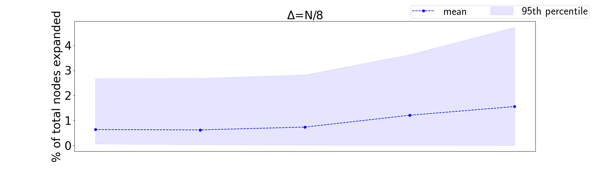
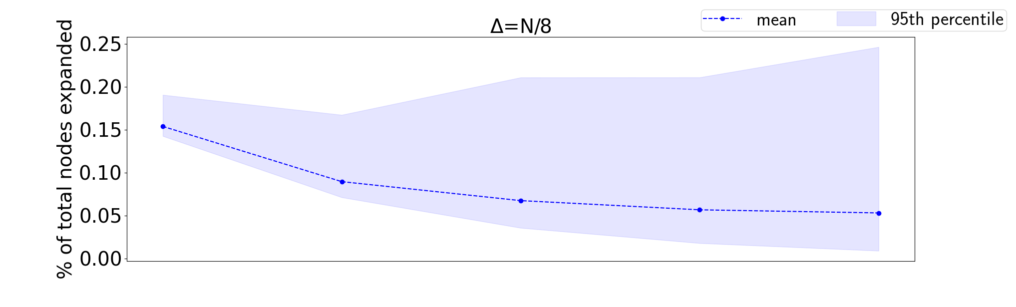
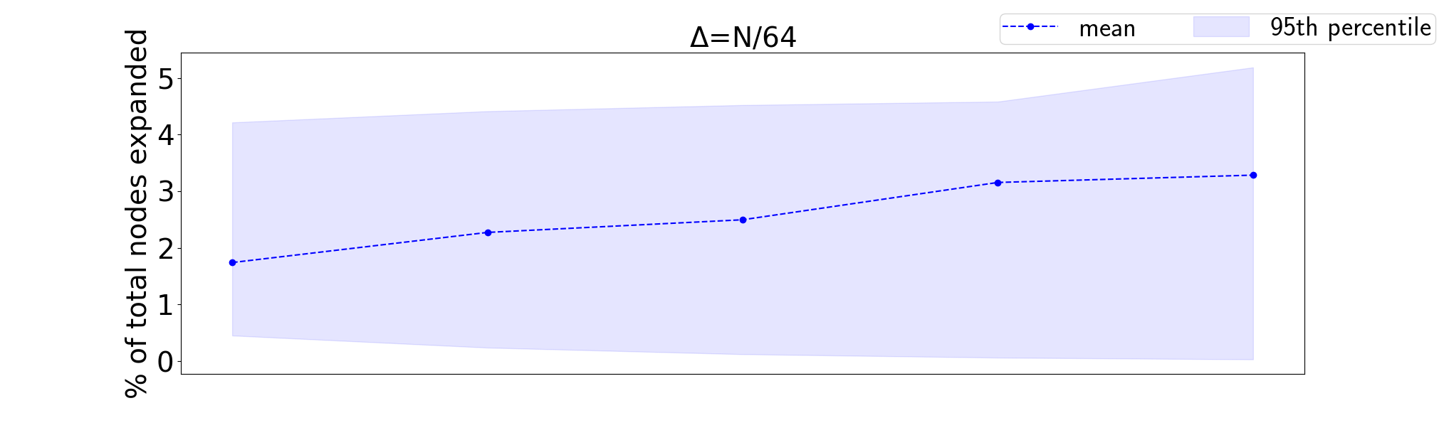
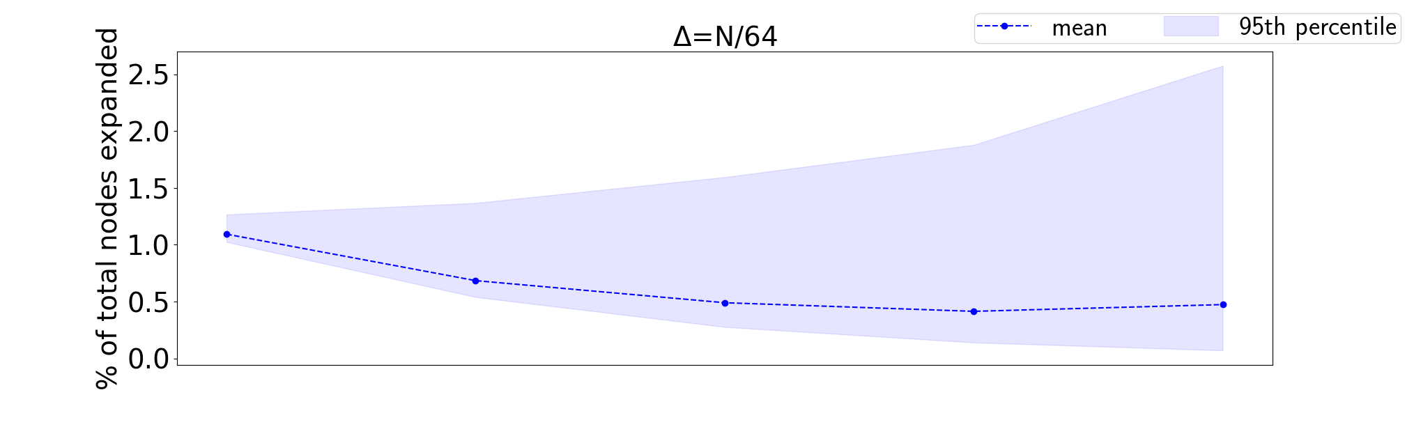
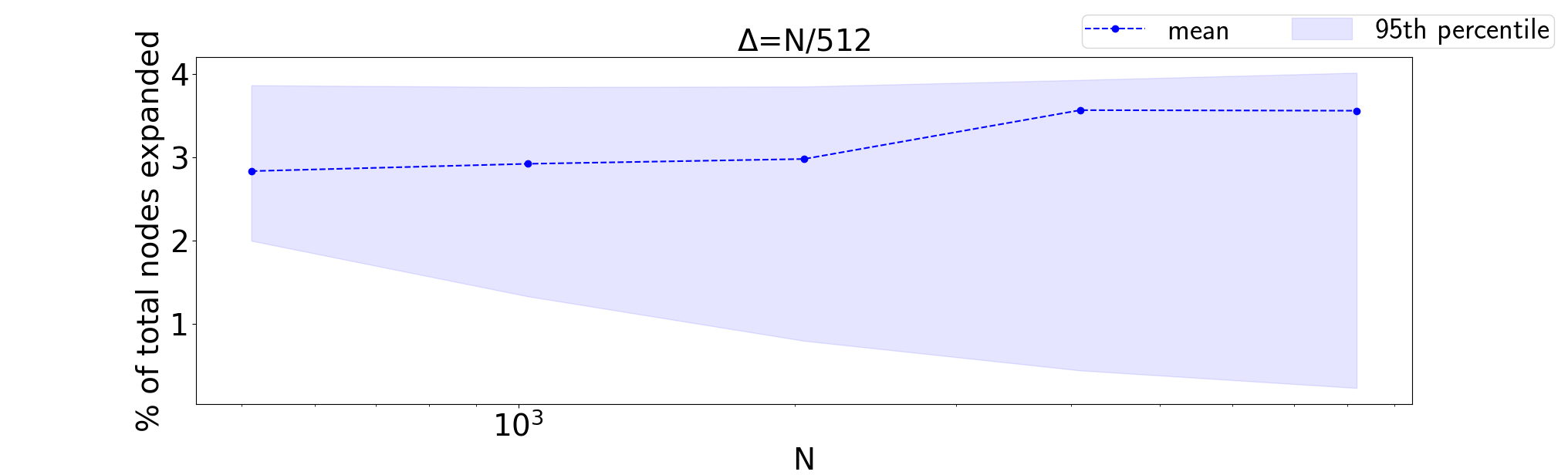
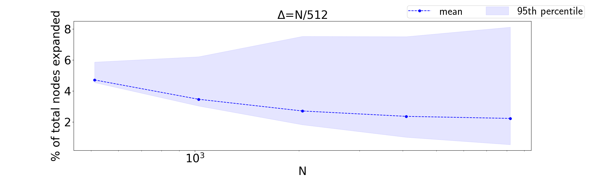
Figure 5: Mean percentage of nodes (blue, dashed) expanded by LABEL:itm:astar for different values of $N$ for the graphs of the (TR-IP) instances stemming from (SH) (left) and (SR) (right). The lightly colored areas represent the 95th percentile of expanded nodes, that is 5 percent of the instances expand a larger fraction of the nodes in the graph. The trust-region radii $\Delta$ are $\frac{1}{8}N$ (top), $\frac{1}{64}N$ (center) and $\frac{1}{512}N$ (bottom).

The optimality principle underlying the combinatorial integral approximation comes at the cost of high-frequency switching of the resulting control input function between different integers, see Figure 5 in Manns and Kirches, (2020) or Figures 3 and 4 Kirches et al., (2021), which impairs the implementability of the resulting controls. This behavior cannot be avoided if an optimal control function for the continuous relaxation is not already integer-valued. Recent research has produced results to alleviate this problem by promoting integer-valued control functions in the continuous relaxation, see Manns, (2021), and minimizing switching costs while maintaining approximation guarantees in the combinatorial integral approximation, see Bestehorn et al., (2019, 2020), Bestehorn and Kirches, (2020), Bestehorn et al., (2021), Sager and Zeile, (2021).

However, even combining both approaches cannot avoid this problem in many situations as is pointed out and visualized in sections 4 and 5 in Manns, (2021), which motivates to seek alternative approaches to mitigate high-frequency oscillations in IOCPs. Leyffer and Manns, (2021) propose a novel trust-region algorithm, which—after discretization of the underlying differential equation—produces a sequence of integer linear programs (IPs) as trust-region subproblems for control functions that are defined on one-dimensional domains. Switching costs are modeled with a penalty in the objective and not approximated but modeled exactly with linear inequalities in each subproblem, thereby yielding a structure-preserving algorithm. The subproblems are solved with a general purpose IP solver in Leyffer and Manns, (2021), which yields run times that are several orders of magnitude higher than those of the combinatorial integral approximation, specifically the approach proposed in Bestehorn et al., (2020), where switching costs in the form of penalty terms are considered in the approximation problems. This shortcoming is addressed in this work.

Contribution

Minimizing switching costs in the combinatorial integral approximation with penalty terms are treated with a shortest path approach in Bestehorn et al., (2020). We transfer these ideas to the trust-region subproblems that arise in algorithm proposed in Leyffer and Manns, (2021) and prove equivalence to resource constrained shortest path problems (RCSPPs) on layered directed acyclic graphs (LDAGs).

We provide run time estimates of a topological sorting approach and analyze an $A^{*}$ algorithm for the resulting RCSPPs, which yields that both approaches are pseudo-polynomial solution algorithms and the problem is fixed-parameter tractable. In particular, we show that the subproblems are generally NP-hard but the NP-hardness stems from the set of integers that constitute the admissible values for the control function of the underlying IOCP. This set is constant over all subproblems of one run of the trust-region algorithm and generally small, usually containing only between 2 and 10 values depending on the application.

We analyze a Lagrangian relaxation of the IP formulation that yields upper and lower bounds on subpaths in the RCSPP formulation and provides a consistent and monotone heuristic, which yields that an $A^{*}$ algorithm can be accelerated without losing optimality of the computed path. We also analyze a dominance principle to further reduce the search space. We evaluate the approach by executing the trust-region algorithm on instances of two classes of IOCPs. We solve the generated subproblems with different algorithmic approaches, specifically topological sorting, the general purpose IP solver SCIP, see Gamrath et al., (2020), and the $A^{*}$ algorithm with the aforementioned accelerations. The general purpose IP solver is several orders of magnitude slower than the other two approaches. The $A^{*}$ algorithm is able to outperform topological sorting for larger sizes of the subproblems, thereby suggesting to choose the subproblem solver depending on the subproblem size.

Structure of the Remainder

We introduce some notation that we use in the remainder of the manuscript below. Then we introduce the superordinate IOCPs and the trust-region algorithm in §2. We continue by presenting and analyzing the IPs that arise as discretized trust-region subproblems and which are the main object of our investigation in §3, where we also show their equivalence to RCSPPs on LDAGs. We show how the $A^{*}$ algorithm may be accelerated using information obtained from the Lagrangian Relaxation in §4. The set of our computational experiments is described §5. The results are presented in §6. We draw a conclusion in §7.

Notation

For a natural number $n\in\mathbb{N}$ we define the notation $[n]\coloneqq\{1,\ldots,n\}$. For a scalar $a\in\mathbb{R}$ and a set $B\subset\mathbb{R}$ we abbreviate $B-a\coloneqq\{b-a\,|\,b\in B\}$.

2 IOCPs and Trust-region Algorithm

We briefly state the trust-region algorithm and the class of IOCPs such that the analyzed problems arise as trust-region subproblems after discretization. The general IOCP reads

$$\begin{aligned} \min_{x\in L^{2}(0,T)}&F(x)+\alpha\operatorname*{TV}(x)\eqqcolon J(x)\\ \text{~{}~{}s.t.~{}~{}}&x(t)\in\Xi\text{ for almost all (a.a.) }t\in(0,T),\end{aligned}$$ (IOCP)

where $T>0$, $L^{1}(0,T)$ and $L^{2}(0,T)$ denote the spaces of integrable and square-integrable functions on $(0,T)$, $F:L^{2}(0,T)\to\mathbb{R}$ denotes the main part of the objective that abstracts from the underlying differential equation, $x$ is the optimized $\Xi$-valued control function, and $\Xi\subset\mathbb{Z}$ is a finite set of integers. The term $\alpha\operatorname*{TV}(x)$ models the switching costs of the function $x$, where $\alpha>0$ is a positive scalar and $\operatorname*{TV}(x)\in[0,\infty]$ is the total variation of $x$, which amounts to the sum of the jump heights of $x$ because $x$ takes only finitely many values, see Leyffer and Manns, (2021).

The trust-region subproblem that is proposed in Leyffer and Manns, (2021) reads

$$\begin{aligned} \min_{d\in L^{1}(0,T)}&(\nabla F(x),d)_{L^{2}(0,T)}+\alpha\operatorname*{TV}(x+d)-\alpha\operatorname*{TV}(x)\eqqcolon\ell(x,d)\\ \text{~{}~{}s.t.~{}~{}}&x(t)+d(t)\in\Xi\text{ for a.a.\ }t\in(0,T),\\ &\|d\|_{L^{1}(0,T)}\leq\Delta\end{aligned}$$ (TR)

for a trust-region radius $\Delta>0$. We denote the instance of (TR) for a given control function $x$ and a given trust-region radius $\Delta>0$ by $\operatorname*{TR}(x,\Delta)$.

The trust-region algorithm is given in Algorithm 1 and works as follows. In every outer iteration (indexed by $n$) the trust-region radius is reset to the input $\Delta^{0}>0$ and an inner loop (iteration index $k$) is triggered. In the inner iteration the trust-region subproblem is solved for the trust-region radius. Then the algorithm terminates if the predicted reduction (objective of the trust-region subproblem) is zero for a positive trust-region radius, which implies a necessary optimality condition under appropriate assumptions on the function $F$ according to Leyffer and Manns, (2021). If the computed iterate can be accepted—that is, if the actual reduction is at least a fraction of the linearly predicted reduction—the inner loop terminates and the current iterate is updated. If the step cannot be accepted (is rejected), then the trust-region is halved and the next inner iteration of the inner loop is triggered.

Algorithm 1 Sketch of the trust-region algorithm from Leyffer and Manns, (2021)

Input: $x^{0}$ feasible for (IOCP), $\Delta^{0}>0$, $\rho\in(0,1)$

1:for $n=1,\ldots$ do

2:     $k\leftarrow 0$, $\Delta^{n,0}\leftarrow\Delta^{0}$

3:     repeat

4:         $d^{n,k}\leftarrow$ minimizer of $\operatorname*{TR}(x^{n-1},\Delta^{n,k})$ $\triangleright$ Compute step.

5:         if $\ell(x^{n-1},d)=0$ then $\triangleright$ The predicted reduction is zero.

6:              Terminate with solution $x^{n-1}$.

7:         else if $J(x^{n-1})-J(x^{n-1}+d^{n,k})<\rho\ell(x^{n-1},d^{n,k})$ then $\triangleright$ Reject step.

8:              $\Delta^{n,k+1}\leftarrow\Delta^{n,k}/2$, $k\leftarrow k+1$

9:         else$\triangleright$ Accept step.

10:              $x^{n}\leftarrow x^{n-1}+d^{n,k}$, $k\leftarrow k+1$

11:         end if

12:     until $J(x^{n-1})-J(x^{n-1}+d^{n,k})\geq\sigma\ell(x^{n-1},d^{n,k})$

13:end for

3 The Discretized Trust-region Subproblem

We provide and explain the IP formulation of the considered problem class in §3.1 for which we show the NP-hardness in §3.2. Then we construct an LDAG and prove that a shortest path search on it is equivalent to solving the IP formulation in §3.3. In §3.4 we factorize the graph by means of an equivalence relation and obtain the aforementioned equivalence to an RCSPP on the resulting reduced graph (quotient graph). In §3.5 we present two algorithms to solve the SPP on the LDAG, which are accelerated in §4 and compared computationally to a general purpose IP solver in §5.

3.1 IP Formulation

The optimization problem of our interest reads

$$\begin{aligned} \min_{d}\quad&\sum_{i=1}^{N}c_{i}d_{i}+\alpha\sum_{i=1}^{N-1}|x_{i+1}+d_{i+1}-x_{i}-d_{i}|\eqqcolon C(d)\\ \text{s.t.}\quad&x_{i}+d_{i}\in\Xi\text{ for all }i\in[N],\\ &\sum_{i=1}^{N}\gamma_{i}|d_{i}|\leq\Delta,\end{aligned}$$ (TR-IP)

where we have dropped a constant term from the objective. It arises from (TR) by discretizing of $(0,T)$ into $N\in\mathbb{N}$ intervals, see Leyffer and Manns, (2021). The absolute values can be replaced with linear inequality constraints by introducing auxiliary variables, which yields an IP formulation. Again, $\Xi=\{\xi_{1},\ldots,\xi_{m}\}\subset\mathbb{Z}$, with $\xi_{1}<\ldots<\xi_{m}$, $m\in\mathbb{N}$, denotes a finite set of integers. Because the control functions are $\Xi$-valued, we use the ansatz of interval-wise constant functions that are represented by the vector of step heights $x\in\Xi^{N}$. The latter is an input of (TR-IP) and contains the step heights of the previously accepted control function iterate in Algorithm 1. The vector $\gamma\in\mathbb{N}^{N}$ contains the lengths of the discretization intervals. For uniform discretization grids this means that $\gamma_{i}=1$ for all $i\in[N]$.

The variable $d\in(\Xi-x_{1})\times\ldots\times(\Xi-x_{N})$ denotes the optimal step given by the solution of (TR-IP), yielding the new discretized control function representative $x+d\in\Xi^{N}$. The term $\alpha\sum_{i=1}^{N-1}|x_{i+1}+d_{i+1}-x_{i}-d_{i}|$ in the objective models the sum of the jump heights between the subsequent intervals scaled by a penalty parameter $\alpha>0$, which is also an input of (TR-IP).

Finally, the vector $c\in\mathbb{R}^{N}$ is a further input of (TR-IP) and arises from a numerical approximation of $\nabla F(x)$ in (TR). We will frequently use this setting for the quantities in (TR-IP) and thus summarize it in the assumption below.

Assumption 1.

Let $c\in\mathbb{R}^{N}$, $\alpha\in\mathbb{R}_{\geq 0}$, $\Delta\in\mathbb{N}$, $\Xi=\{\xi_{1},\ldots,\xi_{m}\}\subset\mathbb{Z}$ with $\xi_{1}<\ldots<\xi_{m}$ for some $m\in\mathbb{N}$, $x\in\Xi^{N}$, and $\gamma\in\mathbb{N}^{N}$ be given.

Remark 2.

Our restriction to $\gamma_{i}\in\mathbb{N}$ means that the different mesh sizes have to be integer multiples of the smallest mesh size. While this does restrict the possible discretization grids severely, it enables our algorithmic approach with shortest path algorithms below, which does not generalize to arbitrary choices $\gamma_{i}\in(0,\infty)$.

Remark 3.

The inputs $x\in V^{N}$, $c\in\mathbb{R}^{N}$, and $\gamma\in\mathbb{N}^{N}$ may change in every outer iteration of Algorithm 1 (the latter only in the presence of an adaptive grid refinement and coarsening strategy) but are constant over the inner iterations of an outer iteration. The trust-region radius $\Delta>0$ changes in every inner iteration.

Remark 4.

We restrict the input $\Delta\in\mathbb{N}$ in our analysis to

$$\Delta\leq\Delta_{\max}\coloneqq(\max\Xi-\min\Xi)\|h\|_{\infty}N$$ (1)

because the constraint $\sum_{i=1}^{N}\gamma_{i}|d_{i}|\leq\Delta$ may be dropped in (TR-IP) if $\Delta\geq\Delta_{\max}$.

3.2 NP-hardness of (TR-IP)

The problem (TR-IP) resembles the Knapsack problem closely. If we set $\alpha=0$, $x=(0,\ldots,0)$ and $\Xi=\{0,1\}$, the problem is reduced to

$$\begin{aligned} \min_{d}\quad&\sum_{i=1}^{N}c_{i}d_{i}\\ \text{s.t.}\quad&d_{i}\in\{0,1\}\text{ for all }i\in[N]\text{ and }\sum_{i=1}^{N}\gamma_{i}|d_{i}|\leq\Delta,\end{aligned}$$

which is the well-known Knapsack problem. Obviously, the more general problem (TR-IP) is also NP-hard. We briefly show that even in the case of a uniform discretization grid, meaning $\gamma_{i}=1$ for all $i\in[N]$, (TR-IP) remains NP-hard.

Proposition 5.

Let Assumption 1 hold. The problem (TR-IP) with $\gamma_{i}=1$ for all $i\in[N]$ is NP-hard.

Proof.

Proof. We show the NP-hardness by a reduction from the Knapsack problem. Let $\tilde{c}_{1}$, $\ldots$, $\tilde{c}_{n}$ be the positive costs and $\tilde{w}_{1}$, $\ldots$, $\tilde{w}_{n}$ the positive integer weights of the $n$ items. Let $K$ be the budget of the Knapsack.

We set $\Delta=K$ and $N=2n+1$. Let $\alpha>0$ be an arbitrary but fixed. We construct $\Xi$ such that it contains $N+1$ elements of the form

$$\sum_{i=1}^{k}\tilde{w}_{i}+(k+1)(\Delta+1)\in\Xi\text{ for all }k\in\{0,\ldots,n-1\}$$

and $$\sum_{i=1}^{k}\tilde{w}_{i}+k(\Delta+1)\in\Xi\text{ for all }k\in\{0,\ldots,n\}.$$

In the case that $\Xi$ is ordered from smallest to largest, the difference between two subsequent elements is either $\Delta+1$ or the weight of an item. For all $i\in[N]$ we choose

$$x_{i}=\begin{cases}\sum_{j=1}^{\frac{i}{2}-1}\tilde{w}_{j}+\frac{i}{2}(\Delta+1)&\text{$i$ even},\\ 0&\text{$i$ odd}.\end{cases}$$

For odd $i$ this directly implies $d_{i}=0$, while for even $i$ it follows that $d_{i}=0$ or $d_{i}=\tilde{w}_{\frac{i}{2}}$. Furthermore, we set

$$c_{i}=\begin{cases}-\frac{\tilde{c}_{\frac{i}{2}}}{\tilde{w}_{\frac{i}{2}}}-2\alpha&\text{$i$ even},\\ 0&\text{$i$ odd}.\end{cases}$$

This leads to the reduced problem

$$\begin{aligned} \min_{d}\ &\sum_{i=1}^{n}c_{2i}d_{2i}+2\alpha\sum_{i=1}^{n}(x_{2i}+d_{2i})\\ \text{s.t.}\ &x_{i}+d_{i}\in V\text{ for all }i\in\{1,\ldots,N\}\\ &\sum_{i=1}^{n}|d_{2i}|\leq\Delta.\\ \end{aligned}$$

It follows from the choice of the $c_{i}$ that $c_{2i}d_{2i}+2\alpha d_{2i}=(-\frac{\tilde{c}_{i}}{\tilde{w}_{i}}-2\alpha)d_{2i}+2\alpha d_{2i}=-\frac{\tilde{c}_{i}}{\tilde{w}_{i}}d_{2i}$. Because either $d_{2i}=0$ or $d_{2i}=\tilde{w}_{i}$ holds, a solution of (TR-IP) corresponds to a solution of the Knapsack problem. ∎

Remark 6.

We note that the NP-hardness of the problem (TR-IP) is shown by constructing a complicated set $\Xi$. From the application point of view in integer optimal control, the set $\Xi$ is generally a small set of integers and remains constant for all instances of (TR-IP) that are generated during a run of Algorithm 2. Thus we construct efficient combinatorial algorithms, where $\Xi$ is treated as a fixed input parameter in the remainder.

3.3 Reformulation of (TR-IP) as a Shortest Path Problem and Graph Construction

The shortest path problem (SPP) in a graph $G(V,A)$ with weight function $w:A\to\mathbb{R}$ is the problem of determining the minimum weight path $p=\{s,v_{1},\ldots,v_{N},t\}$ between two nodes $s,t\in V$. The weight of $p$ is defined as $W(p)\coloneqq w_{s,v_{1}}+\sum_{i=1}^{N-1}w_{v_{i},v_{i+1}}+w_{v_{N},t}$. To obtain the equivalent SPP formulation of (TR-IP), we introduce the parameterized family of IPs

$$\begin{aligned} \min_{\mathclap{d_{j+1},\ldots,d_{N}}}\quad&\sum_{i=j+1}^{N}c_{i}d_{i}+\alpha\sum_{i=\max\{j,1\}}^{N-1}|x_{i+1}+d_{i+1}-x_{i}-d_{i}|\\ \text{s.t.}\quad&x_{i}+d_{i}\in\Xi\text{ for all }i\in\{j+1,\dots,N\},\\ &\sum_{i=j+1}^{N}\gamma_{i}|d_{i}|\leq\Delta-\sum_{i=1}^{j}\gamma_{i}|d_{i}|.\end{aligned} j$$ (TR-IP())

for all $j\in\{0,\ldots,N\}$. It is immediate that (TR-IP(0)) is an equivalent representation of (TR-IP). For $j\in[N]$, the problem (TR-IP($j$)) corresponds to (TR-IP) with $d_{1},\ldots,d_{j}$ being fixed. Specifically, the resource capacity constraint $\sum_{i=1}^{N}\gamma_{i}|d_{i}|\leq\Delta$ in (TR-IP) changes to

$$\sum_{i=j+1}^{N}\gamma_{i}|d_{i}|\leq r(\Delta,d_{1},\ldots,d_{j})\coloneqq\Delta-\sum_{i=1}^{j}\gamma_{i}|d_{i}|\in\mathbb{Z},$$

where we call $r(\Delta,d_{1},\ldots,d_{j})$ the remaining capacity for the resource capacity constraint in (TR-IP($j$)).

Because the problem (TR-IP($j$)) cannot admit a feasible point if $r(\Delta,d_{1},\ldots,d_{j})<0$, we say that a remaining capacity is feasible if $r(\Delta,d_{1},\ldots,d_{j})\geq 0$. Because $\gamma_{i}|d_{i}|\in\mathbb{N}$ for all $i\in[N]$, a feasible capacity can only assume the integer values between $0$ and $\Delta$.

The structure of the problem, specifically the shrinking feasible set of (TR-IP($j$)) for increasing $j$, allows us to construct a digraph $G(V,A)$, where the set of nodes $V$ is partitioned into $N$ layers and the directed edges (in the set $A$) can only exist between subsequent layers, that is from layer $j$ to $j+1$ for $j\in[N-1]$.

Nodes in $G(V,A)$.

Let $i\in[N]$, then the nodes in the layer $i$ encode feasibility of the $d_{i}$ with respect to the integrality constraint $x_{i}+d_{i}\in\Xi$ and the resource capacity constraint. Formally, a node $v\in V$ is a triplet $v=(j,\delta,\eta)\in[N]\times\{x-y\,|\,x,y\in\Xi\}\times\{0,\ldots,\Delta\}$. For $i\in[N]$, the layer $L_{i}$ is defined as the set of triplets

$$L_{i}\coloneqq\Big{\{}(i,\delta,\eta)\,\Big{|}\,\delta\in\Xi-x_{i}\text{ and }\eta\in\{\Delta-|\delta|\gamma_{i},\Delta-|\delta|\gamma_{i}-1,\ldots,0\}\Big{\}}$$

and the set of nodes is $V=L_{1}\;\dot{\cup}\;\cdots\;\dot{\cup}\;L_{N}$, where $\dot{\cup}$ denotes the disjoint union. To access the entries of a node $v=(j,\delta,\eta)\in V$, we define the notation

$$\ell(v)=j,\enskip\tilde{d}(v)=\delta,\enskip\text{and}\enskip\tilde{r}(v)=\eta.$$

Directed edges in $G(V,A)$.

Then the set $A\subset V\times V$ of directed edges is defined as

$$(u,v)\in A\quad:\Longleftrightarrow\quad\left\{\begin{aligned} \ell(v)=\ell(u)+1,&\\ \text{there exists }(a,b)\in A\text{ with }b=u\text{ if }\ell(u)>1,&\text{ and}\\ \tilde{r}(v)=\tilde{r}(u)-\gamma_{\ell(v)}|\tilde{d}(v)|.&\\ \end{aligned}\right.$$

The first condition guarantees that we obtain an LDAG because edges only exist between subsequent layers, while the second and third condition ensure that the resource capacity constraint is satisfied inductively. The weight of an edge $e=(u,v)$ is given by

$$w_{(u,v)}=c_{\ell(v)}\tilde{d}(v)+\alpha|x_{\ell(v)}-x_{\ell(u)}+\tilde{d}(v)-\tilde{d}(u)|.$$

Furthermore a source $s$ and a sink $t$ are added to the graph. The source $s=(0,\emptyset,\Delta)$ is connected to all $v\in V$ in the first layer with sufficient remaining capacity, that is

$$(s,v)\in A\quad:\Longleftrightarrow\quad\ell(v)=1\text{ and }\tilde{r}(v)=\Delta-|\tilde{d}(v)|\gamma_{1}.$$

Moreover, we have the weight $w_{(s,v)}=c_{1}\tilde{d}(v)$. The sink $t=(N+1,\emptyset,0)$ is connected to each node $n\in V$ in the last layer that has an incoming edge, that is

$$(v,t)\in A\quad:\Longleftrightarrow\quad\text{there exists }u\in V\text{ such that }(u,v)\in A.$$

The weights have the value zero, that is $w_{(v,t)}=0$.

Figure 1 shows a sketch of such a graph $G(V,A)$. It depicts the layered structure as well as the directed edges encoding feasible choices from one layer to the next.

The construction detailed above implies immediately the following upper bounds on the cardinalities of $V$ and $A$ for the graph $G$:

$$|V|\leq N\cdot(\Delta+1)\cdot|\Xi|+2$$ (2)

and

$$|A|\leq|\Xi|^{2}\cdot N\cdot(\Delta+1)+|\Xi|+(\Delta+1)\cdot|\Xi|.$$ (3)

Figure 1: Example of the graph construction for arbitrary $c\in\mathbb{R}$ and $n\in\mathbb{N}_{\geq 2}$, $\Xi=\{0,1\}$, $x_{1},x_{2}=0$, $\Delta=2$. Edges always point from left to right as they only connect subsequent layers. Because the remaining capacity is decreasing monotonously, this introduces a level structure where each level represents a remaining capacity between $0$ and $\Delta$. Edges can only point to nodes of the same or a lower level.

Proposition 7.

Let Assumption 1 hold. Then there is a one-to-one correspondence between solutions of (TR-IP) and solutions of the SPP on $G$ from $s$ to $t$.

Proof.

Proof. Let $p=\{s,v_{1},\ldots,v_{N},t\}$ be a path in $G$. The remaining capacity in the node $n_{N}$ is given by

$$0\leq\tilde{r}(v_{N})=\tilde{r}(v_{N-1})-\gamma_{N}|\tilde{d}(v_{N})|=\ldots=\tilde{r}(v_{1})-\sum_{i=2}^{N}\gamma_{i}|\tilde{d}(v_{i})|=\Delta-\sum_{i=1}^{N}\gamma_{i}|\tilde{d}(v_{i})|.$$

It follows that the capacity constraint holds for the point

$$d=(d_{1},\ldots,d_{N})=(\tilde{d}(v_{1}),\ldots,\tilde{d}(v_{N})).$$

Moreover $x_{i}+d_{i}\in\Xi$ holds by construction and thus the point $d$ is feasible. Moreover, the cost $C(d)$ of the feasible point $d$ is equal to the weight $W(p)$ of the path $p$, which follows from

$$C(d) =\sum_{i=1}^{N}c_{i}d_{i}+\alpha\sum_{i=2}^{N}|x_{i}-x_{i-1}+d_{i}-d_{i-1}|$$

$$=c_{1}\tilde{d}(v_{1})+\sum_{i=2}^{N}(c_{i}\tilde{d}(v_{i})+\alpha|x_{i}-x_{i-1}+\tilde{d}(v_{i})-\tilde{d}(v_{i-1})|)=w_{s,v_{1}}+\sum_{i=2}^{N}w_{v_{i-1},v_{i}}=W(p).$$

Let $d=(d_{1},\ldots,d_{N})$ be feasible with cost $C(d)$. This results in the path $p=\{s,v_{1},\ldots,v_{N},t\}$ with

$$v_{i}=(\ell(v_{i}),\tilde{d}(v_{i}),\tilde{r}(v_{i}))=\left(i,d_{i},\Delta-\sum_{j=1}^{i}\gamma_{j}|d_{j}|\right)$$

where $\tilde{d}(v_{i})+x_{i}=d_{i}+x_{i}\in\Xi$ for $i\in[N]$ by construction. Exactly as above, the weight $W(p)$ of the path equals the cost $C(d)$. Consequently, every feasible point coincides with a path from $s$ to $t$ in $G$. ∎

3.4 Reformulation of the SPP on $G$ as a Resource Constrained Shortest Path Problem

The resource constrained shortest path problem (RCSPP) on a graph $G_{c}(V_{c},A_{c})$ is the problem of determining the shortest path which adheres to a resource constraint. To obtain an RCSPP on a quotient graph, we define an equivalence relation $\sim_{G}$ on the set of nodes. Let $u,v\in V$. Then we can define

$$u\sim_{G}v\hskip 5.0pt:\iff\hskip 5.0pt\ell(u)=\ell(v)\quad\text{and}\quad\tilde{d}(u)=\tilde{d}(v).$$

This means that nodes in the same equivalence class only differ in their remaining capacity. We denote the equivalence class containing $v\in V$ as $[v]$. This naturally leads to a reformulation of the SPP on $G$ as an RCSPP on the quotient graph. Equivalence classes are nodes in the new LDAG $G_{c}(V_{c},A_{c})$ with fully connected subsequent layers. Each layer $i$ contains a node for each feasible choice of $d_{i}$. Thus a node is a pair of the layer $i$ and the choice of $d_{i}$. Again, a source $s$ and a sink $t$ are added to the graph $G_{c}$ and connected to each node of the first and last layer respectively. Since the weights of the edges in $G$ do not depend on the remaining capacity of the incident nodes, the weights are defined exactly as for $G$. Additionally, we assign a resource consumption to each edge. An edge from the source $s$ to a node $u$ in the first layer has a resource consumption of $\gamma_{1}|\tilde{d}(u)|$, while an edge from a node $u$ to a node $v$ has a resource consumption of $\gamma_{\ell(v)}|\tilde{d}(v)|$. Edges into the sink $t$ have a resource consumption of $0$.

Proposition 8.

Let Assumption 1 hold. Then there is a one-to-one correspondence between solutions of the RCSPP on $G_{c}$ and solutions of the SPP on $G$.

Proof.

Proof. We show that the solution of the RCSPP coincides with the solution of the IP. Let $p=\{s,v_{1},\ldots,v_{N},t\}$ be a path in $G_{c}$. Because the path is feasible for the RCSPP,

$$\sum_{i=1}^{N}\gamma_{i}|\tilde{d}(v_{i})|\leq\Delta$$

follows. Thus the point

$$d=(d_{1},\ldots,d_{N})=(\tilde{d}(v_{1}),\ldots,\tilde{d}(v_{N}))$$

is feasible for the IP. The cost $C(d)$ of the feasible point $d$ matches the weight $W(p)$ of the path as shown in Proposition 7.

Let $d=(d_{1},\ldots,d_{N})$ be a feasible point with cost $C(d)$. This leads to the path $p=\{s,v_{1},\ldots,v_{N},t\}$ with

$$v_{i}=(\ell(v_{i}),\tilde{d}(v_{i}))=(i,d_{i}).$$

The weight $W(p)$ of the path $p$ equals the cost $C(d)$ of the point $d$ as above. Because of the feasibility of $d$, the inequality $\sum_{i=1}^{N}\gamma_{i}|\tilde{d}(v_{i})|=\sum_{i=1}^{N}\gamma_{i}|d_{i}|\leq\Delta$ guarantees that the path is feasible. A shortest constrained path on $G_{c}$ coincides with a minimal feasible point of the IP and in turn is equivalent to the shortest path on $G$. ∎

Remark 9.

Because $c_{i}d_{i}<0$ is possible the weights of the edges may also be negative. To ensure non-negative weights a uniform offset can be added to all weights. Because all paths from $s$ to $t$ have the same length, the cost of all paths is increased by the same fixed amount.

3.5 Solution Algorithms

The problem (TR-IP) can be reduced to an SPP on an LDAG (see Proposition 7), which yields a topological order of the nodes. The topological order implies that the shortest path from $s$ to $t$ can be found in $\mathcal{O}(|V|+|A|)=\mathcal{O}(N\cdot\Delta\cdot|\Xi|^{2})$, see (Cormen et al., 2009, page 655 ff.), which yields the existence of a pseudo-polynomial algorithm for (TR-IP). This solution approach provides a better worst case complexity than solving the SPP formulation with Dijkstra’s algorithm because it avoids the need of a priority queue. It cannot utilize the underlying structure to terminate early, however. We set forth to augment Dijkstra’s algorithm so that it is able to utilize the problem structure and eventually outperform the topological sorting-based approach in practice. The derived accelerations transform Dijkstra’s algorithm into an $A^{*}$ algorithm, which arises from Dijkstra’s algorithm by adding an additional heuristic function $h:V\to\mathbb{R}$. For each node $v$, the evaluation $h(v)$ estimates for the cost to reach the sink $t$ from $v$. Instead of expanding the node with the lowest path cost, the $A^{*}$ algorithm expands the node with the lowest sum of the path cost and the heuristic cost estimation. Ties are broken arbitrarily.

While $A^{*}$ might be a mere heuristic without further assumptions on $h$, a careful choice of $h$ allows to conserve the optimality of the solution guaranteed by Dijkstra’s algorithm. We provide the corresponding concept of a consistent heuristic and reference the resulting optimality guarantee below.

Definition 10.

A heuristic function $h:V\to\mathbb{R}$ is called consistent if $h(t)=0$ holds for the sink $t$ and the triangle inequality is satisfied for every edge, specifically

$$w_{u,v}+h(v)-h(u)\geq 0\text{ for all }e=(u,v)\in A.$$

Proposition 11.

Let $G(V,A)$ be a graph with source $s$ and sink $t$. The $A^{*}$ algorithm determines a shortest $s$-$t$ path if the heuristic is consistent.

Proof.

Proof. We refer the reader to (Pearl, 1984, page 82 ff.).∎

If the heuristic function is consistent, the $A^{*}$ algorithm coincides with Dijkstra’s algorithm with the weights $\bar{w}_{u,v}=w_{u,v}+h(v)-h(u)$ and thus solves the SPP formulation in $\mathcal{O}(|V|\log(|V|)+|A|)$ (Korte and Vygen, (2018) page 162). This worst case complexity is again higher than the aforementioned topological sorting-based approach described in (Cormen et al., 2009, page 655 ff.). The accelerations derived in §4 below pay off in our computational experiments in §5-6 and the $A^{*}$ algorithm shows superior performance particularly on larger instances of (TR-IP) (where larger shall be understood with respect to the values of $N$ and $\Delta$).

4 Acceleration of $A^{*}$ using the Lagrangian Relaxation

The reformulation as an RCSPP allows us to use the Lagrangian relaxation of (TR-IP) to derive lower and upper bounds for the RCSPP on the costs of the optimal paths in $G_{c}$ by following the ideas from Dumitrescu and Boland, (2003), which are also valid for the SPP on $G$. Furthermore, we derive a consistent heuristic function for the $A^{*}$ algorithm from the Lagrangian relaxation. We provide the Lagrangian relaxation in §4.1 with respect to the RCSPP formulation derived in §3.4. This Lagrangian relaxation is used in §4.2 to derive a consistent heuristic function for the $A^{*}$ algorithm that operates on the SPP reformulation of (TR-IP). We show how an optimal Lagrange multiplier for the Lagrangian relaxation may be determined in a preprocessing stage in §4.3 and provide a dominance principle to further reduce the search space in §4.4.

4.1 Lagrangian Relaxation

The authors in Dumitrescu and Boland, (2003) consider the RCSPP in the generalized form

$$\text{z}(s,t,\Delta)=\left\{\begin{aligned} \min\quad&W(P)\\ \text{s.t.}\quad&P\in\textbf{P}^{s,t}\ \text{and}\ R(P)\leq\Delta,\end{aligned}\right.$$

where $\textbf{P}^{s,t}$ is the set of all paths from $s$ to $t$. The cost of a path $P\in\textbf{P}^{s,t}$ is denoted by $W(P)$, while $R(P)$ is the resource consumption of the path. The Lagrangian relaxation of this formulation is

$$\max_{\lambda\geq 0}\operatorname*{LR}(s,t,\Delta,\lambda)\coloneqq\max_{\lambda\geq 0}\left\{\begin{aligned} \min\quad&W(P)+\lambda(R(P)-\Delta)\\ \text{s.t.}\quad&P\in\textbf{P}^{s,t}.\end{aligned}\right.$$

We call $\lambda^{*}\in\operatorname*{arg\,max}_{\lambda\geq 0}\operatorname*{LR}(s,t,\Delta,\lambda)$ an optimal Lagrange multiplier. If the set of feasible paths for the RCSPP is not empty, the set $\operatorname*{arg\,max}_{\lambda\geq 0}\operatorname*{LR}(s,t,\Delta,\lambda)$ is not empty and contains either a single value or a single interval, because the Lagrangian function is concave with respect to $\lambda$. (see Xiao et al., (2005)) Obviously, the inequality $z(s,t,\Delta)\geq\operatorname*{LR}(s,t,\Delta,\lambda)$ holds for all $\lambda\geq 0$. This approach can be extended to subpaths from a node $v$ with a resource consumption $\mu$, which leads to the problem formulation

$$\text{z}(v,t,\Delta-\mu)=\left\{\begin{aligned} \min\quad&W(P)\\ \text{s.t.}\quad&P\in\textbf{P}^{v,t}\ \text{and}\ R(P)\leq\Delta-\mu,\end{aligned}\right.$$

and its relaxation

$$\operatorname*{LR}(v,t,\Delta-\mu,\lambda)=\left\{\begin{aligned} \min\quad&W(P)+\lambda(R(P)-(\Delta-\mu))\\ \text{s.t.}\quad&P\in\textbf{P}^{v,t}.\end{aligned}\right.$$

The relaxation can be written as

$$\operatorname*{LR}(v,t,\Delta-\mu,\lambda)=-\lambda(\Delta-\mu)+\zeta(v,t,\lambda)\quad\text{with}\quad\zeta(v,t,\lambda)=\left\{\begin{aligned} \min\quad&W(P)+\lambda R(P)\\ \text{s.t.}\quad&P\in\textbf{P}^{v,t}.\end{aligned}\right.$$

The term $\zeta$ can be calculated as the solution of the shortest path problem on $G_{c}^{\lambda}$, which is the graph we obtain by increasing each edge weight of the graph $G_{c}$ by the product of the Lagrange multiplier $\lambda$ and the resource consumption of the edge. For all $\lambda\geq 0$ the value of $\operatorname*{LR}(v,t,\Delta-\mu,\lambda)$ provides a lower bound for the cost of the remaining path from $v$ to $t$. Dumitrescu and Boland, (2003) use a cutting plane approach to solve the Lagrangian relaxation for the RCSPP. In the process, they obtain a sequence of Lagrange multipliers $\lambda$ for which the corresponding $\zeta$ are calculated. We refer to this set of all calculated $\lambda$ as $\Lambda$. For a node $v$ and a remaining capacity $\mu$ the term $\operatorname*{LR}(v,t,\mu,\lambda)=-\lambda\mu+\zeta(v,t,\lambda)$ is a lower bound for the shortest constrained path from $v$ to $t$ in $G_{c}$ for an arbitrary $\lambda\geq 0$. Dumitrescu and Boland, (2003) use $\max_{\lambda\in\Lambda}-\lambda\mu+\zeta(v,t,\lambda)$ to construct lower bounds for each node $v$. If an $s$-$v$ path with a remaining capacity of $\mu$ is found, the path is cut if the sum of the cost of the $s$-$v$ path and the lower bound for the $v$-$t$ path exceeds a known valid upper bound. Any feasible path in $G_{c}$ yields an upper bound. Additionally, any subpath in $G_{c}^{\lambda}$ from a node $v$ to $t$ obtained during the preprocessing stage can be used to construct an upper bound as the sum of the costs of the shortest $s$-$v$ path and the subpath if the sum of the capacity consumption for the shortest $s$-$v$ path and the subpath is not greater than $\Delta$.

4.2 Heuristic Function

The Lagrangian relaxations can be used to obtain not just upper and lower bounds but a consistent heuristic function for the $A^{*}$ algorithm.

By construction of $G_{c}$, an equivalence class of vertices of $G$ is a node in $G_{c}$. This allows us to extend the Lagrangian relaxations for the nodes of $G_{c}$ to the nodes of $G$. We recall that a node $v\in V$ satisfies $v\in[u]$ for $[u]\in V_{c}$ if

$$\tilde{d}(v)=\tilde{d}(u)\quad\text{and}\quad\ell(v)=\ell(u).$$

Theorem 12.

Let Assumption 1 hold. Then for all $\lambda\geq 0$ the heuristic function

$$h_{\lambda}(v)=\operatorname*{LR}([v],t,\tilde{r}(v),\lambda)=-\lambda\tilde{r}(v)+\zeta([v],t,\lambda)$$

is consistent for the $A^{*}$ algorithm on $G$.

Proof.

Proof. The remaining capacity in $t$ is $0$ and $\zeta(t,t,0)=0$, implying that $h_{\lambda}(t)=0$.
Let $e=(u,v)$ be an edge in $G$. To ensure that the heuristic function is consistent we have to show that

$$h_{\lambda}(u)\leq w(u,v)+h_{\lambda}(v).$$

Inserting the definition of $h_{\lambda}$ leads to the equivalence

$$h_{\lambda}(u)\leq w(u,v)+h_{\lambda}(v)\iff\zeta([u],t,\lambda)-\zeta([v],t,\lambda)\leq w(u,v)+\lambda|\tilde{d}(v)|.$$

For every $\lambda\geq 0$, the costs of the shortest paths from $[u]$ and $[v]$ to $t$ in the graph $G_{c}^{\lambda}$ are $\zeta([u],t,\lambda)$ and $\zeta([v],t,\lambda)$. The weight of the edge from $[u]$ to $[v]$ in $G_{c}^{\lambda}$ is $w(u,v)+\lambda|\tilde{d}(v)|$. Because $\zeta([u],t,\lambda)$ and $\zeta([v],t,\lambda)$ are the costs of the shortest paths from $[u]$ and $[v]$ to $t$ in $G_{c}^{\lambda}$ respectively, the weight of any edge from $[u]$ to $[v]$ is at least $\zeta([u],t,\lambda)-\zeta([v],t,\lambda)$ (otherwise this would be a contradiction to being the costs of the shortest paths). Using the above equivalences, the consistency of the heuristic function follows. ∎

Combining the Lagrangian relaxations for multiple values of $\lambda$ has been shown to improve the bounds (see Dumitrescu and Boland, (2003)). Therefore, we also combine the information of heuristic functions $h_{\lambda}$ for different values of $\lambda$ into one.

Proposition 13.

Let Assumption 1 hold. Let $\Lambda\subset[0,\infty)$ with $|\Lambda|<\infty$ be given. Then the heuristic function

$$h_{\operatorname*{LR}}(v)=\max_{\lambda\in\Lambda}\operatorname*{LR}([v],t,\tilde{r}(v),\lambda)$$

is consistent on $G$.

Proof.

Proof. Let $h_{1},\ldots,h_{n}$ be consistent heuristics on $G$ and $e=(u,v)$ an edge in $G$. Let $i\in\operatorname*{arg\,max}_{j\in[n]}h_{j}(u)$. Then

$$w(u,v)\geq h_{i}(u)-h_{i}(v)=\max_{j\in[n]}h_{j}(u)-h_{i}(v)\geq\max_{j\in[n]}h_{j}(u)-\max_{k\in[n]}h_{k}(v)$$

holds, which proves that $h=\max_{j\in[n]}h_{j}$ is a consistent heuristic. Thus $h_{\operatorname*{LR}}$ is consistent because Theorem 12 showed the consistency of the $h_{\lambda}$. ∎

4.3 Preprocessing Stage

We show that the calculation of the shortest paths in the relaxed graphs and the determination of an $\varepsilon$-optimal Lagrange multiplier may take place in a preprocessing stage. To this end, we use the equivalence of feasible and optimal points for (TR-IP) and feasible and shortest paths for the corresponding SPPs and RCSPPs as is argued in Propositions 7 and 8. We use a binary search with the initial upper bound

$$u\coloneqq c_{\max}+2\alpha\quad\text{with}\quad c_{\max}\coloneqq\max_{i\in[N]}|c_{i}|$$

and the initial lower bound $\ell=0$, which is given in Algorithm 2.

Algorithm 2 Binary Search

Input: $G_{c}(V_{c},A_{c})$, source $s$, sink $t$, weights $w:A_{c}\to\mathbb{R}_{\geq 0}$, $u=||c||_{\infty}+2\alpha$, $\ell=0$, $\varepsilon>0$
      Output: all shortest paths to $t$ for all calculated values of $\lambda$

1:while $u-\ell\geq\varepsilon$ do

2:     $\lambda\leftarrow\frac{u-\ell}{2}$

3:     $\tilde{w}(u,v)\leftarrow w(u,v)+\lambda|\tilde{d}(v)|$ for all edges $e=(u,v)$ (see §3.3-§3.4)

4:     $P_{\lambda}\leftarrow$ calculate the shortest paths from all nodes $v$ to $t$ for $G_{c}$ with the weights $\tilde{w}$

5:     $p_{\lambda}\leftarrow$ shortest s-t path in $P_{\lambda}$ that minimizes the resource consumption

6:     if resource consumption of $p_{\lambda}$ from $s$ to $t$ exceeds $\Delta$ then

7:         $\ell\leftarrow\lambda$

8:     else

9:         if resource consumption of $p_{\lambda}$ equals $\Delta$ then

10:              Terminate early, $p_{\lambda}$ is optimal for $G$.

11:         end if

12:         $u\leftarrow\lambda$

13:     end if

14:end while

15:return shortest paths to $t$ and the corresponding $\lambda$

In each iteration of Algorithm 2, an all shortest paths problem to $t$ is solved. Due to the LDAG structure, the latter can be solved with the algorithm detailed in (Cormen et al., 2009, page 655 ff.). If several paths have the same cost, the path with the lesser resource consumption is chosen. Remaining ties are broken arbitrarily. Because a duality gap may prevail, none of the calculated shortest $s$-$t$ paths are necessarily optimal for the SPP on $G$. If, however, the remaining capacity for one of the calculated shortest paths is $0$, the path is already optimal for $G$, which we show below in Proposition 14. Afterwards, we show in Proposition 17 that the binary search is well-defined meaning that it terminates after finitely many steps, and returns a Lagrange multiplier that is within an $\varepsilon$-distance of an optimal one.

Because the remaining capacity of a path is given by the difference between the sum of $|\tilde{d}(v)|$ over all nodes $v$ in the path and the input $\Delta$, the Lagrangian relaxation of the resource constraint can be integrated into the weight function by adding the term $\lambda|\tilde{d}(v)|$ when an edge that points to the node $v$ is added to the graph. This is done in Algorithm 2 3 and gives a one-to-one relation to the Lagrangian relaxation term $\lambda\left(\sum_{i=1}^{N}|d_{i}|-\Delta\right)$ in terms of the problem formulation (TR-IP).

Proposition 14.

Let Assumption 1 hold. Let $d^{*}$ be an optimal solution of the relaxed problem

$$\begin{aligned} \min_{d}\ &\sum_{i=1}^{N}c_{i}d_{i}+\alpha\sum_{i=1}^{N-1}|x_{i+1}+d_{i+1}-x_{i}-d_{i}|+\lambda\left(\sum_{i=1}^{N}\gamma_{i}|d_{i}|-\Delta\right)\eqqcolon C_{\lambda}(d)\\ \emph{s.t.}\ &x_{i}+d_{i}\in\Xi\text{ for all }i\in[N]\end{aligned} \dagger_{\lambda}$$ ()

for a fixed $\lambda\geq 0$. If $\sum_{i=1}^{N}\gamma_{i}|d^{*}_{i}|-\Delta=0$, then $d^{*}$ is optimal for (TR-IP).

Proof.

Proof. Let $\lambda\geq 0$, then every feasible point $d$ of (TR-IP) satisfies $C_{\lambda}(d)\leq C(d)$. Let $d^{*}$ be an optimal solution of ($\dagger_{\lambda}$) with $\sum_{i=1}^{N}\gamma_{i}|d^{*}_{i}|-\Delta=0$, then $d^{*}$ is also feasible for (TR-IP) and the optimality follows from $C(d^{*})=C_{\lambda}(d^{*})\leq C_{\lambda}(d)\leq C(d)$. ∎

If such a vector $d$ as in the claim of Proposition 14 / an optimal path for the RCSPP reformulation as is found, then the binary search may terminate early and the $A^{*}$ algorithm or any other solution algorithm may be skipped entirely. In order to prove that the binary search terminates after finitely many steps and returns an optimal Lagrange multiplier, we need two auxiliary lemmas, which are stated and proven below.

Lemma 15.

Let Assumption 1 hold. Let $\lambda\geq c_{\max}+2\alpha$. Then $d\equiv 0$ is an optimal solution of ($\dagger_{\lambda}$).

Proof.

Proof. Let $d^{*}$ be an optimal solution of ($\dagger_{\lambda}$). For the cost of $d^{*}$ we observe

$$C_{\lambda}(d^{*})+\lambda\Delta=\sum_{i=1}^{N}c_{i}d^{*}_{i}+\alpha\sum_{i=1}^{N-1}|x_{i+1}+d^{*}_{i+1}-x_{i}-d^{*}_{i}|+\lambda\sum_{i=1}^{N}\gamma_{i}|d^{*}_{i}|.$$

The second term satisfies the inequalities

$$|x_{i+1}-x_{i}+d^{*}_{i+1}-d^{*}_{i}|\geq\big{|}|x_{i+1}-x_{i}|-|d_{i+1}-d_{i}|\big{|}\geq|x_{i+1}-x_{i}|-(|d_{i+1}|+|d_{i}|).$$ (4)

The first term satisfies the inequalities

$$\sum_{i=1}^{N}c_{i}d_{i}^{*}+c_{\max}\sum_{i=1}^{N}|d_{i}^{*}|\geq-\sum_{i=1}^{N}|c_{i}d_{i}^{*}|+\sum_{i=1}^{N}c_{\max}|d_{i}^{*}|\geq\sum_{i=1}^{N}(c_{\max}-|c_{i}|)|d_{i}^{*}|\geq 0.$$ (5)

it follows that

$$\sum_{i=1}^{N}c_{i}d^{*}_{i}+\alpha\sum_{i=1}^{N-1}|x_{i+1}+d^{*}_{i+1}-x_{i}-d^{*}_{i}|+\lambda\sum_{i=1}^{N}|d^{*}_{i}|$$

$$\stackrel{{\scriptstyle\mathclap{\eqref{eq:bin1}}}}{{\geq}} \sum_{i=1}^{N}c_{i}d^{*}_{i}+\alpha\sum_{i=1}^{N-1}\left(|x_{i+1}-x_{i}|-(|d^{*}_{i+1}|+|d^{*}_{i}|)\right)+(c_{\max}+2\alpha)\sum_{i=1}^{N}\gamma_{i}|d^{*}_{i}|$$

$$\stackrel{{\scriptstyle\mathclap{\eqref{eq:bin2}}}}{{\geq}} \alpha\sum_{i=1}^{N-1}|x_{i+1}-x_{i}|=C_{\lambda}(0)+\lambda\Delta,$$

where we have also used $\gamma\in\mathbb{N}^{N}$ for the second inequality. Therefore, $d\equiv 0$ is optimal. ∎

Lemma 16.

Let Assumption 1 hold. Let $\lambda\geq 0$ be fixed. Let $d^{*}$ be a minimizer of $d\mapsto\sum_{i=1}^{N}\gamma_{i}|d_{i}|$ over the set of optimal solutions of ($\dagger_{\lambda}$). Let $\lambda^{*}$ be an optimal solution of

$$\begin{aligned} \operatorname*{arg\,max}_{\hat{\lambda}\geq 0}\min_{d}\ &\sum_{i=1}^{N}c_{i}d_{i}+\alpha\sum_{i=1}^{N-1}|x_{i+1}+d_{i+1}-x_{i}-d_{i}|+\hat{\lambda}\left(\sum_{i=1}^{N}\gamma_{i}|d_{i}|-\Delta\right)\\ \emph{s.t.}\ &x_{i}+d_{i}\in\Xi\text{ for all }i\in[N].\end{aligned}$$ (6)

1. If $\sum_{i=1}^{N}\gamma_{i}|d^{*}_{i}|-\Delta>0$ holds, then the inequality $\lambda<\lambda^{*}$ holds.

2. If $\sum_{i=1}^{N}\gamma_{i}|d^{*}_{i}|-\Delta<0$ holds, then the inequality $\lambda\geq\lambda^{*}$ holds.

Proof.

Proof. Let $0\leq\lambda_{1}<\lambda_{2}<\lambda_{3}$. The feasible sets of $(\dagger_{\lambda_{i}})$, $i=1,2,3$, are identical because the remaining constraint does not depend on $\lambda$. We also observe that any feasible point $d$ of ($\dagger_{\lambda}$) satisfies

$$\left\{\begin{aligned} &C_{\lambda_{1}}(d)<C_{\lambda_{2}}(d)<C_{\lambda_{3}}(d)\text{ if }\sum_{i=1}^{N}\gamma_{i}|d_{i}|-\Delta>0,\\ &C_{\lambda_{1}}(d)=C_{\lambda_{2}}(d)=C_{\lambda_{3}}(d)\text{ if }\sum_{i=1}^{N}\gamma_{i}|d_{i}|-\Delta=0,\text{ and}\\ &C_{\lambda_{1}}(d)>C_{\lambda_{2}}(d)>C_{\lambda_{3}}(d)\text{ if }\sum_{i=1}^{N}\gamma_{i}|d_{i}|-\Delta<0.\end{aligned}\right.$$ (7)

We proceed with $d^{*}$ as assumed with the choice $\lambda_{2}\coloneqq\lambda$, that is $d^{*}$ is an optimal solution of

$$\begin{aligned} \min_{d}\sum_{i=1}^{N}\gamma_{i}|d_{i}|\ \text{s.t.}\ d\in\left\{\begin{aligned} \operatorname*{arg\,min}_{\tilde{d}}\quad&C_{\lambda_{2}}(\tilde{d})\\ \text{s.t.}\quad&x_{i}+\tilde{d}_{i}\in\Xi\text{ for all }i\in[N].\end{aligned}\right.\end{aligned}$$ (8)

We prove the claims (i) and (ii) separately.

Proof of claim (i): Inserting the assumption $\sum_{i=1}^{N}\gamma_{i}|d_{i}^{*}|>\Delta$ into (7) implies $C_{\lambda_{1}}(d^{*})<C_{\lambda_{2}}(d^{*})$ for all $\lambda_{1}<\lambda_{2}$, which proves $\lambda^{*}\geq\lambda_{2}$.

Let $\bar{d}$ be an arbitrary feasible point for $(\dagger_{\lambda_{i}})$. If $\sum_{i=1}^{N}\gamma_{i}|\bar{d}_{i}|\leq\Delta$, then $C_{\lambda_{2}}(d^{*})<C_{\lambda_{2}}(\bar{d})$ because $C_{\lambda_{2}}(d^{*})\geq C_{\lambda_{2}}(\bar{d})$ would imply a violation of the assumed optimality of $d^{*}$ for (8). Because the set of feasible points for the relaxed problem ($\dagger_{\lambda}$) has finite size $|\Xi|^{N}$, we can find an $\varepsilon>0$ such that

$$C_{\lambda_{2}}(d^{*})+\varepsilon\leq C_{\lambda_{2}}(d)$$

holds for all feasible $d$ satisfying $\sum_{i=1}^{N}\gamma_{i}|d_{i}|\leq\Delta$.

We define $\lambda_{3}\coloneqq\lambda_{2}+\delta$ with $\delta\coloneqq\frac{\varepsilon}{2\Delta}$. Let $d$ be feasible for the relaxed problem $(\dagger_{\lambda_{i}})$, then

$$C_{\lambda_{3}}(d)>C_{\lambda_{2}}(d)\geq C_{\lambda_{2}}(d^{*})$$

if $\sum_{i=1}^{N}\gamma_{i}|d_{i}|>\Delta$ and

$$C_{\lambda_{3}}(d)=C_{\lambda_{2}}(d)+\delta\left(\sum_{i=1}^{N}\gamma_{i}|d_{i}|-\Delta\right)\geq C_{\lambda_{2}}(d)-\delta\Delta=C_{\lambda_{2}}(d)-\frac{\varepsilon}{2\Delta}\Delta>C_{\lambda_{2}}(d)-\varepsilon\geq C_{\lambda_{2}}(d^{*})$$

if $\sum_{i=1}^{N}\gamma_{i}|d_{i}|\leq\Delta$. It follows that $\lambda_{2}\neq\lambda^{*}$, which proves $\lambda^{*}>\lambda_{2}$.

Proof of claim (ii): Let $\sum_{i=1}^{N}\gamma_{i}|d_{i}^{*}|<\Delta$ hold. We obtain $C_{\lambda_{3}}(d^{*})<C_{\lambda_{2}}(d^{*})$ for arbitrary $\lambda_{3}>\lambda_{2}$ from (7), which proves $\lambda^{*}\leq\lambda_{2}$. ∎

Proposition 17.

Let Assumption 1 hold. Let $G_{c}(V_{c},A_{c})$ be constructed as described in §3.4. Then Algorithm 2 terminates after finitely many iterations. Moreover, the returned value of $\lambda$ differs at most by $\varepsilon$ from an optimal Lagrange multiplier.

Proof.

Proof. The only non-trivial operation in each iteration is a shortest path calculation, which terminates finitely. The difference between the upper bound $u$ and the lower bound $\ell$ is halved in each iteration. It follows that $u-\ell\leq\varepsilon$ holds after a finitely many iterations. Thus Algorithm 2 terminates finitely.

We recall that there is a one-to-one relation between shortest s-t paths in $G_{c}(V_{c},A_{c})$ with respect to the weight function $\tilde{w}$ defined in Algorithm 2 3 and solutions of (6).

We prove that any optimal Lagrange multiplier is always contained in $[\ell,u]$ inductively over the iterations of Algorithm 2. Lemma 15 gives that $d\equiv 0$ is an optimal solution of ($\dagger_{\lambda}$) for $\lambda=c_{\max}+2\alpha$. Combining this with Lemma 16 (ii) gives that optimal Lagrange multipliers lie between $0$ and $c_{\max}+2\alpha$, which proves the base claim for the induction.

For an arbitrary iteration we assume that any optimal Lagrange multiplier is in $[\ell,u]$ at the beginning of the iteration and prove that this still holds after the updates of the bounds provided that Algorithm 2 in this iteration. After each all shortest paths calculation, the resource consumption of a shortest path $p_{\lambda}$ with minimal resource consumption is checked in 6. We distinguish three cases with respect to the resource consumption of $p_{\lambda}$.

If the resource consumption of $p_{\lambda}$ exceeds $\Delta$, this corresponds to $\sum_{i=1}^{N}\gamma_{i}|d_{i}^{*}|>\Delta$ for the corresponding solution $d^{*}$ of ($\dagger_{\lambda}$). Note that by choice of $p_{\lambda}$, the vector $d^{*}$ minimizes (8). Thus Lemma 16 (i) implies that any optimal Lagrange multiplier is above $\lambda$. Because the lower bound $\ell$ in Algorithm 2 is set to $\lambda$ in this case, we obtain that any optimal Lagrange multiplier is still in $[\ell,u]$.

If the resource consumption equals $\Delta$, then Algorithm 2 terminates early and the optimality of $\lambda$ follows from the correspondence of optimal solutions and optimal paths and Proposition 14.

If the resource consumption is strictly less than $\Delta$, this corresponds to $\sum_{i=1}^{N}\gamma_{i}|d_{i}^{*}|<\Delta$ for the corresponding solution $d^{*}$ of ($\dagger_{\lambda}$). Note again that by choice of $p_{\lambda}$, the vector $d^{*}$ minimizes (8). Thus Lemma 16 (ii) implies that any optimal Lagrange multiplier is less than or equal to $\lambda$. Because the upper bound $u$ in Algorithm 2 is set to $\lambda$ in this case, we obtain that any optimal Lagrange multiplier is still in $[\ell,u]$.

This completes the induction and all optimal Lagrange multipliers lie in $[\ell,u]$ in all iterations. If the algorithm does not terminate early with an optimal Lagrange multiplier, the eventual termination with $u-\ell\leq\varepsilon$ implies that the current multiplier, which is identical to $u$ or $\ell$ by construction differs from an optimal Lagrange multiplier by at most $\varepsilon$. ∎

4.4 Dominated Paths

The reformulation as an RCSPP allows us to use the concept of dominated paths to reduce the search space further.

Definition 18.

A $[u]$-$[v]$ path $p$ for two nodes $[u]$ and $[v]$ in $G_{c}$ is called dominated if there exists another $[u]$-$[v]$ path $q$ with a lower capacity consumption such that the cost of the path $p$ is greater than or equal to the cost of the path $q$.

The equivalence relation allows us to extend this concept to the SPP on $G$. Let $u$ and $v$ be two nodes of $G$ with $u\sim_{G}v$ and $\tilde{r}(u)>\tilde{r}(v)$, then the node $u$ dominates the node $v$ if the cost of the shortest path from $s$ to $u$ is less than or equal to the cost of the shortest path from $s$ to $v$. In the graph $G_{c}$ this corresponds to two paths from $s$ to the same node $[v]$.

The $A^{*}$ algorithm with a consistent heuristic function guarantees that by the time a node is expanded the shortest path to the node has already been determined.

Proposition 19.

Let $h$ be a consistent heuristic function of the $A^{*}$ algorithm for the graph $G$. Let $u$ and $v$ satisfy $u\sim_{G}v$ and $\tilde{r}(u)>\tilde{r}(v)$. If the node $u$ dominates the node $v$ and the inequality $h(u)\leq h(v)$ holds, then $u$ is expanded before $v$.

Proof.

Proof Let $g:V\to\mathbb{R}$ map a node $u$ to the cost of the shortest path from $s$ to $u$ and let $f:V\to\mathbb{R}$ be defined as $f(u)\coloneqq g(u)+h(u)$. In the $A^{*}$ algorithm the nodes are expanded in increasing order with respect to their values of $f$. Let $u\sim_{G}v$ and let $u$ dominate $v$. If both nodes are stored in the priority queue, it follows that $u$ is expanded before $v$ because $f(u)=g(u)+h(u)\leq g(v)+h(v)=f(v)$ holds. The inequality $g(u)\leq g(v)$ follows from the dominance and $h(u)\leq h(v)$ holds due to the assumption. If equality holds, the $A^{*}$ algorithm expands the node with the higher remaining capacity. Thus $u$ is expanded before $v$ if both nodes are stored in the priority queue.

Therefore, the claim follows if we can exclude the case that $v$ was expanded before $u$ was added to the priority queue. In this case, $v$ was expanded before the predecessor $u_{pred}$ of $u$. For $u_{pred}$ it follows from the shortest path construction that $g(u_{pred})\leq g(u)-w(u_{pred},u)$. The consistency of the heuristic implies $h(u_{pred})\leq h(u)+w(u_{pred},u)$. In total, $f(u_{pred})\leq f(u)\leq f(v)$ follows and $v$ can only be expanded before $u_{pred}$ if $v$ is expanded before $u_{pred}$ is added to the priority queue. By continuing this argumentation inductively $v$ would have to be expanded before $s$ which is not possible. Thus $u$ is expanded before $v$. ∎

The constructed consistent heuristic function from Proposition 13 satisfies the prerequisites of Proposition 19. The result ensures that if we expand a node, all dominating nodes have already been expanded. By checking all nodes in the same equivalence class with a higher remaining capacity for dominance, non-promising paths can be discarded early.

This argument can also be applied to each edge in a path because $d_{i}=0$ is always a feasible choice. Let $u=(\tilde{d}(u),\tilde{r}(u),i)$ be a node of the layer $i$ and $v=(\tilde{d}(v),\tilde{r}(v),i+1)$ a node of the subsequent layer $i+1$. Then the edge $e=(u,v)$ is not optimal if

$$c_{i+1}\tilde{d}(v)+\alpha|x_{i+1}+\tilde{d}(v)-x_{i}-\tilde{d}(u)|-\alpha|x_{i+1}-x_{i}-\tilde{d}(u)|>\alpha|\tilde{d}(v)|.$$ (9)

The cost of the edge $e$ is $c_{i+1}\tilde{d}(v)+\alpha|x_{i+1}+\tilde{d}(v)-x_{i}-\tilde{d}(u)|$ is compared to the cost of an edge $\tilde{e}$ from $u$ to a node $(0,\tilde{r}(u),i+1)$ with cost $\alpha|x_{i+1}-x_{i}-\tilde{d}(u)|$. Because the choice of $d_{i+1}$ can impact the cost of the edges in the next step by no more than $\alpha|\tilde{d}(v)|$, the edge is not optimal if the difference exceeds this value.

5 Computational Experiments

In order to assess the run times of the proposed graph-based computations, we provide two parameterized instances of (IOCP). We run Algorithm 1 on discretizations of them, thereby generating instances of the problem class (TR-IP), which are then solved with

1. the $A^{*}$ algorithm including the Lagrangian-based accelerations described in §4 excluding everything from subsection §4.4 but equation 9 as the computational cost outweighed the benefits in our experiments,

2. the topological sorting algorithm described in Cormen et al., (2009), and

3. the general purpose IP solver SCIP.

Then we compare the distribution of run times of the three different algorithmic solution approaches for solving the generated instances of (TR-IP). Note that it is of course also possible to compare the run times to Dijkstra’s algorithm / the $A^{*}$ algorithm without the derived heuristic. However, we have observed very long run times in this case and are already comparing to two further algorithmic approaches. We have therefore omitted this additional test case.

The first parameterized IOCP, presented in §5.1, is an integer optimal control problem that is governed by a steady heat equation in one spatial dimension. We run Algorithm 1 on $25$ discretized instances that differ in the choice of the value for the penalty parameter $\alpha$ (five different choices) and the discretization constant $N$ (five different choices).

The second parameterized IOCP, presented in §5.2, is a generic class of signal reconstruction problems, which leans on the problem formulation in Kirches et al., (2021). After discretization it becomes a linear least squares problem with a discrete input variable vector. We assess the performance by sampling ten of the underlying signal transformation kernels and run Algorithm 1 for all of them for the same choices of the values for $N$ and $\alpha$ as the mixed-integer PDE-constrained optimization problem, thereby yielding $250$ instances of this problem class.

We present the setup of Algorithm 1 in §5.3.

5.1 Integer Control of a Steady Heat Equation

We consider the class of IOCPs

$$\begin{aligned} \min_{u,x}\quad&\frac{1}{2}||u-\bar{v}||_{L^{2}(-1,1)}^{2}+\alpha\operatorname*{TV}(x)\\ \text{s.t.}\quad&-\varepsilon(t)\frac{d^{2}u}{dt^{2}}(t)=f(t)+x(t)\text{ for a.a.\ }t\in(-1,1),\\ \quad&u(t)=0\text{ for }t\in\{-1,1\},\\ \quad&x(t)\in\Xi=\{-2,\dots,23\}\subset\mathbb{Z}\text{ for a.a.\ }t\in(-1,1),\end{aligned}$$ (SH)

which is based on (Kouri, 2012, page 112 ff.) with the choices $\varepsilon(t)=0.1\chi_{(-1,0.05)}(t)+10\chi_{[0.05,)}(t)$, $f(t)=e^{-(t+0.4)^{2}}$, and $\bar{v}(t)=1$ for all $t\in[-1,1]$. We rewrite the problem in the equivalent reduced form

$$\min_{x}\quad \frac{1}{2}\|Sx+u_{f}-\bar{v}||_{L^{2}(-1,1)}^{2}+\alpha\operatorname*{TV}(x)$$

s.t. $$x(t)\in\Xi=\{-2,\dots,23\}\subset\mathbb{Z}\text{ for a.a.\ }t\in(-1,1),$$

where the function $S:L^{2}(-1,1)\to L^{2}(-1,1)$ denotes the linear solution map of boundary value problem that constrains (SH) for the choice $f=0$ and $u_{f}\in L^{2}(-1,1)$ denotes the solution of the boundary value problem that constrains (SH) for the choice $x=0$. With this reformulation and the choice $F(x)\coloneqq\frac{1}{2}||u-\bar{v}||_{L^{2}(-1,1)}^{2}$ for $x\in L^{2}(-1,1)$, we obtain the problem formulation (IOCP), which gives rise to Algorithm 1 and the corresponding subproblems.

We run Algorithm 1 for all combinations of the parameter values $\alpha\in\{10^{-3},\dots,10^{-7}\}$ and uniform discretizations of the domain $(-1,1)$ into $N\in\{512,\ldots,8192\}$ intervals. The number of intervals coincides with the problem size constant $N$ in the resulting IPs of the form (TR-IP). Because we have a uniform discretization, we obtain $\gamma_{i}=1$ for all $i\in[N]$

On each of these 25 discretized instances of (SH), we run our implementation of Algorithm 1 with three different initial iterates $x^{0}$, thereby giving a total of 75 runs of Algorithm 1. Regarding the initial iterates $x^{0}$, we make the following choices:

1. we compute a solution of the continuous relaxation, where $\Xi$ is replaced by $\operatorname*{conv}\Xi=[-2,23]$ and $\alpha$ is set to zero, with Scipy’s (see Virtanen et al., (2020)) implementation of limited memory BFGS with bound constraints (see Liu and Nocedal, (1989)) and round it to the nearest element in $\Xi$ on every interval,

2. we set $x^{0}(t)=0$ for all $t\in(-1,1)$, and

3. we compute the arithmetic mean of the two previous choices and round it to the nearest element in $\Xi$ on every interval.

For each of these instances / runs, we compute the discretization of the least squares term, the PDE, and the corresponding derivative of $F$ with the help of the open source package Firedrake (see Rathgeber et al., (2016)). Note that the derivative is computed in Firedrake with the help of so-called adjoint calculus in a first-discretize, then-optimize manner. (see Hinze et al., (2008))

5.2 Generic Signal Reconstruction Problem

We consider the class of IOCPs

$$\begin{aligned} \min_{x}\quad&\frac{1}{2}||Kx-f||_{L^{2}(0,1)}^{2}+\alpha\operatorname*{TV}(x)\\ \text{s.t.}\quad&x(t)\in\Xi=\{-5,\dots,5\}\ \text{ for a.a.\ }t\in(0,1),\end{aligned}$$ (SR)

which is already in the form of (IOCP) with the choice $F(x)\coloneqq\frac{1}{2}||Kx-f||_{L^{2}(0,1)}^{2}$ for $x\in L^{2}(0,1)$. In the problem formulation (SR) the term $Kx\coloneqq(k*x)(t)=\int_{0}^{1}k(t-\tau)x(\tau)\mathop{}\!\mathrm{d}{\tau}=\int_{0}^{t}k(t-\tau)x(\tau)\mathop{}\!\mathrm{d}{\tau}$ for $t\in[0,1]$ denotes the convolution of the input control $x$ and a convolution kernel $k$. We choose the convolution kernel $k$ as a linear combination of $200$ Gaussian kernels $k(t)=\chi_{[0,\infty)}(t)\sum_{i=1}^{200}b_{i}\frac{1}{\sqrt{2\pi}\sigma_{i}}\exp\left(\frac{-(t-\mu_{i})^{2}}{2\sigma_{i}^{2}}\right)$ in our numerical experiments. The coefficients $b_{i}$, $\mu_{i}$, and $\sigma_{i}$ in the Gaussian kernels are sampled from random distributions, specifically the $c_{i}$ are drawn from a uniform distribution of values in [0,1), the $\mu_{i}$ are drawn from a uniform distribution of values in $[-2,3)$ and the $\sigma_{i}$ are drawn from an exponential distribution with rate parameter value one. Furthermore, $f$ is defined as $f(t)\coloneqq 5\sin(4\pi t)+10$ for $t\in[0,1]$.

We sample ten kernels $k$ and run Algorithm 1 for all combinations of the parameter values $\alpha\in\{10^{-3},\dots,10^{-7}\}$ and discretizations of the domain $(-1,1)$ into $N\in\{512,\ldots,8192\}$ intervals. The number of intervals coincides with the problem size constant $N$ in the resulting IPs of the form (TR-IP). We choose the initial control iterate $x^{0}(t)=0$ for all $t\in[0,1]$ for all runs, thereby giving a total of 250 runs of Algorithm 1.

For each of these instances / runs, we compute a uniform discretization of the least squares term, the operator $K$, and the corresponding derivative of $F$ with the help of a discretization of $[0,1]$ into $8192$ intervals and approximate the integrals over them with Legendre–Gauss quadrature rules of fifth order. For choices $N<8192$ we apply a broadcasting operation of the controls to neighboring intervals to obtain the corresponding evaluations of $F$ and coefficients in (TR-IP) with respect to a smaller number of intervals for the control function ansatz. We obtain again $\gamma_{i}=1$ for all $i\in[N]$ due to the uniform discretization of the domain $[0,1]$.

5.3 Computational Setup of Algorithm 1

For all runs of Algorithm 1 we use the reset trust-region radius $\Delta^{0}=\frac{1}{8}N$ and the step acceptance ratio $\rho=0.1$. Regarding the solution of the generated subproblems, we have implemented both LABEL:itm:astar and LABEL:itm:top in C++. For the solution approach LABEL:itm:scip we employ the SCIP Optimization Suite 7.0.3 with the underlying LP solver SoPlex Gamrath et al., (2020) to solve the IP formulation (TR-IP).

For all IOCP instances with $N\in\{512,\ldots,2048\}$ we prescribe a time limit of 240 seconds for the IP solver but note that almost all instances require only between a fraction of a second and a single digit number of seconds computing time for global optimality so that the time limit is only reached for a few cases.

For higher numbers of $N$ the running times of the subproblems are generally too long to be able to solve all instances with a meaningful time limit for the solution approach LABEL:itm:scip. In order to assess the run times for LABEL:itm:scip in this case as well we draw $50$ instances of (TR-IP) from the pool of all generated subproblems both for $N=4096$ and $N=8192$ and solve them with a time limit of one hour each. Moreover, we do the same with the $50$ instances of (TR-IP) for which the solution approach LABEL:itm:astar has the longest run times.

We note that a run of Algorithm 1 may return different results depending on which solution approach is used for the trust-region subproblems even if all trust-region subproblems are solved optimally because the minimizers need not to be unique and different algorithms may find different minimizers. In order to be able to compare the performance of the algorithms properly we record the trust-region subproblems that are generated when using LABEL:itm:astar as subproblem solver and pass the resulting collection of instances of (TR-IP) to the solution approaches LABEL:itm:top and LABEL:itm:scip.

A laptop computer with an Intel(R) Core i7(TM) CPU with eight cores clocked at 2.5 GHz and 64 GB RAM serves as the computing platform for all of our experiments.

6 Results

We present the computational results of both IOCPs. We provide run times for each of the three algorithmic solution approaches LABEL:itm:astar, LABEL:itm:top, and LABEL:itm:scip. The 75 runs of Algorithm 1 on instances of (SH), see §5.1, generate 30440 instances of (TR-IP) in total. The 250 runs of Algorithm 1 on instances of (SH), see §5.2, generate 655361 instances of (TR-IP) in total. A detailed tabulation including a break down with respect to the values of $\alpha$ and $N$ can be found in Table 1 in §A.

We analyze the recorded run times of all solution approaches with respect to the value $N$ in §6.1. The run times of LABEL:itm:astar and LABEL:itm:top turn out to be generally much lower than those of LABEL:itm:scip and we analyze their run times in more detail with respect to the product of $N$ and $\Delta$ and the number of nodes in the graph in §6.2. Finally, we assess the cumulative time required for the subproblem solves of the runs of Algorithm 1 when choosing between LABEL:itm:top and LABEL:itm:astar as subproblem solver depending on the value of $\Delta$ in §6.3.

6.1 Run Times with respect to $N$

All instances of (TR-IP) are solved in a couple of seconds with the solution approaches LABEL:itm:astar and LABEL:itm:top. The solution approach LABEL:itm:scip solves almost all instances within the prescribed time limits specified in §5.3. The exceptions are one instance with $N=1024$ (out of 5268), 14 instances with $N=2048$ (out of 5680), and two instances with $N=4096$ (out of 100) for (SH) and one instance with $N=8192$ (out of 100) for (SR).

For LABEL:itm:astar, the mean run time to solve the (TR-IP) instances generated for (SH) increases from $0.016$ s to $2.1$ s over the increase of $N$ from $512$ to $8192$. For LABEL:itm:top, the mean run time starts from the lower value $0.015$ s at $N=512$, surpasses the mean run time of LABEL:itm:astar for $N=1024$ and increases to the higher value $4.4$ s for $N=8192$, all other things being equal. For LABEL:itm:scip, the mean run time of increases from $0.51$ s for $N=512$ to $4.7$ s for $N=2048$. For $N=4096$, the mean run time of LABEL:itm:scip is $210$ s for the fifty randomly drawn instances and $128$ s for the fifty instances, for which LABEL:itm:astar has the highest run times. For $N=8192$, the mean run time of LABEL:itm:scip is $56$ s for the fifty randomly drawn instances and $598$ s for the fifty instances, for which LABEL:itm:astar has the highest run times.

We note that LABEL:itm:scip did not solve two of the randomly drawn instances for $N=4096$ within a one hour time limit, thereby affecting the mean significantly (it would be around $68$ s without these two instances).

We obtain a similar picture for the (TR-IP) instances generated for (SR) although with generally lower run times. For LABEL:itm:astar, the mean run time to solve the instances generated for (SH) increases from $0.011$ s to $0.23$ s over the increase of $N$ from $512$ to $8192$. For LABEL:itm:top, the mean run time generated starts from the lower value $0.0054$ s at $N=512$, surpasses the mean run time of LABEL:itm:astar for $N=2048$ and increases to the higher value $0.68$ s for $N=8192$, all other things being equal. In the same setting, the mean run time of LABEL:itm:scip increases from $0.075$ s for $N=512$ to $0.72$ s for $N=2048$. For $N=4096$, the mean run time of LABEL:itm:scip is $5.8$ s for the fifty randomly drawn instances and $9.8$ s for the fifty instances, for which LABEL:itm:astar has the highest run times. For $N=8192$, the mean run time of LABEL:itm:scip is $11$ s for the 50 randomly drawn instances and $309$ s for the 50 instances, for which LABEL:itm:astar has the highest run times.

We illustrate the distribution of the run times for the different solution approaches and the different values of $N$ with violin plots in Figure 2. A detailed tabulation of the mean run times with a break down for the different values of $N$ and the different algorithmic solution approaches for (TR-IP) can be found in Table 5 in §A.

Figure 2: Distribution of the run times for the solution of the generated instances of (TR-IP) with LABEL:itm:astar (left), LABEL:itm:top (center), and LABEL:itm:scip (right) as violin plots with range limits and mean marked with black strokes for the subproblems originating from (SH) (top) and (SR) (bottom). For $N\in\{4096,8192\}$ the results of the solution approach LABEL:itm:scip are split into the results for the randomly chosen instances (”scip random”, center right) and the instances on which LABEL:itm:astar has the highest run times (”scip worst”, right), see §5.3.

6.2 Run Times of LABEL:itm:top and LABEL:itm:astar with respect to $N\Delta$ and the Graph Size

Because $\Xi$ in (TR-IP) depends only on the superordinate IOCP and does not vary over a run of Algorithm 1, we consider $\Xi$ as fixed. Then the complexity of LABEL:itm:top depends linearly on the number of nodes and edges in the graph and thus the product of $N$ and the trust-region radius $\Delta$, see §3.5. Moreover, LABEL:itm:top does not have any option to skip nodes or terminate early. In contrast to this, LABEL:itm:astar can make use of the heuristic function and the preprocessing described in §4.2-4.3. Therefore, we assess the run times of LABEL:itm:top and LABEL:itm:astar with respect to the problem size of (TR-IP) measured as $N\Delta$.

We observe that the mean run times produced by LABEL:itm:top follow approximately a linear trend with respect to $N\Delta$ starting from very low values at the order of $10^{-4}$ s for $N\Delta\approx 10^{4}$ increasing to values at the order of $10^{1}$ s for $N\Delta\approx 2\cdot 10^{8}$. In contrast to this, the mean run times of LABEL:itm:astar start at the order of $10^{-2}$ s for $N\Delta\approx 10^{4}$, follow a generally shallower but (at first impression less linear) trend and are about an order of magnitude lower for the highest values of $N\Delta$. In particular, the run time of LABEL:itm:top starts exceeding the run time of LABEL:itm:astar between $N\Delta=10^{6}$ and $N\Delta=10^{7}$ for the subproblems generated with both IOCP instances (SH) and (SR). The mean run times over the different values of $N\Delta$ are plotted in Figure 3.

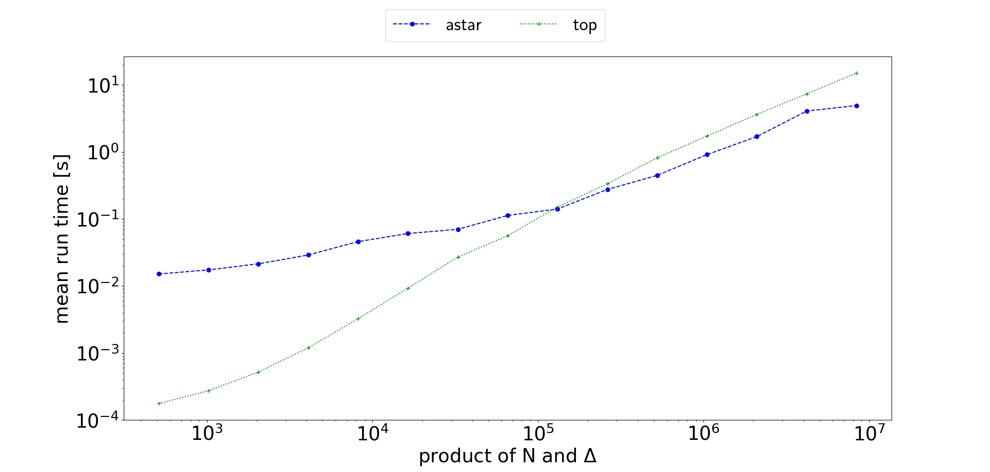
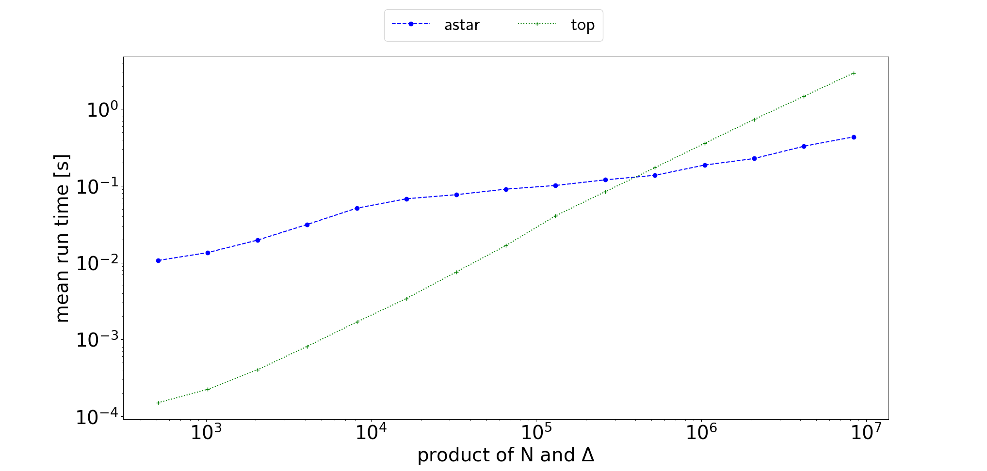
Figure 3: Mean run times of LABEL:itm:top (green, + mark, dotted) and LABEL:itm:astar (blue, circle mark, dashed) over the product of the discretization $N$ and the trust-region radius $\Delta$ for (TR-IP) instances stemming from (SH) (left) and (SR) (right).

We get a similar picture for the overall trend when considering the run times of LABEL:itm:top and LABEL:itm:astar with respect to the number of nodes in the graph. However, the run times do not increase monotonically over the number of nodes in the graph and we observe a sequence of spikes in the run times, which is illustrated in Figure 4. We attribute the dominant spikes in the run times of LABEL:itm:astar to the preprocessing step described in §4.3. The run time of the preprocessing step Algorithm 2 yields an offset for the run time of LABEL:itm:astar, which only depends on $N$ and not on the current trust-region radius $\Delta$.

We also observe a sequence of spikes in the overall run time trend of LABEL:itm:top with respect to the product $N\Delta$. The locations of these spikes seem to be opposed to spikes we observe for LABEL:itm:astar. We attribute these spikes to the fact that if $N$ is relatively large compared to $\Delta$, then the number of edges in the graph is relatively small compared to a graph with a similar value of $N\Delta$, where the ratio $\tfrac{N}{\Delta}$ is smaller.

Figure 4: Mean run times of LABEL:itm:top (green, + mark, dotted) and LABEL:itm:astar (blue, circle, dashed) over the number of nodes in the graphs stemming for (TR-IP) instances stemming from (SH) (left) and (SR) (right).

A closer investigation yields that the run times of LABEL:itm:astar increase less than linearly with respect to $\Delta$. Specifically, LABEL:itm:astar expands only a smaller fraction of the nodes in the graph and larger trust-region radii result in smaller percentages of the nodes being expanded. In particular for the instances generated from (SR), the average percentage of nodes expanded is less than $0.2\%$ for the largest trust-region radius $\Delta=\tfrac{1}{8}N$. We visualize the mean and the 95th percentile of the nodes expanded for different trust-region radii in Figure 5 in §B.

Considering the time required for whole runs of Algorithm 1, we observe a substantial decrease when comparing the runs with LABEL:itm:top and LABEL:itm:astar as subproblem solver to the same runs with LABEL:itm:scip as subproblem solver. The strongest effect can be observed for $N=2048$, the largest case, where the necessary data is fully available. For $N=2048$ and (SH) we observe a decrease of the cumulative run time of the runs of Algorithm 1 from $30200$ s with LABEL:itm:scip to $5242$ s with LABEL:itm:top and $4083$ s with LABEL:itm:astar. Thus the subproblem solves consume $88.4$ % of the run time of Algorithm 1 for LABEL:itm:scip, $32.9$ % for LABEL:itm:top an $13.9$ % for LABEL:itm:astar. For $N=2048$ and (SR) we observe a decrease of the cumulative run time of the runs of Algorithm 1 from $85696$ s with LABEL:itm:scip to $24914$ s with LABEL:itm:top and $24183$ s with LABEL:itm:astar. Thus the subproblem solves consume $76.9$ % of the run time of Algorithm 1 for LABEL:itm:scip, $20.5$ % for LABEL:itm:top an $18.1$ % for LABEL:itm:astar. We have tabulated the cumulative run times of the runs of Algorithm 1 excluding the subproblem solvers over $N$ and $\alpha$ in Table 2 and the cumulative run times of the subproblem solves over $N$ and $\alpha$ for LABEL:itm:astar and LABEL:itm:top in in Tables 3 and 4.

6.3 Choosing the Subproblem Solver Depending on $\Delta$

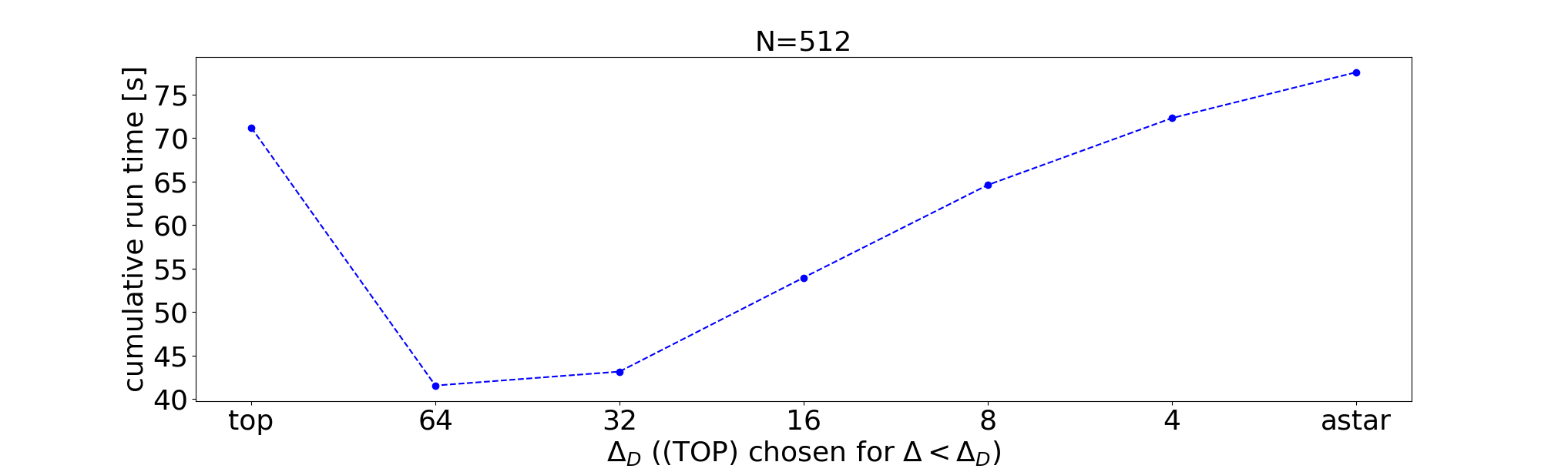
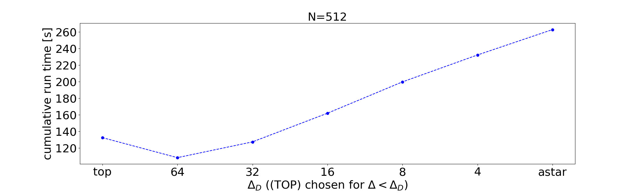
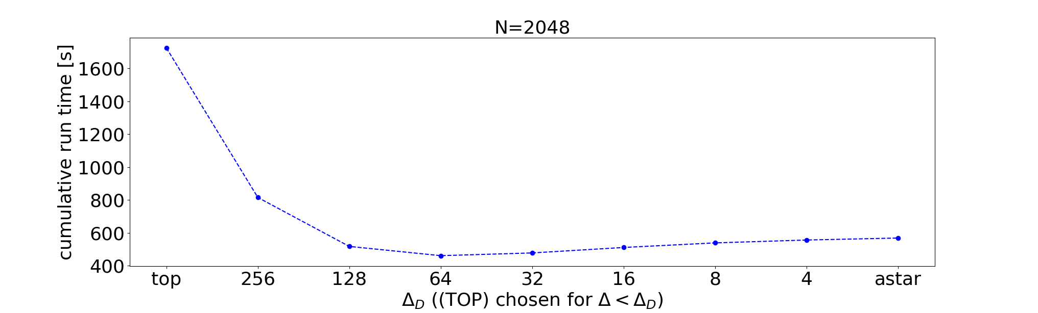
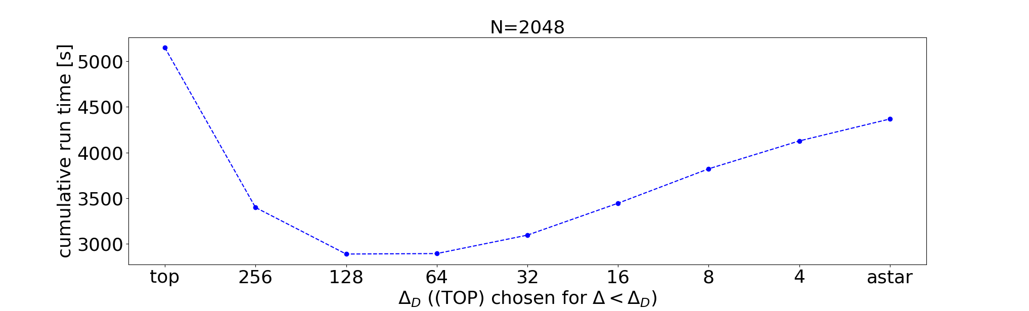
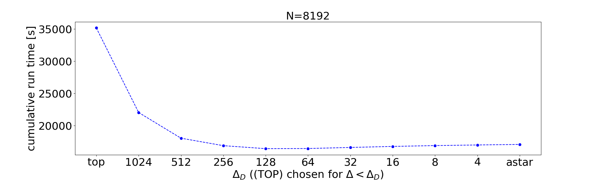
Figure 6: Cumulative run times for the subproblems of the form (TR-IP) stemming from (SH) (left) and (SR) (right) in the runs of Algorithm 1 if one chooses LABEL:itm:top as subproblem solver for $\Delta<\Delta_{D}$ and else LABEL:itm:astar within Algorithm 1.

We choose the subproblem solver in Algorithm 1 depending on the value of $\Delta$. Specifically, we choose LABEL:itm:top if $\Delta$ is less than a decision value $\Delta_{D}$ and LABEL:itm:astar if $\Delta$ is greater than or equal to $\Delta_{D}$. For all values of $N$, we observe that the cumulative run time of the subproblem solves in Algorithm 1 decreases from the value obtained if only LABEL:itm:top is used if $\Delta_{D}$ is decreased until $\Delta_{D}$ is between $64$ and $128$. Then the cumulative run time increases until it reaches the value that is obtained if only LABEL:itm:astar is used ($\Delta_{D}=0$). We visualize the cumulative run times for the subproblem solves of the runs of Algorithm 1 for $N\in\{512,2048,8192\}$ for decreasing values of $\Delta_{D}$ from $\Delta_{D}=\tfrac{1}{4}N$ (only LABEL:itm:top) to $\Delta_{D}=0$ (only LABEL:itm:astar) Figure 6 in §B.

7 Conclusion

We have derived a reformulation of the problem class (TR-IP), which arises as discretized trust-region subproblem in implementations of Algorithm 1, as an RCSPP on an LDAG and as well as a Lagrangian relaxation of the (discretized) trust-region constraint.

The reformulation and the Lagrangian relaxation have lead to a highly efficient $A^{*}$ algorithm that provides optimal solutions and which outperforms on average a general purpose IP solver generally and a topological sorting algorithm on larger problem instances despite having a worse complexity estimate than topological sorting. The average run times per subproblem for both topological sorting and $A^{*}$ are several orders of magnitude lower than those for a general purpose IP solver. We also note that we have observed occasionally that the general purpose IP solver is not able to solve the IP to global optimality within meaningful time limits. Using our $A^{*}$ algorithm or topological sorting allows to overturn the relationship between the run time of the subproblem solves and the other operations in Algorithm 1, mainly the computations of $F(x^{k})$ and $\nabla F(x^{k})$.

We believe that the better performance of $A^{*}$ can be attributed to the fact that the preprocessing and heuristic, both derived from the Lagrangian relaxation, allow to disregard large parts of the underlying graph while the topological sorting always has to process every node and edge in the graph, which is backed by our observation that the percentage of expanded nodes by $A^{*}$ is particularly low if $N$ is large. This observation also leads to a potential further improvement of the run time of Algorithm 1 because we may decide on using topological sorting or $A^{*}$ as subproblem solver depending on the current value of $\Delta$.

Appendix A Tabulated Data of the Numerical Results

Table 1: Number of generated IPs of the form (TR-IP) by the runs of Algorithm 1 on the different discretizations and parameterizations of (SH) (left) and (SR) (right).

	512	1024	2048	4096	8192	Cum.
$10^{-7}$	2055	2960	3692	4645	3878	17230
$10^{-6}$	1727	1291	639	507	1306	5470
$10^{-5}$	310	124	339	524	1018	2315
$10^{-4}$	365	296	427	345	986	2419
$10^{-3}$	303	597	583	675	848	3006
Cum.	4760	5268	5680	6696	8036	30440

	512	1024	2048	4096	8192	Cum.
$10^{-7}$	5382	10026	19026	35294	71696	141424
$10^{-6}$	5142	10713	18821	36514	75515	146705
$10^{-5}$	5119	10101	19526	34843	60932	130521
$10^{-4}$	5199	9202	17737	38816	63021	133975
$10^{-3}$	3899	8875	16291	32812	40859	102736
Cum.	24741	48917	91401	178279	312023	655361

Table 2: Cumulative run times in seconds of Algorithm 1 excluding the run times required for the subproblems of the form (TR-IP) for all instances and start values on the different discretizations and parameterizations of (SH) (left) and (SR) (right).

	512	1024	2048	4096	8192	Cum.
$10^{-7}$	439	1151	2147	3770	4056	11563
$10^{-6}$	450	585	456	429	1299	3219
$10^{-5}$	82	50	219	448	1066	1865
$10^{-4}$	99	137	288	313	1039	1876
$10^{-3}$	91	271	405	598	997	2362
Cum.	1161	2194	3515	5558	8457	20885

	512	1024	2048	4096	8192	Cum.
$10^{-7}$	1175	2206	4109	7774	16455	31719
$10^{-6}$	1135	2353	4075	8075	17166	32804
$10^{-5}$	1127	2220	4224	7744	16691	32006
$10^{-4}$	1143	2011	3852	8569	18260	33835
$10^{-3}$	861	1958	3536	7211	11390	24956
Cum.	5441	10748	19796	39373	79962	155320

Table 3: Cumulative run times in seconds of LABEL:itm:astar for the subproblems of the form (TR-IP) for all instances and start values on the different discretizations and parameterizations of (SH) (left) and (SR) (right).

	512	1024	2048	4096	8192	Cum.
$10^{-7}$	32	97	313	2073	8258	10773
$10^{-6}$	29	52	72	279	2540	2972
$10^{-5}$	5	4	42	251	2378	2680
$10^{-4}$	6	12	58	216	1857	2149
$10^{-3}$	6	26	84	370	2019	2505
Cum.	78	191	569	3189	17052	21079

	512	1024	2048	4096	8192	Cum.
$10^{-7}$	58	210	881	3373	12544	17066
$10^{-6}$	54	224	885	3501	13387	18051
$10^{-5}$	54	211	926	3387	14450	19028
$10^{-4}$	55	192	875	4142	24823	30087
$10^{-3}$	42	184	801	3516	14977	19520
Cum.	263	1021	4368	17919	80181	103752

Table 4: Cumulative run times in seconds of LABEL:itm:top for the subproblems of the form (TR-IP) for all instances and start values on the different discretizations and parameterizations of (SH) (left) and (SR) (right).

	512	1024	2048	4096	8192	Cum.
$10^{-7}$	29	201	1070	5614	18046	24960
$10^{-6}$	28	100	231	612	4859	5830
$10^{-5}$	5	7	98	637	4263	5010
$10^{-4}$	5	23	136	467	3949	4580
$10^{-3}$	5	41	190	836	4028	5100
Cum.	72	372	1725	8166	35145	45480

	512	1024	2048	4096	8192	Cum.
$10^{-7}$	28	192	1061	6798	49089	57168
$10^{-6}$	27	200	1067	6943	50870	59107
$10^{-5}$	27	198	1089	6654	49414	57382
$10^{-4}$	28	177	1007	7153	54746	63111
$10^{-3}$	23	174	925	6232	35243	42597
Cum.	133	941	5149	33780	239362	279365

Table 5: Mean run times in seconds of the solution process for the IPs of the form (TR-IP) for different solution algorithms and problem sizes. The values for the IPs generated by running Algorithm 1 on the different discretizations and parameterizations of (SH) are tabulated left and those of (SR) are tabulated right. The smallest mean run time per value of $N$ is written in bold type. For the algorithm LABEL:itm:scip the mean is computed over all instances (all) for $N\in\{512,1024,2048\}$ and over 50 randomly drawn instances (random) as well as the 50 instances with the highest run time of LABEL:itm:astar (worst) for $N\in\{4096,8192\}$.

N	LABEL:itm:astar	LABEL:itm:top	LABEL:itm:scip
			all	random	worst
512	0.016	0.015	0.511	-	-
1024	0.037	0.071	0.901	-	-
2048	0.100	0.304	4.698	-	-
4096	0.476	1.220	-	209.751	128.430
8192	2.122	4.374	-	56.023	597.785

N	LABEL:itm:astar	LABEL:itm:top	LABEL:itm:scip
			all	random	worst
512	0.011	0.005	0.075	-	-
1024	0.021	0.019	0.223	-	-
2048	0.048	0.056	0.721	-	-
4096	0.101	0.190	-	5.822	9.807
8192	0.227	0.677	-	10.925	309.499

Appendix B Auxiliary Figures Illustrating the Numerical Results

References

- Bestehorn et al., (2019) Bestehorn, F., Hansknecht, C., Kirches, C., and Manns, P. (2019). A switching cost aware rounding method for relaxations of mixed-integer optimal control problems. In 2019 IEEE 58th Conference on Decision and Control (CDC), pages 7134–7139. IEEE.
- Bestehorn et al., (2020) Bestehorn, F., Hansknecht, C., Kirches, C., and Manns, P. (2020). Mixed-integer optimal control problems with switching costs: a shortest path approach. Mathematical Programming, pages 1–32.
- Bestehorn et al., (2021) Bestehorn, F., Hansknecht, C., Kirches, C., and Manns, P. (2021). Switching cost aware rounding for relaxations of mixed-integer optimal control problems: the two-dimensional case. IEEE Control Systems Letters, 6:548–553.
- Bestehorn and Kirches, (2020) Bestehorn, F. and Kirches, C. (2020). Matching algorithms and complexity results for constrained mixed-integer optimal control with switching costs. Optimization Online Preprint. http://www.optimization-online.org/DB_HTML/2020/10/8059.html.
- Cormen et al., (2009) Cormen, T. H., Leiserson, C. E., Rivest, R. L., and Stein, C. (2009). Introduction to Algorithms. MIT Press, 3 edition.
- Dumitrescu and Boland, (2003) Dumitrescu, I. and Boland, N. (2003). Improved preprocessing, labeling and scaling algorithms for the weight-constrained shortest path problem. Networks: An International Journal, 42(3):135–153.
- Gamrath et al., (2020) Gamrath, G., Anderson, D., Bestuzheva, K., Chen, W.-K., Eifler, L., Gasse, M., Gemander, P., Gleixner, A., Gottwald, L., Halbig, K., Hendel, G., Hojny, C., Koch, T., Le Bodic, P., Maher, S. J., Matter, F., Miltenberger, M., Mühmer, E., Müller, B., Pfetsch, M. E., Schlösser, F., Serrano, F., Shinano, Y., Tawfik, C., Vigerske, S., Wegscheider, F., Weninger, D., and Witzig, J. (2020). The SCIP Optimization Suite 7.0. ZIB-Report 20-10, Zuse Institute Berlin.
- Göttlich et al., (2014) Göttlich, S., Kolb, O., and Kühn, S. (2014). Optimization for a special class of traffic flow models: Combinatorial and continuous approaches. Networks & Heterogeneous Media, 9(2):315.
- Göttlich et al., (2017) Göttlich, S., Potschka, A., and Ziegler, U. (2017). Partial outer convexification for traffic light optimization in road networks. SIAM Journal on Scientific Computing, 39(1):B53–B75.
- Habeck et al., (2019) Habeck, O., Pfetsch, M. E., and Ulbrich, S. (2019). Global optimization of mixed-integer ODE constrained network problems using the example of stationary gas transport. SIAM Journal on Optimization, 29(4):2949–2985.
- Hante et al., (2017) Hante, F. M., Leugering, G., Martin, A., Schewe, L., and Schmidt, M. (2017). Challenges in optimal control problems for gas and fluid flow in networks of pipes and canals: From modeling to industrial applications. In Industrial Mathematics and Complex Systems, pages 77–122. Springer.
- Hante and Sager, (2013) Hante, F. M. and Sager, S. (2013). Relaxation methods for mixed-integer optimal control of partial differential equations. Computational Optimization and Applications, 55(1):197–225.
- Haslinger and Mäkinen, (2015) Haslinger, J. and Mäkinen, R. A. (2015). On a topology optimization problem governed by two-dimensional Helmholtz equation. Computational Optimization and Applications, 62(2):517–544.
- Hinze et al., (2008) Hinze, M., Pinnau, R., Ulbrich, M., and Ulbrich, S. (2008). Optimization with PDE constraints, volume 23. Springer Science & Business Media.
- Jung et al., (2015) Jung, M. N., Reinelt, G., and Sager, S. (2015). The Lagrangian relaxation for the combinatorial integral approximation problem. Optimization Methods and Software, 30(1):54–80.
- Kirches et al., (2021) Kirches, C., Manns, P., and Ulbrich, S. (2021). Compactness and convergence rates in the combinatorial integral approximation decomposition. Mathematical Programming, 188(2):569–598.
- Korte and Vygen, (2018) Korte, B. and Vygen, J. (2018). Combinatorial Optimization. Springer, 6 edition.
- Kouri, (2012) Kouri, D. P. (2012). An approach for the adaptive solution of optimization problems governed by partial differential equations with uncertain coefficients.
- Leyffer and Manns, (2021) Leyffer, S. and Manns, P. (2021). Sequential linear integer programming for integer optimal control with total variation regularization. arXiv preprint arXiv:2106.13453.
- Leyffer et al., (2021) Leyffer, S., Manns, P., and Winckler, M. (2021). Convergence of sum-up rounding schemes for cloaking problems governed by the Helmholtz equation. Computational Optimization and Applications, 79(1):193–221.
- Liang and Cheng, (2019) Liang, Y. and Cheng, G. (2019). Topology optimization via sequential integer programming and canonical relaxation algorithm. Computer Methods in Applied Mechanics and Engineering, 348:64–96.
- Liu and Nocedal, (1989) Liu, D. C. and Nocedal, J. (1989). On the limited memory BFGS method for large scale optimization. Mathematical programming, 45(1):503–528.
- Manns, (2021) Manns, P. (2021). Relaxed multibang regularization for the combinatorial integral approximation. SIAM Journal on Control and Optimization, 59(4):2645–2668.
- Manns and Kirches, (2020) Manns, P. and Kirches, C. (2020). Multidimensional sum-up rounding for elliptic control systems. SIAM Journal on Numerical Analysis, 58(6):3427–3447.
- Pearl, (1984) Pearl, J. (1984). Heuristics: Intelligent Search Strategies for Computer Problem Solving. Addison-Wesley Longman Publishing Co., Inc., USA.
- Pfetsch et al., (2015) Pfetsch, M. E., Fügenschuh, A., Geißler, B., Geißler, N., Gollmer, R., Hiller, B., Humpola, J., Koch, T., Lehmann, T., Martin, A., et al. (2015). Validation of nominations in gas network optimization: models, methods, and solutions. Optimization Methods and Software, 30(1):15–53.
- Rathgeber et al., (2016) Rathgeber, F., Ham, D. A., Mitchell, L., Lange, M., Luporini, F., McRae, A. T. T., Bercea, G.-T., Markall, G. R., and Kelly, P. H. J. (2016). Firedrake: automating the finite element method by composing abstractions. ACM Trans. Math. Softw., 43(3):24:1–24:27.
- Sager et al., (2012) Sager, S., Bock, H. G., and Diehl, M. (2012). The integer approximation error in mixed-integer optimal control. Mathematical Programming, 133(1):1–23.
- Sager et al., (2011) Sager, S., Jung, M., and Kirches, C. (2011). Combinatorial integral approximation. Mathematical Methods of Operations Research, 73(3):363–380.
- Sager and Zeile, (2021) Sager, S. and Zeile, C. (2021). On mixed-integer optimal control with constrained total variation of the integer control. Computational Optimization and Applications, 78(2):575–623.
- Svanberg and Werme, (2007) Svanberg, K. and Werme, M. (2007). Sequential integer programming methods for stress constrained topology optimization. Structural and Multidisciplinary Optimization, 34(4):277–299.
- Virtanen et al., (2020) Virtanen, P., Gommers, R., Oliphant, T. E., Haberland, M., Reddy, T., Cournapeau, D., Burovski, E., Peterson, P., Weckesser, W., Bright, J., van der Walt, S. J., Brett, M., Wilson, J., Millman, K. J., Mayorov, N., Nelson, A. R. J., Jones, E., Kern, R., Larson, E., Carey, C. J., Polat, İ., Feng, Y., Moore, E. W., VanderPlas, J., Laxalde, D., Perktold, J., Cimrman, R., Henriksen, I., Quintero, E. A., Harris, C. R., Archibald, A. M., Ribeiro, A. H., Pedregosa, F., van Mulbregt, P., and SciPy 1.0 Contributors (2020). SciPy 1.0: Fundamental Algorithms for Scientific Computing in Python. Nature Methods, 17:261–272.
- Xiao et al., (2005) Xiao, Y., Thulasiraman, K., Xue, G., Jüttner, A., and Arumugam, S. (2005). The constrained shortest path problem: Algorithmic approaches and an algebraic study with generalization. AKCE International Journal of Graphs and Combinatorics, 2.
- Zavala et al., (2010) Zavala, V. M., Wang, J., Leyffer, S., Constantinescu, E. M., Anitescu, M., and Conzelmann, G. (2010). Proactive energy management for next-generation building systems. Proceedings of SimBuild, 4(1):377–385.