Planck constraints on cross-correlations between anisotropic cosmic birefringence and CMB polarization

Abstract

Cosmic Birefringence (CB) is the in-vacuo rotation of the linear polarization direction of photons during propagation, caused by parity-violating extensions of Maxwell electromagnetism. We build low resolution CB angle maps using Planck Legacy and NPIPE products and provide for the first time estimates of the cross-correlation spectra $C_{L}^{\alpha E}$ and $C_{L}^{\alpha B}$ between the CB and the CMB polarization fields. We also provide updated CB auto-correlation spectra $C_{L}^{\alpha\alpha}$ as well as the cross-correlation $C_{L}^{\alpha T}$ with the CMB temperature field. We report constraints by defining the scale-invariant amplitudes $A^{\alpha X}\equiv L(L+1)C_{L}^{\alpha X}/2\pi$, where $X=\alpha,T,E,B$, finding no evidence of CB. In particular, we find $A^{\alpha E}=(-7.8\pm 5.6)$ nK deg and $A^{\alpha B}=(0.3\pm 4.0)$ nK deg at 68% C.L..

1 Introduction

The standard model of particle physics predicts that the electromagnetic (EM) interaction is invariant under the parity operator. Nonetheless, models of parity-violating electromagnetism have been proposed, reflecting the phenomenology of weak interactions [1]. A popular model extends Maxwell’s Lagrangian with a parity-violating Chern-Simons term [2, 3]:

$$\mathcal{L}=\mathcal{L}_{EM}+\mathcal{L}_{CS}=-\dfrac{1}{4}F_{\mu\nu}F^{\mu\nu}-\dfrac{1}{2}p_{\mu}A_{\nu}\widetilde{F}^{\mu\nu},$$ (1.1)

where $F_{\mu\nu}$ is the EM field tensor, $p_{\mu}$ is a constant kinematic four-vector with dimensions of mass, $A_{\nu}$ is the four-potential and $\widetilde{F}^{\mu\nu}=\frac{1}{2}\epsilon^{\mu\nu\alpha\beta}F_{\alpha\beta}$, $\epsilon^{\mu\nu\alpha\beta}$ being the four-dimensional Levi-Civita symbol. The additional parity-violating term $\mathcal{L}_{CS}$ is responsible for the Cosmic Birefringence (CB) effect, the in-vacuo rotation of the linear polarization plane of photons during propagation.

Hence, to observe such an effect one needs a source of linear polarized light. The Cosmic Microwave Background (CMB) is linearly polarized at the level of 1% to 10% due to Thomson scattering off free electrons at the surface of last scattering and it is therefore a good observable to constrain this phenomenon [4, 5]. Moreover, the CMB is the farthest EM radiation available in nature and this increases the chances of detecting the CB effect, as the polarization plane had more time to rotate, since the effect accumulates during propagation.

The CB effect induces correlations between the temperature field T and the B-modes of the polarization field or between the E- and B-modes of the polarization field, that are null with standard EM as the parity symmetry prevents these correlations to be active. Thus, we can use TB and/or EB correlations to detect the CB effect. However, for the Planck data, which are employed in this work, the signal-to-noise ratio due to TB correlation is about a factor of two smaller than EB [6]. Hence, in this paper we focus only on the EB correlation.

If the parity-violating cross-correlations of the CMB fields do not depend on the direction of observation [7, 8, 9, 10, 11, 12, 13, 14, 15, 16], the CB effect is isotropic and it can be modelled with a single angle $\alpha$. Otherwise, the CB effect is anisotropic [17, 18, 19, 20] and it has to be modelled with a set of angles $\alpha(\hat{n})$. Recent constraints on the CB effect can be found in [6, 21, 22, 23, 24, 25, 26, 27] for the isotropic case and in [28, 21, 29, 30] for the anisotropic case. Isotropic and anisotropic CB can be originated by different physical models, see e.g. [31]. In this work, following a phenomenological approach, we focus on the anisotropic case but we also estimate, as consistency check with previous results, the CB monopole, i.e. the isotropic signal.

Parity violating electromagnetism Lagrangian also induce a non-null cross-correlation between the CB field and the CMB temperature and polarization maps, see e.g. [32] and references therein for a detailed treatment of cross-spectra and bi-spectra. Furthermore, in recent years, early dark energy models inspired by ultra-light axion fields [33, 34] have been proposed to alleviate the $H_{0}$ tension [35]. These models are known to produce CB signal and a non-zero cross-correlation between CB and the CMB fields, see e.g. [36].

In this paper we analyze CB extending what was done in Ref. [21]. In particular, using the Planck Public Data Release 3 (PR3) products, we provide for the first time constraints on the cross-correlation spectra $C_{L}^{\alpha E}$ and $C_{L}^{\alpha B}$ between the CB angle maps and the CMB polarization maps at large angular scales. We also provide the CB auto-correlation spectra $C_{L}^{\alpha\alpha}$ and its cross-correlation spectra $C_{L}^{\alpha T}$ with the CMB temperature map up to $L=24$, exploiting the Planck Public Data Release 4 (NPIPE) data in addition to the Planck PR3 products.

This paper is organized as follows: in Section 2 we review the features of the Planck datasets and simulations employed for this study; in Section 3 we describe the analysis pipeline; in Section 4 we present the results of this work; in Section 5 we draw the conclusions; in Appendix A we discuss the purification of E and B modes for the CMB Angular Power Spectra (APS) estimation; in Appendix B we explain the effective beam calculation used for the CMB spectra; in Appendix C we report the results of the analysis on simulations; in Appendix D we perform robustness tests for the analysis pipeline; in Appendix E we set 2-dimensional (2D) joint constraints on $A^{\alpha\alpha}$ and $A^{\alpha T}$.

2 Datasets and Simulations

In this work we employ CMB maps provided by the Planck collaboration in the PR3 analysis [37] and in the subsequent NPIPE re-analysis [38]. The PR3 maps have been cleaned from foregrounds by the four official Planck component separation methods Commander, NILC, SEVEM and SMICA [39], while NPIPE maps have been processed only by Commander and SEVEM [38]. The corresponding simulations, provided by the Planck collaboration, have been also employed. The resolution of the maps, following the HEALPix [40] pixelization scheme, is $N_{side}=2048$. The NPIPE products have never been used to estimate the CB auto-correlation spectra $C_{L}^{\alpha\alpha}$ before this work.

The PR3 simulation set is composed of 1000 CMB Monte Carlo simulations generated using the Planck $\Lambda$CDM best-fit model, 300 noise simulations for the full-mission (FM) and 300 noise simulations for each of the two half-mission (HM) data splits, and for each of the component separation methods. We sum the first 300 CMB realizations with each set of 300 HM noise simulations that realistically describe the Planck 2018 data. We employ the two data splits in the construction of the $\alpha$ map. We also sum the first 300 CMB realizations with the 300 FM noise simulations in order to obtain 300 FM simulations. We use these maps for the cross-correlation spectra $C_{L}^{\alpha E}$ and $C_{L}^{\alpha B}$ estimation. The PR3 simulations contain beam leakage effects [41], ADC non linearities, thermal fluctuations and other systematic effects [42].

The NPIPE data and simulation sets are an evolution over PR3 [38]. One of the effects of these improvements is lower levels of noise and systematics in the CMB maps at essentially all angular scales [38]. We employ the 400 simulations available for Commander and the 600 simulations available for SEVEM. The NPIPE Commander simulations contain the PR3 CMB signal and the instrumental noise. To extract the noise-only maps, we subtract the signal-only PR3 simulations to the complete NPIPE simulations. The NPIPE SEVEM CMB simulations are divided in noise-only and signal-only as the PR3 ones, which we sum for a set of noisy CMB simulations. The NPIPE data splits, where the systematics between the splits are expected to be uncorrelated, are called A and B (see again [38] for a full description). We calculate the NPIPE CMB APS by cross-correlating those A and B maps. The NPIPE simulations employed in this work are the “noise aligned” ones, see again [38] for details.

3 Analysis pipeline

As first step of the analysis we need to define the processing masks. We divide the HEALPix sky at $N_{side}=2048$ in small regions following the pixelization scheme at $N_{side}=8$. In the rest of the paper we refer to these regions as “patches”. The sky fraction covered by one single patch is $f_{sky,patch}\simeq 0.13\%$ and the total number of available patches is 768. Working at resolution $N_{side}=8$ is an improvement with respect to [21], where they used $N_{side}=4$. We tried to increase the resolution to $N_{side}=16$, but the patch sky fraction was too low to get reliable CMB spectra.

We then combine the masks of these patches with a polarization mask that excludes the regions unobserved or heavily contaminated by foregrounds. For PR3 we combine the foreground mask (Galactic and point sources) with the HM missing pixels mask. For NPIPE only the foreground mask is employed. The polarization masks used are shown in the top panels of Fig. 1 (left for PR3, right for NPIPE).

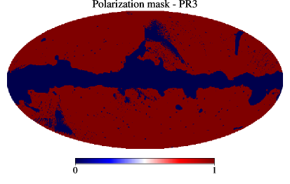
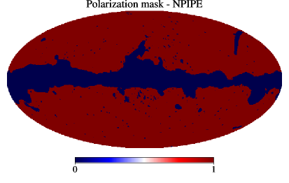
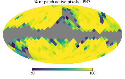
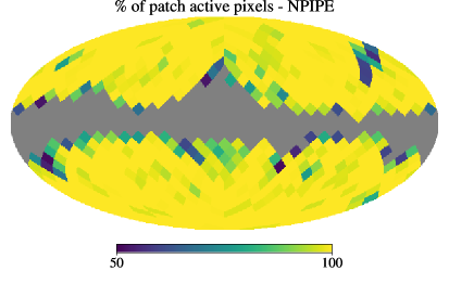
Figure 1: Top: polarization masks used in this work (left for PR3, right for NPIPE). Bottom: percentage of active pixels in each patch (left for PR3, right for NPIPE). The grey patches are not used in the analysis. The patches marked with a red x in the bottom left panel are the ones whose CMB spectra validation is shown in Fig. 2, i.e. patches with HEALPix indexes 1, 207, 542 from top to bottom.

Some of the aforementioned patches contain masked pixels. A large fraction of masked pixels in a patch prevents the extraction of reliable CMB spectra. For this reason, we select and analyze only the patches that have at least 50% of active (i.e. non masked) pixels. This corresponds to $f_{sky,patch}\gtrsim 0.065\%$. The maps showing the selected patches and the fraction of active pixels in each of them are shown in the bottom panels of Fig. 1 (left for PR3, right for NPIPE), where the grey patches are the excluded ones. As expected, among the selected patches, the ones close to the Galactic mask borders or the ones containing a large number of point sources have a lower percentage of active pixels. The number of selected patches is 571 for PR3 and 592 for NPIPE. The final masks are not apodized because the apodization process reduces the effective sky fraction covered by each patch and, for the sky fraction considered, it does not provide any benefit in the CMB computed APS, see also the discussion about polarization purification in the next paragraph.

For each selected patch, the CMB APS is calculated with the Python package Pymaster [43] by cross-correlating the two splits both for data and simulations. We recall that the data splits are HM 1 and 2 for PR3, A and B for NPIPE, as explained in Sec. 2. We compute the APS in cross-mode to reduce systematic effects and noise mismatches [44, 42]. When analysing a masked CMB map to produce the APS, E to B leakage can be generated [45]. We have the possibility to purify the E and/or B modes in order to remove the misinterpreted modes, at a cost of information loss [45, 43]. We choose not to purify E and B modes: for the noise level of Planck, the size of the patches considered and for the multipole range of interest, the purification does not provide any substantial advantage, and does increase the error bars (see App. A for more details). We calculate the APS for multipoles from 2 to 2047. We deconvolve a non-Gaussian effective beam obtained from simulations, as explained in App. B. The APS is binned with $\Delta l=60$ multipoles in order to reduce the errors and the correlations induced by the cut-sky [46].

We show in the top panels of Fig. 2 the PR3 Commander validation plots for the EE, BB and EB power spectra for three patches, in terms of the bandpowers $D_{\ell}=\ell(\ell+1)C_{\ell}/2\pi$.

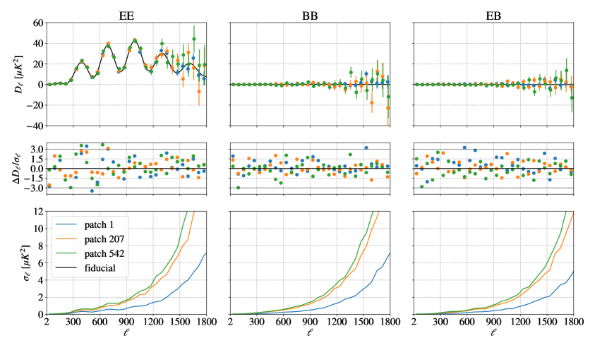
Figure 2: Top: EE (left), BB (center) and EB (right) CMB power spectra for three patches and for the Commander component separation method. The black line represents the fiducial, while the blue, orange and green points are the simulation average spectra for the patches with HEALPix RING ordering indexes 1, 207 and 542, respectively (highlighted with a red cross in Fig. 1). The error bars represent the error of the mean. Center: EE, BB and EB difference between the simulation average and the fiducial spectra, divided by the error of the mean. Bottom: EE, BB and EB errors of the mean.

The three patches, following the HEALPix RING ordering scheme, have indexes 1 (blue), 207 (orange) and 542 (green) and fractions of patch active pixels 100%, 74.5% and 51.1%, respectively. The dots represent the mean of the simulations and the error bars show the uncertainty on the mean. The fiducial power spectra are represented by the black lines in the plots. These plots show that the simulations CMB spectra are validated. The scatter around the fiducial at the highest multipoles is large and, for this reason, we do consider the APS with $\ell\lesssim 1500$. We show in the central panels of Fig. 2 the residuals plots, i.e. the difference between the simulation average and the fiducial spectra, divided by the error of the mean. For all the cases considered the simulation average is less than $3.5\sigma_{\rm mean}$ away from the fiducial. The residuals do not show any systematic behaviour. We report in the bottom panels of Fig. 2 the error of the mean. As expected, the error increases for higher multipoles and for lower numbers of active pixels in the patch. We verified that the behaviour of other patches and other component separation methods is similar to the one shown in Fig. 2. For the NPIPE case the simulations are validated with a similar procedure, the only difference is that the errors are slightly smaller. This is due to the lower level of noise with respect to the PR3 simulation set [38].

Given the low number of simulations, the CMB covariance matrices for each patch and for each component separation method are obtained via the analytical implementation of Pymaster [43]. The module that produces the matrices needs the CMB signal APS, the noise APS and the smoothing function. The CMB signal APS used for the covariance matrix calculation is the Planck FFP10 fiducial [42]. The noise APS for each of the two data splits (HM1 and HM2 for PR3, A and B for NPIPE) is obtained by averaging the auto-correlation of the corresponding noise-only simulations. The smoothing function considered is obtained as discussed in App. B. We verified that these analytical covariance matrices are a good approximation of the ones obtained using the simulations. This is not valid for the first multipole bin, so we exclude the latter from the analysis and use the CMB spectra starting from $\ell_{min}=62$.

After obtaining the CMB APS and the corresponding covariance matrices, we estimate the CB angle in each patch assuming that the CB effect is isotropic inside each patch. The CMB APS is rotated by the isotropic CB effect in the following way [16]:

$$C_{\ell}^{TT,obs} =C_{\ell}^{TT},$$ (3.1)

$$C_{\ell}^{TE,obs} =C_{\ell}^{TE}\cos(2\alpha),$$ (3.2)

$$C_{\ell}^{TB,obs} =C_{\ell}^{TE}\sin(2\alpha),$$ (3.3)

$$C_{\ell}^{EE,obs} =C_{\ell}^{EE}\cos^{2}(2\alpha)+C_{\ell}^{BB}\sin^{2}(2\alpha),$$ (3.4)

$$C_{\ell}^{BB,obs} =C_{\ell}^{BB}\cos^{2}(2\alpha)+C_{\ell}^{EE}\sin^{2}(2\alpha),$$ (3.5)

$$C_{\ell}^{EB,obs} =\frac{1}{2}\left(C_{\ell}^{EE}-C_{\ell}^{BB}\right)\sin(4\alpha),$$ (3.6)

where $\alpha$ is the CB angle, the APS with the $obs$ tag is the rotated (observed) one and the APS without the $obs$ tag is the unrotated one. Without the CB effect, i.e. $\alpha=0$, the TB and EB spectra are null, as expected.

Harmonic based estimators for $\alpha$ can be built exploiting the observed EB and/or TB spectra, see e.g. [16]. Since the signal-to-noise ratio is smaller for the TB-based estimator as compared to EB one, we use the EB-only D-estimator defined in [16]:

$$D_{\ell}^{EB,obs}=C_{\ell}^{EB,obs}\cos(4\alpha)-\frac{1}{2}\left(C_{\ell}^{EE,obs}-C_{\ell}^{BB,obs}\right)\sin(4\alpha)\thinspace.$$ (3.7)

We obtain an estimate of the isotropic CB angle $\alpha$ in each patch by minimizing the following $\chi^{2}_{EB}$:

$$\chi^{2}_{EB}=\sum_{\ell,\ell^{\prime}}D_{\ell}^{EB,obs}M_{\ell\ell^{\prime}}^{EB}D_{\ell^{\prime}}^{EB,obs},$$ (3.8)

where $D_{\ell}^{EB,obs}$ are the D-estimators defined in Eq. (3.7) and $M_{\ell\ell^{\prime}}^{EB}=\langle D_{\ell}^{EB,obs}D_{\ell^{\prime}}^{EB,obs}\rangle^{-1}$ is their covariance matrix. The $M_{\ell\ell^{\prime}}^{EB}$ matrix reduces to the EB covariance matrix, i.e. without the CB effect [16], when the noise on the E and B CMB fields is equivalent. Since the latter is valid for the Planck maps we are employing [44, 42], we use the EB covariance matrix in the $\chi^{2}_{EB}$ minimization. Only the CMB spectra and covariance matrix related to a specific patch are used in the $\chi^{2}_{EB}$ to estimate the CB angle in that patch.

For each CMB map we minimize the $\chi^{2}_{EB}$ in each patch obtaining a map of CB angles. From these maps we firstly estimate the CB monopole averaging the angle values in the pixels outside the masks shown in the bottom panels of Fig. 1. Then, we calculate their auto-correlation spectra $C_{L}^{\alpha\alpha}$ and their cross-correlation spectra $C_{L}^{\alpha T}$, $C_{L}^{\alpha E}$ and $C_{L}^{\alpha B}$ with the CMB T, Q, U maps employing a Quadratic Maximum Likelihood (QML) estimator [47, 48, 49, 50], where $\alpha$ represents an extra scalar field. The maps and the associated covariance matrices used in the QML estimator are described in the next paragraphs.

The CB fields for data and simulations are obtained through the $\chi^{2}_{EB}$ minimization, described above. Following [21], the covariance matrices associated to the data are assumed to be diagonal, and they are computed from the variance of the simulations in each pixel. See App. C for more details about this choice. In the computation of the angular power spectra, we marginalize over monopole (for all the cases) and dipole (for the $\alpha T$, $\alpha E$ and $\alpha B$ cases) contributions following the procedure described in [51, 52]. Hence, note that we retain $L=1$ as the lowest multipole for $\alpha\alpha$ spectra.

For the CMB temperature field we always use the Commander map since it is the one used by the Planck collaboration for the large scale temperature cosmological analysis. We produce 300 signal-only CMB temperature simulations at HEALPix resolution $N_{side}=8$ smoothed with a Gaussian beam with 880’ FWHM and an analytic pixel window function, to which we sum isotropic white noise realizations with standard deviation of 500 nK for regularization. The Commander data map is down-sampled and regularized accordingly. The CMB temperature covariance matrix is analytically calculated from the FFP10 fiducial spectrum [42] and contains the marginalization of monopole and dipole and a diagonal term to take into account the 500 nK regularization noise.

For the CMB polarization fields, instead, we use the SMICA polarization maps because it is the only component separation method providing harmonic weights [39, 53] that allow to correctly compute the pixel space noise covariance matrix, from single frequency noise covariances. We down-sample the 300 PR3 polarization simulations and the data maps from $N_{side}=2048$ to $N_{side}=8$, applying, in addition to an analytic pixel window function, a cosine window function [54] defined as:

$$b_{\ell}=\left\{\begin{matrix}1&\mbox{for $\ell<N_{side}$}\\ \frac{1}{2}\left(1+\sin\left(\frac{\pi}{2}\frac{\ell}{N_{side}}\right)\right)&\hskip 20.0pt\mbox{for $N_{side}\leq\ell<3\ N_{side}$}\\ 0&\mbox{otherwise}\\ \end{matrix}\right..$$ (3.9)

We then sum a 20 nK regularization noise. The corresponding covariance matrix contains: the correlated noise term (computed using the SMICA weights and the FFP8 [41] noise covariance matrices), the signal term based on a fiducial power spectrum, and the regularization noise term. We limit the estimates of the $\alpha E$ and $\alpha B$ spectra at $L=23$ by definition of the considered smoothing window.

We show in Fig. 3 the masks used for the extraction of the spectra with the QML estimator. The mask employed with the $\alpha$ and $T$ maps has $\approx$ 74% of non-masked pixels, while the fraction of active pixels for the $Q$ and $U$ mask is $\approx$ 47%. The masks are obtained as the product of the PR3 $\alpha$ mask, that excludes the grey patches shown in the bottom left panel of Fig. 1, and the CMB galactic mask for intensity ($\alpha$ and $T$ maps) or polarization ($Q$ and $U$ maps).

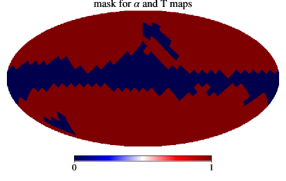
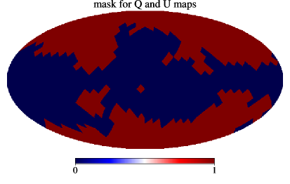
Figure 3: Masks used for the CB spectra QML estimator for the $\alpha$ and $T$ (left), $Q$ and $U$ (right) maps.

After having obtained the $C_{L}^{\alpha X}$ spectra, where X can be $\alpha$, T, E or B, we set constraints in terms of the scale-invariant amplitude $A^{\alpha X}$. To do so, we minimize the following $\chi^{2}\left(A^{\alpha X}\right)$:

$$\chi^{2}\left(A^{\alpha X}\right)=\sum_{L,L^{\prime}}\left(\dfrac{L(L+1)}{2\pi}C_{L}^{\alpha X}-A^{\alpha X}\right)M_{LL^{\prime}}^{-1}\left(\dfrac{L^{\prime}(L^{\prime}+1)}{2\pi}C_{L^{\prime}}^{\alpha X}-A^{\alpha X}\right),$$ (3.10)

where $C_{L}^{\alpha X}$ are the data spectra and $M_{LL^{\prime}}=\left<\dfrac{L(L+1)}{2\pi}C_{L}^{\alpha X}\dfrac{L^{\prime}(L^{\prime}+1)}{2\pi}C_{L^{\prime}}^{\alpha X}\right>$ is calculated from simulations.

4 Results

In this section we show the results of our analysis, adopting the following color code: red for Commander, orange for NILC, green for SEVEM, and blue for SMICA.

In Figure 4 we show the CB maps (left panels) extracted from CMB data, and the associated error maps computed from simulations (right panels) for the PR3 dataset. In Figure 5 the same quantities are displayed for NPIPE.

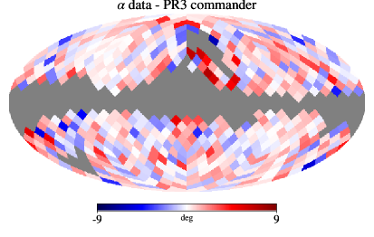
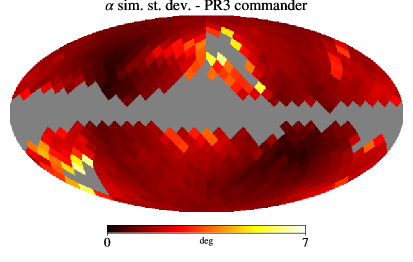
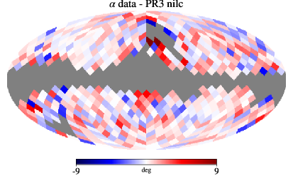
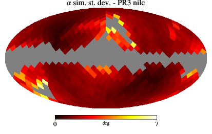
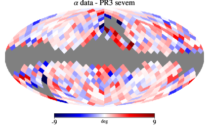
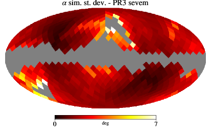
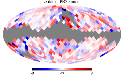
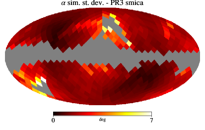
Figure 4: Cosmic Birefringence angle maps obtained from the PR3 polarization maps for the Commander, NILC, SEVEM and SMICA component separation methods (from top to bottom). Left: data. Right: standard deviation of simulations.

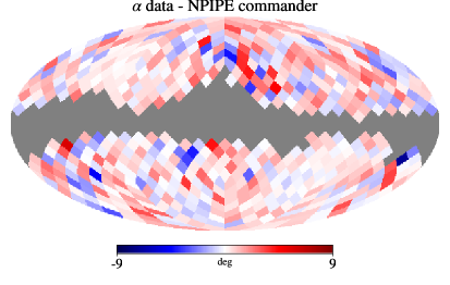
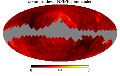
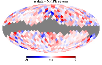
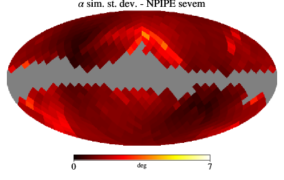
Figure 5: Cosmic Birefringence angle maps obtained from the NPIPE polarization maps for the Commander and SEVEM component separation methods (from top to bottom). Left: data. Right: standard deviation of simulations.

By visually comparing PR3 CB maps, we can recognize similar patterns for all the four component separation methods. The same applies to the NPIPE dataset. The errors associated to NPIPE are generally lower with respect to the PR3 ones. This is simply due to the fact that the NPIPE CMB maps are slightly less noisy than the PR3 ones [38]. Furthermore some NPIPE low resolution patches contain a larger number of observed pixels, with respect to the PR3 dataset, whose mask contains also the contribution of half mission missing pixels (see top panels of Fig. 1). Finally, the darker regions in error maps, which represent patches where the error on the CB angle is lower, are well correlated with the Planck scanning strategy [55], that observes more deeply the ecliptic poles.

case	$\bm{\alpha\ \mathrm{[deg]}}$
PR3 Commander	$\mathrm{0.27\pm 0.05\ (stat)\pm 0.28\ (syst)}$
PR3 NILC	$\mathrm{0.26\pm 0.05\ (stat)\pm 0.28\ (syst)}$
PR3 SEVEM	$\mathrm{0.27\pm 0.05\ (stat)\pm 0.28\ (syst)}$
PR3 SMICA	$\mathrm{0.24\pm 0.05\ (stat)\pm 0.28\ (syst)}$
NPIPE Commander	$\mathrm{0.33\pm 0.04\ (stat)\pm 0.28\ (syst)}$
NPIPE SEVEM	$\mathrm{0.33\pm 0.04\ (stat)\pm 0.28\ (syst)}$
[23] (PR3)	$\mathrm{0.35\pm 0.14\ (stat)}$
[24] (NPIPE)	$\mathrm{0.30\pm 0.11\ (stat)}$
[26] (NPIPE + WMAP)	$\mathrm{0.30^{+0.094}_{-0.091}\ (stat)}$

Table 1: Monopole of the data CB angle maps produced in this work. The values found in [23], [24], and [26] are also reported for reference.

In Table 1 we report the monopoles of the CB maps. They are obtained as a weighted average of the data maps with weights corresponding to the inverse variance of the simulations. All the monopole values are consistent with zero provided the systematic error is taken into account. Moreover they are well compatible, within the statistical uncertainty, across the different component separation methods. The statistical error contribution is computed from the standard deviation of the simulations, while the systematic error is due to the uncertainty in the orientation of Planck’s polarization-sensitive bolometers [56] and is taken from Ref. [6]. Also here we note that, due to the lower level of the instrumental noise [38] and to the larger number of non-masked pixels, the NPIPE data provide smaller statistical errors. The monopole values found in this work agree with the ones reported in literature, see e.g. [6, 21, 22, 23, 24, 26].

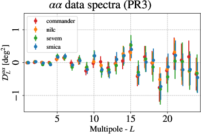
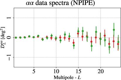
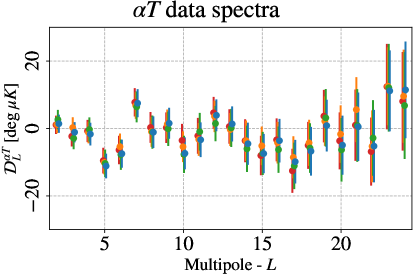
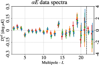
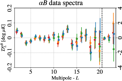
Figure 6: Auto-correlation spectra of the data CB angle maps and their cross-correlation with CMB. The errors are the standard deviations of the simulations. The vertical dashed lines highlight a change in the vertical axis range. Top left panel: PR3 $\alpha\alpha$. Top right panel: NPIPE $\alpha\alpha$. Central panel: PR3 $\alpha T$. Bottom left panel: PR3 $\alpha E$. Bottom right panel: PR3 $\alpha B$.

In Figure 6 we show the auto-correlation of the CB maps and their cross-correlation with CMB. As expected the scatter of the NPIPE $\alpha\alpha$ spectra around zero and the associated errors are slightly lower with respect to PR3. Across the spectra, we find a general good compatibility with the null effect. This is assessed by comparing the harmonic $\chi^{2}$ of data and simulations, reported in Fig. 7.

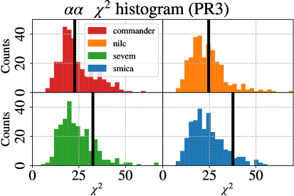
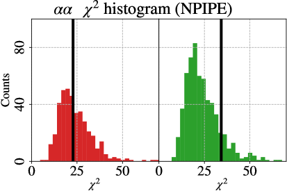
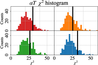
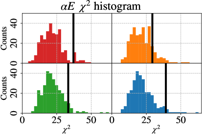
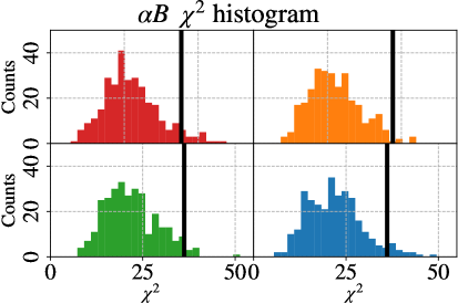
Figure 7: Harmonic $\chi^{2}$ plots (histogram for simulations, black line for data). Top left panel: PR3 $\alpha\alpha$. Top right panel: NPIPE $\alpha\alpha$. Central panel: PR3 $\alpha T$. Bottom left panel: PR3 $\alpha E$. Bottom right panel: PR3 $\alpha B$.

The data $\chi^{2}$ for all the spectra lies within the histograms, suggesting that the data are compatible with the simulations, hence with the null effect. However, we note that for the $\alpha E$ and $\alpha B$ cases the $\chi^{2}$ of the data are closer to the right tail of the corresponding histograms, with the following Probability To Exceed (PTE): 0.9–10.6% for $\alpha E$ and 1.4–2.5% for $\alpha B$ (see also Tab. 2 where all the PTEs are reported).

case	Commander	NILC	SEVEM	SMICA
$\alpha\alpha$ PR3	47.6%	37.1%	9.0%	2.8%
$\alpha\alpha$ NPIPE	47.1%	-	6.2%	-
$\alpha T$ PR3	10.9%	27.4%	23.6%	7.5%
$\alpha E$ PR3	1.6%	10.6%	4.2%	0.9%
$\alpha B$ PR3	2.5%	1.4%	2.1%	2.1%

Table 2: Probability To Exceed obtained from the harmonic $\chi^{2}$ reported in Fig. 7.

Despite the overall good compatibility with the null effect, some single multipole fluctuations deserve a closer look. Considering the $\alpha T$ spectra, $L=5$ shows a PTE between 1% and 2.7% for the four component separation methods, i.e. $\sim 2.5\sigma$ fluctuation. For the $\alpha E$ spectra, the multipoles $L=5,12,14,19$ have the largest deviation from the null effect, if compared with the corresponding empirical distributions. These PTEs are below 1% for $D_{19}^{\alpha E}$ Commander and $D_{12}^{\alpha E}$ SEVEM, but still within $3\sigma$ fluctuation. The same happens for $D_{2}^{\alpha B}$ NILC, SEVEM and SMICA, all with PTEs lower than 1%, but within $3\sigma$. The PTE for $D_{13}^{\alpha B}$ is between 2% and 2.7%, which corresponds to $\sim 2.3\sigma$ fluctuation. All the spectra obtained with the SMICA component separation method are reported in Tab. 3 along with the statistical uncertainty at $1\sigma$ level for each multipole. The averaged spectra of the simulations are shown in App. C. They all show a nice compatibility with the null-hypothesis, meaning that the residual systematic effects included in the simulations do not have a significant impact on the spectra considered.

$\bm{L}$	$\bm{D_{L}^{\alpha\alpha}[deg^{2}]}$	$\bm{D_{L}^{\alpha T}[\mu K\ deg]}$	$\bm{D_{L}^{\alpha E}[\mu K\ deg]}$	$\bm{D_{L}^{\alpha B}[\mu K\ deg]}$
1	$-0.004\pm 0.006$	-	-	-
2	$\phantom{-}0.026\pm 0.019$	$\phantom{-}1.404\pm 2.683$	$\phantom{-}0.027\pm 0.021$	$\phantom{-}0.048\pm 0.016$
3	$-0.013\pm 0.028$	$-1.123\pm 2.996$	$\phantom{-}0.040\pm 0.025$	$\phantom{-}0.013\pm 0.013$
4	$-0.063\pm 0.049$	$-1.678\pm 3.351$	$\phantom{-}0.013\pm 0.024$	$-0.032\pm 0.015$
5	$\phantom{-}0.166\pm 0.060$	$-11.140\pm 3.668$	$-0.054\pm 0.026$	$-0.022\pm 0.014$
6	$\phantom{-}0.194\pm 0.083$	$-7.479\pm 4.151$	$-0.006\pm 0.022$	$\phantom{-}0.011\pm 0.014$
7	$-0.074\pm 0.090$	$\phantom{-}7.492\pm 4.141$	$-0.013\pm 0.021$	$-0.001\pm 0.016$
8	$\phantom{-}0.058\pm 0.112$	$-1.114\pm 4.663$	$-0.018\pm 0.022$	$-0.002\pm 0.018$
9	$-0.211\pm 0.137$	$\phantom{-}1.536\pm 4.577$	$-0.001\pm 0.023$	$-0.010\pm 0.019$
10	$\phantom{-}0.206\pm 0.135$	$-7.389\pm 4.740$	$-0.035\pm 0.023$	$\phantom{-}0.020\pm 0.019$
11	$-0.215\pm 0.169$	$-3.359\pm 5.139$	$\phantom{-}0.016\pm 0.025$	$-0.014\pm 0.023$
12	$-0.294\pm 0.188$	$\phantom{-}3.900\pm 4.707$	$-0.062\pm 0.028$	$\phantom{-}0.027\pm 0.025$
13	$\phantom{-}0.097\pm 0.224$	$\phantom{-}1.340\pm 5.185$	$-0.041\pm 0.029$	$\phantom{-}0.057\pm 0.024$
14	$\phantom{-}0.213\pm 0.253$	$-4.532\pm 6.245$	$\phantom{-}0.087\pm 0.034$	$-0.046\pm 0.031$
15	$\phantom{-}0.399\pm 0.266$	$-7.444\pm 5.834$	$-0.045\pm 0.038$	$-0.055\pm 0.031$
16	$-0.373\pm 0.307$	$-3.625\pm 6.447$	$-0.034\pm 0.039$	$\phantom{-}0.002\pm 0.037$
17	$\phantom{-}0.015\pm 0.298$	$-9.853\pm 6.462$	$-0.017\pm 0.045$	$\phantom{-}0.021\pm 0.039$
18	$\phantom{-}0.071\pm 0.357$	$-6.756\pm 7.213$	$-0.033\pm 0.049$	$-0.098\pm 0.050$
19	$-0.729\pm 0.403$	$\phantom{-}0.848\pm 7.662$	$\phantom{-}0.095\pm 0.065$	$\phantom{-}0.042\pm 0.064$
20	$-0.131\pm 0.406$	$-4.962\pm 8.737$	$-0.000\pm 0.095$	$\phantom{-}0.039\pm 0.093$
21	$\phantom{-}0.221\pm 0.450$	$\phantom{-}0.500\pm 10.144$	$\phantom{-}0.106\pm\phantom{-}0.163$	$-0.104\pm 0.149$
22	$-0.218\pm 0.497$	$-5.240\pm 10.748$	$-0.241\pm 0.365$	$\phantom{-}0.024\pm 0.338$
23	$-0.209\pm 0.476$	$\phantom{-}11.141\pm 11.989$	$-0.213\pm 1.477$	$\phantom{-}0.526\pm 1.429$
24	$-0.455\pm 0.470$	$\phantom{-}11.452\pm 14.336$	-	-

Table 3: CB spectra for the PR3 SMICA case. The $\alpha E$ and $\alpha B$ spectra are calculated up to $L=23$ as the $coswin$ smoothing (and thus the spectra) are null for higher multipoles, as discussed in Sec. 3.

In Figure 8 we display the posterior distributions for the scale invariant amplitude, $A^{\alpha X}$, computed using Eq. (3.10). In Table 4 we report the upper limits at 95% C.L., for $A^{\alpha\alpha}$, and the constraints at 68% C.L., for $A^{\alpha T}$, $A^{\alpha E}$ and $A^{\alpha B}$. As before, also for these parameters, we find a good compatibility among the different component separation methods and with the null effect. Furthermore, for $A^{\alpha\alpha}$, there is good compatibility between the PR3 and the NPIPE results. The NPIPE upper limit using the Commander component separation method is looser with respect to the PR3 one because the posterior peak is slightly shifted to the right. Even if a small shift is present also for SEVEM, the lower width of the posterior of NPIPE results in a tighter constraint on $A^{\alpha\alpha}$, when compared with SEVEM PR3. The $\alpha T$ constraints are compatible with, but tighter than [21], where they used the same approach adopted in this work but at the lower resolution $N_{side}=4$. Thus, a higher resolution provides more constraining power for $\alpha T$.

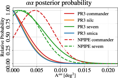
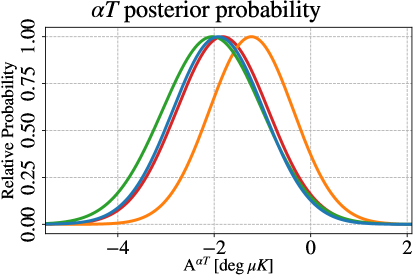
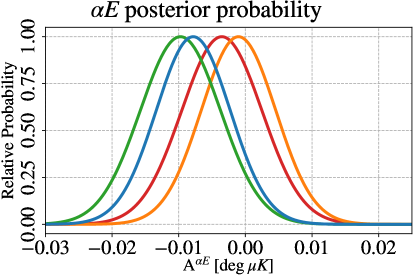
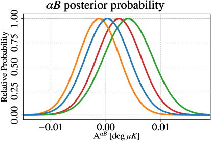
Figure 8: Posteriors for the scale invariant spectrum fit. Top left panel: PR3 and NPIPE $\alpha\alpha$. Top right panel: PR3 $\alpha T$. Bottom left panel: PR3 $\alpha E$. Bottom right panel: PR3 $\alpha B$.

parameter	Commander	NILC	SEVEM	SMICA
$\mathrm{A^{\alpha\alpha}\ [deg^{2}]\ PR3}$	$<0.007$	$<0.007$	$<0.010$	$<0.007$
$\mathrm{A^{\alpha\alpha}\ [deg^{2}]\ NPIPE}$	$<0.010$	-	$<0.009$	-
$\mathrm{A^{\alpha T}\ [\mu K\ deg]\ PR3}$	$-1.827\pm 0.953$	$-1.229\pm 0.873$	$-2.037\pm 1.038$	$-1.916\pm 0.945$
$\mathrm{A^{\alpha E}\ [nK\ deg]\ PR3}$	$-3.5\pm 6.0$	$-1.0\pm 5.6$	$-9.7\pm 6.0$	$-7.8\pm 5.6$
$\mathrm{A^{\alpha B}\ [nK\ deg]\ PR3}$	$\hphantom{-}2.4\pm 4.0$	$-1.2\pm 3.7$	$\hphantom{-}4.0\pm 4.4$	$\hphantom{-}0.3\pm 4.0$

Table 4: Constraints on the scale invariant power spectrum $A^{\alpha X}$, with $X=\alpha,T,E,B$, set in this work.

5 Conclusions

In this work we build CB maps at angular scales larger than $\sim 7$ deg, exploiting Planck CMB component separated maps from both PR3 and NPIPE releases. From these CB maps we estimate the monopoles (see Tab. 1), i.e. the isotropic birefringence angle, finding a very good compatibility with previous results [6, 21, 22, 23, 24]. We also compute their spectra and the cross-correlation with the CMB temperature map. Moreover, we provide for the first time the spectra of the cross-correlation of the CB field with the CMB E and B fields. The data CB angle maps and spectra, for both auto- and cross-correlations with CMB, are made publicly available.

We quantify the compatibility of all the aforementioned spectra with null effect through an harmonic $\chi^{2}$ analysis, see Fig. 7, and through a scale invariant amplitude $A^{\alpha X}$, with $X=\alpha,T,E,B$, see Fig. 8. We find no significant evidence of deviation from the null effect. The constraints on $A^{\alpha X}$ are summarized in Tab. 4. The latter are obtained through a $\chi^{2}$ minimization assuming null CB, which is supported by data. We also constrain jointly $A^{\alpha\alpha}$ and $A^{\alpha T}$ with a pixel-based likelihood which naturally takes into account the effect of CB-induced cosmic variance, see App. E.

In this work we extend to $L=24$ the multipole range of the $\alpha\alpha$ and $\alpha T$ spectra covered in [21], which adopts the same technique for the construction of the CB maps. Note that for the PR3 $\alpha T$ case we obtain constraints compatible with, but tighter than, [21]. In addition, we provide for the first time estimates of the Planck NPIPE $\alpha\alpha$ spectra. However, the main novelty of this work is represented by the estimates of the Planck PR3 $\alpha E$ and $\alpha B$ spectra, which are presented here for the first time. The latter might be fruitfully considered to constrain models of anisotropic birefringence that predict correlations with the CMB fields.

Appendix A E and B modes purification for CMB APS extraction

In each patch we estimate the CMB power spectra using Pymaster [43], which is a pseudo-$C_{\ell}$ estimator. This technique is known to suffer from E/B leakage when applied on a masked sky. This effect can be alleviated considering a purification process, which removes the misinterpreted modes, at a cost of information loss. However, for our case, i.e. the Planck noise and a sky fraction of the size of the patches, the standard master algorithm provides unbiased spectra and the purification process just worsens the uncertainty of the estimated spectra. For this reason, we decide not to apply any purification. In order to prove the former statement, we compare the estimated spectra for all the possible purification cases: master (i.e. no purification), pure E (i.e. purification of the E modes only), pure B (i.e. purification of the B modes only) and pure EB (i.e. purification of both the E and B modes). We employ 100 CMB simulations with a Planck-like noise level, i.e. the polarization noise is $\sigma_{P}$ = 57.7 $\mu$K arcmin, and a sky fraction of $f_{sky,patch}\simeq 0.13\%$.

In Figure 9 we show the results of this test.

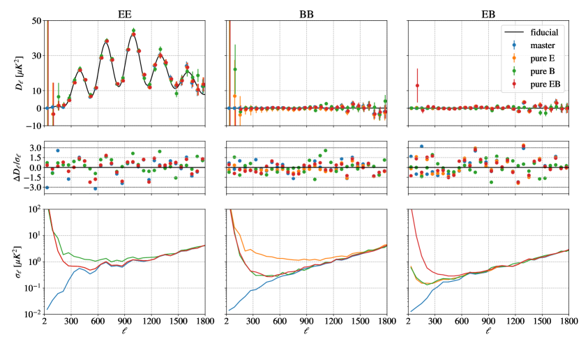
Figure 9: Top: EE (left), BB (center) and EB (right) CMB power spectra for the four purification cases and for 100 Planck-like simulations. The black line represents the fiducial, while the colored points are the simulation average spectra. The error bars represent the error of the mean. Center: EE, BB and EB difference between the simulation average and the fiducial spectra, divided by the error of the mean. Bottom: EE, BB and EB errors of the mean.

The spectra are validated for all the four cases. The error on the spectra is similar for high multipoles, while it is smaller for the master case at low multipoles. Thus, for the analysis conditions considered in this work, the purification process increases the uncertainty of the estimated spectra and turns out to be not useful.

Appendix B Effective beam calculation

Strictly speaking, both CMB data and simulations contain a non-Gaussian beam and a non-ideal pixel window function (see Figure F.1. of [60]). Thus, we employ an effective “smoothing function” $b_{\ell,eff}^{2}$ obtained by taking these steps:

1. From 999 signal-only Planck PR3 simulated $a_{\ell m}^{i}$, not smoothed, we compute the corresponding $C_{\ell}^{i}$ for each simulation $i$.

2. From 999 signal-only Planck PR3 simulated maps at $N_{side}=2048$, that are smoothed with a realistic beam, get the corresponding $C_{\ell,sm}^{i}$ in full sky for each simulation $i$.

3. Divide the two power spectra to obtain $\left(b_{\ell,eff}^{2}\right)^{i}=C_{\ell,sm}^{i}/C_{\ell}^{i}$ for each simulation $i$.

4. Average the smoothing function over the simulation index $i$.

The smoothing function obtained contains both an effective beam window function and an effective pixel window function. This procedure is followed for the PR3 simulations of the 4 component separation methods maps separately, obtaining 4 different effective smoothing functions for Commander, NILC, SEVEM and SMICA. For NPIPE Commander and SEVEM maps we use the same smoothing function computed for PR3. For each component separation method, the same smoothing function is used for each patch.

Appendix C CB auto- and cross-correlation results on simulations

We report in Fig. 10 the auto-correlation of the CB angle maps and their cross-correlation with CMB temperature and polarization fields obtained on simulations. All the spectra are given in terms of bandpowers, as in Sec. 4. Figure 10 shows that the systematic effects included in the simulations have a negligible impact because all the spectra are well compatible with zero, as the deviations from zero are less than $3\sigma$ for all the multipoles considered. As for the data spectra, the scatter around zero of the simulation NPIPE $\alpha\alpha$ spectra and the errors are lower with respect to the PR3 $\alpha\alpha$ case. This is again due to the lower levels of noise present in the NPIPE maps.

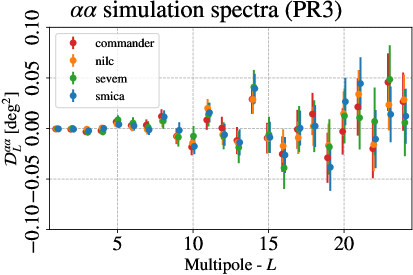
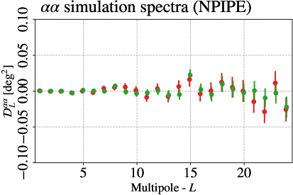
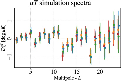
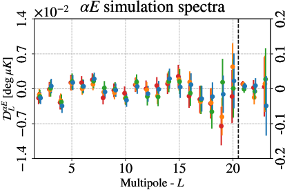
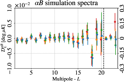
Figure 10: Auto-correlation spectra of the simulation CB angle maps and their cross-correlation with CMB. The dots represent the average of the simulation spectra, while the errors are the errors of the average. The vertical dashed lines highlight a change in the vertical axis range. Top left panel: PR3 $\alpha\alpha$. Top right panel: NPIPE $\alpha\alpha$. Central panel: PR3 $\alpha T$. Bottom left panel: PR3 $\alpha E$. Bottom right panel: PR3 $\alpha B$.

Appendix D Analysis robustness tests

In order to test the robustness of our results, we modify some analysis settings of our pipeline. Since we find good stability for all the considered spectra, for the sake of brevity we present here robustness tests only for the cross-correlation between the CB and the CMB temperature field. This choice is mainly due to the fact that, even if statistically well compatible, the most likely value for $A^{\alpha T}$ is found here negative while in [21] it is positive. Since the analysis in [21] was performed at HEALPix resolution $N_{side}=4$ (while our analysis is performed at $N_{side}=8$) we rerun our codes at lower resolution for the Commander component separation method. The maximum multipole for the $\alpha T$ spectra at this resolution is 12. We find that data and simulations spectra are compatible with zero, as at $N_{side}=8$. However, the scale-invariant amplitude moves towards positive values, as we obtain $\mathrm{A^{\alpha T}=(0.192\pm 1.102)\ \mu K\ deg}$. The constraint is worse than the one at $N_{side}=8$ due to the lower resolution of the patch maps. In addition, if we use a more aggressive mask by extending our mask by the size of one patch as done in [21] ($\approx 15^{\circ}$ at $N_{side}=4$), we obtain $\mathrm{A^{\alpha T}=(1.890\pm 1.297)\ \mu K\ deg}$. Our constraints at $N_{side}=4$ are well compatible (even for the sign of the most likely value) with [21] and with null cross-correlation between the CB and the CMB temperature fields. To test if the change in resolution can explain the shift of the data spectra to more negative values, we calculate the difference between the two data spectra for the first 12 multipoles at the two different resolutions and we compare it with the same quantity calculated on simulations. We find that the shift in the bandpowers is compatible with the scatter of the simulations.

In order to see if the negative sign of the $\mathrm{A^{\alpha T}}$ parameter is given by a bias in the simulations, we subtract the average of the CB simulation maps from all the CB simulations and data maps. We then run the QML estimator for the $D_{L}^{\alpha T}$ spectra and fit with a scale-invariant spectrum for the $\mathrm{A^{\alpha T}}$ parameter. The posteriors move towards slightly less negative values of $\mathrm{A^{\alpha T}}$ and the errors are slightly lower, but this shift cannot explain the change in sign of $\mathrm{A^{\alpha T}}$. The constraints in the debias case are reported in Tab. 5.

case	Commander	NILC	SEVEM	SMICA
reference	$-1.827\pm 0.953$	$-1.229\pm 0.873$	$-2.037\pm 1.038$	$-1.916\pm 0.945$
debias	$-1.766\pm 0.948$	$-1.192\pm 0.868$	$-1.997\pm 1.034$	$-1.886\pm 0.941$
extended	$-1.383\pm 1.098$	$-0.724\pm 0.993$	$-1.636\pm 1.164$	$-1.354\pm 1.066$
$\ell_{min}=302$	$-1.931\pm 0.995$	$-1.439\pm 0.899$	$-2.468\pm 1.092$	$-2.122\pm 0.987$

Table 5: Constraints on the scale invariant power spectrum $A^{\alpha T}$, given in $\mu K\ deg$. The reference case is discussed in Sec. 3. The debias, extended and $\ell_{min}=302$ cases are explained in this Appendix.

To study the effect of possible foregrounds not excluded by the mask applied to the CB angle and CMB temperature maps, we try to use a more aggressive mask. We thus extend the mask shown in the left panel of Fig. 3 by the size of one patch, i.e. $\approx 8^{\circ}$, leaving $\approx$ 60% of the sky non-masked. The scatter of the data spectra around zero is slightly larger than for the non extended mask due to the lower sky fraction, but the compatibility with the null effect is still obtained. The posteriors move towards less negative values of the scale invariant spectrum, but the errors on the parameter increase, again due to the reduced sky fraction. The constraints with the extended mask are reported in Tab. 5.

Finally, we change the CMB multipole range used for the minimization of the $\chi^{2}$ to obtain the CB angles in each patch. We increase the minimum multipole considered from 62 to 302 and then produce the CB angle maps and get the final results. The posteriors move towards more negative values of $\mathrm{A^{\alpha T}}$, but the errors on this parameter increase and there is again good compatibility with null cross-correlation between CB and CMB temperature fields. The constraints with $\ell_{min}=302$ case are reported in Tab. 5.

Appendix E $\alpha\alpha$ and $\alpha T$ joint constraints

We set 2D constraints on $A^{\alpha\alpha}$ and $A^{\alpha T}$ following the methodology explained in [21]. We report in Fig. 11 the validation of the 2D analysis for the SMICA case. The posterior shown in Fig. 11 is the product of the posteriors obtained from the single simulations. Since the simulations do not contain the CB effect and the posterior is consistent with zero, the analysis is validated. We obtain similar results for the other component separation methods.

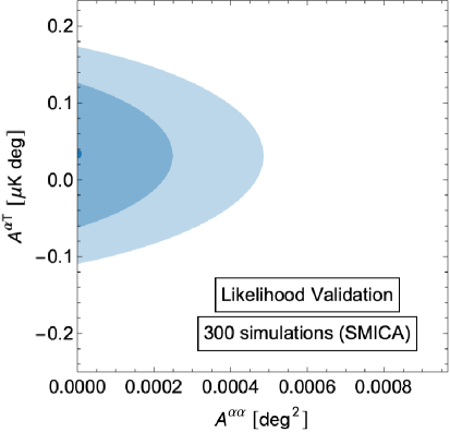
Figure 11: 2D contour plots for the $\mathrm{A^{\alpha\alpha}}$ and $\mathrm{A^{\alpha T}}$ parameters obtained with the SMICA simulations. The darker (lighter) area represents the 68% (95%) confidence region.

In Figure 12 we show the 2D contour plots for the $\mathrm{A^{\alpha\alpha}}$ and $\mathrm{A^{\alpha T}}$ parameters obtained with the Commander, NILC, SEVEM and SMICA CB data maps for the PR3 case and with the Commander CMB temperature map. We use two different masks for the CB angles and CMB temperature maps in order to exploit the largest amount of data: the former has a sky fraction of 74%, while the latter of 84%. The covariance matrices are built analytically. For this motivation, the uncertainties in the 2D case are larger with respect to the 1D analysis described in Sec. 3, as in the latter the CB cosmic variance is not taken into account. The four component separation methods provide similar constraints. The SEVEM component separation method is the one having the lowest compatibility with null CB. However, the deviation is not larger than 3 standard deviations. Thus, we find no evidence for the CB effect.

We then marginalize the 2D posterior distribution functions over $\mathrm{A^{\alpha T}}$, obtaining the posterior distribution functions of $\mathrm{A^{\alpha\alpha}}$ reported in Fig. 13 (solid curves). We also slice the 2D probability at $\mathrm{A^{\alpha T}}=0$, obtaining the probability distribution of $\mathrm{A^{\alpha\alpha}}$ shown in Fig. 13 (dashed curves). The posterior is closer to zero for the sliced case, providing more stringent constraints than the marginalized posterior. The four component separation methods agree among themselves, even if the SEVEM distribution is larger than the other three, reflecting what discussed for Fig. 12.

If we instead marginalize over $\mathrm{A^{\alpha\alpha}}$, we obtain the posterior distribution functions for $\mathrm{A^{\alpha T}}$ reported in Fig. 14 (solid curves). Slicing the 2D contours at $\mathrm{A^{\alpha\alpha}}=0$, we obtain the probability distribution of $\mathrm{A^{\alpha T}}$ shown in Fig. 14 (dashed curves). Also here the sliced case provides tighter posteriors than for the marginalized one, as expected. All these results are compatible with null CB.

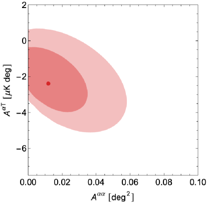
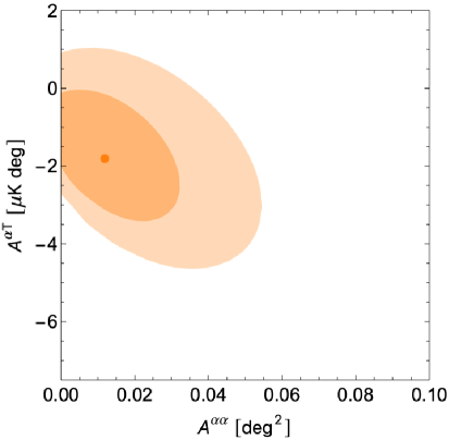
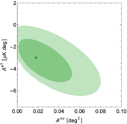
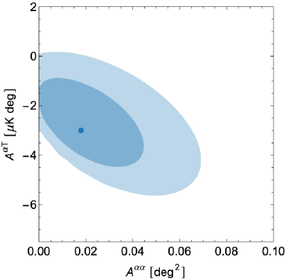
Figure 12: 2-dimensional contour plots for the $\mathrm{A^{\alpha\alpha}}$ and $\mathrm{A^{\alpha T}}$ parameters obtained with the Commander (top left panel), NILC (top right panel), SEVEM (bottom left panel) and SMICA (bottom right panel) data. The darker (lighter) area represents the 68% (95%) confidence region.

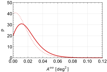
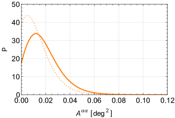
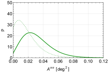
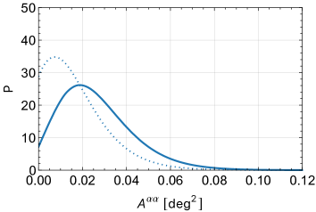
Figure 13: Posterior distribution functions for the $\mathrm{A^{\alpha\alpha}}$ parameter obtained from Commander (top left panel), NILC (top right panel), SEVEM (bottom left panel) and SMICA (bottom right panel) data. The solid curves are computed marginalising the 2D distribution functions over $\mathrm{A^{\alpha T}}$ and the dashed ones slicing the 2D distribution functions at $\mathrm{A^{\alpha T}}=0$.

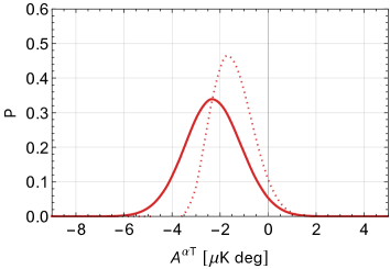
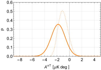
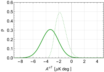
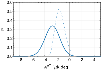
Figure 14: Posterior distribution functions for the $\mathrm{A^{\alpha T}}$ parameter obtained from Commander (top left panel), NILC (top right panel), SEVEM (bottom left panel) and SMICA (bottom right panel) data. The solid curves are computed marginalising the 2D distribution functions over $\mathrm{A^{\alpha\alpha}}$ and the dashed ones slicing the 2D distribution functions at $\mathrm{A^{\alpha\alpha}}=0$.

References

- [1] C.S. Wu, E. Ambler, R.W. Hayward, D.D. Hoppes and R.P. Hudson, Experimental Test of Parity Conservation in Decay, Phys. Rev. 105 (1957) 1413.
- [2] S.M. Carroll, G.B. Field and R. Jackiw, Limits on a Lorentz and Parity Violating Modification of Electrodynamics, Phys. Rev. D 41 (1990) 1231.
- [3] S.M. Carroll and G.B. Field, The Einstein equivalence principle and the polarization of radio galaxies, Phys. Rev. D 43 (1991) 3789.
- [4] V.A. Kostelecky and M. Mewes, Lorentz-violating electrodynamics and the cosmic microwave background, Phys. Rev. Lett. 99 (2007) 011601 [astro-ph/0702379].
- [5] V.A. Kostelecky and N. Russell, Data Tables for Lorentz and CPT Violation, 0801.0287.
- [6] Planck Collaboration Int. XLIX, Planck intermediate results. XLIX. Parity-violation constraints from polarization data, A&A 596 (2016) A110 [1605.08633].
- [7] A. Lue, L.-M. Wang and M. Kamionkowski, Cosmological signature of new parity violating interactions, Phys. Rev. Lett. 83 (1999) 1506 [astro-ph/9812088].
- [8] B. Feng, M. Li, J.-Q. Xia, X. Chen and X. Zhang, Searching for CPT Violation with Cosmic Microwave Background Data from WMAP and BOOMERANG, Phys. Rev. Lett. 96 (2006) 221302 [astro-ph/0601095].
- [9] J.-Q. Xia, H. Li, X.-l. Wang and X.-m. Zhang, Testing CPT Symmetry with CMB Measurements, Astron. Astrophys. 483 (2008) 715 [0710.3325].
- [10] F. Finelli and M. Galaverni, Rotation of Linear Polarization Plane and Circular Polarization from Cosmological Pseudo-Scalar Fields, Phys. Rev. D 79 (2009) 063002 [0802.4210].
- [11] M. Li and X. Zhang, Cosmological CPT violating effect on CMB polarization, Phys. Rev. D 78 (2008) 103516 [0810.0403].
- [12] G. Gubitosi, L. Pagano, G. Amelino-Camelia, A. Melchiorri and A. Cooray, A Constraint on Planck-scale Modifications to Electrodynamics with CMB polarization data, JCAP 08 (2009) 021 [0904.3201].
- [13] L. Pagano, P. de Bernardis, G. De Troia, G. Gubitosi, S. Masi, A. Melchiorri et al., CMB Polarization Systematics, Cosmological Birefringence and the Gravitational Waves Background, Phys. Rev. D 80 (2009) 043522 [0905.1651].
- [14] G. Gubitosi and F. Paci, Constraints on cosmological birefringence energy dependence from CMB polarization data, JCAP 02 (2013) 020 [1211.3321].
- [15] G. Gubitosi, M. Martinelli and L. Pagano, Including birefringence into time evolution of CMB: current and future constraints, JCAP 12 (2014) 020 [1410.1799].
- [16] A. Gruppuso, G. Maggio, D. Molinari and P. Natoli, A note on the birefringence angle estimation in CMB data analysis, JCAP 05 (2016) 020 [1604.05202].
- [17] M. Kamionkowski, How to De-Rotate the Cosmic Microwave Background Polarization, Phys. Rev. Lett. 102 (2009) 111302 [0810.1286].
- [18] V. Gluscevic, M. Kamionkowski and A. Cooray, De-Rotation of the Cosmic Microwave Background Polarization: Full-Sky Formalism, Phys. Rev. D 80 (2009) 023510 [0905.1687].
- [19] G. Gubitosi, M. Migliaccio, L. Pagano, G. Amelino-Camelia, A. Melchiorri, P. Natoli et al., Using CMB data to constrain non-isotropic Planck-scale modifications to Electrodynamics, JCAP 11 (2011) 003 [1106.6049].
- [20] V. Gluscevic, D. Hanson, M. Kamionkowski and C.M. Hirata, First CMB Constraints on Direction-Dependent Cosmological Birefringence from WMAP-7, Phys. Rev. D 86 (2012) 103529 [1206.5546].
- [21] A. Gruppuso, D. Molinari, P. Natoli and L. Pagano, Planck 2018 constraints on anisotropic birefringence and its cross-correlation with CMB anisotropy, JCAP 11 (2020) 066 [2008.10334].
- [22] J.R. Eskilt, Frequency-Dependent Constraints on Cosmic Birefringence from the LFI and HFI Planck Data Release 4, 2201.13347.
- [23] Y. Minami and E. Komatsu, New extraction of the cosmic birefringence from the planck 2018 polarization data, Phys. Rev. Lett. 125 (2020) 221301.
- [24] P. Diego-Palazuelos et al., Cosmic Birefringence from the Planck Data Release 4, Phys. Rev. Lett. 128 (2022) 091302 [2201.07682].
- [25] E. Komatsu, New physics from polarised light of the cosmic microwave background, 2202.13919.
- [26] J.R. Eskilt and E. Komatsu, Improved Constraints on Cosmic Birefringence from the WMAP and Planck Cosmic Microwave Background Polarization Data, 2205.13962.
- [27] A. Abghari, R.M. Sullivan, L.T. Hergt and D. Scott, Constraints on cosmic birefringence using -mode polarisation, 2203.10733.
- [28] D. Contreras, P. Boubel and D. Scott, Constraints on direction-dependent cosmic birefringence from Planck polarization data, JCAP 12 (2017) 046 [1705.06387].
- [29] T. Namikawa et al., Atacama Cosmology Telescope: Constraints on cosmic birefringence, Phys. Rev. D 101 (2020) 083527 [2001.10465].
- [30] SPT collaboration, Searching for Anisotropic Cosmic Birefringence with Polarization Data from SPTpol, Phys. Rev. D 102 (2020) 083504 [2006.08061].
- [31] W. Zhao and M. Li, Fluctuations of cosmological birefringence and the effect on cmb -mode polarization, Phys. Rev. D 89 (2014) 103518.
- [32] A. Greco, N. Bartolo and A. Gruppuso, Cosmic Birefringence: Cross-Spectra and Cross-Bispectra with CMB Anisotropies, 2202.04584.
- [33] T. Karwal and M. Kamionkowski, Dark energy at early times, the Hubble parameter, and the string axiverse, Phys. Rev. D 94 (2016) 103523 [1608.01309].
- [34] V. Poulin, T.L. Smith, T. Karwal and M. Kamionkowski, Early Dark Energy Can Resolve The Hubble Tension, Phys. Rev. Lett. 122 (2019) 221301 [1811.04083].
- [35] N. Schöneberg, G. Franco Abellán, A. Pérez Sánchez, S.J. Witte, V. Poulin and J. Lesgourgues, The Olympics: A fair ranking of proposed models, 2107.10291.
- [36] L.M. Capparelli, R.R. Caldwell and A. Melchiorri, Cosmic birefringence test of the Hubble tension, Phys. Rev. D 101 (2020) 123529 [1909.04621].
- [37] Planck Collaboration I, Planck 2018 results. I. Overview, and the cosmological legacy of Planck, A&A 641 (2020) A1 [1807.06205].
- [38] Planck Collaboration Int. LVII, Planck intermediate results. LVII. NPIPE: Joint Planck LFI and HFI data processing, A&A 643 (2020) 42 [2007.04997].
- [39] Planck Collaboration IV, Planck 2018 results. IV. Diffuse component separation, A&A 641 (2020) A4 [1807.06208].
- [40] K.M. Górski, E. Hivon, A.J. Banday, B.D. Wandelt, F.K. Hansen, M. Reinecke et al., HEALPix - A Framework for high resolution discretization, and fast analysis of data distributed on the sphere, Astrophys. J. 622 (2005) 759 [astro-ph/0409513].
- [41] Planck Collaboration XII, Planck 2015 results. XII. Full Focal Plane simulations, A&A 594 (2016) A12 [1509.06348].
- [42] Planck Collaboration III, Planck 2018 results. III. High Frequency Instrument data processing, A&A 641 (2020) A3 [1807.06207].
- [43] LSST Dark Energy Science collaboration, A unified pseudo- framework, Mon. Not. Roy. Astron. Soc. 484 (2019) 4127 [1809.09603].
- [44] Planck Collaboration II, Planck 2018 results. II. Low Frequency Instrument data processing, A&A 641 (2020) A2 [1807.06206].
- [45] J. Grain, M. Tristram and R. Stompor, Polarized CMB spectrum estimation using the pure pseudo cross-spectrum approach, Phys. Rev. D 79 (2009) 123515 [0903.2350].
- [46] E. Hivon, K.M. Gorski, C.B. Netterfield, B.P. Crill, S. Prunet and F. Hansen, Master of the cosmic microwave background anisotropy power spectrum: a fast method for statistical analysis of large and complex cosmic microwave background data sets, Astrophys. J. 567 (2002) 2 [astro-ph/0105302].
- [47] M. Tegmark and A. de Oliveira-Costa, How to measure CMB polarization power spectra without losing information, Phys. Rev. D 64 (2001) 063001 [astro-ph/0012120].
- [48] A. Gruppuso, A. De Rosa, P. Cabella, F. Paci, F. Finelli, P. Natoli et al., New estimates of the CMB angular power spectra from the WMAP 5 yrs low resolution data, Mon. Not. Roy. Astron. Soc. 400 (2009) 463 [0904.0789].
- [49] S. Vanneste, S. Henrot-Versillé, T. Louis and M. Tristram, Quadratic estimator for CMB cross-correlation, Phys. Rev. D 98 (2018) 103526 [1807.02484].
- [50] L. Pagano, J.M. Delouis, S. Mottet, J.L. Puget and L. Vibert, Reionization optical depth determination from Planck HFI data with ten percent accuracy, Astron. Astrophys. 635 (2020) A99 [1908.09856].
- [51] Planck Collaboration XI, Planck 2015 results. XI. CMB power spectra, likelihoods, and robustness of parameters, A&A 594 (2016) A11 [1507.02704].
- [52] Planck Collaboration V, Planck 2018 results. V. Power spectra and likelihoods, A&A 641 (2020) A5 [1907.12875].
- [53] Planck Collaboration ES, The Legacy Explanatory Supplement, https://www.cosmos.esa.int/web/planck/pla, ESA (2018).
- [54] K. Benabed, J.F. Cardoso, S. Prunet and E. Hivon, TEASING: a fast and accurate approximation for the low multipole likelihood of the Cosmic Microwave Background temperature, Mon. Not. Roy. Astron. Soc. 400 (2009) 219 [0901.4537].
- [55] Planck Collaboration VIII, Planck 2013 results. VIII. HFI photometric calibration and mapmaking, A&A 571 (2014) A8 [1303.5069].
- [56] C. Rosset, M. Tristram, N. Ponthieu, P. Ade, J. Aumont, A. Catalano et al., Planck pre-launch status: High Frequency Instrument polarization calibration, A&A 520 (2010) A13 [1004.2595].
- [57] A. Zonca, L. Singer, D. Lenz, M. Reinecke, C. Rosset, E. Hivon et al., healpy: equal area pixelization and spherical harmonics transforms for data on the sphere in Python, Journal of Open Source Software 4 (2019) 1298.
- [58] C.R. Harris et al., Array programming with NumPy, Nature 585 (2020) 357 [2006.10256].
- [59] J.D. Hunter, Matplotlib: A 2D Graphics Environment, Comput. Sci. Eng. 9 (2007) 90.
- [60] Planck Collaboration VII, Planck 2013 results. VII. HFI time response and beams, A&A 571 (2014) A7 [1303.5068].