Computational Mean-field Games on Manifolds

Jiajia Yu111J. Yu and R. Lai’s work are supported in part by an NSF Career Award DMS–1752934 and NSF DMS-2134168. yuj12@rpi.edu Rongjie Lai222J. Yu and R. Lai’s work are supported in part by an NSF Career Award DMS–1752934 and NSF DMS-2134168. lair@rpi.edu Wuchen Li333W. Li’s work is supported in part by AFOSR MURI FP 9550-18-1-502 and NSF RTG: 2038080. wuchen@mailbox.sc.edu Stanley Osher444S. Osher’s work is supported in part by AFOSR MURI FP 9550-18-1-502, and ONR grants: N00014-20-1-2093, and N00014-20-1-2787. sjo@math.ucla.edu
Abstract

Conventional Mean-field games/control study the behavior of a large number of rational agents moving in the Euclidean spaces. In this work, we explore the mean-field games on Riemannian manifolds. We formulate the mean-field game Nash Equilibrium on manifolds. We also establish the equivalence between the PDE system and the optimality conditions of the associated variational form on manifolds. Based on triangular mesh representation of two-dimensional manifolds, we design a proximal gradient method for variational mean-field games. Our comprehensive numerical experiments on various manifolds illustrate the effectiveness and flexibility of the proposed model and numerical methods.

keywords:
Mean-field games , Manifolds , Proximal gradient method
MSC:
[2020] 49M41 , 49M25 , 53Z99
journal:
\affiliation

[1]organization=Department of Mathematics, Rensselaer Polytechnic Institute, city=Troy, postcode=NY 12180, country=USA \affiliation[2]organization=Department of Mathematics, University of South Carolina, city=Columbia, postcode=SC 29208, country=USA \affiliation[3]organization=Department of Mathematics, University of California, Los Angeles, city=Los Angeles, postcode=CA 90095, country=USA

1 Introduction

Mean-field games (MFG) [27, 28, 31] study the behavior of a large number of rational agents in an non-cooperative game. It has wide applications in various fields, such as economics [1, 23], engineering [18, 50] as well as machine learning and reinforcement learning [16, 49, 51, 19]. Recently, mean field control problems have been extended into chemistry, biology , pandemic control, traffic flow models and social dynamics [35, 36, 37, 38, 22]. An important task in mean-field games is to study the flow of all the agents in the state space and to understand behavior of mean-field Nash equilibrium.

Conventional studies of MFG focus on choice of the state space as a Euclidean flat domain, for instance, [0,1]dsuperscript01𝑑[0,1]^{d} with periodic boundary conditions. Besides research on Euclidean flat domains, there are existing work focusing MFGs on graphs [21] or graphon state spaces  [24, 26, 12]. However, such spaces may not be adequate to reflect the metric structure of state spaces in many applications. For instance, the problems of population flows or resource distributions on the Earth are actually defined on a sphere. In machine learning, the manifold hypothesis is commonly used [17, 20], since many real world data sets are actually samples from low-dimensional manifolds in a high dimensional ambient space. Therefore, it is quite natural and necessary to explore mean-field game/control problems on manifolds. In this work, we would like to generalize the concepts of finite horizon mean-field games and mean-field Nash Equilibrium from Euclidean spaces to manifolds, and propose a numerical method to compute the Nash Equilibrium.

In this study, we consider a game with infinitely many indistinguishable agents on a compact and smooth manifold \mathcal{M} within the time interval [0,1]01[0,1]. At any time t[0,1]𝑡01t\in[0,1], each agent is in a certain state 𝐱𝐱\mathbf{x}\in\mathcal{M} and the state of all agents forms a distribution ρ(,t)𝒫()𝜌𝑡𝒫\rho(\cdot,t)\in\mathcal{P}(\mathcal{M}). For each agent at t𝑡t, given its current state 𝐱𝐱\mathbf{x} and the anticipation of future state distribution ρ(,s),s[t,1]𝜌𝑠𝑠𝑡1\rho(\cdot,s),s\in[t,1], the game is to optimize a control 𝐯(𝐱(s),s)𝐯𝐱𝑠𝑠\mathbf{v}(\mathbf{x}(s),s) to guide its future trajectory 𝐱(s),s(t,1]𝐱𝑠𝑠𝑡1\mathbf{x}(s),s\in(t,1] in order to minimize a cost Jρ(𝐱,t,𝐯)superscript𝐽𝜌𝐱𝑡𝐯J^{\rho}(\mathbf{x},t,\mathbf{v}). Therefore the optimal control 𝐯𝐯\mathbf{v} depends on the state distribution ρ𝜌\rho. Although the state change of any single agent does not change ρ(,t)𝜌𝑡\rho(\cdot,t), when all the agents take the same control, the state distribution ρ𝜌\rho changes accordingly. Thus the optimal control 𝐯𝐯\mathbf{v} and the state distribution ρ𝜌\rho are interdependent, and the Nash Equilibrium [44, 14], the special pair of (𝐯,ρ)𝐯𝜌(\mathbf{v},\rho), is an especially interesting topic in mean-field game.

In the conventional Euclidean setup, it has been shown that the mean-field Nash Equilibrium is the solution of a forward-backward PDE system [31, 28, 27]. We generalize this result to MFG on manifolds. Meanwhile, for a potential mean-field game on a Euclidean domain  [31, 13, 9, 10], its optimality condition is exactly the forward-backward PDE system under mild conditions. Thus, the Nash Equilibrium can be obtained by searching for the stationary point of the optimization problem. In this work, we show that the equivalence between the PDE formulation and variational formulation of mean-field game still holds on manifolds. It is worth mentioning that [48] studies dynamic optimal transport, a special form of potential mean-field games, on manifolds. In this work, we consider more general forms of mean-field games on manifolds and we are interested in both the PDE and variational formulations.

There are different approaches to numerically solve mean-field games on Euclidean domains, such as finite difference methods [3, 2], monotone flows [5, 25], optimization algorithms [8, 11, 52] and neural networks [15, 39, 47]. We refer readers to the surveys [4, 32] for more details of the numerical methods on Euclidean domains. In our manifold setting, we focus on the variational formulation to numerically compute the Nash Equilibrium. With the help of triangular mesh and computational geometry strategies [43], we approximate the manifold, probability space and vector field space and formulate the discrete optimization problem. Once the discretization is provided, most of existing optimization-based algorithms can be adapted to solve the proposed discretization problem. In this work, we specifically use an optimization-based algorithm proposed in [52] since it is flexible and efficient. This algorithm is adapted from the proximal gradient descent method considered in [46, 6, 7].

Contributions: We summarize our contributions as follows:

  1. (i)

    We generalize the concept of mean-field games to manifolds and derive the corresponding geometric PDE formulation of the Nash Equilibrium.

  2. (ii)

    We show the equivalence of the PDE formulation and variational formulation of mean-field games on manifolds.

  3. (iii)

    We propose a numerical method for solving the variational problem based on a proximal gradient descent method. Comprehensive experiments demonstrate the effectiveness of the proposed method.

Organization: Our paper is organized as follows. In section 2, we derive the PDE formulation of mean-field Nash Equilibrium on manifolds. We also show that the PDE system is actually the optimality condition of an optimization problem, the potential mean-field game, on the manifold. We discretize the potential MFG problems in space and time domain in section 3, and adapt a proximal gradient method to solve the discrete counterparts in section 4. In section 5, we provide numerical experiments that solve potential mean-field games with local or non-local interaction costs on different manifolds.

2 Mean-field games on manifolds

In this section, we generalize the concepts of finite horizon mean-field games (MFGs) and their variational forms from conventional Euclidean domains to smooth and compact Riemannian manifolds.

2.1 Mean-field games on manifold

Let’s begin with some notations for convenience. We consider MFG on (,g)𝑔(\mathcal{M},g), a d𝑑d-dimensional smooth compact manifold with a Riemannian metric g𝑔g. As a natural extension of MFG on Euclidean domains, controls at the state 𝐱𝐱\mathbf{x}\in\mathcal{M} are defined as elements in T𝐱subscriptT𝐱\mathrm{T}_{\mathbf{x}}\mathcal{M}, the tangent space of \mathcal{M} at 𝐱𝐱\mathbf{x}\in\mathcal{M}. We further denote T={(𝐱,𝐩)|𝐩T𝐱}Tconditional-set𝐱𝐩𝐩subscriptT𝐱\mathrm{T}\mathcal{M}=\{(\mathbf{x},\mathbf{p})~{}|~{}\mathbf{p}\in\mathrm{T}_{\mathbf{x}}\mathcal{M}\} for the tangent bundle of \mathcal{M}; use Γ(T)ΓT\Gamma(\mathrm{T}\mathcal{M}) for the set of continuous vector fields on \mathcal{M}; and write 𝒫()𝒫\mathcal{P}(\mathcal{M}) for all probability density on (,g)𝑔(\mathcal{M},g) under the volume measurement induced by the metric g𝑔g.

To derive a first-order MFG system on \mathcal{M}, we consider a finite horizon game on the time interval [0,1]01[0,1] with the state space \mathcal{M}. More specifically, we assume that there is a continuum number of agents, and each agent takes a state 𝐱𝐱\mathbf{x}\in\mathcal{M} at any time t[0,1]𝑡01t\in[0,1]. We write the state density of all the agents along t[0,1]𝑡01t\in[0,1] as ρC([0,1];𝒫())𝜌𝐶01𝒫\rho\in C([0,1];\mathcal{P}(\mathcal{M})); and assume that the impact of any single agent to ρ𝜌\rho is negligible. Since all the agents have the same goal in a mean-field game, it is sufficient to take a representative agent as an example. Suppose that an agent is in state 𝐱𝐱\mathbf{x} at time t𝑡t, the agent aims at choosing a control 𝐯C((t,1];Γ(T))𝐯𝐶𝑡1ΓT\mathbf{v}\in C((t,1];\Gamma(\mathrm{T}\mathcal{M})) to guide the trajectory

d𝐱(t)=𝐯(𝐱,t)dt.d𝐱𝑡𝐯𝐱𝑡d𝑡\mathrm{d}\mathbf{x}(t)=\mathbf{v}(\mathbf{x},t)\mathrm{d}t. (1)

in order to minimize the cost

Jρ(𝐱,t,𝐯):=t1[L(𝐱(s),𝐯(𝐱(s),s)+F(𝐱(s),ρ(,s))]ds+FT(𝐱(1),ρ(,1)).J^{\rho}(\mathbf{x},t,\mathbf{v}):=\int_{t}^{1}\left[L(\mathbf{x}(s),\mathbf{v}(\mathbf{x}(s),s)+F(\mathbf{x}(s),\rho(\cdot,s))\right]\mathrm{d}s+F_{T}(\mathbf{x}(1),\rho(\cdot,1)). (2)

Here L:T[0,+):𝐿T0L:\mathrm{T}\mathcal{M}\to[0,+\infty) is the dynamic cost, F:×𝒫()[0,+):𝐹𝒫0F:\mathcal{M}\times\mathcal{P}(\mathcal{M})\to[0,+\infty) is the interaction cost, ρ(,s)𝒫()𝜌𝑠𝒫\rho(\cdot,s)\in\mathcal{P}(\mathcal{M}) is the density of all agents at time s𝑠s, and FT:×𝒫()[0,+):subscript𝐹𝑇𝒫0F_{T}:\mathcal{M}\times\mathcal{P}(\mathcal{M})\to[0,+\infty) is the terminal cost. Note that the control 𝐯𝐯\mathbf{v} and the state distribution ρ𝜌\rho are involved interactively. The optimal control 𝐯ρ:=argmin𝐯Jρ(𝐱,t,𝐯)assignsuperscript𝐯𝜌subscriptargmin𝐯superscript𝐽𝜌𝐱𝑡𝐯\mathbf{v}^{\rho}:=\operatorname*{argmin}_{\mathbf{v}}J^{\rho}(\mathbf{x},t,\mathbf{v}) generally depends on the evolution of the state distribution ρ𝜌\rho. Meanwhile, with given initial distribution ρ(,0):=ρ0𝒫()assign𝜌0subscript𝜌0𝒫\rho(\cdot,0):=\rho_{0}\in\mathcal{P}(\mathcal{M}), the distribution of agents ρ𝜌\rho is determined by the control 𝐯C([0,1];Γ(T))𝐯𝐶01ΓT\mathbf{v}\in C([0,1];\Gamma(\mathrm{T}\mathcal{M})) through equation (1). The mean-field game problem is especially interested in a special pair of them, the Nash Equilibrium, which is the same as the conventional Euclidean case [44, 14],

Definition 2.1 (Nash Equilibrium).

A pair of control and state distribution (𝐯,ρ)𝐯𝜌(\mathbf{v},\rho) is called a Nash Equilibrium if the following two conditions hold,

  1. 1.

    (Optimality) For any t[0,1],𝐱formulae-sequence𝑡01𝐱t\in[0,1],\mathbf{x}\in\mathcal{M}, Jρ(𝐱,t,𝐯)Jρ(𝐱,t,𝐮),𝐮C([0,1];Γ(T))formulae-sequencesuperscript𝐽𝜌𝐱𝑡𝐯superscript𝐽𝜌𝐱𝑡𝐮for-all𝐮𝐶01ΓTJ^{\rho}(\mathbf{x},t,\mathbf{v})\leq J^{\rho}(\mathbf{x},t,\mathbf{u}),~{}\forall~{}\mathbf{u}\in C([0,1];\Gamma(\mathrm{T}\mathcal{M})).

  2. 2.

    (Consistency) ρ(,0)=ρ0𝜌0subscript𝜌0\rho(\cdot,0)=\rho_{0} where ρ0subscript𝜌0\rho_{0} is the state distribution of all the agents at t=0𝑡0t=0. And ρ(,t)𝜌𝑡\rho(\cdot,t) is the state distribution of all the agents at time t𝑡t following the control 𝐯𝐯\mathbf{v}.

With the definition, if (𝐯,ρ)𝐯𝜌(\mathbf{v},\rho) is a Nash Equilibrium of a MFG on (,g)𝑔(\mathcal{M},g), then the optimality condition ensures that 𝐯𝐯\mathbf{v} is the optimal control for given state distribution ρ𝜌\rho, and the consistency requires that 𝐯𝐯\mathbf{v} lead to the state distribution ρ𝜌\rho.

According to [31, 28], in Euclidean space, a Nash Equilibrium can be described by a PDE system, which includes a backward Hamiltonian-Jacobi-Bellman (HJB) equation by the optimality condition and a forward continuity equation by the consistency condition. In the rest, we will establish a similar PDE description of a Nash Equilibirum on manifolds.

Similar as the Euclidean case [31, 28], let the value function ϕitalic-ϕ\phi be the cost with the optimal control,

ϕρ(𝐱,t):=inf𝐯C([0,1];Γ(T))Jρ(𝐱,t,𝐯).assignsuperscriptitalic-ϕ𝜌𝐱𝑡subscriptinfimum𝐯𝐶01ΓTsuperscript𝐽𝜌𝐱𝑡𝐯\phi^{\rho}(\mathbf{x},t):=\inf_{\mathbf{v}\in C([0,1];\Gamma(\mathrm{T}\mathcal{M}))}J^{\rho}(\mathbf{x},t,\mathbf{v}). (3)

and H𝐻H be the manifold Hamiltonian defined on the tangent bundle of \mathcal{M} [34]

H:T,H(𝐱,𝐪):=sup𝐩T𝐱{𝐪,𝐩g(𝐱)L(𝐱,𝐩)}.:𝐻formulae-sequenceTassign𝐻𝐱𝐪subscriptsupremum𝐩subscriptT𝐱subscript𝐪𝐩𝑔𝐱𝐿𝐱𝐩H:\mathrm{T}\mathcal{M}\to\mathbb{R},\quad H(\mathbf{x},\mathbf{q}):=\sup_{\mathbf{p}\in\mathrm{T}_{\mathbf{x}}\mathcal{M}}\left\{-\langle\mathbf{q},\mathbf{p}\rangle_{g(\mathbf{x})}-L(\mathbf{x},\mathbf{p})\right\}. (4)

we have the following theorem.

Theorem 2.2.

If (𝐯,ρ)𝐯𝜌(\mathbf{v},\rho) is a Nash Equilibrium of the aforementioned mean-field game on (,g)𝑔(\mathcal{M},g), then

𝐯(𝐱,t)=argmin𝐩T𝐱{L(𝐱,𝐩)+ϕ(𝐱,t),𝐩g(𝐱)}=𝐪H(𝐱,ϕ(𝐱,t)).𝐯𝐱𝑡subscriptargmin𝐩subscriptT𝐱𝐿𝐱𝐩subscriptsubscriptitalic-ϕ𝐱𝑡𝐩𝑔𝐱subscript𝐪𝐻𝐱subscriptitalic-ϕ𝐱𝑡\mathbf{v}(\mathbf{x},t)=\operatorname*{argmin}_{\mathbf{p}\in\mathrm{T}_{\mathbf{x}}\mathcal{M}}\left\{L(\mathbf{x},\mathbf{p})+\langle\nabla_{\mathcal{M}}\phi(\mathbf{x},t),\mathbf{p}\rangle_{g(\mathbf{x})}\right\}=-\partial_{\mathbf{q}}H(\mathbf{x},\nabla_{\mathcal{M}}\phi(\mathbf{x},t)). (5)

and ρ,ϕ𝜌italic-ϕ\rho,\phi solve

{tϕ(𝐱,t)+H(𝐱,ϕ(𝐱,t))=F(𝐱,ρ(,t)),tρ(𝐱,t)(ρ(𝐱,t)𝐪H(𝐱,ϕ(𝐱,t)))=0,ϕ(𝐱,1)=FT(𝐱,ρ(,1)),ρ(,0)=ρ0.\left\{\begin{aligned} &-\partial_{t}\phi(\mathbf{x},t)+H(\mathbf{x},\nabla_{\mathcal{M}}\phi(\mathbf{x},t))=F(\mathbf{x},\rho(\cdot,t)),\\ &\partial_{t}\rho(\mathbf{x},t)-\nabla_{\mathcal{M}}\cdot(\rho(\mathbf{x},t)\partial_{\mathbf{q}}H(\mathbf{x},\nabla_{\mathcal{M}}\phi(\mathbf{x},t)))=0,\\ &\phi(\mathbf{x},1)=F_{T}(\mathbf{x},\rho(\cdot,1)),\qquad\rho(\cdot,0)=\rho_{0}.\end{aligned}\right. (6)

Before proving the theorem, we give several remarks to explain notations.

Remark 2.3.

We emphasis that the metrics ,g(𝐱)subscript𝑔𝐱\langle\cdot,\cdot\rangle_{g(\mathbf{x})}, and operators ,\nabla_{\mathcal{M}},\nabla_{\mathcal{M}}\cdot are based on the manifold metric g𝑔g as a generalization of the conventional equations which only depend on the flat Euclidean metric. More details on differential geometry can be refereed in [33].

As an example, let \mathcal{M} be a two-dimensional manifold embedded in 3superscript3\mathbb{R}^{3} with an induced metric g𝑔g on the manifold. To be precise, consider X:Ξ23,(ξ1,ξ2)X(ξ1,ξ2)X:\Xi\subset\mathbb{R}^{2}\to\mathcal{M}\subset\mathbb{R}^{3},(\xi^{1},\xi^{2})\mapsto X(\xi^{1},\xi^{2}) as a local chart of \mathcal{M}, then for any 𝐱=X(ξ1,ξ2)𝐱𝑋superscript𝜉1superscript𝜉2\mathbf{x}=X(\xi^{1},\xi^{2}) on the chart, the tangent space is T𝐱=span{ξ1X,ξ2X}subscriptT𝐱spansubscriptsuperscript𝜉1𝑋subscriptsuperscript𝜉2𝑋\mathrm{T}_{\mathbf{x}}\mathcal{M}=\operatorname*{span}\{\partial_{\xi^{1}}X,\partial_{\xi^{2}}X\}. The matrix representation of the induced metric g𝑔g in the coordinate chart X𝑋X is provided as:

gX(𝐱):=((ξ1X)ξ1X(ξ1X)ξ2X(ξ2X)ξ1X(ξ2X)ξ2X).assignsubscript𝑔𝑋𝐱matrixsuperscriptsubscriptsuperscript𝜉1𝑋topsubscriptsuperscript𝜉1𝑋superscriptsubscriptsuperscript𝜉1𝑋topsubscriptsuperscript𝜉2𝑋superscriptsubscriptsuperscript𝜉2𝑋topsubscriptsuperscript𝜉1𝑋superscriptsubscriptsuperscript𝜉2𝑋topsubscriptsuperscript𝜉2𝑋g_{X}(\mathbf{x}):=\left(\begin{matrix}(\partial_{\xi^{1}}X)^{\top}\partial_{\xi^{1}}X&(\partial_{\xi^{1}}X)^{\top}\partial_{\xi^{2}}X\\ (\partial_{\xi^{2}}X)^{\top}\partial_{\xi^{1}}X&(\partial_{\xi^{2}}X)^{\top}\partial_{\xi^{2}}X\end{matrix}\right). (7)

Any tangent vectors 𝐩,𝐪T𝐱𝐩𝐪subscriptT𝐱\mathbf{p},\mathbf{q}\in\mathrm{T}_{\mathbf{x}}\mathcal{M} have the corresponding coordinate decomposition 𝐩=pX1ξ1X+pX2ξ2X𝐩superscriptsubscript𝑝𝑋1subscriptsuperscript𝜉1𝑋superscriptsubscript𝑝𝑋2subscriptsuperscript𝜉2𝑋\mathbf{p}=p_{X}^{1}\partial_{\xi^{1}}X+p_{X}^{2}\partial_{\xi^{2}}X, 𝐪=qX1ξ1X+qX2ξ2X𝐪superscriptsubscript𝑞𝑋1subscriptsuperscript𝜉1𝑋superscriptsubscript𝑞𝑋2subscriptsuperscript𝜉2𝑋\mathbf{q}=q_{X}^{1}\partial_{\xi^{1}}X+q_{X}^{2}\partial_{\xi^{2}}X, and the metric g𝑔g on each point 𝐱𝐱\mathbf{x} is

g(𝐱):T𝐱×T𝐱,𝐩,𝐪g(𝐱):=(pX1pX2)gX(𝐱)(qX1qX2).:𝑔𝐱formulae-sequencesubscriptT𝐱subscriptT𝐱assignsubscript𝐩𝐪𝑔𝐱matrixsuperscriptsubscript𝑝𝑋1superscriptsubscript𝑝𝑋2subscript𝑔𝑋𝐱matrixsuperscriptsubscript𝑞𝑋1superscriptsubscript𝑞𝑋2g(\mathbf{x}):\mathrm{T}_{\mathbf{x}}\mathcal{M}\times\mathrm{T}_{\mathbf{x}}\mathcal{M}\to\mathbb{R},\quad\langle\mathbf{p},\mathbf{q}\rangle_{g(\mathbf{x})}:=\left(\begin{matrix}p_{X}^{1}&p_{X}^{2}\end{matrix}\right)g_{X}(\mathbf{x})\left(\begin{matrix}q_{X}^{1}\\ q_{X}^{2}\end{matrix}\right). (8)

Based on this metric, we have the following definitions of gradient and divergence operators:

ϕ(𝐱)subscriptitalic-ϕ𝐱\displaystyle\nabla_{\mathcal{M}}\phi(\mathbf{x}) =\displaystyle= (ξ1ϕXξ2ϕX)(gX(𝐱))1(ξ1Xξ2X).matrixsubscriptsuperscript𝜉1subscriptitalic-ϕ𝑋subscriptsuperscript𝜉2subscriptitalic-ϕ𝑋superscriptsubscript𝑔𝑋𝐱1matrixsubscriptsuperscript𝜉1𝑋subscriptsuperscript𝜉2𝑋\displaystyle\left(\begin{matrix}\partial_{\xi^{1}}\phi_{X}&\partial_{\xi^{2}}\phi_{X}\end{matrix}\right)(g_{X}(\mathbf{x}))^{-1}\left(\begin{matrix}\partial_{\xi^{1}}X\\ \partial_{\xi^{2}}X\end{matrix}\right). (9)
𝐯(𝐱)subscript𝐯𝐱\displaystyle\nabla_{\mathcal{M}}\cdot\mathbf{v}(\mathbf{x}) =\displaystyle= 1det(gX(𝐱))d=12ξd(det(gX(𝐱))vXd).1subscript𝑔𝑋𝐱superscriptsubscript𝑑12superscript𝜉𝑑subscript𝑔𝑋𝐱subscriptsuperscript𝑣𝑑𝑋\displaystyle\frac{1}{\sqrt{\det(g_{X}(\mathbf{x}))}}\sum_{d=1}^{2}\frac{\partial}{\partial\xi^{d}}\left(\sqrt{\det(g_{X}(\mathbf{x}))}v^{d}_{X}\right). (10)

where ϕX(ξ1,ξ2)=ϕ(X(ξ1,ξ2))subscriptitalic-ϕ𝑋superscript𝜉1superscript𝜉2italic-ϕ𝑋superscript𝜉1superscript𝜉2\phi_{X}(\xi^{1},\xi^{2})=\phi(X(\xi^{1},\xi^{2})) is the local representation of ϕitalic-ϕ\phi under the coordinate chart X𝑋X, and the tangent vector field 𝐯Γ(T)𝐯ΓT\mathbf{v}\in\Gamma(\mathrm{T}\mathcal{M}) has the local coordinate representation 𝐯(X(ξ1,ξ2))=vX1(ξ1,ξ2)ξ1X+vX2(ξ1,ξ2)ξ2X𝐯𝑋superscript𝜉1superscript𝜉2subscriptsuperscript𝑣1𝑋superscript𝜉1superscript𝜉2subscriptsuperscript𝜉1𝑋subscriptsuperscript𝑣2𝑋superscript𝜉1superscript𝜉2subscriptsuperscript𝜉2𝑋\mathbf{v}(X(\xi^{1},\xi^{2}))=v^{1}_{X}(\xi^{1},\xi^{2})\partial_{\xi^{1}}X+v^{2}_{X}(\xi^{1},\xi^{2})\partial_{\xi^{2}}X. While the above definitions are provided in terms of a specific coordinate representation X𝑋X, the definitions g(𝐱),ϕ𝑔𝐱subscriptitalic-ϕg(\mathbf{x}),\nabla_{\mathcal{M}}\phi and 𝐯subscript𝐯\nabla_{\mathcal{M}}\cdot\mathbf{v} are invariant to coordinates.

Remark 2.4.

Following the settings and notations in previous remark, we take the quadratic dynamic cost function as an example,

L(𝐱,𝐩):=12𝐩g(𝐱)2=12𝐩,𝐩g(𝐱).assign𝐿𝐱𝐩12superscriptsubscriptnorm𝐩𝑔𝐱212subscript𝐩𝐩𝑔𝐱L(\mathbf{x},\mathbf{p}):=\frac{1}{2}\|\mathbf{p}\|_{g(\mathbf{x})}^{2}=\frac{1}{2}\langle\mathbf{p},\mathbf{p}\rangle_{g(\mathbf{x})}. (11)

By definition, the Hamiltonian is

H(𝐱,𝐪)𝐻𝐱𝐪\displaystyle H(\mathbf{x},\mathbf{q}) :=sup𝐩T𝐱{𝐪,𝐩g(𝐱)12𝐩,𝐩g(𝐱)}assignabsentsubscriptsupremum𝐩subscriptT𝐱subscript𝐪𝐩𝑔𝐱12subscript𝐩𝐩𝑔𝐱\displaystyle:=\sup_{\mathbf{p}\in\mathrm{T}_{\mathbf{x}}\mathcal{M}}\left\{-\langle\mathbf{q},\mathbf{p}\rangle_{g(\mathbf{x})}-\frac{1}{2}\langle\mathbf{p},\mathbf{p}\rangle_{g(\mathbf{x})}\right\} (12)
=supp1,p2{(qX112p1qX212p2)(ξ1Xξ2X)(ξ1Xξ2X)(p1p2)}absentsubscriptsupremumsuperscript𝑝1superscript𝑝2matrixsuperscriptsubscript𝑞𝑋112superscript𝑝1superscriptsubscript𝑞𝑋212superscript𝑝2matrixsubscriptsuperscript𝜉1superscript𝑋topsubscriptsuperscript𝜉2superscript𝑋topmatrixsubscriptsuperscript𝜉1𝑋subscriptsuperscript𝜉2𝑋matrixsuperscript𝑝1superscript𝑝2\displaystyle=\sup_{p^{1},p^{2}\in\mathbb{R}}\left\{\left(\begin{matrix}-q_{X}^{1}-\frac{1}{2}p^{1}&-q_{X}^{2}-\frac{1}{2}p^{2}\end{matrix}\right)\left(\begin{matrix}\partial_{\xi^{1}}X^{\top}\\ \partial_{\xi^{2}}X^{\top}\end{matrix}\right)\left(\begin{matrix}\partial_{\xi^{1}}X&\partial_{\xi^{2}}X\end{matrix}\right)\left(\begin{matrix}p^{1}\\ p^{2}\end{matrix}\right)\right\}
=12(qX1qX2)(ξ1Xξ2X)(ξ1Xξ2X)(qX1qX2)absent12matrixsuperscriptsubscript𝑞𝑋1superscriptsubscript𝑞𝑋2matrixsubscriptsuperscript𝜉1superscript𝑋topsubscriptsuperscript𝜉2superscript𝑋topmatrixsubscriptsuperscript𝜉1𝑋subscriptsuperscript𝜉2𝑋matrixsuperscriptsubscript𝑞𝑋1superscriptsubscript𝑞𝑋2\displaystyle=\frac{1}{2}\left(\begin{matrix}q_{X}^{1}&q_{X}^{2}\end{matrix}\right)\left(\begin{matrix}\partial_{\xi^{1}}X^{\top}\\ \partial_{\xi^{2}}X^{\top}\end{matrix}\right)\left(\begin{matrix}\partial_{\xi^{1}}X&\partial_{\xi^{2}}X\end{matrix}\right)\left(\begin{matrix}q_{X}^{1}\\ q_{X}^{2}\end{matrix}\right)
=12𝐪g(𝐱)2.absent12superscriptsubscriptnorm𝐪𝑔𝐱2\displaystyle=\frac{1}{2}\|\mathbf{q}\|_{g(\mathbf{x})}^{2}.

Now we view T𝐱=span{ξ1X,ξ2X}subscriptT𝐱spansubscriptsuperscript𝜉1𝑋subscriptsuperscript𝜉2𝑋\mathrm{T}_{\mathbf{x}}\mathcal{M}=\operatorname*{span}\{\partial_{\xi^{1}}X,\partial_{\xi^{2}}X\} as a manifold and consider the nature coordinate representation 𝐪=qX1ξ1X+qX2ξ2X𝐪superscriptsubscript𝑞𝑋1subscriptsuperscript𝜉1𝑋superscriptsubscript𝑞𝑋2subscriptsuperscript𝜉2𝑋\mathbf{q}=q_{X}^{1}\partial_{\xi^{1}}X+q_{X}^{2}\partial_{\xi^{2}}X and the induced metric gX(𝐱)subscript𝑔𝑋𝐱g_{X}(\mathbf{x}). Then H(𝐱,):T𝐱:𝐻𝐱subscriptT𝐱H(\mathbf{x},\cdot):\mathrm{T}_{\mathbf{x}}\mathcal{M}\to\mathbb{R} has the coordinate form

HX(𝐱,q1,q2):=H(𝐱,q1ξ1X+q2ξ2X)=12(q1q2)gX(𝐱)(q1q2)assignsubscript𝐻𝑋𝐱superscript𝑞1superscript𝑞2𝐻𝐱superscript𝑞1subscriptsuperscript𝜉1𝑋superscript𝑞2subscriptsuperscript𝜉2𝑋12matrixsuperscript𝑞1superscript𝑞2subscript𝑔𝑋𝐱matrixsuperscript𝑞1superscript𝑞2H_{X}(\mathbf{x},q^{1},q^{2}):=H(\mathbf{x},q^{1}\partial_{\xi^{1}}X+q^{2}\partial_{\xi^{2}}X)=\frac{1}{2}\left(\begin{matrix}q^{1}&q^{2}\end{matrix}\right)g_{X}(\mathbf{x})\left(\begin{matrix}q^{1}\\ q^{2}\end{matrix}\right) (13)

and by definition of manifold gradient

𝐪H(𝐱,𝐪)=(q1HXq2HX)(gX(𝐱))1(ξ1Xξ2X)=(qX1qX2)gX(𝐱)(gX(𝐱))1(ξ1Xξ2X)=𝐪.subscript𝐪𝐻𝐱𝐪matrixsubscriptsuperscript𝑞1subscript𝐻𝑋subscriptsuperscript𝑞2subscript𝐻𝑋superscriptsubscript𝑔𝑋𝐱1matrixsubscriptsuperscript𝜉1𝑋subscriptsuperscript𝜉2𝑋matrixsuperscriptsubscript𝑞𝑋1superscriptsubscript𝑞𝑋2subscript𝑔𝑋𝐱superscriptsubscript𝑔𝑋𝐱1matrixsubscriptsuperscript𝜉1𝑋subscriptsuperscript𝜉2𝑋𝐪\partial_{\mathbf{q}}H(\mathbf{x},\mathbf{q})=\left(\begin{matrix}\partial_{q^{1}}H_{X}&\partial_{q^{2}}H_{X}\end{matrix}\right)(g_{X}(\mathbf{x}))^{-1}\left(\begin{matrix}\partial_{\xi^{1}}X\\ \partial_{\xi^{2}}X\end{matrix}\right)=\left(\begin{matrix}q_{X}^{1}&q_{X}^{2}\end{matrix}\right)g_{X}(\mathbf{x})(g_{X}(\mathbf{x}))^{-1}\left(\begin{matrix}\partial_{\xi^{1}}X\\ \partial_{\xi^{2}}X\end{matrix}\right)=\mathbf{q}. (14)

Similarly, if we take first-order dynamic cost L(𝐱,𝐩)=𝐩g(𝐱)𝐿𝐱𝐩subscriptnorm𝐩𝑔𝐱L(\mathbf{x},\mathbf{p})=\|\mathbf{p}\|_{g(\mathbf{x})}, then the corresponding Hamitonian satisfies H(𝐱,𝐪)=0𝐻𝐱𝐪0H(\mathbf{x},\mathbf{q})=0 and 𝐪H(𝐱,𝐪)=0.subscript𝐪𝐻𝐱𝐪0\partial_{\mathbf{q}}H(\mathbf{x},\mathbf{q})=0.

Remark 2.5.

With manifold-metric based notations explained in remarks 2.3 and 2.4, the PDE system (6) is a generalization form to that in a Euclidean space. To see the difference, we state the system (6) in a coordinate chart X𝑋X. Denoting ρX,ϕX,HXsubscript𝜌𝑋subscriptitalic-ϕ𝑋subscript𝐻𝑋\rho_{X},\phi_{X},H_{X} and gξsubscript𝑔𝜉g_{\xi} as the local coordinate representations of ρ,ϕ,H𝜌italic-ϕ𝐻\rho,\phi,H and gXsubscript𝑔𝑋g_{X} under X𝑋X, respectively, we have the coordinate representation of (6)

{tϕX(ξ1,ξ2,t)+HX(X(ξ1,ξ2),(ξ1ϕXξ2ϕX)gξ1(ξ1,ξ2,t))=F(X(ξ1,ξ2),ρ(,t)),tρX(ξ1,ξ2,t)1det(gξ))i=12ξi(j=12det(gξ)ρX(gξ)ij1qjHX)=0,ϕX(ξ1,ξ2,1)=FT(X(ξ1,ξ2),ρ(,1)),ρX(ξ1,ξ2,0)=ρ0(X(ξ1,ξ2)).\left\{\begin{aligned} &-\partial_{t}\phi_{X}(\xi^{1},\xi^{2},t)+H_{X}\left(X(\xi^{1},\xi^{2}),\left(\begin{matrix}\partial_{\xi^{1}}\phi_{X}&\partial_{\xi^{2}}\phi_{X}\end{matrix}\right)g_{\xi}^{-1}(\xi^{1},\xi^{2},t)\right)=F(X(\xi^{1},\xi^{2}),\rho(\cdot,t)),\\ &\partial_{t}\rho_{X}(\xi^{1},\xi^{2},t)-\frac{1}{\sqrt{\det(g_{\xi}))}}\sum_{i=1}^{2}\frac{\partial}{\partial\xi^{i}}\left(\sum_{j=1}^{2}\sqrt{\det(g_{\xi})}\rho_{X}(g_{\xi})^{-1}_{ij}\partial_{q^{j}}H_{X}\right)=0,\\ &\phi_{X}(\xi^{1},\xi^{2},1)=F_{T}(X(\xi^{1},\xi^{2}),\rho(\cdot,1)),\qquad\rho_{X}(\xi^{1},\xi^{2},0)=\rho_{0}(X(\xi^{1},\xi^{2})).\end{aligned}\right. (15)

with qjHXsubscriptsuperscript𝑞𝑗subscript𝐻𝑋\partial_{q^{j}}H_{X} evaluated at (X,(ξ1ϕXξ2ϕX)gξ1)(ξ1,ξ2,t)𝑋matrixsubscriptsuperscript𝜉1subscriptitalic-ϕ𝑋subscriptsuperscript𝜉2subscriptitalic-ϕ𝑋superscriptsubscript𝑔𝜉1superscript𝜉1superscript𝜉2𝑡\left(X,\left(\begin{matrix}\partial_{\xi^{1}}\phi_{X}&\partial_{\xi^{2}}\phi_{X}\end{matrix}\right)g_{\xi}^{-1}\right)(\xi^{1},\xi^{2},t).

It is clear to see that the above system is consistent to formula in the Euclidean case by choosing =2superscript2\mathcal{M}=\mathbb{R}^{2} and g𝑔g as the conventional flat Euclidean metric.

Next, we prove theorem 6.

Proof.

By definition, the terminal boundary condition of ϕitalic-ϕ\phi is

ϕ(𝐱,1)=FT(𝐱,ρ(,1)).italic-ϕ𝐱1subscript𝐹𝑇𝐱𝜌1\phi(\mathbf{x},1)=F_{T}(\mathbf{x},\rho(\cdot,1)). (16)

For t[0,1)𝑡01t\in[0,1), by optimality of ϕitalic-ϕ\phi and dynamic programming principle, for any h>00h>0

ϕ(𝐱,t)=inf𝐯C([t,1];Γ(T)){tt+h[L(𝐱(s),𝐯(𝐱(s),s))+F(𝐱(s),ρ(,s))]ds+ϕ(𝐱(t+h),t+h)}.italic-ϕ𝐱𝑡subscriptinfimum𝐯𝐶𝑡1ΓTsuperscriptsubscript𝑡𝑡delimited-[]𝐿𝐱𝑠𝐯𝐱𝑠𝑠𝐹𝐱𝑠𝜌𝑠differential-d𝑠italic-ϕ𝐱𝑡𝑡\displaystyle\phi(\mathbf{x},t)=\inf_{\mathbf{v}\in C([t,1];\Gamma(\mathrm{T}\mathcal{M}))}\left\{\int_{t}^{t+h}\left[L(\mathbf{x}(s),\mathbf{v}(\mathbf{x}(s),s))+F(\mathbf{x}(s),\rho(\cdot,s))\right]\mathrm{d}s+\phi(\mathbf{x}(t+h),t+h)\right\}. (17)

where 𝐱(t+h)=𝐱(t)+tt+h𝐯(𝐱(s),s)ds.𝐱𝑡𝐱𝑡superscriptsubscript𝑡𝑡𝐯𝐱𝑠𝑠differential-d𝑠\mathbf{x}(t+h)=\mathbf{x}(t)+\int_{t}^{t+h}\mathbf{v}(\mathbf{x}(s),s)\mathrm{d}s. Assume that ϕitalic-ϕ\phi is C2superscript𝐶2C^{2} in 𝐱𝐱\mathbf{x} and C1superscript𝐶1C^{1} in t𝑡t. Then by Leibniz integral rule,

ϕ(𝐱(t+h),t+h)=ϕ(𝐱,t)+tt+h[tϕ(𝐱(s),s)+ϕ(𝐱(s),s),𝐯(𝐱(s),s)g(𝐱)]ds,italic-ϕ𝐱𝑡𝑡italic-ϕ𝐱𝑡superscriptsubscript𝑡𝑡delimited-[]subscript𝑡italic-ϕ𝐱𝑠𝑠subscriptsubscriptitalic-ϕ𝐱𝑠𝑠𝐯𝐱𝑠𝑠𝑔𝐱differential-d𝑠\displaystyle\phi(\mathbf{x}(t+h),t+h)=\phi(\mathbf{x},t)+\int_{t}^{t+h}\left[\partial_{t}\phi(\mathbf{x}(s),s)+\left\langle\nabla_{\mathcal{M}}\phi(\mathbf{x}(s),s),\mathbf{v}(\mathbf{x}(s),s)\right\rangle_{g(\mathbf{x})}\right]\mathrm{d}s, (18)

Combining (17) and (18), we have

tt+h[tϕ(𝐱(s),s)+F(𝐱(s),ρ(,s))]dssuperscriptsubscript𝑡𝑡delimited-[]subscript𝑡italic-ϕ𝐱𝑠𝑠𝐹𝐱𝑠𝜌𝑠differential-d𝑠\displaystyle\int_{t}^{t+h}\left[\partial_{t}\phi(\mathbf{x}(s),s)+F(\mathbf{x}(s),\rho(\cdot,s))\right]\mathrm{d}s (19)
+inf𝐯C([t,t+h];T){tt+h[L(𝐱(s),𝐯(𝐱(s),s))+ϕ(𝐱(s),s),𝐯(𝐱(s),s)g(𝐱)]ds}=0.subscriptinfimum𝐯𝐶𝑡𝑡Tsuperscriptsubscript𝑡𝑡delimited-[]𝐿𝐱𝑠𝐯𝐱𝑠𝑠subscriptsubscriptitalic-ϕ𝐱𝑠𝑠𝐯𝐱𝑠𝑠𝑔𝐱differential-d𝑠0\displaystyle+\inf_{\mathbf{v}\in C([t,t+h];\mathrm{T}\mathcal{M})}\left\{\int_{t}^{t+h}\left[L(\mathbf{x}(s),\mathbf{v}(\mathbf{x}(s),s))+\langle\nabla_{\mathcal{M}}\phi(\mathbf{x}(s),s),\mathbf{v}(\mathbf{x}(s),s)\rangle_{g(\mathbf{x})}\right]\mathrm{d}s\right\}=0.

Dividing both sides by hh and letting h0+superscript0h\to 0^{+} shows that ϕρsuperscriptitalic-ϕ𝜌\phi^{\rho} satisfies the HJB equation (20) on \mathcal{M}.

tϕ(𝐱,t)inf𝐩T𝐱{L(𝐱,𝐩)+ϕ(𝐱,t),𝐩g(𝐱)}=F(𝐱,ρ(,t)).subscript𝑡italic-ϕ𝐱𝑡subscriptinfimum𝐩subscriptT𝐱𝐿𝐱𝐩subscriptsubscriptitalic-ϕ𝐱𝑡𝐩𝑔𝐱𝐹𝐱𝜌𝑡-\partial_{t}\phi(\mathbf{x},t)-\inf_{\mathbf{p}\in\mathrm{T}_{\mathbf{x}}\mathcal{M}}\left\{L(\mathbf{x},\mathbf{p})+\langle\nabla_{\mathcal{M}}\phi(\mathbf{x},t),\mathbf{p}\rangle_{g(\mathbf{x})}\right\}=F(\mathbf{x},\rho(\cdot,t)). (20)

Plugging in the definition of manifold Hamiltonian

H:T,H(𝐱,𝐪)=sup𝐩T𝐱{L(𝐱,𝐩)𝐪,𝐩g(𝐱)}.:𝐻formulae-sequenceT𝐻𝐱𝐪subscriptsupremum𝐩subscriptT𝐱𝐿𝐱𝐩subscript𝐪𝐩𝑔𝐱H:\mathrm{T}\mathcal{M}\to\mathbb{R},\quad H(\mathbf{x},\mathbf{q})=\sup_{\mathbf{p}\in\mathrm{T}_{\mathbf{x}}\mathcal{M}}\left\{-L(\mathbf{x},\mathbf{p})-\langle\mathbf{q},\mathbf{p}\rangle_{g(\mathbf{x})}\right\}. (21)

we show that ϕitalic-ϕ\phi satisfies the HJB equation

{tϕ(𝐱,t)+H(𝐱,ϕ(𝐱,t))=F(𝐱,ρ(,t)),ϕ(𝐱,1)=FT(𝐱,ρ(,1)).\left\{\begin{aligned} &-\partial_{t}\phi(\mathbf{x},t)+H(\mathbf{x},\nabla_{\mathcal{M}}\phi(\mathbf{x},t))=F(\mathbf{x},\rho(\cdot,t)),\\ &\phi(\mathbf{x},1)=F_{T}(\mathbf{x},\rho(\cdot,1)).\end{aligned}\right. (22)

And by properties of convex conjugate, we obtain the optimal control

𝐯(𝐱,t):=argmin𝐩T𝐱{L(𝐱,𝐩)+ϕ(𝐱,t),𝐩g(𝐱)}=𝐪H(𝐱,ϕ(𝐱,t)).assign𝐯𝐱𝑡subscriptargmin𝐩subscriptT𝐱𝐿𝐱𝐩subscriptsubscriptitalic-ϕ𝐱𝑡𝐩𝑔𝐱subscript𝐪𝐻𝐱subscriptitalic-ϕ𝐱𝑡\mathbf{v}(\mathbf{x},t):=\operatorname*{argmin}_{\mathbf{p}\in\mathrm{T}_{\mathbf{x}}\mathcal{M}}\left\{L(\mathbf{x},\mathbf{p})+\langle\nabla_{\mathcal{M}}\phi(\mathbf{x},t),\mathbf{p}\rangle_{g(\mathbf{x})}\right\}=-\partial_{\mathbf{q}}H(\mathbf{x},\nabla_{\mathcal{M}}\phi(\mathbf{x},t)). (23)

On the other hand, by consistency condition of a Nash Equilibrium, with initial density ρ0subscript𝜌0\rho_{0}, ρ𝜌\rho satisfies the continuity equation driven by 𝐯(𝐱,t)𝐯𝐱𝑡\mathbf{v}(\mathbf{x},t),

{tρ(𝐱,t)+(ρ(𝐱,t)𝐯(𝐱,t))=0,ρ(,0)=ρ0.\left\{\begin{aligned} &\partial_{t}\rho(\mathbf{x},t)+\nabla_{\mathcal{M}}\cdot(\rho(\mathbf{x},t)\mathbf{v}(\mathbf{x},t))=0,\\ &\rho(\cdot,0)=\rho_{0}.\end{aligned}\right. (24)

And 𝐯𝐯\mathbf{v} being the optimal control 𝐯(𝐱,t)=𝐪H(𝐱,ϕ(𝐱,t))𝐯𝐱𝑡subscript𝐪𝐻𝐱subscriptitalic-ϕ𝐱𝑡\mathbf{v}(\mathbf{x},t)=-\partial_{\mathbf{q}}H(\mathbf{x},\nabla_{\mathcal{M}}\phi(\mathbf{x},t)) implies that ρ𝜌\rho satisfies

{tρ(𝐱,t)(ρ(𝐱,t)𝐪H(𝐱,ϕ(𝐱,t)))=0,ρ(,0)=ρ0.\left\{\begin{aligned} &\partial_{t}\rho(\mathbf{x},t)-\nabla_{\mathcal{M}}\cdot(\rho(\mathbf{x},t)\partial_{\mathbf{q}}H(\mathbf{x},\nabla_{\mathcal{M}}\phi(\mathbf{x},t)))=0,\\ &\rho(\cdot,0)=\rho_{0}.\end{aligned}\right. (25)

To summarize, the solution (ϕ,ρ)italic-ϕ𝜌(\phi,\rho) to the following PDE system gives us a Nash Equilibrium (𝐯,ρ)𝐯𝜌(\mathbf{v},\rho) with 𝐯=𝐪H(𝐱,ϕ(𝐱,t))𝐯subscript𝐪𝐻𝐱subscriptitalic-ϕ𝐱𝑡\mathbf{v}=-\partial_{\mathbf{q}}H(\mathbf{x},\nabla_{\mathcal{M}}\phi(\mathbf{x},t)),

{tϕ(𝐱,t)+H(𝐱,ϕ(𝐱,t))=F(𝐱,ρ(,t)),tρ(𝐱,t)(ρ(𝐱,t)𝐪H(𝐱,ϕ(𝐱,t)))=0,ϕ(𝐱,1)=FT(𝐱,ρ(,1)),ρ(,0)=ρ0.\left\{\begin{aligned} &-\partial_{t}\phi(\mathbf{x},t)+H(\mathbf{x},\nabla_{\mathcal{M}}\phi(\mathbf{x},t))=F(\mathbf{x},\rho(\cdot,t)),\\ &\partial_{t}\rho(\mathbf{x},t)-\nabla_{\mathcal{M}}\cdot(\rho(\mathbf{x},t)\partial_{\mathbf{q}}H(\mathbf{x},\nabla_{\mathcal{M}}\phi(\mathbf{x},t)))=0,\\ &\phi(\mathbf{x},1)=F_{T}(\mathbf{x},\rho(\cdot,1)),\qquad\rho(\cdot,0)=\rho_{0}.\end{aligned}\right. (26)

At the end of this part, we present some common examples.

Example 2.6 (Local mean-field games).

When the interaction cost and terminal cost functions take the local form. i.e. the cost at 𝐱𝐱\mathbf{x} only depends on the density at 𝐱𝐱\mathbf{x}. the corresponding mean-field game is called a local mean-field game.

We list some common choices of F𝐹F and FTsubscript𝐹𝑇F_{T} here.

  • 1.

    F(𝐱,ρ(,t))=B(𝐱)𝐹𝐱𝜌𝑡𝐵𝐱F(\mathbf{x},\rho(\cdot,t))=B(\mathbf{x}) with B::𝐵B:\mathcal{M}\to\mathbb{R}. This interaction function gives a preference of states. The agents tend to stay at 𝐱𝐱\mathbf{x} where the cost B(𝐱)𝐵𝐱B(\mathbf{x}) is low.

  • 2.

    F(𝐱,ρ(,t))=log(ρ(𝐱,t))+1𝐹𝐱𝜌𝑡𝜌𝐱𝑡1F(\mathbf{x},\rho(\cdot,t))=\log(\rho(\mathbf{x},t))+1 and F(𝐱,ρ(,t))=(ρ(𝐱,t))p,p>0formulae-sequence𝐹𝐱𝜌𝑡superscript𝜌𝐱𝑡𝑝𝑝0F(\mathbf{x},\rho(\cdot,t))=(\rho(\mathbf{x},t))^{p},p>0. These interaction functions discourage the aggregation of densities.

  • 3.

    FT(𝐱,ρ(,1))=(ρ(𝐱,1)ρ1(𝐱))2subscript𝐹𝑇𝐱𝜌1superscript𝜌𝐱1subscript𝜌1𝐱2F_{T}(\mathbf{x},\rho(\cdot,1))=(\rho(\mathbf{x},1)-\rho_{1}(\mathbf{x}))^{2} and FT(𝐱,ρ(,1))=log(ρ(𝐱,1))log(ρ1(𝐱))+1subscript𝐹𝑇𝐱𝜌1𝜌𝐱1subscript𝜌1𝐱1F_{T}(\mathbf{x},\rho(\cdot,1))=\log(\rho(\mathbf{x},1))-\log(\rho_{1}(\mathbf{x}))+1 with a given ρ1subscript𝜌1\rho_{1}. These terminal functions encourage ρ(,1)𝜌1\rho(\cdot,1) to approach to the desired terminal density ρ1subscript𝜌1\rho_{1}.

Example 2.7 (Non-local mean-field games).

The interaction cost function F𝐹F or terminal cost function FTsubscript𝐹𝑇F_{T} can also take non-local forms. Take F𝐹F as an example. If K:×:𝐾K:\mathcal{M}\times\mathcal{M}\to\mathbb{R} is a convolutional kernel, and

F(𝐱,ρ(,t)):=K(𝐱,𝐲)ρ(𝐲,t)d𝐲,assign𝐹𝐱𝜌𝑡subscript𝐾𝐱𝐲𝜌𝐲𝑡subscriptd𝐲F(\mathbf{x},\rho(\cdot,t)):=\int_{\mathcal{M}}K(\mathbf{x},\mathbf{y})\rho(\mathbf{y},t)\mathrm{d}_{\mathcal{M}}\mathbf{y}, (27)

then the mean-field game is non-local. Symmetric kernel functions K𝐾K with K(𝐱,𝐲)=K(𝐲,𝐱)𝐾𝐱𝐲𝐾𝐲𝐱K(\mathbf{x},\mathbf{y})=K(\mathbf{y},\mathbf{x}) are of special interest to us. When K𝐾K is symmetric, the PDE system is the optimality condition of a variational problem [45, 40]. We provide detailed discussions in the following section.

2.2 Potential mean-field games on manifold

According to [31, 13, 9, 10], when the state space is Euclidean, with mild conditions, the local minimizer of an optimization problem and the corresponding dual variable is a weak solution to the MFG PDE system. In this part, we establish the parallel results on manifolds. We formulate the potential MFG on manifold and show that the necessary optimality condition of this variational problem is exactly the PDE system (6) under certain conditions.

Theorem 2.8.

Assume that L(𝐱,𝐩)𝐿𝐱𝐩L(\mathbf{x},\mathbf{p}) is convex in 𝐩T𝐱𝐩subscriptT𝐱\mathbf{p}\in\mathrm{T}_{\mathbf{x}}\mathcal{M} at any 𝐱𝐱\mathbf{x}\in\mathcal{M}, and there exist :𝒫()[0,+):𝒫0\mathcal{F}:\mathcal{P}(\mathcal{M})\to[0,+\infty), T:𝒫()[0,+):subscript𝑇𝒫0\mathcal{F}_{T}:\mathcal{P}(\mathcal{M})\to[0,+\infty) such that δ(ρ)δρ(𝐱)=F(𝐱,ρ),δT(ρ)δρ(𝐱)=FT(𝐱,ρ)formulae-sequence𝛿𝜌𝛿𝜌𝐱𝐹𝐱𝜌𝛿subscript𝑇𝜌𝛿𝜌𝐱subscript𝐹𝑇𝐱𝜌\frac{\delta\mathcal{F}(\rho)}{\delta\rho}(\mathbf{x})=F(\mathbf{x},\rho),\frac{\delta\mathcal{F}_{T}(\rho)}{\delta\rho}(\mathbf{x})=F_{T}(\mathbf{x},\rho). Consider the optimization problem,

infρ,𝐦subscriptinfimum𝜌𝐦\displaystyle\inf_{\rho,\mathbf{m}} 𝒴(ρ,𝐦):=01ρ(𝐱,t)L(𝐱,𝐦(𝐱,t)ρ(𝐱,t))d𝐱dt+01(ρ(,t))dt+T(ρ(,1))assign𝒴𝜌𝐦superscriptsubscript01subscript𝜌𝐱𝑡𝐿𝐱𝐦𝐱𝑡𝜌𝐱𝑡subscriptd𝐱differential-d𝑡superscriptsubscript01𝜌𝑡differential-d𝑡subscript𝑇𝜌1\displaystyle\mathcal{Y}(\rho,\mathbf{m}):=\int_{0}^{1}\int_{\mathcal{M}}\rho(\mathbf{x},t)L\left(\mathbf{x},\frac{\mathbf{m}(\mathbf{x},t)}{\rho(\mathbf{x},t)}\right)\mathrm{d}_{\mathcal{M}}\mathbf{x}\mathrm{d}t+\int_{0}^{1}\mathcal{F}(\rho(\cdot,t))\mathrm{d}t+\mathcal{F}_{T}(\rho(\cdot,1)) (28)
subject to tρ+𝐦=0,ρ(,0)=ρ0,formulae-sequencesubscript𝑡𝜌subscript𝐦0𝜌0subscript𝜌0\displaystyle\quad\partial_{t}\rho+\nabla_{\mathcal{M}}\cdot\mathbf{m}=0,\rho(\cdot,0)=\rho_{0},
ρC([0,1];𝒫()),𝐦C([0,1];Γ(T)).formulae-sequence𝜌𝐶01𝒫𝐦𝐶01ΓT\displaystyle\quad\rho\in C([0,1];\mathcal{P}(\mathcal{M})),\mathbf{m}\in C([0,1];\Gamma(\mathrm{T}\mathcal{M})).

When ρ(𝐱,t)=0𝜌𝐱𝑡0\rho(\mathbf{x},t)=0, we take the conventional definition of L𝐿L

L(𝐱,𝐦(𝐱,t)ρ(𝐱,t))={0,if𝐦(𝐱,t)=𝟎,+,if𝐦(𝐱,t)𝟎.𝐿𝐱𝐦𝐱𝑡𝜌𝐱𝑡cases0if𝐦𝐱𝑡0if𝐦𝐱𝑡0L\left(\mathbf{x},\frac{\mathbf{m}(\mathbf{x},t)}{\rho(\mathbf{x},t)}\right)=\begin{cases}0,&\text{if}\quad\mathbf{m}(\mathbf{x},t)=\mathbf{0},\\ +\infty,&\text{if}\quad\mathbf{m}(\mathbf{x},t)\neq\mathbf{0}.\end{cases} (29)

The following statements hold

  1. 1.

    If (ρ,𝐦)𝜌𝐦(\rho,\mathbf{m}) is a local minimizer of (28), then there exists ϕitalic-ϕ\phi such that 𝐦=ρ𝐪H(,ϕ(𝐱,t))𝐦𝜌subscript𝐪𝐻subscriptitalic-ϕ𝐱𝑡\mathbf{m}=-\rho\partial_{\mathbf{q}}H(\cdot,\nabla_{\mathcal{M}}\phi(\mathbf{x},t)) and (ρ,ϕ)𝜌italic-ϕ(\rho,\phi) solves

    {tϕ(𝐱,t)+H(𝐱,ϕ(𝐱,t))F(𝐱,ρ(,t)),tρ(𝐱,t)(ρ(𝐱,t)𝐪H(𝐱,ϕ(𝐱,t)))=0,ϕ(𝐱,1)FT(𝐱,ρ(,1)),ρ(,0)=ρ0.\left\{\begin{aligned} &-\partial_{t}\phi(\mathbf{x},t)+H(\mathbf{x},\nabla_{\mathcal{M}}\phi(\mathbf{x},t))\leq F(\mathbf{x},\rho(\cdot,t)),\\ &\partial_{t}\rho(\mathbf{x},t)-\nabla_{\mathcal{M}}\cdot(\rho(\mathbf{x},t)\partial_{\mathbf{q}}H(\mathbf{x},\nabla_{\mathcal{M}}\phi(\mathbf{x},t)))=0,\\ &\phi(\mathbf{x},1)\leq F_{T}(\mathbf{x},\rho(\cdot,1)),\qquad\rho(\cdot,0)=\rho_{0}.\end{aligned}\right. (30)

    In addition, if ρ>0𝜌0\rho>0, then (ρ,ϕ)𝜌italic-ϕ(\rho,\phi) solves the PDE system (6).

  2. 2.

    If 𝒴𝒴\mathcal{Y} is pseudo-convex in (ρ,𝐦)𝜌𝐦(\rho,\mathbf{m}), and (ϕ,ρ)italic-ϕ𝜌(\phi,\rho) is a solution to the MFG PDE system (6), then 𝐦=ρ𝐪H(,ϕ(𝐱,t))𝐦𝜌subscript𝐪𝐻subscriptitalic-ϕ𝐱𝑡\mathbf{m}=-\rho\partial_{\mathbf{q}}H(\cdot,\nabla_{\mathcal{M}}\phi(\mathbf{x},t)), and (ρ,𝐦)𝜌𝐦(\rho,\mathbf{m}) is the minimizer of (28).

Proof.

We first derive the KKT system of (28) based on the theory of constrained optimization  [29]. We denote ϕC([0,1]×)italic-ϕ𝐶01\phi\in C([0,1]\times\mathcal{M}) as the Lagrangian multiplier for the continuity equation, and then the Lagrangian of (28) is,

𝒜(ρ,𝐦,ϕ):=assign𝒜𝜌𝐦italic-ϕabsent\displaystyle\mathcal{A}(\rho,\mathbf{m},\phi):= 01ρ(𝐱,t)L(𝐱,𝐦(𝐱,t)ρ(𝐱,t))d𝐱dt+01(𝐱,ρ(,t))dt+T(𝐱,ρ(,1))superscriptsubscript01subscript𝜌𝐱𝑡𝐿𝐱𝐦𝐱𝑡𝜌𝐱𝑡subscriptd𝐱differential-d𝑡superscriptsubscript01𝐱𝜌𝑡differential-d𝑡subscript𝑇𝐱𝜌1\displaystyle\int_{0}^{1}\int_{\mathcal{M}}\rho(\mathbf{x},t)L\left(\mathbf{x},\frac{\mathbf{m}(\mathbf{x},t)}{\rho(\mathbf{x},t)}\right)\mathrm{d}_{\mathcal{M}}\mathbf{x}\mathrm{d}t+\int_{0}^{1}\mathcal{F}(\mathbf{x},\rho(\cdot,t))\mathrm{d}t+\mathcal{F}_{T}(\mathbf{x},\rho(\cdot,1))
01ϕ(𝐱,t)(tρ+𝐦)(𝐱,t)d𝐱dtsuperscriptsubscript01subscriptitalic-ϕ𝐱𝑡subscript𝑡𝜌subscript𝐦𝐱𝑡subscriptd𝐱differential-d𝑡\displaystyle-\int_{0}^{1}\int_{\mathcal{M}}\phi(\mathbf{x},t)\left(\partial_{t}\rho+\nabla_{\mathcal{M}}\cdot\mathbf{m}\right)(\mathbf{x},t)\mathrm{d}_{\mathcal{M}}\mathbf{x}\mathrm{d}t (31)
=\displaystyle= 01ρ(𝐱,t)L(𝐱,𝐦(𝐱,t)ρ(𝐱,t))d𝐱dt+01(𝐱,ρ(,t))dtsuperscriptsubscript01subscript𝜌𝐱𝑡𝐿𝐱𝐦𝐱𝑡𝜌𝐱𝑡subscriptd𝐱differential-d𝑡superscriptsubscript01𝐱𝜌𝑡differential-d𝑡\displaystyle\int_{0}^{1}\int_{\mathcal{M}}\rho(\mathbf{x},t)L\left(\mathbf{x},\frac{\mathbf{m}(\mathbf{x},t)}{\rho(\mathbf{x},t)}\right)\mathrm{d}_{\mathcal{M}}\mathbf{x}\mathrm{d}t+\int_{0}^{1}\mathcal{F}(\mathbf{x},\rho(\cdot,t))\mathrm{d}t
+01[ρ(𝐱,t)tϕ(𝐱,t)+𝐦(𝐱,t),ϕ(𝐱,t)g]d𝐱dtsuperscriptsubscript01subscriptdelimited-[]𝜌𝐱𝑡subscript𝑡italic-ϕ𝐱𝑡subscript𝐦𝐱𝑡subscriptitalic-ϕ𝐱𝑡𝑔subscriptd𝐱differential-d𝑡\displaystyle+\int_{0}^{1}\int_{\mathcal{M}}\left[\rho(\mathbf{x},t)\partial_{t}\phi(\mathbf{x},t)+\langle\mathbf{m}(\mathbf{x},t),\nabla_{\mathcal{M}}\phi(\mathbf{x},t)\rangle_{g}\right]\mathrm{d}_{\mathcal{M}}\mathbf{x}\mathrm{d}t
+T(𝐱,ρ(,1))+[ϕ(𝐱,1)ρ(𝐱,1)+ϕ(𝐱,0)ρ0(𝐱)]d𝐱,subscript𝑇𝐱𝜌1subscriptdelimited-[]italic-ϕ𝐱1𝜌𝐱1italic-ϕ𝐱0subscript𝜌0𝐱subscriptd𝐱\displaystyle+\mathcal{F}_{T}(\mathbf{x},\rho(\cdot,1))+\int_{\mathcal{M}}\left[-\phi(\mathbf{x},1)\rho(\mathbf{x},1)+\phi(\mathbf{x},0)\rho_{0}(\mathbf{x})\right]\mathrm{d}_{\mathcal{M}}\mathbf{x}, (32)

Since ρ0,ρ(,0)=ρ0formulae-sequence𝜌0𝜌0subscript𝜌0\rho\geq 0,\rho(\cdot,0)=\rho_{0}, the KKT system of (28) is

{δρ𝒜(ρ,𝐦,ϕ)0,ρδρ𝒜(ρ,𝐦,ϕ)=0,δ𝐦𝒜(ρ,𝐦,ϕ)=0,tρ(𝐱,t)+𝐦(𝐱,t)=0,ρ(,0)=ρ0.\left\{\begin{aligned} &\delta_{\rho}\mathcal{A}(\rho,\mathbf{m},\phi)\geq 0,\quad\rho\delta_{\rho}\mathcal{A}(\rho,\mathbf{m},\phi)=0,\\ &\delta_{\mathbf{m}}\mathcal{A}(\rho,\mathbf{m},\phi)=0,\\ &\partial_{t}\rho(\mathbf{x},t)+\nabla_{\mathcal{M}}\cdot\mathbf{m}(\mathbf{x},t)=0,\rho(\cdot,0)=\rho_{0}.\\ \end{aligned}\right. (33)

Among the system (33), δ𝐦𝒜(ρ,𝐦,ϕ)=0subscript𝛿𝐦𝒜𝜌𝐦italic-ϕ0\delta_{\mathbf{m}}\mathcal{A}(\rho,\mathbf{m},\phi)=0 yields

𝐩L(𝐱,𝐦(𝐱,t)ρ(𝐱,t))+ϕ(𝐱,t)=0.subscript𝐩𝐿𝐱𝐦𝐱𝑡𝜌𝐱𝑡subscriptitalic-ϕ𝐱𝑡0\partial_{\mathbf{p}}L\left(\mathbf{x},\frac{\mathbf{m}(\mathbf{x},t)}{\rho(\mathbf{x},t)}\right)+\nabla_{\mathcal{M}}\phi(\mathbf{x},t)=0. (34)

and consequently 𝐦=ρ𝐪H(,ϕ)𝐦𝜌subscript𝐪𝐻subscriptitalic-ϕ\mathbf{m}=-\rho\partial_{\mathbf{q}}H(\cdot,\nabla_{\mathcal{M}}\phi) by convexity of L𝐿L. Plugging in and simplifying δρ𝒜(ρ,𝐦,ϕ)0subscript𝛿𝜌𝒜𝜌𝐦italic-ϕ0\delta_{\rho}\mathcal{A}(\rho,\mathbf{m},\phi)\geq 0 then gives

{tϕ(𝐱,t)+H(𝐱,ϕ(𝐱,t))F(𝐱,ρ(,t)),ϕ(𝐱,1)FT(𝐱,ρ(,1)),\left\{\begin{aligned} &-\partial_{t}\phi(\mathbf{x},t)+H(\mathbf{x},\nabla_{\mathcal{M}}\phi(\mathbf{x},t))\leq F(\mathbf{x},\rho(\cdot,t)),\\ &\phi(\mathbf{x},1)\leq F_{T}(\mathbf{x},\rho(\cdot,1)),\\ \end{aligned}\right. (35)

and the equality hold when ρ(𝐱,t)>0𝜌𝐱𝑡0\rho(\mathbf{x},t)>0. Combining above, we see (30) is exactly the KKT system (33).

According to optimization theory [29], because the constraints of (28) are linear in (ρ,𝐦)𝜌𝐦(\rho,\mathbf{m}), the KKT conditions are necessary for the local minimizer and thus the first statement holds. In addition, when 𝒴𝒴\mathcal{Y} is pseudo-convex, the KKT conditions are sufficient for the minimizer [42]. Since the PDE system (6) implies the KKT system of (28), the second statement holds. ∎

With the above theorem, the forward-backward system (6) can be solved by searching for the local minimizer of variational problem (28). In this study, we majorly focus on the variational problem (28).

In the rest part of this section, we present some examples of potential mean-field games as well as their corresponding PDE systems.

Example 2.9 (Quadratic dynamic cost with local interaction).

Let L(𝐱,𝐩)=12𝐩g(𝐱)2𝐿𝐱𝐩12superscriptsubscriptnorm𝐩𝑔𝐱2L(\mathbf{x},\mathbf{p})=\frac{1}{2}\|\mathbf{p}\|_{g(\mathbf{x})}^{2} and the local interaction and terminal costs

(ρ(,t))=ρ(𝐱,t)log(ρ(𝐱,t))d𝐱,𝜌𝑡subscript𝜌𝐱𝑡𝜌𝐱𝑡subscriptd𝐱\displaystyle\mathcal{F}(\rho(\cdot,t))=\int_{\mathcal{M}}\rho(\mathbf{x},t)\log(\rho(\mathbf{x},t))\mathrm{d}_{\mathcal{M}}\mathbf{x}, (36)
T(ρ(,1))=ρ(𝐱,1)log(ρ(𝐱,1)ρ1(𝐱))d𝐱.subscript𝑇𝜌1subscript𝜌𝐱1𝜌𝐱1subscript𝜌1𝐱subscriptd𝐱\displaystyle\mathcal{F}_{T}(\rho(\cdot,1))=\int_{\mathcal{M}}\rho(\mathbf{x},1)\log\left(\frac{\rho(\mathbf{x},1)}{\rho_{1}(\mathbf{x})}\right)\mathrm{d}_{\mathcal{M}}\mathbf{x}.

where ρ1(𝐱)subscript𝜌1𝐱\rho_{1}(\mathbf{x}) is a given density. With these choices of costs, L(𝐱,)𝐿𝐱L(\mathbf{x},\cdot) is convex in 𝐩T𝐱𝐩subscriptT𝐱\mathbf{p}\in\mathrm{T}_{\mathbf{x}}\mathcal{M} and the objective function 𝒴𝒴\mathcal{Y} is pseudo-convex in (ρ,𝐦)𝜌𝐦(\rho,\mathbf{m}). According to theorem 2.8, searching for the optimizer is equivalent to solving a mean-field game PDE system. To be precise, if the optimizer ρ>0𝜌0\rho>0, then the KKT system of this potential game is

{tϕ(𝐱,t)+12ϕ(𝐱,t)g(𝐱)2=log(ρ(𝐱,t))+1,tρ(𝐱,t)(ρ(𝐱,t)ϕ(𝐱,t))=0,ϕ(𝐱,1)=log(ρ(𝐱,1)ρ1(𝐱))+1,ρ(,0)=ρ0.\left\{\begin{aligned} &-\partial_{t}\phi(\mathbf{x},t)+\frac{1}{2}\left\|\nabla_{\mathcal{M}}\phi(\mathbf{x},t)\right\|_{g(\mathbf{x})}^{2}=\log(\rho(\mathbf{x},t))+1,\\ &\partial_{t}\rho(\mathbf{x},t)-\nabla_{\mathcal{M}}\cdot(\rho(\mathbf{x},t)\nabla_{\mathcal{M}}\phi(\mathbf{x},t))=0,\\ &\phi(\mathbf{x},1)=\log\left(\frac{\rho(\mathbf{x},1)}{\rho_{1}(\mathbf{x})}\right)+1,\qquad\rho(\cdot,0)=\rho_{0}.\end{aligned}\right. (37)

and 𝐯=ϕ(𝐱,t)𝐯subscriptitalic-ϕ𝐱𝑡\mathbf{v}=-\nabla_{\mathcal{M}}\phi(\mathbf{x},t). It is easy to check that this system is the PDE formulation of the mean-field game with

F(𝐱,ρ(,t))=δ(ρ)δρ(𝐱)=log(ρ(𝐱,t))+1,𝐹𝐱𝜌𝑡𝛿𝜌𝛿𝜌𝐱𝜌𝐱𝑡1\displaystyle F(\mathbf{x},\rho(\cdot,t))=\frac{\delta\mathcal{F}(\rho)}{\delta\rho}(\mathbf{x})=\log(\rho(\mathbf{x},t))+1, (38)
FT(𝐱,ρ(,1))=δT(ρ)δρ(𝐱)=log(ρ(𝐱,1)ρ1(𝐱))+1.subscript𝐹𝑇𝐱𝜌1𝛿subscript𝑇𝜌𝛿𝜌𝐱𝜌𝐱1subscript𝜌1𝐱1\displaystyle F_{T}(\mathbf{x},\rho(\cdot,1))=\frac{\delta\mathcal{F}_{T}(\rho)}{\delta\rho}(\mathbf{x})=\log\left(\frac{\rho(\mathbf{x},1)}{\rho_{1}(\mathbf{x})}\right)+1.
Example 2.10 (Quadratic dynamic cost with non-local interaction cost).

Let L(𝐱,𝐩)=12𝐩g(𝐱)2𝐿𝐱𝐩12superscriptsubscriptnorm𝐩𝑔𝐱2L(\mathbf{x},\mathbf{p})=\frac{1}{2}\|\mathbf{p}\|_{g(\mathbf{x})}^{2} and the local terminal costs be

T(ρ(,1))=12(ρ(𝐱,1)ρ1(𝐱))2d𝐱.subscript𝑇𝜌1subscript12superscript𝜌𝐱1subscript𝜌1𝐱2subscriptd𝐱\mathcal{F}_{T}(\rho(\cdot,1))=\int_{\mathcal{M}}\frac{1}{2}(\rho(\mathbf{x},1)-\rho_{1}(\mathbf{x}))^{2}\mathrm{d}_{\mathcal{M}}\mathbf{x}. (39)

with a given density ρ1subscript𝜌1\rho_{1}. We consider a non-local interaction cost

(ρ(,t))=12×K(𝐱,𝐲)ρ(𝐱,t)ρ(𝐲,t)d𝐱d𝐲,𝜌𝑡12subscript𝐾𝐱𝐲𝜌𝐱𝑡𝜌𝐲𝑡subscriptd𝐱subscriptd𝐲\mathcal{F}(\rho(\cdot,t))=\frac{1}{2}\int_{\mathcal{M}\times\mathcal{M}}K(\mathbf{x},\mathbf{y})\rho(\mathbf{x},t)\rho(\mathbf{y},t)\mathrm{d}_{\mathcal{M}}\mathbf{x}\mathrm{d}_{\mathcal{M}}\mathbf{y}, (40)

where K(𝐱,𝐲)=μexp(1σ2dg2(𝐱,𝐲))𝐾𝐱𝐲𝜇1superscript𝜎2subscriptsuperscript𝑑2𝑔𝐱𝐲K(\mathbf{x},\mathbf{y})=\mu\exp\left(-\frac{1}{\sigma^{2}}d^{2}_{g}(\mathbf{x},\mathbf{y})\right) is a Gaussian kernel based on the geodesic distance dgsubscript𝑑𝑔d_{g} of (,g)𝑔(\mathcal{M},g). The KKT system of this variational problem is

{tϕ(𝐱,t)+12ϕ(𝐱,t)g(𝐱)2=K(𝐱,𝐲)ρ(𝐲,t)d𝐲,tρ(𝐱,t)(ρ(𝐱,t)ϕ(𝐱,t))=0,ϕ(𝐱,1)=ρ(𝐱,1)ρ1(𝐱),ρ(,0)=ρ0.\left\{\begin{aligned} &-\partial_{t}\phi(\mathbf{x},t)+\frac{1}{2}\left\|\nabla_{\mathcal{M}}\phi(\mathbf{x},t)\right\|_{g(\mathbf{x})}^{2}=\int_{\mathcal{M}}K(\mathbf{x},\mathbf{y})\rho(\mathbf{y},t)\mathrm{d}_{\mathcal{M}}\mathbf{y},\\ &\partial_{t}\rho(\mathbf{x},t)-\nabla_{\mathcal{M}}\cdot(\rho(\mathbf{x},t)\nabla_{\mathcal{M}}\phi(\mathbf{x},t))=0,\\ &\phi(\mathbf{x},1)=\rho(\mathbf{x},1)-\rho_{1}(\mathbf{x}),\qquad\rho(\cdot,0)=\rho_{0}.\end{aligned}\right. (41)

and 𝐯=ϕ(𝐱,t)𝐯subscriptitalic-ϕ𝐱𝑡\mathbf{v}=-\nabla_{\mathcal{M}}\phi(\mathbf{x},t). This system is the PDE formulation of the mean-field game with

F(𝐱,ρ(,t))=δ(ρ)δρ(𝐱)=K(𝐱,𝐲)ρ(𝐲,t)d𝐲,𝐹𝐱𝜌𝑡𝛿𝜌𝛿𝜌𝐱subscript𝐾𝐱𝐲𝜌𝐲𝑡subscriptd𝐲\displaystyle F(\mathbf{x},\rho(\cdot,t))=\frac{\delta\mathcal{F}(\rho)}{\delta\rho}(\mathbf{x})=\int_{\mathcal{M}}K(\mathbf{x},\mathbf{y})\rho(\mathbf{y},t)\mathrm{d}_{\mathcal{M}}\mathbf{y}, (42)
FT(𝐱,ρ(,1))=δT(ρ)δρ(𝐱)=ρ(𝐱,1)ρ1(𝐱).subscript𝐹𝑇𝐱𝜌1𝛿subscript𝑇𝜌𝛿𝜌𝐱𝜌𝐱1subscript𝜌1𝐱\displaystyle F_{T}(\mathbf{x},\rho(\cdot,1))=\frac{\delta\mathcal{F}_{T}(\rho)}{\delta\rho}(\mathbf{x})=\rho(\mathbf{x},1)-\rho_{1}(\mathbf{x}).

Here δ(ρ)δρ(𝐱)=K(𝐱,𝐲)ρ(𝐲,t)d𝐲𝛿𝜌𝛿𝜌𝐱subscript𝐾𝐱𝐲𝜌𝐲𝑡subscriptd𝐲\frac{\delta\mathcal{F}(\rho)}{\delta\rho}(\mathbf{x})=\int_{\mathcal{M}}K(\mathbf{x},\mathbf{y})\rho(\mathbf{y},t)\mathrm{d}_{\mathcal{M}}\mathbf{y} holds because K𝐾K is symmetric. For general non-symmetric kernels, the corresponding interaction cost function can be written as F(𝐱,ρ(,t))=(12K(𝐱,𝐲)+12K(𝐲,𝐱))ρ(𝐲,t)d𝐲𝐹𝐱𝜌𝑡subscript12𝐾𝐱𝐲12𝐾𝐲𝐱𝜌𝐲𝑡subscriptd𝐲F(\mathbf{x},\rho(\cdot,t))=\int_{\mathcal{M}}\left(\frac{1}{2}K(\mathbf{x},\mathbf{y})+\frac{1}{2}K(\mathbf{y},\mathbf{x})\right)\rho(\mathbf{y},t)\mathrm{d}_{\mathcal{M}}\mathbf{y}.

3 Discretization on Manifolds

The optimization problem (28) is defined in an infinite-dimension space and in general is solved approximately using appropriate discretization. Different from conventional MFG problems in Euclidean space, we need to approximate the ground manifold as well as functions and vector fields on the manifold. In this section, we focus on two-dimensional manifolds and discuss the discrete counterpart of (28). We first approximate the manifold with a triangular mesh. This leads a semi-dicrete version of (28) and its associated KKT system. After that, we derive a fully discretized version for our numerical implementation by equally splitting the time interval.

3.1 Space discretization

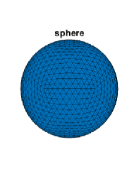
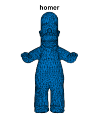
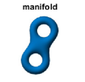
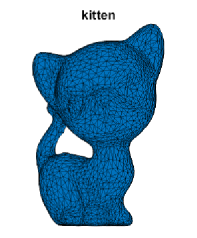
We follow a conventional approach to approximate a two-dimensional manifold 3superscript3\mathcal{M}\subset\mathbb{R}^{3} by a triangular mesh ~:={V,T}assign~𝑉𝑇\widetilde{\mathcal{M}}:=\{V,T\} [43, 30]. Here V={Vi3}i=1h𝑉superscriptsubscriptsubscript𝑉𝑖superscript3𝑖1V=\{{V_{i}}\in\mathbb{R}^{3}\}_{i=1}^{h} represents the set of vertices, T={Tj}j=1s𝑇superscriptsubscriptsubscript𝑇𝑗𝑗1𝑠T=\{{T_{j}}\}_{j=1}^{s} is the set of triangles where each triangle has three vertices in V𝑉V. Figure 1 shows several triangular meshes used in our numerical experiments later. For convenience, we also abuse our notation ~~\widetilde{\mathcal{M}} for the piecewise linear approximation of \mathcal{M} obtained from the the given triangular mesh.
Refer to caption
Refer to caption
Refer to caption
Figure 1: Triangular mesh approximation of some manifolds.

For a real-valued function ψ::𝜓\psi:\mathcal{M}\to\mathbb{R}, we approximate it with a piece-wise linear function Ψ:~:Ψ~\Psi:\widetilde{\mathcal{M}}\to\mathbb{R}, where on vertices Ψ(Vi):=ψ(Vi)assignΨsubscript𝑉𝑖𝜓subscript𝑉𝑖\Psi({V_{i}}):=\psi({V_{i}}) and on each triangle Ψ(𝐱)Ψ𝐱\Psi(\mathbf{x}) is linear. In this way, any piece-wise linear function on ~~\widetilde{\mathcal{M}} is fully represented by its values on vertices. With a slight abuse of notations, we denote Ψ:=(Ψ(V1)Ψ(Vh))assignΨmatrixΨsubscript𝑉1Ψsubscript𝑉\Psi:=\left(\begin{matrix}\Psi(V_{1})\\ \vdots\\ \Psi(V_{h})\end{matrix}\right) as a vector in hsuperscript\mathbb{R}^{h}. By piece-wise linearity, the gradient of ΨΨ\Psi is a piece-wise constant vector field. For consistency, we let T~:=j=1sspanTjassignT~superscriptsubscriptsquare-union𝑗1𝑠spansubscript𝑇𝑗\mathrm{T}\widetilde{\mathcal{M}}:=\sqcup_{j=1}^{s}\operatorname*{span}{{T_{j}}} mimic the tangent bundle, Γ(T~):={U:TT~,U(Tj)=(U1(Tj)U2(Tj)U3(Tj))spanTj}assignΓT~conditional-set𝑈formulae-sequence𝑇T~𝑈subscript𝑇𝑗matrixsuperscript𝑈1subscript𝑇𝑗superscript𝑈2subscript𝑇𝑗superscript𝑈3subscript𝑇𝑗spansubscript𝑇𝑗\Gamma(\mathrm{T}\widetilde{\mathcal{M}}):=\left\{U:T\to\mathrm{T}\widetilde{\mathcal{M}},U({T_{j}})=\left(\begin{matrix}U^{1}({T_{j}})\\ U^{2}({T_{j}})\\ U^{3}({T_{j}})\end{matrix}\right)\in\operatorname*{span}{{T_{j}}}\right\} denote the set of piece-wise constant vector field. Similar to the function discretization, we use the matrix U=(U1,U2,U3)=((U(T1))(U(Vs)))s×3𝑈matrixsuperscript𝑈1superscript𝑈2superscript𝑈3matrixsuperscript𝑈subscript𝑇1topsuperscript𝑈subscript𝑉𝑠topsuperscript𝑠3U=\left(\begin{matrix}U^{1},U^{2},U^{3}\end{matrix}\right)=\left(\begin{matrix}(U(T_{1}))^{\top}\\ \vdots\\ (U(V_{s}))^{\top}\end{matrix}\right)\in\mathbb{R}^{s\times 3} to fully describe the vector field.

Refer to caption
Refer to caption
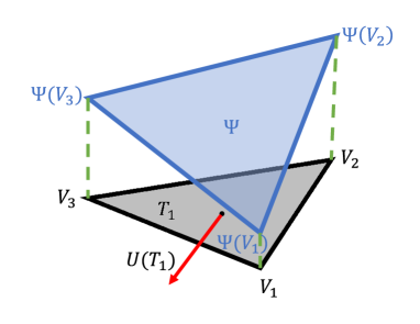
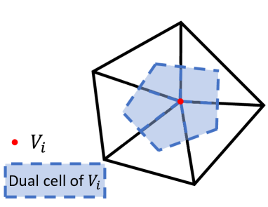
Figure 2: Illustration of definition of areas, functions and vector field on triangular meshes. (Left: gradient operator on one triangular face, right: dual cell of Visubscript𝑉𝑖{V_{i}}.)

Given any Ψ:~:Ψ~\Psi:\widetilde{\mathcal{M}}\to\mathbb{R}, its gradient ~ΨΓ(T~)subscript~ΨΓT~\nabla_{\widetilde{\mathcal{M}}}\Psi\in\Gamma(\mathrm{T}\widetilde{\mathcal{M}}) can be written as ~Ψ=(G1ΨG2ΨG3Ψ)subscript~Ψmatrixsuperscript𝐺1Ψsuperscript𝐺2Ψsuperscript𝐺3Ψ\nabla_{\widetilde{\mathcal{M}}}\Psi=\left(\begin{matrix}G^{1}\Psi&G^{2}\Psi&G^{3}\Psi\end{matrix}\right), where G1,G2,G3s×hsuperscript𝐺1superscript𝐺2superscript𝐺3superscript𝑠G^{1},G^{2},G^{3}\in\mathbb{R}^{s\times h} provides a discretization of subscript\nabla_{\mathcal{M}}. To see this, take a triangle T1subscript𝑇1T_{1} with vertices V1,V2,V3subscript𝑉1subscript𝑉2subscript𝑉3V_{1},V_{2},V_{3} as an example (see the left image in Figure 2). We first parameterise T1subscript𝑇1T_{1} by

V(ξ1,ξ2):=ξ1(V2V1)+ξ2(V3V1),0ξ1,ξ21,ξ1+ξ2=1.formulae-sequenceassign𝑉superscript𝜉1superscript𝜉2superscript𝜉1subscript𝑉2subscript𝑉1superscript𝜉2subscript𝑉3subscript𝑉1formulae-sequence0superscript𝜉1formulae-sequencesuperscript𝜉21superscript𝜉1superscript𝜉21V(\xi^{1},\xi^{2}):=\xi^{1}(V_{2}-V_{1})+\xi^{2}(V_{3}-V_{1}),\quad 0\leq\xi^{1},\xi^{2}\leq 1,\xi^{1}+\xi^{2}=1. (43)

Thus the induced metric on T1subscript𝑇1T_{1} is the constant matrix

g=(V2V1,V2V1V2V1,V3V1V3V1,V2V1V3V1,V3V1)𝑔matrixsubscript𝑉2subscript𝑉1subscript𝑉2subscript𝑉1subscript𝑉2subscript𝑉1subscript𝑉3subscript𝑉1subscript𝑉3subscript𝑉1subscript𝑉2subscript𝑉1subscript𝑉3subscript𝑉1subscript𝑉3subscript𝑉1g=\left(\begin{matrix}\langle V_{2}-V_{1},V_{2}-V_{1}\rangle&\langle V_{2}-V_{1},V_{3}-V_{1}\rangle\\ \langle V_{3}-V_{1},V_{2}-V_{1}\rangle&\langle V_{3}-V_{1},V_{3}-V_{1}\rangle\end{matrix}\right) (44)

Because ΨΨ\Psi restricted on T1subscript𝑇1T_{1} is linear, we have

Ψ(V(ξ1,ξ2)):=ξ1(Ψ(V2)Ψ(V1))+ξ2(Ψ(V3)Ψ(V1)).assignΨ𝑉superscript𝜉1superscript𝜉2superscript𝜉1Ψsubscript𝑉2Ψsubscript𝑉1superscript𝜉2Ψsubscript𝑉3Ψsubscript𝑉1\Psi(V(\xi^{1},\xi^{2})):=\xi^{1}(\Psi(V_{2})-\Psi(V_{1}))+\xi^{2}(\Psi(V_{3})-\Psi(V_{1})). (45)

The definition of gradient gives us

(V2V1,(~Ψ)(T1)V3V1,(~Ψ)(T1))matrixsubscript𝑉2subscript𝑉1subscript~Ψsubscript𝑇1subscript𝑉3subscript𝑉1subscript~Ψsubscript𝑇1\displaystyle\left(\begin{matrix}\langle V_{2}-V_{1},(\nabla_{\widetilde{\mathcal{M}}}\Psi)(T_{1})\rangle\\ \langle V_{3}-V_{1},(\nabla_{\widetilde{\mathcal{M}}}\Psi)(T_{1})\rangle\end{matrix}\right) =(Ψ(V2)Ψ(V1)Ψ(V3)Ψ(V1))=(110101)(Ψ(V1)Ψ(V2)Ψ(V3)).absentmatrixΨsubscript𝑉2Ψsubscript𝑉1Ψsubscript𝑉3Ψsubscript𝑉1matrix110101matrixΨsubscript𝑉1Ψsubscript𝑉2Ψsubscript𝑉3\displaystyle=\left(\begin{matrix}\Psi(V_{2})-\Psi(V_{1})\\ \Psi(V_{3})-\Psi(V_{1})\end{matrix}\right)=\left(\begin{matrix}-1&1&0\\ -1&0&1\end{matrix}\right)\left(\begin{matrix}\Psi(V_{1})\\ \Psi(V_{2})\\ \Psi(V_{3})\end{matrix}\right). (46)

Since (~Ψ)(T1)spanT1subscript~Ψsubscript𝑇1spansubscript𝑇1(\nabla_{\widetilde{\mathcal{M}}}\Psi)(T_{1})\in\operatorname*{span}{T_{1}}, it is clear that the gradient of ΨΨ\Psi on T1subscript𝑇1T_{1} has the decomposition (~Ψ)(T1)=(V2V1,V3V1)(μ1μ2)subscript~Ψsubscript𝑇1matrixsubscript𝑉2subscript𝑉1subscript𝑉3subscript𝑉1matrixsuperscript𝜇1superscript𝜇2(\nabla_{\widetilde{\mathcal{M}}}\Psi)(T_{1})=\left(\begin{matrix}V_{2}-V_{1},&V_{3}-V_{1}\end{matrix}\right)\left(\begin{matrix}\mu^{1}\\ \mu^{2}\end{matrix}\right) and therefore we have

(V2V1,(~Ψ)(T1)V3V1,(~Ψ)(T1))=g(μ1μ2)matrixsubscript𝑉2subscript𝑉1subscript~Ψsubscript𝑇1subscript𝑉3subscript𝑉1subscript~Ψsubscript𝑇1𝑔matrixsuperscript𝜇1superscript𝜇2\left(\begin{matrix}\langle V_{2}-V_{1},(\nabla_{\widetilde{\mathcal{M}}}\Psi)(T_{1})\rangle\\ \langle V_{3}-V_{1},(\nabla_{\widetilde{\mathcal{M}}}\Psi)(T_{1})\rangle\end{matrix}\right)=g\left(\begin{matrix}\mu^{1}\\ \mu^{2}\end{matrix}\right) (47)

Because the triangle is non-degenerative, (46) and (47) together solves μ1,μ2superscript𝜇1superscript𝜇2\mu^{1},\mu^{2}

(μ1μ2)=g1(110101)(Ψ(V1)Ψ(V2)Ψ(V3)).matrixsuperscript𝜇1superscript𝜇2superscript𝑔1matrix110101matrixΨsubscript𝑉1Ψsubscript𝑉2Ψsubscript𝑉3\displaystyle\left(\begin{matrix}\mu^{1}\\ \mu^{2}\end{matrix}\right)=g^{-1}\left(\begin{matrix}-1&1&0\\ -1&0&1\end{matrix}\right)\left(\begin{matrix}\Psi(V_{1})\\ \Psi(V_{2})\\ \Psi(V_{3})\end{matrix}\right). (48)

And this implies

(~Ψ)(T1)=(V2V1,V3V1)g1(110101)(Ψ(V1)Ψ(V2)Ψ(V3)).subscript~Ψsubscript𝑇1matrixsubscript𝑉2subscript𝑉1subscript𝑉3subscript𝑉1superscript𝑔1matrix110101matrixΨsubscript𝑉1Ψsubscript𝑉2Ψsubscript𝑉3\displaystyle(\nabla_{\widetilde{\mathcal{M}}}\Psi)(T_{1})=\left(\begin{matrix}V_{2}-V_{1},&V_{3}-V_{1}\end{matrix}\right)g^{-1}\left(\begin{matrix}-1&1&0\\ -1&0&1\end{matrix}\right)\left(\begin{matrix}\Psi(V_{1})\\ \Psi(V_{2})\\ \Psi(V_{3})\end{matrix}\right). (49)

Assigning Gd(T1,Vi)=0superscript𝐺𝑑subscript𝑇1subscript𝑉𝑖0G^{d}(T_{1},{V_{i}})=0 for ViV\{V1,V2,V3},d=1,2,3formulae-sequencesubscript𝑉𝑖\𝑉subscript𝑉1subscript𝑉2subscript𝑉3𝑑123{V_{i}}\in V\backslash\{V_{1},V_{2},V_{3}\},d=1,2,3 and

(G1(T1,V1)G1(T1,V2)G1(T1,V3)G2(T1,V1)G2(T1,V2)G2(T1,V3)G3(T1,V1)G3(T1,V2)G3(T1,V3))=(V2V1,V3V1)g1(110101)matrixsuperscript𝐺1subscript𝑇1subscript𝑉1superscript𝐺1subscript𝑇1subscript𝑉2superscript𝐺1subscript𝑇1subscript𝑉3superscript𝐺2subscript𝑇1subscript𝑉1superscript𝐺2subscript𝑇1subscript𝑉2superscript𝐺2subscript𝑇1subscript𝑉3superscript𝐺3subscript𝑇1subscript𝑉1superscript𝐺3subscript𝑇1subscript𝑉2superscript𝐺3subscript𝑇1subscript𝑉3matrixsubscript𝑉2subscript𝑉1subscript𝑉3subscript𝑉1superscript𝑔1matrix110101\displaystyle\left(\begin{matrix}G^{1}(T_{1},V_{1})&G^{1}(T_{1},V_{2})&G^{1}(T_{1},V_{3})\\ G^{2}(T_{1},V_{1})&G^{2}(T_{1},V_{2})&G^{2}(T_{1},V_{3})\\ G^{3}(T_{1},V_{1})&G^{3}(T_{1},V_{2})&G^{3}(T_{1},V_{3})\end{matrix}\right)=\left(\begin{matrix}V_{2}-V_{1},&V_{3}-V_{1}\end{matrix}\right)g^{-1}\left(\begin{matrix}-1&1&0\\ -1&0&1\end{matrix}\right) (50)

assures (~Ψ)(T1)=((G1Ψ)(T1)(G2Ψ)(T1)(G3Ψ)(T1))subscript~Ψsubscript𝑇1matrixsuperscript𝐺1Ψsubscript𝑇1superscript𝐺2Ψsubscript𝑇1superscript𝐺3Ψsubscript𝑇1(\nabla_{\widetilde{\mathcal{M}}}\Psi)(T_{1})=\left(\begin{matrix}(G^{1}\Psi)(T_{1})&(G^{2}\Psi)(T_{1})&(G^{3}\Psi)(T_{1})\end{matrix}\right). Following the same approach to define Gd(Tj,Vi)superscript𝐺𝑑subscript𝑇𝑗subscript𝑉𝑖G^{d}({T_{j}},{V_{i}}) on TjTsubscript𝑇𝑗𝑇{T_{j}}\in T, we have ~Ψ=(G1ΨG2ΨG3Ψ)subscript~Ψmatrixsuperscript𝐺1Ψsuperscript𝐺2Ψsuperscript𝐺3Ψ\nabla_{\widetilde{\mathcal{M}}}\Psi=\left(\begin{matrix}G^{1}\Psi&G^{2}\Psi&G^{3}\Psi\end{matrix}\right).

Next, we define discretization of the divergence operator based on its adjoint relation to the gradient operator. Consider the following discretization of surface area and inner product. Let ATjsubscript𝐴subscript𝑇𝑗A_{{T_{j}}} be the area of triangle Tjsubscript𝑇𝑗{T_{j}} and AVi:=13j:ViTjATjassignsubscript𝐴subscript𝑉𝑖13subscript:𝑗subscript𝑉𝑖subscript𝑇𝑗subscript𝐴subscript𝑇𝑗A_{{V_{i}}}:=\frac{1}{3}\sum_{j:{V_{i}}\in{T_{j}}}A_{{T_{j}}} be the area of the barycentric dual cell of Visubscript𝑉𝑖{V_{i}} (Figure 2 right), and denote AV:=diag(AV1,,AVh)h×hassignsubscript𝐴𝑉diagsubscript𝐴subscript𝑉1subscript𝐴subscript𝑉superscriptA_{V}:=\operatorname{diag}(A_{V_{1}},\cdots,A_{V_{h}})\in\mathbb{R}^{h\times h} and AT:=diag(AT1,,ATs)s×sassignsubscript𝐴𝑇diagsubscript𝐴subscript𝑇1subscript𝐴subscript𝑇𝑠superscript𝑠𝑠A_{T}:=\operatorname{diag}(A_{T_{1}},\cdots,A_{T_{s}})\in\mathbb{R}^{s\times s} be the mass matrices of vertices and of triangles. We then define the inner products of vector fields as U1,U2T:=tr(U1ATU2)=d=13(U1d)ATU2dassignsubscriptsubscript𝑈1subscript𝑈2𝑇trsuperscriptsubscript𝑈1topsubscript𝐴𝑇subscript𝑈2superscriptsubscript𝑑13superscriptsuperscriptsubscript𝑈1𝑑topsubscript𝐴𝑇superscriptsubscript𝑈2𝑑\langle U_{1},U_{2}\rangle_{T}:=\operatorname{tr}(U_{1}^{\top}A_{T}U_{2})=\sum_{d=1}^{3}(U_{1}^{d})^{\top}A_{T}U_{2}^{d} and of functions as Ψ1,Ψ2V:=Ψ1AVΨ2assignsubscriptsubscriptΨ1subscriptΨ2𝑉superscriptsubscriptΨ1topsubscript𝐴𝑉subscriptΨ2\langle\Psi_{1},\Psi_{2}\rangle_{V}:=\Psi_{1}^{\top}A_{V}\Psi_{2}. To preserve the adjoint relation between negative gradient and divergence under above inner products, i.e. ~Ψ,UT=Ψ,~UVsubscriptsubscript~Ψ𝑈𝑇subscriptΨsubscript~𝑈𝑉\langle-\nabla_{\widetilde{\mathcal{M}}}\Psi,U\rangle_{T}=\langle\Psi,\nabla_{\widetilde{\mathcal{M}}}\cdot U\rangle_{V}, we assign ~U:=d=13AV1(Gd)ATUdhassignsubscript~𝑈superscriptsubscript𝑑13superscriptsubscript𝐴𝑉1superscriptsuperscript𝐺𝑑topsubscript𝐴𝑇superscript𝑈𝑑superscript\nabla_{\widetilde{\mathcal{M}}}\cdot U:=-\sum_{d=1}^{3}A_{V}^{-1}(G^{d})^{\top}A_{T}U^{d}\in\mathbb{R}^{h}.

With the notations of area, we write the set of probability density functions on ~~\widetilde{\mathcal{M}} as 𝒫(~):={P+h:AVP=1}assign𝒫~conditional-set𝑃superscriptsubscriptsubscript𝐴𝑉𝑃1\mathcal{P}(\widetilde{\mathcal{M}}):=\{P\in\mathbb{R}_{+}^{h}:A_{V}P=1\}. If the the initial density is given as P0𝒫(~)subscript𝑃0𝒫~P_{0}\in\mathcal{P}(\widetilde{\mathcal{M}}), the semi-discrete constraint is then

ddtP(Vi,t)+(~M)(Vi,t)=0,P(,0)=P0,formulae-sequencedd𝑡𝑃subscript𝑉𝑖𝑡subscript~𝑀subscript𝑉𝑖𝑡0𝑃0subscript𝑃0\displaystyle\frac{\mathrm{d}}{\mathrm{d}t}P({V_{i}},t)+\left(\nabla_{\widetilde{\mathcal{M}}}\cdot M\right)({V_{i}},t)=0,P(\cdot,0)=P_{0}, (51)
PC([0,1];𝒫(V)),MC([0,1];Γ(T~)).formulae-sequence𝑃𝐶01𝒫𝑉𝑀𝐶01ΓT~\displaystyle P\in C([0,1];\mathcal{P}(V)),M\in C([0,1];\Gamma(\mathrm{T}\widetilde{\mathcal{M}})).

For the objective function, let W:hs:ΨΨ¯,Ψ¯(Tj)=w({ρ(Vi):ViTj}):𝑊superscriptsuperscript𝑠:formulae-sequencemaps-toΨ¯Ψ¯Ψsubscript𝑇𝑗𝑤conditional-set𝜌subscript𝑉𝑖subscript𝑉𝑖subscript𝑇𝑗W:\mathbb{R}^{h}\to\mathbb{R}^{s}:\Psi\mapsto\overline{\Psi},\quad\overline{\Psi}({T_{j}})=w(\{\rho({V_{i}}):{V_{i}}\in{T_{j}}\}) average the density values on each triangle. Below, we list some typical choices of w:=w({ρ(V1),ρ(V2),ρ(V3)})assign𝑤𝑤𝜌subscript𝑉1𝜌subscript𝑉2𝜌subscript𝑉3w:=w\left(\left\{\rho(V_{1}),\rho(V_{2}),\rho(V_{3})\right\}\right).

  • (i)

    Arithmetic mean:

    ω:=13iρ(Vi);assign𝜔13subscript𝑖𝜌subscript𝑉𝑖\omega:=\frac{1}{3}\sum_{i}\rho({V_{i}});
  • (ii)

    Geometric mean:

    w:=(iρ(Vi))13;assign𝑤superscriptsubscriptproduct𝑖𝜌subscript𝑉𝑖13w:=\left(\prod_{i}\rho({V_{i}})\right)^{\frac{1}{3}};
  • (iii)

    Harmonic mean:

    w:=3(i1ρ(Vi))1.assign𝑤3superscriptsubscript𝑖1𝜌subscript𝑉𝑖1w:=3\left(\sum_{i}\frac{1}{\rho({V_{i}})}\right)^{-1}.

We remark that these choices of average functions are useful in defining the related discrete mean-field variational problems. They connect with the gradient flow studies of Markov processes on discrete states. See related studies in [41]. For simplicity, we select the arithmetic mean (i) in this work.

We evaluate the dynamic cost on triangles L~:T~:~𝐿T~\widetilde{L}:\mathrm{T}\widetilde{\mathcal{M}}\to\mathbb{R}, and the interaction and terminal cost on vertices ~:𝒫(~):~𝒫~\widetilde{\mathcal{F}}:\mathcal{P}(\widetilde{\mathcal{M}})\to\mathbb{R}, T~:𝒫(~):~subscript𝑇𝒫~\widetilde{\mathcal{F}_{T}}:\mathcal{P}(\widetilde{\mathcal{M}})\to\mathbb{R}. With suitable choice of triangular mesh and discrete cost functions, the continuous cost is approximated by

𝒴~(P,M):=assign~𝒴𝑃𝑀absent\displaystyle\widetilde{\mathcal{Y}}(P,M):= 01j=1sATjP¯(Tj,t)L~(Tj,M(Tj,t)P¯(Tj,t))dt+01~(P(,t))dt+T~(P(,1)).superscriptsubscript01superscriptsubscript𝑗1𝑠subscript𝐴subscript𝑇𝑗¯𝑃subscript𝑇𝑗𝑡~𝐿subscript𝑇𝑗𝑀subscript𝑇𝑗𝑡¯𝑃subscript𝑇𝑗𝑡d𝑡superscriptsubscript01~𝑃𝑡differential-d𝑡~subscript𝑇𝑃1\displaystyle\int_{0}^{1}\sum_{j=1}^{s}A_{{T_{j}}}\overline{P}({T_{j}},t)\widetilde{L}\left({T_{j}},\frac{M({T_{j}},t)}{\overline{P}({T_{j}},t)}\right)\mathrm{d}t+\int_{0}^{1}\widetilde{\mathcal{F}}(P(\cdot,t))\mathrm{d}t+\widetilde{\mathcal{F}_{T}}(P(\cdot,1)). (52)

where P¯(,t)=W(P(,t))¯𝑃𝑡𝑊𝑃𝑡\overline{P}(\cdot,t)=W(P(\cdot,t)). The semi-discrete formulation of (28) on triangular mesh \mathcal{M} is then

minP,Msubscript𝑃𝑀\displaystyle\min_{P,M} 𝒴~(P,M)~𝒴𝑃𝑀\displaystyle\widetilde{\mathcal{Y}}(P,M) (53)
subject to ddtP(Vi,t)+(~M)(Vi,t)=0,P(,0)=P0,formulae-sequencedd𝑡𝑃subscript𝑉𝑖𝑡subscript~𝑀subscript𝑉𝑖𝑡0𝑃0subscript𝑃0\displaystyle\quad\frac{\mathrm{d}}{\mathrm{d}t}P({V_{i}},t)+\left(\nabla_{\widetilde{\mathcal{M}}}\cdot M\right)({V_{i}},t)=0,P(\cdot,0)=P_{0},
PC([0,1];𝒫(~)),MC([0,1];Γ(T~)).formulae-sequence𝑃𝐶01𝒫~𝑀𝐶01ΓT~\displaystyle\quad P\in C([0,1];\mathcal{P}(\widetilde{\mathcal{M}})),M\in C([0,1];\Gamma(\mathrm{T}\widetilde{\mathcal{M}})).
Remark 3.1.

Recall that in the continuous setting, we show that the local minimizer of the optimization problem (28) solves the PDE system (30) with F(𝐱,ρ(,t))=δ(ρ(,t))δρ(𝐱)𝐹𝐱𝜌𝑡𝛿𝜌𝑡𝛿𝜌𝐱F(\mathbf{x},\rho(\cdot,t))=\frac{\delta\mathcal{F}(\rho(\cdot,t))}{\delta\rho}(\mathbf{x}) and FT(𝐱,ρ(,1))=δT(ρ(,1))δρ(𝐱)subscript𝐹𝑇𝐱𝜌1𝛿subscript𝑇𝜌1𝛿𝜌𝐱F_{T}(\mathbf{x},\rho(\cdot,1))=\frac{\delta\mathcal{F}_{T}(\rho(\cdot,1))}{\delta\rho}(\mathbf{x}). Since the constraint of (53) remains linear, the local minimizer of this semi-discrete problem also solves a KKT-based ODE system

{ddtΦ(Vi,t)+j:ViTjATjAViP¯(Tj,t)P(Vi,t)H~(Tj,(~Φ)(Tj,t))1AViP(Vi)~(P(,t)),ddtP(Vi,t)+(~M)(Vi,t)=0,M(Tj,t)=P¯(Tj,t)QH~(Tj,(~Φ)(Tj,t)),Φ(Vi,1)1AViP(Vi)T~(P(,1)),P(,0)=P0.\left\{\begin{aligned} &-\frac{\mathrm{d}}{\mathrm{d}t}\Phi({V_{i}},t)+\sum_{j:{V_{i}}\in{T_{j}}}\frac{A_{{T_{j}}}}{A_{{V_{i}}}}\frac{\partial\overline{P}({T_{j}},t)}{\partial P({V_{i}},t)}\widetilde{H}\left({T_{j}},(\nabla_{\widetilde{\mathcal{M}}}\Phi)({T_{j}},t)\right)\leq\frac{1}{A_{{V_{i}}}}\partial_{P({V_{i}})}\widetilde{\mathcal{F}}(P(\cdot,t)),\\ &\frac{\mathrm{d}}{\mathrm{d}t}P({V_{i}},t)+\left(\nabla_{\widetilde{\mathcal{M}}}\cdot M\right)({V_{i}},t)=0,\quad M({T_{j}},t)=-\overline{P}({T_{j}},t)\partial_{Q}\widetilde{H}({T_{j}},(\nabla_{\widetilde{\mathcal{M}}}\Phi)({T_{j}},t)),\\ &\Phi({V_{i}},1)\leq\frac{1}{A_{{V_{i}}}}\partial_{P({V_{i}})}\widetilde{\mathcal{F}_{T}}(P(\cdot,1)),\quad P(\cdot,0)=P_{0}.\end{aligned}\right. (54)

where

H~:T~,H~(Tj,Q)=supU(Tj)spanTj{L~(Tj,U(Tj))Q,U(Tj)}.:~𝐻formulae-sequenceT~~𝐻subscript𝑇𝑗𝑄subscriptsupremum𝑈subscript𝑇𝑗spansubscript𝑇𝑗~𝐿subscript𝑇𝑗𝑈subscript𝑇𝑗𝑄𝑈subscript𝑇𝑗\widetilde{H}:\mathrm{T}\widetilde{\mathcal{M}}\to\mathbb{R},\widetilde{H}({T_{j}},Q)=\sup_{U({T_{j}})\in\operatorname*{span}{{T_{j}}}}\{-\widetilde{L}({T_{j}},U({T_{j}}))-\langle Q,U({T_{j}})\rangle\}.

Note that j:ViTjATjAViP¯(Tj,t)P(Vi,t)H~(Tj,(~Φ)(Tj,t))subscript:𝑗subscript𝑉𝑖subscript𝑇𝑗subscript𝐴subscript𝑇𝑗subscript𝐴subscript𝑉𝑖¯𝑃subscript𝑇𝑗𝑡𝑃subscript𝑉𝑖𝑡~𝐻subscript𝑇𝑗subscript~Φsubscript𝑇𝑗𝑡\displaystyle\sum_{j:{V_{i}}\in{T_{j}}}\frac{A_{{T_{j}}}}{A_{{V_{i}}}}\frac{\partial\overline{P}({T_{j}},t)}{\partial P({V_{i}},t)}\widetilde{H}\left({T_{j}},(\nabla_{\widetilde{\mathcal{M}}}\Phi)({T_{j}},t)\right) is an estimation of H(Vi,ϕ(Vi,t))𝐻subscript𝑉𝑖subscriptitalic-ϕsubscript𝑉𝑖𝑡H({V_{i}},\nabla_{\mathcal{M}}\phi({V_{i}},t)). If in addition, P(Vi)~(P(,t))/AVisubscript𝑃subscript𝑉𝑖~𝑃𝑡subscript𝐴subscript𝑉𝑖\partial_{P({V_{i}})}\widetilde{\mathcal{F}}(P(\cdot,t))/A_{{V_{i}}} and P(Vi)T~(P(,1))/AVisubscript𝑃subscript𝑉𝑖~subscript𝑇𝑃1subscript𝐴subscript𝑉𝑖\partial_{P({V_{i}})}\widetilde{\mathcal{F}_{T}}(P(\cdot,1))/A_{{V_{i}}} approximate the costs F(𝐱)𝐹𝐱F(\mathbf{x}) and FT(𝐱)subscript𝐹𝑇𝐱F_{T}(\mathbf{x}) evaluated at 𝐱=Vi𝐱subscript𝑉𝑖\mathbf{x}={V_{i}}, then (54) is a semi-discrete formulation of (30).

Before discretizing the time interval, we discuss the semi-discrete formulations of examples 2.9 and 2.10.

Example 3.2 (Quadratic dynamic cost with local interaction).

This is a discretized counterpart of example 2.9. Recall that in the continuous domain, Since we choose the surface metric as the induced metric, then for U(Tj)spanTj𝑈subscript𝑇𝑗spansubscript𝑇𝑗U({T_{j}})\in\operatorname*{span}{{T_{j}}}, the dynamic cost is provided as

L~(Tj,U(Tj))=12d=13(Ud(Tj))2=12U(Tj)32,~𝐿subscript𝑇𝑗𝑈subscript𝑇𝑗12superscriptsubscript𝑑13superscriptsuperscript𝑈𝑑subscript𝑇𝑗212superscriptsubscriptnorm𝑈subscript𝑇𝑗superscript32\widetilde{L}({T_{j}},U({T_{j}}))=\frac{1}{2}\sum_{d=1}^{3}(U^{d}({T_{j}}))^{2}=\frac{1}{2}\left\|U({T_{j}})\right\|_{\mathbb{R}^{3}}^{2}, (55)

And we approximate the interaction and terminal costs ,Tsubscript𝑇\mathcal{F},\mathcal{F}_{T} by

~(P(,t))=i=1hAViP(Vi,t)log(P(Vi,t)),~𝑃𝑡superscriptsubscript𝑖1subscript𝐴subscript𝑉𝑖𝑃subscript𝑉𝑖𝑡𝑃subscript𝑉𝑖𝑡\displaystyle\widetilde{\mathcal{F}}(P(\cdot,t))=\sum_{i=1}^{h}A_{{V_{i}}}P({V_{i}},t)\log(P({V_{i}},t)), (56)
T~(P(,1))=i=1hAViP(Vi,1)log(P(Vi,1)P1(Vi)).~subscript𝑇𝑃1superscriptsubscript𝑖1subscript𝐴subscript𝑉𝑖𝑃subscript𝑉𝑖1𝑃subscript𝑉𝑖1subscript𝑃1subscript𝑉𝑖\displaystyle\widetilde{\mathcal{F}_{T}}(P(\cdot,1))=\sum_{i=1}^{h}A_{{V_{i}}}P({V_{i}},1)\log\left(\frac{P({V_{i}},1)}{P_{1}({V_{i}})}\right).

With w𝑤w being the arithmetic average, if the optimizer P>0𝑃0P>0, then the discrete KKT system is

{ddtΦ(Vi,t)+j:ViTjATj3AVi12(~Φ)(Tj,t)32=log(P(Vi,t))+1,ddtP(Vi,t)+(~M)(Vi,t)=0,M(Tj,t)=P¯(Tj,t)(~Φ)(Tj,t),Φ(Vi,1)=log(P(Vi,1)P1(Vi)),P(,0)=P0.\left\{\begin{aligned} &-\frac{\mathrm{d}}{\mathrm{d}t}\Phi({V_{i}},t)+\sum_{j:{V_{i}}\in{T_{j}}}\frac{A_{{T_{j}}}}{3A_{{V_{i}}}}\frac{1}{2}\left\|(\nabla_{\widetilde{\mathcal{M}}}\Phi)({T_{j}},t)\right\|_{\mathbb{R}^{3}}^{2}=\log(P({V_{i}},t))+1,\\ &\frac{\mathrm{d}}{\mathrm{d}t}P({V_{i}},t)+\left(\nabla_{\widetilde{\mathcal{M}}}\cdot M\right)({V_{i}},t)=0,\quad M({T_{j}},t)=-\overline{P}({T_{j}},t)(\nabla_{\widetilde{\mathcal{M}}}\Phi)({T_{j}},t),\\ &\Phi({V_{i}},1)=\log\left(\frac{P({V_{i}},1)}{P_{1}({V_{i}})}\right),\quad P(\cdot,0)=P_{0}.\end{aligned}\right. (57)
Example 3.3 (Quadratic dynamic cost with non-local interaction cost).

This is a discretized counterpart of example 2.10. On triangular meshes, we use the following dynamic and terminal costs,

L~(Tj,U(Tj))=12U(Tj)32,~𝐿subscript𝑇𝑗𝑈subscript𝑇𝑗12superscriptsubscriptnorm𝑈subscript𝑇𝑗superscript32\displaystyle\widetilde{L}({T_{j}},U({T_{j}}))=\frac{1}{2}\left\|U({T_{j}})\right\|_{\mathbb{R}^{3}}^{2}, (58)
T~(P(,1))=i=1hAVi12(P(Vi,1)P1(Vi))2.~subscript𝑇𝑃1superscriptsubscript𝑖1subscript𝐴subscript𝑉𝑖12superscript𝑃subscript𝑉𝑖1subscript𝑃1subscript𝑉𝑖2\displaystyle\widetilde{\mathcal{F}_{T}}(P(\cdot,1))=\sum_{i=1}^{h}A_{{V_{i}}}\frac{1}{2}(P({V_{i}},1)-P_{1}({V_{i}}))^{2}.

And for the discrete interaction cost, we choose d~(V1,V2)subscript𝑑~subscript𝑉1subscript𝑉2d_{\widetilde{\mathcal{M}}}(V_{1},V_{2}) being the length of the shortest path connecting V1,V2subscript𝑉1subscript𝑉2V_{1},V_{2} to approximate the geodesic distance,

d~(V1,V2)=min{k=1nVikVik13:n=0,1,,Vi0=V1,Vin=V2,k=1,,n, there exists Tjk such that Vik1,VikTjk,}.subscript𝑑~subscript𝑉1subscript𝑉2:superscriptsubscript𝑘1𝑛subscriptnormsubscript𝑉subscript𝑖𝑘subscript𝑉subscript𝑖𝑘1superscript3absentformulae-sequence𝑛01formulae-sequencesubscript𝑉subscript𝑖0subscript𝑉1subscript𝑉subscript𝑖𝑛subscript𝑉2missing-subexpressionformulae-sequencefor-all𝑘1𝑛 there exists subscript𝑇subscript𝑗𝑘 such that subscript𝑉subscript𝑖𝑘1subscript𝑉subscript𝑖𝑘subscript𝑇subscript𝑗𝑘d_{\widetilde{\mathcal{M}}}(V_{1},V_{2})=\min\left\{\begin{aligned} \sum_{k=1}^{n}\|V_{i_{k}}-V_{i_{k-1}}\|_{\mathbb{R}^{3}}:&n=0,1,\cdots,V_{i_{0}}=V_{1},V_{i_{n}}=V_{2},\\ &\forall k=1,\cdots,n,\text{ there exists }T_{j_{k}}\text{ such that }V_{i_{k-1}},V_{i_{k}}\in T_{j_{k}},\end{aligned}\right\}. (59)

And we define the kernel as K~(V1,V2)=μexp(1σd~2(V1,V2))~𝐾subscript𝑉1subscript𝑉2𝜇1𝜎superscriptsubscript𝑑~2subscript𝑉1subscript𝑉2\widetilde{K}(V_{1},V_{2})=\mu\exp\left(-\frac{1}{\sigma}d_{\widetilde{\mathcal{M}}}^{2}(V_{1},V_{2})\right) and the interaction cost as

~(P(,t))=12ihihAViP(Vi)K~(Vi,Vi)AViP(Vi)=12P(,t)AVK~AVP(,t).~𝑃𝑡12superscriptsubscript𝑖superscriptsubscriptsuperscript𝑖subscript𝐴subscript𝑉𝑖𝑃subscript𝑉𝑖~𝐾subscript𝑉𝑖subscript𝑉superscript𝑖subscript𝐴subscript𝑉superscript𝑖𝑃subscript𝑉superscript𝑖12𝑃superscript𝑡topsubscript𝐴𝑉~𝐾subscript𝐴𝑉𝑃𝑡\widetilde{\mathcal{F}}(P(\cdot,t))=\frac{1}{2}\sum_{i}^{h}\sum_{i^{\prime}}^{h}A_{{V_{i}}}P({V_{i}})\widetilde{K}(V_{i},V_{i^{\prime}})A_{V_{i^{\prime}}}P(V_{i^{\prime}})=\frac{1}{2}P(\cdot,t)^{\top}A_{V}\widetilde{K}A_{V}P(\cdot,t). (60)

Similarly, if w𝑤w is the arithmetic average and the optimizer P>0𝑃0P>0, the discrete KKT system is

{ddtΦ(Vi,t)+j:ViTjATj3AVi12(~Φ)(Tj,t)32=iK~(Vi,Vi)AViP(Vi),ddtP(Vi,t)+(~M)(Vi,t)=0,M(Tj,t)=P¯(Tj,t)(~Φ)(Tj,t),Φ(Vi,1)=P(Vi,1)P1(Vi),P(,0)=P0.\left\{\begin{aligned} &-\frac{\mathrm{d}}{\mathrm{d}t}\Phi({V_{i}},t)+\sum_{j:{V_{i}}\in{T_{j}}}\frac{A_{{T_{j}}}}{3A_{{V_{i}}}}\frac{1}{2}\left\|(\nabla_{\widetilde{\mathcal{M}}}\Phi)({T_{j}},t)\right\|_{\mathbb{R}^{3}}^{2}=\sum_{i^{\prime}}\widetilde{K}(V_{i},V_{i^{\prime}})A_{V_{i^{\prime}}}P(V_{i^{\prime}}),\\ &\frac{\mathrm{d}}{\mathrm{d}t}P({V_{i}},t)+\left(\nabla_{\widetilde{\mathcal{M}}}\cdot M\right)({V_{i}},t)=0,\quad M({T_{j}},t)=-\overline{P}({T_{j}},t)(\nabla_{\widetilde{\mathcal{M}}}\Phi)({T_{j}},t),\\ &\Phi({V_{i}},1)=P({V_{i}},1)-P_{1}({V_{i}}),\quad P(\cdot,0)=P_{0}.\end{aligned}\right. (61)

3.2 Time discretization

To numerically solve (53), we fully discretize the problem by dividing the time interval [0,1]01[0,1] into n𝑛n segments and let tk=knsubscript𝑡𝑘𝑘𝑛{t_{k}}=\frac{k}{n}. Now we consider the density on central time steps P={P(,tk)}k=1,,n(𝒫(~))n𝑃subscript𝑃subscript𝑡𝑘𝑘1𝑛superscript𝒫~𝑛P=\{P(\cdot,{t_{k}})\}_{k=1,\cdots,n}\in(\mathcal{P}(\widetilde{\mathcal{M}}))^{n} and the flux on staggered time steps M={M(,tk12)}k=1,,n(Γ(T~))n𝑀subscript𝑀subscript𝑡𝑘12𝑘1𝑛superscriptΓT~𝑛M=\{M(\cdot,{t_{k-\frac{1}{2}}})\}_{k=1,\cdots,n}\in(\Gamma(\mathrm{T}\widetilde{\mathcal{M}}))^{n}.

Let the time differential operator be

(~tP)(,tk12):={11/n(P(,tk)P(,tk1)),k=2,,n,11/n(P(,t1)P0()),k=1.assignsubscript~𝑡𝑃subscript𝑡𝑘12cases11𝑛𝑃subscript𝑡𝑘𝑃subscript𝑡𝑘1𝑘2𝑛11𝑛𝑃subscript𝑡1subscript𝑃0𝑘1(\widetilde{\partial}_{t}P)(\cdot,{t_{k-\frac{1}{2}}}):=\begin{cases}\frac{1}{1/n}(P(\cdot,{t_{k}})-P(\cdot,t_{k-1})),&\quad k=2,\cdots,n,\\ \frac{1}{1/n}(P(\cdot,t_{1})-P_{0}(\cdot)),&\quad k=1.\end{cases} (62)

Then the discrete constraint set 𝒞~(P0)~𝒞subscript𝑃0\widetilde{\mathcal{C}}(P_{0}) is

𝒞~(P0):={(P,M):(~tP)(Vi,tk12)+(~M)(Vi,tk12)=0,ViV,k=1,,nP𝒫(~))n,M(Γ(T~))n}.\widetilde{\mathcal{C}}(P_{0}):=\left\{\begin{aligned} (P,M):&~{}(\widetilde{\partial}_{t}P)({V_{i}},{t_{k-\frac{1}{2}}})+(\nabla_{\widetilde{\mathcal{M}}}\cdot M)({V_{i}},{t_{k-\frac{1}{2}}})=0,\forall{V_{i}}\in V,k=1,\cdots,n\\ &\quad P\in\mathcal{P}(\widetilde{\mathcal{M}}))^{n},M\in(\Gamma(\mathrm{T}\widetilde{\mathcal{M}}))^{n}\end{aligned}\right\}. (63)

Additionally, letting

P¯(,tk12)¯𝑃subscript𝑡𝑘12\displaystyle\overline{P}(\cdot,{t_{k-\frac{1}{2}}}) :=12W(P(,tk))+12W(P(,tk1)),k=1,,nformulae-sequenceassignabsent12𝑊𝑃subscript𝑡𝑘12𝑊𝑃subscript𝑡𝑘1𝑘1𝑛\displaystyle:=\frac{1}{2}W(P(\cdot,{t_{k}}))+\frac{1}{2}W(P(\cdot,t_{k-1})),\quad k=1,\cdots,n (64)
𝒴~(P,M)~𝒴𝑃𝑀\displaystyle\widetilde{\mathcal{Y}}(P,M) :=1nk=1nj=1sATjP¯(Tj,tk12)L(Tj,M(Tj,tk12)P¯(Tj,tk12))+1nk=1n1~(P(,tk))+T~(P(,tn)).assignabsent1𝑛superscriptsubscript𝑘1𝑛superscriptsubscript𝑗1𝑠subscript𝐴subscript𝑇𝑗¯𝑃subscript𝑇𝑗subscript𝑡𝑘12𝐿subscript𝑇𝑗𝑀subscript𝑇𝑗subscript𝑡𝑘12¯𝑃subscript𝑇𝑗subscript𝑡𝑘121𝑛superscriptsubscript𝑘1𝑛1~𝑃subscript𝑡𝑘~subscript𝑇𝑃subscript𝑡𝑛\displaystyle:=\frac{1}{n}\sum_{k=1}^{n}\sum_{j=1}^{s}A_{{T_{j}}}\overline{P}({T_{j}},{t_{k-\frac{1}{2}}})L\left({T_{j}},\frac{M({T_{j}},{t_{k-\frac{1}{2}}})}{\overline{P}({T_{j}},{t_{k-\frac{1}{2}}})}\right)+\frac{1}{n}\sum_{k=1}^{n-1}\widetilde{\mathcal{F}}(P(\cdot,{t_{k}}))+\widetilde{\mathcal{F}_{T}}(P(\cdot,{t_{n}})).

we formulate the discrete optimization problem as

minP,M𝒴~(P,M)+χ𝒞~(ρ0)(P,M).subscript𝑃𝑀~𝒴𝑃𝑀subscript𝜒~𝒞subscript𝜌0𝑃𝑀\displaystyle\min_{P,M}\widetilde{\mathcal{Y}}(P,M)+\chi_{\widetilde{\mathcal{C}}(\rho_{0})}(P,M). (65)

Here χ𝜒\chi is the indicator function χ𝒞(𝐱)={0,𝐱𝒞+,𝐱𝒞subscript𝜒𝒞𝐱cases0𝐱𝒞𝐱𝒞\chi_{\mathcal{C}}(\mathbf{x})=\left\{\begin{array}[]{cc}0,&\mathbf{x}\in\mathcal{C}\\ +\infty,&\mathbf{x}\not\in\mathcal{C}\end{array}\right. of a convex set 𝒞𝒞\mathcal{C}.

In the next section, we focus on solving the optimization problem (65).

4 Algorithm for Solving Variational MFGs on Triangular Meshes

In this section, we adapt the fast algorithm proposed in [52] to solve the discretized potential mean-field game (65). This algorithm is based on a proximal gradient method (PGD) [46, 7].

To solve (65), we conduct gradient descent on the smooth component 𝒴~~𝒴\widetilde{\mathcal{Y}} of the objective function and proximal descent on the non-smooth component χ𝒞~(P0)subscript𝜒~𝒞subscript𝑃0\chi_{\widetilde{\mathcal{C}}(P_{0})}. The gradient descent step is trivially

(P(l+12),M(l+12))=(P(l),M(l))η(l)P,M𝒴~(P(l),M(l))superscript𝑃𝑙12superscript𝑀𝑙12superscript𝑃𝑙superscript𝑀𝑙superscript𝜂𝑙subscript𝑃𝑀~𝒴superscript𝑃𝑙superscript𝑀𝑙\left(P^{(l+\frac{1}{2})},M^{(l+\frac{1}{2})}\right)=\left(P^{(l)},M^{(l)}\right)-\eta^{(l)}\nabla_{P,M}\widetilde{\mathcal{Y}}\left(P^{(l)},M^{(l)}\right) (66)

with stepsize η(l)superscript𝜂𝑙\eta^{(l)}. The proximal descent is exactly the projection to 𝒞~(P0)~𝒞subscript𝑃0\widetilde{\mathcal{C}}(P_{0}). Let the inner product in discrete spaces be

Ψ1,Ψ2(𝒫(~))n,subscriptΨ1subscriptΨ2superscript𝒫~𝑛\displaystyle\Psi_{1},\Psi_{2}\in(\mathcal{P}(\widetilde{\mathcal{M}}))^{n}, Ψ1,Ψ2V,t:=1nk=1nΨ1(,tk),Ψ2(,tk)V,assignsubscriptsubscriptΨ1subscriptΨ2𝑉𝑡1𝑛superscriptsubscript𝑘1𝑛subscriptsubscriptΨ1subscript𝑡𝑘subscriptΨ2subscript𝑡𝑘𝑉\displaystyle\langle\Psi_{1},\Psi_{2}\rangle_{V,t}:=\frac{1}{n}\sum_{k=1}^{n}\langle\Psi_{1}(\cdot,{t_{k}}),\Psi_{2}(\cdot,{t_{k}})\rangle_{V},
U1,U2(Γ(T~))n,subscript𝑈1subscript𝑈2superscriptΓT~𝑛\displaystyle U_{1},U_{2}\in(\Gamma(\mathrm{T}\widetilde{\mathcal{M}}))^{n}, U1,U2T,t:=1nk=1nU1(,tk12),U2(,tk12)T,assignsubscriptsubscript𝑈1subscript𝑈2𝑇𝑡1𝑛superscriptsubscript𝑘1𝑛subscriptsubscript𝑈1subscript𝑡𝑘12subscript𝑈2subscript𝑡𝑘12𝑇\displaystyle\langle U_{1},U_{2}\rangle_{T,t}:=\frac{1}{n}\sum_{k=1}^{n}\langle U_{1}(\cdot,{t_{k-\frac{1}{2}}}),U_{2}(\cdot,{t_{k-\frac{1}{2}}})\rangle_{T},

Then

(P(l+1),M(l+1))=proj𝒞~(P0)(P(l+12),M(l+12)):=argmin(P,M)𝒞~(P0)12PP(l+12)V,t2+12MM(l+12)T,t2superscript𝑃𝑙1superscript𝑀𝑙1subscriptproj~𝒞subscript𝑃0superscript𝑃𝑙12superscript𝑀𝑙12assignsubscriptargmin𝑃𝑀~𝒞subscript𝑃012subscriptsuperscriptnorm𝑃superscript𝑃𝑙122𝑉𝑡12subscriptsuperscriptnorm𝑀superscript𝑀𝑙122𝑇𝑡(P^{{(l+1)}},M^{{(l+1)}})=\operatorname{proj}_{\widetilde{\mathcal{C}}(P_{0})}(P^{{(l+\frac{1}{2})}},M^{{(l+\frac{1}{2})}}):=\operatorname*{argmin}_{(P,M)\in\widetilde{\mathcal{C}}(P_{0})}\frac{1}{2}\left\|P-P^{{(l+\frac{1}{2})}}\right\|^{2}_{V,t}+\frac{1}{2}\left\|M-M^{{(l+\frac{1}{2})}}\right\|^{2}_{T,t} (67)

To solve the optimization problem (67), we introduce a dual variable Ψ={Ψ(,tk12)}k=1,,n(𝒫(~))nΨsubscriptΨsubscript𝑡𝑘12𝑘1𝑛superscript𝒫~𝑛\Psi=\{\Psi(\cdot,{t_{k-\frac{1}{2}}})\}_{k=1,\cdots,n}\in(\mathcal{P}(\widetilde{\mathcal{M}}))^{n} on vertices and the staggered time steps. The Lagrangian is therefore

𝒜(P,M,Ψ):=assign𝒜𝑃𝑀Ψabsent\displaystyle\mathcal{A}(P,M,\Psi):= 12PP(l+12)V,t2+12MM(l+12)T,t212subscriptsuperscriptnorm𝑃superscript𝑃𝑙122𝑉𝑡12subscriptsuperscriptnorm𝑀superscript𝑀𝑙122𝑇𝑡\displaystyle\frac{1}{2}\left\|P-P^{{(l+\frac{1}{2})}}\right\|^{2}_{V,t}+\frac{1}{2}\left\|M-M^{{(l+\frac{1}{2})}}\right\|^{2}_{T,t} (68)
+1nk=1nΨ(,tk12),(~tP)(,tk12)+~M(,tk12)V.1𝑛superscriptsubscript𝑘1𝑛subscriptΨsubscript𝑡𝑘12subscript~𝑡𝑃subscript𝑡𝑘12subscript~𝑀subscript𝑡𝑘12𝑉\displaystyle+\frac{1}{n}\sum_{k=1}^{n}\langle\Psi(\cdot,{t_{k-\frac{1}{2}}}),(\widetilde{\partial}_{t}P)(\cdot,{t_{k-\frac{1}{2}}})+\nabla_{\widetilde{\mathcal{M}}}\cdot M(\cdot,{t_{k-\frac{1}{2}}})\rangle_{V}.

If we define ~tsuperscriptsubscript~𝑡\widetilde{\partial}_{t}^{*} as

(~tΨ)(,tk):={11/n(Ψ(,tk12)Ψ(,tk+12)),k=1,2,,n1,11/nΨ(,tn12),k=n,assignsuperscriptsubscript~𝑡Ψsubscript𝑡𝑘cases11𝑛Ψsubscript𝑡𝑘12Ψsubscript𝑡𝑘12𝑘12𝑛111𝑛Ψsubscript𝑡𝑛12𝑘𝑛(\widetilde{\partial}_{t}^{*}\Psi)(\cdot,{t_{k}}):=\begin{cases}\frac{1}{1/n}(\Psi(\cdot,{t_{k-\frac{1}{2}}})-\Psi(\cdot,{t_{k+\frac{1}{2}}})),&k=1,2,\cdots,n-1,\\ \frac{1}{1/n}\Psi(\cdot,t_{n-\frac{1}{2}}),&k=n,\end{cases} (69)

then the Lagrangian is also

𝒜(P,M,Ψ):=assign𝒜𝑃𝑀Ψabsent\displaystyle\mathcal{A}(P,M,\Psi):= 12PP(l+12)V,t2+12MM(l+12)T,t212subscriptsuperscriptnorm𝑃superscript𝑃𝑙122𝑉𝑡12subscriptsuperscriptnorm𝑀superscript𝑀𝑙122𝑇𝑡\displaystyle\frac{1}{2}\left\|P-P^{{(l+\frac{1}{2})}}\right\|^{2}_{V,t}+\frac{1}{2}\left\|M-M^{{(l+\frac{1}{2})}}\right\|^{2}_{T,t} (70)
+1nk=1n(~tΨ)(,tk),P(,tk)VΨ(,t12),P0V1𝑛superscriptsubscript𝑘1𝑛subscriptsuperscriptsubscript~𝑡Ψsubscript𝑡𝑘𝑃subscript𝑡𝑘𝑉subscriptΨsubscript𝑡12subscript𝑃0𝑉\displaystyle+\frac{1}{n}\sum_{k=1}^{n}\langle(\widetilde{\partial}_{t}^{*}\Psi)(\cdot,{t_{k}}),P(\cdot,{t_{k}})\rangle_{V}-\langle\Psi(\cdot,t_{\frac{1}{2}}),P_{0}\rangle_{V}
+1nk=1n~Ψ(,tk12),M(,tk12)T.1𝑛superscriptsubscript𝑘1𝑛subscriptsubscript~Ψsubscript𝑡𝑘12𝑀subscript𝑡𝑘12𝑇\displaystyle+\frac{1}{n}\sum_{k=1}^{n}\langle-\nabla_{\widetilde{\mathcal{M}}}\Psi(\cdot,{t_{k-\frac{1}{2}}}),M(\cdot,{t_{k-\frac{1}{2}}})\rangle_{T}.

Thus the saddle point (P,M,Ψ)𝑃𝑀Ψ(P,M,\Psi) satisfies the linear system

(~tP)(,tk12)+~M(,tk12)=𝟎,k=1,,n.formulae-sequencesubscript~𝑡𝑃subscript𝑡𝑘12subscript~𝑀subscript𝑡𝑘120𝑘1𝑛(\widetilde{\partial}_{t}P)(\cdot,{t_{k-\frac{1}{2}}})+\nabla_{\widetilde{\mathcal{M}}}\cdot M(\cdot,{t_{k-\frac{1}{2}}})=\mathbf{0},\quad k=1,\cdots,n. (71)

and

{P(,tk)=P(l+12)(,tk)(~tΨ)(,tk),k=1,,nM(,tk12)=M(l+12)(,tk12)+~Ψ(,tk12),k=1,,n,\left\{\begin{aligned} P(\cdot,{t_{k}})&=P^{{(l+\frac{1}{2})}}(\cdot,{t_{k}})-(\widetilde{\partial}_{t}^{*}\Psi)(\cdot,{t_{k}}),\quad k=1,\cdots,n\\ M(\cdot,{t_{k-\frac{1}{2}}})&=M^{{(l+\frac{1}{2})}}(\cdot,{t_{k-\frac{1}{2}}})+\nabla_{\widetilde{\mathcal{M}}}\Psi(\cdot,{t_{k-\frac{1}{2}}}),\quad k=1,\cdots,n,\end{aligned}\right. (72)

Note that ~tsubscript~𝑡\widetilde{\partial}_{t} is a full rank operator, for k=1,,n𝑘1𝑛k=1,\cdots,n, Ψ(,tk12)Ψsubscript𝑡𝑘12\Psi(\cdot,{t_{k-\frac{1}{2}}}) is the unique solution to

(~t~tΨ)(,tk12)~~Ψ(,tk12)=(~tP(l+12))(,tk12)+~M(l+12)(,tk12).subscript~𝑡superscriptsubscript~𝑡Ψsubscript𝑡𝑘12subscript~subscript~Ψsubscript𝑡𝑘12subscript~𝑡superscript𝑃𝑙12subscript𝑡𝑘12subscript~superscript𝑀𝑙12subscript𝑡𝑘12(\widetilde{\partial}_{t}\widetilde{\partial}_{t}^{*}\Psi)(\cdot,{t_{k-\frac{1}{2}}})-\nabla_{\widetilde{\mathcal{M}}}\cdot\nabla_{\widetilde{\mathcal{M}}}\Psi(\cdot,{t_{k-\frac{1}{2}}})=(\widetilde{\partial}_{t}P^{{(l+\frac{1}{2})}})(\cdot,{t_{k-\frac{1}{2}}})+\nabla_{\widetilde{\mathcal{M}}}\cdot M^{{(l+\frac{1}{2})}}(\cdot,{t_{k-\frac{1}{2}}}). (73)

Since this linear solver is invariant to the data and the iteration number, in practice, we precompute it to save cost in the main iteration.

We summarize our algorithm in Alg. 1.

Algorithm 1 PGD for MFG on discrete mesh
  Parameters P0subscript𝑃0P_{0}
  Initialization P(0)(𝒫(~))nsuperscript𝑃0superscript𝒫~𝑛P^{(0)}\in(\mathcal{P}(\widetilde{\mathcal{M}}))^{n}, and M(0)(Γ(T~))nsuperscript𝑀0superscriptΓT~𝑛M^{(0)}\in(\Gamma(\mathrm{T}\widetilde{\mathcal{M}}))^{n}.
  for l=0,1,2,𝑙012l=0,1,2,\ldots do
     gradient descent
(P(l+12),M(l+12))=(P(l),M(l))η(l)P,M𝒴~(P(l),M(l))superscript𝑃𝑙12superscript𝑀𝑙12superscript𝑃𝑙superscript𝑀𝑙superscript𝜂𝑙subscript𝑃𝑀~𝒴superscript𝑃𝑙superscript𝑀𝑙\left(P^{(l+\frac{1}{2})},M^{(l+\frac{1}{2})}\right)=\left(P^{(l)},M^{(l)}\right)-\eta^{(l)}\nabla_{P,M}\widetilde{\mathcal{Y}}\left(P^{(l)},M^{(l)}\right)
     proximal descent for k=1,,n𝑘1𝑛k=1,\cdots,n, solve ΨΨ\Psi for
(~t~tΨ)(,tk12)~~Ψ(,tk12)=(~tP(l+12))(,tk12)+~M(l+12)(,tk12).subscript~𝑡superscriptsubscript~𝑡Ψsubscript𝑡𝑘12subscript~subscript~Ψsubscript𝑡𝑘12subscript~𝑡superscript𝑃𝑙12subscript𝑡𝑘12subscript~superscript𝑀𝑙12subscript𝑡𝑘12(\widetilde{\partial}_{t}\widetilde{\partial}_{t}^{*}\Psi)(\cdot,{t_{k-\frac{1}{2}}})-\nabla_{\widetilde{\mathcal{M}}}\cdot\nabla_{\widetilde{\mathcal{M}}}\Psi(\cdot,{t_{k-\frac{1}{2}}})=(\widetilde{\partial}_{t}P^{{(l+\frac{1}{2})}})(\cdot,{t_{k-\frac{1}{2}}})+\nabla_{\widetilde{\mathcal{M}}}\cdot M^{{(l+\frac{1}{2})}}(\cdot,{t_{k-\frac{1}{2}}}).
and conduct
{P(l+1)(,tk)=P(l+12)(,tk)(~tΨ)(,tk),k=1,,nM(l+1)(,tk12)=M(l+12)(,tk12)+~Ψ(,tk12),k=1,,n,\left\{\begin{aligned} P^{(l+1)}(\cdot,{t_{k}})&=P^{{(l+\frac{1}{2})}}(\cdot,{t_{k}})-(\widetilde{\partial}_{t}^{*}\Psi)(\cdot,{t_{k}}),\quad k=1,\cdots,n\\ M^{(l+1)}(\cdot,{t_{k-\frac{1}{2}}})&=M^{{(l+\frac{1}{2})}}(\cdot,{t_{k-\frac{1}{2}}})+\nabla_{\widetilde{\mathcal{M}}}\Psi(\cdot,{t_{k-\frac{1}{2}}}),\quad k=1,\cdots,n,\end{aligned}\right.
  end for

5 Numerical Examples

In this section, we conduct various experiments to show the effectiveness and flexibility of our mean-field game models on manifolds and the proposed numerical method. We provide numerical results on different manifolds. Most of these manifolds are non-Euclidean, thus conventional settings of mean-field games cannot handle them. In all of our experiments, we choose the induced metric for the manifold geometry, the quadratic dynamic cost L(Tj,U(Tj,t)):=12d(Ud(Tj,t))2assign𝐿subscript𝑇𝑗𝑈subscript𝑇𝑗𝑡12subscript𝑑superscriptsuperscript𝑈𝑑subscript𝑇𝑗𝑡2L\left({T_{j}},U({T_{j}},t)\right):=\frac{1}{2}\sum_{d}\left(U^{d}({T_{j}},t)\right)^{2}, and the arithmetic average w𝑤w. The interaction and terminal cost terms vary from examples and will be specified later. All of our numerical experiments are implemented in Matlab on a PC with an Intel(R) i7-8550U 1.80GHz CPU and 16 GB memory.

5.1 MFGs with local interactions

In this part, both \mathcal{F} and Tsubscript𝑇\mathcal{F}_{T} take local forms for all experiments.

The U.S. map based triangular mesh

We first consider a U.S. map based triangular mesh, which is the discretization of a subdomain on a spherical manifold. Assume that there are two obstacles on the map and it takes extra efforts for masses (agents) to pass through the obstacle region 𝒞~B~subscript~𝒞𝐵~\widetilde{\mathcal{C}}_{B}\subset\widetilde{\mathcal{M}}. We define B:~:𝐵~B:\widetilde{\mathcal{M}}\to\mathbb{R} be the piece-wise linear indicator of the obstacle with B(Vi)={1,Vi𝒞~B,0,Vi𝒞~B𝐵subscript𝑉𝑖cases1subscript𝑉𝑖subscript~𝒞𝐵0subscript𝑉𝑖subscript~𝒞𝐵B({V_{i}})=\begin{cases}1,&{V_{i}}\in\widetilde{\mathcal{C}}_{B},\\ 0,&{V_{i}}\in\widetilde{\mathcal{C}}_{B}\end{cases} (see Figure LABEL:fig:_usmap_result obstacle).

We pick the initial density P0subscript𝑃0P_{0} showed in Figure LABEL:fig:_usmap_result t=0𝑡0t=0. The mass concentrates in California. We let the mass to move freely during the time interval. To reflect the impact of the obstacle, we choose the interaction cost ~(P(,t))=50i=1hAViP(Vi,t)B(Vi)~𝑃𝑡50superscriptsubscript𝑖1subscript𝐴subscript𝑉𝑖𝑃subscript𝑉𝑖𝑡𝐵subscript𝑉𝑖\widetilde{\mathcal{F}}(P(\cdot,t))=50\sum_{i=1}^{h}A_{{V_{i}}}P({V_{i}},t)B({V_{i}}). We also encourage the mass to stop in the central and eastern part at the end. To achieve this, we define the terminal cost T~(P(,t))=110i=1hAViP(Vi,tn)BT(Vi)~subscript𝑇𝑃𝑡110superscriptsubscript𝑖1subscript𝐴subscript𝑉𝑖𝑃subscript𝑉𝑖subscript𝑡𝑛subscript𝐵𝑇subscript𝑉𝑖\widetilde{\mathcal{F}_{T}}(P(\cdot,t))=\frac{1}{10}\sum_{i=1}^{h}A_{{V_{i}}}P({V_{i}},t_{n})B_{T}({V_{i}}) with BT(Vi)={1,105Wthe longitude of Vi130W,0,otherwise.subscript𝐵𝑇subscript𝑉𝑖cases1superscript105Wthe longitude of subscript𝑉𝑖superscript130W0otherwiseB_{T}({V_{i}})=\begin{cases}1,&105^{\circ}\text{W}\leq\text{the longitude of }{V_{i}}\leq 130^{\circ}\text{W},\\ 0,&\text{otherwise}.\end{cases}

Our numerical results in Figure LABEL:fig:_usmap_result show that the density in the obstacle region remains low. This means the mass circumvent those areas very well. In addition, at t=1𝑡1t=1, the density in the central and eastern areas is generally denser than that in the western, which meets our expectation.

“8”-shape with obstacles

In this example, we demonstrate that our model and algorithm can successfully handle manifolds with complicated topology. We consider a “8” shape surface. Similarly as before, we assume there are obstacles on the manifold and the indicator of the obstacle B:~:𝐵~B:\widetilde{\mathcal{M}}\to\mathbb{R} is shown in Figure 4(a). In plots afterwards, we indicate the obstacle region with a different transparency. We pick the initial density P0subscript𝑃0P_{0} aggregating on the one end of “8” and the desired terminal density P1subscript𝑃1P_{1} on the other end (Figure 4(a)). For the interaction cost, we still choose ~(P(,t))=50i=1hAViP(Vi,t)B(Vi)~𝑃𝑡50superscriptsubscript𝑖1subscript𝐴subscript𝑉𝑖𝑃subscript𝑉𝑖𝑡𝐵subscript𝑉𝑖\widetilde{\mathcal{F}}(P(\cdot,t))=50\sum_{i=1}^{h}A_{{V_{i}}}P({V_{i}},t)B({V_{i}}) to avoid obstacle. And we write the terminal cost as T~(P(,t))=5i=1hAVi(P(Vi,1)P1(Vi))2~subscript𝑇𝑃𝑡5superscriptsubscript𝑖1subscript𝐴subscript𝑉𝑖superscript𝑃subscript𝑉𝑖1subscript𝑃1subscript𝑉𝑖2\widetilde{\mathcal{F}_{T}}(P(\cdot,t))=5\sum_{i=1}^{h}A_{{V_{i}}}\left(P({V_{i}},1)-P_{1}({V_{i}})\right)^{2} to push the terminal density P(,1)𝑃1P(\cdot,1) to the desired P1subscript𝑃1P_{1}.

Refer to caption
Refer to caption
Refer to caption
Refer to caption
(a) Illustration of the manifold, obstacle, initial density and terminal density
Refer to captionRefer to captionRefer to captionRefer to captionRefer to captionRefer to captionRefer to captionRefer to captionRefer to captionRefer to caption
(b) Snapshots of the evolution
Figure 4: Illustration of the model and snapshots of the density evolution.

We list the snapshots of resulting density evolution in Figure 4(b). These results show that the mass produced by our model successfully circumvents the obstacle on this genus-2 manifold. Additionally, the terminal density mainly aggregated in the support of P1subscript𝑃1P_{1} as we expect.

Irregular Euclidean domain

Besides introducing B𝐵B to impose a soft constraint of the obstacle, the general setup on manifolds enables us to have a different implementation for the hard obstacle constraints.

For example, consider an irregular Euclidean domain showed in Figure 5 with white regions punctured. Instead of handling the complicate boundary conditions when conducting mean-field game problems using conventional methods in Euclidean spaces, We view the region as a two-dimensional manifold and use a triangular mesh to approximate it. Then we directly apply our algorithm to the mesh without concerning the shape complexity.

The initial density P0subscript𝑃0P_{0} and desired terminal density P1subscript𝑃1P_{1} are approximations of two Gaussian distributions. And we choose terminal cost as T~(P(,t))=10i=1hAViP(Vi,1)log(P(Vi,1)P1(Vi))~subscript𝑇𝑃𝑡10superscriptsubscript𝑖1subscript𝐴subscript𝑉𝑖𝑃subscript𝑉𝑖1𝑃subscript𝑉𝑖1subscript𝑃1subscript𝑉𝑖\widetilde{\mathcal{F}_{T}}(P(\cdot,t))=10\sum_{i=1}^{h}A_{{V_{i}}}P({V_{i}},1)\log\left(\frac{P({V_{i}},1)}{P_{1}({V_{i}})}\right) to push P(,1)𝑃1P(\cdot,1) to P1subscript𝑃1P_{1}. In Figure 5, we compare the results with a vanilla interaction cost ~v(P(,t))=0subscript~𝑣𝑃𝑡0\widetilde{\mathcal{F}}_{v}(P(\cdot,t))=0 (Figure 5(a)) and with a disperse cost ~d(P(,t))=i=1hAViP(Vi,t)log(P(Vi,t))subscript~𝑑𝑃𝑡superscriptsubscript𝑖1subscript𝐴subscript𝑉𝑖𝑃subscript𝑉𝑖𝑡𝑃subscript𝑉𝑖𝑡\widetilde{\mathcal{F}}_{d}(P(\cdot,t))=\sum_{i=1}^{h}A_{{V_{i}}}P({V_{i}},t)\log(P({V_{i}},t)) (Figure 5(b)). We see that with ~dsubscript~𝑑\widetilde{\mathcal{F}}_{d}, the mass is prone to segregate during the evolution. To understand this, we refer to the original game description. With ~dsubscript~𝑑\widetilde{\mathcal{F}}_{d}, we actually solve a mean-field game with F(𝐱,ρ(,t))=log(ρ(𝐱,t))+1𝐹𝐱𝜌𝑡𝜌𝐱𝑡1F(\mathbf{x},\rho(\cdot,t))=\log(\rho(\mathbf{x},t))+1. To reduce the cost J𝐽J, agents prefer locations with lower F(𝐱,ρ(,t))𝐹𝐱𝜌𝑡F(\mathbf{x},\rho(\cdot,t)), i.e. lower density ρ(𝐱)𝜌𝐱\rho(\mathbf{x}).

Refer to caption
Refer to caption
Refer to caption
Refer to caption
Refer to caption
(a) MFG with vanilla ~v(P(,t))=0subscript~𝑣𝑃𝑡0\widetilde{\mathcal{F}}_{v}(P(\cdot,t))=0
Refer to caption
Refer to caption
Refer to caption
Refer to caption
Refer to caption
(b) MFG with disperse ~d(P(,t))=i=1hAViP(Vi,t)log(P(Vi,t))subscript~𝑑𝑃𝑡superscriptsubscript𝑖1subscript𝐴subscript𝑉𝑖𝑃subscript𝑉𝑖𝑡𝑃subscript𝑉𝑖𝑡\widetilde{\mathcal{F}}_{d}(P(\cdot,t))=\sum_{i=1}^{h}A_{{V_{i}}}P({V_{i}},t)\log(P({V_{i}},t))
Figure 5: Snapshots of MFGs with different interactions on constrained Euclidean space.

Homer surface

As the last example with local cost, we work with the surface of homer. We pick the initial density P0subscript𝑃0P_{0} concentrating on the belly and the desired terminal density P1subscript𝑃1P_{1} on the end of hands and feet. Fixing the terminal cost T~(P(,1))=52i=1hAVi(P(Vi,1)P1(Vi))2~subscript𝑇𝑃152superscriptsubscript𝑖1subscript𝐴subscript𝑉𝑖superscript𝑃subscript𝑉𝑖1subscript𝑃1subscript𝑉𝑖2\widetilde{\mathcal{F}_{T}}(P(\cdot,1))=\frac{5}{2}\sum_{i=1}^{h}A_{{V_{i}}}(P({V_{i}},1)-P_{1}({V_{i}}))^{2}, we compare the vanilla interaction cost ~v(P(,t))=0subscript~𝑣𝑃𝑡0\widetilde{\mathcal{F}}_{v}(P(\cdot,t))=0 and congested ~c(P(,t))=110i=1hAViP(Vi,t)+104subscript~𝑐𝑃𝑡110superscriptsubscript𝑖1subscript𝐴subscript𝑉𝑖𝑃subscript𝑉𝑖𝑡superscript104\widetilde{\mathcal{F}}_{c}(P(\cdot,t))=\frac{1}{10}\sum_{i=1}^{h}A_{{V_{i}}}\sqrt{P({V_{i}},t)+10^{-4}}. The choice of ~csubscript~𝑐\widetilde{\mathcal{F}}_{c} actually corresponds to the mean-field game with F(ρ(,t))=110ρ(𝐱,t)+104𝐹𝜌𝑡110𝜌𝐱𝑡superscript104F(\rho(\cdot,t))=\frac{1}{10\sqrt{\rho(\mathbf{x},t)+10^{4}}}. To reduce the cost during evolution, the agents tend to aggregate for a larger density value.

We solve the games with ~v,~csubscript~𝑣subscript~𝑐\widetilde{\mathcal{F}}_{v},\widetilde{\mathcal{F}}_{c} to obtain the local minimizers (Pv,Mv),(Pc,Mc)subscript𝑃𝑣subscript𝑀𝑣subscript𝑃𝑐subscript𝑀𝑐(P_{v},M_{v}),(P_{c},M_{c}) and report the corresponding dynamic cost, terminal cost and value of ~csubscript~𝑐\widetilde{\mathcal{F}}_{c} in Table 1. We also show and compare Pv(,t),Pc(,t)subscript𝑃𝑣𝑡subscript𝑃𝑐𝑡P_{v}(\cdot,t),P_{c}(\cdot,t) at several time steps in Figure 6. The costs in Table 1 show that our algorithm effectively reduce the interaction cost. From the snapshots, we observe that with the congested interaction cost, the mass move in a more compact manner.
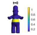
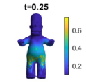
Refer to caption
Refer to caption
Refer to caption
Refer to caption
Refer to caption
(a) MFG with vanilla ~v(P(,t))=0subscript~𝑣𝑃𝑡0\widetilde{\mathcal{F}}_{v}(P(\cdot,t))=0
Refer to caption
Refer to caption
Refer to caption
Refer to caption
Refer to caption
(b) MFG with congested ~c(P(,t))=110i=1hAViP(Vi,t)+104subscript~𝑐𝑃𝑡110superscriptsubscript𝑖1subscript𝐴subscript𝑉𝑖𝑃subscript𝑉𝑖𝑡superscript104\widetilde{\mathcal{F}}_{c}(P(\cdot,t))=\frac{1}{10}\sum_{i=1}^{h}A_{{V_{i}}}\sqrt{P({V_{i}},t)+10^{-4}}
Figure 6: Snapshots of a MFG on the homer surface.
Table 1: Comparison of dynamic, interaction and terminal costs for experiments on the homer surface.
dynamic cost 1nk=1n1~c(P(,tk))1𝑛superscriptsubscript𝑘1𝑛1subscript~𝑐𝑃subscript𝑡𝑘\frac{1}{n}\sum_{k=1}^{n-1}\widetilde{\mathcal{F}}_{c}(P(\cdot,{t_{k}})) terminal cost
vanilla 0.0079 0.0393 5.5×1055.5superscript1055.5\times 10^{-5}
congested 0.0084 0.0378 8.2×1058.2superscript1058.2\times 10^{-5}

5.2 MFGs with non-local interactions

In this part, we show some mean-field games with non-local interaction cost.

The unit Sphere

In this example, we work on the triangular mesh of the unit sphere in three-dimensional space. The initial density P0subscript𝑃0P_{0} and desired terminal density P1subscript𝑃1P_{1} are spherical Gaussian. Again, we use the terminal cost T~(P(,t))=0.5i=1hAViP(Vi,1)log(P(Vi,1)P1(Vi)).~subscript𝑇𝑃𝑡0.5superscriptsubscript𝑖1subscript𝐴subscript𝑉𝑖𝑃subscript𝑉𝑖1𝑃subscript𝑉𝑖1subscript𝑃1subscript𝑉𝑖\widetilde{\mathcal{F}_{T}}(P(\cdot,t))=0.5\sum_{i=1}^{h}A_{{V_{i}}}P({V_{i}},1)\log\left(\frac{P({V_{i}},1)}{P_{1}({V_{i}})}\right). We then compute the game with vanilla interaction cost ~v(P(,t))=0subscript~𝑣𝑃𝑡0\widetilde{\mathcal{F}}_{v}(P(\cdot,t))=0 and non-local ~n(P(,t))=25i=1hiAViP(Vi)K~(Vi,Vi)AViP(Vi)subscript~𝑛𝑃𝑡25superscriptsubscript𝑖1subscriptsuperscript𝑖subscript𝐴subscript𝑉𝑖𝑃subscript𝑉𝑖~𝐾subscript𝑉𝑖subscript𝑉superscript𝑖subscript𝐴subscript𝑉superscript𝑖𝑃subscript𝑉superscript𝑖\widetilde{\mathcal{F}}_{n}(P(\cdot,t))=25\sum_{i=1}^{h}\sum_{i^{\prime}}A_{{V_{i}}}P({V_{i}})\widetilde{K}(V_{i},V_{i^{\prime}})A_{V_{i^{\prime}}}P(V_{i^{\prime}}). The kernel is defined as

K~(Vi,Vi)=exp((arccosViVi)2/σ2).~𝐾subscript𝑉𝑖subscript𝑉superscript𝑖superscriptsuperscriptsubscript𝑉𝑖topsubscript𝑉superscript𝑖2superscript𝜎2\widetilde{K}({V_{i}},V_{i^{\prime}})=\exp\left(-(\arccos{{V_{i}}^{\top}V_{i^{\prime}}})^{2}/\sigma^{2}\right).

Here σ=0.1𝜎0.1\sigma=0.1 and ViVisuperscriptsubscript𝑉𝑖topsubscript𝑉superscript𝑖{V_{i}}^{\top}V_{i^{\prime}} is the inner product of the two vectors in Euclidean space and arccosViVisuperscriptsubscript𝑉𝑖topsubscript𝑉superscript𝑖\arccos{{V_{i}}^{\top}V_{i^{\prime}}} is the geodesic distance between Visubscript𝑉𝑖{V_{i}} and Visubscript𝑉superscript𝑖V_{i^{\prime}} on sphere. We use the ground truth geodesic distance for simplicity. One can also compute the shortest path on the mesh and store it when pre-processing the manifold. We conduct the quantitative and snapshot comparison in Table 2 and in Figure 7. The table shows our algorithm effectively leverage the dynamic, interaction and terminal cost when taking the non-local cost ~nsubscript~𝑛\widetilde{\mathcal{F}}_{n}. And the comparison in Figure 7 clearly illustrates that the non-local cost ~nsubscript~𝑛\widetilde{\mathcal{F}}_{n} encourages the dispersion of mass.
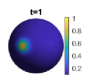
Refer to caption
Refer to caption
Refer to caption
Refer to caption
Refer to caption
(a) MFG with vanilla ~v(P(,t))=0subscript~𝑣𝑃𝑡0\widetilde{\mathcal{F}}_{v}(P(\cdot,t))=0.
Refer to caption
Refer to caption
Refer to caption
Refer to caption
Refer to caption
(b) MFG with non-local ~n(P(,t))=25i=1hiAViP(Vi)K~(Vi,Vi)AViP(Vi)subscript~𝑛𝑃𝑡25superscriptsubscript𝑖1subscriptsuperscript𝑖subscript𝐴subscript𝑉𝑖𝑃subscript𝑉𝑖~𝐾subscript𝑉𝑖subscript𝑉superscript𝑖subscript𝐴subscript𝑉superscript𝑖𝑃subscript𝑉superscript𝑖\widetilde{\mathcal{F}}_{n}(P(\cdot,t))=25\sum_{i=1}^{h}\sum_{i^{\prime}}A_{{V_{i}}}P({V_{i}})\widetilde{K}(V_{i},V_{i^{\prime}})A_{V_{i^{\prime}}}P(V_{i^{\prime}}).
Figure 7: Snapshots of MFGs with different interactions on sphere.
Table 2: Comparison of dynamic, interaction and terminal costs for experiments on sphere.
dynamic cost 1nk=1n1~n(P(,tk))1𝑛superscriptsubscript𝑘1𝑛1subscript~𝑛𝑃subscript𝑡𝑘\frac{1}{n}\sum_{k=1}^{n-1}\widetilde{\mathcal{F}}_{n}(P(\cdot,{t_{k}})) terminal cost
vanilla 0.0267 0.1220 0.0023
non-local 0.0292 0.1148 0.0039

Kitten

In the last example, we work with the kitten surface (Figure 8). Let the initial density P0subscript𝑃0P_{0} to concentrate on the paws and the desired terminal density on ears. We take the terminal cost T~(P(,1))=i=1hAVi(P(Vi,1)P1(Vi))2~subscript𝑇𝑃1superscriptsubscript𝑖1subscript𝐴subscript𝑉𝑖superscript𝑃subscript𝑉𝑖1subscript𝑃1subscript𝑉𝑖2\widetilde{\mathcal{F}_{T}}(P(\cdot,1))=\sum_{i=1}^{h}A_{{V_{i}}}\left(P({V_{i}},1)-P_{1}({V_{i}})\right)^{2} to push the mass moving from bottom to top. We also compare the non-local interaction cost ~n(P(,t))=12i=1hiAViP(Vi,t)K~(Vi,Vi)AViP(Vi,t)subscript~𝑛𝑃𝑡12superscriptsubscript𝑖1subscriptsuperscript𝑖subscript𝐴subscript𝑉𝑖𝑃subscript𝑉𝑖𝑡~𝐾subscript𝑉𝑖subscript𝑉superscript𝑖subscript𝐴subscript𝑉superscript𝑖𝑃subscript𝑉superscript𝑖𝑡\widetilde{\mathcal{F}}_{n}(P(\cdot,t))=\frac{1}{2}\sum_{i=1}^{h}\sum_{i^{\prime}}A_{{V_{i}}}P({V_{i}},t)\widetilde{K}(V_{i},V_{i^{\prime}})A_{V_{i^{\prime}}}P(V_{i^{\prime}},t) with the vanilla ~v(P(,t))=0subscript~𝑣𝑃𝑡0\widetilde{\mathcal{F}}_{v}(P(\cdot,t))=0 in Figure 8. The kernel is chosen as a weighted Laplacian matrix on the triangular mesh

K~(Vi,Vi)=1AVi1AVid=13j=1sATjGd(Tj,Vi)Gd(Tj,Vi).~𝐾subscript𝑉𝑖subscript𝑉superscript𝑖1subscript𝐴subscript𝑉𝑖1subscript𝐴subscript𝑉superscript𝑖superscriptsubscript𝑑13superscriptsubscript𝑗1𝑠subscript𝐴subscript𝑇𝑗superscript𝐺𝑑subscript𝑇𝑗subscript𝑉𝑖superscript𝐺𝑑subscript𝑇𝑗subscript𝑉superscript𝑖\widetilde{K}({V_{i}},V_{i^{\prime}})=\frac{1}{A_{{V_{i}}}}\frac{1}{A_{V_{i^{\prime}}}}\sum_{d=1}^{3}\sum_{j=1}^{s}A_{{T_{j}}}G^{d}({T_{j}},{V_{i}})G^{d}({T_{j}},V_{i^{\prime}}).

With this choice, the interaction cost is exactly

~n(P(,t))=12j=1sATj(~P)(Tj,tk)22,subscript~𝑛𝑃𝑡12superscriptsubscript𝑗1𝑠subscript𝐴subscript𝑇𝑗superscriptsubscriptnormsubscript~𝑃subscript𝑇𝑗subscript𝑡𝑘22\widetilde{\mathcal{F}}_{n}(P(\cdot,t))=\frac{1}{2}\sum_{j=1}^{s}A_{{T_{j}}}\left\|(\nabla_{\widetilde{\mathcal{M}}}P)({T_{j}},{t_{k}})\right\|_{2}^{2},

and approximates 12ρ(𝐱,t)g(𝐱)2d𝐱12subscriptsuperscriptsubscriptnormsubscript𝜌𝐱𝑡𝑔𝐱2subscriptd𝐱\frac{1}{2}\int_{\mathcal{M}}\left\|\nabla_{\mathcal{M}}\rho(\mathbf{x},t)\right\|_{g(\mathbf{x})}^{2}\mathrm{d}_{\mathcal{M}}\mathbf{x}. To reduce this cost, the density at each time step P(,tk)𝑃subscript𝑡𝑘P(\cdot,{t_{k}}) tends to be smooth on the space domain. The quantitative result in Table 3 shows the value 1nk=1n1~n(P(,tk))1𝑛superscriptsubscript𝑘1𝑛1subscript~𝑛𝑃subscript𝑡𝑘\frac{1}{n}\sum_{k=1}^{n-1}\widetilde{\mathcal{F}}_{n}(P(\cdot,{t_{k}})) is reduced by adding ~nsubscript~𝑛\widetilde{\mathcal{F}}_{n} to the objective function. And the comparisons of densities and colorbars in Figure 8 show that with ~nsubscript~𝑛\widetilde{\mathcal{F}}_{n} in objective function, at each time step, the density distributes more uniformly on the manifold.
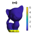
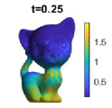
Refer to caption
Refer to caption
Refer to caption
Refer to caption
Refer to caption
(a) (vanilla) MFG with ~v(P(,t))=0subscript~𝑣𝑃𝑡0\widetilde{\mathcal{F}}_{v}(P(\cdot,t))=0
Refer to caption
Refer to caption
Refer to caption
Refer to caption
Refer to caption
(b) (non-local) MFG with ~n(P(,t))=12i=1hiAViP(Vi,t)K~(Vi,Vi)AViP(Vi,t)subscript~𝑛𝑃𝑡12superscriptsubscript𝑖1subscriptsuperscript𝑖subscript𝐴subscript𝑉𝑖𝑃subscript𝑉𝑖𝑡~𝐾subscript𝑉𝑖subscript𝑉superscript𝑖subscript𝐴subscript𝑉superscript𝑖𝑃subscript𝑉superscript𝑖𝑡\widetilde{\mathcal{F}}_{n}(P(\cdot,t))=\frac{1}{2}\sum_{i=1}^{h}\sum_{i^{\prime}}A_{{V_{i}}}P({V_{i}},t)\widetilde{K}(V_{i},V_{i^{\prime}})A_{V_{i^{\prime}}}P(V_{i^{\prime}},t)
Figure 8: Snapshots of MFGs with different interactions on “kitten”.
Table 3: Comparison of dynamic, interaction and terminal costs for experiments on “kitten”.
dynamic cost 1nk=1n1~n(P(,tk))1𝑛superscriptsubscript𝑘1𝑛1subscript~𝑛𝑃subscript𝑡𝑘\frac{1}{n}\sum_{k=1}^{n-1}\widetilde{\mathcal{F}}_{n}(P(\cdot,{t_{k}})) terminal cost
vanilla 0.5998 213.6033 0.0312
non-local 1.2429 0.6678 0.1710

5.3 Computation time and accuracy

At the end of this numerical section, we report the computation time and accuracy of above experiments in Table 4. As the computational complexity of our algorithm depends on the number of vertices hh and number of triangles s𝑠s on the mesh, we also include h,s𝑠h,s in the table.

As we mentioned in section 4, the proximal descent step requires solving a linear system (73). And since the linear solver is invariant to iteration numbers, we precompute it to reduce the total cost in the main iteration. The times reported in Table 4 include both the precomputation and the main iteration.

To show that our numerical result is close to the local minimizer of the fully discretized problem (65), we report the KKT residue in Table 4. To compute the KKT residue for a given output (P,M)𝑃𝑀(P,M), we first solve for Ψ={Ψ(,tk12)}k=1,,n(𝒫(~))nΨsubscriptΨsubscript𝑡𝑘12𝑘1𝑛superscript𝒫~𝑛\Psi=\{\Psi(\cdot,{t_{k-\frac{1}{2}}})\}_{k=1,\cdots,n}\in(\mathcal{P}(\widetilde{\mathcal{M}}))^{n} such that

~t~tΨ~~Ψ=~t(AV1P𝒴~(P,M))+~(AT1M𝒴~(P,M)).subscript~𝑡superscriptsubscript~𝑡Ψsubscript~subscript~Ψsubscript~𝑡superscriptsubscript𝐴𝑉1subscript𝑃~𝒴𝑃𝑀subscript~superscriptsubscript𝐴𝑇1subscript𝑀~𝒴𝑃𝑀\widetilde{\partial}_{t}\widetilde{\partial}_{t}^{*}\Psi-\nabla_{\widetilde{\mathcal{M}}}\cdot\nabla_{\widetilde{\mathcal{M}}}\Psi=\widetilde{\partial}_{t}(A_{V}^{-1}\partial_{P}\widetilde{\mathcal{Y}}(P,M))+\nabla_{\widetilde{\mathcal{M}}}\cdot(A_{T}^{-1}\partial_{M}\widetilde{\mathcal{Y}}(P,M)). (74)

Then let

{EP(Vi,tk):=min{1AViP(Vi,tk)𝒴~(P,M)(~tΨ)(Vi,tk),P(Vi,tk)},ViV,k=1,,nEM(Tj,tk):=1ATjM(Tj,tk12)𝒴~(P,M)+(~Ψ)(Tj,tk12)=0,TjT,k=1,,nEc(Vi,tk12):=(~tP)(Vi,tk12)+(~M)(Vi,tk12),ViV,k=1,,n.\left\{\begin{aligned} &E_{P}({V_{i}},{t_{k}}):=\min\left\{\frac{1}{A_{{V_{i}}}}\nabla_{P({V_{i}},{t_{k}})}\widetilde{\mathcal{Y}}(P,M)-(\widetilde{\partial}_{t}^{*}\Psi)({V_{i}},{t_{k}}),P({V_{i}},{t_{k}})\right\},\forall{V_{i}}\in V,k=1,\cdots,n\\ &E_{M}({T_{j}},{t_{k}}):=\frac{1}{A_{{T_{j}}}}\nabla_{M({T_{j}},{t_{k-\frac{1}{2}}})}\widetilde{\mathcal{Y}}(P,M)+(\nabla_{\widetilde{\mathcal{M}}}\Psi)({T_{j}},{t_{k-\frac{1}{2}}})=0,\forall{T_{j}}\in T,k=1,\cdots,n\\ &E_{c}({V_{i}},{t_{k-\frac{1}{2}}}):=(\widetilde{\partial}_{t}P)({V_{i}},{t_{k-\frac{1}{2}}})+(\nabla_{\widetilde{\mathcal{M}}}\cdot M)({V_{i}},{t_{k-\frac{1}{2}}}),\forall{V_{i}}\in V,k=1,\cdots,n.\end{aligned}\right. (75)

The KKT residue is defined as min{EPV,t,EMT,t,EcV,t}subscriptnormsubscript𝐸𝑃𝑉𝑡subscriptnormsubscript𝐸𝑀𝑇𝑡subscriptnormsubscript𝐸𝑐𝑉𝑡\min\{\|E_{P}\|_{V,t},\|E_{M}\|_{T,t},\|E_{c}\|_{V,t}\}. And P,M𝑃𝑀P,M is the local minimizer of (65), if and only if the KKT residue is 0.

Table 4: Computation time and accuracy
Triangle mesh and interaction cost hh s𝑠s time(s) number of iteration time(s) per iteration KKT residue
U.S. map 2900 5431 199.4813 3000 0.0665 3.15e-02
“8”-shape 766 1536 97.5769 5000 0.0195 1.70e-01
Irregular Euclidean vanilla 2473 4627 250.6317 5000 0.0501 1.49e-01
disperse 274.1786 0.0548 1.42e-01
Homer vanilla 2353 4702 163.2711 3000 0.0544 2.62e-03
congested 168.6198 0.0562 2.75e-03
Unit shpere vanilla 2562 5120 132.0967 2000 0.0660 6.27e-03
non-local 147.9476 0.0740 6.32e-03
Kitten vanilla 2884 5768 213.8950 3000 0.0713 2.99e-02
non-local 260.6147 0.0869 1.10e-01

6 Conclusion

In this work, we generalize mean-field games from Euclidean space to manifolds, design an optimization based algorithm to solve variational mean field games and conduct numerical experiments on various manifolds with triangular mesh representation. We first propose both the PDE formulation and the variational formulation of the Nash Equilibrium of a mean-field game. We also establish their equivalence on manifolds. To solve the potential mean-field games on manifolds, we use triangular meshes, piece-wise linear functions and piece-wise constant vector fields for discretization. Then we apply proximal gradient method to solve the corresponding discrete optimization problems. We conduct comprehensive numerical experiments to demonstrate flexibility of the model on handling different MFG problems on various manifolds.

References

  • [1] Yves Achdou, Francisco J Buera, Jean-Michel Lasry, Pierre-Louis Lions, and Benjamin Moll. Partial differential equation models in macroeconomics. Philosophical Transactions of the Royal Society A: Mathematical, Physical and Engineering Sciences, 372(2028):20130397, 2014.
  • [2] Yves Achdou, Fabio Camilli, and Italo Capuzzo-Dolcetta. Mean field games: convergence of a finite difference method. SIAM Journal on Numerical Analysis, 51(5):2585–2612, 2013.
  • [3] Yves Achdou and Italo Capuzzo-Dolcetta. Mean field games: numerical methods. SIAM Journal on Numerical Analysis, 48(3):1136–1162, 2010.
  • [4] Yves Achdou and Mathieu Laurière. Mean field games and applications: Numerical aspects. arXiv preprint arXiv:2003.04444, 2020.
  • [5] Noha Almulla, Rita Ferreira, and Diogo Gomes. Two numerical approaches to stationary mean-field games. Dynamic Games and Applications, 7(4):657–682, 2017.
  • [6] Heinz H Bauschke, Regina S Burachik, Patrick L Combettes, Veit Elser, D Russell Luke, and Henry Wolkowicz. Fixed-point algorithms for inverse problems in science and engineering, volume 49. Springer Science & Business Media, 2011.
  • [7] Amir Beck and Marc Teboulle. A fast iterative shrinkage-thresholding algorithm for linear inverse problems. SIAM journal on imaging sciences, 2(1):183–202, 2009.
  • [8] Jean-David Benamou and Guillaume Carlier. Augmented lagrangian methods for transport optimization, mean field games and degenerate elliptic equations. Journal of Optimization Theory and Applications, 167(1):1–26, 2015.
  • [9] Jean-David Benamou, Guillaume Carlier, and Filippo Santambrogio. Variational mean field games. In Active Particles, Volume 1, pages 141–171. Springer, 2017.
  • [10] Ariela Briani and Pierre Cardaliaguet. Stable solutions in potential mean field game systems. Nonlinear Differential Equations and Applications NoDEA, 25(1):1–26, 2018.
  • [11] Luis Briceño-Arias, Dante Kalise, Ziad Kobeissi, Mathieu Laurière, A Mateos González, and Francisco J Silva. On the implementation of a primal-dual algorithm for second order time-dependent mean field games with local couplings. ESAIM: Proceedings and Surveys, 65:330–348, 2019.
  • [12] Peter E Caines and Minyi Huang. Graphon mean field games and the gmfg equations. In 2018 IEEE Conference on Decision and Control (CDC), pages 4129–4134. IEEE, 2018.
  • [13] Pierre Cardaliaguet, P Jameson Graber, Alessio Porretta, and Daniela Tonon. Second order mean field games with degenerate diffusion and local coupling. Nonlinear Differential Equations and Applications NoDEA, 22(5):1287–1317, 2015.
  • [14] Guilherme Carmona. Nash equilibria of games with a continuum of players. 2004.
  • [15] René Carmona and Mathieu Laurière. Convergence analysis of machine learning algorithms for the numerical solution of mean field control and games: Ii–the finite horizon case. arXiv preprint arXiv:1908.01613, 2019.
  • [16] René Carmona, Mathieu Laurière, and Zongjun Tan. Model-free mean-field reinforcement learning: mean-field mdp and mean-field q-learning. arXiv preprint arXiv:1910.12802, 2019.
  • [17] Lawrence Cayton. Algorithms for manifold learning. Univ. of California at San Diego Tech. Rep, 12(1-17):1, 2005.
  • [18] Antonio De Paola, Vincenzo Trovato, David Angeli, and Goran Strbac. A mean field game approach for distributed control of thermostatic loads acting in simultaneous energy-frequency response markets. IEEE Transactions on Smart Grid, 10(6):5987–5999, 2019.
  • [19] Romuald Elie, Julien Perolat, Mathieu Laurière, Matthieu Geist, and Olivier Pietquin. On the convergence of model free learning in mean field games. In Proceedings of the AAAI Conference on Artificial Intelligence, volume 34, pages 7143–7150, 2020.
  • [20] Charles Fefferman, Sanjoy Mitter, and Hariharan Narayanan. Testing the manifold hypothesis. Journal of the American Mathematical Society, 29(4):983–1049, 2016.
  • [21] Wilfrid Gangbo, Wuchen Li, and Chenchen Mou. Geodesics of minimal length in the set of probability measures on graphs. ESAIM: COCV, 2019.
  • [22] Hao Gao, Wuchen Li, Miao Pan, Zhu Han, and H Vincent Poor. Modeling covid-19 with mean field evolutionary dynamics: Social distancing and seasonality. Journal of Communications and Networks, 23(5):314–325, 2021.
  • [23] Diogo Gomes and João Saúde. A mean-field game approach to price formation in electricity markets. arXiv preprint arXiv:1807.07088, 2018.
  • [24] Diogo A Gomes, Joana Mohr, and Rafael Rigao Souza. Continuous time finite state mean field games. Applied Mathematics & Optimization, 68(1):99–143, 2013.
  • [25] Diogo A Gomes and João Saúde. Numerical methods for finite-state mean-field games satisfying a monotonicity condition. Applied Mathematics & Optimization, 83(1):51–82, 2021.
  • [26] Olivier Guéant. Existence and uniqueness result for mean field games with congestion effect on graphs. Applied Mathematics & Optimization, 72(2):291–303, 2015.
  • [27] Minyi Huang, Peter E Caines, and Roland P Malhamé. Large-population cost-coupled lqg problems with nonuniform agents: individual-mass behavior and decentralized ε𝜀\varepsilon-nash equilibria. IEEE transactions on automatic control, 52(9):1560–1571, 2007.
  • [28] Minyi Huang, Roland P Malhamé, Peter E Caines, et al. Large population stochastic dynamic games: closed-loop mckean-vlasov systems and the nash certainty equivalence principle. Communications in Information & Systems, 6(3):221–252, 2006.
  • [29] H. W. Kuhn and A. W. Tucker. Nonlinear programming. In Proceedings of the Second Berkeley Symposium on Mathematical Statistics and Probability, pages 481–492. University of California Press, 1951.
  • [30] Rongjie Lai and Tony F Chan. A framework for intrinsic image processing on surfaces. Computer vision and image understanding, 115(12):1647–1661, 2011.
  • [31] Jean-Michel Lasry and Pierre-Louis Lions. Mean field games. Japanese journal of mathematics, 2(1):229–260, 2007.
  • [32] Mathieu Laurière. Numerical methods for mean field games and mean field type control. arXiv preprint arXiv:2106.06231, 2021.
  • [33] John M Lee. Smooth manifolds. In Introduction to Smooth Manifolds, pages 1–31. Springer, 2013.
  • [34] Taeyoung Lee, Melvin Leok, and N Harris McClamroch. Global formulations of lagrangian and hamiltonian dynamics on manifolds. Springer, 13:31, 2017.
  • [35] Wonjun Lee, Wuchen Li, and Stanley Osher. Mean field control problems for vaccine distribution. arXiv:2104.11887, 2021.
  • [36] Wonjun Lee, Siting Liu, Hamidou Tembine, Wuchen Li, and Stanley Osher. Controlling propagation of epidemics via mean-field control. SIAM Journal on Applied Mathematics, 81(1):190–207, 2021.
  • [37] Wuchen Li, Wonjun Lee, and Stanley Osher. Computational mean-field information dynamics associated with reaction diffusion equations. arXiv:2107.11501, 2021.
  • [38] Wuchen Li, Siting Liu, and Stanley Osher. Controlling conservation laws i: entropy-entropy flux. arXiv:2111.05473, 2021.
  • [39] Alex Tong Lin, Samy Wu Fung, Wuchen Li, Levon Nurbekyan, and Stanley J Osher. Apac-net: Alternating the population and agent control via two neural networks to solve high-dimensional stochastic mean field games. PNAS, 2021.
  • [40] Siting Liu, Matthew Jacobs, Wuchen Li, Levon Nurbekyan, and Stanley J Osher. Computational methods for first-order nonlocal mean field games with applications. SIAM Journal on Numerical Analysis, 59(5):2639–2668, 2021.
  • [41] Jan Maas. Gradient flows of the entropy for finite markov chains. Journal of Functional Analysis, 261(8):2250–2292, 2011.
  • [42] Olvi L Mangasarian. Pseudo-convex functions. In Stochastic optimization models in finance, pages 23–32. Elsevier, 1975.
  • [43] Mark Meyer, Mathieu Desbrun, Peter Schröder, and Alan H Barr. Discrete differential-geometry operators for triangulated 2-manifolds. In Visualization and mathematics III, pages 35–57. Springer, 2003.
  • [44] John Nash. Non-cooperative games. Annals of mathematics, pages 286–295, 1951.
  • [45] Levon Nurbekyan and Saúde João. Fourier approximation methods for first-order nonlocal mean-field games. Portugaliae Mathematica, 75(3):367–396, 2019.
  • [46] R Tyrrell Rockafellar. Convex analysis, volume 36. Princeton university press, 1970.
  • [47] Lars Ruthotto, Stanley J Osher, Wuchen Li, Levon Nurbekyan, and Samy Wu Fung. A machine learning framework for solving high-dimensional mean field game and mean field control problems. Proceedings of the National Academy of Sciences, 117(17):9183–9193, 2020.
  • [48] Justin Solomon, Gabriel Peyré, Vladimir G Kim, and Suvrit Sra. Entropic metric alignment for correspondence problems. ACM Transactions on Graphics (TOG), 35(4):1–13, 2016.
  • [49] E Weinan, Jiequn Han, and Qianxiao Li. A mean-field optimal control formulation of deep learning. Research in the Mathematical Sciences, 6(1):10, 2019.
  • [50] Chungang Yang, Jiandong Li, Min Sheng, Alagan Anpalagan, and Jia Xiao. Mean field game-theoretic framework for interference and energy-aware control in 5g ultra-dense networks. IEEE Wireless Communications, 25(1):114–121, 2017.
  • [51] Yaodong Yang, Rui Luo, Minne Li, Ming Zhou, Weinan Zhang, and Jun Wang. Mean field multi-agent reinforcement learning. In International Conference on Machine Learning, pages 5571–5580. PMLR, 2018.
  • [52] Jiajia Yu, Rongjie Lai, Wuchen Li, and Stanley Osher. A fast proximal gradient method and convergence analysis for dynamic mean field planning. arXiv preprint arXiv:2102.13260, 2021.