OmniXAI: A Library for Explainable AI

Abstract

We introduce OmniXAI (short for Omni eXplainable AI), an open-source Python library of eXplainable AI (XAI), which offers omni-way explainable AI capabilities and various interpretable machine learning techniques to address the pain points of understanding and interpreting the decisions made by machine learning (ML) in practice. OmniXAI aims to be a one-stop comprehensive library that makes explainable AI easy for data scientists, ML researchers and practitioners who need explanation for various types of data, models and explanation methods at different stages of a ML process (data exploration, feature engineering, model development, evaluation, and decision-making, etc). In particular, our library includes a rich family of explanation methods integrated in a unified interface, which supports multiple data types (tabular data, images, texts, time-series), multiple types of ML models (traditional ML in Scikit-learn and deep learning models in PyTorch/TensorFlow), and a range of diverse explanation methods including “model-specific” and “model-agnostic” ones (such as feature-attribution explanation, counterfactual explanation, gradient-based explanation, etc). For practitioners, the library provides an easy-to-use unified interface to generate the explanations for their applications by only writing a few lines of codes, and also a GUI dashboard for visualization of different explanations for more insights about decisions. In this technical report, we present OmniXAI’s design principles, system architectures, and major functionalities, and also demonstrate several example use cases across different types of data, tasks, and models.

Keywords: Explainable AI (XAI), Explainability, Counterfactual Explanation, Interpretable Machine Learning, Python, Scientific Toolkit

1 Introduction

With the rapidly growing adoption of machine learning (ML) models in real-world applications, the algorithmic decisions of ML models can potentially have a significant societal impact on building trustworthy AI systems for real-world applications, especially for some application domains such as healthcare, education, and finance, etc. Many ML models, especially deep learning models, work as black-box models that lack explainability and thus inhibit their adoption in some critical applications and hamper the trust in machine learning/AI systems. To address these challenges, eXplainable AI (XAI) is an emerging field in machine learning and AI, aiming to explain how those black-box decisions of AI systems are made. Such explanations can improve the transparency, persuasiveness, and trustworthiness of AI systems and help AI developers and practitioners to debug and improve model performance  (Doshi-Velez and Kim, 2017; Kusner et al., 2017; Lipton, 2016; Baniecki et al., 2021; Klaise et al., 2021).

To this end, we develop OmniXAI (short for Omni eXplainable AI), an open-source library for explainable AI to provide omni-way explainability for a variety of machine learning models.

Figure 1: OmniXAI offers explainablity for different stages in a standard ML workflow.

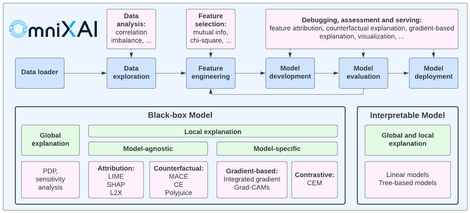
As shown in Figure 1, OmniXAI offers a one-stop solution for analyzing different stages in a standard ML workflow in real-world applications, and provides a comprehensive family of explanation methods, including high-quality implementations of various model-agnostic and model-specific explanation methods. In data analysis and exploration, OmniXAI can analyze feature correlations and data imbalance issues, helping developers quickly remove redundant features and discover potential bias issues. In feature engineering, OmniXAI can identify important features by analyzing relationships between features and targets, helping them understand data properties and do feature preprocessing. In model training and evaluation, OmniXAI provides various explanations, e.g., feature-attribution explanation, counterfactual explanation, gradient-based explanation, to comprehensively analyze the behavior of a model designed for tabular, vision, NLP, or time-series tasks. It helps to debug the model when wrong predictions occur or the model behavior is not as expected, and gathers more valuable information for improving feature engineering. After the model is deployed, OmniXAI opens “black boxes” and generates explanations for each model decision so that domain experts can analyze the decisions and explanations to determine which actions to take.

Compared with other existing explanation libraries, e.g., IBM’s AIX360 (Arya et al., 2019), Microsoft’s InterpretML (Nori et al., 2019), DALEX (Baniecki et al., 2021) and Alibi (Klaise et al., 2021), our library has a comprehensive list of XAI capabilities and unique features including:

• Support data analysis/exploration: we support feature analysis and selection, e.g., feature correlations, data imbalance issues, selecting important features.

• Support popular machine learning frameworks: we support the most popular machine learning frameworks or models, e.g., PyTorch, Tensorflow, scikit-learn and customized black-box models.

• Support most popular explanation methods: Many explanation methods, e.g., feature-attribution explanation, counterfactual explanation, partial dependence plots, etc., are included for analyzing different aspects of a machine learning model.

• Support explanations for tabular ranking tasks: We provide model-agnostic feature-attribution explanations for black-box learning-to-rank models. To the best of our knowledge, ours is the only library with this utility.

• Support counterfactual explanations: An efficient counterfactual explanation algorithm called MACE (model-agnostic counterfactual explanation) (Yang et al., 2022) designed for tabular and time-series data is included in the library. For text data, we include a method based on Polyjuice Wu et al. (2021) for text classification and question-answering tasks.

• Support gradient-based explanations: Integrated-gradient (Sundararajan et al., 2017), Grad-CAM (Selvaraju et al., 2019) and Grad-CAM’s variants (Chattopadhay et al., 2018) are supported.

• Support image, text, and time-series data: OmniXAI provides multiple explanation methods for a diverse set of tasks, e.g., Grad-CAM for vision tasks, integrated-gradient for NLP tasks, counterfactual for time-series tasks.

• Support feature visualization: OmniXAI supports feature visualization (an optimization-based method), and also provides ability to visualize feature maps for each layer.

• Easy-to-use: Users only need to write a few lines of code to generate various kinds of explanations, and OmniXAI supports Jupyter Notebook environments.

• Easy-to-extend: Developers can add new explanation algorithms easily by implementing a single class inherited from the explainer base class.

• A GUI dashboard: OmniXAI provides a visualization tool for users to examine the generated explanations and compare interpretability algorithms.

Table 1 shows the supported interpretability algorithms in OmniXAI, and Table 2 shows the comparison between OmniXAI and other existing XAI toolkits/libraries in literature. Our library supports all of these methods with a unified interface.

Table 1: The supported interpretability algorithms in OmniXAI

Method	Model Type	Exp Type	EDA	Tabular	Image	Text	TS
Feature analysis	NA	Global	✓
Feature selection	NA	Global	✓
Partial dependence plot	Black box	Global		✓
Accumulated local effects	Black box	Global		✓
Sensitivity analysis	Black box	Global		✓
Feature visualization	Torch or TF	Global			✓
LIME	Black box	Local		✓	✓	✓
SHAP	Black box*	Local		✓	✓	✓	✓
Integrated gradient	Torch or TF	Local		✓	✓	✓
Counterfactual	Black box*	Local		✓	✓	✓	✓
Contrastive explanation	Torch or TF	Local			✓
Grad-CAM	Torch or TF	Local			✓
Learning to explain	Black box	Local		✓	✓	✓
Linear models	Linear models	Global/local		✓
Tree models	Tree models	Global/local		✓
Feature maps	Torch or TF	Local			✓

Table 2: Comparison between OmniXAI and other XAI libraries.

Data Type	Method	OmniXAI	InterpretML	AIX360	Eli5	Captum	Alibi
Tabular	LIME	✓	✓	✓		✓
	SHAP	✓	✓	✓		✓	✓
	PDP	✓	✓
	ALE	✓					✓
	Sensitivity	✓	✓
	Integrated gradient	✓				✓	✓
	Counterfactual	✓					✓
	Linear models	✓	✓	✓	✓		✓
	Tree models	✓	✓	✓	✓		✓
	L2X	✓
Image	LIME	✓				✓
	SHAP	✓				✓
	Integrated gradient	✓				✓	✓
	Grad-CAM	✓			✓	✓
	CEM	✓		✓			✓
	Counterfactual	✓					✓
	L2X	✓
	Feature visualization	✓
Text	LIME	✓			✓	✓
	SHAP	✓				✓
	Integrated gradient	✓				✓	✓
	Counterfactual	✓
	L2X	✓
Timeseries	SHAP	✓
	Counterfactual	✓

The library includes a family of popular model-agnostic explanations methods (such as LIME (Ribeiro et al., 2016), SHAP (Lundberg and Lee, 2017), L2X (Chen et al., 2018)) and model-specific ones (e.g., integrated-gradient (IG) (Sundararajan et al., 2017)), which generate local explanations and can support multiple data types and tasks.

For tabular data, OmniXAI includes two methods for global explanations, i.e., partial dependence plot (PDP) (Hastie et al., 2001) and Morris sensitivity analysis (Morris, 1991) for analyzing how each feature affects model outcomes, and two counterfactual explanation methods, i.e., CE (Wachter et al., 2018) which can only handle continuous-valued features, and MACE (Yang et al., 2022) which is a model-agnostic method that can handle both continuous-valued and categorical features.

For image data, OmniXAI also supports Grad-CAM (Selvaraju et al., 2019), Grad-CAM++ (Chattopadhay et al., 2018) for explaining deep learning models on image domains, the contrastive explanation method (CEM) that finds pertinent negatives and pertinent positives for explanations, and the counterfactual explanation method CE (Wachter et al., 2018). Note that both CEM and CE only support the classification tasks.

For text data, in addition to the generic explanation methods (such as LIME, SHAP, and IG), OmniXAI also supports a counterfactual explanation method which is based on the pretrained model “Polyjuice” (Wu et al., 2021) for both classification and QA tasks.

Finally, for time-series data, OmniXAI supports explanation techniques for both time-series anomaly detection and time-series forecasting. Specifically, it provides a SHAP-based method and an optimization-based counterfactual explanation method MACE for both time-series anomaly detection and forecasting.

2 Library Design

Our key design principle is to provide a simple but unified interface allowing users to apply multiple explanation methods and visualize the corresponding generated explanations at the same time. This aims to make our library easy-to-use (generating explanations by writing a few lines of codes), easy-to-extend (adding new explanation methods easily without affecting the library framework), and easy-to-compare (visualizing the explanation results to compare multiple explanation methods). The library has five key components:

• Data classes – “omnixai.data”: This package contains the data classes for representing tabular data, image data, text data, and time-series data. For example, the explainers for tabular data use an instance of “omnixai.data.tabular” as one of their inputs. The library provides simple constructors for creating instances of these classes from numpy arrays, pandas dataframes, pillow images, or strings.

• Preprocessing modules – “omnixai.preprocessing”: This package contains various pre-processing functions for different data types. For example, it provides 1) one-hot encoding and ordinal encoding for categorical features, 2) KBins, standard normalization, min-max normalization, rescaling, NaN-filling for continuous-valued features, 3) rescaling, normalization, resizing for image data, and 4) the TF-IDF transformation and token-to-id transformation for text data.

• Explanation methods – “omnixai.explainers”: This is the main package in the library, which contains all the supported explainers. The explainers are categorized into four groups: 1) “omnixai.explainers.data” for data exploration/analysis, including feature correlation analysis, feature selection, etc., 2) “omnixai.explainers.tabular” for tabular data, e.g., global explanations such as PDP (Hastie et al., 2001), local explanations such as LIME (Ribeiro et al., 2016), SHAP (Lundberg and Lee, 2017), MACE (Yang et al., 2022), 3) “omnixai.explainers.vision” for vision tasks, e.g., integrated-gradient (Sundararajan et al., 2017), Grad-CAM (Selvaraju et al., 2019), contrastive explanation (Dhurandhar et al., 2018), counterfactual explanation (Wachter et al., 2018), and 4) “omnixai.explainers.nlp” for NLP tasks, e.g., LIME, integrated-gradient (IG).

  For each group, the explainers are further categorized into “model-agnostic”, “model-specific” and “counterfactual”. A “model-agnostic” explainer can handle black-box ML models, i.e., only requiring a prediction function without knowing model details. A “model-specific” explainer requires some information of ML models, e.g., whether the model is differentiable, whether the model is a linear model or a tree-based model. “Counterfactual” is a special group for counterfactual explanation methods.

• Explanation results – “omnixai.explanations”: This package contains the classes for explanation results. For example, the class “FeatureImportance” is used for storing feature-importance/attribution explanations. All of these classes provide plotting functions for visualization, e.g., “plot” using “Matplotlib”, “plotly_plot” using “Plotly Dash” and “ipython_plot” for Jupyter Notebook.

• Visualization tools – “omnixai.visualization”: This package contains a dashboard for visualization implemented using Plotly Dash. The dashboard supports both global explanations and local explanations. It provides a convenient way to compare and analyze multiple explanation results.

Figure 2 demonstrates the main architecture of the library. The package “omnixai.explainers” contains four special explainers, namely “TabularExplainer”, “VisionExplainer”, “NLPExplainer” and “TimeseriesExplainer”, inherited from “AutoExplainerBase” acting as the factories of the supported explainers. They provide a unified API for generating explanations with multiple explainers.

Figure 2: The main architecture of OmniXAI.

To initialize them, one only needs to specify the following parameters:

• The names of the explainers to apply: e.g., “shap” for SHAP, “pdp” for PDP, “gradcam” for Grad-CAM.

• The machine learning model to explain: e.g., a scikit-learn model, a tensorflow model, a pytorch model, or a black-box prediction function.

• The pre-processing function: e.g., converting raw input features into the model inputs, and feature processing.

• The post-processing function (optional): e.g., converting model outputs into class probabilities for classification tasks if the outputs are logits.

The class “AutoExplainerBase” will automatically check whether a chosen explainer is model-agnostic or model-specific and whether it generates local explanations or global explanations, and then determine how to call the method “explain” in the class “ExplainerBase” correctly to generate explanations. The generated explanations are stored in the explanation classes derived from “ExplanationBase” which has one method for extracting raw explanation results and three methods for visualization. One can call “plot”, “plotly_plot” or “ipython_plot” to visualize the explanations generated by each explainer separately, or launch a dashboard to visualize all the explanations at the same time to obtain more insights about the underlying model.

Figure 3: The pipeline for generating explanations in OmniXAI

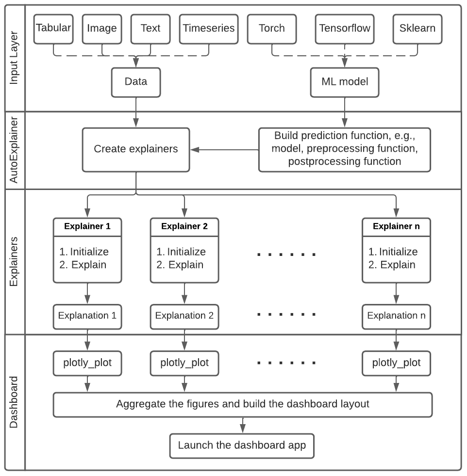
Figure 3 shows the pipeline for generating explanations.

Suppose we have a machine learning model to explain with the training dataset “tabular_data” and the feature processing function “transformer.transform”. Here is the sample code for creating a “TabularExplainer”.

⬇

1from omnixai.explainers.tabular import TabularExplainer

2# Initialize a TabularExplainer

3explainer = TabularExplainer(

4 explainers=["lime", "shap", "mace", "pdp"], # The explainers to apply

5 mode="classification", # The task type

6 data=tabular_data, # The data for initializing the explainers

7 model=model, # The machine learning model to explain

8 preprocess=preprocess, # Converting raw features into the model inputs

9 params={

10 "mace": {"ignored_features": ["Sex", "Race", "Relationship", "Capital Loss"]}

11 } # Additional parameters

12)

In this example, LIME, SHAP, and MACE generate local explanations while PDP generates global explanations. Given the test instances, “explainer.explain” returns the local explanations generated by the three methods, and “explainer.explain_global” returns the global explanations generated by PDP.

⬇

1# Generate local and global explanations

2local_explanations = explainer.explain(X=test_instances)

3global_explanations = explainer.explain_global()

Finally, given the generated explanations, we provide visualization tools to visualize the results. A dashboard can be configured by setting the test instances, the generated local explanations, the generated global explanations, the class names, and additional parameters for visualization (e.g., only plotting the selected features in PDP).

⬇

1from omnixai.visualization.dashboard import Dashboard

2# Launch a dashboard for visualization

3dashboard = Dashboard(

4 instances=test_instances, # The instances to explain

5 local_explanations=local_explanations, # Set the local explanations

6 global_explanations=global_explanations, # Set the global explanations

7 class_names=class_names, # Set class names

8 params={"pdp": {"features": ["Age", "Education-Num", "Capital Gain", "Capital Loss", "Hours per week", "Education", "Marital Status", "Occupation"]}}

9)

10dashboard.show() # Launch the dashboard

3 Supported Explanation Methods

There are two types of explanation methods, i.e., model-agnostic and model-specific. “Model-agnostic” means the methods can explain the decisions made by a black-box machine learning model without knowing the model details. “Model-specific” means the methods require some knowledge about the model to generate explanations, e.g., whether the model is a linear model or whether the model is differentiable w.r.t. its inputs. Model-specific methods provide more explanations about the decisions, e.g., the decision paths in a decision tree model.

3.1 Model-agnostic Explanation

The library treats all the methods for data analysis as model-agnostic methods because they analyze training/test data directly without using trained machine learning models, e.g., feature correlation analysis. Besides data analysis, some popular model-agnostic explanation methods, e.g., LIME (Ribeiro et al., 2016), SHAP (Lundberg and Lee, 2017), L2X (Chen et al., 2018), Partial Dependence Plots (PDP) (Hastie et al., 2001), and Morris sensitivity analysis (Morris, 1991) are included in the library. LIME, SHAP, and L2X generate local explanations, i.e., explaining a particular decision, while PDP and sensitivity analysis generate global explanations, i.e., explaining model behavior in general.

3.2 Model-specific Explanation

The model-specific methods in the library include gradient-based methods, e.g., the integrated-gradient (IG) method (Sundararajan et al., 2017), Grad-CAM (Selvaraju et al., 2019), etc., the contrastive explanation method (CEM) (Dhurandhar et al., 2018), and feature visualization. These methods need to compute the gradients of model outputs with respect to model inputs or particular internal layers, and thus require that the models to explain are neural networks implemented by PyTorch or Tensorflow. Different from gradient-based methods, CEM solves an optimization problem to compute pertinent negatives and pertinent positives for explanation, which can utilize numerical gradients instead of analytical gradients during optimization. Because computing numerical gradients is relatively expensive with high-dimensional data, our current CEM only supports differentiable models and thus is classified as a model-specific method. Future work will make CEM support gradient estimation methods for high-dimensional data.

3.3 Counterfactual Explanation

Counterfactual explanation interprets a model’s decision on a query instance by generating counterfactual examples that have minimal changes w.r.t the query instance’s features to yield a predefined output (Wachter et al., 2017; Moraffah et al., 2020; Byrne, 2019). It can not only explain the outcome of a model’s decision but also provide insight on how to change the outcome in the future. Although such methods can be grouped into “model-agnostic” and “model-specific”, we highlight them by creating a separate package in the library.

For tabular and time-series data, we recommend the recent MACE method (Yang et al., 2022) to generate counterfactual examples. MACE is a novel framework of model-agnostic counterfactual explanation, adopting a newly designed pipeline that can efficiently handle black-box machine learning models on a large number of feature values.

For image data, we choose the algorithm discussed in the paper (Wachter et al., 2018). This algorithm solves the following optimization problem given a query instance ${\bf x}$:

$$\min_{{\bf x}^{\prime}}\max_{\lambda}\lambda\mathcal{H}(f_{y}({\bf x}^{\prime})-\max_{y^{\prime}\neq y}f_{y^{\prime}}({\bf x}^{\prime}))+\|({\bf x}^{\prime}-{\bf x})\|_{1},$$ (1)

where $\mathcal{H}$ is the hinge loss function, $f_{y}({\bf x})$ represents the predicted class probability of sample ${\bf x}$ and label $y$, and the L1-norm regularization term is applied to encourage sparse modifications. Intuitively, it finds a counterfactual example ${\bf x}^{\prime}$ with a different predicted label from ${\bf x}$ and minimum changes of ${\bf x}$. This approach can also be applied to tabular data if all the features are continuous-valued.

For text data, we utilize the pretrained model “Polyjuice” (Wu et al., 2021) to generate a set of potential counterfactual examples for classification tasks and question-answering tasks, and then these examples are sorted based on whether the predicted labels/results are different from the original labels/results and the distances to the original texts.

4 Experiments

In this section, we present four sets of experiments to demonstrate the four major types of XAI capabilities in our library to deal with four types of real data.

4.1 XAI for Tabular Data: Income Prediction

The first experiment is to explain tabular data of an income prediction task. The dataset used in this example is the Adult dataset including 14 features, e.g., age, workclass, education. The goal is to predict whether income exceeds $50K per year on census data. We trained an XGBoost classifier (Chen and Guestrin, 2016) for this task, and then OmniXAI is applied to generate explanations for each prediction given test instances.

Figure 4: Dashboard visualization for income prediction

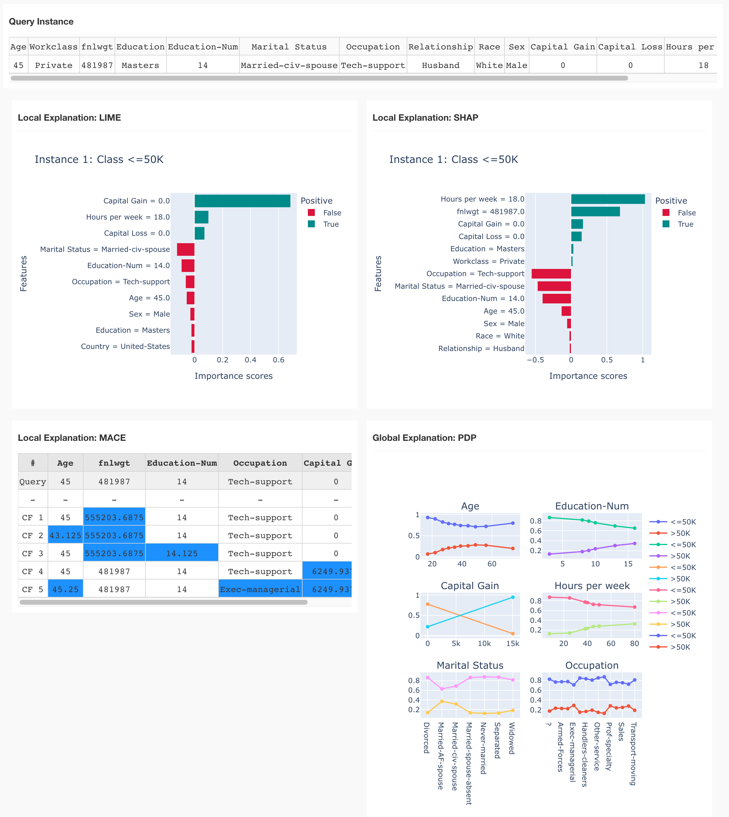
Figure 4 shows the explanation results generated by multiple explainers given a test instance, e.g., LIME, SHAP, MACE, and PDP. One can easily compare the feature-attribution explanations generated by LIME and SHAP, i.e., the predicted class is “$\leq 50k$” because “Hours per week = 18” (less than normal working hours), “Capital gain = 0” (no additional asset income), and “Captial loss” (people whose income is larger than 50k may have more investments). MACE generates counterfactual examples, exploring “what-if” scenarios and obtaining more insights of the underlying ML model, e.g., if “Capital gain” increases from 0 to 6249, the predicted class will be “$\geq 50k$” instead of “$\leq 50k$”. PDP explains the overall model behavior, e.g., income will increase as “Age” increase from 20 to 45 while income will decrease when “Age” increase from 45 to 80, longer working hours per week may lead to a higher income, and married people have a higher income (this is a potential bias in the dataset). From this dashboard, one can easily understand why such a prediction is made, whether there are potential issues in the dataset, and whether to do more feature processing/selection.

4.2 XAI for Vision: Image Classification

The second experiment is to explain an image classification task. We choose a ResNet (He et al., 2015) pretrained on ImageNet (Deng et al., 2009). Here is the sample code:

⬇

1explainer = VisionExplainer(

2 explainers=["lime", "ig",

3 "gradcam#0", "gradcam#3"],

4 mode="classification",

5 model=model, # A PyTorch ResNet50 model

6 preprocess=preprocess, # The preprocessing function

7 postprocess=postprocess, # The postprocessing function

8 params={

9 # Set the target layer

10 "gradcam#0": {"target_layer": model.layer4[-1]},

11 "gradcam#3": {"target_layer": model.layer4[-3]},

12 },

13)

14local_explanations = explainer.explain(

15 img,

16 # Explain a different label, e.g., "y=281" corresponds to "tiger_cat"

17 params={"gradcam#3": {"y": [281]}}

18)

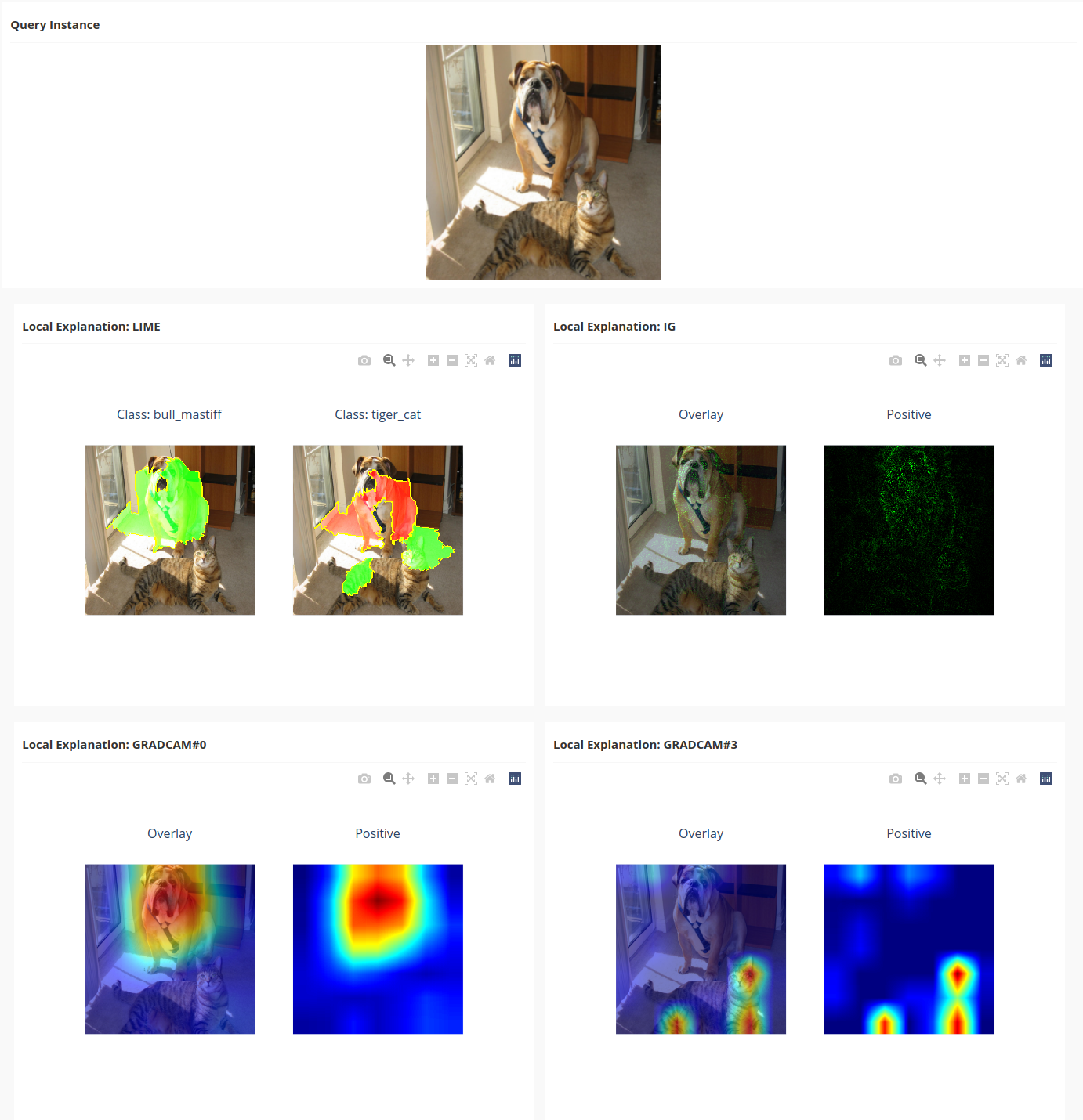
Figure 5 shows the explanations generated by multiple explainers, e.g., Grad-CAM, Integrated-gradient, LIME. The top predicted label of this test instance is “bull_mastiff”. These explainers explain the top predicted label by default (one can also set other labels to explain), e.g., integrated-gradient highlights the regions corresponding to “bull_mastiff”. Note that besides generating explanations with different explainers, OmniXAI can also generate explanations with the same explainer but different parameters. In this example, we apply Grad-CAM with different parameters, e.g., the target layer of “gradcam0” is “layer4[-1]” while the target layer of “gradcam3” is “layer4[-3]”, and the label to explain for the first Grad-CAM explainer is “bull_mastiff” (the top one label) while the label for the second Grad-CAM explainer is “tiger_cat”.

Figure 5: Dashboard visualization for image classification

Figure 6: Dashboard visualization for text classification

4.3 XAI for NLP: Sentiment Classification

The third experiment is to demonstrate the explanation for NLP tasks. Specifically, we consider a sentiment classification task on the IMDB dataset where the goal is to predict whether a user review is positive or negative. We train a text CNN model for this classification task using PyTorch, and then apply OmniXAI to generate explanations for each prediction given test instances. Suppose the processing function that converts the raw texts into the inputs of the model is "preprocess", and we want to analyze word/token importance and generate counterfactual examples. The following code shows how to do this:

⬇

1# The preprocessing function

2preprocess_func = lambda x: tuple(torch.tensor(y) for y in preprocess(x))

3# The postprocessing function

4postprocess_func = lambda logits: torch.nn.functional.softmax(logits, dim=1)

5# Initialize a NLPExplainer

6explainer = NLPExplainer(

7 explainers=["ig", "lime", "polyjuice"],

8 mode="classification",

9 model=model,

10 preprocess=preprocess_func,

11 postprocess=postprocess_func,

12 params={"ig":

13 # The embedding layer in the model

14 {"embedding_layer": model.embedding,

15 # For converting token ids into tokens

16 "id2token": id_to_token}}

17)

18

19x = Text("What a great movie! if you have no taste.")

20# Generates explanations

21local_explanations = explainer.explain(x)

22# Launch a dashboard for visualization

23dashboard = Dashboard(

24 instances=x,

25 local_explanations=local_explanations,

26 class_names=class_names

27)

28dashboard.show()

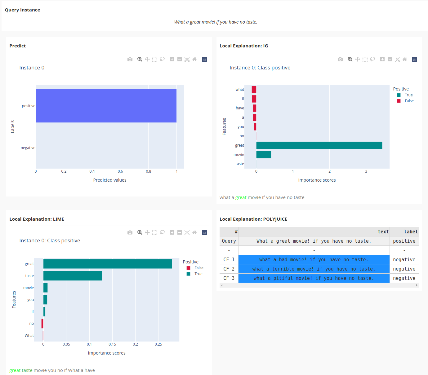
Figure 6 shows the explanation results generated by LIME, Integrated gradient (IG) and counterfactual explanation. Clearly, LIME and IG show that the word “great” has the largest word/token importance score, which implies that the sentence “What a great movie! if you have no taste.” is classified as “positive” because it contains “great”. The counterfactual method generates several counterfactual examples for this test sentence, e.g., “what a terrible movie! if you have no taste.”, helping us understand more about the model behavior.

Figure 7: Dashboard visualization for time-series anomaly detection.

4.4 XAI for Time-Series: Anomaly Detection

The last experiment is to explain time-series data. We consider a univariate time-series anomaly detection task. We use a simple statistics-based detector for demonstration, e.g., a window of time-series is detected as an anomaly according to some threshold estimated from the training data. Suppose we have detector “detector”, training data “train_df” and a test instance “test_df”. The following code shows how to apply OmniXAI in anomaly detection:

⬇

1# Initialize a TimeseriesExplainer

2explainers = TimeseriesExplainer(

3 explainers=["shap", "mace"], # Apply SHAP and MACE explainers

4 mode="anomaly_detection", # An anomaly detection task

5 data=Timeseries.from_pd(train_df), # Set data for initializing the explainers

6 model=detector, # Set the black-box anomaly detector

7 preprocess=None,

8 postprocess=None,

9 params={"mace": {"threshold": 0.001}} # Additional parameters for MACE

10)

11# Generate local explanations

12test_instance = Timeseries.from_pd(test_df)

13local_explanations = explainers.explain(test_instance)

14# Launch a dashboard for visualization

15dashboard = Dashboard(instances=test_instance, local_explanations=local_explanations)

16dashboard.show()

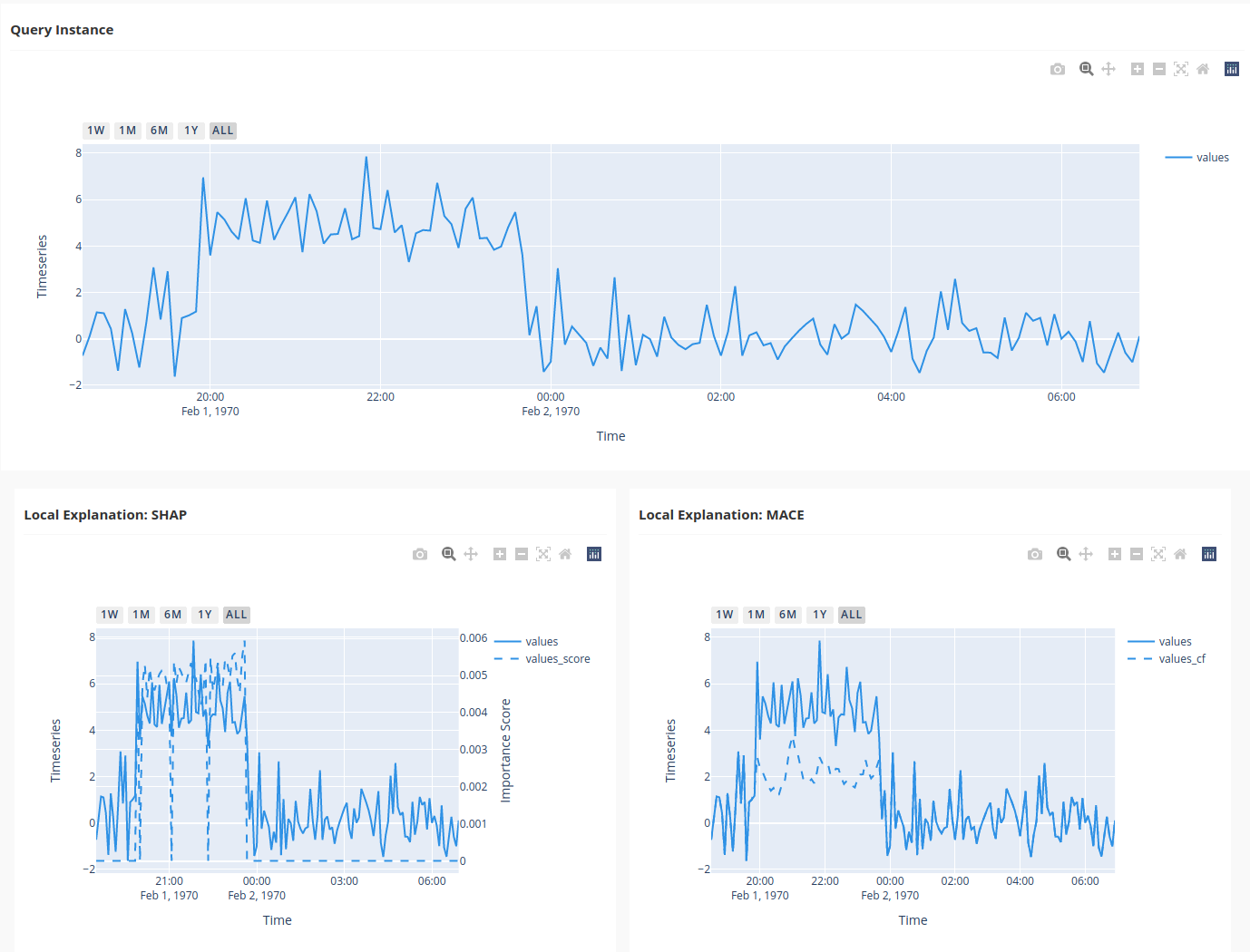
Figure 7 shows the explanation results generated by SHAP and MACE. The dash lines demonstrate the importance scores and the counterfactual examples, respectively. SHAP shows the most important timestamps that make this test instance detected as an anomaly. MACE provides a counterfactual example showing that it will not be detected as an anomaly if the metric values from 20:00 to 00:00 are around 2.0. From these two explanations, one can clearly understand the reason why the model considers it as an anomaly.

5 Broader Impacts and Responsible Use

The adoption of OmniXAI in real-world applications potentially can yield a broad range of positive impacts. OmniXAI offers a set of comprehensive and effective tools to interpret AI models and explain their decisions to improve the transparency and trustworthiness of AI systems, thus helping developers and users understand the logic behind the decisions. AI models sometimes may make unsatisfying or wrong decisions in real-world applications due to the data shift, sampling, labeling bias or other real data complexities. Explaining why an AI model fails is thus important and necessary, which is the key to keeping users confident in AI systems and help developers improve model performance. OmniXAI can be used to analyze various aspects of AI models and help developers figure out the issues and causes when a wrong decision occurs so that developers can quickly understand the reasons behind failures and improve the models accordingly. We encourage researchers, data scientists, and ML practitioners to adopt OmniXAI in real-world applications for positive impacts, e.g., improving transparency, accuracy, bias and fairness of AI/ML models.

While OmniXAI has many potential positive impacts, the misuse of OmniXAI may result in negative impacts. We encourage users and readers to read the detailed discussion and the guidelines for the responsible use of explainable ML in (Hall et al., 2019). In particular, the OmniXAI library should not be used to explain misused AI/ML models or any unethical use case. It also should not be used to enable hacking of models through public prediction API, or stealing black-box models or breaking privacy policies (Rudin, 2018; Tramèr et al., 2016; Shokri et al., 2019). For practical uses in real-world applications, we recommend using multiple explainers supported in OmniXAI, e.g., SHAP for feature-attribution explanation, MACE for counterfactual explanation, PDP for global explanation or “glass” models such as linear or tree-based models, for explaining a particular model decision to reduce the risk of adversarial manipulation. Finally, we note that while OmniXAI can help to understand and improve the sociological bias when used properly, it is not guaranteed to detect all kinds of sociological biases, which could be further improved in future work.

6 Conclusions and Future Work

We present OmniXAI, a comprehensive open-source library for explainable AI, which provides omni-way explanation capabilities to address many of the pain points in understanding and interpreting the decisions made by machine learning models. It supports various data types and tasks, and provides unified, easily extensible interfaces for a wide range of explanation methods, e.g., feature-attribution explanation, counterfactual explanation, gradient-based explanation, etc. It also includes a GUI dashboard for users to examine explanation results and compare different interpretable algorithms. We will continue our efforts to improve OmniXAI. Some planned future work includes adding more techniques for data analysis (e.g., detecting mislabeled samples and bias issues), adding more latest interpretable ML algorithms especially for NLP and time-series, and adding supports for other types of data and tasks. We will also improve the dashboard and user interface to make it easier to use and more comprehensive. Finally, we welcome any feedback and suggestions for improvement, and encourage contributions from the open-source communities.

References

- Arya et al. (2019) Vijay Arya, Rachel K. E. Bellamy, Pin-Yu Chen, Amit Dhurandhar, Michael Hind, Samuel C. Hoffman, Stephanie Houde, Q. Vera Liao, Ronny Luss, Aleksandra Mojsilović, Sami Mourad, Pablo Pedemonte, Ramya Raghavendra, John Richards, Prasanna Sattigeri, Karthikeyan Shanmugam, Moninder Singh, Kush R. Varshney, Dennis Wei, and Yunfeng Zhang. One explanation does not fit all: A toolkit and taxonomy of ai explainability techniques, 2019. URL https://arxiv.org/abs/1909.03012.
- Baniecki et al. (2021) Hubert Baniecki, Wojciech Kretowicz, Piotr Piatyszek, Jakub Wisniewski, and Przemyslaw Biecek. dalex: Responsible machine learning with interactive explainability and fairness in python. Journal of Machine Learning Research, 22(214):1–7, 2021. URL http://jmlr.org/papers/v22/20-1473.html.
- Byrne (2019) Ruth M. J. Byrne. Counterfactuals in explainable artificial intelligence (xai): Evidence from human reasoning. In Proceedings of the Twenty-Eighth International Joint Conference on Artificial Intelligence, IJCAI-19, pages 6276–6282. International Joint Conferences on Artificial Intelligence Organization, 7 2019. doi: 10.24963/ijcai.2019/876. URL https://doi.org/10.24963/ijcai.2019/876.
- Chattopadhay et al. (2018) Aditya Chattopadhay, Anirban Sarkar, Prantik Howlader, and Vineeth N Balasubramanian. Grad-cam++: Generalized gradient-based visual explanations for deep convolutional networks. In 2018 IEEE Winter Conference on Applications of Computer Vision (WACV), pages 839–847, 2018. doi: 10.1109/WACV.2018.00097.
- Chen et al. (2018) Jianbo Chen, Le Song, Martin J. Wainwright, and Michael I. Jordan. Learning to explain: An information-theoretic perspective on model interpretation, 2018.
- Chen and Guestrin (2016) Tianqi Chen and Carlos Guestrin. XGBoost: A scalable tree boosting system. In Proceedings of the 22nd ACM SIGKDD International Conference on Knowledge Discovery and Data Mining, KDD ’16, pages 785–794, New York, NY, USA, 2016. ACM. ISBN 978-1-4503-4232-2. doi: 10.1145/2939672.2939785. URL http://doi.acm.org/10.1145/2939672.2939785.
- Deng et al. (2009) Jia Deng, Wei Dong, Richard Socher, Li-Jia Li, Kai Li, and Li Fei-Fei. Imagenet: A large-scale hierarchical image database. In 2009 IEEE conference on computer vision and pattern recognition, pages 248–255. Ieee, 2009.
- Dhurandhar et al. (2018) Amit Dhurandhar, Pin-Yu Chen, Ronny Luss, Chun-Chen Tu, Paishun Ting, Karthikeyan Shanmugam, and Payel Das. Explanations based on the missing: Towards contrastive explanations with pertinent negatives, 2018.
- Doshi-Velez and Kim (2017) Finale Doshi-Velez and Been Kim. Towards a rigorous science of interpretable machine learning, 2017.
- Hall et al. (2019) Patrick Hall, Navdeep Gill, and Nicholas Schmidt. Proposed guidelines for the responsible use of explainable machine learning, 2019. URL https://arxiv.org/abs/1906.03533.
- Hastie et al. (2001) Trevor Hastie, Robert Tibshirani, and Jerome Friedman. The Elements of Statistical Learning. Springer Series in Statistics. Springer New York Inc., New York, NY, USA, 2001.
- He et al. (2015) Kaiming He, Xiangyu Zhang, Shaoqing Ren, and Jian Sun. Deep residual learning for image recognition. CoRR, abs/1512.03385, 2015. URL http://arxiv.org/abs/1512.03385.
- Klaise et al. (2021) Janis Klaise, Arnaud Van Looveren, Giovanni Vacanti, and Alexandru Coca. Alibi explain: Algorithms for explaining machine learning models. Journal of Machine Learning Research, 22(181):1–7, 2021. URL http://jmlr.org/papers/v22/21-0017.html.
- Kusner et al. (2017) Matt J Kusner, Joshua Loftus, Chris Russell, and Ricardo Silva. Counterfactual fairness. In I. Guyon, U. V. Luxburg, S. Bengio, H. Wallach, R. Fergus, S. Vishwanathan, and R. Garnett, editors, Advances in Neural Information Processing Systems 30, pages 4066–4076. Curran Associates, Inc., 2017. URL http://papers.nips.cc/paper/6995-counterfactual-fairness.pdf.
- Lipton (2016) Zachary Chase Lipton. The mythos of model interpretability. CoRR, abs/1606.03490, 2016. URL http://arxiv.org/abs/1606.03490.
- Lundberg and Lee (2017) Scott M Lundberg and Su-In Lee. A unified approach to interpreting model predictions. In I. Guyon, U. V. Luxburg, S. Bengio, H. Wallach, R. Fergus, S. Vishwanathan, and R. Garnett, editors, Advances in Neural Information Processing Systems 30, pages 4765–4774. Curran Associates, Inc., 2017.
- Moraffah et al. (2020) Raha Moraffah, Mansooreh Karami, Ruocheng Guo, Adrienne Raglin, and Huan Liu. Causal interpretability for machine learning - problems, methods and evaluation. SIGKDD Explor. Newsl., 22(1):18–33, May 2020. ISSN 1931-0145. doi: 10.1145/3400051.3400058. URL https://doi.org/10.1145/3400051.3400058.
- Morris (1991) Max D. Morris. Factorial sampling plans for preliminary computational experiments. Technometrics, 33(2):161–174, 1991. ISSN 00401706. URL http://www.jstor.org/stable/1269043.
- Nori et al. (2019) Harsha Nori, Samuel Jenkins, Paul Koch, and Rich Caruana. Interpretml: A unified framework for machine learning interpretability. arXiv preprint arXiv:1909.09223, 2019.
- Ribeiro et al. (2016) Marco Tulio Ribeiro, Sameer Singh, and Carlos Guestrin. “why should i trust you?”: Explaining the predictions of any classifier. In Proceedings of the 22nd ACM SIGKDD International Conference on Knowledge Discovery and Data Mining, KDD ’16, page 1135–1144, 2016.
- Rudin (2018) Cynthia Rudin. Stop explaining black box machine learning models for high stakes decisions and use interpretable models instead. 2018. doi: 10.48550/ARXIV.1811.10154. URL https://arxiv.org/abs/1811.10154.
- Selvaraju et al. (2019) Ramprasaath R. Selvaraju, Michael Cogswell, Abhishek Das, Ramakrishna Vedantam, Devi Parikh, and Dhruv Batra. Grad-cam: Visual explanations from deep networks via gradient-based localization. International Journal of Computer Vision, 128(2):336–359, Oct 2019. ISSN 1573-1405.
- Shokri et al. (2019) Reza Shokri, Martin Strobel, and Yair Zick. On the privacy risks of model explanations, 2019. URL https://arxiv.org/abs/1907.00164.
- Sundararajan et al. (2017) Mukund Sundararajan, Ankur Taly, and Qiqi Yan. Axiomatic attribution for deep networks. In Proceedings of the 34th International Conference on Machine Learning - Volume 70, ICML’17, page 3319–3328. JMLR.org, 2017.
- Tramèr et al. (2016) Florian Tramèr, Fan Zhang, Ari Juels, Michael K. Reiter, and Thomas Ristenpart. Stealing machine learning models via prediction apis, 2016. URL https://arxiv.org/abs/1609.02943.
- Wachter et al. (2017) S. Wachter, Brent D. Mittelstadt, and Chris Russell. Counterfactual explanations without opening the black box: Automated decisions and the gdpr. European Economics: Microeconomics & Industrial Organization eJournal, 2017.
- Wachter et al. (2018) S Wachter, BDM Mittelstadt, and C Russell. Counterfactual explanations without opening the black box: automated decisions and the gdpr. Harvard Journal of Law and Technology, 31(2):841–887, 2018.
- Wu et al. (2021) Tongshuang Wu, Marco Tulio Ribeiro, Jeffrey Heer, and Daniel Weld. Polyjuice: Generating counterfactuals for explaining, evaluating, and improving models. In Proceedings of the 59th Annual Meeting of the Association for Computational Linguistics and the 11th International Joint Conference on Natural Language Processing (Volume 1: Long Papers), pages 6707–6723, Online, August 2021. Association for Computational Linguistics. doi: 10.18653/v1/2021.acl-long.523. URL https://aclanthology.org/2021.acl-long.523.
- Yang et al. (2022) Wenzhuo Yang, Jia Li, Caiming Xiong, and Steven C. H. Hoi. Mace: An efficient model-agnostic framework for counterfactual explanation, 2022. URL https://arxiv.org/abs/2205.15540.