Finding Rule-Interpretable Non-Negative Data Representation

Abstract

Non-negative Matrix Factorization (NMF) is an intensively used technique for obtaining parts-based, lower dimensional and non-negative representation of non-negative data. It is a popular method in different research fields. Scientists performing research in the fields of biology, medicine and pharmacy often prefer NMF over other dimensionality reduction approaches (such as PCA) because the non-negativity of the approach naturally fits the characteristics of the domain problem and its result is easier to analyze and understand. Despite these advantages, it still can be hard to get exact characterization and interpretation of the NMF’s resulting latent factors due to their numerical nature. On the other hand, rule-based approaches are often considered more interpretable but lack the parts-based interpretation. In this work, we present a version of the NMF approach that merges rule-based descriptions with advantages of part-based representation offered by the NMF approach. Given the numerical input data with non-negative entries and a set of rules with high entity coverage, the approach creates the lower-dimensional non-negative representation of the input data in such a way that its factors are described by the appropriate subset of the input rules. In addition to revealing important attributes for latent factors, it allows analyzing relations between these attributes and provides the exact numerical intervals or categorical values they take. The proposed approach provides numerous advantages in tasks such as focused embedding or performing supervised multi-label NMF.

1 Introduction

Data analysis, as performed in various scientific fields, usually involves applying various techniques from statistics, data mining, machine learning and signal processing to obtain satisfactory results and insights in the given domain. Since the data typically has high dimensionality, it is often useful to decompose it into smaller components [6]. Multiple decomposition techniques have been developed for this task (e.g. SVD, PCA, NMF and ICA), each with its specific properties and goals [6].

Non-negative matrix factorization (NMF) [24, 19, 20] provides parts-based representation of the non-negative input data, often found in domains such as image processing, computer vision, biology, medicine or pharmacy. Many parameters in these domains have a natural representation with non-negative values, thus it makes sense to use the NMF approach to obtain latent factors. Non-negativity of the produced latent factors allows to partially obtain their meaning as the weighted sum of the attributes contained in the input data. Although very useful in many applications, this level of factor understanding is inadequate in some domains (e.g. biology or medicine), where more fine-grained interpretation – for instance, understanding a valid range of values in an attribute – is crucial for making informed decisions and appropriate conclusions. This problem has been slightly alleviated by the introduction of sparsity constraints, which aim to obtain adequate lower-dimensional data representation by keeping weights in factor representation either very close to $1$ or very close to $0$.

Sparsity, however, is not enough, and often identifying interesting groups of observations is preferable from interpretability’s point of view. Methods for this include, but are not limited to, clustering [7], inductive learning [21], subgroup discovery [18], redescription mining [26], anomaly detection [14] and many others. Each of these approaches have their special properties and advantages, which mostly provide deeper, interpretable understanding of some aspects of the studied domain. They identify groups of entities with some properties and many in addition offer rule-based descriptions. Although highly interpretable, these approaches are not without problems. Majority of the unsupervised rule-producing approaches construct very large rule-sets that are ultimately hard to explore. Structuring them is very beneficial when performing analyses. Predictive rule sets aim to produce smaller sets of rules, but this is not always achieved in practice. In addition, using rules as features, although shown to provide benefits for predictive models, necessarily increases the dimensionality of the original problem.

In this work, we aim to combine the advantages of both types of data analysis. The goal is to obtain non-negative part-based representation of the input data in such a way that the resulting factors are fully interpretable and represented by a number of rules obtained by any rule-producing approach. We propose a regularized NMF approach that takes a non-negative input data and a set of rules as input and produces a lower-dimensional data representation, where each latent factor is described by a number of input rules. Rules are either represented as a matrix, where rows denote entities and columns denote rules or the constraints derived from rules are written in the clustering matrix, where rows denote entities and columns denote clusters derived from rules. The approach provides novel insights and data analysis capabilities that were previously either hard or impossible to obtain, but are at the same time highly desirable and needed for research conducted in various scientific domains. These capabilities include exact interpretation of NMF latent factors (including exact numeric intervals or categorical values of attributes with the ability of observing and analyzing relations between attributes associated with a given factor), ability to perform guided embedding, combining multiple sources of information (for example, embedding genes belonging to a selected subset of organisms and having a selected subset of gene functions by following predefined criteria on phenotypes etc.), and ability to perform multi-label classification and utilize information about overlapping target variables (each target label can be modelled as one rule in the set of constraints). We provide a detailed analysis of the approach pointing out scenarios that potentially lead to some shortcomings but we also offer solutions to these problems.

2 Background

The NMF methodology factorizes a non-negative matrix $\mathbf{X}\in\mathbb{R}_{\geq 0}^{m\times n}$ into two non-negative matrices of smaller rank $\mathbf{F}\in\mathbb{R}_{\geq 0}^{m\times k}$ and $\mathbf{G}\in\mathbb{R}_{\geq 0}^{n\times k}$, where $k\ll\min(m,n)$, so that $\mathbf{X}\approx\mathbf{F}\mathbf{G}^{\intercal}$. The non-negativity and parts-based interpretation is important in many applications [6].

There are many optimization approaches to compute the NMF [6], the most popular being the multiplicative updates approach [19, 20]. In general, the NMF factorization is not unique. Thus, it produced unsatisfiable results in some applications. One approach to alleviate the problem, allowing a tradeoff between different requirements, is by adding regularization or penalty terms [6]. The general form of the regularised NMF optimization function is:

(2.1) $$\min_{\mathbf{F}\geq 0,\ \mathbf{G}\geq 0}\left\lVert\mathbf{X}-\mathbf{F}\mathbf{G}^{\intercal}\right\rVert_{F}^{2}+\sum\limits_{i=0}^{l}\lambda_{i}\varphi_{i}(\mathcal{P}_{i})\;.$$

Variables $\lambda_{i}\geq 0,\ i=1,\dots,l$ are regularization parameters and $\varphi_{i}\colon\times_{h=1}^{\left\lvert\mathcal{P}_{i}\right\rvert}\mathcal{D}_{h}\to\mathbb{R}$ are penalty terms enforcing predefined constraints; $\mathcal{D}_{1},\ldots,\mathcal{D}_{\left\lvert\mathcal{P}_{i}\right\rvert}$ are the domains of parameters contained in $\mathcal{P}_{i}$. Usually at least one penalty term constrains $\mathbf{F}$ or $\mathbf{G}$.

Rule learning [11] is one of the fundamental, extensively researched, fields of machine learning. The overall interpretability of the output results of all methods in this field makes it ideal for data mining and knowledge discovery. We focus on two aspects of rule learning, supervised rule induction [11] and descriptive rule induction (rule-based conceptual clustering) [31, 11]. The main goal in supervised rule induction is to obtain a small set of comprehensible rules that are highly predictive, given some target property. The rule-based conceptual clustering algorithms construct rules describing related groups of examples, given some quality function (without using information about target label).

3 NMF with describable latent factors

Given a rule set $\mathcal{R}$ obtained on some input dataset $\mathcal{D}$, we use $\operatorname{supp}(r)$ to denote a support set of a rule $r\in\mathcal{R}$, that is, the set of all entities described by a rule $r$. We also use $\operatorname{cov}(\mathcal{R})=\lvert\bigcup_{r\in\mathcal{R}}\operatorname{supp}(r)\rvert/\left\lvert\mathcal{D}\right\rvert$ to denote the fraction of entities from an input dataset described by at least one rule from $\mathcal{R}$.

To describe the NMF factors with rules, we must somehow match them. To that end, recall that clustering can be depicted as a particular kind of a matrix.

Definition 3.1

Let $C_{1},\ldots,C_{k}$ denote a clustering of the entities of $\mathcal{D}$ (where entity might belong to multiple clusters). Matrix $\mathbf{F}\in\{0,1\}^{m\times k}$ is a clustering assignment matrix if $\mathbf{F}_{i,j}=1$ exactly when entity $e_{i}\in\mathcal{D}$ belongs to cluster $C_{j}$. We call clustering assignment matrices ideal matrices.

As the ideal matrices are special cases of nonnegative matrices, NMF can itself be seen as a generalization of clustering. We will utilize this connection in our definition, but to get from NMF to clustering, we need to turn the non-negative values into binary assignments.

Definition 3.2

A non-negative matrix $\mathbf{F}\in\mathbb{R}_{\geq 0}^{m\times k}$ assigns row $i$ (entity $e_{i}$) to cluster $j$ if $\mathbf{F}_{i,j}/\max_{\ell}\mathbf{F}_{i,\ell}\geq 0.5$. If $C_{f_{1}},\ldots,C_{f_{k}}$ is a clustering such that $C_{f_{z}}$ corresponds to the $z$th column of $\mathbf{F}$, we say that $\mathbf{F}$ induces $C_{f_{1}},\ldots,C_{f_{k}}$ and that $C_{f_{z}}$ is associated to $f_{z}$.

Notice that our definition of clustering assignment might assign the same entity into multiple clusters. We can now define our main problem.

Definition 3.3

Given a non-negative matrix $\mathbf{X}\in\mathbb{R}_{\geq 0}^{m\times n}$ (with $m$ entities and $n$ attributes), a set of rules $\mathcal{R}$ obtained on $\mathbf{X}$, such that $\operatorname{cov}(\mathcal{R})\approx 1$, and a number of factors $k\in\mathbb{N}$, the goal of the NMF with describable factors is to find matrices $\mathbf{F}\in\mathbb{R}_{\geq 0}^{m\times k}$ and $\mathbf{G}\in\mathbb{R}_{\geq 0}^{n\times k}$ such that (1) $\mathbf{X}\approx\mathbf{F}\mathbf{G}^{\intercal}$ and (2) if $C_{f_{z}},z\in\{1,\dots,k\}$, is induced by $\mathbf{F}$, then $\bigcup_{r_{i}\in S}\operatorname{supp}(r_{i})\approx C_{f_{z}}$ for some $S\subseteq\mathcal{R}$.

The crux of the above definition is that the induced clustering highlights the important entities in the factor $f_{z}$ and the set $S$ of rules will then provide the explanation on why these entities are important in this factor. Alternatively, it is possible that the user already knows some important clusters and wants to explain the NMF factors using them. In that case, we can change the second condition to

(2) Given pre-defined clusters $C^{*}_{1},C^{*}_{2},\ldots,C^{*}_{k}$, each $C^{*}_{z}$ must have a factor $f_{z}^{\prime}$ such that $C^{*}_{z}\approx C_{f_{z}^{\prime}}$.

3.1 Algorithms.

Next, we define two optimization functions that can be used to solve this task. To optimize these functions and find the desired decomposition of matrix $\mathbf{X}$, we use the multiplicative updates approach [19, 20]. We apply the rectified version [6] with $\varepsilon=10^{-9}$ to avoid convergence problems reported in the literature [3, 13]. The first optimization function (3.2) requires predefined ideal matrix $\widetilde{\mathbf{F}}$ (see Def. 3.1) and a regularization parameter $\lambda\geq 0$:

(3.2) $$\min_{\mathbf{F}\geq 0,\ \mathbf{G}\geq 0}\left\lVert\mathbf{X}-\mathbf{F}\mathbf{G}^{\intercal}\right\rVert_{F}^{2}+\lambda\lVert\mathbf{F}-\widetilde{\mathbf{F}}\rVert_{F}^{2}\;.$$

The second optimization function uses regularization parameter $\lambda\geq 0$, a rule constraint matrix $\mathbf{P}\in\{0,1\}^{m\times\left\lvert\mathcal{R}\right\rvert}$ and a factor cost matrix $\mathbf{A}\in\mathbb{R}_{\geq 0}^{k\times\left\lvert\mathcal{R}\right\rvert}$. $\mathbf{P}$ is a binary matrix whose rows represent entities and columns represent rules from $\mathcal{R}$. For $e_{i}\in\mathcal{D}$ and $r_{j}\in\mathcal{R}$, $\mathbf{P}_{i,j}=1$ iff $e_{i}\in\operatorname{supp}(r_{j})$. Rows of $\mathbf{A}$ represent factors and columns represent rules. Values of this matrix affect the number of non-zero elements and their magnitude in the appropriate rows of the $\mathbf{F}$ matrix, depending on the available rule-set constraints. Defining these costs as the intersections size between each rule and the entity cluster associated to some latent factor ($\mathbf{A}_{i,j}=\lvert C_{f_{i}}\cap\operatorname{supp}(r_{j})\rvert$) ideally leads to obtaining $\mathbf{F}$ that provides clustering as provided by the ideal matrix. This approach provides more flexibility than the one using the ideal matrix and its optimization function is defined as

(3.3) $$\min_{\mathbf{F}\geq 0,\ \mathbf{G}\geq 0}\left\lVert\mathbf{X}-\mathbf{F}\mathbf{G}^{\intercal}\right\rVert_{F}^{2}+\lambda\left\lVert\mathbf{A}-\mathbf{F}^{\intercal}\mathbf{P}\right\rVert_{F}^{2}\;.$$

We define the multiplicative update rules for both optimization functions, although we provide thorough theoretical analysis only for the second proposed optimization function.

Matrix $\mathbf{G}$ is unaffected by the imposed constraints in both functions, thus the multiplicative update rules for $\mathbf{G}$ remain unchanged:

(3.4) $$\mathbf{G}_{j,k}\leftarrow\max\left(\varepsilon,\mathbf{G}_{j,k}\cdot\frac{(\mathbf{X}^{\intercal}\mathbf{F})_{j,k}}{(\mathbf{G}\mathbf{F}^{\intercal}\mathbf{F})_{j,k}}\right)\;.$$

To find the multiplicative update rules for matrix $\mathbf{F}$ from (3.3), we search for the local minima of the function

(3.5) $$J(\mathbf{F})=\left\lVert\mathbf{X}-\mathbf{F}\mathbf{G}^{\intercal}\right\rVert_{F}^{2}+\lambda\left\lVert\mathbf{A}-\mathbf{F}^{\intercal}\mathbf{P}\right\rVert_{F}^{2}\;.$$

This is achieved by computing $\frac{\partial J}{\partial\mathbf{F}}(\mathbf{F})=2\mathbf{F}\mathbf{G}^{\intercal}\mathbf{G}-2\mathbf{X}\mathbf{G}+2\lambda(\mathbf{P}\mathbf{P}^{\intercal}\mathbf{F}-\mathbf{P}\mathbf{A}^{\intercal})$ and solving $\mathbf{F}\mathbf{G}^{\intercal}\mathbf{G}-\mathbf{X}\mathbf{G}+\lambda(\mathbf{P}\mathbf{P}^{\intercal}\mathbf{F}-\mathbf{P}\mathbf{A}^{\intercal})=0$. From this and applying a rectifier function, we get:

(3.6) $$\mathbf{F}_{i,k}\leftarrow\max\left(\varepsilon,\mathbf{F}_{i,k}\cdot\frac{(\mathbf{X}\mathbf{G}+\lambda\cdot\mathbf{P}\mathbf{A}^{\intercal})_{i,k}}{(\mathbf{F}\mathbf{G}^{\intercal}\mathbf{G}+\lambda\cdot\mathbf{P}\mathbf{P}^{\intercal}\mathbf{F})_{i,k}}\right)\;.$$

The convergence proof of the proposed multiplicative updates follows the steps laid out in [6, 13] (which directly prove the convergence of multiplicative updates for $\mathbf{G}$). Following the approach in [13], the constraints of the optimization problem (3.3) are strengthened to $\mathbf{F}\geq\varepsilon,\ \mathbf{G}\geq\varepsilon$.

Theorem 3.1

The function $J$ of (3.5) is monotonically decreasing under the update rule (3.6), for any constant $\varepsilon>0,\ \mathbf{F}\geq\varepsilon,\ \mathbf{G}\geq\varepsilon$. Every limit point obtained using multiplicative updates (3.6) is a stationary point of the strengthened optimization problem (3.3).

• By definition $\mathbf{P}\geq 0$. Given positively initialized matrices $\mathbf{F}$ and $\mathbf{G}$ it follows that the denominator in (3.6) is positive at each multiplicative update step. To prove that $J$ is monotonically decreasing, we define an auxiliary function $Z(\mathbf{H},\ \widetilde{\mathbf{H}})$ as in [9], so that $Z(\mathbf{H},\ \widetilde{\mathbf{H}})\geq J(\mathbf{H})$ and $Z(\mathbf{H},\mathbf{H})=J(\mathbf{H})$ for all $\mathbf{H},\ \widetilde{\mathbf{H}}$. Let $\mathbf{H}^{(t+1)}=\operatorname*{arg\,min}_{\mathbf{H}}Z(\mathbf{H}^{(t+1)},\mathbf{H}^{(t)})$, from which it follows that $L(\mathbf{H}^{(t)})=Z(\mathbf{H}^{(t)},\mathbf{H}^{(t)})\geq Z(\mathbf{H}^{(t+1)},\mathbf{H}^{(t)})\geq L(\mathbf{H}^{(t+1)})$. Using the inequality $\sum_{i=1}^{m}\sum_{p=1}^{k}\frac{(\mathbf{A}(\mathbf{S}^{\prime}\mathbf{B}))_{i,p}\mathbf{S}_{i,p}^{2}}{\mathbf{S}_{i,p}^{\prime}}>\operatorname{tr}(\mathbf{S}^{\intercal}\mathbf{A}\mathbf{S}\mathbf{B})$ proved in [9] for symmetric matrices $\mathbf{A}\in\mathbb{R}^{n\times n}_{\geq 0}$ and $\mathbf{B}\in\mathbb{R}^{k\times k}_{\geq 0}$ and matrices $\mathbf{S}\in\mathbb{R}^{n\times k}_{\geq 0}$ and $\mathbf{S}^{\prime}\in\mathbb{R}^{n\times k}_{\geq 0}$, we show that $Z(\mathbf{F},\ \mathbf{F}^{\prime})=-\sum_{i,k}2(\mathbf{F}^{\intercal}\mathbf{X}\mathbf{G})_{i,k}-\sum_{i,k}2\lambda(\mathbf{A}^{\intercal}\mathbf{F}^{\intercal}\mathbf{P})_{i,k}+\lambda\sum_{i,k}(\mathbf{P}^{\intercal}\mathbf{F}\mathbf{F}^{\intercal}\mathbf{P})+\sum_{i,k}\frac{\mathbf{F}^{\prime}(\mathbf{G}^{\intercal}\mathbf{G})_{i,k}\mathbf{F}_{i,k}^{2}}{\mathbf{F}_{i,k}^{\prime}}$ is an auxiliary function for $J$. Given $J^{\prime}(\mathbf{F})=\operatorname{tr}(\lambda\mathbf{P}^{\intercal}\mathbf{F}\mathbf{F}^{\intercal}\mathbf{P}-2\lambda\mathbf{A}^{\intercal}\mathbf{F}^{\intercal}\mathbf{P}-2\mathbf{F}^{\intercal}\mathbf{X}\mathbf{G}+\mathbf{G}^{\intercal}\mathbf{G}\mathbf{F}^{\intercal}\mathbf{F})$, it can easily be seen that $Z(\mathbf{F},\mathbf{F}^{\prime})=L^{\prime}(\mathbf{F})$ for $\mathbf{F}^{\prime}=\mathbf{F}$ and $Z(\mathbf{F},\mathbf{F}^{\prime})>L^{\prime}(\mathbf{F})$, otherwise. Thus, the function $J$ is monotonically decreasing.

  Next, we show that every limit point obtained using the proposed multiplicative updates is a stationary point of the strengthened optimization problem. Following the proof from [13], given a limit point $(\hbox{\vbox{\hrule height=0.5pt\kern 1.29167pt\hbox{\kern-1.00006pt$\mathbf{F}$\kern-1.00006pt}}},\hbox{\vbox{\hrule height=0.5pt\kern 1.29167pt\hbox{\kern-1.00006pt$\mathbf{G}$\kern-1.00006pt}}})$ of a sequence $\{(\mathbf{F}^{k},\mathbf{G}^{k})\}$ and using the fact that $J$ is bounded from below, due to monotonicity, function $J$ converges to $\lVert\mathbf{X}-\bar{\mathbf{F}}\bar{\mathbf{G}}^{\intercal}\rVert_{F}^{2}+\lambda\lVert\mathbf{A}-\overline{\mathbf{F}}^{\intercal}\mathbf{P}\rVert_{F}^{2}$. Also, $\overline{\mathbf{F}}_{i,k}=\max(\varepsilon,\alpha_{i,k}\overline{\mathbf{F}_{i,k}})$ for all $i,k$ where $\alpha_{i,k}=\overline{\mathbf{F}_{i,k}}\frac{(\mathbf{X}\overline{\mathbf{G}}+\lambda\mathbf{P}\mathbf{A}^{\intercal})_{i,k}}{(\bar{\mathbf{F}}\bar{\mathbf{G}^{\intercal}}\bar{\mathbf{G}}+\lambda\mathbf{P}\mathbf{P}^{\intercal}\overline{\mathbf{F}})_{i,k}}$. $\bar{\mathbf{F}}\bar{\mathbf{G}^{\intercal}}\bar{\mathbf{G}}>0$, so the update is well defined. By observing the stationarity conditions (KKT optimality conditions), it must be that $\overline{\mathbf{F}}_{i,k}\geq\varepsilon,\ \alpha_{i,k}\leq 1$ and $(\overline{\mathbf{F}}_{i,k}-\varepsilon)\cdot(\alpha_{i,k}-1)=0$. The proposed updates preserve these properties.         

The derivation of the update rules and the corresponding convergence proof for $\mathbf{F}$ from (3.2) follow the same logic as for $\mathbf{F}$ from (3.3) thus they are omitted. Update rules for $\mathbf{F}$ from (3.2) are:

(3.7) $$\mathbf{F}_{i,k}\leftarrow\max\left(\varepsilon,\ \mathbf{F}_{i,k}\cdot\frac{(\mathbf{X}\mathbf{G}+\lambda\cdot\widetilde{\mathbf{F}})_{i,k}}{(\mathbf{F}\mathbf{G}^{\intercal}\mathbf{G}+\lambda\cdot\mathbf{F})_{i,k}}\right)\;.$$

3.2 Numerical compensations in NMF with describable factors.

In this section we explore a phenomenon of numerical compensations in $\mathbf{F}$ from equation (3.3) during the optimization process.

Definition 3.4

Assume $\mathbf{F}$ is an ideal matrix, thus $\mathbf{A}_{i,j}=\sum_{z=0}^{m}\mathbf{F}^{\intercal}_{i,z}\mathbf{P}_{z,j},\ \mathbf{P}_{z,j}\in\{0,1\}$, and $C_{1},\dots,C_{k}$ are clusters induced by $\mathbf{F}$. Numerical compensation occurs in some step $s$ of the optimization process if there exists an entity $e_{r}$ s.t. $e_{r}\in C_{i}$, $e_{r}\in\operatorname{supp}(r_{j})$, $\mathbf{P}_{r,j}=1$, $\mathbf{F}^{(s)}_{r,i}<1$ and there exists $S\subset\operatorname{idx}(\operatorname{supp}(r_{j}))\setminus\{r\}$ s.t. $\mathbf{F}^{(s)}_{z,i}=\mathbf{F}_{z,i}+\varepsilon_{z},\ e_{z}\in S,\ \varepsilon_{z}>0$.

The effects of compensations are two-fold: a) they allow greater flexibility during optimization which allows obtaining better solutions and b) in extreme cases compensations can lead to solutions of low descriptive quality but also low value of $\left\lVert\mathbf{A}-\mathbf{F}^{\intercal}\mathbf{P}\right\rVert_{F}^{2}$ (which is not desirable). Compensations can be removed by normalizing matrix $\mathbf{F}$ at each iteration of the optimization process.

We analyze two possible scenarios: a) support sets of rules represented by $\mathbf{P}$ are mutually disjoint and b) support sets of rules represented by $\mathbf{P}$ can intersect.

a) Assume that $\operatorname{supp}(r_{i})\cap\operatorname{supp}(r_{j})=\emptyset$ for all $i\neq j$. Hence $\mathbf{P}_{r,c}=0$ for all $c\neq j$. Let’s assume that the numerical compensation occurred at a step $s$, as described above ($\mathbf{F}_{r,i}^{(s)}<1$). Since all rules have disjoint support sets, the defined numerical compensation affects only element $\mathbf{A}_{i,j}$. $\mathbf{A}_{i,j}$ can be written as $\mathbf{A}_{i,j}=\sum_{z\not\in S}\mathbf{F}_{i,z}^{\intercal}\mathbf{P}_{z,j}+\mathbf{F}_{i,r}^{\intercal(s)}\mathbf{P}_{r,j}+\sum_{z\in S}(\mathbf{F}_{i,z}^{\intercal}\mathbf{P}_{z,j}+\varepsilon_{z}),\ z\in S,\ \varepsilon_{z}>0$. Notice that $S$ contains only indexes $z$ for which $\mathbf{P}_{z,j}=1$ (that is entities $e_{z}\in\operatorname{supp}(r_{j})$). By construction, $\mathbf{P}_{r,j}=1$ and it follows that it is possible to obtain $\mathbf{A}_{i,j}$ exactly if the following holds: $\sum_{z\in S}\varepsilon_{z}=\mathbf{F}_{i,r}^{\intercal}-\mathbf{F}_{i,r}^{\intercal(s)}$. Now $\mathbf{F}_{i,r}^{\intercal}-\mathbf{F}_{i,r}^{\intercal(s)}>0$, since $\mathbf{F}_{i,r}^{\intercal(s)}<1$. This equation can be satisfied in infinitely many ways, thus in this particular case, numerical compensations can occur often. Having more than one compensation generalizes to $\sum_{z\in S}\varepsilon_{z}=\sum_{z\in S^{\prime}}(\mathbf{F}_{i,z}^{\intercal}-\mathbf{F}_{i,z}^{\intercal(s)})$, where the set $S^{\prime}$ contains all indexes where numerical compensations occurred. Luckily, the phenomenon of having a rule set containing rules with disjoint support sets occurs very rarely for rule sets produced on real datasets.

b) In case there exists non-trivial intersection between support sets of rules represented by $\mathbf{P}$, compensation $\mathbf{F}_{r,i}^{(s)}$ (as described above) can only affect elements at the indexes of $\mathbf{A}_{i,:}$ such that $\operatorname{supp}(r_{j})\cap\operatorname{supp}(r_{b})\neq\emptyset$. To obtain $\mathbf{A}_{i,:}$ exactly, stronger conditions must be satisfied. $\mathbf{A}_{i,:}$ can be obtained exactly even though numerical compensation occurred iff: a) $S\subset\operatorname{idx}(\operatorname{supp}(r_{j}))\setminus\{r\}$ such that $\varepsilon_{z}>0,\ z\in S$, b) assuming $D$ is a set of indexes of all rules such that $SI_{b}=\operatorname{idx}(\operatorname{supp}(r_{b}))\ \cap S\neq\emptyset,\ b\in D$, it follows:

$$\mathbf{A}_{i,D_{1}} =\sum\limits_{y\not\in SI_{D_{1}}}\mathbf{F}_{i,y}^{\intercal}\mathbf{P}_{y,D_{1}}+\mathbf{F}_{i,r}^{\intercal}\mathbf{P}_{r,D_{1}}+$$

$$\quad\sum\limits_{z\in SI_{D_{1}}}(\mathbf{F}_{i,z}^{\intercal}\mathbf{P}_{z,D_{1}}+\varepsilon_{z})$$

$$\mathbf{A}_{i,D_{2}} =\sum\limits_{y\not\in SI_{D_{2}}}\mathbf{F}_{i,y}^{\intercal}\mathbf{P}_{y,D_{2}}+\mathbf{F}_{i,r}^{\intercal}\mathbf{P}_{r,D_{2}}+$$

$$\quad\sum\limits_{z\in SI_{D_{2}}}(\mathbf{F}_{i,z}^{\intercal}\mathbf{P}_{z,D_{2}}+\varepsilon_{z})$$

$$\ldots$$

$$\mathbf{A}_{i,D_{|D|}} =\sum\limits_{y\not\in SI_{D_{|D|}}}\mathbf{F}_{i,y}^{\intercal}\mathbf{P}_{y,D_{|D|}}+\mathbf{F}_{i,r}^{\intercal}\mathbf{P}_{r,D_{|D|}}+$$

$$\quad\sum\limits_{z\in SI_{D_{|D|}}}(\mathbf{F}_{i,z}^{\intercal}\mathbf{P}_{z,D_{|D|}}+\varepsilon_{z})\;.$$

$\varepsilon_{z}$ must satisfy the following system:

$$\sum_{z\in SI_{D_{1}}}\varepsilon_{z} =\mathbf{F}_{i,r}^{\intercal}\mathbf{P}_{r,D_{1}}-\mathbf{F}_{i,r}^{\intercal(s)}\mathbf{P}_{r,D_{1}}$$

$$\sum_{z\in SI_{D_{2}}}\varepsilon_{z} =\mathbf{F}_{i,r}^{\intercal}\mathbf{P}_{r,D_{2}}-\mathbf{F}_{i,r}^{\intercal(s)}\mathbf{P}_{r,D_{2}}$$

$$\ldots$$

$$\sum_{z\in SI_{D_{|D|}}}\varepsilon_{z} =\mathbf{F}_{i,r}^{\intercal}\mathbf{P}_{r,D_{|D|}}-\mathbf{F}_{i,r}^{\intercal(s)}\mathbf{P}_{r,D_{|D|}}\;.$$

Two cases can occur:

1. There exist $D_{y}$ such that $\mathbf{P}_{r,D_{y}}=0$. In this case, we get $\sum_{z\in SI_{D_{y}}}\varepsilon_{z}=0$ which contradicts $\epsilon_{z}>0$. Thus in this case, numerical compensations without penalty are not possible.

2. $\mathbf{P}_{r,D_{y}}\neq 0$, for all $y\in D$. It can easily be seen that it is not possible to satisfy the conditions without introducing additional compensations. The only compensations that allow solving these equations without causing new compensations are for entities contained in sets of a form $((C_{i}\setminus\{e_{r}\})\cap\operatorname{supp}(r_{b}))\setminus\bigcup_{c\in D,\ c\neq b}\operatorname{supp}(r_{c})$, for some $b\in D$.

Normalizing matrix $\mathbf{F}$ removes possibility of numerical compensations. Since every compensation requires introducing a number of elements of a form $\mathbf{F}_{i,j}^{(s)}=\mathbf{F}_{i,j}+\varepsilon$, $\varepsilon>0$, it must be that $\mathbf{F}_{i,j}^{(s)}>1$ which is not possible since $\mathbf{F}$ is normalized. Correctness proofs of the approaches are provided in Lemma 3.1 and Thm. 3.2.

Lemma 3.1

Let $\widetilde{\mathbf{F}}\in\mathbb{R}^{m\times k}_{\geq 0}$ be an ideal matrix. $\mathbf{F}\in\mathbb{R}^{m\times k}_{\geq 0}$ such that $\lVert\mathbf{F}-\widetilde{\mathbf{F}}\rVert_{F}^{2}=0$ is an ideal matrix.

• $\lVert\mathbf{F}-\widetilde{\mathbf{F}}\rVert_{F}^{2}=0$ iff $\mathbf{F}=\widetilde{\mathbf{F}}$, which proves the claim.         

Theorem 3.2

Suppose $\mathcal{R}$ is a rule set such that $\operatorname{cov}(\mathcal{R})=1$, and that either $\mathbf{F}\in\mathbb{R}^{m\times k}_{\geq 0}$ is normalized, or $\mathbf{P}\in\{0,1\}^{m\times\left\lvert\mathcal{R}\right\rvert}$ is defined so that no entities are described by only one rule associated to any given factor. Then $\left\lVert\mathbf{A}-\mathbf{F}^{\intercal}\mathbf{P}\right\rVert_{F}^{2}=0$ implies $\mathbf{F}$ is an ideal matrix.

• Suppose that $\left\lVert\mathbf{A}-\mathbf{F}^{\intercal}\mathbf{P}\right\rVert_{F}^{2}=0$ but there exists an index $(i,j)$ such that $\mathbf{F}_{i,j}\neq\widetilde{\mathbf{F}}_{i,j}$. If $\widetilde{\mathbf{F}}_{i,j}=1$, it means that $e_{i}\in C_{f_{j}}$ and there exist a set of rules associated with $C_{f_{i}}$, $S\subseteq\mathcal{R}$ such that $e_{i}\in\operatorname{supp}(r)$ for all $r\in S$. For each of these rules $r_{k}$ it must be that $\mathbf{P}_{i,k}=1$. $\mathbf{F}_{i,j}\neq\widetilde{\mathbf{F}}_{i,j}$ implies that either $\mathbf{F}_{i,j}<1$ or $\mathbf{F}_{i,j}>1$. $\mathbf{F}_{i,j}<1$ is not possible since it would be a compensation. Since $\left\lVert\mathbf{A}-\mathbf{F}^{\intercal}\mathbf{P}\right\rVert_{F}^{2}=0$, $A_{j,k}=\sum_{z=0}^{m}\mathbf{F}^{\intercal}_{j,z}\mathbf{P}_{z,k}=\lvert\operatorname{supp}(r_{k})\cap C_{f_{j}}\rvert$. If $\mathbf{F}_{i,j}>1$ there must exist some entity $e_{g}\in\operatorname{supp}(r_{k})$ such that $\mathbf{P}_{g,k}=1$ and $\mathbf{F}_{g,k}<1$, but this is a compensation. Thus, $\mathbf{F}_{i,j}=1$. Assume $\widetilde{\mathbf{F}}_{i,j}=0$. This means $e_{i}\notin C_{f_{j}}$, which means $e_{i}\notin\operatorname{supp}(r_{k})$ for any rule associated with cluster $C_{f_{j}}$. If $\mathbf{F}_{i,j}\geq 1$ one of the following must be true: a) $e_{i}\notin\operatorname{supp}(r_{k})$ for all $r_{k}\in\mathcal{R}$, but then $\operatorname{cov}(\mathcal{R})<1$ which is a contradiction, b) there exists $r_{d}$ such that $e_{i}\in\operatorname{supp}(r_{d})$ and $\operatorname{supp}(r_{d})\cap C_{f_{j}}=\emptyset$, which means $A_{j,d}=0$ and $\mathbf{F}_{i,j}\geq 1$ increases the penalty term causing $\left\lVert\mathbf{A}-\mathbf{F}^{\intercal}\mathbf{P}\right\rVert_{F}^{2}\neq 0$, c) there exists $r_{d}$ such that $e_{i}\in\operatorname{supp}(r_{d})$ and $\operatorname{supp}(r_{d})\cap C_{f_{j}}\neq\emptyset$. This means $A_{j,d}=\operatorname{supp}(r_{d})\cap C_{f_{j}}$. Since $e_{i}\notin C_{f_{j}}$, there must be $e_{c}\in\operatorname{supp}(r_{d})\cap C_{f_{j}}$ such that $\mathbf{F}_{c,j}<1$ which is a compensation. Thus, $\mathbf{F}_{i,j}=0$, which means $\mathbf{F}=\widetilde{\mathbf{F}}$, that is $\mathbf{F}$ is an ideal matrix.         

4 Experiments

We evaluated the proposed approaches using thirteen different datasets. In the main paper, we report results for eight datasets, described in Table 1; the remaining data sets are covered in the supplementary material.

Table 1: Dataset information.

name	code	#row	#col	#class	ref.
Abalone	AB	$4\,177$	$7$	$2$	[17]
Arrhythmia	AR	$452$	$106$	$2$	[10]
Heart disease	HD	$4\,238$	$15$	$2$	[10]
Nomao	NM	$34\,465$	$89$	$2$	[5]
Sports articles	SA	$1\,000$	$57$	$2$	[15]
$4$News	$4$N	$400$	$800$	$0$	[22]
Gene functions	BO	$3\,475$	$4523$	$0$	[23]
World Countries	WC	$141$	$328$	$0$	[12]

The goal of our experiments is to assess the trade-off between representation accuracy, descriptive accuracy, correspondence and sparsity achieved by the proposed approaches. We will also present some example results (Section 4.3) to show how our model improves the interpretability of the results.

4.1 Experimental setup.

Four types of rules were used in the experiments: classification rules, descriptive rules (as in rule-based conceptual clustering), subgroups and redescriptions (BO, PH and WC datasets contain two views, thus these are used only with redescriptions). Details explaining how the rules were obtained and data preprocessed can be found in the supplementary material.

Initial $\mathbf{F}$ and $\mathbf{G}$ are random matrices with values in the $[0,1]$ interval, sampled from the uniform distribution. All occurrences of $0$ in these matrices were replaced with $0.1$. $10$ different randomizations were used for each experiment. Obtained rules, after filtering, were used to create the rule-representing matrix $\mathbf{P}$.

Supervised rules were grouped by the target class and then each group was clustered using the K-means algorithm, with a maximum of $100$ iterations, into a predefined, potentially mutually different number of groups. Entities described by rules from each resulting cluster constitute the entity cluster associated with the corresponding NMF latent factor.

Descriptive rules, subgroups and redescriptions were grouped using the K-means algorithm into a predefined number of groups. Entities described by rules contained in these groups constitute the entity cluster associated with the corresponding NMF latent factor.

Elements of $\mathbf{A}$ were defined as $\mathbf{A}_{i,j}=\lvert C_{i}\cap\operatorname{supp}(r_{j})\rvert$. For these experiments, we use the second version Def. 3.3. The correspondence $\operatorname{corr}(f_{i})$ between data representation and a set of provided rules for a factor $f_{i}$ is obtained by computing the Jaccard between $C_{f_{i}}$ and $C_{f_{i}}^{*}$, the cluster associated to $f_{i}$ of the corresponding ideal matrix $\widetilde{\mathbf{F}}$. NMF algorithms are evaluated using the data representation error $100\cdot\lVert\mathbf{X}-\mathbf{F}\mathbf{G}^{\intercal}\rVert_{F}/\lVert\mathbf{X}\rVert_{F}$ and the constraint representation error $100\cdot\lVert\mathbf{F}_{c}-\widetilde{\mathbf{F}}\rVert_{F}/\lVert\widetilde{\mathbf{F}}\rVert_{F}$, where $\mathbf{F}_{c}$ is the clustering assignment matrix obtained by the NMF approach. A pair of NMF algorithms ($\mathit{nmf}_{1}$, $\mathit{nmf}_{2}$) is compared using the average pairwise difference in correspondence between data representation and the provided rules: $\sum_{i=1}^{k}\bigl{(}\operatorname{corr}(f_{i,\mathit{nmf}_{1}})-\operatorname{corr}(f_{i,\mathit{nmf}_{2}})\bigr{)}/k\in[-1,1]$. We use $\mathit{nmf}_{1}=\mathit{NMF}_{\text{D}}$ and $\mathit{nmf}_{2}$ is the algorithm to be evaluated.

We evaluated the performance of twelve proposed NMF approaches: $\mathit{NMF}_{\text{D}}$ is a multiplicative updates version without normalization of matrix $\mathbf{F}$ and $\mathit{NMF}_{\text{DE}}$ is multiplicative updates version using strict optimization function, $\mathit{NMF}_{\text{GD}}$, $\mathit{NMF}_{\text{GDE}}$ are gradient descent versions using the same regularizes as $\mathit{NMF}_{\text{D}}$ and $\mathit{NMF}_{\text{DE}}$ respectively, $\mathit{NMF}_{\text{GDBD}}$, $\mathit{NMF}_{\text{GDBDE}}$ gradient descent with bold driver heuristics , $\mathit{NMF}_{\text{OBD}}$, $\mathit{NMF}_{\text{OBDE}}$ are oblique NMF implementations, $\mathit{NMF}_{\text{OBD}}$, $\mathit{NMF}_{\text{OBDE}}$, $\mathit{NMF}_{\text{HD}}$, $\mathit{NMF}_{\text{HDE}}$ are HALS NMF implementations, $\mathit{NMF}_{\text{DF}}$, $\mathit{NMF}_{\text{DFE}}$ use multiplicative updates and costume made clustering which eliminates the need to specify number of groups per target label when supervised rules are used. Only a subset of results is presented, the rest can be found in the supplementary material. $\mathit{NMF}_{\text{D}}$ with normalized $\mathbf{F}$ showed considerably worse performance due to additional constraints imposed on $\mathbf{F}$ and was thus left out from this evaluation. The proposed approaches were compared with the regular NMF (multiplicative updates) algorithm ($\mathit{NMF}_{\text{MU}}$), to get the estimate of data representation error without using the proposed regularizer, the NMF algorithm (multiplicative updates) guaranteeing a predefined sparseness level ($\mathit{NMF}_{\text{sp}}$) on $\mathbf{F}$ [16], to assess the impact of sparseness constraints on data representation (since the proposed regularizer enforces sparseness as well as additional interpretability-related constraints), and the approach proposed by Slawski et al. [29] ($\mathit{NMF}_{\text{bf}}$) that factorizes initial matrix so that $\mathbf{F}$ contains Boolean components, which are more interpretable than numeric components, to compare the quality of representation with the most related methodology from the interpretability viewpoint. Sparseness constraint imposed on $\mathbf{F}$, for the approach guaranteeing a predefined sparseness level, equals the average row sparseness of the ideal matrix $\widetilde{\mathbf{F}}$ for a given problem. The NMF algorithms were run for $50\,000$ iterations, except on the Nomao dataset, where they were run for $10\,000$ iterations. The tolerance was set to $10^{-8}$. The number of latent factors used for each dataset (split by the target label value in case of supervised rules) and the values of the evaluation measures for all performed experiments are provided in Tables 2, 3, 4 and 5. All approaches except $\mathit{NMF}_{\text{bf}}$ (which computes the initial matrices internally) were computed using the same initial randomly generated matrices $\mathbf{F}$ and $\mathbf{G}$. Regularization parameter $\lambda$, used in the experiments, for the $\mathit{NMF}_{\text{D}}$ approach is of the form $c\lVert\mathbf{X}\rVert_{F}/\lVert\mathbf{A}\rVert_{F}$ and for the $\mathit{NMF}_{\text{DE}}$ of a form $c\left\lVert\mathbf{X}\right\rVert_{F}$, where $c\in\mathbb{R}_{\geq 0}$. The exact values of $c$ and the average row sparseness (as defined in [16]) of ideal matrices for the datasets can be seen in the supplementary material. Experimental results were first obtained for the $\mathit{NMF}_{\text{MU}}$ and the $\mathit{NMF}_{\text{sp}}$, and the regularizer for the $\mathit{NMF}_{\text{D}}$ was chosen to obtain as accurate factor description as possible with a decent representation error ($<0.15\cdot\left\lVert\mathbf{X}\right\rVert_{F}$ or $<3\cdot RE_{\mathit{NMF}_{\text{MU}}}$). Regularizers for the $\mathit{NMF}_{\text{DE}}$ were chosen to dominate the performance results of $\mathit{NMF}_{\text{D}}$ or to get similar descriptive performance with as small as possible decrease in representation accuracy.

4.2 Results.

Results presented in Tables 2, 3, 4 and 5 are divided into four parts, NMF performance when the supervised rules, the unsupervised rules, subgroups and redescriptions are used as constraints. We present the results for each dataset and for each of the twelve tested algorithms.

Table 2: Comparative results of different NMF approaches, using $10$ different random initializations, when supervised rules are used as constraints. $k$ contains the numbers of latent factors per class separated by semicolon; #iters is the average number of iterations until convergence; $RE$ is the average representation error; $DE$ is the average description error; $ADC$ is the average pairwise difference in correspondence.

$\mathcal{D}$	$k$	#iters	$RE$	$DE$	$ACD$	algorithm
AB	$2;3$	$11\,201.0$	$2.53$	$68.54$	$0.00$	$\mathit{NMF}_{\text{D}}$
		$3\,108.1$	$3.00$	$79.49$	$0.00$	$\mathit{NMF}_{\text{DE}}$
		$14\,287.0$	$1.93$	$152.08$	$0.22$	$\mathit{NMF}_{\text{MU}}$
		$123.7$	$94.14$	$144.56$	$0.14$	$\mathit{NMF}_{\text{sp}}$
		$834.0$	$21.62$	$161.72$	$0.28$	$\mathit{NMF}_{\text{bf}}$
AR	$7;13$	$2\,806.0$	$18.74$	$71.27$	$0.00$	$\mathit{NMF}_{\text{D}}$
		$2\,286.0$	$17.60$	$29.13$	$-0.30$	$\mathit{NMF}_{\text{DE}}$
		$28\,318.8$	$11.18$	$133.62$	$0.43$	$\mathit{NMF}_{\text{MU}}$
		$47\,358.9$	$15.68$	$110.70$	$0.46$	$\mathit{NMF}_{\text{sp}}$
		$21.0$	$20.45$	$161.60$	$0.35$	$\mathit{NMF}_{\text{bf}}$
HD	$6;2$	$16\,318.0$	$4.92$	$63.24$	$0.00$	$\mathit{NMF}_{\text{D}}$
		$21\,214.0$	$4.95$	$20.17$	$-0.17$	$\mathit{NMF}_{\text{DE}}$
		$32\,516.0$	$0.42$	$140.06$	$0.21$	$\mathit{NMF}_{\text{MU}}$
		$136.9$	$64.77$	$116.02$	$0.31$	$\mathit{NMF}_{\text{sp}}$
		$528.0$	$14.28$	$137.32$	$0.23$	$\mathit{NMF}_{\text{bf}}$
NM	$23;17$	$9\,999.0$	$8.32$	$66.73$	$0.00$	$\mathit{NMF}_{\text{D}}$
		$7\,382.4$	$8.00$	$17.18$	$-0.32$	$\mathit{NMF}_{\text{DE}}$
		$10\,000.0$	$2.53$	$146.56$	$0.38$	$\mathit{NMF}_{\text{MU}}$
		$10\,000.0$	$7.01$	$110.13$	$0.43$	$\mathit{NMF}_{\text{sp}}$
		$500.0$	$48.31$	$167.40$	$0.35$	$\mathit{NMF}_{\text{bf}}$
SA	$9;11$	$18\,761.0$	$4.77$	$73.35$	$0.00$	$\mathit{NMF}_{\text{D}}$
		$26\,419.8$	$4.48$	$18.98$	$-0.40$	$\mathit{NMF}_{\text{DE}}$
		$47\,317.8$	$1.69$	$118.95$	$0.32$	$\mathit{NMF}_{\text{MU}}$
		$50\,000.0$	$2.61$	$110.06$	$0.37$	$\mathit{NMF}_{\text{sp}}$
		$49.0$	$29.24$	$110.23$	$0.26$	$\mathit{NMF}_{\text{bf}}$

Unconstrained NMF is the most accurate methodology with respect to the data representation (see Tables 2, 3, 4 and 5), however it has a large description error. All proposed approaches create latent factors that are represented much better by the available set of rules compared to the NMF approaches that do not use constraints related to factor descriptions (see the Supplementary document for all approaches, deviations and all datasets). The effect is large with the average increase in correspondence of $0.20.3$ for the supervised rules, $0.30.5$ increase for descriptive rules, and redescriptions between the $\mathit{NMF}_{\text{D}}$ and NMF approaches not optimizing descriptive constraints. Subgroups are specific in that they mostly have large overlaps and very large supports. The approach with sparsity constraints performs well in such conditions and outperforms the $\mathit{NMF}_{\text{D}}$ approach on two datasets (although $\mathit{NMF}_{\text{DE}}$ approach outperforms the $\mathit{NMF}_{\text{sp}}$ on all datasets). The approach $\mathit{NMF}_{\text{GDBD}}$ is especially efficient on SA when subgroups are used with ACD of $-0.42$ and RE of $0.11$. Gradient descent based approaches are hard to tune and prone to divergence. HALS approaches are generally faster than multiplicative updates-based approaches with comparable performance. $\mathit{NMF}_{\text{DF}}$ and $\mathit{NMF}_{\text{DFE}}$ approaches outperform $\mathit{NMF}_{\text{D}}$ on majority of datasets (or offer different representation/description accuracy trade-off).

Table 3: Comparative results of different NMF approaches, using $10$ different random initializations, when descriptive rules are used as constraints. Column names are as in Table 2.

$\mathcal{D}$	$k$	#iters	$RE$	$DE$	$ACD$	algorithm
AB	$5$	$3\,357.4$	$3.70$	$54.00$	$0.00$	$\mathit{NMF}_{\text{D}}$
		$4\,419.0$	$3.67$	$36.08$	$-0.14$	$\mathit{NMF}_{\text{DE}}$
		$15\,396.0$	$1.93$	$101.28$	$0.19$	$\mathit{NMF}_{\text{MU}}$
		$138.9$	$19.05$	$103.71$	$0.42$	$\mathit{NMF}_{\text{sp}}$
		$834.0$	$21.62$	$88.17$	$0.15$	$\mathit{NMF}_{\text{bf}}$
AR	$20$	$15\,227.0$	$19.99$	$60.00$	$0.00$	$\mathit{NMF}_{\text{D}}$
		$5\,623.0$	$20.07$	$16.71$	$-0.28$	$\mathit{NMF}_{\text{DE}}$
		$22\,437.0$	$11.16$	$98.10$	$0.48$	$\mathit{NMF}_{\text{MU}}$
		$50\,000.0$	$12.00$	$97.76$	$0.45$	$\mathit{NMF}_{\text{sp}}$
		$21.0$	$20.45$	$92.41$	$0.27$	$\mathit{NMF}_{\text{bf}}$
HD	$8$	$9\,791.0$	$7.51$	$71.47$	$0.00$	$\mathit{NMF}_{\text{D}}$
		$7\,390.4$	$7.10$	$35.40$	$-0.31$	$\mathit{NMF}_{\text{DE}}$
		$33\,855.8$	$0.42$	$107.62$	$0.21$	$\mathit{NMF}_{\text{MU}}$
		$27\,371.4$	$13.57$	$104.04$	$0.39$	$\mathit{NMF}_{\text{sp}}$
		$528.0$	$14.28$	$113.75$	$0.28$	$\mathit{NMF}_{\text{bf}}$
NM	$40$	$9\,999.0$	$17.11$	$75.53$	$0.00$	$\mathit{NMF}_{\text{D}}$
		$5\,486.0$	$11.03$	$12.49$	$-0.55$	$\mathit{NMF}_{\text{DE}}$
		$9\,999.0$	$2.52$	$88.72$	$0.18$	$\mathit{NMF}_{\text{MU}}$
		$10\,000$	$3.75$	$73.96$	$-0.07$	$\mathit{NMF}_{\text{sp}}$
		$860.0$	$42.21$	$78.65$	$0.01$	$\mathit{NMF}_{\text{bf}}$
SA	$20$	$10\,663.0$	$5.42$	$70.71$	$0.00$	$\mathit{NMF}_{\text{D}}$
		$18\,965.8$	$5.35$	$18.12$	$-0.43$	$\mathit{NMF}_{\text{DE}}$
		$46\,318.8$	$1.68$	$119.02$	$0.36$	$\mathit{NMF}_{\text{MU}}$
		$50\,000.0$	$2.57$	$110.75$	$0.43$	$\mathit{NMF}_{\text{sp}}$
		$49.0$	$29.24$	$128.66$	$0.39$	$\mathit{NMF}_{\text{bf}}$
4N	$60$	$1\,500.0$	$50.55$	$64.40$	$0.00$	$\mathit{NMF}_{\text{D}}$
		$1\,193.2$	$50.00$	$43.32$	$-0.12$	$\mathit{NMF}_{\text{DE}}$
		$1\,089.0$	$37.22$	$114.15$	$0.53$	$\mathit{NMF}_{\text{MU}}$
		$34\,277.9$	$41.64$	$121.17$	$0.53$	$\mathit{NMF}_{\text{sp}}$
		$5.0$	$67.74$	$267.12$	$0.47$	$\mathit{NMF}_{\text{bf}}$

Table 4: Comparative results of different NMF approaches, using $10$ different random initializations, when subgroups are used as constraints. Column names are as in Table 2.

$\mathcal{D}$	$k$	#iters	$RE$	$DE$	$ACD$	algorithm
AR	$20$	$2\,833.0$	$24.65$	$65.39$	$0.00$	$\mathit{NMF}_{\text{D}}$
		$12\,685.0$	$25.46$	$2.70$	$-0.43$	$\mathit{NMF}_{\text{DE}}$
		$6\,610.0$	$20.24$	$72.49$	$0.10$	$\mathit{NMF}_{\text{MU}}$
		$26\,119.6$	$21.80$	$21.51$	$-0.38$	$\mathit{NMF}_{\text{sp}}$
		$89.0$	$23.93$	$70.57$	$0.06$	$\mathit{NMF}_{\text{bf}}$
HD	$8$	$3\,773.6$	$7.24$	$50.42$	$0.00$	$\mathit{NMF}_{\text{D}}$
		$5\,103.6$	$6.55$	$29.42$	$-0.12$	$\mathit{NMF}_{\text{DE}}$
		$11\,560.0$	$2.55$	$134.26$	$0.40$	$\mathit{NMF}_{\text{MU}}$
		$120.4$	$77.48$	$119.86$	$0.47$	$\mathit{NMF}_{\text{sp}}$
		$705.0$	$14.31$	$123.53$	$0.35$	$\mathit{NMF}_{\text{bf}}$
SA	$20$	$3\,094.0$	$9.47$	$65.67$	$0.00$	$\mathit{NMF}_{\text{D}}$
		$163.0$	$18.53$	$26.44$	$-0.37$	$\mathit{NMF}_{\text{DE}}$
		$11\,104.0$	$4.17$	$76.83$	$0.14$	$\mathit{NMF}_{\text{MU}}$
		$3.2$	$21.00$	$30.58$	$-0.34$	$\mathit{NMF}_{\text{sp}}$
		$199.0$	$37.08$	$66.45$	$0.00$	$\mathit{NMF}_{\text{bf}}$

The approach $\mathit{NMF}_{\text{DE}}$ achieves additional $0.20.3$ gain compared to the $\mathit{NMF}_{\text{D}}$. This means that if the regular NMF creates latent factors that have around $10\text{\,}\mathrm{\char 37\relax}$ entities in common with the associated set of rules, using our approach, loosing some accuracy (mostly $<10\text{\,}\mathrm{\char 37\relax}$ of $\left\lVert\mathbf{X}\right\rVert_{F}$), the domain expert can gain factors that have $60\text{\,}\mathrm{\char 37\relax}80\text{\,}\mathrm{\char 37\relax}$ entities in common with these rules. This allows performing scientific analyses and interpreting the obtained factors. We notice a serious effect of sparseness-related constraints on representation accuracy, however the proposed approaches mostly manage to balance between these constraints and representation/descriptive accuracy to achieve better results in both aspects. Methodology provides better correspondence when descriptive (unsupervised) rules and redescriptions are used. Descriptive rule sets are larger, having higher rule diverse with larger deviation in support set sizes. They offer better part-based representation than predictive rules with large support sets or subgroups with very large support sets.

Factor description accuracy comparative line plots drawn for a subset of datasets (see Figure 1) display the correspondence of factors, obtained using different NMF approaches, with a predefined set of rules. We chose two datasets (Arrythmia and Sports articles) that allowed computing all four types of rules. It can be seen that $\mathit{NMF}_{\text{DE}}$ contains a large number of highly accurate factors, however it also produces small amount of factors whose accuracy varies greatly between different runs. $\mathit{NMF}_{\text{D}}$ mostly creates factors with average or high correspondence with rule descriptions and has small variability between runs (descriptive accuracy can be increased on majority of datasets using higher regularization at the expense of representation accuracy). $\mathit{NMF}_{\text{bf}}$ has worse descriptive performance than the proposed approaches and similar or worse representation error. $\mathit{NMF}_{\text{sp}}$ performs well when subgroups are used as constraints. This probably occurs due to very large support sets of discovered subgroups, thus assigning all entities to all factors yields very good results.

Table 5: Comparative results of different NMF approaches, using $10$ different random initializations, when redescriptions are used as constraints. Column names are as in Table 2.

$\mathcal{D}$	$k$	#iters	$RE$	$DE$	$ACD$	algorithm
AB	$5$	$8\,647.0$	$3.68$	$46.17$	$0.00$	$\mathit{NMF}_{\text{D}}$
		$1\,353.0$	$3.43$	$47.02$	$0.04$	$\mathit{NMF}_{\text{DE}}$
		$14\,553.0$	$1.94$	$104.90$	$0.43$	$\mathit{NMF}_{\text{MU}}$
		$13\,941.0$	$9.83$	$98.55$	$0.58$	$\mathit{NMF}_{\text{sp}}$
		$834.0$	$21.62$	$99.58$	$0.42$	$\mathit{NMF}_{\text{bf}}$
AR	$10$	$1\,516.2$	$20.31$	$65.53$	$0.00$	$\mathit{NMF}_{\text{D}}$
		$4\,092.0$	$19.73$	$31.34$	$-0.18$	$\mathit{NMF}_{\text{DE}}$
		$12\,666.0$	$15.48$	$115.25$	$0.43$	$\mathit{NMF}_{\text{MU}}$
		$34\,390.8$	$19.00$	$106.59$	$0.51$	$\mathit{NMF}_{\text{sp}}$
		$44.0$	$22.04$	$117.48$	$0.32$	$\mathit{NMF}_{\text{bf}}$
HD	$8$	$23\,051.0$	$5.95$	$68.44$	$0.00$	$\mathit{NMF}_{\text{D}}$
		$11\,175.0$	$5.80$	$23.72$	$-0.39$	$\mathit{NMF}_{\text{DE}}$
		$32\,854.0$	$0.42$	$94.92$	$0.17$	$\mathit{NMF}_{\text{MU}}$
		$40\,000.8$	$7.25$	$97.90$	$0.30$	$\mathit{NMF}_{\text{sp}}$
		$528.0$	$14.28$	$90.86$	$0.18$	$\mathit{NMF}_{\text{bf}}$
NM	$10$	$9\,999.0$	$11.59$	$56.52$	$0.00$	$\mathit{NMF}_{\text{D}}$
		$3\,650.0$	$10.55$	$23.20$	$-0.28$	$\mathit{NMF}_{\text{DE}}$
		$9\,999.0$	$5.08$	$102.10$	$0.36$	$\mathit{NMF}_{\text{MU}}$
		$10\,000$	$7.10$	$101.15$	$0.49$	$\mathit{NMF}_{\text{sp}}$
		$3\,445.0$	$16.24$	$106.71$	$0.38$	$\mathit{NMF}_{\text{bf}}$
SA	$10$	$12\,428.0$	$4.78$	$69.25$	$0.00$	$\mathit{NMF}_{\text{D}}$
		$16\,321.9$	$4.86$	$29.79$	$-0.37$	$\mathit{NMF}_{\text{DE}}$
		$28\,184.8$	$3.01$	$106.58$	$0.31$	$\mathit{NMF}_{\text{MU}}$
		$50\,000.0$	$3.51$	$103.73$	$0.35$	$\mathit{NMF}_{\text{sp}}$
		$99.0$	$33.42$	$106.11$	$0.29$	$\mathit{NMF}_{\text{bf}}$
4N	$60$	$1\,531.0$	$52.27$	$86.41$	$0.00$	$\mathit{NMF}_{\text{D}}$
		$1\,171.7$	$51.50$	$47.94$	$-0.35$	$\mathit{NMF}_{\text{DE}}$
		$1\,445.0$	$37.12$	$111.30$	$0.27$	$\mathit{NMF}_{\text{MU}}$
		$37\,727.6$	$41.25$	$116.25$	$0.27$	$\mathit{NMF}_{\text{sp}}$
		$5.0$	$67.74$	$237.56$	$0.20$	$\mathit{NMF}_{\text{bf}}$
WC	$20$	$31\,800.6$	$0.75$	$54.26$	$0.00$	$\mathit{NMF}_{\text{D}}$
		$39\,822.8$	$1.06$	$49.81$	$-0.05$	$\mathit{NMF}_{\text{DE}}$
		$5\,085.0$	$0.61$	$118.37$	$0.66$	$\mathit{NMF}_{\text{MU}}$
		$15\,307.2$	$31.23$	$163.32$	$0.45$	$\mathit{NMF}_{\text{sp}}$
		$6.0$	$4.40$	$109.05$	$0.67$	$\mathit{NMF}_{\text{bf}}$
BO	$30$	$49\,999.0$	$5.68$	$71.34$	$0.00$	$\mathit{NMF}_{\text{D}}$
		$43\,196.0$	$6.10$	$14.15$	$-0.32$	$\mathit{NMF}_{\text{DE}}$
		$16\,694.0$	$5.45$	$184.66$	$0.36$	$\mathit{NMF}_{\text{MU}}$
		$338.6$	$28.58$	$112.21$	$0.39$	$\mathit{NMF}_{\text{sp}}$
		$114.0$	$6.99$	$211.77$	$0.34$	$\mathit{NMF}_{\text{bf}}$

(a) AR – supervised rules.

(b) AR – descriptive rules.

(c) AR – subgroups.

(d) AR – redescriptions.

(e) SA – supervised rules.

(f) SA – descriptive rules.

(g) SA – subgroups.

(h) SA – redescriptions.

Figure 1: Factor correspondence accuracy achieved by the $\mathit{NMF}_{\text{D}}$, $\mathit{NMF}_{\text{DE}}$, $\mathit{NMF}_{\text{MU}}$ and $\mathit{NMF}_{\text{sp}}$ approaches on three different datasets using supervised rules (above) and descriptive rules (below).

4.3 Example factor descriptions

In this section, we show several examples of factor descriptions and explain the relation between latent factors and their associated rules. Several factor descriptions are presented in Table 6.

Table 6: Factor descriptions obtained on the Abalone (AB) and Sports Articles (SA) dataset one the fist run. Columns are factor id ($f$), rule type (r.t), correspondence value ($\operatorname{corr}$) written in the format ($\operatorname{corr}_{\mathit{NMF}_{\text{D}}},\ \operatorname{corr}_{\mathit{NMF}_{\text{DE}}}$), the factor description (Description) and the rule id ($r$).

$\mathcal{D}$	$f$	r. t	$\operatorname{corr}$	Description	$r$
AB	$4$	S	$(0.73,\ 0.12)$	ShWeight $\leq 0.2$	$r_{0}$
	$1$	D	$(0.68,\ 0.96)$	Diameter $>0.4\$	$r_{1}$
				$\wedge\$ ShWeight $\leq 0.4$
				$\wedge\$ ShcWeight $>0.2$
				ShcWeight $>0.2\$	$r_{2}$
				$\wedge\$ Diameter $\leq 0.4$
	$2$	R	$(0.61,\ 0.94)$	$q_{0,1}:\ \neg(0.4\leq$ ShWeight $\leq 1$	$R_{0}$
				$\wedge\ 0\leq$ Height $\leq 0.2)$
				$\vee(0\leq$ ShWeight $\leq 0.4\$
				$q_{0,2}:\ 0.1\leq$ Diameter $\leq 0.5$
				$\wedge\ 0\leq$ ShcWeight $\leq 0.5$
				$\wedge\ 0\leq$ WhWeight $\leq 1.1$
				$\wedge\ \ 0\leq$VisWeight $\leq 0.2\$
				$\wedge\ 0.1\leq$ Length $\leq 0.6$
SA	$13$	S	$(0.47,\ 1.0)$	NNPS $\leq 42$	$r_{3}$
	$0$	D	$(0.49,\ 1.0)$	POS $\leq 18\ \wedge$ FW $\leq 42$	$r_{4}$
				$\wedge$ pronouns1st $>0.0$
				$\wedge$ totalWordsCount $\leq 400$
				Quotes $\leq 22$
				$\wedge$ pronouns1st $>0$
				$\wedge$ semanticsubjscore $\leq 4$
	$1$	Sbg	$(0.40,\ 1.0)$	$0\leq$questionmarks $\leq 1$	$r_{5}$
				$\wedge$ ellipsis $=0$
				$\wedge$ TOs $=0\ \wedge\$ JJS $=0$
	$0$	R	$(0.48,\ 1.0)$	$q_{0,3}:\ 29\leq$ past $\leq 220$	$R_{1}$
				$q_{1,3}:\ 0\leq$ colon $\leq 4\ \wedge\$
				$22\leq$ INs $\leq 89\ \wedge\$
				$107\leq$ MD $\leq 315$ $\wedge\$
				$29\leq$ VB $\leq 104$

All rules that form factor descriptions, presented in the used use-cases, have a form of monotone conjunctions, redescriptions also contain negations and disjunctions. Presented factors have a correspondence at least $0.4$ with their set of rules, with the exception of $\mathit{NMF}_{\text{DE}}$ on Abalone (this is the example of factor where $\mathit{NMF}_{\text{D}}$ outperforms the $\mathit{NMF}_{\text{DE}}$). All factors are described with one or two rules (redescriptions). Factor $f_{1}$ obtained on Abalone dataset with descriptive rule-based constraints, is described with two rules: $r_{1}$ and $r_{2}$, which makes its full description $r_{1}\ \vee\ r_{2}$. The relation between $f_{1}$ and these rules, for both methods, is depicted in Figure 2. $\mathit{NMF}_{\text{D}}$ produces factors with precision $0.96$ ($71$ entities are associated to $f_{1}$ that are not described by corresponding rules) and recall $0.70$ ($837$ entities are described by $r_{1}\vee r_{2}$ but are not associated with $f_{1}$). $\mathit{NMF}_{\text{DE}}$ creates highly accurate factor with precision $0.996$ ($10$ wrongly assigned entities to $f_{1}$) and recall $0.96$ ($103$ instances not assigned to $f_{1}$).

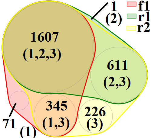
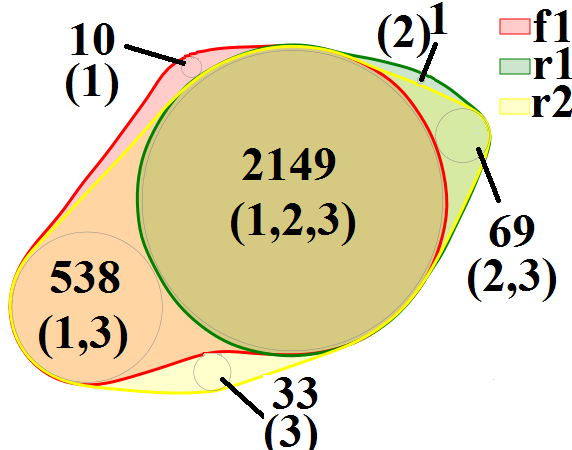
Figure 2: Relation between factor $f_{1}$ and the rules $r_{1},\ r_{2}$ for the $\mathit{NMF}_{\text{D}}$ method (left) and the $\mathit{NMF}_{\text{DE}}$ method (right).

Descriptions of obtained factors can be analysed further. For instance, supervised rules describing factor $f_{12}$, $r_{f_{12},1}\vee r_{f_{12},2}\vee r_{f_{12},3}$, where $r_{f_{12},1}=\text{heartRate}\leq 55$, $r_{f_{12},2}=\text{heartRate}\leq 59\ \wedge\ \text{RWaveDII}\leq 8.9$ and $r_{f_{12},3}=\text{heartRate}\leq 57\ \wedge\ \text{SwaveAVR}\leq 0\ \wedge\ \text{sex}=1$, obtained on the first run, on the Arrhythmia dataset describe the heart condition of $38$ individuals from which five are diagnosed as normal and $33$ as not normal. It can be seen from the rules that the heart rate of the described subjects is below normal. This condition, called bradycardia can be found in young and healthy adults (especially athletic) but there also exist a serious condition called the sick sinus syndrome. Indeed, a majority $22$ patients contained in this group are diagnosed with sinus bradycardia, one with left and four with right bundle branch block, two with ischemic changes and four with other unspecified conditions. Descriptive rules do not use target label information and are not necessarily highly homogeneous with respect to the target label. This applies to $r_{A_{dsc}}=\text{RWaveV4}\leq 17.1\ \wedge\ \text{RWaveV3}\leq 12.9\ \wedge\ \text{RWaveV2}\leq 6.7\ \wedge\ \text{RWaveV1}>24.0$, obtained on the Arrhythmia dataset, describing $70$ subjects with normal heart condition and $47$ with not normal condition.

5 Use case

Our use case example demonstrates the benefits of using the proposed methodology in a task of gene function prediction [28]. This very important task in computational biology includes developing techniques, representations and using machine learning algorithms with the goal of obtaining more accurate predictions of gene functions. The ultimate goal is to understand the role, importance and impact of genes and gene groups on the functioning and structure of the organism.

The task is being tackled using a multitude of different approaches that use data describing different aspects of organisms containing genes of interest [28]. There is also a competition aimed at developing better approaches to solve this task [1]. We focus on one sub-area that aims to develop computational models for gene function prediction using information about genomes of different organisms [28].

Our datasets contain $3475$ Clusters of Orthologous Groups (COGs) and Non-supervised Orthologous Groups (NOGs) [33]. These are groups of related genes that are known to share many functions. Gene functions are organized in a hierarchy known as Gene Ontology (GO) [2]. Each gene is assigned a number of functions (GO-terms), forming a hierarchical multi-label classification problem [34]. Our datasets contain $1047$ different gene functions.

We use three different representations for gene function prediction using genomes of $1669$ prokaryotic organisms. The first representation called the phyletic profiles [35] describes OGs by their membership in different bacterial organisms ($2731$ Boolean features). The gene neighbourhood [27] approach uses information about physical distances of OGs in genomes of different bacterial organisms ($3475$ numerical features) and the neighbourhood function profiles [23] measure the average occurrence of gene functions in a neighbourhood of each OG throughout genomes of different bacteria ($1048$ numerical features). Thus, we have three different data sources that normally constitute three different approaches for predicting gene functions using information about genomes of different organisms.

The proposed approach retains benefits such as dimensionality, sparsity reduction and non-negativity often found useful in prediction tasks where interpretation is also desirable. We will show that additionally, it can: a) achieve data fusion in an interpretable manner, b) produce representation that allows creating classifiers with better prediction of a number of gene functions compared to the original phyletic profiles approach. This is achieved by utilizing information obtained from all three data sources. This is important since such, potentially complementary approaches can be used in synergy to achieve overall, globally better predictions [35, 23] than achievable by individual components.

We created $10$ non-negative $\mathit{NMF}_{\text{MU}}$ and $\mathit{NMF}_{\text{DE}}$ representations of the phyletic profiles, containing $30$ factors. Different random initialization is used in each run. Redescriptions obtained on gene neighbourhood and neighbourhood function profiles are used as constraints to create the $\mathit{NMF}_{\text{DE}}$ representation of the phyletic profiles of the $3475$ OGs. We aim to extract knowledge that is supported by both sources, thus getting more robust knowledge. Using different types of rules allows obtaining different representations targeting different aspects of the problem.

The phyletic profiles representation is sparse containing Boolean values, thus both representations have relatively high representation errors $RE_{\mathit{NMF}_{\text{MU}}}=43.2\pm 0.05$ and $RE_{\mathit{NMF}_{\text{DE}}}=49.2\pm 0.5$, but the $\mathit{NMF}_{\text{DE}}$ has significantly higher correspondence $0.62\pm 0.04$ compared to $0.04\pm 0.01$ obtained by the $\mathit{NMF}_{\text{MU}}$. We conclude that $\mathit{NMF}_{\text{DE}}$ contains knowledge from all three data sources whereas the $\mathit{NMF}_{\text{DE}}$ contains only knowledge from phyletic profiles.

Finally, we compare the number of functions per run for which we measure improvement in the AUPRC score [4] of the Predictive Clustering tree algorithm [32] of at least $0.05$ using features obtained from $\mathit{NMF}_{\text{MU}}$ and $\mathit{NMF}_{\text{DE}}$ compared to the performance this algorithm achieved using original phyletic profiles representation (See Figure 3). Since both NMF representations contain equivalent number of features, these are directly comparable. The difference in the number of improved functions is significant according to the one-sided Wilcoxon signed-rank test [36] ($p=0.00256$).

Figure 3: Number of improved functions across $10$ different runs compared to phyletic profile approach by $\mathit{NMF}_{\text{MU}}$ (bottom) and $\mathit{NMF}_{\text{DE}}$ (top).

The proposed approach also offers potential to use described data fusion in an interpretable manner. The factor $f_{13}$ of the obtained representation using $\mathit{NMF}_{\text{DE}}$ is described with redescription $R_{f_{13}}=(q_{1,f_{13}},q_{2,f_{13}})$, where $q_{1,f_{13}}=\ \neg(10.69\leq\text{NOG091082}\leq 25.0\ \wedge\ 5.65\leq\text{COG2965}\leq 25.0\ \wedge\ 11.49\leq\text{COG0050}\leq 14.5\ \wedge\ 9.72\leq\text{COG2882}\leq 25.0\ \wedge\ 11.98\leq\text{COG1344}\leq 14.29\ \wedge\ 5.3\leq\text{COG0806}\leq 14.31)$, $q_{2,f_{13}}=0.0\leq\text{GO0046483}\leq 2.82\ \wedge\ 1.83\leq\text{GO0043228}\leq 5.88$. $R_{f_{13}}$ describes $f_{13}$ with maximum correspondence $1.0$ which means that both queries are valid for all OGs that correspond to factor $f_{13}$. From these queries, one obtains knowledge about gene and functional composition of neighbourhoods of described OGs. But, there is a third information, that of procaryotic organisms that are associated with $f_{13}$. There are in total $18$ organisms such that their corresponding attributes contribute towards $f_{13}$ with intensity larger than $0.1$. Among these, there are $4$ strains of Buchnera genus (Gram-negative bacteria that is a symbiont of aphids), $2$ strains of Bordetella (Gram-negative bacteria that can infect humans), Wigglesworthia glossinidia (Gram-negative bacteria that is endosymbiont of tsetse fly), a strain of Thermodesulfovibrio (Gram-negative bacteria that is able to reduce sulfate, thiosulfate or sulfite with a limited range of electron donors, found in hot springs), $5$ strains of Burkholderia (Gram-negative, aerobic, rod-shaped, motile bacteria), Ammonifex degensii (Gram-negative bacteria isolated from volcanic hot springs), Candidatus Desulforudis (the only example of Gram-positive bacteria, sulfate-reducing, found in groundwater at high depths), Thermovibrio ammonificans (Gram-negative, thermophilic, anaerobic, chemolithoautotrophic bacterium found in deep-sea hydrothermal vent), Thermodesulfobacterium (Gram-negative thermophilic sulfate-reducing bacteria) and Desulfurobacterium (Gram-negative, thermophilic, anaerobic, strictly autotrophic, sulphur-reducing bacterium). As we can see, the members are mostly Gram-negative bacteria or bacteria living in very high temperature equipped to process different chemical elements (mostly sulfates). This is reflected in the GO-functions that describe OGs associated to $f_{13}$, GO0043228 describes non-membrane-bounded organelle (not bounded by a lipid bilayer membrane) which is a definition of Gram-negative bacteria, whereas GO0046483 describes heterocycle metabolic process (the chemical reactions and pathways involving heterocyclic compounds, those with a cyclic molecular structure and at least two different atoms in the ring (or rings)) which corresponds to heavy chemical activity performed by many strains associated with $f_{13}$. From the query describing OG neighbourhood of OGs associated to $f_{13}$, the most understandable are COG2882 and COG1344 which are connected to cell motility (and there indeed are a number of strains like Burkholderia that are motile). COG0050 and COG0806 are connected to translation, ribosomal structure and biogenesis and COG2965 with replication, recombination and repair. The rule describing OG neighbourhood is complicated (containing logical negation), thus all OGs that have the occurrence of any of the specified OGs outside the interval, marked inside the rule, are described by this rule.

6 Related Work

Non-negative matrix factorization [24, 19] was primarily designed to enable obtaining part-based representations in different tasks, especially where non-negativity was in a problem nature. Various tasks in image and signal processing, different problems in biology, bioinformatics, pharmacy, physics, medicine etc. contain non-negative data and have been analyzed using the NMF (see [6] and references therein). It was argued that non-negativity is important in human perception and as it turns out non-negative factors are often easier to understand and interpret than factors containing negative values [25, 8]. NMF is now a mature research field with multiple developed optimization procedures, loss functions and different regularizers specifically suited for different tasks [6].

Among these regularizers, sparseness constraints [16] and ortogonality constraints [9] significantly increase overall interpretability of the NMF-produced latent factors (see [8]). The main advantage of the sparseness constraints, with respect to interpretability, is that it allows reducing the number of non-zero elements used to represent the data. Orthogonality constraint allows obtaining clear clustering assignments equivalent to that obtainable by the K-means clustering algorithm. Although very useful, orthogonality constraints are often to strict and sparseness constraints can still be hard to understand because they contain non-negative real values in the constructed matrices. Slawski et al. [30] propose the NMF approach in which the basis elements are constrained to be binary. This allows detecting overlapping clusters and it provides latent factors with binary values, which are naturally easy to understand.

7 Conclusions

This work presents a methodology for creating non-negative matrix factorization in such a way that the resulting latent factors are described by a set of input rules. The need for such methodology, which allows easy use of data fusion, is evident in various fields of science and is the addition to the continued research in interpretable non-negative factorization approaches. Two regularization terms specifically designed to model rule-based constraints are presented, each integrated in $6$ different NMF algorithms and evaluated in this manuscript. First regularization term, utilizing information about the final entity-factor assignment without using information about rule support sets explicitly, and an approach that uses explicit information about the entity membership in support sets of different rules and the input entity-factor cost matrix. This matrix expresses the descriptive constraints as the intersection size between rule support set and the entity cluster associated to the latent factor.

Experimental results performed on four different types of rules (using supervised rules, descriptive conceptual rules, subgroups and redescriptions) show that the regularizer using final entity-factor assignment mostly works better when rule clusters are predefined and associated to the latent factors. However, the approach using the cost matrix usually has lower deviation in description accuracy between factors. Algorithms using both types of regularizer create latent factors that correspond much better to the input rule set than the competing approaches. The overall representation accuracy achieved by the proposed approaches is somewhat lower compared to the regular NMF (depending on the rule-set and the input dataset). Despite the fact that the proposed approach enforces sparseness on a matrix $\mathbf{F}$, it substantially outperforms the approach that guarantees a predefined sparseness level of this matrix. The approach using entity-factor cost matrix shows large improvement when used with descriptive rules and redescriptions.

There are obvious benefits of using the proposed approach in all presented scenarios. In the unsupervised tasks, such as performing clustering with NMF, using the proposed methodology allows obtaining conceptual clusters. In the supervised tasks, the latent factors are often used as features which are further used to increase accuracy of a machine learning model. This is evident in the presented use-case where the proposed approach fusing information from multiple sources managed to improve upon an existing representation on significantly larger number of functions than regular NMF approach. In this use-case, understanding the obtained features and their connection to the target label is of utmost importance for efficient study of the underlying problem and making further research decisions. We have demonstrated the in-depth knowledge provided by the proposed approach.

References

- [1] Bio function prediction. http://www.myurl.com, 2021 (accessed April 27, 2021).
- [2] M. Ashburner, C. A. Ball, J. A. Blake, D. Botstein, H. Butler, J. M. Cherry, A. P. Davis, K. Dolinski, S. S. Dwight, J. T. Eppig, M. A. Harris, D. P. Hill, L. Issel-Tarver, A. Kasarskis, S. Lewis, J. C. Matese, J. E. Richardson, M. Ringwald, G. M. Rubin, and G. Sherlock. Gene ontology: tool for the unification of biology. the gene ontology consortium. Nat Genet, 25(1):25–29, May 2000.
- [3] M. W. Berry, M. Browne, A. N. Langville, V. P. Pauca, and R. J. Plemmons. Algorithms and applications for approximate nonnegative matrix factorization. Comput. Stat. Data Anal., 52(1):155–173, 2007.
- [4] K. Boyd, K. H. Eng, and C. D. Page. Area under the precision-recall curve: Point estimates and confidence intervals. In Machine Learning and Knowledge Discovery in Databases, pages 451–466, Berlin, Heidelberg, 2013. Springer Berlin Heidelberg.
- [5] L. Candillier and V. Lemaire. Design and analysis of the Nomao challenge - Active learning in the real-world. In ALRA Workshop, 2012.
- [6] A. Cichocki, R. Zdunek, A. H. Phan, and S.-i. Amari. Nonnegative Matrix and Tensor Factorizations: Applications to Exploratory Multi-way Data Analysis and Blind Source Separation. John Wiley & Sons, Chichester, 2009.
- [7] D. R. Cox. Note on grouping. J. Am. Stat. Assoc., 52(280):543–547, 1957.
- [8] K. Devarajan. Nonnegative matrix factorization: An analytical and interpretive tool in computational biology. PLOS Comput. Biol., 4(7):1–12, 2008.
- [9] C. Ding, T. Li, W. Peng, and H. Park. Orthogonal nonnegative matrix T-factorizations for clustering. In KDD, page 126–135, 2006.
- [10] D. Dua and C. Graff. UCI machine learning repository, 2017.
- [11] J. Fürnkranz, D. Gamberger, and N. Lavrač. Foundations of Rule Learning. Springer, 2014.
- [12] D. Gamberger, M. Mihelčić, and N. Lavrač. Multilayer clustering: A discovery experiment on country level trading data. In Discovery Science, pages 87–98, Cham, 2014. Springer International Publishing.
- [13] N. Gillis and F. Glineur. Nonnegative factorization and the maximum edge biclique problem. CORE Discussion Papers 2010059, Université catholique de Louvain, 2010.
- [14] F. E. Grubbs. Procedures for detecting outlying observations in samples. Technometrics, 11(1):1–21, 1969.
- [15] N. Hajj, Y. Rizk, and M. Awad. A subjectivity classification framework for sports articles using improved cortical algorithms. Neural Comput. Appl., 31(11):8069–8085, 2019.
- [16] P. O. Hoyer. Non-negative matrix factorization with sparseness constraints. J. Mach. Learn. Res., 5:1457–1469, 2004.
- [17] Kaggle. Abalone age classification. https://www.kaggle.com/c/predict-abalone-age/overview/description, 2018. Accessed: 2020-01-28.
- [18] W. Klösgen. Explora: A multipattern and multistrategy discovery assistant. In Advances in Knowledge Discovery and Data Mining, pages 249–271, 1996.
- [19] D. D. Lee and H. S. Seung. Learning the parts of objects by nonnegative matrix factorization. Nature, 401:788–791, 1999.
- [20] D. D. Lee and H. S. Seung. Algorithms for non-negative matrix factorization. In NIPS, page 535–541, 2000.
- [21] R. S. Michalski. A Theory and Methodology of Inductive Learning, pages 83–134. Springer, Berlin, 1983.
- [22] P. Miettinen. Matrix decomposition methods for data mining: computational complexity and algorithms. PhD thesis, University of Helsinki, Finland, 2009.
- [23] M. Mihelčić, T. Šmuc, and F. Supek. Patterns of diverse gene functions in genomic neighborhoods predict gene function and phenotype. Sci Rep 9, 9(19537):768–769, 2019.
- [24] P. Paatero and U. Tapper. Positive matrix factorization: A non-negative factor model with optimal utilization of error estimates of data values. Environmetrics, 5(2):111–126, 1994.
- [25] A. Pascual-Montano, P. Carmona-Saez, M. Chagoyen, F. Tirado, J. M. Carazo, and R. D. Pascual-Marqui. bioNMF: a versatile tool for non-negative matrix factorization in biology. BMC bioinformatics, 7(1):366, 2006.
- [26] N. Ramakrishnan, D. Kumar, B. Mishra, M. Potts, and R. F. Helm. Turning CARTwheels: An alternating algorithm for mining redescriptions. In KDD, pages 266–275, 2004.
- [27] I. B. Rogozin, K. S. Makarova, J. Murvai, E. Czabarka, Y. I. Wolf, R. L. Tatusov, L. A. Szekely, and E. V. Koonin. Connected gene neighborhoods in prokaryotic genomes. Nucleic Acids Research, 30(10):2212–2223, 05 2002.
- [28] A. Shehu, D. Barbará, and K. Molloy. A survey of computational methods for protein function prediction. In Big data analytics in genomics, pages 225–298. Springer, 2016.
- [29] M. Slawski, M. Hein, and P. Lutsik. Matrix factorization with binary components. In Advances in Neural Information Processing Systems, volume 26. Curran Associates, Inc., 2013.
- [30] M. Slawski, M. Hein, and P. Lutsik. Matrix factorization with binary components. In NIPS, page 3210–3218, 2013.
- [31] R. E. Stepp and R. S. Michalski. Conceptual clustering of structured objects: A goal-oriented approach. Artif. Intell., 28(1):43–69, 1986.
- [32] J. Struyf, S. Džeroski, H. Blockeel, and A. Clare. Hierarchical multi-classification with predictive clustering trees in functional genomics. In Portuguese Conference on Artificial Intelligence, pages 272–283. Springer, 2005.
- [33] R. L. Y. Tatusov. The cog database: a tool for genome-scale analysis of protein functions and evolution. Nucleic acids research., 28(1).
- [34] C. Vens, J. Struyf, L. Schietgat, S. Džeroski, and H. Blockeel. Decision trees for hierarchical multi-label classification. Machine learning, 73(2):185, 2008.
- [35] V. Vidulin, T. Šmuc, and F. Supek. Extensive complementarity between gene function prediction methods. Bioinformatics, 32(23):3645–3653, 2016.
- [36] F. Wilcoxon. Individual comparisons by ranking methods. In Breakthroughs in statistics, pages 196–202. Springer, 1992.