Towards a theory of hadron resonances

Abstract

In this review, we present the current state of the art of our understanding of the spectrum of excited strongly interacting particles and discuss methods that allow for a systematic and model-independent calculation of the hadron spectrum. These are lattice QCD and effective field theories. Synergies between both approaches can be exploited allowing for deeper understanding of the hadron spectrum. Results based on effective field theories and hadron-hadron scattering in lattice QCD or combinations thereof are presented and discussed. We also show that the often used Breit-Wigner parameterization is at odds with chiral symmetry and should not be used in case of strongly coupled channels.

1 Introduction: QCD and excited states

For a mathematical concept to become a dogma in describing Nature it has to be confronted with observations. In the realm of the microscopic building blocks of matter ($\sim 10^{-10}~{}\rm m$) such concepts are often far from the intuitive human experience, which is evolutionary engraved into logical concepts by dealing with everyday objects ($\sim 10^{0}~{}\rm m$). For example, the originally non-intuitive language of quantum mechanics is now an indisputable concept of any model of nuclear and particle physics. In that, one of the major breakthroughs of quantum mechanics is associated with the correct description of the pattern of excited states of atomic spectra. Going five orders of magnitude deeper ($\sim 10^{-15}~{}\rm m$) along this path, it has been discovered then that strongly interacting particles also build a complex spectrum of ground (such as proton and neutron) and excited states, so-called hadrons. It is, therefore, believed that resolving the general pattern and microscopic structure of this spectrum holds the key to the correct understanding of the strong interactions. This is the topic of hadron spectroscopy that is at the heart of the present review. Currently, the most universal language in addressing this area of research is the language of gauge field theories, which unifies the principles of special relativity and quantum mechanics incorporating local (gauge) invariance. Quantum chromodynamics (QCD) is a prime example of such a gauge theory describing the strong interaction.

Quantum chromodynamics is a truly remarkable theory passing all tests when compared to experiment for nearly five decades. Its Lagrangian can be written in a single line

$${\cal L}_{\rm QCD}=-\frac{1}{4}\,G_{\mu\nu}^{a}G^{\mu\nu,a}+\sum\limits_{f}\bar{q}_{f}(\mathrm{i}D\!\!\!/-{\cal M}_{f})q_{f}+\ldots\,,$$ (1.1)

where the ellipses denote the gauge-fixing and the $\theta$-term, which will not be considered in what follows. Here, $D_{\mu}=\partial_{\mu}-\mathrm{i}gA_{\mu}^{a}\lambda^{a}/2$ is the gauge-covariant derivative, $A_{\mu}^{a}$ ($a=1,\ldots,8$) the gluon field, $G_{\mu\nu}^{a}=\partial_{\mu}A_{\nu}^{a}-\partial_{\nu}A_{\mu}^{a}-\mathrm{i}g[A_{\mu}^{b},A_{\nu}^{c}]$ the gluon field strength tensor, $g$ is the SU(3) color gauge coupling, $q_{f}$ a quark spinor of flavor $f$ ($f=u,d,s,c,b,t$) and ${\cal M}_{f}$ is the diagonal quark matrix. The quarks come in two types, the light ($q=u,d,s$) and heavy ($Q=c,b,t$) quark flavors, where light and heavy refers to the QCD scale $\Lambda_{\rm QCD}\simeq 210$ MeV (for $N_{f}=5,\overline{\mathrm{MS}},\mu=2\,$GeV). Note that the top quark decays too quickly to participate in the strong interactions, so effectively $Q=(c,b)$. In the absence of the quark masses, $\Lambda_{\rm QCD}$ is the only dimensionful parameter in QCD that is generated by dimensional transmutation through the running of the strong coupling $\alpha_{s}=g^{2}/4\pi$. The fundamental fields of QCD, the quarks and gluons, have never been observed in isolation, which is called color confinement. They appear as constituents of the strongly interacting particles, the hadrons. This particular feature makes QCD highly non-trivial but also very interesting.

The Lagrangian of QCD allows us to define two special limits, in which the theory can be analyzed in terms of appropriately formulated effective field theories (EFTs). In the light quark ($f=u,d,s$) sector, the effective Lagrangian can be written in terms of left- ($q_{L}$) and right-handed ($q_{R}$) quark fields, such that

$${\cal L}_{\rm QCD}=\bar{q}_{L}\,\mathrm{i}D\!\!\!/\,q_{L}+\bar{q}_{R}\,\mathrm{i}D\!\!\!/\,q_{R}+{\cal O}(m_{f}/\Lambda_{\rm QCD})\,.$$ (1.2)

As can be seen, left- and right-handed quarks decouple, which is reflected in the chiral symmetry. It is explicitly broken by the finite but small quark masses $m_{f}$. Furthermore, chiral symmetry is spontaneously broken, leading to the eight pseudo-Goldstone bosons, the pions, the kaons and the eta. These are indeed the lightest hadrons, with their squared masses proportional to $m_{f}$. The pertinent EFT is chiral perturbation theory (CHPT).

Matters are very different for the heavy $c$ and $b$ quarks, where the leading order Lagrangian takes the form

$${\cal L}_{\rm QCD}=\bar{Q}_{f}\,\mathrm{i}v\cdot D\,Q_{f}+{\cal O}(\Lambda_{\rm QCD}/m_{f})\,,$$ (1.3)

with $v$ the four-velocity of the heavy quark and $Q_{f}$ denotes a quark spinor of flavor $f$ ($f=c,b$). Note that to leading order, this Lagrangian is independent of quark spin and flavor, which leads to SU(2) spin and SU(2) flavor symmetries, called HQSS and HQFS, respectively. The pertinent EFT to analyze the consequences is heavy quark effective field theory (HQEFT), which comes in different manifestations. Finally, in heavy-light systems, where heavy quarks act as matter fields coupled to the light pions, one can combine CHPT and HQEFT.

By construction, EFTs are limited to certain energy regions. A more general non-perturbative method is lattice QCD, where the Euclidean version of the theory is put on a four-dimensional space-time grid, characterized by a given lattice spacing $a$ and a finite volume, $V=L^{3}\times L_{t}$, with $L$ the spatial length ($L=Na$) and $L_{t}$ the extension in Euclidean time. Observables can be calculated by Monte Carlo simulations on the lattice. To make contact with Nature, one must consider the continuum limit $a\to 0$, the thermodynamic limit $V\to\infty$ and often has to extrapolate in the (light) quark masses down to the physical values. All this induces some systematic uncertainties, but also comes with additional value. On the one hand, varying the quark masses allows one to pin down low-energy constants of pertinent EFTs that can often only be determined approximately (or not at all) from continuum investigations and on the other hand, the volume dependence of the measured energy levels encodes information about excited states, as discussed in more detail below.

There are various reasons to consider excited states, which are the topic of this review. First, the spectrum of QCD is arguably its least understood feature. The hadron spectrum has for a long time been a playground of the constituent quark model, but we know now that this only captures certain symmetry properties of QCD, but not its full dynamics. This is evident from the questions with respect to the nature of the XYZ and other “exotic” states, where the word exotic appears between quotation marks, because this usually refers to states that can not be described within the (conventional) quark model. It is very obvious that the quark model is much too simple, as it is, e.g., it does not account for a whole class of important players in the hadron spectrum, the so-called hadronic molecules. Since the beginning of this millennium, there has been a waste activity both experimentally and theoretically to pin down the properties of these unusual (“exotic”) states, see the recent reviews [2, 3, 4, 5, 6, 7, 8, 9, 10, 11, 12, 13, 14, 15, 16, 17]. Generally, QCD permits for a whole set of bound states, which can roughly be categorized as compact states of quarks and antiquarks, states dynamically generated from hadron-hadron (or three-hadron) interactions, hybrid states made from quarks and gluons as well as glueballs, which are arguably the most exotic states QCD offers. Note, however, that in the limit of many colors $N_{c}\to\infty$, the glue sector completely decouples from the quark sector. It is also important to note that high-precision data for spectrum studies have been and will be produced with ELSA at Bonn, MAMI at Mainz, CEBAF at Jefferson Lab, the LHCb experiment at CERN, the BESIII experiment at the BEPCII, Belle-II at KEK, GlueX at Jefferson Lab and in the future with PANDA at FAIR and other labs worldwide. These data clearly pose a challenge for any theoretical approach.

In what follows, we discuss theoretical approaches that will eventually unravel the physics behind the QCD spectrum. More precisely, we only consider methods that are 1) largely model-independent, 2) can be systematically improved, and 3) allow for uncertainty estimates. If one of these conditions is not fulfilled, a given method will not be considered further, such as the Schwinger-Dyson approach, which is genuinely non-perturbative but lacks any power counting scheme. Also, we eschew models here. So that leaves us with lattice QCD (LQCD) and EFTs or combinations thereof. LQCD can get ground-states and some excited states at (almost) physical pion masses, but the most distinctive feature of excited states are decays (or the fact that the excited states have a width). Consequently, we will only consider LQCD studies of hadron-hadron scattering, that allow to extract the mass and the width of a given resonance (this also means that we will not discuss any spectrum calculations based on two-point functions). Furthermore, we will also show how the use of suitably tailored finite-volume EFTs can help in this daring endeavour.

This review is organized as follows: In Sect. 2, we define what is meant by a resonance. In Sect. 3, we discuss the basics of lattice QCD, with an emphasis on the formalisms to extract resonances. Sect. 4 consider EFTs for resonances, either as explicit fields or via some unitarization method. Sect. 5 contains the results on well separated resonances, which are only a handful. Results for the more general case of resonances with multiple decay channels (coupled channels) are collected and discussed in Sect. 6, where we also discuss the new phenomenon of the two-pole structure first observed in case of the enigmatic $\Lambda(1405)$. In section 5 and section 6 we consider publications until end of May 2022. We summarize our results in Sect. 7. As it will become clear, we still far away from a precise understanding of the hadron spectrum using the methods discussed here, but it is also remarkable to see the progress that has been made in the last decade.

2 What is a resonance?

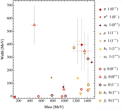
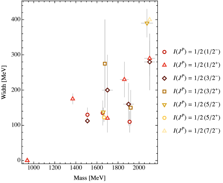
Figure 1: Spectrum of unflavored mesons (left) and light baryons (right) categorized by isospin $I$ and total angular momentum and parity $J^{P}$. Values and uncertainty regions are taken from the current review of the Particle Data Group [18].

The Particle Data Group (PDG) [18] lists around 100 excited mesonic and around 50 confirmed (4 star) baryonic states. The basic parameters of these states, the hadrons, are their mass and decay width shown for the unflavored mesons and the lightest baryons in Fig. 1. Most of these states are actually not stable, they are, broadly speaking, resonances. From the classical mechanics of a periodically driven oscillator, a resonance is characterized by two properties at the resonance frequency: a peak in the amplitude of the oscillator and a phase difference of $90^{\circ}$ between the driving force and the oscillator’s response.

This concept can be transferred to quantum mechanics, where the peak is observed in the cross section and the phase-shift between asymptotic incoming and outgoing states. For the scattering of a plane wave (wave vector $\bm{k}\in\mathds{R}^{3},~{}k:=|\bm{k}|$) with a angular momentum $\ell$ the total cross section $\sigma$ and phase-shift $\delta$ can be parameterized by the Breit-Wigner formula [19] (note that we will encounter situations where this parameterization is inadequate, see e.g. the discussion in Sect. 6.3.2)

$$\sigma(E)\propto\frac{4\pi}{k^{2}}(2\ell+1)\frac{\Gamma^{2}_{\ell}/4}{(E-E_{R})^{2}+\Gamma_{\ell}^{2}/4}\quad\text{and}\quad\tan\delta\propto-\frac{\Gamma_{\ell}}{2(E-E_{R})}\,.$$ (2.1)

This explains the name ’width’ for $\Gamma$ representing twice the distance from the peak (at $E_{R}$) to the half of the maximal value of the total cross section. The enhancement of the cross section at $E=E_{R}$ is the very origin of the term ’resonance’, see, e.g., Ref. [19]. Closely related to this is the so-called Flatté parametrization [20] which allows to address coupled-channel systems, see, e.g., Refs. [21, 22, 23] for more details and applications.

There are exemplary cases, like for instance the $\rho$-resonance, where it is to very good approximation sufficient to consider the P-wave ($\ell=1$) only. There, this quantum mechanical picture of a resonance can be carried over to quantum field theory more or less directly. However, in general the concept of resonances needs to be generalized to quantum field theories: the enhancement of the cross section can be seen as a manifestation of a new quantum (resonance) field, which couples to asymptotically stable fields and acquires, thus, a finite width through self-energy contributions Note in passing that often, an enhancement in the cross section is not seen due to the strong background or coupled channel effects. This is most clearly seen in the $P_{11}$ phase shift of pion-nucleon scattering, which is rather small in the vicinity of the Roper resonance. A prime As an example, consider a theory with two types of fields, an asymptotically stable pion (pseudo)scalar field and an unstable $\rho$ vector field. Given the coupling of the latter to two pions ($g_{\rho\pi\pi}$), the $\pi\pi$ scattering amplitude in the P-wave (see below for a formal definitions) reads

$$T_{P}(s)\propto\frac{g_{\rho\pi\pi}^{2}}{s-M_{\rho}^{2}-\Sigma(s)}\quad\text{and}\quad\Sigma(s)=\int\frac{dk\,k^{4}}{(2\pi)^{3}}\frac{g_{\rho\pi\pi}^{2}}{2E_{k}(s-4E_{k}^{2}+i\epsilon)}\,,$$ (2.2)

where $s$ denotes the total energy squared and $E_{k}=\sqrt{M_{\pi}^{2}+k^{2}}$. Note that the self-energy contribution ($\Sigma$) is divergent so that the quantities $g_{\rho\pi\pi}$ and $M_{\rho}$ need to be divergent as well since the full amplitude has to be finite. Over-subtracting the self-energy integral and introducing new subtraction constants allows then to express the scattering amplitude in terms of finite quantities only. These can be determined by fitting to experimental data as shown in Fig. 2 for the case of two subtractions.

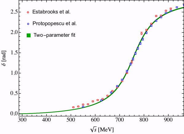
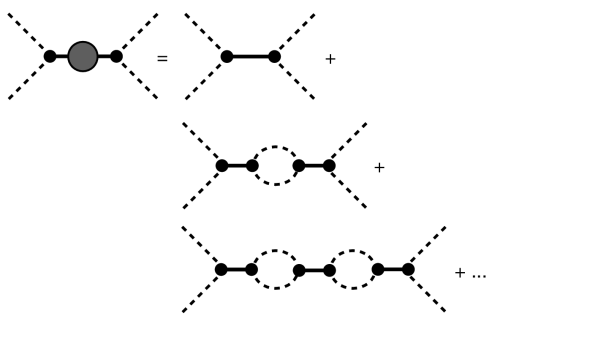
Figure 2: Left: A fit to experimental data from Refs. [24, 25] using twice subtracted self-energy of the $\rho$ field, see Eq. (2.2). Green band represents 1-sigma statistical uncertainty region of the two-parameter fit, respectively. Right: Diagrammatic representation of the $\rho$ resonance in $\pi\pi$ scattering via a bare state (full line) and self-energy due to coupling to asymptotically stable pion fields (dashed line).

We note further that often an enhancement in the cross section is not seen due to the strong background or coupled-channel effects. This is most clearly seen in the $P_{11}$ phase shift of pion-nucleon scattering, which is rather small in the vicinity of the Roper resonance. Or as it is often stated: “Not every bump is a resonance and not every resonance is a bump”, see, e.g., the discussion in Ref. [26]

The introduction of auxiliary (resonance) fields is a useful tool in many applications of hadron physics, see, e.g., Refs. [27, 28, 29] for recent applications to multihadron systems. However, there are many examples, such as $f_{0}(500)$ or $\Lambda(1405)$, where such a representation is not sufficient. The most universal and modern approach to resonances deals directly with scattering amplitudes. In that, the so-called $S$-matrix – originally introduced by Heisenberg [30] – relates the asymptotic in- (three-momenta $\bm{p}_{1},...,\bm{p}_{m}$) and outgoing (three-momenta $\bm{p}^{\prime}_{1},...,\bm{p}^{\prime}_{n}$) states as

$$\langle\bm{p}^{\prime}_{1},...,\bm{p}^{\prime}_{n}|S|\bm{p}_{1},...,\bm{p}_{m}\rangle=\langle\bm{p}^{\prime}_{1},...,\bm{p}^{\prime}_{n}|(\mathds{1}+\mathrm{i}T)|\bm{p}_{1},...,\bm{p}_{m}\rangle\,,$$ (2.3)

which defines the so-called $T$-matrix. The $S$-matrix obeys crossing symmetry, i.e., the $S$-matrix element for a $n\to m$ transition can be converted analytically to the element describing $n+1\to m-1$ transitions etc.. Furthermore, and crucial for the matter of the present review is the principle of analyticity. It is rooted in the requirement of causality [31, 32] for physical processes and states that physical $S$-matrix elements are boundary values to an analytic functions in all inner products of all involved momenta ($\bm{p}^{(\prime)}_{i}\bm{p}^{(\prime)}_{j}$) or in closely related generalized Mandelstam variables, promoted to their complex values. In that, the choice of variables is not unique but the number of independent ones is fixed. First, since all in-/outgoing states are on the respective mass shell $\left(p^{(\prime)}_{i}{}^{2}=m^{(\prime)2}_{i}\right)$ only $3(m+n)$ combinations can be independent. Furthermore, energy-momentum conservation and choice of the reference frame constrain the number of independent invariants to $3(m+n)-4-6$, see Ref. [33] for more details. Finally, following the latter reference the $S$-matrix can be expressed as

$$S=\sum_{i}{}_{\rm in}|i\rangle\langle i|_{\rm out}\quad\text{for}\quad{}_{\rm out}\langle i|j\rangle_{\rm in}=\delta_{ij}\quad\text{and}\quad\sum_{i}{}_{\rm in}|i\rangle\langle i|_{\rm in}=\sum_{j}{}_{\rm out}|j\rangle\langle j|_{\rm out}=\mathds{1}\,,$$ (2.4)

i.e., using complete and orthonormal set of physical states. This obviously leads to the unitarity of the $S$-matrix, $SS^{\dagger}=S^{\dagger}S=\mathds{1}$, which physically ensures probability conservation [30]. It is notable that the number of physical states depends on the energy of the system. For a generic two-body systems with identical particles of mass $\mu$ (equivalently for other cases) and total energy squared $s$ this yields schematically that

$$\vbox{\hbox{\includegraphics[width=170.71652pt,trim=0.0pt 512.1496pt 455.24408pt 0.0pt,clip]{S-unitarity.pdf}}}~{}\begin{aligned} (N)^{2}\leq s/\mu^{2}<(N+1)^{2}\,.\end{aligned}$$ (2.5)

Overall, unitarity, analyticity and crossing symmetry are the main principles of $S$-matrix theory going beyond expansion in Feynman diagrams. The pertinent matrix elements are expected to encode all information about the dynamics of the system including the properties of the resonances as will be discussed below.

Unitarity of the $S$-matrix implies for the $T$-matrix that $(T-T^{\dagger})=\mathrm{i}T^{\dagger}T$, leading for a general $n\to n$ transition to the following condition on the matrix elements and invariant matrix element

$${\mathcal{M}(\{p\}\to\{p^{\prime}\})=(2\pi)^{4}\delta^{(4)}\left(\sum_{i=1}^{n}p_{i}-p_{i}^{\prime}\right)\langle\bm{p}_{1}^{\prime}\bm{p}_{2}^{\prime}|T|\bm{p}_{1}\bm{p}_{2}\rangle}$$ (2.6)

with

$$\langle\bm{p}^{\prime}_{1},...,\bm{p}^{\prime}_{n}|(T-T^{\dagger})|\bm{p}_{1},...,\bm{p}_{n}\rangle =\mathrm{i}\int\prod_{i=1}^{N}\frac{\mathrm{d}^{4}k_{i}}{(2\pi)^{4}}\,(2\pi)\delta^{+}(k_{i}^{2}-m^{2})\langle\bm{p}^{\prime}_{1},...,\bm{p}^{\prime}_{n}|T^{\dagger}|\{\bm{k}\}\rangle\,,\langle\{\bm{k}\}|T|\bm{p}_{1},...,\bm{p}_{n}\rangle\,,$$ (2.7)

$$\mathcal{M}(\{p\}\to\{p^{\prime}\})-\mathcal{M}^{*}(\{p^{\prime}\}\to\{p\}) =\mathrm{i}\int\prod_{i=1}^{N}\frac{\mathrm{d}^{4}k_{i}}{(2\pi)^{4}}\,(2\pi)\delta^{+}(k_{i}^{2}-m^{2})\,(2\pi)^{4}\delta^{(4)}\left(P-\sum_{i=1}^{N}\,k_{i}\right)\mathcal{M^{*}}(\{p^{\prime}\}\to\{k\})\mathcal{M}(\{p\}\to\{k\})\,,$$

where $\delta^{+}(k_{i}^{2}-m^{2})$ selects the positive energy solution, $P$ denotes the total four momentum of the system, and the size of the complete set of intermediate states ($N$) depends on the total energy of the system, see Eq. (2.5). The integration over intermediate momenta on the right-hand-side of the latter equation leads to another crucial and beautiful implication for the structure of the $S$-matrix.

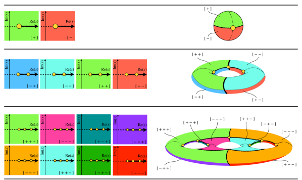
Figure 3: Representation of the Riemann surface for one (top row) and two (middle row) and three (bottom row) open two-body thresholds. The value of $|s|=\infty$ is put for simplicity on the poles of the sphere and rim of the tori, respectively. Riemann Sheets are denoted by a sequence $[\pm\pm...]$ as discussed in the main text. Yellow dots depict the position of the branch points.

As an example, consider a simple case of $2\to 2$ scattering of identical particles, where by limitations due to total energy of the system or some quantum numbers only two-body intermediate states are allowed. Then, for the invariant matrix element $\mathcal{M}(p_{1},p_{2}\to p_{1}^{\prime},p_{2}^{\prime})=(2\pi)^{4}\delta^{(4)}(p_{1}+p_{2}-p_{1}^{\prime}-p_{2}^{\prime})\langle\bm{p}_{1}^{\prime}\bm{p}_{2}^{\prime}|T|\bm{p}_{1}\bm{p}_{2}\rangle$ and the corresponding partial wave expansion $\mathcal{M}_{\ell}(s)=1/(64\pi)\int_{-1}^{+1}dz\mathcal{M}(s,z)P_{\ell}(z)$ the unitarity relation simply implies that

$$\text{Im}\,\mathcal{M}_{\ell}^{-1}(s)=-\frac{2q(s)}{\sqrt{s}}\theta\left(\sqrt{s}-2m\right)\qquad\text{with}\quad q(s)=\sqrt{\frac{s}{4}-m^{2}}\,,$$ (2.8)

where $m$ denotes the mass of the involved field. This implies that a two-body system is described by a set of partial wave amplitudes of the form

$$\mathcal{M}_{\ell}(s)=\frac{\sqrt{s}}{2}\frac{1}{K_{\ell}^{-1}(s)-\mathrm{i}q}\,,$$ (2.9)

for some real function $K_{\ell}(s)$ referred to as the K-matrix and related to observable two-particle phase-shifts as $K^{-1}_{\ell}(s)=q(s)\cot\delta_{\ell}$. The key point is that due to multi-valuedness of the square root function, also the partial wave amplitude is in general multivalued. The energy at which the multi-valuedness first occurs (lowest energy at which participating states first go on-shell) is referred to as the branch point. Thus, the domain of the function $T_{\ell}(s)$ is extended from $s\in\mathds{C}$ to $s\in\mathds{C}\times\mathds{C}$, representing a complex manifold referred to as the Riemann surface consisting of two Riemann sheets, each covering $\mathds{C}$. Generalizing this, a partial wave amplitude covering $m$ possible intermediate two-body channels is a complex-valued function on a $2^{m}$ sheeted Riemann surface. Three examples of a one-, two- and three-channel problem are shown in Fig. 3. There, individual sheets are shown together with a diffeomorphic mapping of those to a three-dimensional manifolds of gender zero, one and three, respectively. The latter mapping demonstrates clearly how all $2^{m}$ Riemann sheets are connected to one-another. Any measured (experimentally or as a result of a numerical lattice calculation) values are located on the real energy-axis of the so-called physical sheet, see the green-shaded sheet denoted by $[+\ldots+]$ referring to ${\rm Sgn}(\text{Im}\,(q(s)))$ in each two-body channel. Generalizing this notation, we denote all sheets by the same type of sequence, see, e.g., Refs. [34, 35]. Specifically, the unphysical sheet connected to the physical one between the first and second threshold is denoted by $[-+\ldots+]$, the one connected to the physical sheet between the second and third threshold by $[--+\ldots+]$ etc. .

Coming back to the matter of resonances, we recall that the $S$-matrix (and with it also the scattering amplitude $T$) is a holomorphic function – smooth in a neighborhood of any complex-valued point – with respect to the discussed complex-valued (e.g., generalized Mandelstam) variables. The only allowed exception to this is the presence of bound states on the real axis below the production threshold. Furthermore, and as we have seen with explicit fields, excited hadrons or resonances can be associated with poles in the complex plane. Thus, these poles can only be located on the unphysical sheets of the analytically continued $S$-matrix. Typically, only closest to the physical axis located sheets ($[-+\ldots+]$, $[--+\ldots+]$, etc.) are searched for the resonances, as it is assumed that their influence on the physical processes is anti-proportional to the direct (perpendicular to $\text{Re}\,s$) distance to the real energy axis. Of course, in general more complex situations occur and poles on remote Riemann sheets can be of importance as well, see, e.g., Refs. [35, 36]. So far we have discussed examples with two-body states only. However, when more particles are present either in the in/out or intermediate states, the picture remains with the exception that if, e.g., two particles subsystems interact resonantly additional branch cuts occur in the complex $s$-plane [37]. An example, of such a case is the $3\pi$ system with $I^{G}(J^{PC})=1^{-}(1^{++})$ quantum numbers, where two of three pions form a resonant subsystem corresponding to the $\rho$-meson, see, e.g., Refs. [38, 39]. This is depicted in the left panel of Fig. 4.

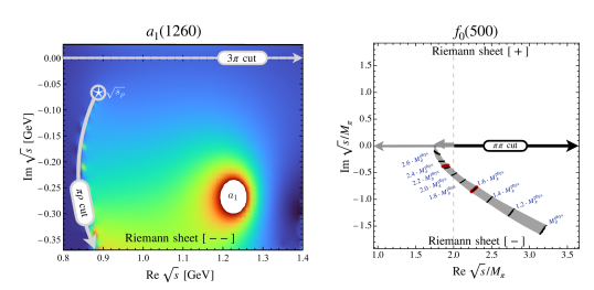
Figure 4: Left: Unphysical $[--]$ Riemann sheet of the $3\pi$ system including resonance pole of the $a_{1}(1260)$ state. Double cut structure arises from three-pions being on-shell as well as two pions forming a $\rho$-resonance. Figure adopted from Ref. [38]. Right: Pole movement of the $f_{0}(500)$-resonance as a function of the pion mass in terms of the physical pion mass ($M_{\pi}^{\rm phys}$). Black dots and gray band represent pole position resampled with respect to the lattice QCD calculations at the unphysical pion masses [40, 41, 42, 43].

In summary, the modern approach to resonances utilizes the concept of the $S$-matrix. Induced by the requirement of unitarity (probability conservation), analyticity (causality of physical processes) and crossing symmetry, it is fixed on the real energy-axis by experimental or more recently lattice QCD results. When fixed, it is believed to contain all information about the exited states of hadrons. Specifically, any state is described by a complex-valued position of its pole on a given Riemann sheet. Such parameters are universal, i.e., they do not depend on the choice of a particular transition. Coupling to specific initial and final states is encoded in the residuum of the pole of a scattering amplitude to such states. This interpretation naturally unites the concept of bound states (poles on the real energy-axis on the physical Riemann sheet below production threshold), virtual states (poles on the real energy-axis on the unphysical Riemann sheets) and resonances (complex energy poles on the unphysical Riemann sheets). Interestingly, the transition between different regimes can be tested using lattice QCD calculations at different (unphysical) quark masses. The prominent example in this regard is the long-debated scalar isoscalar mesonic $f_{0}(500)$, see the recent review [44]. The pion mass dependence of the $f_{0}(500)$ pole has been studied extensively with methods based on unitarity and chiral perturbation theory, see, e.g., Refs. [45, 46, 41]. The results of a recent study backed by lattice QCD at unphysical pion masses [40, 41, 42, 43] are shown in the right panel of Fig. 4.

3 Theoretical methods I: Lattice QCD

In this section we introduce Lattice QCD, the formulation of QCD in Euclidean space-time regularized by confining the theory to a finite volume on a discrete hyper-cubic lattice. The main focus of this section is to familiarize the reader with the relevant concepts but also to enable the reader to understand the systematics of this method. More details can be found in textbooks on the topic of lattice field theory.

3.1 QCD on a lattice

We recall the renormalizable QCD Lagrangian that conserves parity and is invariant under time reversal, Eq. (1.1), for a single quark flavor $q$

$$\mathcal{L}=-\frac{1}{4}(G_{\mu\nu}^{a})^{2}+\bar{q}(\mathrm{i}\gamma^{\mu}D_{\mu}-m_{q})q\,.$$ (3.1)

Here, $\bar{q}=q^{\dagger}\gamma_{0}$ and

$$G_{\mu\nu}^{a}=\partial_{\mu}A_{\nu}^{a}-\partial_{\nu}A_{\mu}^{a}+gf^{abc}A_{\mu}^{b}A_{\nu}^{c}$$ (3.2)

is the field strength tensor. The structure constants of SU$(3)$ are denoted by $f^{abc}$, while $g$ is the bare gauge coupling constant and $m_{q}$ is the bare quark mass parameter. The the vector potential is denoted by $A$. This theory needs regularisation and renormalization.

For the lattice regularisation we start in Euclidean space-time, i.e., after analytically continuing to purely imaginary times $t\to-\mathrm{i}t$. The Euclidean action then reads

$$S\ =\ \int\mathrm{d}^{4}x\left[\frac{1}{4}(G_{\mu\nu}^{a})^{2}+\bar{q}(\gamma_{\mu}D_{\mu}+m_{q})q\right]\,,$$ (3.3)

with Euclidean $\gamma$-matrices satisfying

$$\{\gamma_{\mu},\ \gamma_{\nu}\}\ =\ 2\,\delta_{\mu\nu}\,.$$ (3.4)

The Euclidean partition function $\mathcal{Z}$ is then given by

$$\mathcal{Z}\ =\ \int\mathcal{D}\bar{q}\ \mathcal{D}q\ \mathcal{D}A\mathrm{e}^{-S}\,,$$ (3.5)

with the Euclidean action being real and bounded from below. This allows one to interpret the exponential factor as a probability weight and enables Monte Carlo integration methods to be applied.

In order to make such a Monte Carlo approach work in practice, the system is confined into a finite volume with spatial extents $a_{s}L_{k}\,,\ k=1,2,3$, and temporal extent $a_{t}L_{4}$. This hypercube is then discretized with lattice spacings $a_{s}$ in spatial and $a_{t}$ in temporal directions. Denoting here and in the following Euclidean four-vectors by $\vec{x}$, the set of lattice sites can be written as

$$\Lambda\ =\ \{\vec{n}:\quad n_{\mu}=0,1,...,L_{\mu}-1\,;\mu=1,2,3,4\}\,.$$ (3.6)

In doing so the theory is regularized both in the infrared by the finite volume and the ultraviolet by the discretization. Typically one chooses $L_{k}=L,k=1,2,3$ and $L_{4}=T$ in lattice simulations, a notation that we will also adopt where possible.

Furthermore, the fermionic fields $\bar{q},q$ are defined only on the lattice sites $\bar{q}(\vec{n})\,,\ q(\vec{n})$ and the integral over the volume becomes a sum

$$\int\mathrm{d}^{4}x\quad\to\quad\frac{1}{L_{1}L_{2}L_{3}L_{4}}\sum_{\vec{n}\in\Lambda}\,,$$ (3.7)

and the functional integrals for the Grassmann valued fermionic fields read

$$\mathcal{D}\bar{q}\ \mathcal{D}q\quad\to\quad\prod_{\vec{n}\in\Lambda}\,\mathrm{d}\bar{q}(\vec{n})\ \mathrm{d}q(\vec{n})\,.$$ (3.8)

The lattice gauge field is represented by SU$(3)$-valued fields $U_{\mu}(\vec{n})\equiv U_{\vec{n},\mu}$ in the fundamental representation, which connect lattice sites $\vec{n}$ and $\vec{n}+\hat{\mu}$, where $\hat{\mu}$ is the unit vector in direction $\mu$. This allows one to also define the functional integral over the gauge fields on the lattice by the transition

$$\int\ \mathcal{D}A\quad\to\quad\int\prod_{\vec{n}\in\Lambda,\mu}\mathrm{d}U_{\vec{n},\mu}\,,$$ (3.9)

denoting the invariant Haar measure [47] by $\mathrm{d}U$. The parallel transports $U_{\vec{n},\mu}$ are related to the gauge potential $A_{\mu}$ via

$$U_{\vec{n},\mu}\ =\ \mathrm{e}^{\mathrm{i}gaA_{\mu}(\vec{n}+\hat{\mu}/2)}\,.$$

For the gauge fields usually periodic boundary conditions are used, though also open boundary conditions are used to mitigate topological freezing [48]. For the fermionic fields boundary conditions are in general implemented by a phase factor

$$q(\vec{n}+L_{\mu}\hat{\mu})=\mathrm{e}^{\mathrm{i}\theta_{\mu}}q(\vec{n})\,,$$ (3.10)

with angles $\theta_{\mu}\in[0,2\pi[\,,\ \mu=1,2,3,4$.

3.2 Lattice actions

It remains to discretize the different elements in the Euclidean action, while maintaining gauge invariance. For convenience, we assume $a_{s}=a_{t}=a$ here for the moment. The pure gauge part can be written in terms of the $U$-fields as follows

$$S_{g}\ =\ -\frac{\beta}{3}\sum_{\vec{n}}\left(b_{0}\sum_{1\leq\mu<\nu}\mathrm{Re}\,\mathrm{Tr}\,\left(U^{1\times 1}_{\vec{n},\mu,\nu}\right)+b_{1}\sum_{\mu\neq\nu}\mathrm{Re}\,\mathrm{Tr}\,\left(U^{1\times 2}_{\vec{n},\mu\nu}\right)\right)\,.$$ (3.11)

Here, the bare inverse coupling $\beta=6/g^{2}$, while $U^{1\times 1}_{\vec{n},\mu,\nu}$ represents the so called plaquette loop

$$U^{1\times 1}_{\vec{n},\mu,\nu}\ =\ U_{\vec{n},\mu}^{~{}}U_{\vec{n}+\hat{\mu},\nu}^{~{}}U_{\vec{n}+\hat{\nu},\mu}^{\dagger}U_{\vec{n},\nu}^{\dagger}\,,$$ (3.12)

which corresponds to the smallest closed loop in the $\mu-\nu$ plane on a lattice. $U^{1\times 2}_{\vec{n},\mu\nu}$ is defined analogously as the Wilson loop in the $\mu-\nu$ plane with edge lengths $1$ and $2$ in direction $\mu$ and $\nu$, respectively.

The parameter choice $b_{0}=1,b_{1}=0$ corresponds to the original Wilson gauge action [49]. Up to corrections of order $a^{2}$ this action reproduces the continuum gauge action. Improved choices for $b_{0},b_{1}$ have been introduced for instance in Refs. [50, 51] on which most modern lattice QCD simulations are based on.

For the discretization of the Dirac operator $D_{\mu}$ there are many different choices possible, all differing by lattice artefacts and symmetry properties. The most prominent ones are Wilson’s discretization [49], the so-called staggered or Kogut-Susskind discretization [52, 53], the overlap [54, 55] and domain-wall discretizations [56, 57]. The latter two allow for exact chiral symmetry on the lattice [58].

For $a_{s}\neq a_{t}$ the gauge action needs to be split into one term involving only spatial loops and a second one involving space-time loops, which requires the introduction of inverse couplings $\beta_{s}$ and $\beta_{t}$. $\beta$ (and $\beta_{t}$ and $\beta_{s}$) are related to the lattice spacing value(s) via the QCD $\beta$-function. For details we refer to Refs. [59].

Most relevant for this review are discretizations based on the Wilson discretization. The corresponding part of the action for a doublet of mass-degenerate Wilson type quarks $q$ – which we interpret as a vector in space, time, spin and colour – reads

$$S_{q}=\bar{q}\left[D_{W}(U)+m_{0}+\mathrm{i}\mu_{q}\gamma_{5}\tau^{3}+\frac{\mathrm{i}}{4}c_{\mathrm{SW}}\sigma^{\mu\nu}\mathcal{F}^{\mu\nu}(U)\right]q\,,$$ (3.13)

where $\mu_{q}$ is the bare twisted mass parameter and $\tau^{3}$ is the third Pauli matrix acting in flavor space. Furthermore, $D_{\mathrm{W}}$ represents the massless Wilson Dirac operator

$$D_{\mathrm{W}}(U)=\frac{1}{2}\left[\gamma_{\mu}(\nabla_{\mu}^{~{}}+\nabla_{\mu}^{\star})-ar\nabla_{\mu}^{\star}\nabla_{\mu}^{~{}}\right]\,,$$ (3.14)

with $\nabla_{\mu}$ and $\nabla_{\mu}^{\star}$ the gauge covariant forward and backward difference operators given by

$$\nabla_{\mu}q(\vec{n})\ =\ U_{\vec{n},\mu}^{~{}}\,q(\vec{n}+\hat{\mu})-q(\vec{n})\,,\qquad\nabla_{\mu}^{\star}q(\vec{n})\ =\ q(\vec{n})-U_{\vec{n}-\hat{\mu},\mu}^{\dagger}\,q(\vec{n}-\hat{\mu})\,,$$ (3.15)

respectively. The Wilson parameter is usually set to $r=1$ and $m_{0}$ is the bare Wilson mass parameter. Finally, the so-called Sheikoleslami-Wohlert improvement coefficient [60] is denoted by $c_{\mathrm{sw}}$ with $\mathcal{F}^{\mu\nu}$ being a discretization of the field strength tensor, see for instance Ref. [61].

With $\mu_{q}=0$ and $c_{\mathrm{SW}}=0$ the action eq. 3.13 corresponds to Wilson’s discretization. With only $\mu_{q}=0$ we have so-called clover improved lattice fermions [62], which are with appropriate tuning of the value of $c_{\mathrm{SW}}$ $\mathcal{O}(a)$ improved, i.e., lattice artefacts are coming at $a^{2}$, while the pure Wilson discretization has artefacts proportional to $a$. With $\mu_{q}\neq 0$ the discretization is called Wilson clover twisted mass fermions [63, 64], which has the property of automatic $\mathcal{O}(a)$ improvement [65] independent of the choice for $c_{\mathrm{SW}}$ for particular choices of $m_{0}$ and $\mu_{q}$ (so-called maximal twist).

The different Wilson type discretizations come with their own advantages and disadvantages. This is to a large extend a technical issue which for the scope of the present review merely affects the size of lattice artefacts. However, also the symmetry properties of the actions differ, most notably for twisted mass fermions where isopsin and parity symmetries are broken at the level of $a^{2}$ lattice artefacts [65]. Moreover, the renormalization patterns are different: for instance can the pion decay constant $f_{\pi}$ be determined without the need of multiplicative renormalization in the twisted mass formulation, while with Wilson and Wilson clover fermions this is not the case.

Further diversity in the lattice discretization comes by the usage of gauge field smearing in the covariant derivative. Smearing is used to reduce ultraviolet fluctuations in the gauge field and, thus, lattice artefacts in observables. Typically so-called stout smearing [66] or HEX smearing [67] is used.

Finally, lattice QCD simulations are performed with different numbers of dynamical quark flavors: $N_{f}=2$, $N_{f}=2+1$ and $N_{f}=2+1+1$ for simulations with mass degenerate up and down quarks plus strange or strange and charm quarks. The not active quark flavors are in turn assumed to be infinitely heavy and, therefore, decoupled. The number of flavors is particularly important, in the context of this review, to understand which decay channels are open in a lattice calculation. For example, if strange quarks are not dynamically simulated, a sufficiently heavy resonance made from up and down quarks cannot decay into two kaons.

Note that in order to prove positivity of the transfer matrix for Wilson’s discretization anti-periodic boundary conditions in time for the fermionic fields are required [68]. This, in turn, is a prerequisite for the so-called Osterwalder-Schrader reflection positivity, which is mandatory for the analytical continuation from Euclidean to Minkowski space [69, 70].

3.2.1 Valence versus Sea Quarks

Lattice simulations can involve more than the lattice action used for the Monte Carlo simulations: valence quarks can be added using a different discretization than the one used for the sea quarks. This is called a mixed action approach. It is even possible to add valence quarks that are not present in the sea, in case of which one speaks about partially quenched simulations.

Working in a mixed action situation can be useful if properties of the valence quarks are required or desirable, which are too resource demanding for the full Monte Carlo simulation. Such properties can be for instance additional symmetries or reduced lattice artefacts. It requires a matching procedure of sea and valence actions: typically one computes one or several hadron masses with only sea and with only valence quarks and tunes the valence parameters until sea and valence hadrons agree (within statistical uncertainties). Typical examples are valence quarks with exact chiral symmetry on top of a sea action with the Wilson or staggered fermion discretization.

A partially quenched configuration is typically used to include strange or charm quarks in the valence sector that are not present in a $N_{f}=2$ or $N_{f}=2+1$ sea action. This allows one for instance to study $K$-, $D$- and $D_{s}$-mesons in lattice QCD simulations with $N_{f}=2$ dynamical quarks. It is important to realise that valence quarks not present in the sea cannot annihilate. Still in some cases with saturated quantum numbers, such simplified calculations may reflect the physical system, e.g., the recent calculation of $K^{-}K^{-}K^{-}$ scattering [71].

3.2.2 Heavy Quarks

As discussed in the introduction, heavy and light quarks are usually treated differently, which is also the case on the lattice. The main reason is the following: every quark flavor comes with its quark mass parameter $m_{q}$. In a lattice simulations the relevant quantity is actually the quark mass in lattice units, i.e., $am_{q}$. In order for the discretization to be meaningful one would argue that $am_{q}\ll 1$ should be fulfilled. The lattice spacing is typically around $0.1\ \mathrm{fm}$. Thus, for the charm quark $am_{c}\approx 0.8$, but for the bottom quark $am_{b}>2$. Even with $a\sim 0.05\ \mathrm{fm}$, which is nowadays used in some simulations, $am_{b}$ is above the cutoff. On the other hand, dynamical effects of quarks become less and less important with increasing mass.

These are the main reasons why lattice simulations should be performed including at least up and down and strange quarks dynamically. Since $N_{f}=2$ simulations are easier to perform and require less resources, they were explored before simulating with $N_{f}=2+1$ dynamical flavors, and the corresponding simulations are still being analysed. For the charm quark it is not entirely clear whether or not sea effects can be neglected. The main reason for not including it in the dynamical simulation are potentially large lattice artefacts of $\mathcal{O}(am_{c})$. However, it is certain that the bottom quark will not be included as a dynamical degree of freedom in lattice simulations in the near future.

We remark here that simulations with Wilson twisted mass quarks at maximal twist can only be performed either in- or excluding a strange/charm doublet. However, so-called automatic $\mathcal{O}(a)$ improvement means that effects of $\mathcal{O}(am_{c})$ are absent and the relevant lattice artefacts start at $\mathcal{O}((am_{c})^{2})$.

The question remains of how to treat charm and bottom quarks in the valence sector when studying heavy-light mesons, where a charm or bottom quark is combined with one of the three light quarks, or when one is interested in quarkonia. There are two strategies:

• Treat heavy quarks relativistically. While this appears to become more or less the standard for the charm quark, the bottom requires either an improvement program, see Ref. [72]. Or clever strategies need to be devised [73]. In the latter case the idea is to construct suitable ratios with a well defined static limit. Computing these ratios in the charm quark mass region and smoothly interpolating to the static limit allows one to compute $B$-physics observables without being compromised by large systematic uncertainties stemming from $am_{b}>1$.

• Treat heavy quarks in an effective theory. The choices are heavy quark effective theory with expansion parameter $1/m_{q}$ or non-relativistic QCD with the expansion parameter $v$ denoting the modulus of the four velocity of the heavy quark. HQEFT is appropriate for heavy-light systems, while NRQCD is more appropriate for quarkonia.

In both cases, the zeroth-order Lagrangian reads in Euclidean space-time

$$\mathcal{L}_{0}=q_{+}^{\dagger}(-D_{0}+m_{q})q_{+}\,,$$ (3.16)

with fields projected to quark (antiquark) fields $q_{\pm}=(1\pm\gamma_{0})q/2$. In this static limit the propagator is just a straight Wilson line. The Lagrangian eq. 3.16 can be systematically improved to include higher order corrections in the respective expansion parameter. We remark here that in section 6, where we compile recent results, the lattice results have been all obtained by treating the charm quark relativistically.

3.3 Resonances in a finite volume

In the previous subsection we discussed that Monte Carlo simulations are enabled by working in Euclidean space-time. This has certain consequences for the observables, which can be investigated, even if Osterwalder-Schrader reflection positivity holds. Generally speaking, observables connected to real time turn out to be problematic, such as scattering amplitudes, as was pointed out long ago by Maiani and Testa [74].

3.3.1 Lüscher’s method

A way out was found by Lüscher, who devised a method based on the works [75, 76] now coined as Lüscher method [77, 78]. Generally speaking, the method is based on the observation that the energy spectrum of the lattice Hamiltonian depends on the volume. And this dependence on the volume encodes information on the scattering properties, because with decreasing volume the interaction probability increases.

In practice the situation is more complicated because there are different contributions to finite-volume induced energy shifts. In particular, there are contributions which are for large enough $L$ exponentially suppressed and of the form $\exp(-M_{\pi}\cdot L)$ [79, 80]. These exponential finite-volume effects compete with those only power suppressed in $1/L$, which are the ones related to infinite-volume scattering properties.

Lüscher’s method is by now well established and applicable for the case that the exponential finite-volume effects are negligible compared to the power suppressed ones. A detailed summary of the two particle formalism can be found in the recent review articles [81, 82, 83]. Most recently, the Lüscher method has been generalized also to the three-body case [84, 85, 86, 87, 88, 89, 90, 91, 92, 93, 94, 71, 95, 96, 97, 98, 99, 100, 101, 102, 38, 103, 104, 105, 106], see also recent reviews [107, 108].

Instead of writing here the most general formalism, we will focus on the particular case of scattering of two equal mass mesons below inelastic threshold. The observable to be determined from lattice data are phase-shifts $\delta_{\ell}(k^{2})$ for partial wave $\ell$ as a function of the squared scattering momentum $k^{2}$. Lüscher’s method is formulated by means of the following finite-volume quantisation condition

$$\det\left[\mathcal{M}_{\ell m,\ell^{\prime}m^{\prime}}(k^{2},L,\bm{p}_{\mathrm{cm}})-\delta_{\ell\ell^{\prime}}\delta_{mm^{\prime}}\,\cot\left(\delta_{\ell}(k^{2})\right)\right]\ =\ 0\,,$$ (3.17)

where the determinant acts in angular momentum space. The lattice input to this formula is encoded in the analytically known matrix valued function $\mathcal{M}_{\ell m,\ell^{\prime}m^{\prime}}(k^{2},L,\bm{p}_{\mathrm{cm}})$, which contains the famous Lüscher $\mathcal{Z}$-function and which is in general not diagonal in angular momentum. $\mathcal{M}$ depends on the squared scattering momentum $k^{2}$ (or equivalently the scattering energy), the lattice extend $L$ and the total momentum of the two particle system in the centre-of-mass frame $\bm{p}_{\mathrm{cm}}$, which is quantized due to finite volume

$$\bm{p}_{\mathrm{cm}}=\frac{2\pi}{L}\cdot\bm{d}\,,\quad\bm{d}\in\mathbb{Z}^{3}\,.$$ (3.18)

Given the (lattice) energy level of the two body systems $E_{\mathrm{CM}}$ in the centre-of-mass frame, the scattering momentum is then given by

$$k^{2}\ =\ \frac{E_{\mathrm{CM}}^{2}}{4}-M^{2}\,,$$ (3.19)

where $M$ is the infinite-volume single meson mass value. Momentum sectors are usually classified by $\lvert\bm{d}\rvert^{2}$. The set of equivalent momenta is denoted as

$$\{\bm{d}\}\equiv\{\bm{z}\in\mathbb{Z}^{3}\,,\quad{\bm{z}}^{2}=\bm{d}^{2}\}\,.$$ (3.20)

It becomes apparent that for each set of values $\{k^{2},L,\lvert\bm{d}\rvert^{2}\}$ one value of $\delta_{l}$ can be determined. Therefore, in order to determine the phase-shift for a dense as possible set of scattering momenta, significant effort was put into generalising Lüscher’s formalism for different moving frames [109, 110, 111]. For two particle system the formalism is spelled out for general spin in Ref. [112].

In principle, the matrix $\mathcal{M}$ is dense, because angular momentum is no longer a good quantum number even for the zero-momentum case, because the continuum rotation groups is broken down to the octrahedal or cubic group. All infinite-volume angular momenta fall, therefore, in one of the ten irreducible representations $\Gamma$ of the octahedral group. When considering also non-zero total momentum of the multi-particle system, symmetries are further reduced to so-called little groups (or stabilisers) with corresponding irreducible representations. Every lattice irreducible representation contains an infinite tower of continuum angular momenta, but not all.

Still, even this reduced amount of symmetry helps in simplifying eq. 3.17: when operators are projected into the lattice irreducible representations $\Gamma$ (so-called subduction), the matrix $\mathcal{M}$ becomes block diagonal significantly simplifying the calculation. We will not go into full details here, since this is rather technical, but refer to the original literature [113, 114, 115].

3.3.2 The Michael-McNeile method

This method was developed in Ref. [116] and it is based on the assumption that it is sufficient to consider a two-state transfer matrix $T$. Let us be specific and write the formalism for the $\rho$-resonance [117]. Here, the two relevant states would be a $\rho$ state and a two pion state. The method can easily be generalized to the $\Delta$-resonance, for instance, see Ref. [118]. The two-state transfer matrix reads then

$$T=e^{-a\tilde{E}}\begin{pmatrix}e^{-a\Delta/2}&ax\\ ax&e^{-a\Delta/2}\\ \end{pmatrix}\,,$$ (3.21)

with $x=\langle\rho|\pi\pi\rangle$ a transition amplitude. The $\rho$ state is assumed to have energy $\tilde{E}-\Delta/2$ and the $\pi\pi$ state $\tilde{E}+\Delta/2$. The transfer matrix $T$ has eigenvalues $\lambda=\exp(-aE)$ with

$$E\approx\tilde{E}\pm\sqrt{\frac{\Delta^{2}}{4}+x^{2}}\,.$$ (3.22)

Alternatively, expressed this differently, the $\rho$ energy $E_{\rho}$ and the $\pi\pi$ energy $E_{\pi\pi}$ are related to $\tilde{E}$ and $\Delta$ via

$$\tilde{E}=\frac{1}{2}(E_{\rho}+E_{\pi\pi})\,,\quad\Delta=E_{\pi\pi}-E_{\rho}\,.$$ (3.23)

Using the expectation, that this $\rho$ state is predominantly created in a lattice calculation by a quark-antiquark bilinear operator with the correct quantum numbers, while the two pion state is predominantly generated by an operator consisting of two bilinears. From these, the energies $E_{\pi\pi}$ and $E_{\rho}$. can be measured.

Making the assumption that the energies of the two hadronic states, here $\rho$ and $\pi\pi$, are close, then the transition amplitude can be determined from the following ratio of Euclidean correlation functions [119, 116]

$$\frac{\langle\rho(0)\ \pi\pi(t)\rangle}{\sqrt{\langle\rho(0)\ \rho(t)\rangle\langle\pi\pi(0)\ \pi\pi(t)\rangle}}\approx xt+\textrm{const}\,.$$ (3.24)

Then, using Fermi’s Golden Rule one can relate $x$ to the width via

$$\Gamma=2\pi\langle x^{2}\rangle\rho(E)\,,$$ (3.25)

with $\rho(E)$ the density of states and $\langle x^{2}\rangle$ indicates the average over spatial directions. $\rho(E)$ can be estimated, see Ref. [117].

3.3.3 The HAL QCD method

The HAL QCD method was developed in Refs. [120, 121, 122, 123, 124]. We will only describe the basic idea here, referring to the original works for more details. The HAL QCD method relies on the Nambu-Bethe-Salpeter wave function $q(\bm{r})$, which is used to define a non-local and energy independent potential $U$ from

$$(E_{k}-H_{0})q(\bm{r})=\int\mathrm{d}\bm{r}^{\prime}U(\bm{r},\bm{r}^{\prime})q(\bm{r}^{\prime})$$ (3.26)

below inelastic threshold. Here $E_{k}=k^{2}/(2\mu)$ with $\mu$ the reduced mass and $H_{0}=-\nabla^{2}/(2\mu)$. Details on how to implement this in the lattice QCD framework can be found in the aforementioned references. Note that it is well known from nuclear physics that the used $p/\mu$-expansion is not well converging.

3.3.4 Optical potential methodology

Yet another methodology aims in extracting global properties of scattering amplitudes from the finite-volume spectrum without mapping out scattering quantities ($\cot\delta$) for each individual energy eigenvalue. This relatively new approach relies the so-called ordered double limit [125] $(\lim_{{\rm Im}E\to 0+}\lim_{L\to\infty})$, with $E$ denoting the total energy of the system. Such an approach was first introduced in Ref. [126]. As demonstrated there on synthetic lattice data, it indeed allows to access scattering amplitudes without usual complication when dealing with multi-channel or multi-particle systems. For related works see Refs. [127, 106, 128, 129]. Typically, the price to pay for the universality of such an approach is a much more dense finite-volume spectrum required as an input compared to that of traditional quantization condition methodology, see Sect. 3.3.1.

3.4 Lattice Energy Levels

As pointed out above, the important input from a lattice calculation are energy levels of single- and multi-particle hadron systems, like for instance a single pion and two pions. Energy levels are determined from Euclidean correlation functions $C(t,\bm{p})$, which are constructed from expectation values

$$C(t-t^{\prime},\bm{p})\ =\ \langle\,\mathcal{O}(t,\bm{p})^{\dagger}\mathcal{O}^{\prime}(t^{\prime},\bm{p})\,\rangle\,,$$ (3.27)

where $\mathcal{O},\mathcal{O}^{\prime}$ are (multi-)local operators with certain quantum numbers. By using the time evolution operator, invariance under translations in time and by inserting a complete set of energy eigenstates, one can show that these correlation functions exhibit the following dependency on Euclidean time $t$

$$C(t,\bm{p})\ \propto\ \sum_{n}\ \mathrm{e}^{-E_{n}(\bm{p})\cdot t}\,.$$ (3.28)

This dependence must be modified in the presence of (e.g., periodic) boundary conditions, see below. From the exponential decay of these correlation functions at large enough Euclidean times the ground state can be extracted, if the statistical precision allows. However, as mentioned before one needs to determine as many energy levels as possible to estimate phase shifts for as many as possible scattering momenta. Therefore, one applies the so-called generalized eigenvalue method [130, 131, 132, 133] for which one needs to solve a generalized eigenvalue problem (GEVP). It consists of defining a suitable list of independent operators $\mathcal{O}^{i}(t,\bm{p})$ for $i=1,\ldots,n$ for given quantum numbers. Using these operators, a correlator matrix

$$\mathcal{C}_{ij}(t-t^{\prime},\bm{p})\ =\ \langle\mathcal{O}^{i}(t,\bm{p})^{\dagger}\ \mathcal{O}^{j}(t^{\prime},\bm{p})\rangle$$ (3.29)

can be computed. Next, one solves the generalized eigenvalue problem

$$\mathcal{C}(t,\bm{p})\ \eta^{(k)}(t,t_{0})\ =\ \lambda^{(k)}(t,t_{0})\ \mathcal{C}(t_{0},\bm{p})\ \eta^{(k)}(t,t_{0})$$ (3.30)

for eigenvectors $\eta^{(k)}$ and eigenvalues $\lambda^{(k)}\,,\ k=1,\ldots,n$. For the eigenvalues one can again show that

$$\lambda^{(k)}(t,t_{0})\ \propto\ \mathrm{e}^{-E_{k}(t-t_{0})}\,.$$ (3.31)

Apart from allowing one to determine more than the ground state (if statistical precision permits), the generalized eigenvalue method makes it possible to analytically estimate the residual systematic effects introduced by using a correlator matrix of finite size while infinitely many states contribute theoretically [131, 132, 133]. Equation 3.31 holds for large $t$. The corrections due to $t\neq\infty$ are of the order $\exp(-\Delta Et)$, where $\Delta E$ depends on the choice of $t_{0}$. For $t_{0}>t/2$ one has $\Delta E=E_{n+1}-E_{k}$, while otherwise $\Delta E=\min_{l\neq k}|E_{l}-E_{k}|$. Clearly, the former is favourable, but also often unfeasible. Note that matrix elements can also be computed using the generalized eigenvalue method using then both the eigenvalues $\lambda^{(k)}$ and -vectors $\eta^{(k)}$.

The operators $\mathcal{O}^{k}$ are usually constructed by resembling the quark content of hadronic states. For mesons a single-hadron state is usually constructed from $h(x)\propto\bar{q}D\Gamma q(x)$, with $q$ quark fields and where $D$ and $\Gamma$ represent here generically one or several covariant derivatives and $\gamma$-structures, respectively, which need to be adjusted to match the desired quantum numbers. For baryonic states the quark content needs to be adjusted accordingly. Single-hadron operators with certain fixed momentum values $h(t,\bm{p})$ can constructed from the $h(x)$ by Fourier transforming. Multi-hadron operators can then be constructed from the single-hadron operators straightforwardly.

Estimating all the correlations needed for the construction of the correlator matrix eq. 3.29 requires significant computational resources and different methods have been designed to reduce this effort as much as possible. A widely used method is dubbed distillation [134, 135], which makes it particularly easy to build a large operator basis.

3.5 Scale Setting and Renormalisation

Lattice QCD simulations are performed with very few relevant input parameters: the bare quark masses and the inverse square coupling $\beta$. In particular, the lattice spacing $a$ is not an input parameter, but must be fixed in the so-called scale setting procedure: for each quark mass parameter and the lattice spacing one physical observable like a hadron mass, a decay constant or ratios thereof are needed. In principle, arbitrary choices for scale setting quantities are possible, but different choices will only affect lattice artefacts. For more details and an overview we refer to Ref. [136].

However, it is important to point out that lattice results obtained at finite lattice spacing by different groups are not readily comparable: they might differ by lattice artefacts. This needs to be kept in mind when lattice data is interpreted. In principle, only continuum extrapolated results can be compared reliably.

The Lüscher method formulated above represents a finite-volume method, but it does not include effects from discretising space-time. Thus, the finite-volume lattice energy levels $E(L,a)$, which are used as input to the Lüscher method, differ from their continuum counter parts $E(L)$ by lattice artefacts

$$E(L,a)\ =\ E(L)+\mathcal{O}(a^{m})\,,$$

of a certain order $m\geq 1$, usually $m=1$ or $m=2$ depending on the lattice action used. In principle, one would need to perform an extrapolation of the finite-volume energy levels to the continuum limit $a\to 0$ first and then apply the Lüscher method. However, this is impractical as it would require to take this limit at fixed value of $aL$ and fixed values of the renormalized quark masses. Therefore, for small enough lattice spacing values one assumes the following series one can expand

$$\mathcal{M}(E(L,a))\ =\ \mathcal{M}(E(L))+\mathcal{O}(a^{m})\,,$$

which means in practice one extracts phase-shifts equal to their continuum counterparts only up to lattice artefacts.

One more comment is in order here: since QCD is a quantum field theory, observables may require multiplication by renormalisation constants $Z(1/a)$ when the cutoff $1/a$ is removed in order to remove divergencies. This is not relevant for the Lüscher method because energy levels do not require renormalisation since they are eigenvalues of the lattice Hamiltonian.

3.6 Systematic Uncertainties

Since lattice QCD simulations are based on Monte Carlo methods, all lattice results come with statistical uncertainties. However, when interpreting lattice QCD results one also should always keep the possible systematic uncertainties in mind, most importantly those that are not quantified by the authors. In general, a complete lattice calculation should control the following effects

• lattice artefacts: the discretization needs to be removed by taking the limit $a\to 0$. Depending on the lattice action used, leading lattice artefacts are of order $a$ or order $a^{2}$.

  If such an extrapolation cannot be performed, because there are only fewer than three lattice spacing values available, or the range in lattice spacing values is too small, one can still estimate the effects parametrically. With $a$ being a length scale, there are certain natural scales available in QCD which can be combined with $a$ to a dimensionless combination: firstly, there is $\Lambda_{\mathrm{QCD}}$ and correction of order $(a\Lambda_{\mathrm{QCD}})^{m}$ can be expected with $m=1$ or $m=2$. If both, $a$ and $\Lambda_{\mathrm{QCD}}$ are known, the order of the expected effect can be computed. Other dimensionless combinations are $am_{q}$ with $m_{q}$ the light, strange or charm quark mass. In particular the combination with the charm quark mass $am_{c}$ can be quite sizable.

• finite-volume effects: the dependence on the finite volume needs to be investigated and in principle an extrapolation to the thermodynamic limit, i.e., infinite volume, needs to be performed. finite-volume effects strongly depend on the quantity under investigation and often guidance from effective field theory is available [79, 80].

• extrapolation to physical pion mass: often lattice QCD simulations are performed at unphysically large values of the pion mass. If this is the case an extrapolation to physical pion mass value needs to be performed. For this there is often guidance from chiral perturbation theory [137, 138] available.

The Flavour Lattice Averaging Group (FLAG) has developed guidelines – so called quality criteria – which can be found in Ref. [139]. They might help to judge the reliability of a given lattice QCD calculation. Apart from these general systematic effects, there are systematic effects particular to the calculation of hadronic resonances from lattice QCD, which we quickly discuss in the following:

• As mentioned before exponential finite-volume effects must in principle be negligible compared to the power suppressed ones in order to apply Lüscher’s method. This requires a delicate balance, because for larger $L$ also the desired effects become smaller quickly. Moreover, there are ways to reduce the influence of such exponential finite-volume effects [140, 141].

• We have discussed above that for the generalized eigenvalue method a list of appropriate operators must be chosen. The actual choice is important for several reasons. First of all the operators need to have overlap with the desired states. It turned out to be important to include both single- and multi-hadron operators, discussed for instance in Refs. [142, 81]. Otherwise, energy levels might be missed leading to a wrong interpretation of the lattice results, as shown explicitly for $\pi N$ scattering in the Roper channel in Ref. [143].

• The second point related to the generalized eigenvalue method and the operator choice is the estimation of energies based on the Euclidean time dependence of the eigenvalues eq. 3.31. For too small $t$-values residual excited state contaminations due to the finite size of the correlator matrix eq. 3.29 make a reliable determination of the energy level impossible. On the other hand, at too large Euclidean times statistical noise is generally exponentially increasing. Moreover, with periodic boundary conditions in time there are so-called thermal pollution effects distorting the signal at large Euclidean time [111].

3.7 Example: The $\rho$-resonance

We will close this section with the example of the $\rho$-resonance. More precisely, we consider the $\rho^{0}$ decaying into $\pi^{+}\pi^{-}$ pair. We will discuss the simplest possible case with only P-wave contributions included and all higher partial waves neglected. For the $\rho$-resonance this appears to be a relatively good approximation. Moreover, we concentrate on the elastic region with energy levels between $2M_{\pi}$ and $4M_{\pi}$.

The most basic set of fermionic interpolating operators can be constructed from two types of operators. First, a single $\rho^{0}$ interpolator

$$\mathcal{O}_{\Gamma}(t,\bm{x})=\frac{1}{\sqrt{2}}(\bar{u}(t,\bm{x})\,\Gamma\,u(t,\bm{x})-\bar{d}(t,\bm{x})\,\Gamma_{\alpha\beta}\,d(t,\bm{x}))\,,$$ (3.32)

with $\Gamma\in\{\mathrm{i}\gamma_{i},\gamma_{0}\gamma_{i}\}$. This operator projects to an isospin $|1,0\rangle$ state with quantum numbers $J^{PC}=1^{--}$. Second, a two pion operator projecting to isospin $I=1$

$$\mathcal{O}_{\pi\pi}(t,\bm{x}_{1},\bm{x}_{2})=\frac{1}{\sqrt{2}}\left[\mathcal{O}_{\pi^{+}}(t,\bm{x}_{1})\,\mathcal{O}_{\pi^{-}}(t,\bm{x}_{2})-\mathcal{O}_{\pi^{-}}(t,\bm{x}_{1})\,\mathcal{O}_{\pi^{+}}(t,\bm{x}_{2})\right]\,.\\$$ (3.33)

Here, we have used

$$\mathcal{O}_{\pi^{+}}(t,\bm{x})=\bar{d}(t,\bm{x})\,\gamma_{5}u(t,\bm{x})\,,\qquad\mathcal{O}_{\pi^{-}}(t,\bm{x})=\bar{u}(t,\bm{x})\gamma_{5}d(t,\bm{x})\,.$$ (3.34)

Each of these operators can be projected to definite momentum via a Fourier transformation $\mathcal{O}(t,\bm{p})=\sum_{\bm{x}}\mathcal{O}(t,\bm{x})\,\exp(\mathrm{i}\bm{x}\bm{p})$.

These operators are actually sufficient to study the case of zero total momentum $\bm{p}_{\mathrm{cm}}=0$. Since we are interested in the P-wave case, the two pions then need to have opposite equal non-zero momentum. One then builds a correlator matrix for instance from the operators $\mathcal{O}^{1}=\mathcal{O}_{\mathrm{i}\gamma_{1}}(t,\bm{p}=0)$, $\mathcal{O}^{2}=\mathcal{O}_{\gamma_{0}\gamma_{1}}(t,\bm{p}=0)$, and $\mathcal{O}^{3}=\mathcal{O}_{\pi\pi}(t,\bm{p}_{1},\bm{p}_{2}=-\bm{p}_{1})$ with, e.g., $\bm{p}_{1}=2\pi/L(1,0,0)$. More operators can be included with larger modulus of $\bm{p}_{1}$ to increase the correlator matrix. Moreover, one can include operators with $\gamma_{2}$ and $\gamma_{3}$ for the single particle operator.

This correlator matrix is used to solve the generalized eigenvalue problem eq. 3.30 and determines the interacting energy levels $E_{\mathrm{cm}}$ of the two pion system. At this point one needs to take care of so-called thermal pollution when working with periodic boundary conditions. In general, the leading contribution from thermal states to this two pion system reads

$$\varepsilon_{t}(t,\bm{p}_{1},\bm{p}_{2})\ \propto\ e^{-E_{\pi}(\bm{p}_{1})T}\,e^{-(E_{\pi}(\bm{p}_{2})-E_{\pi}(\bm{p}_{1}))t}\ +\ e^{-E_{\pi}(\bm{p}_{2})T}e^{-(E_{\pi}(\bm{p}_{1})-E_{\pi}(\bm{p}_{2}))t}\,.$$ (3.35)

Here, $E_{\pi}(\bm{p})$ corresponds to the single pion energy at momentum $\bm{p}$. This term comes about because in the two particle system, one of the two pions can propagate via the boundary. For the special case we are discussing here, we have $\bm{p_{1}}=-\bm{p_{2}}$, and thus $\varepsilon_{t}\propto\exp(-E_{\pi}(\bm{p_{1}}T))$ is independent of $t$. However, depending on the value of $T$, the constant will distort the form of the correlator for $t$-values around $T/2$. The constant can be removed by considering the discrete derivative in Euclidean time of the correlator matrix instead of the correlator matrix itself

$$\tilde{\mathcal{C}}(t)=\mathcal{C}(t+1)-\mathcal{C}(t)\,.$$

The element of $\tilde{\mathcal{C}}$ will have a $\sinh$ ($\cosh$) form in time, if it was $\cosh$ ($\sinh$) in $\mathcal{C}$. But the constant will be absent in $\tilde{\mathcal{C}}$. In addition, taking this difference can reduce correlation of different time-slices significantly, see, e.g., Ref. [144, 145].

In general, the thermal pollution contributions is time-dependent, calling for more sophisticated measures, which can be found in the literature. Most importantly, one may use weighting and shifting [115], where one first divides by the (known) time-dependent part in the pollution (weighting), then applies the derivative from above (shifting). Other possibilities include the usage of appropriate ratios [146], which are, however, often not compatible with the GEVP.

The pion mass $M_{\pi}$ can be determined directly from the Euclidean correlation functions of the operators $\mathcal{O}_{\pi^{\pm}}(t,\bm{p})$ without solving a GEVP.

We have restricted ourselves to very few operators for this example. Of course, there are many more operators which can be included in the list. These become typically more difficult to construct, because they contain for instance derivatives. However, they will improve on the one hand the accuracy to which the energy levels can be estimated. And on the other hand more energy levels become accessible.

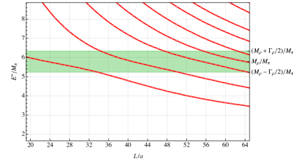
Figure 5: Energy spectrum of a $I=1$, $\ell=1$, $\pi\pi$ system at physical pion mass in a finite cubic volume of side length $aL$ ($a=0.1~{}{\rm fm}$). The spectrum is obtained from Eq. (3.17) using Breit-Wigner parametrization of the phase-shifts with PDG parameters [18]. Periodic boundary conditions are applied and projection to the $T_{1g}$ irrep are performed.

For the zero total momentum case considered here the Eq. (3.17) reduces to

$$\cot(\delta_{1})=\frac{\mathcal{Z}(1;q^{2})}{\pi^{3/2}q}\,,\qquad q=k\frac{L}{2\pi}\,,$$ (3.36)

with $k(E_{\mathrm{cm}})$ defined in Eq. (3.19) with $M\equiv M_{\pi}$ and the Lüscher zeta function

$$\mathcal{Z}(1;q^{2})=\frac{1}{\sqrt{4\pi}}\sum_{\vec{d}\in\mathbb{Z}^{3}}\left(|\vec{d}|^{2}-q^{2}\right)^{-s}\,.$$ (3.37)

Now, one is left to solve Eq. (3.36) numerically for the phase-shift $\delta_{1}$ with $E_{\mathrm{cm}}$ and $M_{\pi}$ as input. Obviously, the procedure can be inverted, predicting the finite-volume spectrum, assuming a specific form of the $\pi\pi$ interaction determining the left-hand-side of Eq. (3.36). For the simple case of Breit-Wigner parametrization discussed in the beginning of this review, the predicted spectrum is depicted in Fig. 5. The distinctive feature of the so-called avoided level crossing is evident there [147].

4 Theoretical methods II: EFTs for resonances

Chiral perturbation theory (CHPT) is the low-energy effective field theory (EFT) of QCD [148, 137, 138]. First and foremost, it is the theory of the Goldstone bosons, the pions in the two-flavor ($u,d$) case and the pions, the kaons and the eta in the three-flavor ($u,d,s$) sector. It has enjoyed considerable successes, see Refs. [149, 150, 151, 152, 153, 154, 155] for reviews. The Goldstone bosons also couple to matter fields, in particular the nucleons (protons and neutrons) in the SU(2) case or the low-lying baryon octet ($N,\Lambda,\Sigma,\Xi$) for three flavors, see, e.g., Refs. [156, 157, 158] for early works and Refs. [159, 159, 160, 161] for reviews. A cornerstone of CHPT is the power counting, which we briefly discuss here. Symbolically, any matrix element admits an expansion in small momenta/energies/masses $Q$ over the hard scale $\Lambda$ of the form

$${\cal M}=\sum_{\nu}\left(\frac{Q}{\Lambda}\right)^{\nu}f_{\nu}(Q/\mu,g_{i})~{},$$ (4.1)

where $\mu$ is a regularization scale (often the scale of dimensional regularization), the $g_{i}$ are low-energy constants (LECs), the $f_{\nu}$ are functions of order one (“naturalness”) and the index $\nu$ is bounded from below, which leads to a systematic and controlled expansion. In case of pure Goldstone boson interactions, $\nu=2$ is the smallest possible value due to the derivative nature of the interactions. This expansion can be mapped onto a well-defined quantum field theory with tree and loop graphs, where the infinite part of the LECs absorb the UV infinities generated by the loop diagrams at a given order.

Since CHPT is an EFT, its range of applicability is limited to momenta and energies below some hard scale. This scale of chiral symmetry breaking $\Lambda_{\chi}$ is often identified as $\Lambda_{\chi}=4\pi F_{\pi}$, with $F_{\pi}\simeq 92\,$MeV the pion decay constant, thus, $\Lambda_{\chi}\simeq 1.2\,$GeV [162]. However, the true limitation to CHPT sets in earlier and is channel-dependent, related to the appearance of certain resonances with appropriate quantum numbers. Prominent examples are the broad $f_{0}(500)$ for pion-pion interactions in the channel with $\ell=I=0$, with $\ell$ and $I$ denoting the total angular momentum and isospin of the two-pion system, respectively, the much narrower $\rho(770)$ for $\ell=I=1$ or the lowest-lying resonance in pion-nucleon scattering, the $\Delta(1232)$. Of course, the appearance of such resonances is not restricted to the light quark sector, but leads to similar limitations in EFTs involving the heavy $c,b$ quarks, as will be discussed later.

Therefore, we need to extend CHPT to cope with resonances. This can be done in two ways. First, one can construct EFTs with explicit resonance fields, see section 4.1. The main obstacle here is the fact that resonances decay and it is not trivial to write down a consistent power counting that accounts for the different momentum/energy scales that necessarily appear. Second, one can use unitarization methods, which amount to a resummation of the chiral expansion similar to the geometric series, that is the expansion of the form $1+x$ is substitute by $1/(1-x)$, which allows for the generation of resonances. This was first done in Refs. [163, 164] and critically re-examined in [165]. The upshot is that such a unitarization procedure induces some model-dependence, as discussed in section 4.5. In a few selected cases, one can combine the chiral expansion with dispersion relations to extract resonance properties, which we will not consider in detail here but rather refer to [166, 44, 167] (and references therein).

4.1 EFTs with explicit resonance fields

Before addressing the ways of explicitly including vector mesons, let us discuss the problems with the power counting that arises for unstable particles. As our prime example, we take the $\rho\to\pi\pi$ decay and follow the arguments given in [168]. Consider the leading one-loop correction to the vector meson mass given by the leftmost diagram in Fig. 6. Denote the integral corresponding to this self-energy contribution by $I$. It can not straightforwardly be calculated because the large vector meson mass $M_{V}$ obscures the power counting as in the case of the nucleon [156]. However, the integral can be split into a “soft” and a “hard” part [169], such that $I=I_{\rm soft}+I_{\rm hard}$, where the soft part is entirely generated by small momenta $Q\ll M_{V}$ and, thus, is consistent with the power counting, whereas the hard part with momenta $Q\simeq M_{V}$ leads to the breaking of the power counting and needs to be treated separately. In a more formal language, this corresponds to the method of dimensional counting [170] or the strategy of regions [171]. In fact, the soft parts of any diagram satisfy the expected power counting. Working out $I_{\rm soft}$, one finds that the result corresponds to a series of tadpole graphs, involving only one Goldstone boson propagator, scaling as ${\cal O}(Q^{3})$. This can of course not be the whole story, because the amplitude of Fig. 6 (leftmost diagram) has an imaginary part due to the production of two Goldstone bosons in the intermediate state, while the tadpole sum does not have such an imaginary part. In order to take only $I_{\rm soft}$ as the regularized amplitude, one would have to write complex coefficients in the effective Lagrangian, which in general, one does not want to do (for an exception, see section 4.2). A direct calculation of the full scalar loop integral shows that the imaginary part indeed does not satisfy the power counting mentioned above, i.e, it does not scale $\sim Q^{3}$ . This is related to the fact that for large external four-momenta squared, $P^{2}$, of the heavy external particle, the Goldstone bosons produced in the decay of this particle are not to be considered as soft. Below the threshold, we have $P^{2}<4M_{\pi}^{2}$, so $P^{2}$ can not be considered as being very large compared to the scale $M_{\pi}^{2}$ in that region, and we would have to take the full integral $I$ as the soft part, and not just $I_{\rm soft}$. This phenomenon of the “missing imaginary part” was also pointed out in the framework of heavy meson effective theory in Ref. [172]. For other approaches to include vector mesons in chiral EFTs, see, e.g., [173, 174, 175, 175, 176, 177, 178, 179, 180]. The case of baryon resonances will be discussed in section 4.4.

Figure 6: Leading one-loop contributions to the $\rho$-meson self-energy. The filled square denotes a counterterm. In the complex mass scheme, the latter is a complex-valued quantity.

4.2 The complex mass scheme

The complex-mass renormalization scheme is a method that was originally introduced for precision $W,\,Z$-physics, see, e.g., [181, 182] and later transported to chiral EFT [183]. Let us first give a brief outline of the complex-mass scheme (CMS), following Ref. [184]. Consider first an instable particle at tree level. The CMS amounts to treating the mass of this particle consistently as a complex quantity, defined as the location of the pole in the complex $k^{2}$-plane of the corresponding propagator with momentum $k$. It can be shown that this scheme is symmetry-preserving and leaves the corresponding Ward identities intact. Extending this to one loop, one splits the real bare masses into complex renormalized masses and complex counterterms. This is important, as only renormalized masses are observable. The corresponding Lagrangian yields Feynman rules with complex masses and counterterms, which allows for standard perturbative calculations. This is essentially a rearrangement of contributions that is not affected by double counting. The imaginary part of the particle mass appears in the propagator and is resummed in the Dyson series. In contrast to this, the imaginary part of the counterterm is not resummed. One can show that in such a case gauge invariance remains valid, and unitarity cancellations are respected order by order in the perturbative expansion. This also requires integrals with complex internal masses, as worked out in Ref. [185]. For further discussions of the method, the reader is referred to Refs. [184, 186] (and references therein). In case of a chiral EFT, the perturbative expansion proceeds as usual in terms of small momenta and quark masses, with a proper treatment of the heavy particle mass in loop diagrams (like the heavy-baryon scheme [157, 158] or the so-called infrared-regularization [187] or the extended-on-mass-scheme discussed below [188]).

Let us now calculate the mass and the width of the $\rho$ within the CMS to leading one-loop order ${\cal O}(Q^{3})$, following Ref. [183]. The pertinent Lagrangian is given by [189, 190, 191, 192]

$${\cal L} = {\cal L}_{\pi}+{\cal L}_{\rho\pi}+{\cal L}_{\omega}+{\cal L}_{\omega\rho\pi}+\ldots~{},$$

$${\cal L}_{\pi}+{\cal L}_{\rho\pi} = \frac{F^{2}}{4}\,\langle\partial_{\mu}U(\partial^{\mu}U)^{\dagger}\rangle+\frac{F^{2}\,M^{2}}{4}\,\langle U^{\dagger}+U\rangle-\frac{1}{2}\,\langle\rho_{\mu\nu}\rho^{\mu\nu}\rangle+\left[M_{\rho}^{2}+\frac{c_{x}\,M^{2}}{4}\,\langle U^{\dagger}+U\rangle\right]\,\langle\hat{\rho}_{\mu}\hat{\rho}^{\mu}\rangle~{},$$

$${\cal L}_{\omega}+{\cal L}_{\omega\rho\pi} = -\frac{1}{4}\omega_{\mu\nu}\omega^{\mu\nu}+\frac{1}{2}M_{\omega}^{2}\,\omega_{\mu}\omega^{\mu}+\frac{1}{2}\,g_{\omega\rho\pi}\,\epsilon_{\mu\nu\alpha\beta}\,\omega^{\nu}\,\langle\rho^{\alpha\beta}u^{\mu}\rangle~{},$$ (4.2)

where

$$U = u^{2}={\rm exp}\left(\frac{\mathrm{i}\vec{\tau}\cdot\vec{\pi}}{F}\right)~{},~{}~{}\Gamma_{\mu}=\frac{1}{2}\,\bigl{[}u^{\dagger}\partial_{\mu}u+u\partial_{\mu}u^{\dagger}\bigr{]}~{},~{}~{}u_{\mu}=\mathrm{i}\left[u^{\dagger}\partial_{\mu}u-u\partial_{\mu}u^{\dagger}\right]~{},$$

$$\rho^{\mu} = \frac{\vec{\tau}\cdot\vec{\rho}\,^{\mu}}{2}~{},~{}~{}\rho^{\mu\nu}=\partial^{\mu}\rho^{\nu}-\partial^{\nu}\rho^{\mu}-\mathrm{i}g\left[\rho^{\mu},\rho^{\nu}\right]~{},~{}~{}\hat{\rho}_{\mu}=\rho_{\mu}-\frac{\mathrm{i}}{g}\Gamma_{\mu}~{},~{}~{}\omega^{\mu\nu}=\partial^{\mu}\omega^{\nu}-\partial^{\nu}\omega^{\mu}~{}.$$ (4.3)

Here, $F$ is the pion decay constant in the chiral limt, $M^{2}$ is the leading term in the quark mass expansion of the pion mass squared, $\langle...\rangle$ denotes a trace in flavor space, $M_{\rho}$ and $M_{\omega}$ refer to the bare $\rho$ and $\omega$ masses, $g$ is the $\rho$-coupling subject to the constraint $M_{\rho}^{2}=2\,g^{2}F^{2}$, the so-called KSFR relation [193, 194], $g_{\omega\rho\pi}$ parameterizes the strength of the $\omega\rho\pi$ vertex and $c_{x}$ is a LEC related to the quark mass expansion of the $\rho$ mass, which also affects the $\rho\to\pi\pi$ vertex. Next, one performs standard renormalization, i.e., the bare parameters (as indicated by a subscript 0) are expressed in terms of the normalized ones and a number of counterterms, leading to (we only display the ones contributing at leading loop order)

$$\rho^{\mu}_{0}=\sqrt{Z_{\rho}}\,\rho^{\mu}~{},~{}~{}M_{\rho,0}=M_{R}+\delta M_{R}~{},~{}~{}c_{x,0}=c_{x}+\delta c_{x}~{}.$$ (4.4)

Now, one applies CMS and chooses

$$M_{R}^{2}=(M_{\chi}-i\,\Gamma_{\chi}/2)^{2}~{},$$ (4.5)

as the pole of the $\rho$-meson propagator in the chiral limit, where the pole mass and the width of the $\rho$ meson in the chiral limit are denoted by $M_{\chi}$ and $\Gamma_{\chi}$, respectively. These are input parameters. In this scheme, one includes $M_{R}$ in the propagator and the counterterms, which are complex-valued quantities now, are treated perturbatively. As noted before, the mass of the $\rho$ is not a small quantity, thus, one has to specify a power counting that accounts for that. Let $Q$ collectively denote a small quantity. The pion propagator counts as ${\cal O}(Q^{-2})$ if it does not carry large external momenta and as ${\cal O}(Q^{0})$ if it does. The vector-meson propagator counts as ${\cal O}(Q^{0})$ if it does not carry large external momenta and as ${\cal O}(Q^{-1})$ if it does. The pion mass counts as ${\cal O}(Q^{1})$, the vector-meson mass as ${\cal O}(Q^{0})$, and the width as ${\cal O}(Q^{1})$. Vertices generated by the effective Lagrangian of Goldstone bosons ${\cal L}_{\pi}^{(n)}$ count as ${\cal O}(Q^{n})$. Derivatives acting on heavy vector mesons, which cannot be eliminated by field redefinitions, count as ${\cal O}(Q^{0})$. The contributions of vector meson loops can be absorbed systematically in the renormalization of the parameters of the effective Lagrangian. Therefore, such loop diagrams need not be included for energies much lower than twice the vector-meson mass. Note also that the smallest order resulting from the various assignments is defined as the chiral order of the given diagram.

Now we are in the position to evaluate the two-point function (2PF). The mass and width of the $\rho$ meson are extracted from the complex pole of the 2PF. The 2PF, that is the sum of all one-particle irreducible diagrams, is parameterized as

$$\Pi^{ab}_{\mu\nu}(p)=\delta^{ab}\,\left[g_{\mu\nu}\Pi_{1}(p^{2})+p_{\mu}p_{\nu}\,\Pi_{2}(p^{2})\right]\,.$$ (4.6)

The dressed propagator, expressed in terms of the self-energy, has the form

$$S^{ab}_{\mu\nu}(p)=-\delta^{ab}\,\frac{g_{\mu\nu}-p_{\mu}p_{\nu}\left(1+\Pi_{2}(p^{2})\right)\left(M_{R}^{2}+\Pi_{1}(p^{2})+p^{2}\Pi_{2}(p^{2})\right)^{-1}}{p^{2}-M_{R}^{2}-\Pi_{1}(p^{2})+\mathrm{i}\,\eta}\,,$$ (4.7)

with $\eta\to 0^{+}$ and the pole of the propagator is found as the (complex) solution to the equation:

$$z-M_{R}^{2}-\Pi_{1}(z)=0\,.$$ (4.8)

In the vicinity of the pole $z$, the dressed propagator takes the form

$$S^{ab}_{\mu\nu}(p)=-\delta^{ab}\left[\frac{Z^{r}_{\rho}\left(g_{\mu\nu}-{p_{\mu}p_{\nu}}/{z}\right)}{p^{2}-z+\mathrm{i}\,\eta}+R\right]\,,$$ (4.9)

where $Z^{r}_{\rho}={1}/({1-\Pi_{1}^{\prime}(z)})$ and $R$ denotes the non-pole part (the remainder). The counterterms $\delta M_{R}$ and $\delta Z_{\rho}$ are fixed by requiring that in the chiral limit $M_{R}^{2}$ is the pole of the dressed propagator and that the residue $Z_{\rho}^{r}$ is equal to one. The solution to Eq. (4.8) admits a perturbative expansion of the form

$$z=z^{(0)}+z^{(1)}+z^{(2)}+\ldots\,,$$ (4.10)

where the superscripts $(i)$ denote the $i^{\rm th}$ loop order. All of these terms further admit a chiral expansion. For example, the tree level result to third order in the chiral expansion reads $z^{(0)}=M_{R}^{2}+c_{x}M^{2}$, which is consistent with the general result for the quark mass expansion of the vector meson mass [168]. More interesting is the result at leading one-loop order. The corresponding contributions to the self-energy are depicted in Fig. 6. The contributions of the pion loop and the $\pi\omega$ loop to $\Pi_{1}$ are given by

$$D_{\pi\pi} = -\frac{g^{2}\mu^{4-n}}{d-1}\,\left[2\,I_{M}-\left(P^{2}-4M^{2}\right)\,I_{MM}\right]\,,$$

$$D_{\pi\omega} = \frac{(d-2)\,g_{\omega\rho\pi}^{2}\,\mu^{4-d}}{4\,(d-1)}\,\left[M^{4}\,I_{MM_{\omega}}-\left(2\,I_{MM_{\omega}}M_{\omega}^{2}+I_{M}-I_{M_{\omega}}+2\,I_{MM_{\omega}}P^{2}\right)M^{2}\right.$$ (4.11)

$$\left.+I_{MM_{\omega}}P^{2}+M_{\omega}^{2}\left(I_{MM_{\omega}}M_{\omega}^{2}+I_{M}-I_{M_{\omega}}\right)-\left(2I_{MM_{\omega}}M_{\omega}^{2}+I_{M}+I_{M_{\omega}}\right)P^{2}\right]\,,$$

in terms of the loop integrals

$$I_{m_{1}m_{2}} = \frac{\mathrm{i}}{(2\pi)^{d}}\,\int\frac{d^{d}k}{\left[k^{2}-m_{1}^{2}+\mathrm{i}\,0^{+}\right]\left[(P+k)^{2}-m_{2}^{2}+\mathrm{i}\,0^{+}\right]}\,,$$

$$I_{m} = \frac{\mathrm{i}}{(2\pi)^{d}}\,\int\frac{d^{d}k}{k^{2}-m^{2}+\mathrm{i}\,0^{+}}\,,$$ (4.12)

with $d$ the number of space-time dimensions, $\mu$ the scale of dimensional regularization and $P$ the four-momentum of the vector meson. Note, however, that the $\pi\pi$-loop only starts to contribute at ${\cal O}(Q^{4})$ to $\Pi_{1}$, as the large component is $\propto P^{\mu}$. Note further that this diagram contains a power-counting violating imaginary part, which is cancelled by the imaginary part of the complex counterterm, see Fig. 6. This is the major advantage of the CMS scheme. In the calculation of the $\pi\omega$ loop, one uses $M_{\omega}=M_{\rho}$, which is good approximation ($\rho$-$\omega$ mixing in chiral EFT is discussed in Refs. [195, 196, 197, 198], see also the review [199]). Next, the counterterm contributions are adjusted such that the pole in the chiral limit stays at $M_{R}$, leading to

$$\delta M_{R} = -\frac{1}{3}\,g^{2}M_{R}\,\lambda+\frac{g^{2}}{288\,\pi^{2}}M_{R}\left(-3\ln(M_{R}^{2}/\mu^{2})+3\mathrm{i}\pi+5\right)+\frac{1}{3}g_{\omega\rho\pi}^{2}M_{R}^{3}\lambda+\frac{g_{\omega\rho\pi}^{2}}{288\pi^{2}}M_{R}^{3}\left(3\ln(M_{R}^{2}/\mu^{2})+1\right)\,,$$

$$\delta c_{x} = 4g^{2}\lambda-\frac{g^{2}}{8\pi^{2}}\left(1-\ln(M_{R}^{2}/\mu^{2})+\mathrm{i}\pi\right)+g_{\omega\rho\pi}^{2}M_{R}^{2}\lambda-\frac{g_{\omega\rho\pi}^{2}}{32\pi^{2}}M_{R}^{2}\left(1-\ln({M_{R}^{2}}/{\mu^{2}})\right)\,,$$

$$\lambda = \frac{1}{16\,\pi^{2}}\left\{\frac{1}{d-4}-\frac{1}{2}\,\left[\ln(4\pi)+\Gamma^{\prime}(1)+1\right]\right\}\,,$$ (4.13)

with $\Gamma^{\prime}(1)=0.5772$ the Euler-Mascheroni constant. Note that these terms all involve powers of the large mass $M_{R}$ and are, thus, power-counting violating. However, they can all be absorbed in the complex-valued counterterms. Using now the renormalized version of the KSFR relation, one can eliminate the coupling $g$ and obtains for the pole mass and the width of the $\rho$ meson by expanding the contributions to ${\cal O}(Q^{4})$

$$M_{\rho}^{2} = M_{\chi}^{2}+c_{x}M^{2}_{\pi}-\frac{g_{\omega\rho\pi}^{2}M^{3}_{\pi}M_{\chi}}{24\pi}+\frac{M^{4}_{\pi}}{32\pi^{2}F^{2}_{\pi}}\left(3-2\,\ln(M^{2}_{\pi}/M_{\chi}^{2})\right)-\frac{g_{\omega\rho\pi}^{2}}{32\pi^{2}}M^{4}_{\pi}\left(\ln(M^{2}_{\pi}/M_{\chi}^{2})-1\right)\,,$$ (4.14)

$$\Gamma = \Gamma_{\chi}+\frac{\Gamma_{\chi}^{3}}{8M_{\chi}^{2}}-\frac{c_{x}\Gamma_{\chi}M^{2}_{\pi}}{2M_{\chi}^{2}}-\frac{g_{\omega\rho\pi}^{2}M^{3}_{\pi}\Gamma_{\chi}}{48\pi\,M_{\chi}}+\frac{M^{4}_{\pi}}{16\,\pi\,F^{2}_{\pi}M_{\chi}}\,,$$ (4.15)

where we have identified the leading terms in the quark mass expansion of the pion mass and the pion decay constant with their physical values. A few more remarks are in order. Since the power-counting breaking terms are all absorbed, we end up with a well behaved chiral expansion featuring terms $\sim\!M^{2}_{\pi},M^{3}_{\pi}$ and $M^{4}_{\pi}$. Note further that there will be finite contributions from the neglected diagrams of ${\cal O}(Q^{4})$ but no new non-analytic terms. This agrees with the general structure of the chiral expansion worked out in [168]. The non-analytic terms displayed here agree with the calculation of Ref. [200]. To get an idea about the size of the corrections, one plugs in $F_{\pi}=0.092\,{\rm GeV},M_{\pi}=0.139\,{\rm GeV}\,,g_{\omega\rho\pi}=16\,{\rm GeV^{-1}},M_{\chi}\approx M_{\rho}=0.78\,{\rm GeV}$ and obtains $M_{\rho}^{2}=M_{\chi}^{2}+0.019c_{x}-0.0044$ (in GeV²) and $\Gamma=\Gamma_{\chi}+0.21\Gamma_{\chi}^{3}-0.016c_{x}\Gamma_{\chi}-0.0058\Gamma_{\chi}+0.0011$ (in GeV). One notices that the corrections to the chiral limit mass are rather small, as also found in Ref. [168]. In section 5, we will use Eqs. (4.14,4.15) to analyze lattice QCD data from the ETMC collaboration. For further work on vector meson properties using the CMS, see Refs. [201, 202].

4.3 The complex mass scheme at two loops

It is important to consider the CMS beyond the one-loop level, as discussed below on the examples of the decay $\omega\to 3\pi$, $\Delta\to N\pi$ or the Roper decays $N^{*}(1440)\to N\pi,N\pi\pi$. We will first show on the example of the first decay that the CMS can indeed by extended to two-loop order and then use this knowledge to derive so far unknown constraints on the mentioned baryon decay modes.

Consider first the $\omega$ meson. As its main decay is $\omega\to 3\pi$, the self-energy has its first non-trivial contribution at two-loop order, see the left diagram in Fig. 7, where the $\omega$ is represented by the solid line and the dashed lines denote pions. The leading interaction Lagrangian reads [190]:

$${\cal L}_{V\Phi\Phi\Phi}^{(1)}=\frac{\mathrm{i}\,h}{4F_{\pi}^{3}}\,\epsilon^{\mu\nu\alpha\beta}\,\langle V_{\mu}\partial_{\nu}\Phi\partial_{\alpha}\Phi\partial_{\beta}\Phi\rangle~{},$$ (4.16)

with $V_{\mu}$ the vector field corresponding to the $\omega$ meson, the pions are given by $\Phi=\pi^{a}\tau^{a}$, as we are considering two flavors here, and $h$ is a coupling constant. The self-energy corresponding to this two-loop diagram takes the form:

$$\Sigma^{\mu\nu} = \frac{72\pi^{2}h^{2}}{F_{\pi}^{6}}\,\left(p^{\mu}p^{\nu}-p^{2}g^{\mu\nu}\right)I_{d+2}~{},$$

$$I_{d+2} = \frac{1}{(2\pi)^{2(d+2)}}\int\frac{d^{d+2}k_{1}d^{d+2}k_{2}}{\left[k_{1}^{2}-M^{2}+\mathrm{i}\eta\right]\left[k_{2}^{2}-M^{2}+i\eta\right]\left[(p+k_{1}+k_{2})^{2}-M^{2}+\mathrm{i}\eta\right]}~{},$$ (4.17)

with $\eta\to 0^{+}$ and $d$ is the number of space-time dimension. We see that the study of the $\omega$ self-energy reduces to a scalar integral in six dimension. To further analyze this self-energy, while avoiding any complications due to the spin and chiral symmetry, the authors of Ref. [203] investigated a field theoretical model Lagrangian of interacting scalar fields in six space-time dimensions

$$\mathcal{L}=\frac{1}{2}(\partial_{\mu}\pi\partial^{\mu}\pi-M^{2}\pi^{2})+\frac{1}{2}(\partial_{\mu}\Psi\partial^{\mu}\Psi-m^{2}\Psi^{2})-\frac{g}{3!}\,\pi^{3}\Psi+\mathcal{L}_{1}~{},$$ (4.18)

where the masses of the light and heavy scalar fields $\pi$ and $\Psi$, respectively, satisfy the condition $M\ll m$, since $\Psi$ represents an unstable particle. This Lagrangian $\mathcal{L}_{1}$ contains all possible terms which are consistent with Lorentz symmetry and with the invariance under the simultaneous transformations $\pi\to-\pi$ and $\Psi\to-\Psi$. The power counting is build on small quantities $Q$ like the mass $M$, small external four-momenta of the $\pi$ or small external three-momenta of the $\Psi$. The two-loop diagram shown in Fig.  7 should, thus, scale as $Q^{(2d-4)}$, which at first sight is messed up due to the complications generated by the large scale $m$. However, using the “dimensional counting analysis” of Ref. [170] or, equivalently, the “strategy of regions” [171], after some lengthy algebra, one can identify and subtract the power counting breaking terms generated from the heavy scale $m$. These are canceled exactly by the complex counterterms that appear in the one-loop and tree-level diagrams at this order, see Fig. 7. More precisely, the one-loop counterterms originate from the one-loop diagrams contributing to elastic $\pi\Psi$ scattering, whereas the two-loop counterterm arises from a subset of the terms in the Lagrangian ${\mathcal{L}}_{1}$. Thus, the CMS scheme is also applicable at two-loop order, and it leads to a consistent power counting, if and only if the subtraction of one-loop sub-diagrams in the renormalization of the two-loop diagrams is properly done, for details see [203]. Calculations using the chiral effective Lagrangians are more involved due to the complicated structure of the interactions, but the general features of the renormalization program do not change.

Figure 7: Self-energy at two loops for a heavy particle (solid lines) coupling to light particles (dashed lines). The filled square and the filled circle denote a one-loop and a two-loop counterterm, respectively.

4.4 The width of the lightest baryon resonances from EFT

We now consider the width of the two lowest baryon resonances, the $\Delta(1232)$ and the Roper $N(1440)$ at two-loop order in the CMS. Ultimately, these widths should be calculated on the lattice, see Sect. 3, but the detailed two-loop studies reveal in the case of the $\Delta(1232)$ some intriguing correlations bewteen LECs, that will also be useful in a presicion extraction from lattice QCD data, and in case of the Roper give insights into the important decay into a nucleon and two pions. Other resonances like, e.g., the $\Lambda(1405)$ have also been considered as explicit fields in chiral Lagrangians, see, e.g., Refs. [204, 205], but in such cases that involve coupled-channels, unitarization methods are superior. These are discussed in section 4.5.

Consider first the $\Delta(1232)$-resonance. Here, the new small scale $\Delta\equiv m_{\Delta}-m_{N}\simeq 300\,$MeV arises, that must be dealt with consistently and also, it is known that the $\Delta$ couples strongly to the $N\pi$ system, making it an important ingredient in nuclear physics [206]. Extensions of CHPT including the Delta (or the decuplet baryons in the three-flavor case) have been pioneered in Refs. [207, 208, 209, 210, 211], where in particular in the last two references, the so-called small scale expansion (SSE) has been introduced. In the SSE, the set of small parameters is extended to include the Delta-nucleon mass splitting,

$$Q\in\left\{\frac{p}{\Lambda},\frac{M_{\pi}}{\Lambda},\frac{\Delta}{\Lambda}\right\}~{},$$ (4.19)

and one often uses $\epsilon$ instead of $Q$ to distinguish from the standard case with $\Delta=0$. For other approaches to include these spin-3/2 fields, see, e.g., Refs. [212, 213, 214, 215, 216, 217, 218, 219, 220, 221, 222, 223]. It is important to note that the splitting $m_{\Delta}-m_{N}$ does not vanish in the chiral limit, which has important consequences for the corresponding EFT [224, 225, 226]. The decoupling of the Delta in the chiral limit enforces that contributions involving the spin-3/2 field must vanish as $\Delta\to\infty$. Explicit examples are worked out in [225]. However, in the limit of colors, $N_{c}$, going to infinity [227, 228] the situation is opposite, namely the Delta becomes degenerate with the nucleon and, thus, can not be integrated out. The consequences of this scenario have been first worked out in Refs. [229, 230, 231], for an early review see [232] and further work, e.g., in Refs. [233, 234, 235, 236, 237, 238, 237, 239, 240].

4.4.1 The width of the $\Delta(1232)$

Consider first the width of the $\Delta$ at two-loop order [241]. The pertinent effective Lagrangian contains, besides many other terms, the leading $\pi\Delta$ and $\pi N\Delta$ couplings, parametrized in terms of the LECs $g_{1}$ and $h$, respectively,

$${\cal L}^{(1)}_{\pi\Delta} = -\bar{\Psi}_{\mu}^{i}\xi^{\frac{3}{2}}_{ij}\Bigl{\{}\left(\mathrm{i}\not{D}^{jk}-m_{\Delta}\delta^{jk}\right)g^{\mu\nu}-\mathrm{i}\left(\gamma^{\mu}D^{\nu,jk}+\gamma^{\nu}D^{\mu,jk}\right)+\mathrm{i}\gamma^{\mu}\not{D}^{jk}\gamma^{\nu}+m_{\Delta}\delta^{jk}\gamma^{\mu}\gamma^{\nu}$$

$$+{g_{1}}\frac{1}{2}\not{u}^{jk}\gamma_{5}g^{\mu\nu}+g_{2}\frac{1}{2}(\gamma^{\mu}u^{\nu,jk}+u^{\nu,jk}\gamma^{\mu})\gamma_{5}+g_{3}\frac{1}{2}\gamma^{\mu}\not{u}^{jk}\gamma_{5}\gamma^{\nu}\Bigr{\}}\xi^{\frac{3}{2}}_{kl}{\Psi}_{\nu}^{l}\,,$$

$${\cal L}^{(1)}_{\pi N\Delta} = h\,\bar{\Psi}_{\mu}^{i}\xi_{ij}^{\frac{3}{2}}\Theta^{\mu\alpha}(z_{1})\ \omega_{\alpha}^{j}\Psi_{N}+{\rm h.c.}\,,$$ (4.20)

$${\cal L}^{(2)}_{\pi N\Delta} = \bar{\Psi}_{\mu}^{i}\xi_{ij}^{\frac{3}{2}}\Theta^{\mu\alpha}(z_{2})\,\left[\mathrm{i}\,b_{3}\omega_{\alpha\beta}^{j}\gamma^{\beta}+\mathrm{i}\,\frac{b_{8}}{m}\omega_{\alpha\beta}^{j}i\,D^{\beta}\right]\Psi_{N}+{\rm h.c.}\,,$$

$${\cal L}^{(3)}_{\pi N\Delta} = \bar{\Psi}_{\mu}^{i}\xi_{ij}^{\frac{3}{2}}\Theta^{\mu\nu}(z_{3})\biggl{[}\frac{f_{1}}{m}[D_{\nu},\omega_{\alpha\beta}^{j}]\gamma^{\alpha}\mathrm{i}\,D^{\beta}-\frac{f_{2}}{2m^{2}}[D_{\nu},\omega_{\alpha\beta}^{j}]\{D^{\alpha},D^{\beta}\}+f_{4}\omega_{\nu}^{j}\langle\chi_{+}\rangle+f_{5}[D_{\nu},\mathrm{i}\chi_{-}^{j}]\biggr{]}\Psi_{N}+{\rm h.c.}\,,$$

where $\Psi_{N}$ and $\Psi_{\nu}$ are the isospin doublet field of the nucleon and the vector-spinor isovector-isospinor Rarita-Schwinger field of the $\Delta$-resonance with bare masses $m$ and $m_{\Delta 0}$, respectively. $\xi^{\frac{3}{2}}$ is the isospin-$3/2$ projector, $\omega_{\alpha}^{i}=\frac{1}{2}\,\langle\tau^{i}u_{\alpha}\rangle$ and $\Theta^{\mu\alpha}(z)=g^{\mu\alpha}+z\gamma^{\mu}\gamma^{\alpha}$. Using field redefinitions the off-shell parameters $z$ can be absorbed in LECs of other terms of the effective Lagrangian and, therefore, they can be chosen arbitrarily [242, 243]. We fix the off-shell structure of the interactions with the Delta by adopting $g_{2}=g_{3}=0$ and $z_{1}=z_{2}=z_{3}=0$. Thus, $g_{1}$ parameterizes the leading $\pi\Delta$ vertex. For vanishing external sources, the covariant derivatives are given by

$$D_{\mu}\Psi_{N} = \left(\partial_{\mu}+\Gamma_{\mu}\right)\Psi_{N}\,,~{}~{}~{}\Gamma_{\mu}=\frac{1}{2}\,\left[u^{\dagger}\partial_{\mu}u+u\partial_{\mu}u^{\dagger}\right]=\tau_{k}\Gamma_{\mu,k}\,,$$

$$\left(D_{\mu}\Psi\right)_{\nu,i} = \partial_{\mu}\Psi_{\nu,i}-2\,\mathrm{i}\,\epsilon_{ijk}\Gamma_{\mu,k}\Psi_{\nu,j}+\Gamma_{\mu}\Psi_{\nu,i}\,.$$ (4.21)

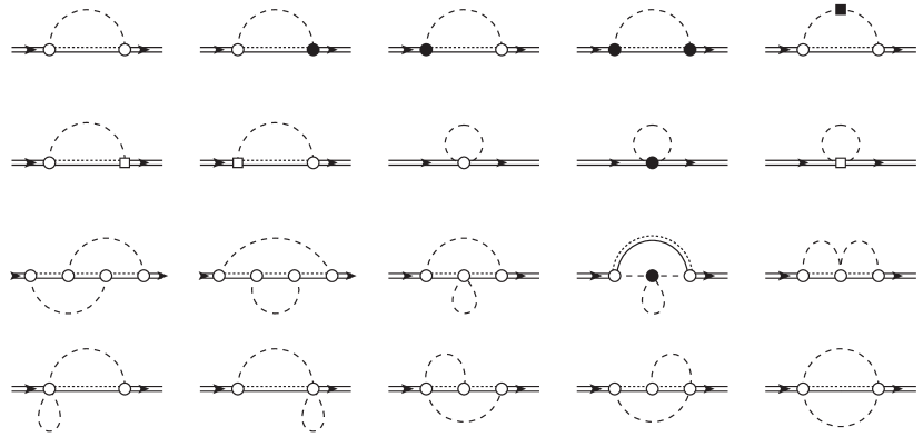
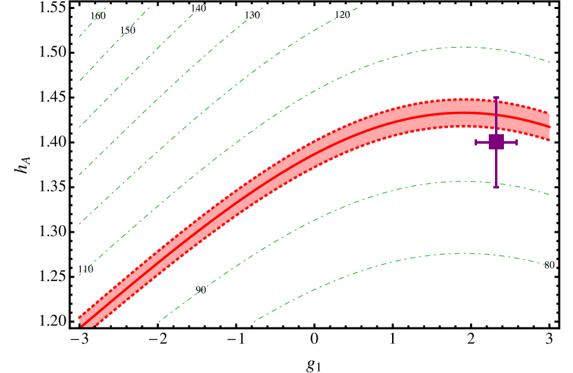
Figure 8: Left panel: One and two-loop self-energy diagrams contributing to the width of the Delta resonance up-to-and-including fifth order according to the standard power counting. The dashed and double solid lines represent the pions and the Delta resonances, respectively. The double (solid-dotted) lines in the loops correspond to either nucleons or Deltas. Open and filled circles refer to LO and NLO vertices from the meson-baryon Lagrangian, where as the filled box represents an NLO mesonic term. Right panel: Correlation between the leading $\pi\Delta$ and $\pi N\Delta$ couplings. The central line corresponds to $\Gamma_{\Delta}=100$ MeV while the band is obtained by varying $\Gamma_{\Delta}$ in the range of 98 to 102 MeV. The dot-dashed lines show the correlation for other values of the width of the Delta. The box with the error bars are the results from the analysis of Ref. [244]. Figure adopted from [241].

The power counting relies on the fact that $m_{\Delta}-m_{N}$ is a small quantity. More precisely, the small parameters are the external momenta, the pion mass and the nucleon-Delta mass splitting, collectively denoted as $\varepsilon$. However, there are many LECs in Eq. (4.4.1), so how can one one possibly make any prediction? Let us evaluate the $\Delta$ self-energy at the complex pole,

$$z-m_{\Delta}^{0}-\Sigma(z)=0\quad{\rm with}\quad z=m_{\Delta}-\mathrm{i}\,\displaystyle\frac{\Gamma_{\Delta}}{2}~{}.$$ (4.22)

The corresponding diagrams for the one- and two-loop self-energy contributing to the width of the Delta resonance up to order $\varepsilon^{5}$ are displayed in Fig. 8 (left panel), where the counterterm diagrams are not shown. The one-loop diagrams are easily worked out. For the calculation of the two-loop graphs one uses the Cutkosky rules for unstable particles, that relate the width to the pion-nucleon scattering amplitude, $\Gamma_{\Delta}\sim|A(\Delta\to N\pi)|^{2}$ [245]. One finds a remarkable reduction of parameters that is reflected in the relation

$$h_{A} = h-\left(b_{3}\Delta_{23}+b_{8}\,\Delta_{123}\right)-\left(f_{1}\Delta_{23}+f_{2}\,\Delta_{123}\right)\Delta_{123}+2(2f_{4}-f_{5})M_{\pi}^{2}~{},$$

$$\Delta_{23} = -\Delta=m_{N}-m_{\Delta}~{},~{}~{}~{}~{}\Delta_{123}=\frac{M_{\pi}^{2}+m_{N}^{2}-m_{\Delta}^{2}}{2m_{N}}~{},$$ (4.23)

which means that all of the LECs appearing in the $\pi N\Delta$ interaction at second and third order, the $b_{i}\,(i=3,8)$ and $f_{i}\,(i=1,2,4,5)$, respectively, merely lead to a renormalization of the LO $\pi N\Delta$ coupling $h$,

$$h_{A}=h-\left(b_{3}\Delta_{23}+b_{8}\,\Delta_{123}\right)-\left(f_{1}\Delta_{23}+f_{2}\,\Delta_{123}\right)\Delta_{123}+2(2f_{4}-f_{5})M_{\pi}^{2}~{},$$ (4.24)

and, consequently, one finds a very simple formula for the decay width $\Delta\to N\pi$,

$$\Gamma(\Delta\to N\pi)=\left(53.9\,{h}_{A}^{2}+0.9g_{1}^{2}{h}_{A}^{2}-3.3g_{1}{h}_{A}^{2}-1.0\,{h}_{A}^{4}\right)~{}{\rm MeV}~{}.$$ (4.25)

This leads to a novel correlation that is independent of the number of colors, as $N_{c}$ was not used as a parameter in the calculation. This correlation between $h_{A}$ and $g_{1}$ is depicted in the right panel of Fig. 8. It is obviously fulfilled by the analysis of Ref. [246], that showed that the inclusion of the $\Delta$ alleviates the tension between the threshold and subthreshold regions in the description of $\pi N$ scattering found in baryon CHPT, see also [247].

4.4.2 The width of the Roper resonance

Next, consider the calculation of the width of the Roper-resonance, the $N^{*}(1440)$, at two-loop order [248], improving the one-loop results from Ref. [183]. A remarkable feature of the Roper is the fact that its decay width into a nucleon and a pion is similar to the width into a nucleon and two pions, $\Gamma(R\to N\pi)\simeq\Gamma(R\to N\pi\pi)$. Any model that is supposed to describe the Roper must account for this fact. In CHPT, consider the effective chiral Lagrangian of pions, nucleons and Deltas coupled to the Roper [249, 250, 251],

$${\cal L}_{\rm eff} = {\cal L}_{\pi\pi}+{\cal L}_{\pi N}+{\cal L}_{\pi\Delta}+{\cal L}_{\pi R}+{\cal L}_{\pi N\Delta}+{\cal L}_{\pi NR}+{\cal L}_{\pi\Delta R}~{},$$ (4.26)

with

$${\cal L}_{\pi R}^{(1)} = \bar{\Psi}_{R}\left\{i\not{D}-m_{R}+\frac{1}{2}{g_{R}}\not{u}\gamma^{5}\right\}\Psi_{R}~{},$$

$${\cal L}_{\pi R}^{(2)} = \bar{\Psi}_{R}\left\{c_{1}^{R}\langle\chi_{+}\rangle\right\}\Psi_{R}+\ldots~{},$$

$${\cal L}_{\pi NR}^{(1)} = \bar{\Psi}_{R}\left\{\frac{1}{2}{g_{\pi NR}}\gamma^{\mu}\gamma_{5}u_{\mu}\right\}\Psi_{N}+{\rm h.c.}~{},$$

$${\cal L}^{(1)}_{\pi\Delta R} = {h_{R}}\,\bar{\Psi}_{\mu}^{i}\xi_{ij}^{\frac{3}{2}}\Theta^{\mu\alpha}(\tilde{z})\ \omega_{\alpha}^{j}\Psi_{R}+{\rm h.c.}~{},$$ (4.27)

where $g_{R}$, $g_{\pi NR}$ and $h_{R}$, respectively, are the leading Roper-pion, Roper-nucleon-pion and Delta-Roper-pion couplings. Here, ${\Psi}_{R}$ denotes the Roper isospin doublet field and all other notations are as in the preceding subsection and in Ref. [248].

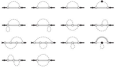
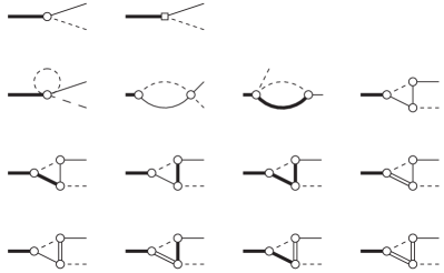
Figure 9: Left panel: One and two-loop self-energy diagrams of the Roper resonance up-to-and-including fifth order according to the standard power counting. The dashed and thick solid lines represent the pions and the Roper resonances, respectively. The thin solid lines in the loops stand for either nucleons, Roper or Delta resonances. For further notations, see Fig. 8. Right panel: Feynman diagrams contribution to the decay $R\to N\pi$ up to leading one-loop order. Dashed, solid, double and thick solid lines correspond to pions, nucleons, Deltas and Roper resonances, respectively.

In this case, the power counting is more complicated, but can be set up around the complex pole of the Roper resonance as (for more details, see [248]), assigning the following counting rules:

$$m_{R}-m_{N}\sim\varepsilon~{},~{}~{}m_{R}-m_{\Delta}\sim\varepsilon^{2}~{},~{}~{}m_{\Delta}-m_{N}\sim\varepsilon^{2}~{},~{}~{}M_{\pi}\sim\varepsilon^{2}~{},$$ (4.28)

where $\varepsilon$ denotes a small parameter. Again, let us calculate the self-energy to two loops at the complex pole $z_{R}=m_{R}-\mathrm{i}\Gamma_{R}/2$. The pertinent diagrams are shown in the left panel of Fig. 9. By applying the cutting rules to these self-energy diagrams, one obtains the graphs contributing to the decay amplitudes of the Roper resonance into the $\pi N$ and $\pi\pi N$ systems, leading to the total width

$$\Gamma_{R}=\Gamma_{R\to N\pi}+\Gamma_{R\to N\pi\pi}~{}.$$ (4.29)

A somewhat lengthy calculation of the diagrams in the right panel of Fig. 9 leads to:

$$\Gamma(R\to N\pi)=550(58)\,g_{\pi NR}^{2}\ {\rm MeV}~{},$$ (4.30)

while the two-pion decay is given at this order by tree diagrams with intermediate nucleons and Deltas,

$$\Gamma(R\to N\pi\pi) = \Bigl{(}1.5(0.6)\,g_{A}^{2}\,g_{\pi NR}^{2}-2.8(1.0)\,g_{A}\,g_{\pi NR}^{2}\,g_{R}+1.5(0.6)\,g_{\pi NR}^{2}\,g_{R}^{2}$$ (4.31)

$$~{}+3.0(1.0)\,g_{A}\,g_{\pi NR}\,h_{A}h_{R}-3.8(1.4)\,g_{\pi NR}\,g_{R}\,h_{A}h_{R}+9.9(5.5)\,h_{A}^{2}h_{R}^{2}\Bigr{)}~{}{\rm MeV}\,.$$

The total width, thus, depends on five LECs. The uncertainties in the round brackets are generated by the uncertainties in the LECs. We use $g_{A}=1.27$ and $h_{A}=1.42\pm 0.02$. The latter value is the real part of this coupling taken from Ref. [244]. As for the other unknown parameters, the authors of [248] fixed $g_{\pi NR}$ so as to reproduce the width $\Gamma_{R\to\pi N}=(123.5\pm 19.0)$ MeV from the PDG. This yields $g_{\pi NR}=\pm(0.47\pm 0.04)$. In what follows, let us take the positive sign for our central value and use the negative one as part of the error budget. Further, assume $g_{R}=g_{A}$ and $h_{R}=h_{A}$, the so-called maximal mixing assumption [252]. Then, one can make a prediction for the two-pion decay width of the Roper,

$$\Gamma(R\to N\pi\pi)=(41\pm 22_{\rm LECs}\pm 17_{\rm h.o.})~{}{\rm MeV}~{},$$ (4.32)

which is consistent with the PDG value of ($67\pm 10$) MeV. The error due to the neglect of the higher orders (h.o.) is simply estimated by multiplying the $\varepsilon^{5}$ result (central value) with $\varepsilon=(m_{R}-m_{N})/m_{N}\simeq 0.43$. Clearly, to make further progress, we need an improved determination of the LECs $g_{R}$ and $h_{R}$. This could be addressed within LQCD. Note also that this scheme has been used to consider the electromagnetic transition form factors of the Roper [253].

4.5 Unitarization methods

4.5.1 General discussion

In the last section we have seen that perturbative calculations based on the effective field theories indeed can allow one to access properties of certain resonances. Such a methodology is advantageous insofar as it allows to separate and identify in a systematic way the dominant (long-range) effects from short-range physics. However, it can only be applied to well separated, low-lying resonances as otherwise no consistent power counting scheme can be set up. In the present section we discuss another class of genuinely non-perturbative approaches. These allow one to deal with the effects of coupled channels and higher-lying resonances, but of course one has to pay a certain prize, as discussed below.

Lattice QCD is a tool to access QCD Green’s functions and transition amplitudes in a non-perturbative and systematical way. However, since the energies and momenta are inherently real, the extraction of resonance parameters requires again an additional step, the analytical continuation to complex energies. This again requires knowledge of analytical expression of the transition amplitudes as functions of, e.g., Mandelstam variables, see section 2. As discussed there, $S$-matrix unitarity plays a crucial role constraining the form of such amplitudes, leading in, e.g., the two-body case to the famous K-matrix parametrization eq. 2.9. In that, the typical workflow includes defining a general parametrization of the real-valued K-matrix (using, e.g., Padé, Chew-Mandelstam forms), fixing the parameters of such expressions from fits to either experimental or lattice results and finally the extraction of poles for complex-valued energies. In this sense also modern statistical and machine learning techniques can indeed be utilized to reduce the parameter space as shown for example in Ref. [254]. More details on such data driven techniques can be found in recent reviews [81, 15]. Dealing with QCD at low energies, chiral symmetry can further lead to additional constraints on transition amplitudes. In regard of lattice QCD results, this is enormously useful allowing one to trace out the quark mass dependence of amplitudes and ultimately resonance parameters. This methodology runs under the name of chiral extrapolations, see section 3.6 and fig. 4 for an explicit example. Such constraints can even be wrapped up in model-independent conditions of functional form of, e.g., resonant $\pi\pi$ amplitudes [255]. Reversing this logic, one can also use low-energy effective theories (such as CHPT) to identify dominant interaction extending the region of applicability by the so-called unitarization procedure.

For pedagogical reasons we begin with the scalar $\phi^{4}$-theory which allows for a simpler treatment. Later we will show how this applies to chiral Lagrangians, leading to the so-called Chiral Unitary approaches(UCHPT) or unitarization schemes. The Lagrangian of the $\phi^{4}$-theory reads

$$\mathcal{L}=\frac{1}{2}\left(\partial^{\mu}\phi\partial_{\mu}\phi-M^{2}\phi^{2}\right)-\frac{\lambda}{4!}\phi^{4}\,,$$ (4.33)

with $M$ the particle mass and $\lambda$ a coupling constant. This simple form of the interaction leads to the fact that the scattering amplitude for the process $\phi(p_{1})\phi(p_{2})\to\phi(p_{1}^{\prime})\phi(p_{2}^{\prime})$ separates into an infinite series of Feynman diagrams ordered in powers of $\lambda$. Specifically, the first two terms of this series read

$$\mathcal{M}_{1}(p_{1}^{\prime},p_{1};p) =-\lambda\,,$$

$$\mathcal{M}_{2}(p_{1}^{\prime},p_{1};p) =-\lambda^{2}\left(\tilde{G}(p_{1}+p_{2})+\tilde{G}(p_{1}-p_{1}^{\prime})+\tilde{G}(p_{1}-p_{2}^{\prime})\right)\,,$$ (4.34)

abbreviating $\mathcal{M}(p_{1}^{\prime},p_{1};p)$ as $\mathcal{M}(p_{1},p_{2}\to p_{1}^{\prime},p_{2}^{\prime})$ with $p=p_{1}^{(\prime)}+p_{2}^{(\prime)}$. Here, $\tilde{G}(p)$ is the one-loop function in $d$ dimensions defined by

$$\tilde{G}(p)=\int\frac{d^{d}k}{(2\pi)^{d}}\frac{\mathrm{i}}{k^{2}-M^{2}+\mathrm{i}\epsilon}\frac{1}{(k-p)^{2}-M^{2}+\mathrm{i}\epsilon}\,,$$ (4.35)

which is logarithmically divergent for $d=4$. Such divergences are removed in the usual sense of perturbative renormalization, i.e., absorbing them in the renormalized particle mass $M$, the coupling $\lambda$ and the field renormalization factor $Z$ at any given order. The exact prescription does not matter for the present discussion and can be found in standard textbooks. Picking one, we note that in dimensional regularization and the $\overline{\rm MS}$ subtraction scheme the finite part of the loop integral becomes

$$\tilde{G}(p)=\frac{1}{16\pi^{2}}\left(-1+2\ln\left(\frac{M}{\mu}\right)-\frac{4q(p)}{\sqrt{p^{2}}}{\rm tanh}^{-1}\left(\frac{2q(p)\sqrt{p^{2}}}{4M^{2}-p^{2}}\right)\right)\quad\text{with}\quad q(p)=\sqrt{p^{2}/4-M^{2}}\,,$$ (4.36)

where $\mu$ denotes the regularization scale. One notes that the expression depends only on $p^{2}$ and, furthermore, that for general values of $p^{2}\in\mathds{R}$ the above expression is complex-valued with the imaginary part existing only for $p^{2}>4M^{2}$. In the center-of-mass system and for $z=\bm{p}_{1}\cdot\bm{p}_{1}^{\prime}/(|\bm{p}_{1}||\bm{p}_{1}^{\prime}|)$, the two-body Mandelstam variables read

$$s=(p_{1}+p_{2})^{2}\,,~{}~{}t=(p_{1}-p_{1}^{\prime})^{2}=-\frac{s-4M^{2}}{2}\left(1-z\right)\,,~{}~{}u=4M^{2}-s-t\,,~{}~{}$$ (4.37)

which means that in the physical region ($s>4M^{2}$) only the first term of $\mathcal{M}_{2}$ in section 4.5.1 can develop an imaginary part. The other two terms become complex-valued only for $s<s_{0}(z)$ with $s_{0}(z)\leq 0$ depending on the value of $z\in[-1,1]$. This is depicted in the left panel of fig. 10.

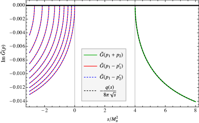
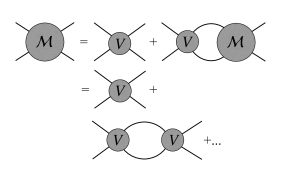
Figure 10: Left: Imaginary part of one loop diagrams appearing in the next-to-leading scattering amplitude in the $\phi^{4}$ theory. Notably, the $t$ and $u$ channel contributions (different lines correspond to variation of the angle between in- and outgoing momenta) lead to an imaginary part solely in the unphysical region. Right: diagrammatic representation of a unitary scattering amplitude (4.39).

The opening of the imaginary part for negative values of $s$ is what leads to the so-called left-hand cut of the complex $s$-plane. Taking a closer look on the expansion in section 4.5.1 one realizes that

$$\mathcal{M}_{2}-\mathcal{M}_{2}^{*}=-|\mathcal{M}_{1}|^{2}\underbrace{(\tilde{G}(s)-\tilde{G}^{*}(s))}_{=-({2q(s)})/({8\pi\sqrt{s}})}\,,$$ (4.38)

while unitarity, Eq. (2.7), for the unprojected matrix elements yields ${\rm Im}~{}\mathcal{M}=\frac{q(s)}{8\pi\sqrt{s}}|\mathcal{M}|^{2}$, meaning that the unitarity condition is fulfilled perturbatively only. In general, restoration of unitarity to all orders is what is referred to as unitarization. Various ways exist in this regard, some of most popular ones will be discussed below.

A large class of approaches starts from the following general ansatz

$$\mathcal{M}(p_{1}^{\prime},p_{1};p)=V(p_{1}^{\prime},p_{1};p)-\int\frac{d^{d}k}{(2\pi)^{d}}V(p_{1}^{\prime},k;p)G(k;p)\mathcal{M}(k,p_{1};p)\,,$$ (4.39)

in terms of a two-body propagator $G$ and an interaction kernel $V$. Of course, regularization of the integral equation is understood. Indeed, the form of the two-body propagator $G$ is what defines the specific ansatz, which for the Bethe-Salpeter equation (BSE) and scalar particles reads $G(k;p)=\mathrm{i}/(k^{2}-M^{2}+\mathrm{i}\epsilon)/((p-k)^{2}-M^{2}+\mathrm{i}\epsilon)$. The interaction is encoded in the kernel $V(p^{\prime},p;p)$, which is typically derived from an effective field theory.

Eq. (4.39) is a genuine $d$-dimensional integral equation which can be interpreted as an infinite series of Feynman diagrams, see the right panel of Fig. 10. In general, such an equation cannot be solved analytically, but examples exists where this has been performed [256, 257, 258, 259, 260, 261, 262]. One simplification can be achieved by assuming that neither $\mathcal{M}$ nor the interaction kernel $V$ have singularities in $k^{0}$, allowing to perform the $k^{0}$ integral using Cauchy’s theorem. This reduces the dimension of the integral, effectively putting the intermediate particles on the mass-shell $k^{2}=M^{2}$. While this destroys manifest covariance, the resulting equation is still covariant. It is often referred to as the quasipotential or Gross equation, see, e.g., Ref. [263]. Still, the equation keeps its genuine integral form. Simplifying this further, one assumes often a projection of the interaction kernel $V$ (on-shell) onto a partial wave of interest (most of the S-wave). Such a projected potential $\tilde{V}_{\ell}$ can only depend on the total energy squared $s$, such that the integral equation above indeed becomes an algebraic one with the solution

$$\mathcal{M}_{\ell}(s)=\tilde{V}_{\ell}(s)-\tilde{V}_{\ell}\tilde{G}(s)\mathcal{M}_{\ell}(s)=\frac{1}{1+\tilde{V}_{\ell}(s)\tilde{G}(s)}\tilde{V}_{\ell}(s)\,.$$ (4.40)

For our example of the $\phi^{4}$ theory with $\tilde{V}(s)=-\lambda$, so that Eq. (4.40) indeed is also the solution of the BSE (4.39). For a general theory this solution is referred most-commonly to as unitarized scattering amplitude.

So far, we have seen that the Bethe-Salpeter equation (4.39) allows to restore unitarity, keeping close connection to the Feynman diagrams. While in general this equation is hard to solve, it can be reduced to an algebraic one projecting the interaction kernel to a specific (on-shell) partial wave. Obviously, this still preserves unitarity since ${\rm Im}~{}\mathcal{M}_{\ell}^{-1}(s)=-q(s)/(8\pi\sqrt{s})$ as demanded by Eq. (2.8), bringing this ansatz close to the general K-matrix form discussed in Sec. 2. Specifically, matching Eq. (2.9) with Eq. (4.40) relates

$$K_{\ell}^{-1}(s)=\tilde{V}_{\ell}^{-1}(s)+{\rm Re}~{}\tilde{G}(s)\,.$$ (4.41)

Over the last decades, the BSE in integral and algebraic form has become a workhorse for many investigations of, e.g., resonant dynamics of two-hadron scattering in the non-perturbative regime of QCD. Deriving the interaction kernel from some effective field theory, predictions on the resonance structure on the Riemann-sheets can be made. However, there is a price to the flexibility and simplicity of this approach as the crossing symmetry does no longer hold. Note that approaches to the restoration of crossing symmetry in this context have been formulated, see, e.g., Refs. [264, 215]. In general the fact that crossing symmetry is violated, and only a subset of all possible Feynman diagrams can be considered by the above unitarization technique yields that standard renormalization methodology cannot be applied. Indeed, the scattering amplitude eq. 4.40 remains explicitly dependent on the regularization scale. This means that when fitting two different versions of a unitarized amplitude to the same data using the same interaction kernel leads to different parameters and predictions outside of fitting region. This means that such an unitarization procedure inevitably induces some model-dependence.

4.5.2 Light quark sector: Meson-meson scattering

The application of the BSE methodology to the light (up and down) quark sector have been plentiful both in the meson [265, 266, 267] as well as baryon sector [268, 260, 269], which also includes extensions to coupled channels. Pertinent works including also the strange and the heavy quarks will be discussed below.

Many other unitarization techniques have been developed to address the lowest mesonic resonances. The $N/D$ approach [270] derives from dispersion relations and includes in principle both the left-hand cuts (in $N$) and unitarity right-hand cut (in $D$), see fig. 10. In particular, the amplitude is written as

$$\mathcal{M}_{N/D}(s)=\frac{N(s)}{D(s)}\,.$$ (4.42)

After this definition, an ansatz is made for the numerator $N^{I\ell}(s)$, which typically stems from the perturbative expansion of effective field theories or more general functions with constraints from the behavior of partial waves near threshold [271]. Finally, one can deduce the denominator from the unitarity condition, $Im~{}D(s)=-N(s)\theta(s-s_{\rm thr})$ rescaled appropriately, with $s_{\rm thr}$ the physical two-body threshold. This is done by means of a dispersion relation with respect to Mandelstam $s$ including an appropriate number of subtractions. These subtractions are then obtained from fits to data. For applications to $\pi\pi$ and $\pi N$ scattering see, Refs [271, 272, 273] and [274], respectively. For recent work on other hadron-hadron scattering processes using the $N/D$ method, see e.g. Refs. [275, 276, 277, 278].

Another very popular approach is the so-called inverse amplitude method (IAM) [163, 279, 280, 281]. Also here in addition to unitarity the left-hand cut is included at least perturbatively. This is because the amplitude matches the chiral amplitude up to the next-to-leading order which also makes the approach an ideal tool to access universal parameters of, e.g., the $f_{0}(500)$ and $\rho(770)$ resonances from phenomenology [46, 44, 282] and lattice QCD [108, 41, 283] (at unphysical pion masses). As it turns out, the same amplitude also fulfills the general requirements on the chiral trajectory of resonances to all chiral orders [255].

Specifically, the partial wave amplitude projected to isospin $I$ and angular momentum $\ell$ reads

$$\mathcal{M}_{\rm IAM}^{I\ell}(s)=\frac{(\mathcal{M}_{2}^{I\ell}(s))^{2}}{\mathcal{M}_{2}^{I\ell}(s)-\mathcal{M}_{4}^{I\ell}(s)}\,,$$ (4.43)

where $\mathcal{M}_{n}^{I\ell}(s)$ denotes the $n$th order chiral amplitudes [137, 138]. The leading order chiral amplitude ($\mathcal{M}_{2}^{I\ell}(s)$) is a function of energy, Goldstone-boson mass, $M^{2}=B(m_{u}+m_{d})$ and pion decay constant in the chiral limit, $F$. The next-to-leading order amplitude ($\mathcal{M}_{4}^{I\ell}(s)$) involves in the two-flavor case two low-energy constants (LECs) $\bar{l}_{1}$ and $\bar{l}_{2}$. Two additional low-energy constants $\bar{l}_{3}$, $\bar{l}_{4}$ enter the NLO chiral amplitude when replacing the above mass and decay constants by their physical values using the well-known one-loop results [137],

$$M_{\pi}^{2}=M^{2}\left(1-\frac{M^{2}}{32\pi^{2}F^{2}}\bar{l}_{3}\right)\,,\qquad F_{\pi}=F\left(1+\frac{M^{2}}{16\pi^{2}F^{2}}\bar{l}_{4}\right)\,.$$ (4.44)

By construction, the LECs $\bar{l}_{i}$ do not depend on the regularization scale. Because of that, they acquire a dependence on the quark masses. This is of course disadvantageous when studying results of lattice calculations performed at unphysical pion masses, but can be overcome by using the more conventional scale-dependent but quark-mass-independent renormalized LECs $l_{i}^{r}$. The relation between two reads

$$l_{i}^{r}=\frac{\gamma_{i}}{32\pi^{2}}\left(\bar{l}_{i}+\log\frac{M^{2}}{\mu^{2}}\right)\,,$$ (4.45)

where $\gamma_{1}=1/3$, $\gamma_{2}=2/3$, $\gamma_{3}=-1/2$, $\gamma_{4}=2$. Hence, for a fixed scale $\mu$ one can determine the renormalized LECs and then make predictions for two-particle scattering at a different pion mass. We note that fixing $\mu$ in physical units may lead to subtleties when addressing scale-independent quantities in lattice QCD. However, in some cases methods exists to overcome this issue, see discussions in Refs. [284, 285, 108].

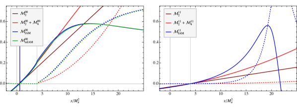
Figure 11: Comparison between the perturbative chiral amplitudes with the inverse amplitude method Eq. (4.43) for the isoscalar and isovector $\pi\pi$ channels. Full and dashed lines denote real and imaginary (if existing) parts, respectively. In the isoscalar case the chiral amplitude is vanishing exactly at $s\approx 1/2M_{\pi}^{2}$ (the Adler zero). This yields a pole in the IAM approach, which is removed by following the modified inverse amplitude method Eq. (4.5.2), see text for mode details.

In the past, the IAM was used successfully to gain deeper insights into the long-debated $f_{0}(500)$ isoscalar $\pi\pi$ resonance, see the dedicated review [44]. In this context we show a comparison of the perturbative chiral amplitude with the IAM scattering amplitude in fig. 11 for isovector and isoscalar scattering. Using LECs from a perturbative analysis [137] for demonstration only, we observe that the unitarized amplitude $\mathcal{M}_{\rm IAM}$, indeed, is close to the next-to-leading order chiral amplitude close to the threshold but exhibits a resonant behavior at $\sqrt{s}\approx 500~{}{\rm MeV}$ and $\sqrt{s}\approx 770~{}{\rm MeV}$, respectively, in the isoscalar and isovector channel. In the former case we observe additionally that the perturbative amplitude vanishes exactly at $s\approx 2M_{\pi}^{2}$, the Adler zero [286]. This leads to the fact that around this energy also the denominator of $\mathcal{M}_{\rm IAM}$ vanishes. Notably, the same happens for the case of maximal isospin ($\mathcal{M}_{2}^{20}$) at $s\approx 2M_{\pi}^{2}$. Obviously, this singularity has very small residuum, such that for studies of experimental data, this effect is negligible. Still from the conceptual point of view as well when embedding this two-body model into, e.g., multihadron setting [287, 86] the subthreshold behavior may become important. Fortunately, there is a convenient way to remove this spurious pole by a procedure established in, e.g., Refs. [288, 46].

$$\mathcal{M}_{\rm IAM}^{I\ell}(s)\longrightarrow\mathcal{M}_{\rm mIAM}^{I\ell}(s) =\frac{(\mathcal{M}_{2}^{I\ell}(s))^{2}}{\mathcal{M}_{2}^{I\ell}(s)-\mathcal{M}_{4}^{I\ell}(s)+A^{I\ell}_{m}(s)}\,,$$

$$A^{I\ell}_{m}(s) =\mathcal{M}_{4}^{I\ell}(s_{2})-\frac{(s_{2}-s_{A})(s-s_{2})\left(\mathcal{M}_{2}^{I\ell\prime}(s_{2})-\mathcal{M}_{4}^{I\ell\prime}(s_{2})\right)}{s-s_{A}}\,,$$ (4.46)

where $s_{A}$ and $s_{2}$ are the zeros of $\mathcal{M}_{2}^{I\ell}(s)-\mathcal{M}_{4}^{I\ell}(s)$ and $\mathcal{M}_{2}^{I\ell}(s)$, respectively. In this form the inverse amplitude method has been applied frequently [46, 289, 290, 43], simultaneously describing all three $\pi\pi$ isospin channels, and making, e.g., predictions for the quark mass dependence of the light-quark resonance parameters, see fig. 4 and discussion thereof.

4.5.3 Light quark sector: Meson-baryon sector

The principle of dynamical generation of resonances has helped to understand many low-lying states in the hadron spectrum. Including the strange quark enriches this picture even more. This is because production thresholds are separated stronger than in the light ($u,d$) sector. Arguably the most prominent examples in this sense is the the long-debated $\Lambda(1405)$ resonance, which indeed is dynamically generated due to strong attraction of $\bar{K}N$ and interference with the $\pi\Sigma$ channels. Several reviews [291, 292, 293, 294] have been dedicated to the history and state of the art understanding of this enigmatic state. Thus, we will only mention facts relevant for this review, referring the reader for more details to the quoted reviews.

The current method of choice in the studies of antikaon-nucleon scattering is based on the already discussed Bethe-Salpeter equation. In that, the interaction kernel is taken from the chiral meson-baryon Lagrangian at next-to-leading order, which in its full form reads

$$V_{\rm off}(\not{q^{\prime}},\not{q};P)= \Bigg{(}A_{WT}(\not{q}+\not{q^{\prime}})+A_{Bs}\not{q^{\prime}}\frac{m-\not{P}}{s-m^{2}}\not{q}+A_{Bu}\not{q}\frac{m-\not{P}+\not{q^{\prime}}+\not{q}}{u-m^{2}}\not{q^{\prime}}\Bigg{)}_{\rm LO}+$$ (4.47)

$$\Bigg{(}A_{14}(q\cdot q^{\prime})+A_{57}[\not{q},\not{q^{\prime}}]+A_{M}+A_{811}\left(\not{q^{\prime}}\left(q\cdot P)+\not{q}(q^{\prime}\cdot P\right)\right)\Bigg{)}_{\rm NLO}\,,$$

where $P=p+q=p^{\prime}+q^{\prime}$, and $s=P^{2}$, $u=(p-q^{\prime})^{2}$ are the usual Mandelstam variables. We note that 10 combinations of ground state octet mesons and baryons have the same quantum numbers, i.e., $\{K^{-}p$, $\bar{K}^{0}n$, $\pi^{0}\Lambda$, $\pi^{0}\Sigma^{0}$, $\pi^{+}\Sigma^{-}$, $\pi^{-}\Sigma^{+}$, $\eta\Lambda$, $\eta\Sigma^{0}$, $K^{+}\Xi^{-}$, $K^{0}\Xi^{0}\}$ meaning that the scattering amplitude $\mathcal{M}$ must describe the dynamics of all coupled-channels simultaneously. Thus, the interaction kernel $V$ is a $10\times 10$ matrix build from the matrices $A_{...}$. These depend explicitly on the meson decay constants and axial couplings $D$, $F$ at leading, and on the LECs $\{b_{0},b_{D},b_{F},b_{1},...,b_{11}\}$ at next-to-leading chiral order. This already demonstrates the rapid rise of the number of unknown LECs as well as momentum structures compared to, e.g., light-quark $(u,d)$ meson sector (4 LECs). Also, the higher dimension of the kernel increases the computational costs strongly. However, as discussed before, various approximations and simplifications can be applied to the above kernel. For example off-shell effects appear to be rather small as studied in Ref. [295]. Also, it seems safe to assume that NLO terms are required to produce realistic scattering amplitudes.

Ultimately, various approximations and unitarization variations lead consistently to a narrow pole close to the $\bar{K}N$ threshold, additionally predicting a second lighter and broader pole, when using similar experimental data for fits of the free parameters. As we know now, see the recent review [292], such unusual double pole structures are not uncommon in many other parts of the hadronic spectrum.

4.5.4 Heavy-light quark sector: Goldstone bosons scattering off $D$ mesons

Unitarization methods are also successfully used in the coupled-channel scattering of Goldstone bosons off ($\pi,K,\eta$) $D$ (and $D^{*}$) mesons, which allows to dynamically generate the mysterious charmed scalar mesons, in particular the charm-scalar mesons [296, 297, 298] that showed that the conventional quark model was insufficient. There were considered early as hadronic molecules in a theory combining chiral and heavy quark symmetry [299, 264] or within the chiral doubling approach [300], see also the reviews [8, 16, 301]. A further important observation was the two-pole structure of the $D_{0}^{*}(2300)$ [302] that was first worked out explicitly in the analysis of lattice QCD data on heavy-light pseudoscalar meson $J^{P}=0^{+}$ scattering in the strangeness-isospin $(S,I)=(0,1/2)$ sector from the Hadron Spectrum Collaboration [303]. This had been noted before but was not out into proper context [264, 304, 305]. Combining unitarized perturbation theory in the heavy-light sector with data from lattice QCD and also from the LHCb collaboration on $B\to D\pi\pi$ decays [306, 307, 308, 309]. finally led to a new paradigm for heavy-light spectroscopy [310] and further helped to establish the two-pole structure as more general phenomenon in the hadron spectrum rather than being a curiosity related to the enigmatic $\Lambda(1405)$ [292] as discussed in more detail in section 6. Note that the type of three-body decays $B\to D\pi\pi$ requires a different effective Lagrangian than the one used for $D\phi$ scattering, as will also be discussed below.

First, let us recall the power counting for Goldstone boson scattering off matter fields, here the triplet of $D$ (and $D^{*}$) mesons. To be specific, we consider the EOMS scheme. External momenta as well as the masses of the Goldstone bosons are counted as ${\cal O}(p)$, where $p$ denotes a small quantity. However, the nonvanishing masses of the $D$ and $D^{*}$ in the chiral limit introduce new scales $M_{0}$ and $M_{0}^{*}$, both counted as ${\cal O}(1)$. As a result, at low energies, the temporal components of the momenta of the $D$ and $D^{*}$ are counted as ${\cal O}(1)$, while the spatial components are counted as ${\cal O}(p)$. Therefore, the virtuality $q^{2}-M_{0}^{(*)2}$ in the propagators scales as ${\cal O}(p)$, and the propagators scale as ${\cal O}(p^{-1})$. The Goldstone boson propagators are counted as ${\cal O}(p^{-2})$ as usual. In the EOMS scheme, the power counting breaking terms are absorbed into the redefinition of the LECs so that the resulting physical observables obey the power counting rules. This is explicitly worked out in Ref. [311]. Most calculation of the scattering potentials have been carried out to NLO, but there are a few works that attempted an NNLO calculation.

The effective Lagrangian for the calculation of the unitarized $D\phi$ scattering amplitudes up to leading one-loop order can be written as

$$\mathcal{L}_{\rm eff}=\sum_{i=1}^{2}\mathcal{L}_{\phi\phi}^{(2i)}+\sum_{j=1}^{3}\mathcal{L}_{D\phi}^{(j)}+\sum_{k=1}^{2}\mathcal{L}_{D^{\ast}\phi}^{(k)}+\sum_{l=1}^{3}\mathcal{L}_{D^{\ast}D\phi}^{(l)}\,,$$ (4.48)

with the superscripts specifying the chiral dimension. The terms in the Goldstone sector are the standard ones [138] and the terms corresponding to interactions between the $D=(D^{0},D^{+},D_{s}^{+})$ mesons and the Goldstone bosons are given by [312, 313, 314, 315, 316, 317]

$$\mathcal{L}^{(1)}_{D\phi} = \mathcal{D}_{\mu}D\mathcal{D}^{\mu}D^{\dagger}-{M}_{0}^{2}DD^{\dagger}\ ,$$

$$\mathcal{L}^{(2)}_{D\phi} = D\left(-h_{0}\langle\chi_{+}\rangle-h_{1}{\chi}_{+}+h_{2}\langle u_{\mu}u^{\mu}\rangle-h_{3}u_{\mu}u^{\mu}\right){D}^{\dagger}+\mathcal{D}_{\mu}D\left({h_{4}}\langle u_{\mu}u^{\nu}\rangle-{h_{5}}\{u^{\mu},u^{\nu}\}\right)\mathcal{D}_{\nu}{D}^{\dagger}\,,$$ (4.49)

$$\mathcal{L}^{(3)}_{D\phi} = D\biggl{[}\mathrm{i}\,{g_{1}}[{\chi}_{-},u_{\nu}]+{g_{2}}\left([u_{\mu},[\mathcal{D}_{\nu},u^{\mu}]]+[u_{\mu},[\mathcal{D}^{\mu},u_{\nu}]]\right)\biggr{]}\mathcal{D}^{\nu}{D}^{\dagger}+g_{3}D\,[u_{\mu},[\mathcal{D}_{\nu},u_{\rho}]]\mathcal{D}^{\mu\nu\rho}{D}^{\dagger}\ +h.c.\,,$$

where $M_{0}$ is the $D$ meson mass in the chiral limit, the $h_{i}$ and $g_{j}$ are LECs and the chiral building blocks are given as above $u_{\mu}=\mathrm{i}[u^{\dagger}\partial_{\mu}u-u\partial_{\mu}u^{\dagger}]$, $U=u^{2}$ and $\chi^{\pm}=u^{\dagger}\chi u^{\dagger}\pm u\chi^{\dagger}u$. The covariant derivative is defined via

$$\mathcal{D}_{\mu}H=H(\overset{\leftarrow}{\partial_{\mu}}+\Gamma_{\mu}^{\dagger})\ ,\qquad\mathcal{D}_{\mu}H^{\dagger}=(\partial_{\mu}+\Gamma_{\mu})H^{\dagger}\ ,$$ (4.50)

and $\mathcal{D}^{\mu\nu\rho}=\{\mathcal{D}_{\mu},\{\mathcal{D}_{\nu},\mathcal{D}_{\rho}\}\}$, where $H\in\{D,D^{\ast}\}$ with $D^{\ast}=(D^{\ast 0},D^{\ast+},D_{s}^{\ast+})$. The so-called chiral connection in the covariant derivatives is defined as $\Gamma_{\mu}=\left(u^{\dagger}\partial_{\mu}u+u\partial_{\mu}u^{\dagger}\right)/2.$ Similarly, the relevant terms for the interaction between the $D^{\ast}$ and the Goldstone bosons are [312, 313, 314]

$$\mathcal{L}_{D^{\ast}\phi}^{(1)}=-\frac{1}{2}\mathcal{F}^{\mu\nu}\mathcal{F}_{\mu\nu}^{\dagger}+M_{0}^{\ast 2}D^{\ast\nu}D^{\ast\dagger}_{\nu}\,,~{}~{}~{}\mathcal{L}_{D^{\ast}\phi}^{(2)}=\ D_{\mu}^{\ast}\left[\tilde{h}_{0}\langle\chi_{+}\rangle+\tilde{h}_{1}{\chi}_{+}\right]D^{\mu\ast\dagger}\ ,$$ (4.51)

with $\tilde{h}_{0,1}$ analogous to $h_{0,1}$ and $\mathcal{F}_{\mu\nu}=(\mathcal{D}_{\mu}D^{\ast}_{\nu}-\mathcal{D}_{\nu}D^{\ast}_{\mu})$. In the heavy quark limit, $\tilde{h}_{0}=h_{0}$ and $\tilde{h}_{1}=h_{1}$. Note that due to the trace structure in the corresponding operator, the LECs $h_{0}$, $h_{2}$ and $h_{4}$ are suppressed in the large-$N_{c}$ limit [318]. The LEC $h_{1}$ can be deduced from the mass splittings in the $D$ meson triplet,

$$h_{1}=\frac{M_{D_{s}}^{2}-M_{D}^{2}}{4(M_{K}^{2}-M_{\pi}^{2})}=0.427\,.$$ (4.52)

The quark mass dependence of $M_{D}$ and $M_{D_{s}}$ fixes $h_{0}\simeq 0.01$, which is consistent with the expectations from large-$N_{c}$. The other LEC are determined from fits to lattice QCD data, see below. Finally, the LO axial coupling has the form

$$\mathcal{L}_{D^{\ast}D\phi}^{(1)}=\mathrm{i}\,{g_{0}}\left(D^{\ast}_{\mu}u^{\mu}D^{\dagger}-D\,u^{\mu}D^{\ast\dagger}_{\mu}\right)\ .$$ (4.53)

As pointed out in Refs. [243, 244], the resonance-exchange contributions of $\mathcal{O}(p^{2})$ and $\mathcal{O}(p^{3})$ can be taken into account by shifting the coupling in the LO resonance-exchange contribution and the LECs in the contact terms. This also holds true for our case. Thus, we do not need the ${\cal O}(p^{2})$ and ${\cal O}(p^{3})$ terms for the $D^{\ast}D\phi$ coupling. The $DD^{*}\pi$ axial coupling constant $g_{0}$ can be fixed by the decay width $\Gamma(D^{*+}\to D^{0}\pi^{+})$. As discussed in Refs. [316], one gets $g=(1.11\pm 0.15)~{}\text{GeV}$ for the renormalized coupling $g$, which contains the bare constants $g_{0}$ and one-loop chiral corrections.

$(S,I)$	Channels	$C_{\rm LO}$	$C_{0}$	$C_{1}$	$C_{24}$	$C_{35}$
$(-1,0)$	$D\bar{K}\to D\bar{K}$	$-1$	$M_{K}^{2}$	$M_{K}^{2}$	1	$-1$
$(-1,1)$	$D\bar{K}\to D\bar{K}$	1	$M_{K}^{2}$	$-M_{K}^{2}$	1	1
$(2,\frac{1}{2})$	$D_{s}K\to D_{s}K$	1	$M_{K}^{2}$	$-M_{K}^{2}$	1	1
$(0,\frac{3}{2})$	$D\pi\to D\pi$	1	$M_{\pi}^{2}$	$-M_{\pi}^{2}$	1	1
$(1,1)$	$D_{s}\pi\to D_{s}\pi$	0	$M_{\pi}^{2}$	0	1	0
	$DK\to DK$	0	$M_{K}^{2}$	0	1	0
	$DK\to D_{s}\pi$	1	0	$-(M_{K}^{2}+M_{\pi}^{2})/2$	0	1
$(1,0)$	$DK\to DK$	$-2$	$M_{K}^{2}$	$-2M_{K}^{2}$	1	2
	$D_{s}\eta\to D_{s}\eta$	0	$M_{\eta}^{2}$	$-2M_{\eta}^{2}+2M_{\pi}^{2}/3$	1	$4/3$
	$DK\to D_{s}\eta$	$-\sqrt{3}$	0	$-\sqrt{3}(5M_{K}^{2}-3M_{\pi}^{2})/6$	0	$1/{\sqrt{3}}$
$(0,\frac{1}{2})$	$D\pi\to D\pi$	$-2$	$M_{\pi}^{2}$	$-M_{\pi}^{2}$	1	1
	$D\eta\to D\eta$	0	$M_{\eta}^{2}$	$-M_{\pi}^{2}/3$	1	$1/3$
	$D_{s}\bar{K}\to D_{s}\bar{K}$	$-1$	$M_{K}^{2}$	$-M_{K}^{2}$	1	1
	$D\eta\to D\pi$	0	0	$-M_{\pi}^{2}$	0	1
	$D_{s}\bar{K}\to D\pi$	$-{\sqrt{6}}/{2}$	0	$-{\sqrt{6}}(M_{K}^{2}+M_{\pi}^{2})/4$	0	${\sqrt{6}}/{2}$
	$D_{s}\bar{K}\to D\eta$	$-{\sqrt{6}}/{2}$	0	${\sqrt{6}}(5M_{K}^{2}-3M_{\pi}^{2})/12$	0	$-1/{\sqrt{6}}$

Table 1: The coefficients in the scattering amplitudes $V(s,t,u)$. The channels are labelled by strangeness ($S$) and isospin ($I$).

Consider now the scattering process $D_{1}(p_{1})\phi_{1}(p_{2})\to D_{2}(p_{3})\phi_{2}(p_{4})$ in more detail. There are alltogether 16 channels with different total strangeness $S$ and isospin $I$ as listed in table 1, see, e.g., Refs. [304, 319, 320, 315, 305, 321, 322, 323, 324, 325, 316, 326, 327, 328, 310, 329]. Using the NLO chiral Lagrangian from Ref. [315], the scattering amplitudes are given by

$$V(s,t,u)=\frac{1}{F_{0}^{2}}\bigg{[}\frac{C_{\rm LO}}{4}(s-u)-4C_{0}h_{0}+2C_{1}h_{1}-2C_{24}H_{24}(s,t,u)+2C_{35}H_{35}(s,t,u)\bigg{]}\,,$$ (4.54)

where $F_{0}$ is the pion decay constant in the chiral limit, and the coefficients $C_{i}$ can be found in Tab. 1. Further,

$$H_{24}(s,t,u) = 2h_{2}p_{2}\cdot p_{4}+h_{4}(p_{1}\cdot p_{2}p_{3}\cdot p_{4}+p_{1}\cdot p_{4}p_{2}\cdot p_{3})\,,$$

$$H_{35}(s,t,u) = h_{3}p_{2}\cdot p_{4}+h_{5}(p_{1}\cdot p_{2}p_{3}\cdot p_{4}+p_{1}\cdot p_{4}p_{2}\cdot p_{3})\,.$$ (4.55)

For NNLO corrections and contributions from the $D^{*}$ mesons, see, e.g., Ref. [328]. The appearing LECs can be determined from a fit to lattice data. In order to reduce the correlations between the LECs, one introduces the following redefinitions of the LECs [323, 316]

$$h_{4}^{\prime} = h_{4}\bar{M}_{D}^{2}\,,\quad h_{5}^{\prime}=h_{5}\bar{M}_{D}^{2}\,,\quad h_{24}=h_{2}+h_{4}^{\prime}\,,\quad h_{35}=h_{3}+2h_{5}^{\prime}\,,$$

$$g_{1}^{\prime} = g_{1}\bar{M}_{D}\,,\quad g_{2}^{\prime}=g_{2}\bar{M}_{D}\,,\quad g_{3}^{\prime}=g_{3}\bar{M}_{D}^{3}\,,\quad g_{23}=g_{2}^{\prime}-2g_{3}^{\prime}\,,$$ (4.56)

where $\bar{M}_{D}$ is the average of the physical masses of the charmed mesons $D$ and $D_{s}$, $\bar{M}_{D}=(M_{D}^{\text{Phy}}+M_{D_{s}}^{\text{Phy}})/2$. The new LECs $h_{4}^{\prime}$, $h_{5}^{\prime}$, $h_{24}$ and $h_{35}$ are dimensionless, and $g_{1}^{\prime}$, $g_{3}^{\prime}$ and $g_{23}$ have the dimension of inverse mass.

Before unitarization, a partial wave projection to a definite orbital angular momentum $\ell$ should be performed

$${V}_{\ell}^{(S,I)}(s)_{D_{1}\phi_{1}\to D_{2}\phi_{2}}=\frac{1}{2}\int_{-1}^{+1}{\rm d}\cos\theta\,P_{\ell}(\cos\theta)\,{V}^{(S,I)}_{D_{1}\phi_{1}\to D_{2}\phi_{2}}(s,t(s,\cos\theta))\,,$$ (4.57)

where $\theta$ is the scattering angle between the incoming and outgoing particles in the center-of-mass frame, and the Mandelstam variable $t$ is expressed as

$$t(s,\cos\theta)=M_{D_{1}}^{2}+M_{D_{2}}^{2}-\frac{\left(s+M_{D_{1}}^{2}-M_{\phi_{1}}^{2}\right)\left(s+M_{D_{2}}^{2}-M_{\phi_{2}}^{2}\right)}{2s}-\frac{\cos\theta}{2s}\sqrt{\lambda(s,M_{D_{1}}^{2},M_{\phi_{1}}^{2})\lambda(s,M_{D_{2}}^{2},M_{\phi_{2}}^{2})}\,,$$ (4.58)

where $\lambda(a,b,c)=a^{2}+b^{2}+c^{2}-2ab-2ac-2bc$ is the Källén function. In most cases, one considers S-wave scattering, and, thus, the subscript $\ell=0$ is dropped.

At this point, it is worth to discuss some problems arising in such unitarization procedures. It is well-known that any unitarization approach that relies on right-hand unitarity and the on-shell approximation has the problem of violation of unitarity when the left-hand cut occurs in the on-shell potential. For instance, the left-hand cut in the $K\bar{K}\to K\bar{K}$ amplitude leads a violation of unitarity for the $\pi\pi$ scattering in the $\pi\pi$–$K\bar{K}$ coupled-channel system [330, 331]. Note, however, that it was shown in Refs. [332, 330] that the unitarity violation is numerically small in the $\pi\pi$-$K\bar{K}$ case, thus, no serious problem is generated. The same unitarity violation happens to the $D\phi$ scattering with $(S,I)=(0,1/2)$, which has three coupled channels: $D\pi$, $D\eta$ and $D_{s}\bar{K}$. One of the left-hand cuts from the inelastic channel $D_{s}\bar{K}\to D\eta$ amplitude, from ($1.488$ GeV)² to ($2.318$ GeV)², overlaps with the right-hand cut starting from the $D\pi$ threshold. Although this left-hand cut is not numerically important, its presence together with other left-hand cuts and right-hand cuts make the whole real axis nonanalytic. As a result, the coupled-channel amplitudes do not have the correct analytic properties even in the relevant energy region. Consequently, a pair of pole at $(2.046\pm i0.050)~{}\text{GeV}$ are found on the first Riemann sheet for the coupled-channel $(S,I)=(0,1/2)$ amplitude. As we know, poles on the first Riemann sheet can only be located on the real axis below the lowest threshold, which are associated with bound states. A pole on the first sheet with a non vanishing imaginary part or above the lowest threshold is inconsistent with causality. The appearance of the pole on the first sheet in the coupled-channel $(S,I)=(0,1/2)$ is due to the existence of the coupled-channel cut. The left-hand cuts stem from the one-loop potentials but only at NNLO. If one considers only a single-channel such as $D\pi\to D\pi$ with $(S,I)=(0,1/2)$, there is no such problem as it comes from the left-hand cut of the inelastic channels.

Finally, we consider $D\phi$ scattering as a sub-process of the weak decays $B\to D\phi\phi$. At low energies, for the processes with $\Delta b=1$ and $\Delta c=1$ the interaction can be described by the effective weak Hamiltonian $H_{\text{eff}}$ which at LO has the form [333]

$$H_{\text{eff}}=\frac{G_{F}}{\sqrt{2}}V_{cb}^{\ast}V_{ud}\big{(}C_{1}\mathcal{O}^{d}_{1}+C_{2}\mathcal{O}^{d}_{2}\big{)}+(b\to s)+\text{h.c.}\,,$$ (4.59)

with $G_{F}$ the Fermi constant, $V_{ij}$ the Cabibbo–Kobayash–Maskawa (CKM) matrix elements, and the $C_{i}$ are scale-dependent Wilson coefficients. Here, the tree-level operators read

$$\mathcal{O}^{d}_{1}=(\bar{c}_{a}b_{b})_{L}(\bar{d}_{b}u_{a})_{L}\,,~{}~{}~{}\mathcal{O}^{d}_{2}=(\bar{c}_{a}b_{a})_{L}(\bar{d}_{b}u_{b})_{L}\,,$$ (4.60)

with the subscripts $a$ and $b$ are color indices. The subscript $L$ indicates that only the left-hand components of the quarks are involved. Note that here the color space is irrelevant for our discussion, thus, we simply drop the subscripts of $C_{i}$ and $\mathcal{O}_{i}$ hereafter. One can make the effective Hamiltonian fully chirally invariant by introducing a spurion $H_{i}^{j}$ transforming as [334]

$$H_{i}^{j}\mapsto H_{i^{\prime}}^{j^{\prime}}(g_{L})_{i}^{i^{\prime}}(g_{L}^{\dagger})_{j^{\prime}}^{j}\,.$$ (4.61)

Then the new Hamiltonian

$$H_{\text{eff}}^{\prime}=\frac{G_{F}}{\sqrt{2}}V_{cb}^{\ast}V_{ud}H_{i}^{j}C(\bar{c}b)_{L}(\bar{q}_{L}^{i}q_{Lj})$$ (4.62)

is chirally invariant. For Eq. (4.59), the spurion $H_{i}^{j}$ (the lower index labels rows and the upper one labels columns) corresponds to

$$H=\begin{pmatrix}0&0&0\\ 1&0&0\\ V_{us}/V_{ud}&0&0\end{pmatrix}~{}.$$ (4.63)

Here, $V_{us}/V_{ud}$ is nothing but $-\sin\theta_{1}$, with $\theta_{1}$ the Cabbibo angle. Then the component $H_{2}^{1}$ describes the Cabibbo-allowed decays and $H_{3}^{1}$ the Cabibbo-suppressed ones. In the matrix form, $H$ transforms under chiral symmetry as $H\mapsto g_{L}Hg_{L}^{\dagger}$. It is more convenient to introduce a homogeneously transforming suprion as $t=uHu^{\dagger}$. With those ingredients, one constructs the effective Lagrangian describing the three-body nonleptonic decays of $B$ mesons to $D$ mesons and two light pseudoscalars. We are interested in the region of the invariant mass of a pair of the $D$ and one pseudoscalar not far from their threshold, such that this light pseudoscalar can be safely treated as a soft Goldstone boson, while the other one moves fast and can be treated as a matter field rather than a Goldstone boson. The fast moving pseudoscalar is realized linearly in a matrix form $M$ transforming as

$$M\mapsto hMh^{\dagger}~{},$$ (4.64)

and it has the same form as $\phi$, i.e.,

$$M=\begin{pmatrix}\frac{1}{\sqrt{2}}\pi^{0}+\frac{1}{\sqrt{6}}\eta&\pi^{+}&K^{+}\\ \pi^{-}&-\frac{1}{\sqrt{2}}\pi^{0}+\frac{1}{\sqrt{6}}\eta&K^{0}\\ K^{-}&\bar{K}^{0}&-\frac{2}{\sqrt{6}}\eta\end{pmatrix}.$$ (4.65)

Consequently, utilizing the power counting described above, chiral symmetry implies that the effective Lagrangian at $\mathcal{O}(p)$ has the form of [335, 310, 336]

$${\cal L}_{\text{eff}} =\bar{B}\,\Big{[}c_{1}(u_{\mu}tM+Mtu_{\mu})+c_{2}(u_{\mu}M+Mu_{\mu})t+c_{3}t(u_{\mu}M+Mu_{\mu})$$

$$\qquad\qquad+c_{4}(u_{\mu}\langle Mt\rangle+M\langle u_{\mu}t\rangle)+c_{5}t\langle Mu_{\mu}\rangle+c_{6}\langle(Mu_{\mu}+u_{\mu}M)t\rangle\Big{]}\,\nabla^{\mu}D^{\dagger}$$

$$+\bar{B}\,\Big{[}d_{1}(u_{\mu}tM-Mtu_{\mu})+d_{2}(u_{\mu}M-Mu_{\mu})t+d_{3}t(u_{\mu}M-Mu_{\mu})$$

$$\qquad\qquad+d_{4}(u_{\mu}\langle Mt\rangle-M\langle u_{\mu}t\rangle)+d_{6}\langle(Mu_{\mu}-u_{\mu}M)t\rangle\Big{]}\,\nabla^{\mu}D^{\dagger}\,,$$ (4.66)

where $\bar{B}=(B^{-},\bar{B}^{0},\bar{B}^{0}_{s})$, the $c_{i}$ and $d_{i}$ are LECs, and $\langle\dots\rangle$ denotes a trace in the SU(3) flavor space. Note that the momentum operator $\nabla_{\mu}$ in Eq. (4.5.4) is chosen to act on the charmed meson field $D$. It could act on $B$ (or $M$) independently as well. However, in our case, $M_{B}\gg M_{D}+2M_{\pi}$ and $M_{D}\gg M_{\pi}$ imply that they would produce the same structures up to the LO and we can combine them by redefining the LECs in the heavy meson limit. This effective Lagrangian considers both the chiral symmetry and flavor SU(3) constraints (the latter has been considered in Ref. [335]). Finally, we divide the Lagrangaian (4.5.4) into two groups which are symmetric and antisymmetric in the two light pseudoscalars, which correspond to the cases where the relative orbital angular momentum of the light pseudoscalars pair is even and odd, respectively [335]. The nonleptonic $B$-meson three-body decays $B\to D\phi M$, where $M$ denotes the fast moving light pesudoscalar and $\phi$ denotes the soft one, provide access to the $D$-$\phi$ interaction via the final-state interaction in the energy region where the $D\phi$ system is not far from its threshold. Of course, there also final-state interactions between the $D$ and the hard $M$ and between $M$ and $\phi$. These do not produce any nontrivial structure sensitive to the energy variation and thus can encoded into an extra complex factor. The pertinent Feynman diagrams for the decay $B\to D\phi M$ are shown in Fig. 12, where the square denotes the final-state interactions in the $D\phi$ subsystem.

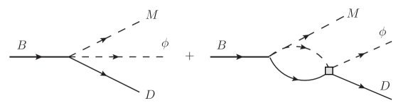
Figure 12: The decay $B\to D\phi M$. The square denotes the final-state interactions between the $D$ meson and the Goldstone boson. In the loop, all relevant coupled channels contribute.

The decay amplitude projected into the $D\phi$ channel at low energies can be decomposed into S-, P- and D-waves, which corresponds to the orbital angular momentum of the $D\phi$ pair $\ell=0$, $\ell=1$, and $\ell=2$, in order,

$$\mathcal{A}(B\to D\phi M)=\mathcal{A}_{0}(s)+\sqrt{3}\mathcal{A}_{1}(s)P_{1}(z)+\sqrt{5}\mathcal{A}_{2}(s)P_{2}(z)\,.$$ (4.67)

Here, $\mathcal{A}_{0,1,2}(s)$ denote the partial wave decomposed amplitudes for $D\phi$ in the S-, P- and D-waves, respectively, and $P_{\ell}(z)$ are the Legendre polynomials with $z$ the cosine of the helicity angle of the $D\phi$ system, i.e., the angle between the moving directions of the $\phi$ and the $M$ in the $D\phi$ rest frame. For the P- and D-waves, the resonances are relatively narrow and, thus, it is reasonable to parameterize them by Breit-Wigner amplitudes. For the S-wave, the diagrams in Fig. 12 are calculated using the effective Lagrangian (4.5.4) and the final-state $D\phi$ interaction is determined from the coupled channels approach described before.

Consider first the decay $B^{-}\to D^{+}\pi^{-}\pi^{-}$. Here, the relative orbital angular momenta of the two light mesons is even. This corresponds to the first term of the Lagrangian in Eq. (4.5.4) parameterized by the LECs $c_{i}$. The corresponding production vertices for the possible intermediate states $D^{0}\pi^{0}$, $D^{+}\pi^{-}$, $D^{0}\eta$ and $D_{s}^{+}K^{-}$ are given in Tab. 2.

$$\begin{array}[]{|c|c|}\hline\cr\text{Process}&\text{Production amplitude}\\ \hline\cr B^{-}\to D^{0}\pi^{0}\pi^{-}&\dfrac{1}{F_{0}}(c_{1}+c_{4})p_{D}\cdot p_{\pi}\\ B^{-}\to D^{0}\eta\pi^{-}&\dfrac{1}{\sqrt{3}F_{0}}(c_{1}+c_{4}+2c_{2}+2c_{6})p_{D}\cdot p_{\eta}\\ B^{-}\to D^{+}\pi^{-}\pi^{-}&\dfrac{2\sqrt{2}}{F_{0}}(c_{1}+c_{4})p_{D}\cdot p_{\pi}\\ B^{-}\to D_{s}^{+}K^{-}\pi^{-}&\dfrac{\sqrt{2}}{F_{0}}(c_{1}+c_{4})p_{D_{s}}\cdot p_{K}\\ \hline\cr\end{array}$$ (4.73)

Table 2: Production vertices for the possible intermediate states contributing to $B^{-}\to D^{+}\pi^{-}\pi^{-}$. The four-momenta of the charmed meson and the Goldstone boson are denoted by $p_{D_{(s)}}$ and $p_{\phi}$, respectively.

In the heavy quark limit, we have $p_{D}\cdot p_{\phi}=M_{D}E_{\phi}$, with $E_{\phi}$ the energy of $\phi$ in the rest frame of the $D\phi$ subsystem. It is convenient to introduce two parameters $A$ and $B$ via [310]

$$A=\frac{\sqrt{2}}{F_{0}}(c_{1}+c_{4})M_{D}~{}\,,~{}~{}~{}B=\frac{2\sqrt{2}}{3F_{0}}(c_{2}+c_{6})M_{D}\,.$$ (4.74)

Consequently, the S-wave decay amplitude for $B^{-}\to D^{+}\pi^{-}\pi^{-}$ that contains the final-state interaction can be written as

$$\mathcal{A}_{0}(s) = 2AE_{\pi}+2AE_{\pi}G_{D\pi}(s)T_{D^{+}\pi^{-}\to D^{+}\pi^{-}}(s)+\frac{A}{\sqrt{2}}E_{\pi}G_{D\pi}(s)T_{D^{0}\pi^{0}\to D^{+}\pi^{-}}(s)$$ (4.75)

$$+\frac{A+3B}{\sqrt{6}}E_{\eta}G_{D\eta}(s)T_{D^{0}\eta\to D^{+}\pi^{-}}(s)+AE_{K}G_{D_{s}\bar{K}}(s)T_{D_{s}^{+}K^{-}\to D^{+}\pi^{-}}(s)\,,$$

with $s$ the center-of-mass energy squared of the $D\phi$ system, and $G_{D\phi}(s)$ is the loop function shown in Fig. 12 coupling to the channel $D\phi$. Unitarity allows to express this loop function via a once-subtracted dispersion relation,

$$G_{D\phi}(s) = \frac{1}{16\pi^{2}}\Bigg{\{}a(\mu)+\log\frac{M_{D}^{2}}{\mu^{2}}+\frac{M_{\phi}^{2}-M_{D}^{2}+s}{2s}\log\frac{M_{\phi}^{2}}{M_{D}^{2}}+\frac{\sigma}{2s}\bigg{[}\log(s-M_{D}^{2}+M_{\phi}^{2}+\sigma)-\log(-s+M_{D}^{2}-M_{\phi}^{2}+\sigma)$$ (4.76)

$$\qquad\qquad+\log(s+M_{D}^{2}-M_{\phi}^{2}+\sigma)-\log(-s-M_{D}^{2}+M_{\phi}^{2}+\sigma)\bigg{]}\Bigg{\}}\,,$$

with $a(\mu)$ a scale-dependent subtraction constant, $\mu$ the scale of dimensional regularization, and $\sigma=\sqrt{\lambda(s,M_{\phi}^{2},M_{D}^{2})}$. The subtraction $a$ is related to the renormalization of the interaction vertices and varies for different processes. A change of $\mu$ can be absorbed into a corresponding change of $a$, often one takes $\mu=1$ GeV. The amplitudes for the final-state interactions can be expressed in the isospin basis. While $D^{+}\pi^{-}$ can be decomposed into isospin $I=1/2$ and $3/2$ systems, $D^{+}\eta$ and $D_{s}^{+}K^{-}$ can only form $I=1/2$. The relations between the isospin basis and physical particle basis are given by [305, 316]

$$T_{D^{0}\pi^{0}\to D^{+}\pi^{-}} = -\frac{\sqrt{2}}{3}T^{3/2}_{D\pi\to D\pi}+\frac{\sqrt{2}}{3}T_{D\pi\to D\pi}^{1/2}\,,~{}~{}T_{D^{0}\eta^{~{}}\to D^{+}\pi^{-}}=\sqrt{\frac{2}{3}}T^{1/2}_{D\eta\to D\pi}\,,$$

$$T_{D^{+}\pi^{-}\to D^{+}\pi^{-}} = \frac{1}{3}T^{3/2}_{D\pi\to D\pi}+\frac{2}{3}T^{1/2}_{D\pi\to D\pi}\,,~{}~{}T_{D_{s}^{+}K^{-}\to D^{+}\pi^{-}}=\sqrt{\frac{2}{3}}T_{D_{s}\bar{K}\to D\pi}^{1/2}\,,$$ (4.77)

where the superscripts indicate the total isospin $I$. The amplitudes in the isospin basis can be found in Refs. [305, 323, 316]. As a result, we get the S-wave decay amplitude for the process $B^{-}\to D^{+}\pi^{-}\pi^{-}$ [310]

$$\mathcal{A}_{0}(s) = AE_{\pi}\Big{[}2+G_{D\pi}(s)\Big{(}\frac{5}{3}T_{11}^{1/2}(s)+\frac{1}{3}T^{3/2}(s)\Big{)}\Big{]}+\frac{1}{3}(A+3B)E_{\eta}G_{D\eta}(s)T_{21}^{1/2}(s)+\sqrt{\frac{2}{3}}AE_{K}G_{D_{s}\bar{K}}(s)T^{1/2}_{31}(s)\,.$$

Here, we write the scattering amplitudes in the matrix form $T_{ij}^{I}(s)$ with the total isospin $I$, where $i$, $j$ are channel indices with 1, 2 and 3 referring to $D\pi$, $D\eta$ and $D_{s}\bar{K}$, respectively. Note that only two LECs $A,B$, see Eq. (4.74), appear in Eq. (4.5.4). The production vertices responsible for other processes such as $B_{s}^{0}\to\bar{D}^{0}K^{-}\pi^{+}$, $B^{0}\to\bar{D}^{0}\pi^{-}\pi^{+}$, $B^{-}\to D^{+}\pi^{-}K^{-}$, and $B^{0}\to\bar{D}^{0}\pi^{-}K^{+}$ can also be derived from Eq. (4.5.4). The weak production vertices needed for those decays are listed in Tab. 3.

$$\begin{array}[]{|l|c|}\hline\cr\text{Reaction}&\text{Weak production vertex}\\ \hline\cr B_{s}^{0}\to\bar{D}^{0}K^{-}\pi^{+}&E_{K}\Big{(}(c_{2}+c_{4})+(d_{2}+d_{4})\Big{)}\\ B_{s}^{0}\to D^{-}\bar{K}^{0}\pi^{+}&E_{K}\Big{(}(c_{1}+c_{4})+(d_{1}+d_{4})\Big{)}\\ B_{s}^{0}\to\bar{D}_{s}\eta\pi^{+}&\dfrac{\sqrt{2}}{\sqrt{3}}\dfrac{M_{D_{s}}}{M_{D}}E_{\eta}\Big{(}(c_{6}-c_{4})-d_{4}\Big{)}\\ B_{s}^{0}\to\bar{D}_{s}\pi^{0}\pi^{+}&\sqrt{2}\dfrac{M_{D_{s}}}{M_{D}}E_{\pi}d_{6}\\ \hline\cr B^{0}\to\bar{D}^{0}\pi^{-}\pi^{+}&E_{\pi}\Big{(}(c_{2}+c_{3}+c_{4}+2c_{5})+(d_{2}-d_{3}+d_{4})\Big{)}\\ B^{0}\to D^{-}\eta\pi^{+}&\dfrac{1}{\sqrt{6}}E_{\eta}\Big{(}(c_{1}+2c_{3}+c_{4}+2c_{6})+(d_{1}+d_{4})\Big{)}\\ B^{0}\to D_{s}^{-}K^{0}\pi^{+}&\dfrac{M_{D_{s}}}{M_{D}}E_{K}\Big{(}(c_{3}+c_{4})-(d_{3}-d_{4})\Big{)}\\ B^{0}\to D^{-}\pi^{0}\pi^{+}&-\dfrac{1}{\sqrt{2}}E_{\pi}\Big{(}(c_{1}+c_{4})+(d_{1}-2d_{3}+d_{4}-2d_{6})\Big{)}\\ \hline\cr B^{0}\to\bar{D}^{0}\pi^{-}K^{+}&-\sin\theta_{1}E_{\pi}\Big{(}(c_{2}+c_{4})+(d_{2}+d_{4})\Big{)}\\ B^{0}\to D^{-}\pi^{0}K^{+}&-\sin\theta_{1}\dfrac{1}{\sqrt{2}}E_{\pi}\Big{(}-(c_{4}-c_{6})-(d_{4}-d_{6})\Big{)}\\ B^{0}\to D^{-}\eta K^{+}&-\sin\theta_{1}\dfrac{1}{\sqrt{6}}E_{\eta}\Big{(}(c_{4}-c_{6})+(d_{4}+3d_{6})\Big{)}\\ B^{0}\to D_{s}^{-}K^{0}K^{+}&-\sin\theta_{1}\dfrac{M_{D_{s}}}{M_{D}}E_{K}\Big{(}(c_{1}+c_{4})+(d_{1}+d_{4})\Big{)}\\ \hline\cr B^{-}\to D^{0}\pi^{0}K^{-}&-\sin\theta_{1}\dfrac{1}{\sqrt{2}}E_{\pi}\Big{(}(c_{1}+c_{4}+c_{2}+c_{6})-(d_{1}-d_{2}-d_{4}-d_{6})\Big{)}\\ B^{-}\to D^{0}\eta K^{-}&-\sin\theta_{1}\dfrac{1}{\sqrt{6}}E_{\eta}\Big{(}(c_{1}+c_{4}-c_{2}-c_{6})-(d_{1}-3d_{2}-d_{4}-3d_{6})\Big{)}\\ B^{-}\to D^{+}\pi^{-}K^{-}&-\sin\theta_{1}E_{\pi}\Big{(}(c_{1}+c_{4})-(d_{1}-d_{4})\Big{)}\\ B^{-}\to D_{s}^{+}K^{-}K^{+}&-\sin\theta_{1}\dfrac{2M_{D_{s}}}{M_{D}}E_{K}(c_{1}+c_{4})\\ \hline\cr\end{array}$$ (4.96)

Table 3: Weak amplitudes contributing to the decays $B_{s}^{0}\to\bar{D}^{0}K^{-}\pi^{+}$, $B^{0}\to\bar{D}^{0}\pi^{-}\pi^{+}$, $B^{-}\to D^{+}\pi^{-}K^{-}$, and $B^{0}\to\bar{D}^{0}\pi^{-}K^{+}$ through coupled-channel effects. Note that an overall factor $\sqrt{2}M_{D}/{F_{0}}$ has been absorbed in the LECs $c_{i},d_{i}$.

For all these decays one expects that, at least in the low-energy tails of the invariant mass of the $D\phi$ subsystems, the effects from the crossed-channel final-state interactions, that is the interactions between the soft and hard light mesons and those between the $D$ meson and the hard pseudoscalar meson, do not produce any nontrivial structure in the $D\phi$ distributions. This is supported by the analyses in Refs. [337, 307, 308, 309]. Consequently, effects from the crossed-channel final-state interactions can be represented by an extra undetermined complex factor for each partial wave, similar to what is done in isobar models. As was done above for the decay $B^{-}\to D^{+}\pi^{-}\pi^{-}$, one obtains the S-wave amplitudes for the various other decays:

$$\mathcal{A}_{0}(B_{s}^{0}\!\! \to \!\!\bar{D}^{0}K^{-}\pi^{+})=(c_{2}+c_{4}+d_{2}+d_{4})E_{K}+d_{6}E_{\pi}G_{D_{s}\pi}(s)T_{D_{s}\pi\to\bar{D}\bar{K}}^{1}(s)+\frac{1}{2}(c_{2}-c_{1}+d_{2}-d_{1})E_{K}G_{DK}(s)T_{\bar{D}\bar{K}\to\bar{D}\bar{K}}^{1}(s)$$ (4.97)

$$+ \frac{1}{2}(c_{1}+c_{2}+2c_{4}+d_{1}+d_{2}+2d_{4})E_{K}G_{DK}(s)T_{\bar{D}\bar{K}\to\bar{D}\bar{K}}^{0}(s)+\sqrt{\frac{1}{3}}(c_{4}-c_{6}+d_{4})E_{\eta}G_{D_{s}\eta}(s)T_{\bar{D}_{s}\pi\to\bar{D}\bar{K}}^{0}(s)\,,$$

$$\mathcal{A}_{0}(B^{0}\!\! \to \!\!\bar{D}^{0}\pi^{-}\pi^{+})\ =(c_{2}+c_{3}+c_{4}+2c_{5}+d_{2}-d_{3}+d_{4})E_{K}+\frac{1}{3}E_{\pi}G_{D\pi}(s)T_{D\pi\to D\pi}^{1/2}(s)$$ (4.98)

$$\times (c_{1}+2c_{2}+2c_{3}+3c_{4}+4c_{5}+d_{1}+2d_{2}-4d_{3}+3d_{4}-2d_{6})$$

$$+ \frac{1}{3}(c_{2}-c_{1}+c_{3}+2c_{5}-d_{1}+d_{2}+d_{3}+2d_{6})E_{\pi}G_{D\pi}(s)T_{D\pi\to D\pi}^{3/2}(s)+\frac{1}{3}(c_{1}+2c_{3}+c_{4}+2c_{6}+d_{1}+d_{4})E_{\eta}$$

$$\times G_{D\eta}(s)T_{D\eta\to D\pi}^{1/2}(s)+\sqrt{\frac{2}{3}}(c_{3}+c_{4}-d_{3}+d_{4})E_{K}G_{D_{s}\bar{K}}(s)T_{D_{s}\bar{K}\to D\pi}^{1/2}(s)\,,$$

$$\mathcal{A}_{0}(B^{-}\!\! \to \!\!D^{+}\pi^{-}K^{-})=-\sin\theta_{1}(c_{1}+c_{4}-d_{1}+d_{4})E_{\pi}-2\sqrt{\frac{2}{3}}\sin\theta_{1}(c_{1}+c_{4})E_{K}G_{D_{s}\bar{K}}(s)T^{1/2}_{D_{s}\bar{K}\to D\pi}(s)$$ (4.99)

$$- \sin\theta_{1}(3c_{1}+c_{2}+3c_{4}+c_{6}-3d_{1}+d_{2}+3d_{4}+d_{6})E_{\pi}G_{D\pi}(s)T^{1/2}_{D\pi\to D\pi}(s)-\sin\theta_{1}(c_{1}-c_{2}+c_{4}-c_{6}\qquad\quad\quad$$

$$- d_{1}+d_{4}+3d_{2}+3d_{6})E_{\eta}G_{D\eta}(s)T^{1/2}_{D\eta\to D\pi}(s)+\frac{1}{3}\sin\theta_{1}(c_{2}+c_{6}+d_{2}+d_{6})E_{\pi}G_{D\pi}(s)T^{3/2}_{D\pi\to D\pi}(s)\,,$$

$$\mathcal{A}_{0}(B^{0}\!\! \to \!\!\bar{D}^{0}\pi^{-}K^{+})=-\sin\theta_{1}(c_{2}+c_{4}+d_{2}+d_{4})E_{\pi}-\frac{1}{3}\sin\theta_{1}(2c_{2}+3c_{4}-c_{6}+2d_{2}+3d_{4}-d_{6})E_{\pi}G_{D\pi}(s)T_{D\pi\to D\pi}^{1/2}(s)$$ (4.100)

$$- \frac{1}{3}\sin\theta_{1}(c_{4}-c_{6}+d_{4}+3d_{6})E_{\eta}G_{D\eta}(s)T_{D\eta\to D\pi}^{1/2}(s)-\sqrt{\frac{2}{3}}\sin\theta_{1}(c_{1}+c_{4}+d_{1}+d_{4})E_{K}G_{D_{s}\bar{K}}(s)T_{D_{s}\bar{K}\to D\pi}^{1/2}(s)$$

$$- \frac{1}{3}\sin\theta_{1}(c_{2}+c_{6}+d_{2}+d_{6})E_{\pi}G_{D\pi}T^{3/2}_{D\pi\to D\pi}(s)\,.$$

It can be shown easily that the so defined amplitudes indeed fulfill two-body unitarity, $\mathcal{A}-\mathcal{A}^{\ast}=-2\mathrm{i}T\rho\mathcal{A}^{\ast}=-2\mathrm{i}T^{\dagger}\rho\mathcal{A}$, with $\rho$ the two-body phase space factor. As noted before, the complex decay amplitudes for P- and D-waves are described by an isobar model as coherent sums of intermediate resonant decays. This is reasonable because of the relatively narrow widths of the resonances in P- and D-waves. These are the $D^{\ast}$, $D^{\ast}_{2}(2460)$, $D^{\ast}_{1}(2680)$, $D_{s}^{\ast}$ and the $D_{s2}(2573)$. Explicit expressions for their contributions are given in, e.g., Ref. [336]. The S-wave amplitudes listed above contain alltogether 11 LECs, but only 10 combinations are independent. Furthermore, to reduce the their correlations in the fit procedure, one instead uses the following combinations of LECs,

$$A = c_{1}+c_{4}\,,\quad B=\frac{3}{2}(c_{2}+c_{6}),\quad C=c_{2}+c_{4}\,,\quad D=c_{3}+2c_{5},\quad E=c_{3}+c_{6}\,,$$

$$A^{\prime} = d_{1}-d_{4}\,,~{}~{}\quad B^{\prime}=d_{2}+d_{6}\,,\quad C^{\prime}=d_{4}-d_{6}\,,\quad D^{\prime}=d_{4}+d_{6}\,,\quad E^{\prime}=d_{3}\,.\quad~{}~{}$$ (4.101)

For example, if one fits the data for the decay $B^{-}\to D^{+}\pi^{-}\pi^{-}$, there are just two free parameters, namely the ratio $B/A$ and the subtraction constant $a(\mu)$ (the quantity $A$ alone can not be determined as it disappears in the normalization). For the others channels, one could use the same value of the subtraction constant to minimize the number of parameters, and, thus, one would be left with one parameter fits. The P- and D-wave resonances (with spin $1$ and $2$, respectively) can be taken as in the LHCb analyses  [306, 338] and, thus, introduce no new parameters.

At last, we collect the formulae for the angular moments used in the LHCb analysis. These contain important information about the partial-wave phase variations. The angular moments $\langle P_{\ell}\rangle$ are obtained by weighting the event distribution in the invariant mass by the Legendre polynomial of order $\ell$ with respect to $z$,

$$\langle P_{\ell}(s)\rangle=\int_{-1}^{+1}dz\frac{d\Gamma}{d\sqrt{s}dz}P_{\ell}(z)\,.$$ (4.102)

The angular moments are most powerful when a resonance is present only in one invariant mass combination. The structures show up in moments up to 2$J$, where $J$ is the spin of the contributing resonance [306]. Neglecting partial waves with $\ell\geq 3$, the first few moments, that are normalized relative to each another, read

$$\langle P_{0}\rangle \propto |\mathcal{A}_{0}|^{2}+|\mathcal{A}_{1}|^{2}+|\mathcal{A}_{2}|^{2}\,,~{}~{}\langle P_{1}\rangle\propto\dfrac{2}{\sqrt{3}}|\mathcal{A}_{0}||\mathcal{A}_{1}|\cos(\delta_{0}-\delta_{1})+\dfrac{4}{\sqrt{15}}|\mathcal{A}_{1}||\mathcal{A}_{2}|\cos(\delta_{1}-\delta_{2})\,,$$

$$\langle P_{2}\rangle \propto \dfrac{2}{5}|\mathcal{A}_{1}|^{2}+\dfrac{2}{7}|\mathcal{A}_{2}|^{2}+\dfrac{2}{\sqrt{5}}|\mathcal{A}_{0}||\mathcal{A}_{2}|\cos(\delta_{0}-\delta_{2})\,,~{}~{}\langle P_{3}\rangle\propto\dfrac{6}{7}\sqrt{\dfrac{3}{5}}|\mathcal{A}_{1}||\mathcal{A}_{2}|\cos(\delta_{1}-\delta_{2})\,,$$ (4.103)

where $\delta_{i}$ is the phase of $\mathcal{A}_{i}$, i.e., $\mathcal{A}_{i}=|\mathcal{A}_{i}|e^{\mathrm{i}\delta_{i}}$. Instead of $\langle P_{1}\rangle$ and $\langle P_{3}\rangle$, it is advantageous to analyze their linear combination as proposed in Ref. [310],

$$\langle P_{13}\rangle=\langle P_{1}\rangle-\frac{14}{9}\langle P_{3}\rangle\propto\frac{2}{\sqrt{3}}|\mathcal{A}_{0}||\mathcal{A}_{1}|\cos(\delta_{0}-\delta_{1})\,,$$ (4.104)

which only depends on the S-P interference up to $\ell=2$ and is particularly sensitive to the S-wave phase motion.

5 Results: Well separated resonances

After discussing methods based on effective field theories and the specifics of the unitarization methodology we now turn to the discussion of recent theoretical determinations of resonance parameters. In this section we start with well separated resonances and with results from lattice QCD. As discussed in Sect. 3 the main steps of this approach include the calculation of finite-volume energy eigenvalues which are then related to the physical quantities, such as phase-shifts. Subsequently, these quantities can be used to determine the universal parameters of the resonances. Obviously, the last step of this strategy is not much different from the typical approach to estimating resonance parameters from experimental data. Here, however, we will focus on the final results given in the respective publications and compare, where applicable, to results obtained from experimental data.

5.1 The $\rho(770)$-resonance

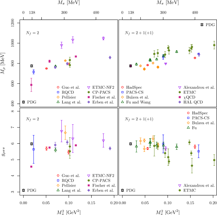
Figure 13: $M_{\rho}$ and $g_{\rho\pi\pi}$ as functions of $M_{\pi}^{2}$ for lattice results available in the literature with $N_{f}=2$, $N_{f}=2+1$ and $N_{f}=2+1+1$ dynamical quark flavors. For the references see the text.

The lightest vector-isovector unflavored meson, the so-called $\rho$-resonance, has been discussed throughout the current manuscript using different approaches. Due to its relatively small width and position far from the relevant inelastic thresholds it appears clearly as a prototypical resonance signal in, e.g., the phase-shifts of $\pi\pi$ scattering. Since the $\rho$ also represents the second lightest resonance in QCD, it became a benchmark state for lattice QCD calculations with the Lüscher method with first pioneering (pre-Lüscher) studies available in Refs. [339, 340].

Compared to other states, there are many publications available focusing on the $\rho$-resonance. Thus, we will concentrate in the following on results obtained with at least $N_{f}=2$ dynamical quark flavors and leave out quenched results. We will also not comment further on more approximate methods like the one presented in Refs. [117, 341]. Thus, we summarize the activity of studying the $\rho$-resonance on the lattice with the methodology discussed in Sec. 3. In order to avoid repetitions we refer for complimentary discussions to related reviews [342, 343, 344].

A variety of lattice QCD calculations of the $\rho$-resonance with $N_{f}=2$, $N_{f}=2+1$, and $N_{f}=2+1+1$ dynamical quark flavors exists. As discussed before, the corresponding phase-shift is estimated at different values of the pion mass, sometimes including ensembles with physical or almost physical value of the pion mass. Let us first focus on the results for mass and width (or coupling) of the $\rho$ obtained at the different (not necessarily physical) pion mass values and compare. Often, a Breit-Wigner fit to the phase-shift data is used to determine the resonance parameters, which for the $\rho$ does usually not differ significantly from better parametrizations like the IAM.

The bare lattice results for $M_{\rho}$ and the coupling $g_{\rho\pi\pi}$, related to $\Gamma_{\rho}$ via

$$\Gamma_{\rho}=\frac{2}{3}\frac{g_{\rho\pi\pi}^{2}}{4\pi}\frac{q_{\pi}^{3}}{M_{\rho}^{2}}\,,\qquad q_{\pi}=\sqrt{\frac{M_{\rho}^{2}}{4}-M_{\pi}^{2}}\,,$$ (5.1)

are plotted in Fig. 13 as functions of $M_{\pi}^{2}$. From the four panels, the two in the upper row depict $M_{\rho}$ and in the lower one $g_{\rho\pi\pi}$, while the two in the left column are for $N_{f}=2$ and in the right one for $N_{f}=2+1(+1)$. In fig. 13 we include $N_{f}=2$ results from Guo et al. [40], CP-PACS [345], RQCD [346], Lang et al. [347], ETMC-NF2 [111], Fischer et al. [348], Pelissier [349], and Erben et al. [350]. For $N_{f}=2+1$ we include PACS-CS [351], HadSpec [142], Bulava et al. [352], Fu and Wang [353], $\chi$QCD [354], Alexandrou et al. [355], Andersen et al. [356], HAL QCD [357] and for $N_{f}=2+1+1$ ETMC [358].

Let us mention that $\chi$QCD [354] has for the first time determined also $f_{\rho}$ using a partially quenched, mixed action approach with overlap valence fermions on a staggered sea. As a value they find $f_{\rho^{-}}=208.5(5.5)(0.9)\ \mathrm{MeV}$ in good agreement with the experimental value. While their value for $M_{\rho}$ is spot on and, thus, hiding behind the PDG value in fig. 13, they do not determine the width or the coupling. The coupling determined by HAL QCD in Ref. [357] has a value around $g_{\rho\pi\pi}\approx 12$ and is, therefore, not visible in Fig. 13.

In general the picture emerging from the different panels in fig. 13 is overall consistent, in particular for $N_{f}=2+1(+1)$ results. Exact agreement of all these results is not to be expected, because they are not extrapolated to the continuum limit and also different scale setting procedures are used. However, one can certainly conclude that the coupling has little pion mass dependence towards the chiral limit. The notable exception is the value for the coupling determined by HAL QCD, which is double the experimental value.

From fig. 13 it can be observed that the $N_{f}=2+1(+1)$ results appear to be more consistent. There is, in our opinion, no reason of principle for this. We rather assume that most of the $N_{f}=2+1(+1)$ results are more recent and have, thus, less uncontrolled uncertainties.

Let us next turn to extrapolations of the lattice results presented above to the physical pion mass value (assuming that the strange and charm quarks have been tuned to their physical values, if present.) The extrapolations have been performed either by the lattice practitioners themselves, or by other groups. The latter is the case for Niehus et al. [359], where lattice data from Ref. [352] and Ref. [142] is being analysed using different methods (see below) to extrapolate to the physical point. Similarly, Mai et al. [43] use data from Ref. [40]. In the works of $\chi$QCD [354] and RQCD [346] the $\rho$-resonance parameters have been even estimated directly with physical (or nearly physical) value of the pion mass, making an extrapolation unnecessary.

Reference	$N_{f}$	Pion mass	Chiral	Cont.	$M_{\rho}$ [MeV]	$\Gamma_{\rho}$[MeV]
		range [MeV]	extr.	extr.
ETMC-NF2-a [111]	2	$290-480$	VMEFT	x	$821(24)$	$171(31)$
ETMC-NF2-b [111]	2	$290-480$	mVMEFT	x	$850(35)$	$166(49)$
RQCD [346]	2	$150$	–	x	$716(30)$	$113(35)$
Fischer et al. [348]	2	$132-340$	IAM NLO	x	$786(20)$	$180(6)$
Guo et al. [40]	2	$226-315$	UCHPT	x	$720(15)$	$120(1)$
Mai et al. [43]	2	$226-315$	IAM NLO	x	$724(4)$	$133(2)$
$\chi$QCD [354]	2+1	139.2(4)	–	x	$776(6)$	-
Fu and Wang [353]	2+1	176-346	VMEFT	x	$780(16)$	$145(17)$
Niehus-a [359]	2+1	$200-284$	IAM NLO	($\checkmark$)	$761(25)$	$151(7)$
Niehus-b [359]	2+1	$200-284$	IAM NNLO	($\checkmark$)	$750(12)$	$129(12)$
Niehus-c [359]	2+1	$200-284$	IAM NLO	($\checkmark$)	$752(24)$	$145(5)$
Niehus-d [359]	2+1	$200-284$	IAM NNLO	($\checkmark$)	$738(7)$	$129(2)$
ETMC [358]	2+1+1	230-500	VMEFT	$\checkmark$	$769(19)$	$129(7)$
PDG [18]					$775.26(23)$	$147.4(8)$

Table 4: Overview over results on the $\rho$-resonance at the physical pion mass or extrapolated to the physical point based on lattice QCD. In some cases, when calculations at nearly physical pion mass were performed, chiral extrapolations were not performed (”–”). Where several errors are quoted in the original references, we combine them in quadrature. The last row shows the PDG value [18].

All the corresponding results are compiled in Tab. 4, where we quote $M_{\rho}$ and $\Gamma_{\rho}$ as determined in the corresponding references at the physical point. We also indicate the pion mass range used in the extrapolation and whether or not chiral and continuum extrapolations have been performed. The comparison is visualized in fig. 14.

For the chiral extrapolation different methods are being used:

• ”–”: the result from an ensemble directly at or close to the physical point is quoted and, thus, no extrapolation is performed.

• VMEFT: in Ref. [183] low-energy effective theory of vector mesons is studied using complex mass renormalization, see Sect. 4.2. The squared pion mass dependence of the complex squared pole $Z=(M_{\rho}+\mathrm{i}\Gamma_{\rho}/2)^{2}$ is determined, which allows one to extrapolate $M_{\rho}$ and $\Gamma_{\rho}$ together once these two observables have been determined for different pion mass values.

• mVMEFT: like EFT above, but modified according to Ref. [111] where instead of using $M_{\pi}^{2}$ as proxy for the average up/down light quark mass, the NLO chiral perturbation theory expression is used.

• UCHPT: unitarized chiral perturbation theory [266], see section 4.5.

• IAM: inverse amplitude method [163, 45, 280, 280], see section 4.5.

For the VMEFT and mVMEFT, mass and width need to be extracted for each ensemble before the chiral extrapolation is attempted. Here, typically a Breit-Wigner parametrization is adopted. For UCHPT and IAM one typically fits the phase-shifts or the lattice energy levels directly. We remind the reader that both UCHPT and IAM are representatives of a larger class of unitary approaches, see Sec. 4.5. The main qualitative difference lies in the matching to the strictly perturbative chiral expansion [137, 138]. Assuming a Breit-Wigner form certainly represents an approximation, which is, however, relatively well fulfilled for the $\rho$-resonance and also used for the analysis of experimental data.

Several comments are in order: currently, only in Ref. [358] a continuum extrapolation has been attempted in the sense that $a^{2}$ effects have been included in the fit, even if the corresponding fit parameters were found to be insignificant. Also in Ref. [352] several lattice spacing values have been studied. However, neither a continuum nor a chiral extrapolation has been performed. The same data is analysed in Ref. [359] using the IAM at NLO or NNLO. In the latter publication also the data at two different lattice spacing values from Refs. [360, 142] is analysed using the same method. In both cases, to our understanding, lattice artefacts have not been explicitly included in the fits, though such terms appear to be not required for describing the data. Moreover, in most of the analyses P-wave dominance was assumed with the notable exception of Ref. [360]. In the latter reference it was found, however, that this assumption is well justified.

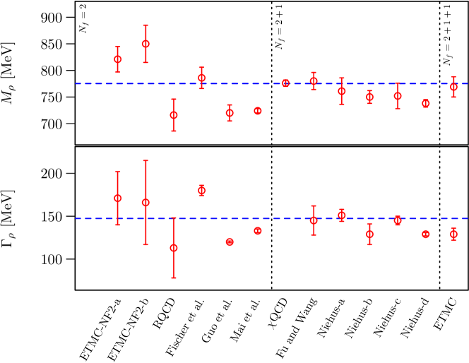
Figure 14: We compare the various literature values for $M_{\rho}$ (upper panel) and $\Gamma_{\rho}$ (lower panel) at the physical pion masses compiled in table 4 with the corresponding PDG values (blue, dashed line).

Comparing the extrapolated lattice results in Fig. 14 with the phenomenological information on the resonance parameters one observes that again for the $N_{f}=2$ results differences to the PDG values appear larger than for $N_{f}=2+1(+1)$, see also the discussion above. Since the differences are positive and negative alike, we do not think that one sees the difference between $N_{f}=2$ QCD and nature here. We would rather conclude that these differences can be attributed to lattice artefacts or other systematic differences between the investigations. Of course, in a $N_{f}=2$ flavor world the $\rho$-resonance might have different properties as compared to nature, but a fully controlled continuum and chiral extrapolations would be required to see such a difference. More detailed discussions can be found in Refs. [361, 362, 40, 363].

For $N_{f}=2+1$ and $N_{f}=2+1+1$, the agreement with the PDG value appears to be reasonable, though in some cases the deviations represent a few $\sigma$. Notably, the results from Ref. [359] using IAM to NNLO deviate further from the PDG value than the results based on IAM to NLO. The reason is likely too sparse data to constrain all parameters.

In general, we believe that lattice QCD results of the $\rho$-resonance at several lattice spacing values and several, close to physical pion mass values will be required to resolve the remaining discrepancies. Unfortunately, in the only reference so far with three lattice spacing values [358] the low pion mass region is not explored sufficiently well.

5.2 The $K^{*}(892)$-resonance

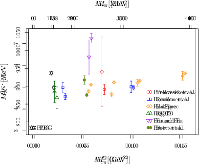
Figure 15: $M_{K^{*}}$ and $g_{K^{*}-K\pi}$ as functions of $M_{\pi}^{2}$ for lattice results available in the literature with $N_{f}=2$, $N_{f}=2+1$ and $N_{f}=2+1+1$ dynamical quark flavors. We show results by Prelovsek et al. [364], Rendon et al. [365], HadSpec [366], RQCD [346], Fu and Fu [367] and Brett et al. [368].

The $J^{P}=1^{-}$ $K^{*}$ resonance is the analogue of the $\rho$-resonance in the $K\pi$ channel with isospin $I=1/2$ decaying in a P-wave. Experimentally, a resonance mass of $M_{K^{*}}=892\ \mathrm{MeV}$ and a coupling $g_{K^{*}-K\pi}=5.73(6)$ is quoted [18].

The lattice status is certainly not yet comparable to the $\rho$-resonance: there are fewer results available and fewer systematic effects have been investigated and controlled. The first lattice computation has been performed using the Michael and McNeile method in Ref. [117], however, the validity of the method is more questionable for the $K^{*}$ than for the $\rho$.

In Ref. [364] (see also Ref. [369]) Prelovsek et al. then used the Lüscher method on a single $N_{f}=2$ flavor lattice QCD ensemble. An additional strange quark was added only in the valence sector. The pion mass of the ensemble is $M_{\pi}=266(4)\ \mathrm{MeV}$ and the strange quark mass was fixed using $M_{\phi}$. The authors find $M_{K^{*}}=891(14)$ and $g_{K^{*}-K\pi}=5.7(1.6)$ including only the P-wave, in surprisingly good agreement to experiment. In the same reference they also estimate the $K^{*}(1410)$ resonance mass including P- and D-wave mixing.

Rendon et al. study S- and P-wave scattering in the $I=1/2$ channel in Ref. [365] with two ensembles corresponding to pion mass values of $317$ and $176$ MeV. For the $K^{*}$ in the P-wave they find $M_{K^{*}}=895(6)\ \mathrm{MeV}$ and $M_{K^{*}}=871(8)\ \mathrm{MeV}$ for the heavier and the lighter pion mass value, respectively. For the coupling they quote $g_{K^{*}-K\pi}=5.02(26)$ and $g_{K^{*}-K\pi}=4.99(22)$. They use $N_{f}=2+1$ flavor CLS ensembles at two different values of the pion mass, $317$ and $175\ \mathrm{MeV}$, the lighter pion mass ensemble corresponding to the finer lattice spacing of $a=0.088\ \mathrm{fm}$ and the heavier one to $a=0114\ \mathrm{fm}$.

The Hadron Spectrum collaboration study the $K^{*}$ for several pion mass values in Ref. [366], after an initial study in Ref. [370]. The pion mass values range from $239$ to $391$ MeV and $I=1/2$ and $I=3/2$ are being investigated.

RQCD in Ref. [346] determine the $K^{*}$ on one $N_{f}=2$ ensemble with $M_{\pi}=150\ \mathrm{MeV}$. They carefully investigate systematics and arrive at $M_{K^{*}}=868(30)\ \mathrm{MeV}$ and $g_{K^{*}-K\pi}=4.79(49)$.

Brett et al. [368] work on a single ensemble with $230\ \mathrm{MeV}$ pion mass and $N_{f}=2+1$ dynamical quark flavors. Their result is $M_{K^{*}}/M_{\pi}=3.808(18)$ and $g_{K^{*}-K\pi}=5.33(20)$.

Fu and Fu [367] work with $N_{f}=2+1$ flavor MILC ensembles with the staggered quark discretization. The ensemble they use has a rather coarse lattice spacing of $a=0.15\ \mathrm{fm}$. They quote $M_{K^{*}}=1034(13)\ \mathrm{MeV}$ and $g_{K^{*}-K\pi}=6.38(78)$.

In Fig. 15 we summarize the current lattice status for the $K^{*}$: we show $M_{K^{*}}$ in the left and $g_{K^{*}-K\pi}$ in right panel, both as a function of $M_{\pi}^{2}$ comparing the results available in the literature. Since no continuum limits have been taken, the agreement is reasonable, maybe apart from the result from Fu and Fu in Ref. [367]. A possible explanation for the discrepancy they find might be the large lattice spacing of $0.15\ \mathrm{fm}$ or the staggered fermion formulation used in Ref. [367].

5.3 The $\Delta(1232)$-resonance

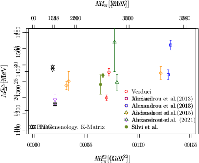
Figure 16: $M_{\Delta}$ and $g_{\Delta-N\pi}$ as functions of $M_{\pi}^{2}$ for lattice results available in the literature with $N_{f}=2$, $N_{f}=2+1$ and $N_{f}=2+1+1$ dynamical quark flavors. Results from Verduci [371], Alexandrou et al. [118, 372], Andersen et al. [373], Alexandrou et al. [374] and Silvi et al. [375] are shown.

The $\Delta(1232)$-resonance is decaying predominantly into nucleon-pion, it is well isolated and it represents the lowest lying spin-$3/2$ baryon resonance. For the $\Delta$(1232)-resonance the amount of lattice results is much sparser than for the $\rho$(770) and even the $K^{\ast}(892)$ discussed above. The main reason is that the signal-to-noise ratio in the relevant correlation functions is worse, since one is dealing with a heavier baryonic state. An additional complication comes from the fact that the inelastic threshold is relatively close by at $N\pi\pi$. This means on the one hand that the calculation needs to be done at close to physical pion mass and on the other that there are typically only very few energy levels available in the range between $N\pi$ and $N\pi\pi$. We remark here that the $N\pi\pi$ channel is subdominant and for this reason sometimes the elastic Lüscher formalism is applied also above the $N\pi\pi$ threshold.

Due to these limitations we include for the $\Delta(1232)$ all available lattice results in the comparison, where the $\Delta$ is treated as a resonance. After preliminary results for the $P_{33}$ phase-shift in pion-nucleon scattering have been shown in Ref. [376], results for mass and width have been reported in Verduci’s PhD thesis [371], where Lüscher’s formalism with $N_{f}=2$ Wilson-clover improved dynamical quarks was applied. The single ensemble had a pion mass value of $266\ \mathrm{MeV}$. The $\Delta$ mass and width are determined from a Breit-Wigner fit. In the two references by Alexandrou et al. [118, 372] the approach developed by Michael and McNeile was used instead of the Lüscher formalism. These calculations are based on domain wall valence fermions on a staggered sea with two pion mass values, $180$ and $260$ MeV. Andersen et al. [373] use one $N_{f}=2+1$ flavor CLS ensemble with $M_{\pi}=280\ \mathrm{MeV}$. The authors apply the Lüscher formalism and a Breit-Wigner fit to determine mass and width. Silvi et al. [375], again using $N_{f}=2+1$ dynamical quark flavors this time with a $255\ \mathrm{MeV}$ pion mass value, apply the Lüscher method to explore for the first time both a fit to the phase-shift data with a Breit-Wigner form and a determination of the pole in the scattering amplitude. The difference they find between these two methods is negligible within errors. Finally, in the proceeding contribution by Alexandrou et al. [374] $N_{f}=2+1+1$ dynamical flavor simulations are used for the first time with physical value of the pion mass. The fit to determine the mass and width relies on a Breit-Wigner form, but there is no value for the width quoted yet.

All these calculations are based on single lattice spacing simulations and single pion mass values each. Therefore, the meaningfulness of these calculations is limited. But we can learn that the lattice calculation of the $\Delta(1232)$ is feasible and we can expect more results in the near future. Moreover, by combining all available results, one sees a more or less consistent picture emerging: in fig. 16 we show in the left panel $M_{\Delta}$ and in the right panel $g_{\Delta-N\pi}$ as functions of $M_{\pi}^{2}$. The PDG value for the mass is included in the left figure, while in the right we take the average of the two values from Refs. [216, 377].

The coupling $g_{\Delta-N\pi}$ is defined here as in Ref. [216] via the width

$$\Gamma_{\Delta}=\frac{(g_{\Delta-N\pi})^{2}}{48\pi m_{N}^{2}}\frac{E_{N}+m_{N}}{E_{N}+E_{\pi}}p_{\Delta}^{3}$$ (5.2)

in order to be able to compare all the results. $E_{N}$ and $E_{\pi}$ are the energies of the nucleon and pion, respectively, with total momentum $p_{\Delta}$. Note that first steps towards studying the $\Delta$ resonance by HAL QCD can be found in Ref. [378].

The status of the $\Delta(1232)$ from lattice QCD is certainly not yet final. But the existing, though still more exploratory investigation indicate that this baryon resonance can be studied with good precision using lattice QCD. Like for the $\rho$-resonance, it will be interesting to see the continuum extrapolation of the data, but even more so the inclusion of $N\pi\pi$ in the investigations. It is likely that eventually the continuum limit needs to be taken at the physical point, since the applicability of CHPT for this state is at least questionable.

Let us also remark that it will be also very interesting to estimate the scattering length in the $I=1/2$ and $I=3/2$ channels as precisely as possible, since these scattering length can be compared to very precise experimental measurements. These scattering lengths are also important in the analysis of the pion-nucleon $\sigma$-term [379].

5.4 The $f_{0}(500)$-resonance

The scalar isoscalar unflavored mesonic resonance $f_{0}(500)$ (also referred to as $\sigma$-resonance) is the lightest excited state in the spectrum of hadrons. At the same time it is one of the most controversial as its appearance in the line-shapes of, e.g., $\pi\pi$ scattering is hard to distinguish from the unstructured background, see the extensive review [44]. Ultimately, many precise analyses led to the currently accepted ranges for mass and width [18].

Access to this ($I=\ell=0$) channel directly from quark-gluon dynamics using the above described methods of lattice QCD was hindered for a long time by the presence of disconnected diagrams, despite early pioneering works [380, 381, 382, 383]. The first full fledged calculation was finally performed by the Hadron Spectrum Collaboration [342], extracting also phase-shifts using the Lüscher framework. These results have then been analyzed and extrapolated to the physical point using the mIAM in Ref. [283]. Only a little later, a two-flavor lattice QCD study by the ETMC [384] was performed, allowing to extract and extrapolate $I=0$ $\pi\pi$ S-wave scattering length to the physical point. Note that recently a study in chiral perturbation theory has been performed in Ref. [385], results of which require to reassess the uncertainties quoted in Ref. [384]: the chiral perturbation theory result suggests that these are of the order of the result itself.

In Ref. [386] the scattering lengths were determined in the three-flavor formulation. The second calculation covering a larger energy region was performed by the GWQCD group in the two-flavor setup [41] extrapolating the obtained resonance parameters to the physical point using a chiral unitary approach.
Subsequently, the obtained energy eigenvalues were reanalyzed in a cross-channel ($I=0,1,2$) study [43], including chiral extrapolations using the mIAM approach [163, 45, 280, 280], see section 4.5, leading to tighter constraints on the resonance parameter values at the physical point.

In Ref. [387] coupled channel $\pi\pi$, $K\bar{K}$ and $\eta\eta$ scattering with isospin $I=0$ was studied for the first time. The authors work with one ensemble with a pion mass value of $391\ \mathrm{MeV}$ with $N_{f}=2+1$ dynamical quark flavors. The pion mass value of almost $400\ \mathrm{MeV}$ has implications for the thresholds. But in this setting they find a bound-state $f_{0}(500)$ pole on the physical Riemann sheet ${[+++]}$ at $745(5)\ \mathrm{MeV}$ mass and an $f_{0}$ resonance on the unphysical ${[-++]}$ Riemann sheet at $1166(45)-\mathrm{i}181(68)/2\ \mathrm{MeV}$. The $f_{0}(500)$, of course, becomes unstable once the pion mass is reduced towards the physical point. The $f_{0}$ resonance is connected by the authors to the $f_{0}(980)$ resonance, and they claim that it is dominated by a $K\bar{K}$ molecular state, because there is no pole on ${[--+]}$ Riemann sheet.

Reference	$N_{f}$	Pion mass	Chiral	$\sqrt{s_{\sigma}}$ [MeV]
		range [MeV]	extr.
GWQCD [41]	2	227-315	UCHPT	$440(52)-\mathrm{i}240(32)$
Mai et al. [43]	2	227-315	mIAM	$443(3)\phantom{0}-\mathrm{i}221(6)$
HadSpec [342] Döring et al. [283]	2+1	236-391	mIAM	$449(17)-\mathrm{i}169(24)$
PDG [18]				$450(50)-\mathrm{i}275(75)$

Table 5: The $\sigma$-resonance pole position $\sqrt{s_{\sigma}}$ at the physical pion mass value determined based on lattice QCD data. The last row shows the corresponding PDG value [18]. For none of these results the continuum limit has been studied.

The currently available lattice QCD results for the $f_{0}(500)$ or $\sigma$-resonance pole position $\sqrt{s_{\sigma}}$ at the physical point are compiled in table 5, where we also quote the PDG value. The agreement is reasonable, keeping in mind that most of the systematic effects are still not controlled in the corresponding lattice simulations.

6 Results: Coupled channels/thresholds

The vast majority of resonant states appear in settings allowing (energetically) for multiple decay channels. Such cases are harder to access both in performing numerical lattice QCD calculations as well as in view of the analysis of the results, extracting for example universal parameters of resonances from poles on the second Riemann sheet. In the following we review the current status on such states accessed from Lattice QCD. For the $D_{0}^{\ast}(2300)$ we also discuss recent extractions of the pole positions from recent LHCb data.

6.1 Light mesons

The mesonic scalar states $a_{0}(980)$, $f_{0}(980)$, $f_{0}(500)$ and $\kappa(800)$ were studied in Ref. [388] using quenched simulations for pion masses 344-576 MeV. In that, an effort was made to identify the tetraquark content of these states and searching for new states. Similar goals are followed in Ref. [381] for isospin $0$, $2$, $1/2$ and $3/2$ states. The question about the tetraquark content of the $a_{0}(980)$ and the $\kappa(800)$ was then further studied in an unquenched simulation [389], finding no evidence for such an interpretation. The $a_{0}(980)$ was extracted in a coupled-channel meson-meson scattering in lattice QCD in Ref. [390]. In the latter reference a global fit to lattice finite-volume energy levels from $\pi\eta$ scattering and to relevant experimental data on the $\pi\eta$ event distribution in $B$ decays together with the $\gamma\gamma\to\pi\eta$ cross section is performed. Both the leading and next-to-leading-order analyses lead to similar and successful descriptions of the finite-volume energy levels and the experimental data. However, these two different analyses yield different $\pi\eta$ scattering phase shifts for the physical masses of the pseudoscalar mesons. Both the $a_{0}(980)$ and the $a_{0}(1450)$ poles and their properties could be extracted at NLO.

The $f_{0}(980)$, discussed in section 5.4, was studied in Ref. [387] by investigating isoscalar $\pi\pi$, $K\bar{K}$ and $\eta\eta$ coupled channel scattering. The authors find a candidate state for the $f_{0}(980)$ and its properties suggest that it closest resembles a $K\bar{K}$ molecule. In this context it is worth emphasizing that the opening of the $K\bar{K}$ threshold induces a level crossing thus mocking up a resonance [391]. A possible resonance and a threshold can be distinguished by their different quark mass dependence.

Systems with non-vanishing strangeness quantum number ($\pi K$, $\eta K$) have been studied for a single pion mass ($\approx 400$ MeV) by the Hadron Spectrum Collaboration [370]. In that a generic parametrization of the scattering amplitude (Chew-Mandelstam) was utilized to obtain the complex pole position on the second Riemann sheet. Extracted poles were found to be comparable to the experimental values even for the broader scalar case. For the narrow tensor resonance $K^{*}(1430)$ also Breit-Wigner parameters have been extracted as $M_{R}=933(1)~{}{\rm MeV}$ and $g_{R}=5.93(26)$. Later the study was repeated for a range of pion masses ($200-400$ MeV) in Ref. [366] tracing out the chiral trajectory of the resonance pole.

Also very interesting, but also more complex are light mesons decaying to multihadron states, such as the $a_{1}(1260)$, which are hard to access both on the lattice and in the continuum. For the former, one key challenge lies in the construction of multihadron interpolating operators. In a pioneering study [392] composite operators such as $\rho\pi$, $\omega\pi$ etc. were used. Three particle operators were not considered motivated by the fact that for the considered setup ($L\approx 2~{}{\rm fm}$, $M_{\pi}=266~{}{\rm MeV}$) the three pion states are above the considered energy range. With these set of interpolating operators it was observed that the inclusion of composite operators in the GEVP (see section 3.4) is crucial for a stable extraction of energy levels. In this work also a finite-volume analysis was performed using the two-body Lüscher formalism and the Breit-Wigner parametrization of the scattering amplitudes, both rooting in the same approximation of stable vector mesons. The resonance masses were extracted as $M_{a_{1}}=1.435^{+53}_{-121}~{}{\rm GeV}$, $M_{b_{1}}=1.435^{+36}_{-90}~{}{\rm GeV}$ comparing roughly with the experimental values [18], $1.230(40)~{}{\rm GeV}$ and $1.2295(32)~{}{\rm GeV}$, respectively.

Later, a lattice calculation of coupled $\pi\omega$, $\pi\phi$ scattering was reported by the Hadron Spectrum Collaboration in Ref. [393]. While three-meson interpolators were included systematically, the finite-volume effects of the three-body channels were only included via meson-meson channels, motivated by the large pion mass $M_{\pi}=391~{}{\rm MeV}$ of the considered ensemble. A clear resonance signal for the $b_{1}$-resonance was observed with the $M_{R}\approx 1380~{}{\rm MeV}$.

Recently, the resonant three-pion channel for the quantum numbers of the $a_{1}$-resonance was calculated on the lattice by the GWQCD collaboration [38]. Here, for a pion mass value of 224 MeV the interpolator basis also included one-, two- and three-meson interpolators. Similarly to the pioneering study of Lang et al. [392], it was observed that three-body operators are, indeed, indispensable for a stable extraction of energy eigenvalues. The results of this calculation were used to determine volume-independent quantities by the means of the recently developed three-body quantization condition [85, 86]. Subsequently, these quantities were used to obtain a pole position on the second Riemann sheet, see left panel of Fig. 4. Couplings of the $a_{1}$-resonance could be extracted via the corresponding infinite-volume three-body formalism [39, 27]. Agreement of the mass of this state with the experimental value was observed, while the width was found to be significantly smaller than its experimental counterpart. This is certainly expected having a lattice setup with heavier than physical pion mass values.

6.2 The Roper-resonance $N(1440)$

The $N(1440)$ or Roper resonance [394] is the first excited nucleon state with $I(J^{P})=1/2(1/2^{+})$ quantum numbers. It appears in the baryon spectrum as a considerably lighter state than the parity partner of the nucleon $I(J^{P})=1/2(1/2^{-})$ $N(1535)$ which is at odds with quark model expectations [395, 396, 397] associating the Roper with the second radial excitation of the nucleon. This comprises one of the paramount examples of the baryon spectrum puzzles, see also the discussion in Sec. 4.4. Note that better agreement with phenomenology can be achieved by including Goldstone bosons as effective degrees of freedom to the constituent quark model [398]. Also more recent phenomenological analyses reveal an intricate analytic structure of the Roper [399, 37, 400] including strong coupling to the three-body channels distorting its shape from the usual Breit-Wigner form. Theoretical explanations include its dynamical generation without a $qqq$ core [401], or an interplay of genuine resonance poles and dynamical effects [402].

In modern LQCD calculations, the Roper channel is similarly obscure despite significant efforts made to reveal its structure, see for instance Refs. [403, 404, 405, 406, 407, 408]. Among the references from above, only in Ref. [406] evidence for a state compatible in mass with the $N(1440)$ was claimed, using a chiral fermion discretization and a Bayesian ansatz to estimate the energy levels. However, the calculation is partially quenched and utilizes mixed action (even though chiral valence on chiral sea) and, maybe most importantly, the Roper is to our understanding not treated as a resonance, e.g., with the Lüscher formalism.

More sophisticated LQCD studies [409, 410] followed later, consistently ruling out the exclusive $qqq$ interpretation of the Roper-resonance. Instead the sizable coupling to the five-quark operators (meson-baryon states) is noted in Ref. [410]. Even more interesting, is the missing level reported in Ref. [409, 143, 411] to the expectation from the elastic $\pi N$ scattering alone. While there are attempts based on Hamiltonian effective field theory (HEFT) [412] to interpret the measured finite-volume spectrum [409], an obvious solution to this seem to be the not included (most notably $\pi\pi N$) inelastic channels. Notably, this is also supported by phenomenology [18] attributing up to 50% of the decay branching ratio to such three-body channels in the final state, as discussed in Sec. 4.4.

In the context of $\pi N$ scattering we mention that there is also an exploratory study by Lang and Verduci [413] in the negative parity sector, which reports a significant change of the calculated finite-volume spectrum when extending the operator basis to incorporate the meson-baryon type operators. Finally, the situation may become even more entangled as discussed in Ref. [414]. There, based on a chiral unitary approach for the meson-baryon scattering [260, 415] a finite-volume spectrum for the $I(J^{P})=1/2(1/2^{-})$ channel was predicted using quark masses from lattice studies [416, 417]. It was found that mixing of relevant two-body thresholds ($\eta N,K\Lambda,K\Sigma$) can induce spectra looking similar to an avoided level crossing. Furthermore, poles can move on hidden Riemann sheets, thus, obscuring simple level counting arguments. Future analyses have to face such challenges in both parity sectors, in addition to the complexity of the three-body channels (see e.g. [29]) for $N^{*}(1440)$ channel.

6.3 Specific Open and Closed Charm Systems

There is significant focus on determining properties of charmonium resonances from Lattice QCD. One reason for this is that the charmonium spectrum was long believed to be well understood in terms of a heavy quark potential (the positronium of QCD) but with the appearance of quite a number of “exotic” states like the $X(3872)$ (nowadays called $\chi_{c1}(3872)$) challenged this simple picture and rekindled interest.

There is a list of lattice QCD studies of charmed meson states, which are mostly of exploratory nature. However, the studies represent important technical progress and allow one to draw first physical conclusions. There are several groups or collaborations which successively worked on different states based on a fixed lattice action and fixed ensembles.

The work of the group around Lang, Mohler and Prelovsek is largely based on two ensembles: one with $M_{\pi}=266\ \mathrm{MeV}$ and $N_{f}=2$ and a second one with $M_{\pi}=156\ \mathrm{MeV}$ and $N_{f}=2+1$ dynamical quark flavors. As a consequence, the charm quark is always treated partially quenched, which has a technical advantage: a charm and anti-charm cannot be created from the vacuum, which makes certain decays to (much) lighter states impossible. For the $N_{f}=2$ ensemble the strange is partially quenched as well.

The CLQCD collaboration on the other hand works with $N_{f}=2$ Wilson twisted mass ensembles generated by the European Twisted Mass Collaboration (ETMC) [418, 419] with a range of pion mass values from $300\ \mathrm{MeV}$ to $458\ \mathrm{MeV}$. They work with a relatively fine lattice spacing value of $0.067\ \mathrm{fm}$. Thus, while they can investigate the pion mass dependence to some extend, lattice artefacts are also not accessible, but are expected to be small. In that, it is notable that with Wilson twisted mass fermions at maximal twist, lattice artefacts linear in $am_{c}$ are absent and contributions start only at $(am_{c})^{2}$.

Similarly, two-meson systems involving $D$ mesons have been also studied by the Hadron Spectrum Collaboration. Their work is based on lattice QCD ensembles with $N_{f}=2+1$ dynamical quark flavors and anisotropy. The relevant ensembles for this review are one with pion mass value $391\ \mathrm{MeV}$ and a second one with $M_{\pi}=239\ \mathrm{MeV}$. Their usage of the distillation method [134, 135] allows them to include a large set of interpolating operators. The resulting number of energy levels and the precision thereof allows them to perform elaborate analyses including also coupled channels. The price for such resource intensive investigations is that typically those are only performed on one or two ensembles, which makes the understanding of systematics and, thus, the generalisation of the results harder. For a first investigation of the $D$-meson spectrum see Ref. [420], which, however, treats all states as stable states.

6.3.1 The $D_{0}^{*}(2300)$

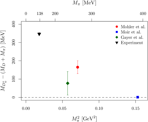
Figure 17: Comparison of $D_{0}^{\ast}(2300)$ energies from the different lattice calculations minus $M_{D}+M_{\pi}$ as a function of the squared pion mass value.

The $D_{0}^{*}(2300)$ (formerly known as $D_{0}^{\ast}(2400)$) is a state with $J^{P}=0^{+}$ and isospin $I=1/2$, seen to decay into $D\pi$. The width of the state is quoted to be around $220\ \mathrm{MeV}$ by the PDG [18].

In Ref. [421] Mohler and co-authors study $D$-meson pion scattering and $D$-meson resonances. It represents an exploratory study of the scalar $D_{0}^{*}(2300)$ and the axial $D_{1}(2430)$ resonances on the one aforementioned $N_{f}=2$ ensemble with a pion mass value of about $266\ \mathrm{MeV}$. Consequentially, the charm quarks are treated partially quenched. Since they do not work at physical pion mass value they quote mass differences with respect to the spin-average $(M_{D}+3M_{D^{\star}})/4$ for the $D_{0}^{*}(2300)$, for which they quote $351(21)\ \mathrm{MeV}$ in agreement with the experimental value. The coupling of the $D_{0}^{*}(2300)$ to $D\pi$ is found to be $g_{D_{0}^{*}D\pi}=2.55(21)\ \mathrm{GeV}$, only a few $\sigma$ away from the experimental value. In addition, the authors determine energy levels for a list of states in the $D$-meson spectrum. Given the fact that they are not able to extrapolate to the continuum limit nor to the physical pion mass value, the agreement to experiment is quite remarkable. Finally, they also determine the S-wave scattering lengths for the $D\pi$ and the $D^{*}\pi$ systems with $I=1/2$, finding $a_{0}=0.81(14)\ \mathrm{fm}$ and $a_{0}=0.81(17)\ \mathrm{fm}$, respectively. It should be noted that the spatial volume is only $16^{3}$.

In Ref. [303] a first coupled channel analysis of $D\pi$, $D\eta$ and $D_{s}\bar{K}$ scattering is presented by the Hadron Spectrum Collaboration based on the aforementioned ensemble with the largest pion mass ($N_{f}=2+1$, $M_{\pi}=391\ \mathrm{MeV}$. Scattering amplitudes are determined and analytically continued to complex energies. This results in finding a shallow bound state at $2276(1)\ \mathrm{MeV}$ below the $D\pi$ threshold in the $J^{P}=0^{+}$ channel, which could be the $D_{0}^{*}(2300)$. Another – this time deeply-bound state in the $1^{-}$ channel – is found at $2009(2)\ \mathrm{MeV}$, which could be related to the $D^{*}(2007)$. A resonance is found in the $J^{P}=2^{+}$ channel, which is narrow and has mass and width of $2527(3)\ \mathrm{MeV}$ and $8.2(7)\ \mathrm{MeV}$, respectively. While experimentally, this could correspond to the $D_{2}^{*}(2460)$, we remark that the $D^{*}\pi$ is not included in this investigation.

The data of Ref. [303] were reanalyzed in the framework of UCHPT [302] as discussed in Sect. 4.5.4. The NLO effective Lagrangian was utilized together with the LECs determined earlier in [323] to calculate the energy levels for $J^{P}=0^{+}$scattering in the strangeness-isospin $(S,I)=(0,1/2)$ in a finite volume [422, 423]. This not only led to an amazingly precise postdiction of the energy levels, but indeed the two pole structure of the $D_{0}^{*}(2300)$ was revealed with the following pole positions ($\sqrt{s}=M-\mathrm{i}\Gamma/2$):

$$\text{Pole~{}1:}~{}~{}(2264^{+8}_{-14}-\mathrm{i}0)~{}{\rm MeV}\,,~{}~{}~{}~{}~{}~{}~{}~{}~{} \text{Pole~{}2:}~{}~{}(2468^{+32}_{-25}-\mathrm{i}113^{+18}_{16})~{}{\rm MeV}~{},~{}~{} M_{\pi}=391~{}{\rm MeV}~{},$$

$$\text{Pole~{}1:}~{}~{}(2105^{+6}_{-8}-\mathrm{i}102^{+10}_{-12})~{}{\rm MeV}\,,~{}~{} \text{Pole~{}2:}~{}~{}(2451^{+36}_{-26}-\mathrm{i}134^{+7}_{8})~{}{\rm MeV}\,,~{}~{}~{} M_{\pi}=139~{}{\rm MeV}\,,$$ (6.1)

which solved the puzzle that the lowest charm-strange excitation was not heavier than the corresponding charm-nonstrange meson. This two-pole structure can be understood easily in the SU(3) limit. In this limit, all light and all heavy mesons take common values, see also Refs. [264, 319], and the heavy-light meson scattering amplitude decomposes into irreps as $\overline{\bf 3}\otimes{\bf 8}=\overline{\bf 15}\oplus{\bf 6}\oplus\overline{\bf 3}$ and the potential can be diagonalized accordingly. As it turns out, at leading order only the ${\bf 6}$ and $\overline{\bf 3}$ irreps are attractive, leading to two distinct poles. To make contact to the broken SU(3) world, linear extrapolations in the meson masses are used (as introduced in Ref. [36]), and the poles move into the complex plane as given in Eq. (6.3.1). In fact, the lower pole and the $D_{s0}^{\ast}(2317)$ discussed below are chiral partners in such a scenario. Using heavy-flavor symmetry, the same approach predicts a two-pole structures in the $(0,1/2)$ sector, located at $\sqrt{s}=5537^{+9}_{-11}-\mathrm{i}116^{+14}_{-15}~{}{\rm MeV}$ and $\sqrt{s}=5840^{+12}_{-13}-\mathrm{i}25^{+6}_{-5}~{}{\rm MeV}$. For $(S,I)=(1,0)$ the $D_{0}^{*}(2317)$ is found at $2315^{+18}_{-28}$ MeV as in [323] and the corresponding state in the $B$ meson sector is predicted at $5724^{+17}_{-24}$ MeV, i.e., it is bound by about 50 MeV. For an earlier study of these states, see [304]. Using heavy quark spin symmetry, one can make further predictions for axial $D_{1}$ and $B_{1}$ mesons. This double-pole structure is further consolidated by the analysis of data on $B\to D\phi\phi$ decays as discussed in Sect. 6.3.2.

Reference	$N_{f}$	$M_{\pi}\ [\mathrm{MeV}]$	$M_{D_{0}^{\ast}}-(M_{D}+M_{\pi})\ [\mathrm{MeV}]$
Mohler et al. [421]	2	266	165(33)
Moir et al. [303]	2+1	391	-1(1)
Gayer et al. [424]	2+1	239	77(64)
PDG [18]			347(7)

Table 6: The values extracted from the mentioned references for $M_{D_{0}^{\ast}(2300)}$ used for fig. 17.

In the $I=1/2$ channel, $D\pi$ scattering was investigated again in Ref. [424] by the Hadron Spectrum Collaboration with one ensemble at $M_{\pi}=239\ \mathrm{MeV}$. A $D_{0}^{*}$ resonance pole is found in the S-wave $D\pi$ system. Mass and width of $2196(64)\ \mathrm{MeV}$ and $425(224)\ \mathrm{MeV}$, respectively, are found by analytically continuing scattering amplitudes. This study complements the earlier study [303] at $M_{\pi}=391\ \mathrm{MeV}$ pion mass value. In contrast to the latter, the pole is now about $80\ \mathrm{MeV}$ below the $D\pi$ threshold, indicating a non-trivial pion mass dependence of this state. As discussed below, this result gives further credit to the lower pole in Eq. (6.3.1) representing the lowest charm scalar meson, see also Sect. 6.3.2.

The $D_{0}^{\ast}$ energies relative to the $D\pi$ threshold are plotted in Fig. 17 as a function of $M_{\pi}^{2}$ comparing the different available lattice estimates. Note that in Ref. [421] this energy difference is not quoted and we have determined it from the available results in that reference. The picture, which starts to emerge, seems to indicate that the $D_{0}^{\ast}$ is a virtual state above $M_{\pi}\approx 400\ \mathrm{MeV}$. Within the large uncertainties the available data lets one expect convergence towards the experimental value once the physical pion mass is used in lattice calculations.

6.3.2 The $D_{0}^{\ast}(2300)$ from Experimental Data

As discussed before, certain open charm mesons do not fit into the conventional quark model picture but rather are most probably hadronic molecules, which explains many of their odd features that are observed and also found on the lattice. This is further corroborated by the analysis of the precise data from LHCb on the various decay modes $B\to D\phi\phi$ [338, 306, 307, 308, 309], that give independent information on the thought after excited $D$ mesons in the S-wave amplitudes, that can be extracted from the so-called angular moments discussed in Sect. 4.5.4.

In this context, it is important to stress that the chiral symmetry of QCD requires energy-dependent pionic strong interactions at low energies. This constraint, however, is not fulfilled by the usual Breit-Wigner (BW) parameterization of pionic resonances, such as the open charm excitations discussed here, leading to masses larger than the real ones [336]. For an early work on this issue, see Ref. [425]. The argument goes as follows: Neglecting for simplicity the energy dependence of the decay width, the BW paramterization in the S-wave ($\ell=0$) of the $D\pi$ system reads:

$${\rm BW}_{0}(s)\propto\dfrac{1}{s-M_{0}^{2}+\mathrm{i}M_{0}\Gamma_{0}},$$ (6.2)

with $M_{0}$ and $\Gamma_{0}$ the BW mass and width of the resonance, in order. The peak position of this BW parameterization is given by

$$\dfrac{d}{ds}|{\rm BW}_{0}(s)|^{2}\propto-\dfrac{2(s-M_{0}^{2})}{\big{[}(s-M_{0}^{2})^{2}+M_{0}^{2}\Gamma^{2}_{0}\big{]}^{2}}=0~{}.$$ (6.3)

Thus, the BW mass for a resonance corresponds to the value of the peak position. The chiral symmetry constraints can be most simply accounted for by modifying Eq. (6.2) with an energy-dependent prefactor:

$${\rm BW}_{0}^{\prime}(s)\propto\dfrac{E_{\pi}}{s-M_{0}^{2}+\mathrm{i}M_{0}\Gamma_{0}}~{},~{}~{}E_{\pi}=\dfrac{s+M_{\pi}^{2}-M_{D}^{2}}{2\sqrt{s}}\,,$$ (6.4)

which is nothing but the energy of the produced soft pion in the rest frame of the $D\pi$ system. The peak position $s_{\text{peak}}$ is obtained from

$$\dfrac{d}{ds}|{\rm BW}_{0}^{\prime}(s)|^{2}\Big{\arrowvert}_{s=s_{\text{peak}}}=0\,,$$ (6.5)

which clearly yields a shift of $s_{\text{peak}}$ from $M_{0}^{2}$. This shift is expected to be small compared with $M_{0}$ as long as the width is small, $\Gamma_{0}\ll M_{0}$. Setting $s_{\text{peak}}=(M_{0}+\Delta)^{2}$ and retaining only the linear term in $\Delta$ leads to

$$\Delta\simeq\dfrac{\Gamma_{0}^{2}(M_{0}^{2}-M_{\pi}^{2}+M_{D}^{2})}{2M_{0}\big{[}2(M_{0}^{2}+M_{\pi}^{2}-M_{D}^{2})-\Gamma_{0}^{2}\big{]}}=\dfrac{\Gamma^{2}_{0}E_{D}}{4M_{0}E_{\pi}-\Gamma_{0}^{2}}\,,$$ (6.6)

where $E_{D}$ is the energy of the produced $D$ in the rest frame of the $D\pi$ system with total energy $M_{0}$. Thus, for the case $4M_{0}E_{\pi}>\Gamma_{0}^{2}$, the shift $\Delta$ is positive and the mass of the resonance is lower than the peak position. Note that the modification in Eq. (6.4) can only be applied in a small energy region before the coupled-channel effect becomes important, and, thus, is neither practical nor systematic. However, this little exercise clearly shows the deficiencies of the BW parameterization for pionic resonances that are severely constrained by chiral symmetry.

Using the framework outlined in Sect. 4.5.4, one can now fit the LHCb data for the reactions $B^{-}\to D^{+}\pi^{-}\pi^{-}$, $B^{-}\to D^{+}\pi^{-}K^{-}$, $B_{s}^{0}\to\bar{D}^{0}K^{-}\pi^{+}$, $B^{0}\to\bar{D}^{0}\pi^{-}\pi^{+}$ and $B^{0}\to\bar{D}^{0}\pi^{-}K^{+}$. In fact, note that only three sets of the weak production vertices in Table 3 are independent. Thus instead of fitting the four decay amplitudes to the experimental angular moments simultaneously, we fix the LECs in the amplitudes in Eqs. (4.97-4.100) by fitting to three of them, i.e., $B^{-}\to D^{+}\pi^{-}K^{-}$, $B_{s}^{0}\to\bar{D}^{0}K^{-}\pi^{+}$ and $B^{0}\to\bar{D}^{0}\pi^{-}\pi^{+}$, and then describe the angular moments for $B^{0}\to\bar{D}^{0}\pi^{-}K^{+}$ with the determined LECs. The data for the angular moments defined in Eqs. (4.5.4) and (4.104) are fitted up to $M_{D\pi}=2.54$ GeV as in Ref. [310] for the decays $B^{-}\to D^{+}\pi^{-}K^{-}$ and $B^{0}\to\bar{D}^{0}\pi^{-}\pi^{+}$, and up to $M_{\bar{D}\bar{K}}=2.65$ GeV for $B_{s}^{0}\to\bar{D}^{0}K^{-}\pi^{+}$ as in Ref. [336]. The best fit has a reasonable quality with $\chi^{2}/\text{d.o.f.}=1.2$ and the comparison to the LHCb data is shown in Fig. 18. The bands in this figure reflect the one-sigma errors of the parameters in the scattering amplitudes determined in Ref. [323].

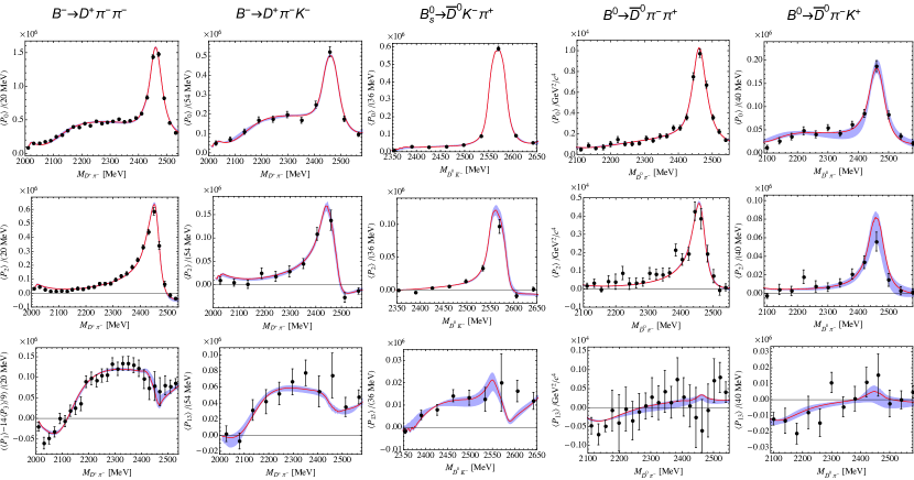
Figure 18: Fit to the LHCb data of the angular moments $\langle P_{0}\rangle$, $\langle P_{2}\rangle$ and $\langle P_{13}\rangle$ [338, 306, 307, 308, 309] for the various $B\to D\phi\phi$ channels. The largest error of $\langle P_{1}\rangle$ and $14\langle P_{3}\rangle/9$ in each bin is taken as the error of $\langle P_{13}\rangle$. The error bands correspond to the one-sigma uncertainties propagated from the input scattering amplitudes. All data sets are fit with two parameters (one combination of LECs and one subtraction constant) except for the fit to $B^{0}\to\bar{D}^{0}\pi^{-}K^{+}$, which only requires a subtraction constant as explained in the text.

We note that in particular the linear combination of two angular moments $\langle P_{13}\rangle=\langle P_{1}\rangle-{14}\langle P_{3}\rangle/9$ only depends on the S-P interference as long as one restricts oneself to partial waves with $\ell\leq 2$. Therefore, $\langle P_{13}\rangle$ is the quantity that one should focus on if one wants to better understand the scalar charmed mesons. The LHCb angular moment data for all these decays can be well described. The predicted $\langle P_{1}\rangle$ and $\langle P_{3}\rangle$ also agree with the measurements. Because the final-state interactions in these fits are taken from the unitarized chiral perturbation theory amplitudes already pinned down in Ref. [323], this analysis of the LHCb data implies that the poles contained in these amplitudes can be regarded as the low-lying scalar charmed meson spectrum. Furthermore, it follows that such a spectrum is consistent with the LHCb data. In particular, the poles of the scalar charm-nonstrange mesons, $\left(2105^{+6}_{-8}-\mathrm{i}\,102^{+10}_{-11}\right)$ MeV and $\left(2451^{+35}_{-26}-\mathrm{i}\,134^{+7}_{-8}\right)$ MeV [310], are different from the resonance parameters of the $D_{0}^{\ast}(2400)$ listed in Review of particle Physics (RPP) [426], which were extracted using a simple BW parameterization. The analysis in this work gives a further strong support to the two-$D_{0}^{*}$ scenario as advocated in Refs. [302, 310]. The two-pole scenario will be at least mentioned in the newest version of the RPP [18]. This point was further strengthened by the analysis in Ref. [427], the results based on unitarized CHPT were refined by using Khuri-Treiman equations, that respect three-body unitarity. The S-wave $D\pi$ phase-shift could be extracted and it was shown again that a BW parameterization is not capable of describing these data. Thus, the lightest charmed scalar meson is of similar nature than the famous $f_{0}(500)$ and $K_{0}^{\ast}(700)$, namely generated by meson-meson final-state interactions, which leads to masses at odds with quark model expectations.

6.3.3 The $D_{s0}^{*}(2317)$

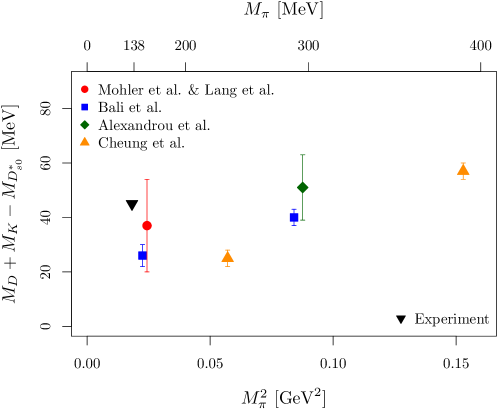
Figure 19: $M_{D}+M_{K}-M_{D_{s0}^{\ast}(2317)}$ as a function of $M_{\pi}^{2}$ comparing the available lattice determinations.

The $D_{s0}^{*}(2317)^{\pm}$ has isospin $I=0$ and appears to have quantum numbers $J^{P}=0^{+}$. It decays predominantly into $D_{s}^{+}\pi^{0}$ and has a width of only a few MeV. The PDG quotes a value of $M_{D_{s0}^{\ast}}=2317.8(5)\ \mathrm{MeV}$ and a width smaller than $4\ \mathrm{MeV}$ [18].

The first indirect lattice calculation of the $D_{s0}^{*}(2317)$ was performed in Ref. [323]. More precisely, the scattering lengths for the channels that are not affected by disconnected diagrams, namely $I=3/2$ $D\pi$, $D_{s}\pi$, $D_{s}K$, $I=0$ $D\bar{K}$ and $I=1$ $D\bar{K}$ (see Tab. 1), were calculated for pion masses in the range from 300 to 600 MeV. Using UCHPT at NLO, see Eq. (4.5.4), the LECs $h_{i}$ could be determined and predictions for the channels that were not explicitly calculated on the lattice could be made. The scattering length in the interesting channel $(S,I)=(1,0)$ was found to be $a(DK(I=0))=-0.84^{+0.17}_{-0.22}\,$fm and the pole position of a bound state comes out as $2315^{+18}_{-28}~{}{\rm MeV}$, which is very close to the PDG value of the mass of the $D_{s0}^{*}(2317)$. The molecular nature of this state is supported by the Weinberg argument, that relates the scattering length $a$ to the binding energy $\varepsilon$ and the wave function renormalization constant $Z$, with $(1-Z)$ being the probability of finding the molecular component in the physical state (note that $Z=0$ corresponds to a compact multi-quark state) [428, 429]. This relation reads

$$a=-2\left(\dfrac{1-Z}{2-Z}\right)\dfrac{1}{\sqrt{2\mu\varepsilon}}+{\cal O}(1/\beta)~{},$$ (6.7)

with $\mu$ the reduced mass and $1/\beta$ the range of forces. For a pure molecular state with $Z=0$, this equation gives $a=-1.05\,$fm, which coincides with the range given above. In fact, the trajectory of the pion mass dependence of such a molecular state is of quadratic shape [328], consistent with the lattice data of Ref. [430]. Finally, we note that the width of the $D_{s0}^{*}(2317)$ is very tiny, as it is entirely driven by isospin-breaking effects [431, 432, 318, 315].

Mohler et al. [433] carried out a similar exploratory calculation for $DK$ scattering focused on the $D_{s0}^{*}(2317)$. They find the $D_{s0}^{*}$ to be located $37(17)\ \mathrm{MeV}$ below the $DK$ threshold. The calculation is based on two the ensembles of Lang, Mohler and Prelovsek mentioned above, one with $N_{f}=2$ dynamical quark flavors and $M_{\pi}=266\ \mathrm{MeV}$ and a second one with $M_{\pi}=156\ \mathrm{MeV}$ and $N_{f}=2+1$ dynamical quark flavors. Of course, given the totally different systematics on these two ensembles a combination of the results is difficult. However, their finding is a negative value of the $DK$ S-wave scattering length, which leads the authors to the conclusion stated above.

In Ref. [434] a similar set of authors work with the exact same $N_{f}=2$ and $N_{f}=2+1$ flavor ensembles as discussed in the previous paragraph. Here, they focus on $D_{s}$ mesons by studying $DK$ and $D^{*}K$ scattering in the $J^{P}=0^{+},1^{+},2^{+}$ channels. In the $J^{P}=0^{+}$ channel they find a state $37(17)\ \mathrm{MeV}$ below the corresponding threshold, which they identify to be the $D_{s0}^{*}(2317)$, in agreement with Ref. [433]. In the $1^{+}$ channel the $D_{s1}(2460)$ is $44(10)\ \mathrm{MeV}$ below $D^{*}K$ threshold with a considerable four-quark component. In the same channel a narrow $D_{s1}(2536)$ state above threshold for the ensemble with lighter pion mass value. In the $J^{P}=2^{+}$ channel the $D_{s2}^{*}$ is found close to its experimentally expected energy. The authors find that it is important to include $DK$ and $D^{*}K$ interpolating operators in their analyses, which is not surprising. Torres and co-authors also investigate the $D_{s0}^{*}(2317)$ and the $D_{s1}^{*}(2460)$ in Ref. [435] reanalysing data from Refs. [433, 434] discussed above but also extending the database to all available energy levels. An existence of bound state for the $KD$ and $KD^{*}$ channels was confirmed, improving also the determination of the scattering length compared to the original determination.

Reference	$N_{f}$	$M_{\pi}\ [\mathrm{MeV}]$	$M_{D}+M_{K}-M_{D_{s0}^{\ast}}\ [\mathrm{MeV}]$
Mohler et al. [433]	2	156	37(17)
Bali et al. [430]	2	150	26(4)
Bali et al. [430]	2	290	40(3)
Alexandrou et al. [436]	2+1	296	51(12)
Cheung et al. [437]	2+1	239	25(3)
Cheung et al. [437]	2+1	391	57(3)
PDG [18]			44.7(5)

Table 7: Results for the $M_{D_{s0}^{\ast}(2317)}$ extracted from the various references used in fig. 19.

Another study of the $D_{s0}^{*}(2317)$ and the $D_{s1}(2460)$ can be found in Ref. [430]. Here, two pion masses of $290\ \mathrm{MeV}$ and $150\ \mathrm{MeV}$ are investigated with different volumes at one relatively fine value of the lattice spacing with $N_{f}=2$. Using spin-averaged quantities, reasonable agreement with experiment is found. Not averaged energies show significant deviations from experiment, which the authors argue is due to lattice artefacts. Their Lüscher analysis includes two-quark and four-quark operators in the $J^{P}=0^{+}$ and $1^{+}$ sectors. Of these, the four-quark interpolating operators have proven essential to be able to extract the exotic states of interest. The authors are actually able to perform an infinite-volume extrapolation thanks to the many volumes they have available. This extrapolation appears to work well, and it makes a significant difference for the final energy values. They find that the mass of the $D_{s0}^{\ast}$ lies $26(4)$ MeV and $40(3)$ MeV (for light and heavy pion mass ensembles, respectively) below the $DK$ threshold (the authors actually quote asymmetric errors, we use here the larger of the two). The pion mass dependence found here exactly agrees with the one based on unitarized chiral perturbation theory [328]. The work of Ref. [430] is also the first to our knowledge which computes the decay constants of these states and compares them to those of pseudoscalar and vector $D$-mesons.

The $D_{s0}^{*}(2317)$ is also being investigated in Ref. [436] with one $N_{f}=2+1$ flavor dynamical quark ensemble with $M_{\pi}=296\ \mathrm{MeV}$. The authors report it $51\ \mathrm{MeV}$ below the relevant $DK$ threshold. They find the largest coupling in their operator basis to quark-antiquark interpolating operators with only a small coupling to $DK$ scattering states. Tetraquark interpolators essentially contribute nothing to the analysis of the $D_{s0}^{*}(2317)$.

In Ref. [437] the authors of the Hadron Spectrum Collaboration present an investigation of the $D_{s0}(2317)$ with similar techniques in to Ref. [436]. The authors study the elastic scattering amplitudes for $DK$ and $D\bar{K}$ scattering with $I=0$ and $I=0,1$, respectively. In this calculation two ensembles are included, the first with $M_{\pi}=391\ \mathrm{MeV}$ and the second one with $M_{\pi}=239\ \mathrm{MeV}$. They find evidence for the bound $D_{s0}^{*}(2317)$ below $DK$ threshold in the $J^{P}=0^{+}$ channel.

For the $D_{s0}^{\ast}(2317)$ all the evidence points towards a $DK$ molecular like state. The currently available lattice results are more or less consistent. In fig. 19 we summarize the status by plotting $M_{D}+M_{K}-M_{D_{s0}^{\ast}}$, resembling a binding energy, as a function of $M_{\pi}^{2}$. Plotting this mass difference and neglecting the width of this state is justified, because the state is so narrow. The observed differences between the different determinations are likely to be explained with lattice artefacts, which are uncontrolled in all the available studies. Therefore, the necessary next step should be an investigation of lattice artefacts in this system.

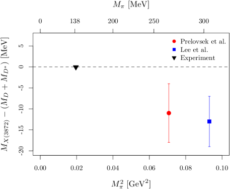
Figure 20: Comparison of the $X(3872)$ mass determined on the lattice by Prelovsek et al. in Ref. [438] and Lee et al. in Ref. [439].

6.3.4 The $X(3872)$

One of the first exotic states confirmed by several experiments in different decay channels was the $X(3872)$, a narrow charmonium like state, now denoted as $\chi_{c1}(3872)$. It was rather soon hypothesized to be a non quark-antiquark state. Its quantum numbers are $J^{PC}=1^{++}$ [440]. In order to understand its nature, lattice studies aim to use different interpolating operators to investigate the couplings of these operators to the state interpreted as the $X(3872)$. Recently, strategies to determine the $X(3872)$ from lattice QCD more precisely were formulated in Ref. [441]. Finite-volume corrections to the binding energy of the $X(3872)$ are discussed in Ref. [442].

The authors of Ref. [443] present a very first study of the $X(3872)$ exotic state. It is based on quenched lattice QCD and a chiral fermion discretization. Even though systematic uncertainties are not well controlled in this study and, in particular, no Lüscher like analysis has been performed, they find evidence for a state in the $1^{++}$ channel with about the correct energy. In another quenched study, CLQCD investigates the $\chi_{c2}$ in Ref. [444] and use their results to draw the conclusion that the $X(3872)$ has not $J^{PC}=2^{-+}$ as quantum numbers, which at the time of the publication was still not excluded.

In Ref. [445] Prelovsek and Leskovec study the $X(3872)$ state with $J^{PC}=1^{++}$ and zero isospin. This calculation is again exploratory in the sense that it is based on the same single $N_{f}=2$ ensemble with pion mass value of $266\ \mathrm{MeV}$ as used on Ref. [421] discussed above. They find a candidate for the $X(3872)$ just $11(7)\ \mathrm{MeV}$ below the $D\bar{D}^{*}$ threshold. Importantly, they find a large and negative value for the scattering length of the $D\bar{D}^{*}$ system of $-1.7(4)$, which allows them to identify the $X(3827)$ in their lattice data.

In the proceeding contributions [439] a candidate $X(3872)$ state is found just $13(6)\ \mathrm{MeV}$ below the $DD^{\ast}$ threshold with $I=0$. This study is based on a single ensemble with the HISQ staggered fermion discretization and $N_{f}=2+1+1$ dynamical quark flavors. This represents the only study of the $X(3872)$ including also a dynamical charm quark, though the character of this investigation is quite exploratory.

The $X(3872)$ was again studied in Ref. [446] by Padmanath and co-authors together with the $Y(4140)$. The authors work with the aforementioned $N_{f}=2$ ensemble at $M_{\pi}=266\ \mathrm{MeV}$. They find that it depends on the list of operators included in the analysis whether or not a $X(3872)$ candidate in the $I=0$ $J^{PC}=1^{++}$ channel can be found: $D\bar{D}^{*}$ and $c\bar{c}$ like interpolators appear to be a must. In the $I=1$ channel no neutral or charged $X(3872)$ candidate is found. Likewise, they find no evidence for a $Y(4140)$ state with $\bar{c}c\bar{s}s$ quark content.

The two available results from LQCD for $M_{X(3872)}-(M_{D}+D_{D^{\ast}})$ [438, 439] are compiled in fig. 20. Both have large uncertainty and were obtained for pion masses larger than $250\ \mathrm{MeV}$. Thus, it is probably not yet the time to compare with experiment on a quantitative level.

6.3.5 The $Z_{c}(3900)$

The $Z_{c}(3900)$ represents a closed charm state which might be of tetraquark nature with quark content $\bar{c}c\bar{d}u$. It has isospin $I^{G}=1^{+}$ and $J^{PC}=1^{+-}$. With a width of around $30\ \mathrm{MeV}$ it is relatively narrow and it is seen in different decay channels such as in $J/\psi\pi$, $\eta_{c}\pi\pi$, $D\bar{D}^{*}$ and $DD^{*}$. It was observed as a decay product of the exotic $Y(4260)$ state. We remark in passing that in Ref. [447] methodological developments for an improved lattice investigation of the $Z_{c}$ were presented.

Prelovsek and Leskovec search for a candidate $Z_{c}(3900)$ state in Ref. [448] in the $J^{PC}=1^{+-}$ with $I=1$, but do not find any evidence with $N_{f}=2$ dynamical quark flavors at $M_{\pi}=266\ \mathrm{MeV}$. This investigation was extended in Ref. [438]. Unfortunately, this study could also not reveal evidence for an extra $Z_{c}^{+}(3900)$ state in addition to all the expected two-meson states. The authors provide a detailed discussion as to why this is the case.

The CLQCD Collaboration studies the $Z_{c}(3900)$ in Ref. [449] in the scattering of $D\bar{D}^{*}$. They work with the three ensembles ($M_{\pi}=485,420,300$ MeV) with $N_{f}=2$ dynamical quarks discussed above. Noteworthy is their much smaller lattice spacing value than used in the studies by Prelovsek et al. [438] ($a=0.067\ \mathrm{fm}$ versus $a=0.125\ \mathrm{fm}$). They find a weak repulsive interaction between the $D$ and the $\bar{D}^{*}$ for all three pion mass values. Thus, their simulation results cannot support a bound state in the corresponding $J^{P}=1^{+}$ channel, where the $Z_{c}^{\pm}(3900)$ is expected.

We mention also two proceeding contributions investigating the $Z_{c}(3900)$ from lattice QCD. The first one [439] uses the staggered quark formulation, finding no candidate $Z_{c}^{+}(3900)$ state. The second [450] used $N_{f}=2$ Wilson twisted mass fermions, also not being able to corroborate the $Z_{c}$ interpretation as a $D\bar{D}^{\ast}$ bound state.

The HAL QCD collaboration studies the $Z_{c}(3900)$ in Ref. [451, 452] in a range of pion mass values from $400\ \mathrm{MeV}$ to $700\ \mathrm{MeV}$ taking into account coupled channels. Their data indicates that the $Z_{c}$ is most likely a threshold cusp.

It appears rather difficult to draw any conclusion from this list of lattice investigations. Mostly, there is no candidate $Z_{c}(3900)$ state found with the operators included in the respective analyses. Only HAL QCD finds indications for a threshold cusp.

Finite-volume spectra from of Prelovsek et al. [438] were further reanalysed in Ref. [337] using a unitarized amplitude, see Sec. 4.5. In that, they find that two scenarios are compatible with the lattice energy levels: a $D^{\ast}\bar{D}$ resonance or a virtual state. But they cannot distinguish between these two possibilities. They conclude that several volumes should be studied to obtain a better understanding of the $Z_{c}(3900)$.

6.4 Other Exotic States

In this subsection we present mainly exploratory studies of certain hadron resonances. Thus, we refrain from a discussion of the systematics or physics implications of the results.

6.4.1 States involving heavy-light mesons

The CLQCD collaboration investigated in Ref. [453] the exotic $Z_{c}(4025)$ state. S-wave scattering of $D^{*}\bar{D}^{*}$ was studied in the $J^{P}=1^{+}$ channel. Also here, CLQCD finds a weak repulsive interaction between the two mesons and, again, a bound state in this channel is not supported by their study. Like in the study of the $D\bar{D}^{*}$ this might be due to missing interpolators in the correlator matrix. But it could also be an effect of the unphysical pion mass values.

In Ref. [454] Lang and co-authors investigate vector and scalar charmonium resonances. In $D\bar{D}$ scattering they find the $\psi(3770)$ in the P-wave, as expected. However, in the scalar channel they find in S-wave $D\bar{D}$ scattering an additional state with mass slightly below $4\ \mathrm{GeV}$. This narrow resonance state was unobserved so far, while the ground state $\chi_{c0}(1P)$ is well understood. They investigate several scenarios for possible states in this channel and find that a scenario with the $\chi_{c0}(1P)$ and the additional narrow resonance mentioned above leads to a phase-shift consistent with experimental data. The authors work with the two ensembles again, one with $N_{f}=2$ and $M_{\pi}=266\ \mathrm{MeV}$ and the second one with $N_{f}=2+1$ and $M_{\pi}=156\ \mathrm{MeV}$.

In Ref. [455], however, CLQCD find a weakly attractive interaction in $\bar{D}_{1}D^{*}$ scattering based on the same ensembles and pion mass values. S- and P-wave channels have been studied finding attraction in both channels. Indications for bound states below threshold are reported, but further studies are needed to draw conclusions on the $Z_{c}(4430)$ exotic state.

A lattice QCD calculation of an $NJ/\psi$ and $N\eta_{c}$ system with quantum numbers overlapping with the quantum numbers of the LHCb discovered pentaquark states $P_{c}(4380)$ and $P_{c}(4450)$ was performed in Ref. [456]. The calculation was performed on two-flavor ensembles with $M_{\pi}=266~{}{\rm MeV}$, reaching for the first time energies of the mentioned pentaquark states. The calculation resulted in a very small (consistent with zero) attractive interaction, i.e., no significant energy shift from the non-interacting case was observed.

Positive parity $B_{s}$ mesons are investigated by Lang and co-authors in Ref. [457]. The investigation is based on a single $M_{\pi}=156\ \mathrm{MeV}$ ensemble with $N_{f}=2+1$ dynamical quark flavors. The bottom quark is added as a valence only quark with the Fermilab method, see Sect. 3.2.2. They identify the $B_{s1}(5830)$ and the $B_{s2}(5840)$ finding good agreement with experimental results. In addition they predict a $B_{s0}$ with mass $5750(25)\ \mathrm{MeV}$ in the $J^{P}=0^{+}$ channel. Based on the same single ensemble, Ref. [458] by Lang et al. represents the first $B_{s}\pi^{+}$ scattering study and its relation to the exotic $X(5568)$ from lattice QCD. As the main result, they cannot establish the $X(5568)$ from their lattice QCD simulation in the $J^{P}=0^{+}$ channel. Since the study is based on a single ensemble at a single lattice spacing only, this result does of course not exclude that such a state with these quantum numbers exists. Still its quantum numbers are also not yet finally determined experimentally and, thus, $J^{P}=0^{+}$ is only one possibility. Note that the $X(5568)$ poses severe challenges to QCD as discussed in Refs. [459, 460], for example such a mass is neither compatible with chiral symmetry nor with heavy quark symmetry.

In Ref. [461] the authors study the $J^{PC}=1^{--}$ and $J^{PC}=3^{--}$ channels in $\bar{D}D$ scattering. They use lattice ensembles with $280\ \mathrm{MeV}$ and two lattice volumes with $N_{f}=2+1$ quark flavors at a single lattice spacing value. In this reference the conventional $\psi(3770)$ and the $X(3842)$ are found at energies compatible with experiment. The investigation is extended to unconventional states in Ref. [462], where charmonium like resonances with $J^{PC}=0^{++}$ and $2^{++}$ in coupled $D\bar{D}$ and $D_{s}\bar{D}_{s}$ scattering are studied. In this study, Prelovsek et al. analytically continue the scattering matrix and determine pole singularities. They find a so far unobserved $D\bar{D}$ bound state just below threshold and a $D\bar{D}$ resonance, the latter of which they connect to the $\chi_{c0}(3860)$. Moreover, they find a narrow $J^{PC}=0^{++}$ resonance below $D_{s}\bar{D}_{s}$ threshold. They interpret it as possibly related to the $X(3915)$ or the $\chi_{c0}(3930)$ states. They also see a resonance they connect to the $\chi_{c2}(3930)$, because it is found in the D-wave.

Only very recently also the $I=0$ and $J^{P}=1^{+}$ channel was studied in $DD^{*}$ scattering on the ensemble from above with $280\ \mathrm{MeV}$ pion mass. Padmanath and Prelovsek [463] find evidence for a virtual bound state with just $10\ \mathrm{MeV}$ binding energy. This could be the doubly charmed tetraquark state recently discovered by LHCb [464, 465]. It has open charm quark content $cc\bar{u}\bar{d}$ and lies just order $1\ \mathrm{MeV}$ below the $D^{0}D^{\ast+}$ threshold.

Also, very recently axial-vector $D_{1}$ hadrons in $D^{\ast}\pi$ scattering were studied on a single $M_{\pi}=391\ \mathrm{MeV}$ ensemble for the first time in Ref. [466]. The dynamically coupled ${}^{3}S_{1}$ and ${}^{3}D_{1}$ channels in $D^{\ast}\pi$ scattering have been looked at, and the corresponding scattering amplitudes have been computed. The ${}^{3}S_{1}$ is dominated by the pole right below $D^{\ast}\pi$ threshold. The ${}^{3}D_{1}$ amplitude is dominated by a single, narrow resonance.

Doubly bottom tetraquarks have been investigated in Ref. [467] in an exploratory study without Lüscher analysis. Follow up investigations can be found in Refs. [468, 469]. The first Lüscher analysis for a $\bar{b}\bar{b}ud$ tetraquark with isospin $I=0$ and $J^{P}=1^{+}$ was performed in Ref. [470]. The work is based on domain wall fermion ensembles with $N_{f}=2+1$ dynamical quark flavors including an ensemble at the physical point. Their work controls most of the systematic uncertainties, the bottom quark is treated in the framework of lattice nonrelativistic QCD. They find significant evidence for the existence of a $\bar{b}\bar{b}ud$ tetraquark stable under strong and electromagnetic interactions. We remark that there is significant effort under way to study bottomonium, see for instance Ref. [471] by Ryan and Wilson, where only two quark operators have been used so far, or Ref. [472], where a formalism is proposed and derived based on static potentials. The latter is applied in Ref. [473] to study among others bottomonium in different partial waves with $I=0$.

In Ref. [474] a study of the $\bar{b}\bar{b}us$ us system with quantum numbers $J^{P}=1^{+}$ and $\bar{b}\bar{c}ud$ systems with quantum numbers $I(J^{P})=0(0^{+})$ and $I(J^{P})=0(1^{+})$ is presented. The authors work with $N_{f}=2+1$ dynamical quark flavor ensembles generated byt RBC/UKQCD with two lattice spacing values and different pion mass values including the physical one. Charm quarks are treated relativistically, the bottom quarks within NRQCD. They find evidence for $\bar{b}\bar{b}us$ tetraquark bound by $86(22)(10)\ \mathrm{MeV}$. For the systems involving charm quarks their results are inconclusive.

An interesting system with exotic quantum numbers $J^{PC}=1^{-+}$ decaying in eight multihadron final states was studied on the lattice in Ref. [475]. In that, ensembles with $\rm SU(3)$ flavor symmetry ($M_{\pi}\approx 700~{}{\rm MeV}$ and near physical strange quark) with six different volumes (12-24) were used. Ultimately, the finite-volume spectrum was determined featuring 61 energy levels which were used to fix the parameters of generic parametrizations of the scattering amplitudes. Those amplitudes were also used to extract the resonance parameters (complex valued mass) and couplings to individual channels. It was found that each parametrization describing the finite-volume spectrum also leads to a pole in the complex plane in infinite volume, with well restricted position yielding overall $M_{R}=2144(12)~{}{\rm MeV}$ and $\Gamma_{R}=12(21)~{}{\rm MeV}$. However, coupling to individual channels varies strongly with the choice of a parametrisation resulting in wider ranges, also reflected in partial decay widths. A simplified approach was finally undertaken in extrapolating the latter to the physical point, suggesting a potentially broad $\pi_{1}$ resonance.

6.4.2 Dibaryon States

Proposed in 1977 by Jaffe, the $H$ dibaryon with quark content $udsuds$ attracted attention by lattice practitioners early on [476, 477]. More modern investigations were published in 2010 by HAL QCD in Ref. [478] and by NPLQCD in Ref. [479] based on different methods. HAL QCD finds a bound $H$ dibaryon in the SU$(3)$ flavor limit of QCD ($N_{f}=3$) with several pion mass values larger or equal $670\ \mathrm{MeV}$ and several volumes using the HAL QCD method. NPLQCD works with $M_{\pi}=389\ \mathrm{MeV}$ with $N_{f}=2+1$ dynamical quark flavors. Also NPLQCD finds evidence for a bound $H$ dibaryon at this pion mass applying the Lüscher method.

In Ref. [480] the authors present a quenched lattice investigation, for which they find evidence for a bound $H$ dibaryon. This study is of interest, because they can study the continuum and chiral limits due to the usage of the quenched approximation. Their results appear to agree with the ones from HAL QCD and NPLQCD. However, the systematics due to the quenched approximation are less controlled.

More recently, Francis et al. [481] work with $N_{f}=2$ dynamical light quark flavors and a quenched strange quark with a pion mass of almost $1\ \mathrm{GeV}$. With a Lüscher analysis they find a $H$ dibaryon bound by $19(10)\ \mathrm{MeV}$ at the flavor symmetric point. Interestingly, they claim there is no evidence for bound dineutron.

Finally, most recently the $H$ dibaryon was again studied in Ref. [482] at the flavor symmetric point with $M_{\pi}=M_{K}=420\ \mathrm{MeV}$ ($N_{f}=3$). They even take the continuum limit based on six values of the lattice spacing applying the Lüscher method. They find evidence for a weakly bound $H$ dibaryon. One rather interesting result from this publication is the finding of rather large discretization effects in the binding energy, despite $\mathcal{O}(a)$ improvement. In particular, while the binding energy is still around $30\ \mathrm{MeV}$ for $a\approx 0.1\ \mathrm{fm}$, only $B_{H}=4.5\ \mathrm{MeV}$ survives the continuum limit.

Some critical remarks on these results are in order. It was shown early in Refs. [483, 484, 485] that extrapolations in the pion mass based on chiral symmetry indeed do not support the picture of a $\Lambda\Lambda$ bound state. Indeed, as shown in Ref. [484] using an EFT for baryon-baryon interactions with $S=-2$ [486, 487], it was shown that SU(3) breaking effects induced by the differences of the pertinent two-baryon thresholds ($\Lambda\Lambda$, $\Xi N$, $\Sigma\Sigma$) have a pronounced impact that need to be incorporated properly in the lattice QCD simulations. Furthermore, it was pointed out that if the H-dibaryon is a two-baryon bound state, its dominant component is $\Xi N$ rather than $\Lambda\Lambda$ as a consequence of the approximate SU(3) flavor symmetry of the two-baryon interactions.

HAL QCD has employed their method for further interesting systems. In Ref. [488] the $\Delta\Delta$ dibaryon state, the $d^{\ast}(2380)$ dibaryon with $J^{P}=3^{+}$ and isospin $I=0$, is studied. The investigation is again based on $N_{f}=3$ heavy pion mass ensembles. They find an short range attractive interaction and a state below the $\Delta\Delta$ threshold. Recently, there also appeared a study of the $N\phi$ system using the HAL QCD method [489].

Much closer to physical are the quark mass values in the $N_{f}=2+1$ flavor study of HAL QCD of the $N\Omega$ ${}^{5}S_{2}$ system [490]: here the pion mass is estimated to be $145\ \mathrm{MeV}$ and the lattice spacing $a=0.0846\ \mathrm{fm}$. With this, the authors estimate a potential attractive at all distances. Not including the electromagnetic interaction, the binding energy is $1.54(30)\ \mathrm{MeV}$. Including electromagnetic effects for the proton-Omega $p\Omega^{-}$ system leads to an increase in the binding energy by $1\ \mathrm{MeV}$. The $\Omega N$ and $\Omega\Omega$ interactions from HAL QCD have been critically discussed in Ref. [491].

Recently progress has also been achieved in addressing resonant two baryon systems from lattice QCD. Considering system with maximal charm number ($C=3$) for each of the baryons the scattering properties were investigated in a (2+1)-flavor setup in Ref. [492]. With nearly physical light quark masses ($M_{\pi}\approx 146~{}{\rm MeV}$ and $M_{K}\approx 525~{}{\rm MeV}$), the charm quarks were implemented using a relativistic heavy quark action removing higher order cutoff-effects. Finally, implementing the HAL QCD method, a quite strongly bound ($B\approx 5.7~{}{\rm MeV}$) dibaryon was found when discarding Coulomb repulsion. However, including the latter the state changes from a deep to a shallow bound state.

In another lattice QCD study [493] the two-baryon system with maximal bottom number $B=6$ was performed. In this work ensembles generated by the MILC collaboration with $N_{f}=2+1+1$ dynamical quarks were used. The bottom quarks were implemented via a non-relativistic Hamiltonian. For all considered four lattice volumes, a negative energy shift to the two-$\Omega_{bbb}$ was recorded suggesting attractive force between the two baryons. These levels were further used to determine the two-baryon scattering length, assessing uncertainties from scale setting and discretization. Overall, a deeply bound dibaryon ${}^{1}S_{0}$ state ($B\approx 89~{}{\rm MeV}$) was found. In contrast to the $C=6$ dibaryon system studied in Ref. [492], the Coulomb repulsion was found not to influence the nature of the state.

7 Summary and conclusions

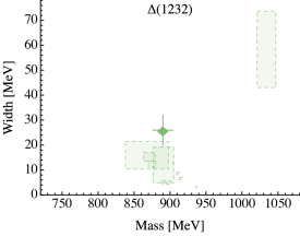
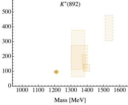
Figure 21: Current state in determination of certain hadronic resonances from lattice QCD, references can be found in the main text. Dashed/full boxes denote, respectively, the lattice driven determinations at unphysical/physical and near physical pion mass as discussed in the main text. The PDG [18] values are denoted by the diamonds with error bars.

In this review we have discussed the status of our theoretical understanding of hadron resonances. The main tools at our disposal are lattice QCD and effective field theories, which need to go hand in hand to make progress. In particular, for determining phase-shifts from lattice QCD the usage of finite-volume effective field theory (aka the Lüscher formalism) is mandatory. Once phase-shifts are determined it is again effective field theory to interpret this data and extract the resonance pole positions. HAL QCD has developed an alternative method to determine potentials from lattice QCD simulations.

There has been significant progress over the last years in lattice QCD, both methodologically and in practice for our understanding of QCD resonances. The best studied state is certainly the $\rho$-resonance, which is the only resonance for which a continuum extrapolation has been performed so far. However, the $\rho$ shows also the strongest pion mass dependence and, thus, a continuum extrapolation at physical pion mass values is likely required to finally compare to experiment. Also for the other well separated resonances $K^{\ast}(892)$, $\Delta(1232)$ and $f_{0}(500)$ there are now several lattice results available. For those the control of systematics is by far not as good as for the $\rho$-resonance. However, reasonable agreement with experiment is observed. All available estimates for mass and width of these four states are compiled in fig. 21. The figure nicely summarizes the status and the different levels of maturity of the lattice studies for the corresponding states. It also shows that baryon resonances are particularly challenging. We expect in the near future further results with ever more realistic simulation parameters for these four resonances.

Less well studied are resonances with strong effects from coupled channels or which are close to thresholds. This includes for instance light scalar mesons. However, the formalism for coupled channel analyses has been developed and also successfully applied, though still at unphysical parameter values. An example is the investigation by the Hadron Spectrum Collaboration of a coupled $\pi K$ and $\eta K$ system. Important lessons are learned about the interpolating operators that need to be included: in many cases multi-hadron operators are, not unexpectedly, mandatory. Also three pion resonant channels are being investigated in exploratory studies.

The Roper-resonance, despite significant effort, stays elusive: the inclusion of three-body interpolators, like for instance $\pi\pi N$, and the corresponding inelastic channels might provide a way out in the future.

Open and closed charm states represent another set of resonances relatively well covered in lattice studies. Most results are available for the $D_{s0}^{\ast}(2317)$ located a few MeV below the $DK$ threshold. Since it is very narrow, the energy difference to the $DK$ threshold is a meaningful quantity, and the available lattice determinations of it provide a consistent picture in agreement with experiment. For the $D_{0}^{\ast}(2300)$ fewer results are available, but it seems that it is located below the $D\pi$ threshold at large pion mass values, but moves above threshold towards physical pion mass values. Note that this state reveals a two-pole structure similar to the enigmatic $\Lambda(1405)$. Such two-pole structures should also be seen for the axial $D$ mesons and the corresponding $B$ mesons siblings, see, e.g., Ref. [292].

For the $X(3872)$ the two available estimates of the mass are about $15\ \mathrm{MeV}$ below the $D\bar{D}^{\ast}$ threshold. These investigations are both at way too large pion mass values, such that a comparison to the experimental $X(3872)$ energy level is not yet really meaningful. For the $Z_{c}(3900)$ on the other hand, a lattice study appears to be difficult: no definite candidate for this state could be identified unambiguously.

Concerning dibaryons, it is at present unclear whether such objects are really bound. In general, coupled channel analyses are required to be able to make definite conclusions, as prominently exhibited in case of the elusive $H$ dibaryon.

From all this it should have become clear that we are still far away from a detailed understanding of the hadron spectrum based on such first principles calculations. The results reported here are encouraging, as most of the required theoretical framework has been developed. As an important lesson, it has become clear that the choice of interpolating operators strongly influences the observed states. This means, on the one hand that the outcome of lattice investigations depends on the list of operators included. But on the other hand it gives hope that from the coupling of states to certain operators one can learn about the nature of the state. But, of course, it foremost means that a large list of operators need to be constructed, which was greatly simplified by methods like (stochastic) distillation, but is still very costly. Work is ongoing to further improve the operator construction, see for instance Ref. [494].

Another lesson one can learn from the existing investigations is that threshold effects can be misinterpreted as resonances. Here, a careful data analysis is required.

Finally, lattice artefacts and pion mass dependence can be significant. This can mean a bound state turns into a resonance or vice versa once the limits are studied properly.

In the future we, therefore, think that it will be important to further investigate the dependence of results on the list of operators, but also to better study continuum and chiral limits. A next important step will be to tackle three-body decays: in particular the $\omega$ meson and the Roper resonance in the baryon sector represent worthy targets.

References

- [1] W. Heisenberg, Physics and Beyond: Encounters and Conversations, Harper & Row, 1972.
- [2] R. F. Lebed, R. E. Mitchell, E. S. Swanson, Heavy-Quark QCD Exotica, Prog. Part. Nucl. Phys. 93 (2017) 143–194. arXiv:1610.04528, doi:10.1016/j.ppnp.2016.11.003.
- [3] A. Esposito, A. Pilloni, A. D. Polosa, Multiquark Resonances, Phys. Rept. 668 (2017) 1–97. arXiv:1611.07920, doi:10.1016/j.physrep.2016.11.002.
- [4] A. Hosaka, T. Iijima, K. Miyabayashi, Y. Sakai, S. Yasui, Exotic hadrons with heavy flavors: X, Y, Z, and related states, PTEP 2016 (6) (2016) 062C01. arXiv:1603.09229, doi:10.1093/ptep/ptw045.
- [5] H.-X. Chen, W. Chen, X. Liu, S.-L. Zhu, The hidden-charm pentaquark and tetraquark states, Phys. Rept. 639 (2016) 1–121. arXiv:1601.02092, doi:10.1016/j.physrep.2016.05.004.
- [6] H.-X. Chen, W. Chen, X. Liu, Y.-R. Liu, S.-L. Zhu, A review of the open charm and open bottom systems, Rept. Prog. Phys. 80 (7) (2017) 076201. arXiv:1609.08928, doi:10.1088/1361-6633/aa6420.
- [7] A. Ali, J. S. Lange, S. Stone, Exotics: Heavy Pentaquarks and Tetraquarks, Prog. Part. Nucl. Phys. 97 (2017) 123–198. arXiv:1706.00610, doi:10.1016/j.ppnp.2017.08.003.
- [8] F.-K. Guo, C. Hanhart, U.-G. Meißner, Q. Wang, Q. Zhao, B.-S. Zou, Hadronic molecules, Rev. Mod. Phys. 90 (1) (2018) 015004. arXiv:1705.00141, doi:10.1103/RevModPhys.90.015004.
- [9] S. L. Olsen, T. Skwarnicki, D. Zieminska, Nonstandard heavy mesons and baryons: Experimental evidence, Rev. Mod. Phys. 90 (1) (2018) 015003. arXiv:1708.04012, doi:10.1103/RevModPhys.90.015003.
- [10] M. Karliner, J. L. Rosner, T. Skwarnicki, Multiquark States, Ann. Rev. Nucl. Part. Sci. 68 (2018) 17–44. arXiv:1711.10626, doi:10.1146/annurev-nucl-101917-020902.
- [11] N. Brambilla, S. Eidelman, C. Hanhart, A. Nefediev, C.-P. Shen, C. E. Thomas, A. Vairo, C.-Z. Yuan, The states: experimental and theoretical status and perspectives, Phys. Rept. 873 (2020) 1–154. arXiv:1907.07583, doi:10.1016/j.physrep.2020.05.001.
- [12] Y.-R. Liu, H.-X. Chen, W. Chen, X. Liu, S.-L. Zhu, Pentaquark and Tetraquark states, Prog. Part. Nucl. Phys. 107 (2019) 237–320. arXiv:1903.11976, doi:10.1016/j.ppnp.2019.04.003.
- [13] A. Ali, L. Maiani, A. D. Polosa, Multiquark Hadrons, Cambridge University Press, 2019. doi:10.1017/9781316761465.
- [14] G. Yang, J. Ping, J. Segovia, Tetra- and penta-quark structures in the constituent quark model, Symmetry 12 (11) (2020) 1869. arXiv:2009.00238, doi:10.3390/sym12111869.
- [15] M. Albaladejo, et al., Novel approaches in Hadron SpectroscopyarXiv:2112.13436.
- [16] H.-X. Chen, W. Chen, X. Liu, Y.-R. Liu, S.-L. Zhu, An updated review of the new hadron statesarXiv:2204.02649.
- [17] N. Brambilla, et al., Substructure of Multiquark Hadrons (Snowmass 2021 White Paper)arXiv:2203.16583.
- [18] P. A. Zyla, et al., Review of Particle Physics, PTEP 2020 (8) (2020) 083C01. doi:10.1093/ptep/ptaa104.
- [19] E. P. Wigner, Resonance Reactions and Anomalous Scattering, Phys. Rev. 70 (1946) 15–33. doi:10.1103/PhysRev.70.15.
- [20] S. M. Flatte, Coupled - Channel Analysis of the pi eta and K anti-K Systems Near K anti-K Threshold, Phys. Lett. B 63 (1976) 224–227. doi:10.1016/0370-2693(76)90654-7.
- [21] L. Lesniak, Meson spectroscopy and separable potentials, Acta Phys. Polon. B 27 (1996) 1835–1847.
- [22] B. Kerbikov, A Remark on the effective range approach to the f0 - a0 mesons, Phys. Lett. B 596 (2004) 200–204. arXiv:hep-ph/0402022, doi:10.1016/j.physletb.2004.06.084.
- [23] V. Baru, J. Haidenbauer, C. Hanhart, A. E. Kudryavtsev, U.-G. Meißner, Flatte-like distributions and the a(0)(980) / f(0)(980) mesons, Eur. Phys. J. A 23 (2005) 523–533. arXiv:nucl-th/0410099, doi:10.1140/epja/i2004-10105-x.
- [24] P. Estabrooks, A. D. Martin, pi pi Phase Shift Analysis Below the K anti-K Threshold, Nucl. Phys. B 79 (1974) 301–316. doi:10.1016/0550-3213(74)90488-X.
- [25] S. D. Protopopescu, M. Alston-Garnjost, A. Barbaro-Galtieri, S. M. Flatte, J. H. Friedman, T. A. Lasinski, G. R. Lynch, M. S. Rabin, F. T. Solmitz, Pi pi Partial Wave Analysis from Reactions pi+ p — pi+ pi- Delta++ and pi+ p — K+ K- Delta++ at 7.1-GeV/c, Phys. Rev. D 7 (1973) 1279. doi:10.1103/PhysRevD.7.1279.
- [26] A. Zichichi, Subnuclear Phenomena, Academic Press, 1970.
- [27] D. Sadasivan, M. Mai, H. Akdag, M. Döring, Dalitz plots and lineshape of from a relativistic three-body unitary approach, Phys. Rev. D 101 (9) (2020) 094018, [Erratum: Phys.Rev.D 103, 019901 (2021)]. arXiv:2002.12431, doi:10.1103/PhysRevD.101.094018.
- [28] M. Mai, M. Döring, C. Granados, H. Haberzettl, U.-G. Meißner, D. Rönchen, I. Strakovsky, R. Workman, Jülich-Bonn-Washington model for pion electroproduction multipoles, Phys. Rev. C 103 (6) (2021) 065204. arXiv:2104.07312, doi:10.1103/PhysRevC.103.065204.
- [29] D. Severt, U.-G. Meißner, The Roper Resonance in a finite volume, Commun. Theor. Phys. 72 (7) (2020) 075201. arXiv:2003.05745, doi:10.1088/1572-9494/ab8a24.
- [30] W. Heisenberg, THE ’OBSERVABLE QUANTITIES’ IN THE THEORY OF ELEMENTARY PARTICLES.
- [31] N. G. van Kampen, S-Matrix and Causality Condition. I. Maxwell Field, Phys. Rev. 89 (1953) 1072–1079. doi:10.1103/PhysRev.89.1072.
- [32] G. Minerbo, Causality and analyticity in formal scattering theory, Phys. Rev. D 3 (1971) 928–932. doi:10.1103/PhysRevD.3.928.
- [33] R. J. Eden, P. V. Landshoff, D. I. Olive, J. C. Polkinghorne, The analytic S-matrix, Cambridge Univ. Press, Cambridge, 1966.
- [34] A. Cieply, E. Friedman, A. Gal, D. Gazda, J. Mares, K- nuclear potentials from in-medium chirally motivated models, Phys. Rev. C 84 (2011) 045206. arXiv:1108.1745, doi:10.1103/PhysRevC.84.045206.
- [35] A. Cieplý, M. Mai, U.-G. Meißner, J. Smejkal, On the pole content of coupled channels chiral approaches used for the system, Nucl. Phys. A 954 (2016) 17–40. arXiv:1603.02531, doi:10.1016/j.nuclphysa.2016.04.031.
- [36] D. Jido, J. A. Oller, E. Oset, A. Ramos, U.-G. Meißner, Chiral dynamics of the two Lambda(1405) states, Nucl. Phys. A 725 (2003) 181–200. arXiv:nucl-th/0303062, doi:10.1016/S0375-9474(03)01598-7.
- [37] M. Doring, C. Hanhart, F. Huang, S. Krewald, U. G. Meißner, Analytic properties of the scattering amplitude and resonances parameters in a meson exchange model, Nucl. Phys. A 829 (2009) 170–209. arXiv:0903.4337, doi:10.1016/j.nuclphysa.2009.08.010.
- [38] M. Mai, A. Alexandru, R. Brett, C. Culver, M. Döring, F. X. Lee, D. Sadasivan, Three-Body Dynamics of the a1(1260) Resonance from Lattice QCD, Phys. Rev. Lett. 127 (22) (2021) 222001. arXiv:2107.03973, doi:10.1103/PhysRevLett.127.222001.
- [39] D. Sadasivan, A. Alexandru, H. Akdag, F. Amorim, R. Brett, C. Culver, M. Döring, F. X. Lee, M. Mai, Pole position of the a1(1260) resonance in a three-body unitary framework, Phys. Rev. D 105 (5) (2022) 054020. arXiv:2112.03355, doi:10.1103/PhysRevD.105.054020.
- [40] D. Guo, A. Alexandru, R. Molina, M. Döring, Rho resonance parameters from lattice QCD, Phys. Rev. D 94 (3) (2016) 034501. arXiv:1605.03993, doi:10.1103/PhysRevD.94.034501.
- [41] D. Guo, A. Alexandru, R. Molina, M. Mai, M. Döring, Extraction of isoscalar phase-shifts from lattice QCD, Phys. Rev. D 98 (1) (2018) 014507. arXiv:1803.02897, doi:10.1103/PhysRevD.98.014507.
- [42] C. Culver, M. Mai, A. Alexandru, M. Döring, F. X. Lee, Pion scattering in the isospin channel from elongated lattices, Phys. Rev. D 100 (3) (2019) 034509. arXiv:1905.10202, doi:10.1103/PhysRevD.100.034509.
- [43] M. Mai, C. Culver, A. Alexandru, M. Döring, F. X. Lee, Cross-channel study of pion scattering from lattice QCD, Phys. Rev. D 100 (11) (2019) 114514. arXiv:1908.01847, doi:10.1103/PhysRevD.100.114514.
- [44] J. R. Pelaez, From controversy to precision on the sigma meson: a review on the status of the non-ordinary resonance, Phys. Rept. 658 (2016) 1. arXiv:1510.00653, doi:10.1016/j.physrep.2016.09.001.
- [45] A. Dobado, J. R. Pelaez, The Inverse amplitude method in chiral perturbation theory, Phys. Rev. D 56 (1997) 3057–3073. arXiv:hep-ph/9604416, doi:10.1103/PhysRevD.56.3057.
- [46] C. Hanhart, J. R. Pelaez, G. Rios, Quark mass dependence of the rho and sigma from dispersion relations and Chiral Perturbation Theory, Phys. Rev. Lett. 100 (2008) 152001. arXiv:0801.2871, doi:10.1103/PhysRevLett.100.152001.
-
[47]
A. Haar, Der massbegriff in der
theorie der kontinuierlichen gruppen, Annals of Mathematics 34 (1) (1933)
147–169.
URL http://www.jstor.org/stable/1968346 - [48] M. Lüscher, S. Schaefer, Lattice QCD with open boundary conditions and twisted-mass reweighting, Comput. Phys. Commun. 184 (2013) 519–528. arXiv:1206.2809, doi:10.1016/j.cpc.2012.10.003.
- [49] K. G. Wilson, Confinement of Quarks, Phys. Rev. D 10 (1974) 2445–2459. doi:10.1103/PhysRevD.10.2445.
- [50] P. Weisz, Continuum Limit Improved Lattice Action for Pure Yang-Mills Theory. 1., Nucl. Phys. B 212 (1983) 1–17. doi:10.1016/0550-3213(83)90595-3.
- [51] Y. Iwasaki, Renormalization Group Analysis of Lattice Theories and Improved Lattice Action: Two-Dimensional Nonlinear O(N) Sigma Model, Nucl. Phys. B 258 (1985) 141–156. doi:10.1016/0550-3213(85)90606-6.
- [52] J. B. Kogut, L. Susskind, Hamiltonian Formulation of Wilson’s Lattice Gauge Theories, Phys. Rev. D 11 (1975) 395–408. doi:10.1103/PhysRevD.11.395.
- [53] L. Susskind, Lattice Fermions, Phys. Rev. D 16 (1977) 3031–3039. doi:10.1103/PhysRevD.16.3031.
- [54] H. Neuberger, Exactly massless quarks on the lattice, Phys. Lett. B 417 (1998) 141–144. arXiv:hep-lat/9707022, doi:10.1016/S0370-2693(97)01368-3.
- [55] H. Neuberger, More about exactly massless quarks on the lattice, Phys. Lett. B 427 (1998) 353–355. arXiv:hep-lat/9801031, doi:10.1016/S0370-2693(98)00355-4.
- [56] D. B. Kaplan, A Method for simulating chiral fermions on the lattice, Phys. Lett. B 288 (1992) 342–347. arXiv:hep-lat/9206013, doi:10.1016/0370-2693(92)91112-M.
- [57] V. Furman, Y. Shamir, Axial symmetries in lattice QCD with Kaplan fermions, Nucl. Phys. B 439 (1995) 54–78. arXiv:hep-lat/9405004, doi:10.1016/0550-3213(95)00031-M.
- [58] M. Lüscher, Exact chiral symmetry on the lattice and the Ginsparg-Wilson relation, Phys. Lett. B 428 (1998) 342–345. arXiv:hep-lat/9802011, doi:10.1016/S0370-2693(98)00423-7.
- [59] C. J. Morningstar, M. J. Peardon, Efficient glueball simulations on anisotropic lattices, Phys. Rev. D 56 (1997) 4043–4061. arXiv:hep-lat/9704011, doi:10.1103/PhysRevD.56.4043.
- [60] B. Sheikholeslami, R. Wohlert, Improved Continuum Limit Lattice Action for QCD with Wilson Fermions, Nucl. Phys. B 259 (1985) 572. doi:10.1016/0550-3213(85)90002-1.
- [61] K. Jansen, C. Liu, Implementation of Symanzik’s improvement program for simulations of dynamical Wilson fermions in lattice QCD, Comput. Phys. Commun. 99 (1997) 221–234. arXiv:hep-lat/9603008, doi:10.1016/S0010-4655(96)00128-2.
- [62] M. Lüscher, S. Sint, R. Sommer, P. Weisz, U. Wolff, Nonperturbative O(a) improvement of lattice QCD, Nucl. Phys. B 491 (1997) 323–343. arXiv:hep-lat/9609035, doi:10.1016/S0550-3213(97)00080-1.
- [63] R. Frezzotti, P. A. Grassi, S. Sint, P. Weisz, A Local formulation of lattice QCD without unphysical fermion zero modes, Nucl. Phys. B Proc. Suppl. 83 (2000) 941–946. arXiv:hep-lat/9909003, doi:10.1016/S0920-5632(00)91852-8.
- [64] D. Becirevic, P. Boucaud, V. Lubicz, G. Martinelli, F. Mescia, S. Simula, C. Tarantino, Exploring twisted mass lattice QCD with the Clover term, Phys. Rev. D 74 (2006) 034501. arXiv:hep-lat/0605006, doi:10.1103/PhysRevD.74.034501.
- [65] R. Frezzotti, G. C. Rossi, Chirally improving Wilson fermions. 1. O(a) improvement, JHEP 08 (2004) 007. arXiv:hep-lat/0306014, doi:10.1088/1126-6708/2004/08/007.
- [66] C. Morningstar, M. J. Peardon, Analytic smearing of SU(3) link variables in lattice QCD, Phys. Rev. D 69 (2004) 054501. arXiv:hep-lat/0311018, doi:10.1103/PhysRevD.69.054501.
- [67] S. Capitani, S. Durr, C. Hoelbling, Rationale for UV-filtered clover fermions, JHEP 11 (2006) 028. arXiv:hep-lat/0607006, doi:10.1088/1126-6708/2006/11/028.
- [68] M. Lüscher, Construction of a Selfadjoint, Strictly Positive Transfer Matrix for Euclidean Lattice Gauge Theories, Commun. Math. Phys. 54 (1977) 283. doi:10.1007/BF01614090.
- [69] K. Osterwalder, R. Schrader, AXIOMS FOR EUCLIDEAN GREEN’S FUNCTIONS, Commun. Math. Phys. 31 (1973) 83–112. doi:10.1007/BF01645738.
- [70] K. Osterwalder, R. Schrader, Axioms for Euclidean Green’s Functions. 2., Commun. Math. Phys. 42 (1975) 281. doi:10.1007/BF01608978.
- [71] A. Alexandru, R. Brett, C. Culver, M. Döring, D. Guo, F. X. Lee, M. Mai, Finite-volume energy spectrum of the system, Phys. Rev. D 102 (11) (2020) 114523. arXiv:2009.12358, doi:10.1103/PhysRevD.102.114523.
- [72] A. X. El-Khadra, A. S. Kronfeld, P. B. Mackenzie, Massive fermions in lattice gauge theory, Phys. Rev. D 55 (1997) 3933–3957. arXiv:hep-lat/9604004, doi:10.1103/PhysRevD.55.3933.
- [73] B. Blossier, et al., A Proposal for B-physics on current lattices, JHEP 04 (2010) 049. arXiv:0909.3187, doi:10.1007/JHEP04(2010)049.
- [74] L. Maiani, M. Testa, Final state interactions from Euclidean correlation functions, Phys. Lett. B 245 (1990) 585–590. doi:10.1016/0370-2693(90)90695-3.
-
[75]
B. S. DeWitt,
Transition from
discrete to continuous spectra, Phys. Rev. 103 (1956) 1565–1571.
doi:10.1103/PhysRev.103.1565.
URL https://link.aps.org/doi/10.1103/PhysRev.103.1565 -
[76]
K. Huang, C. N. Yang,
Quantum-mechanical
many-body problem with hard-sphere interaction, Phys. Rev. 105 (1957)
767–775.
doi:10.1103/PhysRev.105.767.
URL https://link.aps.org/doi/10.1103/PhysRev.105.767 - [77] M. Lüscher, Volume Dependence of the Energy Spectrum in Massive Quantum Field Theories. 2. Scattering States, Commun. Math. Phys. 105 (1986) 153–188. doi:10.1007/BF01211097.
- [78] M. Lüscher, Two particle states on a torus and their relation to the scattering matrix, Nucl. Phys. B 354 (1991) 531–578. doi:10.1016/0550-3213(91)90366-6.
- [79] J. Gasser, H. Leutwyler, Light Quarks at Low Temperatures, Phys. Lett. B 184 (1987) 83–88. doi:10.1016/0370-2693(87)90492-8.
- [80] J. Gasser, H. Leutwyler, Thermodynamics of Chiral Symmetry, Phys. Lett. B 188 (1987) 477–481. doi:10.1016/0370-2693(87)91652-2.
- [81] R. A. Briceno, J. J. Dudek, R. D. Young, Scattering processes and resonances from lattice QCD, Rev. Mod. Phys. 90 (2) (2018) 025001. arXiv:1706.06223, doi:10.1103/RevModPhys.90.025001.
- [82] C. Morningstar, J. Bulava, B. Singha, R. Brett, J. Fallica, A. Hanlon, B. Hörz, Estimating the two-particle -matrix for multiple partial waves and decay channels from finite-volume energies, Nucl. Phys. B 924 (2017) 477–507. arXiv:1707.05817, doi:10.1016/j.nuclphysb.2017.09.014.
- [83] F. X. Lee, A. Alexandru, R. Brett, Validation of the finite-volume quantization condition for two spinless particlesarXiv:2107.04430.
- [84] K. Polejaeva, A. Rusetsky, Three particles in a finite volume, Eur. Phys. J. A 48 (2012) 67. arXiv:1203.1241, doi:10.1140/epja/i2012-12067-8.
- [85] M. Mai, M. Döring, Three-body Unitarity in the Finite Volume, Eur. Phys. J. A 53 (12) (2017) 240. arXiv:1709.08222, doi:10.1140/epja/i2017-12440-1.
- [86] M. Mai, M. Doring, Finite-Volume Spectrum of and Systems, Phys. Rev. Lett. 122 (6) (2019) 062503. arXiv:1807.04746, doi:10.1103/PhysRevLett.122.062503.
- [87] M. Mai, M. Döring, C. Culver, A. Alexandru, Three-body unitarity versus finite-volume spectrum from lattice QCD, Phys. Rev. D 101 (5) (2020) 054510. arXiv:1909.05749, doi:10.1103/PhysRevD.101.054510.
- [88] C. Culver, M. Mai, R. Brett, A. Alexandru, M. Döring, Three pion spectrum in the channel from lattice QCD, Phys. Rev. D 101 (11) (2020) 114507. arXiv:1911.09047, doi:10.1103/PhysRevD.101.114507.
- [89] M. Döring, H. W. Hammer, M. Mai, J. Y. Pang, t. A. Rusetsky, J. Wu, Three-body spectrum in a finite volume: the role of cubic symmetry, Phys. Rev. D 97 (11) (2018) 114508. arXiv:1802.03362, doi:10.1103/PhysRevD.97.114508.
- [90] R. A. Briceño, M. T. Hansen, S. R. Sharpe, Three-particle systems with resonant subprocesses in a finite volume, Phys. Rev. D 99 (1) (2019) 014516. arXiv:1810.01429, doi:10.1103/PhysRevD.99.014516.
- [91] T. D. Blanton, F. Romero-López, S. R. Sharpe, Implementing the three-particle quantization condition including higher partial waves, JHEP 03 (2019) 106. arXiv:1901.07095, doi:10.1007/JHEP03(2019)106.
- [92] R. A. Briceño, M. T. Hansen, S. R. Sharpe, A. P. Szczepaniak, Unitarity of the infinite-volume three-particle scattering amplitude arising from a finite-volume formalism, Phys. Rev. D 100 (5) (2019) 054508. arXiv:1905.11188, doi:10.1103/PhysRevD.100.054508.
- [93] A. W. Jackura, S. M. Dawid, C. Fernández-Ramírez, V. Mathieu, M. Mikhasenko, A. Pilloni, S. R. Sharpe, A. P. Szczepaniak, Equivalence of three-particle scattering formalisms, Phys. Rev. D 100 (3) (2019) 034508. arXiv:1905.12007, doi:10.1103/PhysRevD.100.034508.
- [94] R. Brett, C. Culver, M. Mai, A. Alexandru, M. Döring, F. X. Lee, Three-body interactions from the finite-volume QCD spectrum, Phys. Rev. D 104 (1) (2021) 014501. arXiv:2101.06144, doi:10.1103/PhysRevD.104.014501.
- [95] F. Romero-López, S. R. Sharpe, T. D. Blanton, R. A. Briceño, M. T. Hansen, Numerical exploration of three relativistic particles in a finite volume including two-particle resonances and bound states, JHEP 10 (2019) 007. arXiv:1908.02411, doi:10.1007/JHEP10(2019)007.
- [96] J.-Y. Pang, J.-J. Wu, H. W. Hammer, U.-G. Meißner, A. Rusetsky, Energy shift of the three-particle system in a finite volume, Phys. Rev. D 99 (7) (2019) 074513. arXiv:1902.01111, doi:10.1103/PhysRevD.99.074513.
- [97] T. D. Blanton, S. R. Sharpe, Equivalence of relativistic three-particle quantization conditions, Phys. Rev. D 102 (5) (2020) 054515. arXiv:2007.16190, doi:10.1103/PhysRevD.102.054515.
- [98] F. Müller, A. Rusetsky, On the three-particle analog of the Lellouch-Lüscher formula, JHEP 03 (2021) 152. arXiv:2012.13957, doi:10.1007/JHEP03(2021)152.
- [99] F. Müller, J.-Y. Pang, A. Rusetsky, J.-J. Wu, Relativistic-invariant formulation of the NREFT three-particle quantization condition, JHEP 02 (2022) 158. arXiv:2110.09351, doi:10.1007/JHEP02(2022)158.
- [100] M. T. Hansen, F. Romero-López, S. R. Sharpe, Decay amplitudes to three hadrons from finite-volume matrix elements, JHEP 04 (2021) 113. arXiv:2101.10246, doi:10.1007/JHEP04(2021)113.
- [101] T. D. Blanton, S. R. Sharpe, Three-particle finite-volume formalism for ++K+ and related systems, Phys. Rev. D 104 (3) (2021) 034509. arXiv:2105.12094, doi:10.1103/PhysRevD.104.034509.
- [102] T. D. Blanton, F. Romero-López, S. R. Sharpe, Implementing the three-particle quantization condition for ++K+ and related systems, JHEP 02 (2022) 098. arXiv:2111.12734, doi:10.1007/JHEP02(2022)098.
- [103] P. Guo, B. Long, Multi- systems in a finite volume, Phys. Rev. D 101 (9) (2020) 094510. arXiv:2002.09266, doi:10.1103/PhysRevD.101.094510.
- [104] P. Guo, Modeling few-body resonances in finite volume, Phys. Rev. D 102 (5) (2020) 054514. arXiv:2007.12790, doi:10.1103/PhysRevD.102.054514.
- [105] P. Guo, Threshold expansion formula of bosons in a finite volume from a variational approach, Phys. Rev. D 101 (5) (2020) 054512. arXiv:2002.04111, doi:10.1103/PhysRevD.101.054512.
- [106] P. Guo, B. Long, Visualizing resonances in finite volume, Phys. Rev. D 102 (7) (2020) 074508. arXiv:2007.10895, doi:10.1103/PhysRevD.102.074508.
- [107] M. T. Hansen, S. R. Sharpe, Lattice QCD and Three-particle Decays of Resonances, Ann. Rev. Nucl. Part. Sci. 69 (2019) 65–107. arXiv:1901.00483, doi:10.1146/annurev-nucl-101918-023723.
- [108] M. Mai, M. Döring, A. Rusetsky, Multi-particle systems on the lattice and chiral extrapolations: a brief review, Eur. Phys. J. ST 230 (6) (2021) 1623–1643. arXiv:2103.00577, doi:10.1140/epjs/s11734-021-00146-5.
- [109] K. Rummukainen, S. A. Gottlieb, Resonance scattering phase shifts on a nonrest frame lattice, Nucl. Phys. B 450 (1995) 397–436. arXiv:hep-lat/9503028, doi:10.1016/0550-3213(95)00313-H.
- [110] D. C. Moore, G. T. Fleming, Angular momentum on the lattice: The Case of non-zero linear momentum, Phys. Rev. D 73 (2006) 014504, [Erratum: Phys.Rev.D 74, 079905 (2006)]. arXiv:hep-lat/0507018, doi:10.1103/PhysRevD.73.014504.
- [111] X. Feng, K. Jansen, D. B. Renner, Resonance Parameters of the rho-Meson from Lattice QCD, Phys. Rev. D 83 (2011) 094505. arXiv:1011.5288, doi:10.1103/PhysRevD.83.094505.
- [112] R. A. Briceno, Two-particle multichannel systems in a finite volume with arbitrary spin, Phys. Rev. D 89 (7) (2014) 074507. arXiv:1401.3312, doi:10.1103/PhysRevD.89.074507.
- [113] V. Bernard, M. Lage, U.-G. Meißner, A. Rusetsky, Resonance properties from the finite-volume energy spectrum, JHEP 08 (2008) 024. arXiv:0806.4495, doi:10.1088/1126-6708/2008/08/024.
- [114] M. Gockeler, R. Horsley, M. Lage, U. G. Meißner, P. E. L. Rakow, A. Rusetsky, G. Schierholz, J. M. Zanotti, Scattering phases for meson and baryon resonances on general moving-frame lattices, Phys. Rev. D 86 (2012) 094513. arXiv:1206.4141, doi:10.1103/PhysRevD.86.094513.
- [115] J. J. Dudek, R. G. Edwards, C. E. Thomas, S and D-wave phase shifts in isospin-2 pi pi scattering from lattice QCD, Phys. Rev. D 86 (2012) 034031. arXiv:1203.6041, doi:10.1103/PhysRevD.86.034031.
- [116] C. McNeile, C. Michael, P. Pennanen, Hybrid meson decay from the lattice, Phys. Rev. D 65 (2002) 094505. arXiv:hep-lat/0201006, doi:10.1103/PhysRevD.65.094505.
- [117] C. McNeile, C. Michael, Hadronic decay of a vector meson from the lattice, Phys. Lett. B 556 (2003) 177–184. arXiv:hep-lat/0212020, doi:10.1016/S0370-2693(03)00130-8.
- [118] C. Alexandrou, J. W. Negele, M. Petschlies, A. Strelchenko, A. Tsapalis, Determination of Resonance Parameters from Lattice QCD, Phys. Rev. D 88 (3) (2013) 031501. arXiv:1305.6081, doi:10.1103/PhysRevD.88.031501.
- [119] C. McNeile, C. Michael, Mixing of scalar glueballs and flavor singlet scalar mesons, Phys. Rev. D 63 (2001) 114503. arXiv:hep-lat/0010019, doi:10.1103/PhysRevD.63.114503.
- [120] N. Ishii, S. Aoki, T. Hatsuda, The Nuclear Force from Lattice QCD, Phys. Rev. Lett. 99 (2007) 022001. arXiv:nucl-th/0611096, doi:10.1103/PhysRevLett.99.022001.
- [121] S. Aoki, T. Hatsuda, N. Ishii, Theoretical Foundation of the Nuclear Force in QCD and its applications to Central and Tensor Forces in Quenched Lattice QCD Simulations, Prog. Theor. Phys. 123 (2010) 89–128. arXiv:0909.5585, doi:10.1143/PTP.123.89.
- [122] S. Aoki, T. Doi, T. Hatsuda, Y. Ikeda, T. Inoue, N. Ishii, K. Murano, H. Nemura, K. Sasaki, Lattice QCD approach to Nuclear Physics, PTEP 2012 (2012) 01A105. arXiv:1206.5088, doi:10.1093/ptep/pts010.
- [123] S. Aoki, B. Charron, T. Doi, T. Hatsuda, T. Inoue, N. Ishii, Construction of energy-independent potentials above inelastic thresholds in quantum field theories, Phys. Rev. D 87 (3) (2013) 034512. arXiv:1212.4896, doi:10.1103/PhysRevD.87.034512.
- [124] T. Iritani, S. Aoki, T. Doi, S. Gongyo, T. Hatsuda, Y. Ikeda, T. Inoue, N. Ishii, H. Nemura, K. Sasaki, Systematics of the HAL QCD Potential at Low Energies in Lattice QCD, Phys. Rev. D 99 (1) (2019) 014514. arXiv:1805.02365, doi:10.1103/PhysRevD.99.014514.
- [125] B. S. DeWitt, Transition from discrete to continuous spectra, Phys. Rev. 103 (1956) 1565–1571. doi:10.1103/PhysRev.103.1565.
- [126] D. Agadjanov, M. Doring, M. Mai, U.-G. Meißner, A. Rusetsky, The Optical Potential on the Lattice, JHEP 06 (2016) 043. arXiv:1603.07205, doi:10.1007/JHEP06(2016)043.
- [127] M. T. Hansen, H. B. Meyer, D. Robaina, From deep inelastic scattering to heavy-flavor semileptonic decays: Total rates into multihadron final states from lattice QCD, Phys. Rev. D 96 (9) (2017) 094513. arXiv:1704.08993, doi:10.1103/PhysRevD.96.094513.
- [128] R. A. Briceño, J. V. Guerrero, M. T. Hansen, A. M. Sturzu, Role of boundary conditions in quantum computations of scattering observables, Phys. Rev. D 103 (1) (2021) 014506. arXiv:2007.01155, doi:10.1103/PhysRevD.103.014506.
- [129] J. Bulava, M. T. Hansen, Scattering amplitudes from finite-volume spectral functions, Phys. Rev. D 100 (3) (2019) 034521. arXiv:1903.11735, doi:10.1103/PhysRevD.100.034521.
- [130] C. Michael, I. Teasdale, Extracting Glueball Masses From Lattice QCD, Nucl. Phys. B 215 (1983) 433–446. doi:10.1016/0550-3213(83)90674-0.
- [131] M. Lüscher, U. Wolff, How to Calculate the Elastic Scattering Matrix in Two-dimensional Quantum Field Theories by Numerical Simulation, Nucl. Phys. B 339 (1990) 222–252. doi:10.1016/0550-3213(90)90540-T.
- [132] B. Blossier, M. Della Morte, G. von Hippel, T. Mendes, R. Sommer, On the generalized eigenvalue method for energies and matrix elements in lattice field theory, JHEP 04 (2009) 094. arXiv:0902.1265, doi:10.1088/1126-6708/2009/04/094.
- [133] M. Fischer, B. Kostrzewa, J. Ostmeyer, K. Ottnad, M. Ueding, C. Urbach, On the generalised eigenvalue method and its relation to Prony and generalised pencil of function methods, Eur. Phys. J. A 56 (8) (2020) 206. arXiv:2004.10472, doi:10.1140/epja/s10050-020-00205-w.
- [134] M. Peardon, J. Bulava, J. Foley, C. Morningstar, J. Dudek, R. G. Edwards, B. Joo, H.-W. Lin, D. G. Richards, K. J. Juge, A Novel quark-field creation operator construction for hadronic physics in lattice QCD, Phys. Rev. D 80 (2009) 054506. arXiv:0905.2160, doi:10.1103/PhysRevD.80.054506.
- [135] C. Morningstar, J. Bulava, J. Foley, K. J. Juge, D. Lenkner, M. Peardon, C. H. Wong, Improved stochastic estimation of quark propagation with Laplacian Heaviside smearing in lattice QCD, Phys. Rev. D 83 (2011) 114505. arXiv:1104.3870, doi:10.1103/PhysRevD.83.114505.
- [136] R. Sommer, Scale setting in lattice QCD, PoS LATTICE2013 (2014) 015. arXiv:1401.3270, doi:10.22323/1.187.0015.
- [137] J. Gasser, H. Leutwyler, Chiral Perturbation Theory to One Loop, Annals Phys. 158 (1984) 142. doi:10.1016/0003-4916(84)90242-2.
- [138] J. Gasser, H. Leutwyler, Chiral Perturbation Theory: Expansions in the Mass of the Strange Quark, Nucl. Phys. B 250 (1985) 465–516. doi:10.1016/0550-3213(85)90492-4.
- [139] Y. Aoki, et al., FLAG Review 2021arXiv:2111.09849.
- [140] M. Albaladejo, J. A. Oller, E. Oset, G. Rios, L. Roca, Finite volume treatment of pi pi scattering and limits to phase shifts extraction from lattice QCD, JHEP 08 (2012) 071. arXiv:1205.3582, doi:10.1007/JHEP08(2012)071.
- [141] F. Romero-López, A. Rusetsky, C. Urbach, Two- and three-body interactions in theory from lattice simulations, Eur. Phys. J. C 78 (10) (2018) 846. arXiv:1806.02367, doi:10.1140/epjc/s10052-018-6325-8.
- [142] D. J. Wilson, R. A. Briceno, J. J. Dudek, R. G. Edwards, C. E. Thomas, Coupled scattering in -wave and the resonance from lattice QCD, Phys. Rev. D 92 (9) (2015) 094502. arXiv:1507.02599, doi:10.1103/PhysRevD.92.094502.
- [143] M. Padmanath, C. B. Lang, L. Leskovec, S. Prelovsek, scattering in the Roper channel, EPJ Web Conf. 175 (2018) 05004. arXiv:1711.06334, doi:10.1051/epjconf/201817505004.
- [144] K. Ottnad, C. Urbach, Flavor-singlet meson decay constants from twisted mass lattice QCD, Phys. Rev. D 97 (5) (2018) 054508. arXiv:1710.07986, doi:10.1103/PhysRevD.97.054508.
- [145] P. Dimopoulos, et al., Topological susceptibility and meson mass from lattice QCD at the physical point, Phys. Rev. D 99 (3) (2019) 034511. arXiv:1812.08787, doi:10.1103/PhysRevD.99.034511.
- [146] C. Helmes, C. Jost, B. Knippschild, B. Kostrzewa, L. Liu, F. Pittler, C. Urbach, M. Werner, Hadron-Hadron Interactions from Lattice QCD: Scattering Length, Phys. Rev. D 98 (11) (2018) 114511. arXiv:1809.08886, doi:10.1103/PhysRevD.98.114511.
- [147] U. J. Wiese, Identification of Resonance Parameters From the Finite Volume Energy Spectrum, Nucl. Phys. B Proc. Suppl. 9 (1989) 609–613. doi:10.1016/0920-5632(89)90171-0.
- [148] S. Weinberg, Phenomenological Lagrangians, Physica A 96 (1-2) (1979) 327–340. doi:10.1016/0378-4371(79)90223-1.
- [149] U. G. Meißner, Recent developments in chiral perturbation theory, Rept. Prog. Phys. 56 (1993) 903–996. arXiv:hep-ph/9302247, doi:10.1088/0034-4885/56/8/001.
- [150] G. Ecker, Chiral perturbation theory, Prog. Part. Nucl. Phys. 35 (1995) 1–80. arXiv:hep-ph/9501357, doi:10.1016/0146-6410(95)00041-G.
- [151] A. Pich, Chiral perturbation theory, Rept. Prog. Phys. 58 (1995) 563–610. arXiv:hep-ph/9502366, doi:10.1088/0034-4885/58/6/001.
- [152] V. Bernard, U.-G. Meißner, Chiral perturbation theory, Ann. Rev. Nucl. Part. Sci. 57 (2007) 33–60. arXiv:hep-ph/0611231, doi:10.1146/annurev.nucl.56.080805.140449.
- [153] J. Bijnens, Chiral perturbation theory beyond one loop, Prog. Part. Nucl. Phys. 58 (2007) 521–586. arXiv:hep-ph/0604043, doi:10.1016/j.ppnp.2006.08.002.
- [154] B. R. Holstein, Chiral perturbation theory: An effective field theory, Prog. Part. Nucl. Phys. 61 (2008) 3–18. doi:10.1016/j.ppnp.2007.12.007.
- [155] N. Hermansson-Truedsson, Chiral Perturbation Theory at NNNLO, Symmetry 12 (8) (2020) 1262. arXiv:2006.01430, doi:10.3390/sym12081262.
- [156] J. Gasser, M. E. Sainio, A. Svarc, Nucleons with Chiral Loops, Nucl. Phys. B 307 (1988) 779–853. doi:10.1016/0550-3213(88)90108-3.
- [157] E. E. Jenkins, A. V. Manohar, Baryon chiral perturbation theory using a heavy fermion Lagrangian, Phys. Lett. B 255 (1991) 558–562. doi:10.1016/0370-2693(91)90266-S.
- [158] V. Bernard, N. Kaiser, J. Kambor, U. G. Meißner, Chiral structure of the nucleon, Nucl. Phys. B 388 (1992) 315–345. doi:10.1016/0550-3213(92)90615-I.
- [159] V. Bernard, N. Kaiser, U.-G. Meißner, Chiral dynamics in nucleons and nuclei, Int. J. Mod. Phys. E 4 (1995) 193–346. arXiv:hep-ph/9501384, doi:10.1142/S0218301395000092.
- [160] S. Scherer, Chiral Perturbation Theory: Introduction and Recent Results in the One-Nucleon Sector, Prog. Part. Nucl. Phys. 64 (2010) 1–60. arXiv:0908.3425, doi:10.1016/j.ppnp.2009.08.002.
- [161] L. Geng, Recent developments in SU(3) covariant baryon chiral perturbation theory, Front. Phys. (Beijing) 8 (2013) 328–348. arXiv:1301.6815, doi:10.1007/s11467-013-0327-7.
- [162] A. Manohar, H. Georgi, Chiral Quarks and the Nonrelativistic Quark Model, Nucl. Phys. B 234 (1984) 189–212. doi:10.1016/0550-3213(84)90231-1.
- [163] T. N. Truong, Chiral Perturbation Theory and Final State Theorem, Phys. Rev. Lett. 61 (1988) 2526. doi:10.1103/PhysRevLett.61.2526.
- [164] A. Dobado, M. J. Herrero, T. N. Truong, Unitarized Chiral Perturbation Theory for Elastic Pion-Pion Scattering, Phys. Lett. B 235 (1990) 134–140. doi:10.1016/0370-2693(90)90109-J.
- [165] J. Gasser, U. G. Meißner, Chiral expansion of pion form-factors beyond one loop, Nucl. Phys. B 357 (1991) 90–128. doi:10.1016/0550-3213(91)90460-F.
- [166] I. Caprini, G. Colangelo, H. Leutwyler, Mass and width of the lowest resonance in QCD, Phys. Rev. Lett. 96 (2006) 132001. arXiv:hep-ph/0512364, doi:10.1103/PhysRevLett.96.132001.
- [167] J. R. Peláez, A. Rodas, J. R. de Elvira, Precision dispersive approaches versus unitarized chiral perturbation theory for the lightest scalar resonances and , Eur. Phys. J. ST 230 (6) (2021) 1539–1574. arXiv:2101.06506, doi:10.1140/epjs/s11734-021-00142-9.
- [168] P. C. Bruns, U.-G. Meißner, Infrared regularization for spin-1 fields, Eur. Phys. J. C 40 (2005) 97–119. arXiv:hep-ph/0411223, doi:10.1140/epjc/s2005-02118-0.
- [169] P. J. Ellis, H.-B. Tang, Pion nucleon scattering in a new approach to chiral perturbation theory, Phys. Rev. C 57 (1998) 3356–3375. arXiv:hep-ph/9709354, doi:10.1103/PhysRevC.57.3356.
- [170] J. Gegelia, G. S. Japaridze, K. S. Turashvili, Calculation of loop integrals by dimensional counting, Theor. Math. Phys. 101 (1994) 1313–1319. doi:10.1007/BF01018279.
- [171] M. Beneke, V. A. Smirnov, Asymptotic expansion of Feynman integrals near threshold, Nucl. Phys. B 522 (1998) 321–344. arXiv:hep-ph/9711391, doi:10.1016/S0550-3213(98)00138-2.
- [172] J. Bijnens, P. Gosdzinsky, P. Talavera, Matching the heavy vector meson theory, JHEP 01 (1998) 014. arXiv:hep-ph/9708232, doi:10.1088/1126-6708/1998/01/014.
- [173] E. E. Jenkins, A. V. Manohar, M. B. Wise, Chiral perturbation theory for vector mesons, Phys. Rev. Lett. 75 (1995) 2272–2275. arXiv:hep-ph/9506356, doi:10.1103/PhysRevLett.75.2272.
- [174] J. Bijnens, P. Gosdzinsky, Electromagnetic contributions to vector meson masses and mixings, Phys. Lett. B 388 (1996) 203–210. arXiv:hep-ph/9607462, doi:10.1016/0370-2693(96)01147-1.
- [175] J. Bijnens, P. Gosdzinsky, P. Talavera, Vector meson masses in chiral perturbation theory, Nucl. Phys. B 501 (1997) 495–517. arXiv:hep-ph/9704212, doi:10.1016/S0550-3213(97)00391-X.
- [176] P. D. Ruiz-Femenia, A. Pich, J. Portoles, Odd intrinsic parity processes within the resonance effective theory of QCD, JHEP 07 (2003) 003. arXiv:hep-ph/0306157, doi:10.1088/1126-6708/2003/07/003.
- [177] I. Rosell, J. J. Sanz-Cillero, A. Pich, Quantum loops in the resonance chiral theory: The Vector form-factor, JHEP 08 (2004) 042. arXiv:hep-ph/0407240, doi:10.1088/1126-6708/2004/08/042.
- [178] M. F. M. Lutz, S. Leupold, On the radiative decays of light vector and axial-vector mesons, Nucl. Phys. A 813 (2008) 96–170. arXiv:0801.3821, doi:10.1016/j.nuclphysa.2008.09.005.
- [179] P. C. Bruns, U.-G. Meißner, Infrared regularization with vector mesons and baryons, Eur. Phys. J. C 58 (2008) 407–422. arXiv:0808.3174, doi:10.1140/epjc/s10052-008-0775-3.
- [180] C. Terschlüsen, S. Leupold, M. F. M. Lutz, Electromagnetic Transitions in an Effective Chiral Lagrangian with the and Light Vector Mesons, Eur. Phys. J. A 48 (2012) 190. arXiv:1204.4125, doi:10.1140/epja/i2012-12190-6.
- [181] R. G. Stuart, Gauge invariance, analyticity and physical observables at the Z0 resonance, Phys. Lett. B 262 (1991) 113–119. doi:10.1016/0370-2693(91)90653-8.
- [182] A. Denner, S. Dittmaier, M. Roth, D. Wackeroth, Predictions for all processes e+ e- — 4 fermions + gamma, Nucl. Phys. B 560 (1999) 33–65. arXiv:hep-ph/9904472, doi:10.1016/S0550-3213(99)00437-X.
- [183] D. Djukanovic, J. Gegelia, A. Keller, S. Scherer, Complex-mass renormalization in chiral effective field theory, Phys. Lett. B 680 (2009) 235–238. arXiv:0902.4347, doi:10.1016/j.physletb.2009.08.068.
- [184] A. Denner, S. Dittmaier, The Complex-mass scheme for perturbative calculations with unstable particles, Nucl. Phys. B Proc. Suppl. 160 (2006) 22–26. arXiv:hep-ph/0605312, doi:10.1016/j.nuclphysbps.2006.09.025.
- [185] W. Beenakker, A. Denner, Infrared Divergent Scalar Box Integrals With Applications in the Electroweak Standard Model, Nucl. Phys. B 338 (1990) 349–370. doi:10.1016/0550-3213(90)90636-R.
- [186] A. Denner, J.-N. Lang, The Complex-Mass Scheme and Unitarity in perturbative Quantum Field Theory, Eur. Phys. J. C 75 (8) (2015) 377. arXiv:1406.6280, doi:10.1140/epjc/s10052-015-3579-2.
- [187] T. Becher, H. Leutwyler, Baryon chiral perturbation theory in manifestly Lorentz invariant form, Eur. Phys. J. C 9 (1999) 643–671. arXiv:hep-ph/9901384, doi:10.1007/PL00021673.
- [188] T. Fuchs, J. Gegelia, G. Japaridze, S. Scherer, Renormalization of relativistic baryon chiral perturbation theory and power counting, Phys. Rev. D 68 (2003) 056005. arXiv:hep-ph/0302117, doi:10.1103/PhysRevD.68.056005.
- [189] M. Gell-Mann, D. Sharp, W. G. Wagner, Decay rates of neutral mesons, Phys. Rev. Lett. 8 (1962) 261. doi:10.1103/PhysRevLett.8.261.
- [190] U. G. Meißner, Low-Energy Hadron Physics from Effective Chiral Lagrangians with Vector Mesons, Phys. Rept. 161 (1988) 213. doi:10.1016/0370-1573(88)90090-7.
- [191] M. Bando, T. Kugo, K. Yamawaki, Nonlinear Realization and Hidden Local Symmetries, Phys. Rept. 164 (1988) 217–314. doi:10.1016/0370-1573(88)90019-1.
- [192] G. Ecker, J. Gasser, H. Leutwyler, A. Pich, E. de Rafael, Chiral Lagrangians for Massive Spin 1 Fields, Phys. Lett. B 223 (1989) 425–432. doi:10.1016/0370-2693(89)91627-4.
- [193] K. Kawarabayashi, M. Suzuki, Partially conserved axial vector current and the decays of vector mesons, Phys. Rev. Lett. 16 (1966) 255. doi:10.1103/PhysRevLett.16.255.
- [194] Riazuddin, Fayyazuddin, Algebra of current components and decay widths of rho and K* mesons, Phys. Rev. 147 (1966) 1071–1073. doi:10.1103/PhysRev.147.1071.
- [195] R. Urech, rho0 - omega mixing in chiral perturbation theory, Phys. Lett. B 355 (1995) 308–312. arXiv:hep-ph/9504238, doi:10.1016/0370-2693(95)00749-B.
- [196] A. Gokalp, A. Kucukarslan, O. Yilmaz, VMD, chiral loops, sigma meson, and omega - rho mixing in omega — pi0 pi0 gamma decay, Phys. Rev. D 67 (2003) 073008. arXiv:hep-ph/0302240, doi:10.1103/PhysRevD.67.073008.
- [197] A. Kucukarslan, U.-G. Meißner, Omega-phi mixing in chiral perturbation theory, Mod. Phys. Lett. A 21 (2006) 1423–1430. arXiv:hep-ph/0603061, doi:10.1142/S0217732306020743.
- [198] Y.-H. Chen, D.-L. Yao, H.-Q. Zheng, A study of mixing in resonance chiral theory, Commun. Theor. Phys. 69 (1) (2018) 50. arXiv:1710.11448, doi:10.1088/0253-6102/69/1/50.
- [199] H. B. O’Connell, B. C. Pearce, A. W. Thomas, A. G. Williams, mixing, vector meson dominance and the pion form-factor, Prog. Part. Nucl. Phys. 39 (1997) 201–252. arXiv:hep-ph/9501251, doi:10.1016/S0146-6410(97)00044-6.
- [200] D. B. Leinweber, A. W. Thomas, K. Tsushima, S. V. Wright, Chiral behavior of the rho meson in lattice QCD, Phys. Rev. D 64 (2001) 094502. arXiv:hep-lat/0104013, doi:10.1103/PhysRevD.64.094502.
- [201] D. Djukanovic, M. R. Schindler, J. Gegelia, S. Scherer, Quantum electrodynamics for vector mesons, Phys. Rev. Lett. 95 (2005) 012001. arXiv:hep-ph/0505180, doi:10.1103/PhysRevLett.95.012001.
- [202] D. Djukanovic, J. Gegelia, A. Keller, S. Scherer, L. Tiator, Vector form factor of the pion in chiral effective field theory, Phys. Lett. B 742 (2015) 55–60. arXiv:1410.3801, doi:10.1016/j.physletb.2015.01.007.
- [203] D. Djukanovic, E. Epelbaum, J. Gegelia, H. Krebs, U. G. Meißner, Complex-mass renormalization in hadronic EFT: applicability at two-loop order, Eur. Phys. J. A 51 (2015) 101. arXiv:1507.06771, doi:10.1140/epja/i2015-15101-5.
- [204] M. J. Savage, Lambda (1405) contribution to kaon - nucleon scattering lengths in chiral perturbation theory, Phys. Lett. B 331 (1994) 411–417. arXiv:hep-ph/9404285, doi:10.1016/0370-2693(94)91072-3.
- [205] C.-H. Lee, D.-P. Min, M. Rho, The Role of Lambda (1405) in kaon - proton interactions, Nucl. Phys. A 602 (1996) 334–346. arXiv:hep-ph/9505283, doi:10.1016/0375-9474(96)00086-3.
- [206] T. E. O. Ericson, W. Weise, Pions and Nuclei, Clarendon Press, Oxford, UK, 1988.
- [207] E. E. Jenkins, A. V. Manohar, Chiral corrections to the baryon axial currents, Phys. Lett. B 259 (1991) 353–358. doi:10.1016/0370-2693(91)90840-M.
- [208] E. E. Jenkins, A. V. Manohar, The Sigma term and M(s)**3/2 corrections to the proton mass, Phys. Lett. B 281 (1992) 336–340. doi:10.1016/0370-2693(92)91151-X.
- [209] E. E. Jenkins, A. V. Manohar, Baryon chiral perturbation theory, in: Workshop on Effective Field Theories of the Standard Model, 1991.
- [210] T. R. Hemmert, B. R. Holstein, J. Kambor, Systematic 1/M expansion for spin 3/2 particles in baryon chiral perturbation theory, Phys. Lett. B 395 (1997) 89–95. arXiv:hep-ph/9606456, doi:10.1016/S0370-2693(97)00049-X.
- [211] T. R. Hemmert, B. R. Holstein, J. Kambor, Chiral Lagrangians and delta(1232) interactions: Formalism, J. Phys. G 24 (1998) 1831–1859. arXiv:hep-ph/9712496, doi:10.1088/0954-3899/24/10/003.
- [212] M. F. M. Lutz, E. E. Kolomeitsev, Relativistic chiral SU(3) symmetry, large N(c) sum rules and meson baryon scattering, Nucl. Phys. A 700 (2002) 193–308. arXiv:nucl-th/0105042, doi:10.1016/S0375-9474(01)01312-4.
- [213] V. Pascalutsa, D. R. Phillips, Effective theory of the delta(1232) in Compton scattering off the nucleon, Phys. Rev. C 67 (2003) 055202. arXiv:nucl-th/0212024, doi:10.1103/PhysRevC.67.055202.
- [214] V. Bernard, T. R. Hemmert, U.-G. Meißner, Infrared regularization with spin 3/2 fields, Phys. Lett. B 565 (2003) 137–145. arXiv:hep-ph/0303198, doi:10.1016/S0370-2693(03)00538-0.
- [215] E. E. Kolomeitsev, M. F. M. Lutz, On baryon resonances and chiral symmetry, Phys. Lett. B 585 (2004) 243–252. arXiv:nucl-th/0305101, doi:10.1016/j.physletb.2004.01.066.
- [216] V. Pascalutsa, M. Vanderhaeghen, Chiral effective-field theory in the Delta(1232) region: I. Pion electroproduction on the nucleon, Phys. Rev. D 73 (2006) 034003. arXiv:hep-ph/0512244, doi:10.1103/PhysRevD.73.034003.
- [217] V. Pascalutsa, M. Vanderhaeghen, Electromagnetic nucleon-to-Delta transition in chiral effective-field theory, Phys. Rev. Lett. 95 (2005) 232001. arXiv:hep-ph/0508060, doi:10.1103/PhysRevLett.95.232001.
- [218] C. Hacker, N. Wies, J. Gegelia, S. Scherer, Including the Delta(1232) resonance in baryon chiral perturbation theory, Phys. Rev. C 72 (2005) 055203. arXiv:hep-ph/0505043, doi:10.1103/PhysRevC.72.055203.
- [219] V. Bernard, T. R. Hemmert, U.-G. Meißner, Chiral extrapolations and the covariant small scale expansion, Phys. Lett. B 622 (2005) 141–150. arXiv:hep-lat/0503022, doi:10.1016/j.physletb.2005.06.088.
- [220] N. Wies, J. Gegelia, S. Scherer, Consistency of the pi Delta interaction in chiral perturbation theory, Phys. Rev. D 73 (2006) 094012. arXiv:hep-ph/0602073, doi:10.1103/PhysRevD.73.094012.
- [221] D. Djukanovic, J. Gegelia, S. Scherer, On the definition of the Delta mass and width, Phys. Rev. D 76 (2007) 037501. arXiv:0707.2030, doi:10.1103/PhysRevD.76.037501.
- [222] A. Semke, M. F. M. Lutz, On the quark-mass dependence of the baryon ground-state masses, Phys. Rev. D 85 (2012) 034001. arXiv:1111.0238, doi:10.1103/PhysRevD.85.034001.
- [223] M. F. M. Lutz, Y. Heo, X.-Y. Guo, On the convergence of the chiral expansion for the baryon ground-state masses, Nucl. Phys. A 977 (2018) 146–207. arXiv:1801.06417, doi:10.1016/j.nuclphysa.2018.05.007.
- [224] J. Gasser, A. Zepeda, Approaching the Chiral Limit in QCD, Nucl. Phys. B 174 (1980) 445. doi:10.1016/0550-3213(80)90294-1.
- [225] V. Bernard, H. W. Fearing, T. R. Hemmert, U. G. Meißner, The form-factors of the nucleon at small momentum transfer, Nucl. Phys. A 635 (1998) 121–145, [Erratum: Nucl.Phys.A 642, 563–563 (1998)]. arXiv:hep-ph/9801297, doi:10.1016/S0375-9474(98)00175-4.
- [226] U.-G. Meißner, The Chiral limit of QCD and above, Nucl. Phys. A 755 (2005) 161–170. arXiv:hep-ph/0501009, doi:10.1016/j.nuclphysa.2005.03.139.
- [227] G. ’t Hooft, A Planar Diagram Theory for Strong Interactions, Nucl. Phys. B 72 (1974) 461. doi:10.1016/0550-3213(74)90154-0.
- [228] E. Witten, Baryons in the 1/n Expansion, Nucl. Phys. B 160 (1979) 57–115. doi:10.1016/0550-3213(79)90232-3.
- [229] R. F. Dashen, A. V. Manohar, Baryon - pion couplings from large N(c) QCD, Phys. Lett. B 315 (1993) 425–430. arXiv:hep-ph/9307241, doi:10.1016/0370-2693(93)91635-Z.
- [230] E. E. Jenkins, Light quark spin - flavor symmetry for baryons containing a heavy quark in large N QCD, Phys. Lett. B 315 (1993) 431–437. arXiv:hep-ph/9307243, doi:10.1016/0370-2693(93)91636-2.
- [231] R. F. Dashen, E. E. Jenkins, A. V. Manohar, Spin flavor structure of large N(c) baryons, Phys. Rev. D 51 (1995) 3697–3727. arXiv:hep-ph/9411234, doi:10.1103/PhysRevD.51.3697.
- [232] E. E. Jenkins, Large N(c) baryons, Ann. Rev. Nucl. Part. Sci. 48 (1998) 81–119. arXiv:hep-ph/9803349, doi:10.1146/annurev.nucl.48.1.81.
- [233] J. L. Goity, Large N(c) limit of spin - flavor breaking in excited baryon levels, Phys. Lett. B 414 (1997) 140–148. arXiv:hep-ph/9612252, doi:10.1016/S0370-2693(97)01154-4.
- [234] C. E. Carlson, C. D. Carone, J. L. Goity, R. F. Lebed, Masses of orbitally excited baryons in large N(c) QCD, Phys. Lett. B 438 (1998) 327–335. arXiv:hep-ph/9807334, doi:10.1016/S0370-2693(98)00992-7.
- [235] R. Flores-Mendieta, C. P. Hofmann, E. E. Jenkins, A. V. Manohar, On the structure of large N(c) cancellations in baryon chiral perturbation theory, Phys. Rev. D 62 (2000) 034001. arXiv:hep-ph/0001218, doi:10.1103/PhysRevD.62.034001.
- [236] C. L. Schat, J. L. Goity, N. N. Scoccola, Masses of the 70- baryons in large N(c) QCD, Phys. Rev. Lett. 88 (2002) 102002. arXiv:hep-ph/0111082, doi:10.1103/PhysRevLett.88.102002.
- [237] G. Ahuatzin, R. Flores-Mendieta, M. A. Hernandez-Ruiz, Baryon magnetic moments in large- chiral perturbation theory: Effects of the decuplet-octet mass difference and flavor symmetry breaking, Phys. Rev. D 89 (3) (2014) 034012. arXiv:1011.5268, doi:10.1103/PhysRevD.89.034012.
- [238] J. L. Goity, N. N. Scoccola, Decays of excited baryons in the large N(c) expansion of QCD, Eur. Phys. J. A 31 (2007) 506–508. doi:10.1140/epja/i2006-10180-y.
- [239] R. Flores-Mendieta, M. A. Hernandez-Ruiz, C. P. Hofmann, Renormalization of the baryon axial vector current in large- chiral perturbation theory: Effects of the decuplet-octet mass difference and flavor symmetry breaking, Phys. Rev. D 86 (2012) 094041. arXiv:1210.8445, doi:10.1103/PhysRevD.86.094041.
- [240] R. Flores-Mendieta, C. I. Garcia, J. Hernandez, M. A. Trejo, Baryon magnetic moment in large-Nc chiral perturbation theory: Complete analysis for Nc=3, Phys. Rev. D 104 (11) (2021) 114024. arXiv:2109.04195, doi:10.1103/PhysRevD.104.114024.
- [241] J. Gegelia, U.-G. Meißner, D. Siemens, D.-L. Yao, The width of the -resonance at two loop order in baryon chiral perturbation theory, Phys. Lett. B 763 (2016) 1–8. arXiv:1608.00517, doi:10.1016/j.physletb.2016.10.017.
- [242] H.-B. Tang, P. J. Ellis, Redundance of Delta isobar parameters in effective field theories, Phys. Lett. B 387 (1996) 9–13. arXiv:hep-ph/9606432, doi:10.1016/0370-2693(96)00862-3.
- [243] H. Krebs, E. Epelbaum, U. G. Meißner, Redundancy of the off-shell parameters in chiral effective field theory with explicit spin-3/2 degrees of freedom, Phys. Lett. B 683 (2010) 222–228. arXiv:0905.2744, doi:10.1016/j.physletb.2009.12.023.
- [244] D.-L. Yao, D. Siemens, V. Bernard, E. Epelbaum, A. M. Gasparyan, J. Gegelia, H. Krebs, U.-G. Meißner, Pion-nucleon scattering in covariant baryon chiral perturbation theory with explicit Delta resonances, JHEP 05 (2016) 038. arXiv:1603.03638, doi:10.1007/JHEP05(2016)038.
- [245] M. J. G. Veltman, Unitarity and causality in a renormalizable field theory with unstable particles, Physica 29 (1963) 186–207. doi:10.1016/S0031-8914(63)80277-3.
- [246] D. Siemens, J. Ruiz de Elvira, E. Epelbaum, M. Hoferichter, H. Krebs, B. Kubis, U. G. Meißner, Reconciling threshold and subthreshold expansions for pion–nucleon scattering, Phys. Lett. B 770 (2017) 27–34. arXiv:1610.08978, doi:10.1016/j.physletb.2017.04.039.
- [247] T. Becher, H. Leutwyler, Low energy analysis of pi N — pi N, JHEP 06 (2001) 017. arXiv:hep-ph/0103263, doi:10.1088/1126-6708/2001/06/017.
- [248] J. Gegelia, U.-G. Meißner, D.-L. Yao, The width of the Roper resonance in baryon chiral perturbation theory, Phys. Lett. B 760 (2016) 736–741. arXiv:1606.04873, doi:10.1016/j.physletb.2016.07.068.
- [249] B. Borasoy, P. C. Bruns, U. G. Meißner, R. Lewis, Chiral corrections to the Roper mass, Phys. Lett. B 641 (2006) 294–300. arXiv:hep-lat/0608001, doi:10.1016/j.physletb.2006.08.057.
- [250] D. Djukanovic, J. Gegelia, S. Scherer, Chiral structure of the Roper resonance using complex-mass scheme, Phys. Lett. B 690 (2010) 123–128. arXiv:0903.0736, doi:10.1016/j.physletb.2010.05.022.
- [251] B. Long, U. van Kolck, The Role of the Roper in Chiral Perturbation Theory, Nucl. Phys. A 870-871 (2011) 72–82. arXiv:1105.2764, doi:10.1016/j.nuclphysa.2011.09.002.
- [252] S. R. Beane, U. van Kolck, The Role of the Roper in QCD, J. Phys. G 31 (2005) 921–934. arXiv:nucl-th/0212039, doi:10.1088/0954-3899/31/8/021.
- [253] M. Gelenava, Electromagnetic transition form factors of the Roper resonance in baryon chiral perturbation theory, Eur. Phys. J. A 54 (5) (2018) 88. arXiv:1711.03494, doi:10.1140/epja/i2018-12523-5.
- [254] J. Landay, M. Mai, M. Döring, H. Haberzettl, K. Nakayama, Towards the Minimal Spectrum of Excited Baryons, Phys. Rev. D 99 (1) (2019) 016001. arXiv:1810.00075, doi:10.1103/PhysRevD.99.016001.
- [255] P. C. Bruns, M. Mai, Chiral symmetry constraints on resonant amplitudes, Phys. Lett. B 778 (2018) 43–47. arXiv:1707.08983, doi:10.1016/j.physletb.2018.01.006.
- [256] S. Nozawa, B. Blankleider, T. S. H. Lee, A Dynamical Model of Pion Photoproduction on the Nucleon, Nucl. Phys. A 513 (1990) 459–510. doi:10.1016/0375-9474(90)90395-3.
- [257] T. S. H. Lee, B. C. Pearce, Meson exchange calculation of the gamma N — pi N reaction, Nucl. Phys. A 530 (1991) 532–538. doi:10.1016/0375-9474(91)90767-Z.
- [258] C. H. M. van Antwerpen, I. R. Afnan, A Gauge invariant unitary theory for pion photoproduction, Phys. Rev. C 52 (1995) 554–567. arXiv:nucl-th/9407038, doi:10.1103/PhysRevC.52.554.
- [259] B. Borasoy, P. C. Bruns, U. G. Meißner, R. Nissler, Gauge invariance in two-particle scattering, Phys. Rev. C 72 (2005) 065201. arXiv:hep-ph/0508307, doi:10.1103/PhysRevC.72.065201.
- [260] P. C. Bruns, M. Mai, U. G. Meißner, Chiral dynamics of the S11(1535) and S11(1650) resonances revisited, Phys. Lett. B 697 (2011) 254–259. arXiv:1012.2233, doi:10.1016/j.physletb.2011.02.008.
- [261] D. Ruić, M. Mai, U.-G. Meißner, -Photoproduction in a gauge-invariant chiral unitary framework, Phys. Lett. B 704 (2011) 659–662. arXiv:1108.4825, doi:10.1016/j.physletb.2011.09.090.
- [262] M. Mai, From meson-baryon scattering to meson photoproduction, Ph.D. thesis, Bonn U. (2013).
- [263] F. Gross, Three-dimensional covariant integral equations for low-energy systems, Phys. Rev. 186 (1969) 1448–1462. doi:10.1103/PhysRev.186.1448.
- [264] E. E. Kolomeitsev, M. F. M. Lutz, On Heavy light meson resonances and chiral symmetry, Phys. Lett. B 582 (2004) 39–48. arXiv:hep-ph/0307133, doi:10.1016/j.physletb.2003.10.118.
- [265] J. A. Oller, E. Oset, Chiral symmetry amplitudes in the S wave isoscalar and isovector channels and the , f0(980), a0(980) scalar mesons, Nucl. Phys. A 620 (1997) 438–456, [Erratum: Nucl.Phys.A 652, 407–409 (1999)]. arXiv:hep-ph/9702314, doi:10.1016/S0375-9474(97)00160-7.
- [266] J. A. Oller, E. Oset, J. R. Pelaez, Meson meson interaction in a nonperturbative chiral approach, Phys. Rev. D 59 (1999) 074001, [Erratum: Phys.Rev.D 60, 099906 (1999), Erratum: Phys.Rev.D 75, 099903 (2007)]. arXiv:hep-ph/9804209, doi:10.1103/PhysRevD.59.074001.
- [267] J. A. Oller, E. Oset, J. R. Pelaez, Nonperturbative approach to effective chiral Lagrangians and meson interactions, Phys. Rev. Lett. 80 (1998) 3452–3455. arXiv:hep-ph/9803242, doi:10.1103/PhysRevLett.80.3452.
- [268] M. Doring, E. Oset, M. J. Vicente-Vacas, Determination of the S-wave pion nucleon scattering lengths from pi N, pionic hydrogen and deuteron, Nucl. Phys. A 755 (2005) 673–676. doi:10.1016/j.nuclphysa.2005.03.112.
- [269] T. Inoue, E. Oset, M. J. Vicente Vacas, Chiral unitary approach to S wave meson baryon scattering in the strangeness S = O sector, Phys. Rev. C 65 (2002) 035204. arXiv:hep-ph/0110333, doi:10.1103/PhysRevC.65.035204.
- [270] G. F. Chew, S. Mandelstam, Theory of low-energy pion pion interactions, Phys. Rev. 119 (1960) 467–477. doi:10.1103/PhysRev.119.467.
- [271] J. A. Oller, E. Oset, N/D description of two meson amplitudes and chiral symmetry, Phys. Rev. D 60 (1999) 074023. arXiv:hep-ph/9809337, doi:10.1103/PhysRevD.60.074023.
- [272] K. Igi, K.-i. Hikasa, Another look at pi pi scattering in the scalar channel, Phys. Rev. D 59 (1999) 034005. arXiv:hep-ph/9807326, doi:10.1103/PhysRevD.59.034005.
- [273] L.-Y. Dai, M. R. Pennington, Two photon couplings of the lightest isoscalars from BELLE data, Phys. Lett. B 736 (2014) 11–15. arXiv:1403.7514, doi:10.1016/j.physletb.2014.07.005.
- [274] U.-G. Meißner, J. A. Oller, Chiral unitary meson baryon dynamics in the presence of resonances: Elastic pion nucleon scattering, Nucl. Phys. A 673 (2000) 311–334. arXiv:nucl-th/9912026, doi:10.1016/S0375-9474(00)00150-0.
- [275] Z.-H. Guo, J. A. Oller, G. Ríos, Nucleon-Nucleon scattering from the dispersive N/D method: next-to-leading order study, Phys. Rev. C 89 (1) (2014) 014002. arXiv:1305.5790, doi:10.1103/PhysRevC.89.014002.
- [276] D. R. Entem, J. A. Oller, The N/D method with non-perturbative left-hand-cut discontinuity and the partial wave, Phys. Lett. B 773 (2017) 498–504. arXiv:1610.01040, doi:10.1016/j.physletb.2017.09.012.
- [277] D. Gülmez, U. G. Meißner, J. A. Oller, A chiral covariant approach to scattering, Eur. Phys. J. C 77 (7) (2017) 460. arXiv:1611.00168, doi:10.1140/epjc/s10052-017-5018-z.
- [278] M.-L. Du, D. Gülmez, F.-K. Guo, U.-G. Meißner, Q. Wang, Interactions between vector mesons and dynamically generated resonances, Eur. Phys. J. C 78 (12) (2018) 988. arXiv:1808.09664, doi:10.1140/epjc/s10052-018-6475-8.
- [279] J. R. Pelaez, G. Rios, Nature of the f0(600) from its N(c) dependence at two loops in unitarized Chiral Perturbation Theory, Phys. Rev. Lett. 97 (2006) 242002. arXiv:hep-ph/0610397, doi:10.1103/PhysRevLett.97.242002.
- [280] A. Gomez Nicola, J. R. Pelaez, G. Rios, The Inverse Amplitude Method and Adler Zeros, Phys. Rev. D 77 (2008) 056006. arXiv:0712.2763, doi:10.1103/PhysRevD.77.056006.
- [281] J. R. Pelaez, G. Rios, Chiral extrapolation of light resonances from one and two-loop unitarized Chiral Perturbation Theory versus lattice results, Phys. Rev. D 82 (2010) 114002. arXiv:1010.6008, doi:10.1103/PhysRevD.82.114002.
- [282] J. Nebreda, J. R. Pelaez., Strange and non-strange quark mass dependence of elastic light resonances from SU(3) Unitarized Chiral Perturbation Theory to one loop, Phys. Rev. D 81 (2010) 054035. arXiv:1001.5237, doi:10.1103/PhysRevD.81.054035.
- [283] M. Döring, B. Hu, M. Mai, Chiral Extrapolation of the Sigma Resonance, Phys. Lett. B 782 (2018) 785–793. arXiv:1610.10070, doi:10.1016/j.physletb.2018.05.042.
- [284] S. R. Beane, P. F. Bedaque, K. Orginos, M. J. Savage, f(K)/f(pi) in Full QCD with Domain Wall Valence Quarks, Phys. Rev. D 75 (2007) 094501. arXiv:hep-lat/0606023, doi:10.1103/PhysRevD.75.094501.
- [285] N. Miller, et al., from Möbius Domain-Wall fermions solved on gradient-flowed HISQ ensembles, Phys. Rev. D 102 (3) (2020) 034507. arXiv:2005.04795, doi:10.1103/PhysRevD.102.034507.
- [286] S. L. Adler, Consistency conditions on the strong interactions implied by a partially conserved axial vector current, Phys. Rev. 137 (1965) B1022–B1033. doi:10.1103/PhysRev.137.B1022.
- [287] M. Mai, B. Hu, M. Doring, A. Pilloni, A. Szczepaniak, Three-body Unitarity with Isobars Revisited, Eur. Phys. J. A 53 (9) (2017) 177. arXiv:1706.06118, doi:10.1140/epja/i2017-12368-4.
- [288] M. Boglione, M. R. Pennington, Chiral poles and zeros and the role of the left hand cut, Z. Phys. C 75 (1997) 113–118. arXiv:hep-ph/9607266, doi:10.1007/s002880050452.
- [289] J. Nebreda, J. R. Pelaez, G. Rios, Chiral extrapolation of pion-pion scattering phase shifts within standard and unitarized Chiral Perturbation Theory, Phys. Rev. D 83 (2011) 094011. arXiv:1101.2171, doi:10.1103/PhysRevD.83.094011.
- [290] J. C. Berengut, E. Epelbaum, V. V. Flambaum, C. Hanhart, U. G. Meißner, J. Nebreda, J. R. Pelaez, Varying the light quark mass: impact on the nuclear force and Big Bang nucleosynthesis, Phys. Rev. D 87 (8) (2013) 085018. arXiv:1301.1738, doi:10.1103/PhysRevD.87.085018.
- [291] T. Hyodo, M. Niiyama, QCD and the strange baryon spectrum, Prog. Part. Nucl. Phys. 120 (2021) 103868. arXiv:2010.07592, doi:10.1016/j.ppnp.2021.103868.
- [292] U.-G. Meißner, Two-pole structures in QCD: Facts, not fantasy!, Symmetry 12 (6) (2020) 981. arXiv:2005.06909, doi:10.3390/sym12060981.
- [293] M. Mai, Review of the (1405) A curious case of a strangeness resonance, Eur. Phys. J. ST 230 (6) (2021) 1593–1607. arXiv:2010.00056, doi:10.1140/epjs/s11734-021-00144-7.
- [294] T. Hyodo, W. Weise, Theory of kaon-nuclear systems, 2022. arXiv:2202.06181.
- [295] M. Mai, U.-G. Meißner, New insights into antikaon-nucleon scattering and the structure of the Lambda(1405), Nucl. Phys. A 900 (2013) 51 – 64. arXiv:1202.2030, doi:10.1016/j.nuclphysa.2013.01.032.
- [296] B. Aubert, et al., Observation of a narrow meson decaying to at a mass of 2.32-GeV/c2, Phys. Rev. Lett. 90 (2003) 242001. arXiv:hep-ex/0304021, doi:10.1103/PhysRevLett.90.242001.
- [297] P. Krokovny, et al., Observation of the D(sJ)(2317) and D(sJ)(2457) in B decays, Phys. Rev. Lett. 91 (2003) 262002. arXiv:hep-ex/0308019, doi:10.1103/PhysRevLett.91.262002.
- [298] D. Besson, et al., Observation of a narrow resonance of mass 2.46-GeV/c**2 decaying to D*+(s) pi0 and confirmation of the D*(sJ)(2317) state, Phys. Rev. D 68 (2003) 032002, [Erratum: Phys.Rev.D 75, 119908 (2007)]. arXiv:hep-ex/0305100, doi:10.1103/PhysRevD.68.032002.
- [299] T. Barnes, F. E. Close, H. J. Lipkin, Implications of a DK molecule at 2.32-GeV, Phys. Rev. D 68 (2003) 054006. arXiv:hep-ph/0305025, doi:10.1103/PhysRevD.68.054006.
- [300] M. A. Nowak, M. Rho, I. Zahed, Chiral doubling of heavy light hadrons: BABAR 2317-MeV/c**2 and CLEO 2463-MeV/c**2 discoveries, Acta Phys. Polon. B 35 (2004) 2377–2392. arXiv:hep-ph/0307102.
- [301] L. Meng, B. Wang, G.-J. Wang, S.-L. Zhu, Chiral perturbation theory for heavy hadrons and chiral effective field theory for heavy hadronic moleculesarXiv:2204.08716.
- [302] M. Albaladejo, P. Fernandez-Soler, F.-K. Guo, J. Nieves, Two-pole structure of the , Phys. Lett. B 767 (2017) 465–469. arXiv:1610.06727, doi:10.1016/j.physletb.2017.02.036.
- [303] G. Moir, M. Peardon, S. M. Ryan, C. E. Thomas, D. J. Wilson, Coupled-Channel , and Scattering from Lattice QCD, JHEP 10 (2016) 011. arXiv:1607.07093, doi:10.1007/JHEP10(2016)011.
- [304] F.-K. Guo, P.-N. Shen, H.-C. Chiang, R.-G. Ping, B.-S. Zou, Dynamically generated 0+ heavy mesons in a heavy chiral unitary approach, Phys. Lett. B 641 (2006) 278–285. arXiv:hep-ph/0603072, doi:10.1016/j.physletb.2006.08.064.
- [305] F.-K. Guo, C. Hanhart, U.-G. Meißner, Interactions between heavy mesons and Goldstone bosons from chiral dynamics, Eur. Phys. J. A 40 (2009) 171–179. arXiv:0901.1597, doi:10.1140/epja/i2009-10762-1.
- [306] R. Aaij, et al., Dalitz plot analysis of decays, Phys. Rev. D 90 (7) (2014) 072003. arXiv:1407.7712, doi:10.1103/PhysRevD.90.072003.
- [307] R. Aaij, et al., First observation and amplitude analysis of the decay, Phys. Rev. D 91 (9) (2015) 092002, [Erratum: Phys.Rev.D 93, 119901 (2016)]. arXiv:1503.02995, doi:10.1103/PhysRevD.91.092002.
- [308] R. Aaij, et al., Amplitude analysis of decays, Phys. Rev. D 92 (1) (2015) 012012. arXiv:1505.01505, doi:10.1103/PhysRevD.92.012012.
- [309] R. Aaij, et al., Dalitz plot analysis of decays, Phys. Rev. D 92 (3) (2015) 032002. arXiv:1505.01710, doi:10.1103/PhysRevD.92.032002.
- [310] M.-L. Du, M. Albaladejo, P. Fernández-Soler, F.-K. Guo, C. Hanhart, U.-G. Meißner, J. Nieves, D.-L. Yao, Towards a new paradigm for heavy-light meson spectroscopy, Phys. Rev. D 98 (9) (2018) 094018. arXiv:1712.07957, doi:10.1103/PhysRevD.98.094018.
- [311] M.-L. Du, F.-K. Guo, U.-G. Meißner, Subtraction of power counting breaking terms in chiral perturbation theory: spinless matter fields, JHEP 10 (2016) 122. arXiv:1609.06134, doi:10.1007/JHEP10(2016)122.
- [312] G. Burdman, J. F. Donoghue, Union of chiral and heavy quark symmetries, Phys. Lett. B 280 (1992) 287–291. doi:10.1016/0370-2693(92)90068-F.
- [313] M. B. Wise, Chiral perturbation theory for hadrons containing a heavy quark, Phys. Rev. D 45 (7) (1992) R2188. doi:10.1103/PhysRevD.45.R2188.
- [314] T.-M. Yan, H.-Y. Cheng, C.-Y. Cheung, G.-L. Lin, Y. C. Lin, H.-L. Yu, Heavy quark symmetry and chiral dynamics, Phys. Rev. D 46 (1992) 1148–1164, [Erratum: Phys.Rev.D 55, 5851 (1997)]. doi:10.1103/PhysRevD.46.1148.
- [315] F.-K. Guo, C. Hanhart, S. Krewald, U.-G. Meißner, Subleading contributions to the width of the D*(s0)(2317), Phys. Lett. B 666 (2008) 251–255. arXiv:0806.3374, doi:10.1016/j.physletb.2008.07.060.
- [316] D.-L. Yao, M.-L. Du, F.-K. Guo, U.-G. Meißner, One-loop analysis of the interactions between charmed mesons and Goldstone bosons, JHEP 11 (2015) 058. arXiv:1502.05981, doi:10.1007/JHEP11(2015)058.
- [317] M.-L. Du, F.-K. Guo, U.-G. Meißner, One-loop renormalization of the chiral Lagrangian for spinless matter fields in the SU(N) fundamental representation, J. Phys. G 44 (2017) 014001. arXiv:1607.00822, doi:10.1088/0954-3899/44/1/014001.
- [318] M. F. M. Lutz, M. Soyeur, Radiative and isospin-violating decays of D(s)-mesons in the hadrogenesis conjecture, Nucl. Phys. A 813 (2008) 14–95. arXiv:0710.1545, doi:10.1016/j.nuclphysa.2008.09.003.
- [319] D. Gamermann, E. Oset, D. Strottman, M. J. Vicente Vacas, Dynamically generated open and hidden charm meson systems, Phys. Rev. D 76 (2007) 074016. arXiv:hep-ph/0612179, doi:10.1103/PhysRevD.76.074016.
- [320] J. Hofmann, M. F. M. Lutz, Open charm meson resonances with negative strangeness, Nucl. Phys. A 733 (2004) 142–152. arXiv:hep-ph/0308263, doi:10.1016/j.nuclphysa.2003.12.013.
- [321] M. Cleven, F.-K. Guo, C. Hanhart, U.-G. Meißner, Light meson mass dependence of the positive parity heavy-strange mesons, Eur. Phys. J. A 47 (2011) 19. arXiv:1009.3804, doi:10.1140/epja/i2011-11019-2.
- [322] P. Wang, X. G. Wang, Study on states with open charm in unitarized heavy meson chiral approach, Phys. Rev. D 86 (2012) 014030. arXiv:1204.5553, doi:10.1103/PhysRevD.86.014030.
- [323] L. Liu, K. Orginos, F.-K. Guo, C. Hanhart, U.-G. Meißner, Interactions of charmed mesons with light pseudoscalar mesons from lattice QCD and implications on the nature of the , Phys. Rev. D 87 (1) (2013) 014508. arXiv:1208.4535, doi:10.1103/PhysRevD.87.014508.
- [324] M. Altenbuchinger, L. S. Geng, W. Weise, Scattering lengths of Nambu-Goldstone bosons off mesons and dynamically generated heavy-light mesons, Phys. Rev. D 89 (1) (2014) 014026. arXiv:1309.4743, doi:10.1103/PhysRevD.89.014026.
- [325] M. Cleven, H. W. Grießhammer, F.-K. Guo, C. Hanhart, U.-G. Meißner, Strong and radiative decays of the and , Eur. Phys. J. A 50 (2014) 149. arXiv:1405.2242, doi:10.1140/epja/i2014-14149-y.
- [326] Z.-H. Guo, U.-G. Meißner, D.-L. Yao, New insights into the and other charm scalar mesons, Phys. Rev. D 92 (9) (2015) 094008. arXiv:1507.03123, doi:10.1103/PhysRevD.92.094008.
- [327] M.-L. Du, F.-K. Guo, U.-G. Meißner, D.-L. Yao, Aspects of the low-energy constants in the chiral Lagrangian for charmed mesons, Phys. Rev. D 94 (9) (2016) 094037. arXiv:1610.02963, doi:10.1103/PhysRevD.94.094037.
- [328] M.-L. Du, F.-K. Guo, U.-G. Meißner, D.-L. Yao, Study of open-charm states in unitarized chiral effective theory with one-loop potentials, Eur. Phys. J. C 77 (11) (2017) 728. arXiv:1703.10836, doi:10.1140/epjc/s10052-017-5287-6.
- [329] X.-Y. Guo, Y. Heo, M. F. M. Lutz, On chiral extrapolations of charmed meson masses and coupled-channel reaction dynamics, Phys. Rev. D 98 (1) (2018) 014510. arXiv:1801.10122, doi:10.1103/PhysRevD.98.014510.
- [330] A. Gomez Nicola, J. R. Pelaez, Meson meson scattering within one loop chiral perturbation theory and its unitarization, Phys. Rev. D 65 (2002) 054009. arXiv:hep-ph/0109056, doi:10.1103/PhysRevD.65.054009.
- [331] L. Y. Dai, X. G. Wang, H. Q. Zheng, Pole Analysis on Unitarized One Loop PT Amplitudes, Commun. Theor. Phys. 57 (2012) 841–848. arXiv:1108.1451, doi:10.1088/0253-6102/57/5/15.
- [332] F. Guerrero, J. A. Oller, scattering amplitude to one loop in chiral perturbation theory, its unitarization and pion form-factors, Nucl. Phys. B 537 (1999) 459–476, [Erratum: Nucl.Phys.B 602, 641–643 (2001)]. arXiv:hep-ph/9805334, doi:10.1016/S0550-3213(98)00663-4.
- [333] F. J. Gilman, M. B. Wise, Effective Hamiltonian for Delta s = 1 Weak Nonleptonic Decays in the Six Quark Model, Phys. Rev. D 20 (1979) 2392. doi:10.1103/PhysRevD.20.2392.
- [334] J. Bijnens, A. Celis, K — pi pi Decays in SU(2) Chiral Perturbation Theory, Phys. Lett. B 680 (2009) 466–470. arXiv:0906.0302, doi:10.1016/j.physletb.2009.09.048.
- [335] M. J. Savage, M. B. Wise, SU(3) Predictions for Nonleptonic B Meson Decays, Phys. Rev. D 39 (1989) 3346, [Erratum: Phys.Rev.D 40, 3127 (1989)]. doi:10.1103/PhysRevD.39.3346.
- [336] M.-L. Du, F.-K. Guo, U.-G. Meißner, Implications of chiral symmetry on -wave pionic resonances and the scalar charmed mesons, Phys. Rev. D 99 (11) (2019) 114002. arXiv:1903.08516, doi:10.1103/PhysRevD.99.114002.
- [337] M. Albaladejo, P. Fernandez-Soler, J. Nieves, : Confronting theory and lattice simulations, Eur. Phys. J. C 76 (10) (2016) 573. arXiv:1606.03008, doi:10.1140/epjc/s10052-016-4427-8.
- [338] R. Aaij, et al., Amplitude analysis of decays, Phys. Rev. D 94 (7) (2016) 072001. arXiv:1608.01289, doi:10.1103/PhysRevD.94.072001.
- [339] S. A. Gottlieb, P. B. Mackenzie, H. B. Thacker, D. Weingarten, The Coupling Constant in Lattice Gauge Theory, Phys. Lett. B 134 (1984) 346. doi:10.1016/0370-2693(84)90013-3.
- [340] D. Weingarten, Masses and Decay Constants in Lattice QCD, Nucl. Phys. B 215 (1983) 1–22. doi:10.1016/0550-3213(83)90264-X.
- [341] C. Michael, Hadronic decays from the lattice, Eur. Phys. J. A 31 (2007) 793–798. arXiv:hep-lat/0609008, doi:10.1140/epja/i2006-10177-6.
- [342] R. A. Briceno, J. J. Dudek, R. G. Edwards, D. J. Wilson, Isoscalar scattering and the meson resonance from QCD, Phys. Rev. Lett. 118 (2) (2017) 022002. arXiv:1607.05900, doi:10.1103/PhysRevLett.118.022002.
- [343] S. Aoki, et al., FLAG Review 2019: Flavour Lattice Averaging Group (FLAG), Eur. Phys. J. C 80 (2) (2020) 113. arXiv:1902.08191, doi:10.1140/epjc/s10052-019-7354-7.
- [344] M. Padmanath, Hadron Spectroscopy and Resonances: Review, PoS LATTICE2018 (2018) 013. arXiv:1905.09651, doi:10.22323/1.334.0013.
- [345] S. Aoki, et al., Lattice QCD Calculation of the rho Meson Decay Width, Phys. Rev. D 76 (2007) 094506. arXiv:0708.3705, doi:10.1103/PhysRevD.76.094506.
- [346] G. S. Bali, S. Collins, A. Cox, G. Donald, M. Göckeler, C. B. Lang, A. Schäfer, and resonances on the lattice at nearly physical quark masses and , Phys. Rev. D 93 (5) (2016) 054509. arXiv:1512.08678, doi:10.1103/PhysRevD.93.054509.
- [347] C. B. Lang, D. Mohler, S. Prelovsek, M. Vidmar, Coupled channel analysis of the rho meson decay in lattice QCD, Phys. Rev. D 84 (5) (2011) 054503, [Erratum: Phys.Rev.D 89, 059903 (2014)]. arXiv:1105.5636, doi:10.1103/PhysRevD.89.059903.
- [348] M. Fischer, B. Kostrzewa, M. Mai, M. Petschlies, F. Pittler, M. Ueding, C. Urbach, M. Werner, The -resonance from = 2 lattice QCD including the physical pion mass, Phys. Lett. B 819 (2021) 136449. arXiv:2006.13805, doi:10.1016/j.physletb.2021.136449.
- [349] C. Pelissier, A. Alexandru, Resonance parameters of the rho-meson from asymmetrical lattices, Phys. Rev. D 87 (1) (2013) 014503. arXiv:1211.0092, doi:10.1103/PhysRevD.87.014503.
- [350] F. Erben, J. R. Green, D. Mohler, H. Wittig, Rho resonance, timelike pion form factor, and implications for lattice studies of the hadronic vacuum polarization, Phys. Rev. D 101 (5) (2020) 054504. arXiv:1910.01083, doi:10.1103/PhysRevD.101.054504.
- [351] S. Aoki, et al., Meson Decay in 2+1 Flavor Lattice QCD, Phys. Rev. D 84 (2011) 094505. arXiv:1106.5365, doi:10.1103/PhysRevD.84.094505.
- [352] J. Bulava, B. Fahy, B. Hörz, K. J. Juge, C. Morningstar, C. H. Wong, and scattering phase shifts from lattice QCD, Nucl. Phys. B 910 (2016) 842–867. arXiv:1604.05593, doi:10.1016/j.nuclphysb.2016.07.024.
- [353] Z. Fu, L. Wang, Studying the resonance parameters with staggered fermions, Phys. Rev. D 94 (3) (2016) 034505. arXiv:1608.07478, doi:10.1103/PhysRevD.94.034505.
- [354] W. Sun, A. Alexandru, Y. Chen, T. Draper, Z. Liu, Y.-B. Yang, Anatomy of the resonance from lattice QCD at the physical point, Chin. Phys. C 42 (6) (2018) 063102. arXiv:1507.02541, doi:10.1088/1674-1137/42/6/063102.
- [355] C. Alexandrou, L. Leskovec, S. Meinel, J. Negele, S. Paul, M. Petschlies, A. Pochinsky, G. Rendon, S. Syritsyn, -wave scattering and the resonance from lattice QCD, Phys. Rev. D 96 (3) (2017) 034525. arXiv:1704.05439, doi:10.1103/PhysRevD.96.034525.
- [356] C. Andersen, J. Bulava, B. Hörz, C. Morningstar, The pion-pion scattering amplitude and timelike pion form factor from lattice QCD, Nucl. Phys. B 939 (2019) 145–173. arXiv:1808.05007, doi:10.1016/j.nuclphysb.2018.12.018.
- [357] Y. Akahoshi, S. Aoki, T. Doi, Emergence of the resonance from the HAL QCD potential in lattice QCD, Phys. Rev. D 104 (5) (2021) 054510. arXiv:2106.08175, doi:10.1103/PhysRevD.104.054510.
- [358] M. Werner, et al., Hadron-Hadron Interactions from Lattice QCD: The -resonance, Eur. Phys. J. A 56 (2) (2020) 61. arXiv:1907.01237, doi:10.1140/epja/s10050-020-00057-4.
- [359] M. Niehus, M. Hoferichter, B. Kubis, J. Ruiz de Elvira, Two-Loop Analysis of the Pion Mass Dependence of the Meson, Phys. Rev. Lett. 126 (10) (2021) 102002. arXiv:2009.04479, doi:10.1103/PhysRevLett.126.102002.
- [360] J. J. Dudek, R. G. Edwards, C. E. Thomas, Energy dependence of the resonance in elastic scattering from lattice QCD, Phys. Rev. D 87 (3) (2013) 034505, [Erratum: Phys.Rev.D 90, 099902 (2014)]. arXiv:1212.0830, doi:10.1103/PhysRevD.87.034505.
- [361] B. Hu, R. Molina, M. Döring, A. Alexandru, Two-flavor Simulations of the and the Role of the Channel, Phys. Rev. Lett. 117 (12) (2016) 122001. arXiv:1605.04823, doi:10.1103/PhysRevLett.117.122001.
- [362] B. Hu, R. Molina, M. Döring, M. Mai, A. Alexandru, Chiral extrapolations of the meson in lattice QCD simulations, Phys. Rev. D 96 (3) (2017) 034520. arXiv:1704.06248, doi:10.1103/PhysRevD.96.034520.
- [363] R. Molina, J. Ruiz de Elvira, Light- and strange-quark mass dependence of the (770) meson revisited, JHEP 11 (2020) 017. arXiv:2005.13584, doi:10.1007/JHEP11(2020)017.
- [364] S. Prelovsek, L. Leskovec, C. B. Lang, D. Mohler, K Scattering and the K* Decay width from Lattice QCD, Phys. Rev. D 88 (5) (2013) 054508. arXiv:1307.0736, doi:10.1103/PhysRevD.88.054508.
- [365] G. Rendon, L. Leskovec, S. Meinel, J. Negele, S. Paul, M. Petschlies, A. Pochinsky, G. Silvi, S. Syritsyn, -wave and -wave scattering and the and resonances from lattice QCD, Phys. Rev. D 102 (11) (2020) 114520. arXiv:2006.14035, doi:10.1103/PhysRevD.102.114520.
- [366] D. J. Wilson, R. A. Briceno, J. J. Dudek, R. G. Edwards, C. E. Thomas, The quark-mass dependence of elastic scattering from QCD, Phys. Rev. Lett. 123 (4) (2019) 042002. arXiv:1904.03188, doi:10.1103/PhysRevLett.123.042002.
- [367] Z. Fu, K. Fu, Lattice QCD study on meson decay width, Phys. Rev. D 86 (2012) 094507. arXiv:1209.0350, doi:10.1103/PhysRevD.86.094507.
- [368] R. Brett, J. Bulava, J. Fallica, A. Hanlon, B. Hörz, C. Morningstar, Determination of - and -wave scattering amplitudes in lattice QCD, Nucl. Phys. B 932 (2018) 29–51. arXiv:1802.03100, doi:10.1016/j.nuclphysb.2018.05.008.
- [369] C. B. Lang, L. Leskovec, D. Mohler, S. Prelovsek, K pi scattering for isospin 1/2 and 3/2 in lattice QCD, Phys. Rev. D 86 (2012) 054508. arXiv:1207.3204, doi:10.1103/PhysRevD.86.054508.
- [370] J. J. Dudek, R. G. Edwards, C. E. Thomas, D. J. Wilson, Resonances in coupled scattering from quantum chromodynamics, Phys. Rev. Lett. 113 (18) (2014) 182001. arXiv:1406.4158, doi:10.1103/PhysRevLett.113.182001.
- [371] V. Verduci, Pion-Nucleon Scattering in Lattice QCD, Ph.D. thesis, Graz U. (2014).
- [372] C. Alexandrou, J. W. Negele, M. Petschlies, A. V. Pochinsky, S. N. Syritsyn, Study of decuplet baryon resonances from lattice QCD, Phys. Rev. D 93 (11) (2016) 114515. arXiv:1507.02724, doi:10.1103/PhysRevD.93.114515.
- [373] C. W. Andersen, J. Bulava, B. Hörz, C. Morningstar, Elastic -wave nucleon-pion scattering amplitude and the (1232) resonance from Nf=2+1 lattice QCD, Phys. Rev. D 97 (1) (2018) 014506. arXiv:1710.01557, doi:10.1103/PhysRevD.97.014506.
- [374] C. Alexandrou, K. Hadjiannakou, G. Koutsou, S. Paul, F. Pittler, M. Petschlies, A. Todaro, Elastic scattering in the channel, in: 38th International Symposium on Lattice Field Theory, 2021. arXiv:2112.04146.
- [375] G. Silvi, et al., -wave nucleon-pion scattering amplitude in the (1232) channel from lattice QCD, Phys. Rev. D 103 (9) (2021) 094508. arXiv:2101.00689, doi:10.1103/PhysRevD.103.094508.
- [376] U.-G. Meißner, The Beauty of Spin, J. Phys. Conf. Ser. 295 (2011) 012001. arXiv:1012.0924, doi:10.1088/1742-6596/295/1/012001.
- [377] T. R. Hemmert, B. R. Holstein, N. C. Mukhopadhyay, N N, N Delta couplings and the quark model, Phys. Rev. D 51 (1995) 158–167. arXiv:hep-ph/9409323, doi:10.1103/PhysRevD.51.158.
- [378] K. Murakami, Y. Akahoshi, S. Aoki, K. Sasaki, Investigations of decuplet baryons from meson-baryon interactions in the HAL QCD method, in: 38th International Symposium on Lattice Field Theory, 2021. arXiv:2111.15563.
- [379] M. Hoferichter, J. Ruiz de Elvira, B. Kubis, U.-G. Meißner, Remarks on the pion–nucleon -term, Phys. Lett. B 760 (2016) 74–78. arXiv:1602.07688, doi:10.1016/j.physletb.2016.06.038.
- [380] M. G. Alford, R. L. Jaffe, Insight into the scalar mesons from a lattice calculation, Nucl. Phys. B 578 (2000) 367–382. arXiv:hep-lat/0001023, doi:10.1016/S0550-3213(00)00155-3.
- [381] S. Prelovsek, T. Draper, C. B. Lang, M. Limmer, K.-F. Liu, N. Mathur, D. Mohler, Lattice study of light scalar tetraquarks with I=0,2,1/2,3/2: Are \sigma and \kappa tetraquarks?, Phys. Rev. D 82 (2010) 094507. arXiv:1005.0948, doi:10.1103/PhysRevD.82.094507.
- [382] Z. Fu, Preliminary lattice study of meson decay width, JHEP 07 (2012) 142. arXiv:1202.5834, doi:10.1007/JHEP07(2012)142.
- [383] Z. Fu, Lattice QCD study of the s-wave scattering lengths in the I=0 and 2 channels, Phys. Rev. D 87 (7) (2013) 074501. arXiv:1303.0517, doi:10.1103/PhysRevD.87.074501.
- [384] L. Liu, et al., Isospin-0 s-wave scattering length from twisted mass lattice QCD, Phys. Rev. D 96 (5) (2017) 054516. arXiv:1612.02061, doi:10.1103/PhysRevD.96.054516.
- [385] Z. T. Draper, S. R. Sharpe, scattering in partially-quenched twisted-mass chiral perturbation theory, Phys. Rev. D 105 (3) (2022) 034508. arXiv:2111.13975, doi:10.1103/PhysRevD.105.034508.
- [386] Z. Fu, X. Chen, -wave scattering length from lattice QCD, Phys. Rev. D 98 (1) (2018) 014514. arXiv:1712.02219, doi:10.1103/PhysRevD.98.014514.
- [387] R. A. Briceno, J. J. Dudek, R. G. Edwards, D. J. Wilson, Isoscalar scattering and the mesons from QCD, Phys. Rev. D 97 (5) (2018) 054513. arXiv:1708.06667, doi:10.1103/PhysRevD.97.054513.
- [388] S. Prelovsek, D. Mohler, A Lattice study of light scalar tetraquarks, Phys. Rev. D 79 (2009) 014503. arXiv:0810.1759, doi:10.1103/PhysRevD.79.014503.
- [389] C. Alexandrou, J. O. Daldrop, M. Dalla Brida, M. Gravina, L. Scorzato, C. Urbach, M. Wagner, Lattice investigation of the scalar mesons (980) and using four-quark operators, JHEP 04 (2013) 137. arXiv:1212.1418, doi:10.1007/JHEP04(2013)137.
- [390] J. J. Dudek, R. G. Edwards, D. J. Wilson, An resonance in strongly coupled , scattering from lattice QCD, Phys. Rev. D 93 (9) (2016) 094506. arXiv:1602.05122, doi:10.1103/PhysRevD.93.094506.
- [391] V. Bernard, M. Lage, U.-G. Meißner, A. Rusetsky, Scalar mesons in a finite volume, JHEP 01 (2011) 019. arXiv:1010.6018, doi:10.1007/JHEP01(2011)019.
- [392] C. B. Lang, L. Leskovec, D. Mohler, S. Prelovsek, Axial resonances a1(1260), b1(1235) and their decays from the lattice, JHEP 04 (2014) 162. arXiv:1401.2088, doi:10.1007/JHEP04(2014)162.
- [393] A. J. Woss, C. E. Thomas, J. J. Dudek, R. G. Edwards, D. J. Wilson, resonance in coupled , scattering from lattice QCD, Phys. Rev. D 100 (5) (2019) 054506. arXiv:1904.04136, doi:10.1103/PhysRevD.100.054506.
- [394] L. D. Roper, Evidence for a P-11 Pion-Nucleon Resonance at 556 MeV, Phys. Rev. Lett. 12 (1964) 340–342. doi:10.1103/PhysRevLett.12.340.
- [395] N. Isgur, G. Karl, Hyperfine Interactions in Negative Parity Baryons, Phys. Lett. B 72 (1977) 109. doi:10.1016/0370-2693(77)90074-0.
- [396] N. Isgur, G. Karl, Positive Parity Excited Baryons in a Quark Model with Hyperfine Interactions, Phys. Rev. D 19 (1979) 2653, [Erratum: Phys.Rev.D 23, 817 (1981)]. doi:10.1103/PhysRevD.19.2653.
- [397] U. Loring, B. C. Metsch, H. R. Petry, The Light baryon spectrum in a relativistic quark model with instanton induced quark forces: The Nonstrange baryon spectrum and ground states, Eur. Phys. J. A 10 (2001) 395–446. arXiv:hep-ph/0103289, doi:10.1007/s100500170105.
- [398] L. Y. Glozman, D. O. Riska, The Spectrum of the nucleons and the strange hyperons and chiral dynamics, Phys. Rept. 268 (1996) 263–303. arXiv:hep-ph/9505422, doi:10.1016/0370-1573(95)00062-3.
- [399] R. A. Arndt, W. J. Briscoe, I. I. Strakovsky, R. L. Workman, Extended partial-wave analysis of piN scattering data, Phys. Rev. C 74 (2006) 045205. arXiv:nucl-th/0605082, doi:10.1103/PhysRevC.74.045205.
- [400] L. Alvarez-Ruso, On the nature of the Roper resonance, in: Mini-Workshop Bled 2010: Dressing Hadrons, 2010, pp. 1–8. arXiv:1011.0609.
- [401] O. Krehl, C. Hanhart, S. Krewald, J. Speth, What is the structure of the Roper resonance?, Phys. Rev. C 62 (2000) 025207. arXiv:nucl-th/9911080, doi:10.1103/PhysRevC.62.025207.
- [402] N. Suzuki, B. Julia-Diaz, H. Kamano, T. S. H. Lee, A. Matsuyama, T. Sato, Disentangling the Dynamical Origin of P-11 Nucleon Resonances, Phys. Rev. Lett. 104 (2010) 042302. arXiv:0909.1356, doi:10.1103/PhysRevLett.104.042302.
- [403] C. Alexandrou, T. Korzec, G. Koutsou, T. Leontiou, Nucleon Excited States in Nf=2 lattice QCD, Phys. Rev. D 89 (3) (2014) 034502. arXiv:1302.4410, doi:10.1103/PhysRevD.89.034502.
- [404] D. S. Roberts, W. Kamleh, D. B. Leinweber, Wave Function of the Roper from Lattice QCD, Phys. Lett. B 725 (2013) 164–169. arXiv:1304.0325, doi:10.1016/j.physletb.2013.06.056.
- [405] C. Alexandrou, T. Leontiou, C. N. Papanicolas, E. Stiliaris, Novel analysis method for excited states in lattice QCD: The nucleon case, Phys. Rev. D 91 (1) (2015) 014506. arXiv:1411.6765, doi:10.1103/PhysRevD.91.014506.
- [406] K.-F. Liu, Y. Chen, M. Gong, R. Sufian, M. Sun, A. Li, The Roper Puzzle, PoS LATTICE2013 (2014) 507. arXiv:1403.6847, doi:10.22323/1.187.0507.
- [407] G. P. Engel, C. B. Lang, D. Mohler, A. Schäfer, QCD with Two Light Dynamical Chirally Improved Quarks: Baryons, Phys. Rev. D 87 (7) (2013) 074504. arXiv:1301.4318, doi:10.1103/PhysRevD.87.074504.
- [408] R. G. Edwards, J. J. Dudek, D. G. Richards, S. J. Wallace, Excited state baryon spectroscopy from lattice QCD, Phys. Rev. D 84 (2011) 074508. arXiv:1104.5152, doi:10.1103/PhysRevD.84.074508.
- [409] C. B. Lang, L. Leskovec, M. Padmanath, S. Prelovsek, Pion-nucleon scattering in the Roper channel from lattice QCD, Phys. Rev. D 95 (1) (2017) 014510. arXiv:1610.01422, doi:10.1103/PhysRevD.95.014510.
- [410] A. L. Kiratidis, W. Kamleh, D. B. Leinweber, Z.-W. Liu, F. M. Stokes, A. W. Thomas, Search for low-lying lattice QCD eigenstates in the Roper regime, Phys. Rev. D 95 (7) (2017) 074507. arXiv:1608.03051, doi:10.1103/PhysRevD.95.074507.
- [411] L. Leskovec, C. B. Lang, M. Padmanath, S. Prelovsek, A lattice QCD study of pion-nucleon scattering in the Roper channel, Few Body Syst. 59 (5) (2018) 95. arXiv:1806.02363, doi:10.1007/s00601-018-1419-2.
- [412] J.-j. Wu, D. B. Leinweber, Z.-w. Liu, A. W. Thomas, Structure of the Roper Resonance from Lattice QCD Constraints, Phys. Rev. D 97 (9) (2018) 094509. arXiv:1703.10715, doi:10.1103/PhysRevD.97.094509.
- [413] C. B. Lang, V. Verduci, Scattering in the N negative parity channel in lattice QCD, Phys. Rev. D 87 (5) (2013) 054502. arXiv:1212.5055, doi:10.1103/PhysRevD.87.054502.
- [414] M. Doring, M. Mai, U.-G. Meißner, Finite volume effects and quark mass dependence of the N(1535) and N(1650), Phys. Lett. B 722 (2013) 185–192. arXiv:1302.4065, doi:10.1016/j.physletb.2013.04.016.
- [415] M. Mai, P. C. Bruns, U.-G. Meißner, Pion photoproduction off the proton in a gauge-invariant chiral unitary framework, Phys. Rev. D 86 (2012) 094033. arXiv:1207.4923, doi:10.1103/PhysRevD.86.094033.
- [416] W. Bietenholz, et al., Flavour blindness and patterns of flavour symmetry breaking in lattice simulations of up, down and strange quarks, Phys. Rev. D 84 (2011) 054509. arXiv:1102.5300, doi:10.1103/PhysRevD.84.054509.
- [417] C. Alexandrou, R. Baron, J. Carbonell, V. Drach, P. Guichon, K. Jansen, T. Korzec, O. Pene, Low-lying baryon spectrum with two dynamical twisted mass fermions, Phys. Rev. D 80 (2009) 114503. arXiv:0910.2419, doi:10.1103/PhysRevD.80.114503.
- [418] R. Baron, et al., Light Meson Physics from Maximally Twisted Mass Lattice QCD, JHEP 08 (2010) 097. arXiv:0911.5061, doi:10.1007/JHEP08(2010)097.
- [419] P. Boucaud, et al., Dynamical Twisted Mass Fermions with Light Quarks: Simulation and Analysis Details, Comput. Phys. Commun. 179 (2008) 695–715. arXiv:0803.0224, doi:10.1016/j.cpc.2008.06.013.
- [420] G. K. C. Cheung, C. O’Hara, G. Moir, M. Peardon, S. M. Ryan, C. E. Thomas, D. Tims, Excited and exotic charmonium, and meson spectra for two light quark masses from lattice QCD, JHEP 12 (2016) 089. arXiv:1610.01073, doi:10.1007/JHEP12(2016)089.
- [421] D. Mohler, S. Prelovsek, R. M. Woloshyn, scattering and meson resonances from lattice QCD, Phys. Rev. D 87 (3) (2013) 034501. arXiv:1208.4059, doi:10.1103/PhysRevD.87.034501.
- [422] M. Doring, U.-G. Meißner, E. Oset, A. Rusetsky, Unitarized Chiral Perturbation Theory in a finite volume: Scalar meson sector, Eur. Phys. J. A 47 (2011) 139. arXiv:1107.3988, doi:10.1140/epja/i2011-11139-7.
- [423] A. Martinez Torres, L. R. Dai, C. Koren, D. Jido, E. Oset, The , interaction in finite volume and the nature of the resonance, Phys. Rev. D 85 (2012) 014027. arXiv:1109.0396, doi:10.1103/PhysRevD.85.014027.
- [424] L. Gayer, N. Lang, S. M. Ryan, D. Tims, C. E. Thomas, D. J. Wilson, Isospin-1/2 D scattering and the lightest resonance from lattice QCD, JHEP 07 (2021) 123. arXiv:2102.04973, doi:10.1007/JHEP07(2021)123.
- [425] S. Gardner, U.-G. Meißner, Rescattering and chiral dynamics in B — rho pi decay, Phys. Rev. D 65 (2002) 094004. arXiv:hep-ph/0112281, doi:10.1103/PhysRevD.65.094004.
- [426] M. Tanabashi, et al., Review of Particle Physics, Phys. Rev. D 98 (3) (2018) 030001. doi:10.1103/PhysRevD.98.030001.
- [427] M.-L. Du, F.-K. Guo, C. Hanhart, B. Kubis, U.-G. Meißner, Where is the lightest charmed scalar meson?, Phys. Rev. Lett. 126 (19) (2021) 192001. arXiv:2012.04599, doi:10.1103/PhysRevLett.126.192001.
- [428] S. Weinberg, Evidence That the Deuteron Is Not an Elementary Particle, Phys. Rev. 137 (1965) B672–B678. doi:10.1103/PhysRev.137.B672.
- [429] V. Baru, J. Haidenbauer, C. Hanhart, Y. Kalashnikova, A. E. Kudryavtsev, Evidence that the a(0)(980) and f(0)(980) are not elementary particles, Phys. Lett. B 586 (2004) 53–61. arXiv:hep-ph/0308129, doi:10.1016/j.physletb.2004.01.088.
- [430] G. S. Bali, S. Collins, A. Cox, A. Schäfer, Masses and decay constants of the and from lattice QCD close to the physical point, Phys. Rev. D 96 (7) (2017) 074501. arXiv:1706.01247, doi:10.1103/PhysRevD.96.074501.
- [431] F.-K. Guo, P.-N. Shen, H.-C. Chiang, Dynamically generated 1+ heavy mesons, Phys. Lett. B 647 (2007) 133–139. arXiv:hep-ph/0610008, doi:10.1016/j.physletb.2007.01.050.
- [432] A. Faessler, T. Gutsche, V. E. Lyubovitskij, Y.-L. Ma, Strong and radiative decays of the D(s0)*(2317) meson in the DK-molecule picture, Phys. Rev. D 76 (2007) 014005. arXiv:0705.0254, doi:10.1103/PhysRevD.76.014005.
- [433] D. Mohler, C. B. Lang, L. Leskovec, S. Prelovsek, R. M. Woloshyn, Meson and -Meson-Kaon Scattering from Lattice QCD, Phys. Rev. Lett. 111 (22) (2013) 222001. arXiv:1308.3175, doi:10.1103/PhysRevLett.111.222001.
- [434] C. B. Lang, L. Leskovec, D. Mohler, S. Prelovsek, R. M. Woloshyn, Ds mesons with DK and D*K scattering near threshold, Phys. Rev. D 90 (3) (2014) 034510. arXiv:1403.8103, doi:10.1103/PhysRevD.90.034510.
- [435] A. Martínez Torres, E. Oset, S. Prelovsek, A. Ramos, Reanalysis of lattice QCD spectra leading to the and , JHEP 05 (2015) 153. arXiv:1412.1706, doi:10.1007/JHEP05(2015)153.
- [436] C. Alexandrou, J. Berlin, J. Finkenrath, T. Leontiou, M. Wagner, Tetraquark interpolating fields in a lattice QCD investigation of the meson, Phys. Rev. D 101 (3) (2020) 034502. arXiv:1911.08435, doi:10.1103/PhysRevD.101.034502.
- [437] G. K. C. Cheung, C. E. Thomas, D. J. Wilson, G. Moir, M. Peardon, S. M. Ryan, DK I = 0,I = 0, 1 scattering and the (2317) from lattice QCD, JHEP 02 (2021) 100. arXiv:2008.06432, doi:10.1007/JHEP02(2021)100.
- [438] S. Prelovsek, C. B. Lang, L. Leskovec, D. Mohler, Study of the channel using lattice QCD, Phys. Rev. D 91 (1) (2015) 014504. arXiv:1405.7623, doi:10.1103/PhysRevD.91.014504.
- [439] S.-h. Lee, C. DeTar, D. Mohler, H. Na, Searching for the and on HISQ LatticesarXiv:1411.1389.
- [440] R. Aaij, et al., Determination of the X(3872) meson quantum numbers, Phys. Rev. Lett. 110 (2013) 222001. arXiv:1302.6269, doi:10.1103/PhysRevLett.110.222001.
- [441] E. J. Garzon, R. Molina, A. Hosaka, E. Oset, Strategies for an accurate determination of the X(3872) energy from QCD lattice simulations, Phys. Rev. D 89 (2014) 014504. arXiv:1310.0972, doi:10.1103/PhysRevD.89.014504.
- [442] M. Jansen, H. W. Hammer, Y. Jia, Finite volume corrections to the binding energy of the X(3872), Phys. Rev. D 92 (11) (2015) 114031. arXiv:1505.04099, doi:10.1103/PhysRevD.92.114031.
- [443] T.-W. Chiu, T.-H. Hsieh, X(3872) in lattice QCD with exact chiral symmetry, Phys. Lett. B 646 (2007) 95–99. arXiv:hep-ph/0603207, doi:10.1016/j.physletb.2007.01.019.
- [444] Y.-B. Yang, Y. Chen, L.-C. Gui, C. Liu, Y.-B. Liu, Z. Liu, J.-P. Ma, J.-B. Zhang, Lattice study on and X(3872), Phys. Rev. D 87 (1) (2013) 014501. arXiv:1206.2086, doi:10.1103/PhysRevD.87.014501.
- [445] S. Prelovsek, L. Leskovec, Evidence for X(3872) from DD* scattering on the lattice, Phys. Rev. Lett. 111 (2013) 192001. arXiv:1307.5172, doi:10.1103/PhysRevLett.111.192001.
- [446] M. Padmanath, C. B. Lang, S. Prelovsek, X(3872) and Y(4140) using diquark-antidiquark operators with lattice QCD, Phys. Rev. D 92 (3) (2015) 034501. arXiv:1503.03257, doi:10.1103/PhysRevD.92.034501.
- [447] C. Liu, L. Liu, K.-L. Zhang, Towards the understanding of from lattice QCD, Phys. Rev. D 101 (5) (2020) 054502. arXiv:1911.08560, doi:10.1103/PhysRevD.101.054502.
- [448] S. Prelovsek, L. Leskovec, Search for (3900) in the Channel on the Lattice, Phys. Lett. B 727 (2013) 172–176. arXiv:1308.2097, doi:10.1016/j.physletb.2013.10.009.
- [449] Y. Chen, et al., Low-energy scattering of the system and the resonance-like structure , Phys. Rev. D 89 (9) (2014) 094506. arXiv:1403.1318, doi:10.1103/PhysRevD.89.094506.
- [450] L. Liu, et al., Search for Zc(3900) on the lattice with twisted mass fermions, PoS LATTICE2014 (2014) 117. doi:10.22323/1.214.0117.
- [451] Y. Ikeda, S. Aoki, T. Doi, S. Gongyo, T. Hatsuda, T. Inoue, T. Iritani, N. Ishii, K. Murano, K. Sasaki, Fate of the Tetraquark Candidate (3900) from Lattice QCD, Phys. Rev. Lett. 117 (24) (2016) 242001. arXiv:1602.03465, doi:10.1103/PhysRevLett.117.242001.
- [452] Y. Ikeda, The tetraquark candidate (3900) from dynamical lattice QCD simulations, J. Phys. G 45 (2) (2018) 024002. arXiv:1706.07300, doi:10.1088/1361-6471/aa9afd.
- [453] Y. Chen, et al., Low-energy Scattering of System and the Resonance-like Structure , Phys. Rev. D 92 (5) (2015) 054507. arXiv:1503.02371, doi:10.1103/PhysRevD.92.054507.
- [454] C. B. Lang, L. Leskovec, D. Mohler, S. Prelovsek, Vector and scalar charmonium resonances with lattice QCD, JHEP 09 (2015) 089. arXiv:1503.05363, doi:10.1007/JHEP09(2015)089.
- [455] T. Chen, et al., A Lattice Study of Near-threshold Scattering, Phys. Rev. D 93 (11) (2016) 114501. arXiv:1602.00200, doi:10.1103/PhysRevD.93.114501.
- [456] U. Skerbis, S. Prelovsek, Nucleon- and nucleon- scattering in pentaquark channels from LQCD, Phys. Rev. D 99 (9) (2019) 094505. arXiv:1811.02285, doi:10.1103/PhysRevD.99.094505.
- [457] C. B. Lang, D. Mohler, S. Prelovsek, R. M. Woloshyn, Predicting positive parity Bs mesons from lattice QCD, Phys. Lett. B 750 (2015) 17–21. arXiv:1501.01646, doi:10.1016/j.physletb.2015.08.038.
- [458] C. B. Lang, D. Mohler, S. Prelovsek, scattering and search for X(5568) with lattice QCD, Phys. Rev. D 94 (2016) 074509. arXiv:1607.03185, doi:10.1103/PhysRevD.94.074509.
- [459] T. J. Burns, E. S. Swanson, Interpreting the X (5568), Phys. Lett. B 760 (2016) 627–633. arXiv:1603.04366, doi:10.1016/j.physletb.2016.07.049.
- [460] F.-K. Guo, U.-G. Meißner, B.-S. Zou, How the X(5568) challenges our understanding of QCD, Commun. Theor. Phys. 65 (5) (2016) 593–595. arXiv:1603.06316, doi:10.1088/0253-6102/65/5/593.
- [461] S. Piemonte, S. Collins, D. Mohler, M. Padmanath, S. Prelovsek, Charmonium resonances with and from scattering on the lattice, Phys. Rev. D 100 (7) (2019) 074505. arXiv:1905.03506, doi:10.1103/PhysRevD.100.074505.
- [462] S. Prelovsek, S. Collins, D. Mohler, M. Padmanath, S. Piemonte, Charmonium-like resonances with JPC = 0++, 2++ in coupled , scattering on the lattice, JHEP 06 (2021) 035. arXiv:2011.02542, doi:10.1007/JHEP06(2021)035.
- [463] M. Padmanath, S. Prelovsek, Evidence for a doubly charm tetraquark pole in scattering on the latticearXiv:2202.10110.
- [464] R. Aaij, et al., Observation of an exotic narrow doubly charmed tetraquarkarXiv:2109.01038.
- [465] R. Aaij, et al., Study of the doubly charmed tetraquark arXiv:2109.01056.
- [466] N. Lang, D. J. Wilson, Axial-vector hadrons in scattering from QCDarXiv:2205.05026.
- [467] A. Francis, R. J. Hudspith, R. Lewis, K. Maltman, Lattice Prediction for Deeply Bound Doubly Heavy Tetraquarks, Phys. Rev. Lett. 118 (14) (2017) 142001. arXiv:1607.05214, doi:10.1103/PhysRevLett.118.142001.
- [468] A. Francis, R. J. Hudspith, R. Lewis, K. Maltman, Evidence for charm-bottom tetraquarks and the mass dependence of heavy-light tetraquark states from lattice QCD, Phys. Rev. D 99 (5) (2019) 054505. arXiv:1810.10550, doi:10.1103/PhysRevD.99.054505.
- [469] P. Junnarkar, N. Mathur, M. Padmanath, Study of doubly heavy tetraquarks in Lattice QCD, Phys. Rev. D 99 (3) (2019) 034507. arXiv:1810.12285, doi:10.1103/PhysRevD.99.034507.
- [470] L. Leskovec, S. Meinel, M. Pflaumer, M. Wagner, Lattice QCD investigation of a doubly-bottom tetraquark with quantum numbers , Phys. Rev. D 100 (1) (2019) 014503. arXiv:1904.04197, doi:10.1103/PhysRevD.100.014503.
- [471] S. M. Ryan, D. J. Wilson, Excited and exotic bottomonium spectroscopy from lattice QCD, JHEP 02 (2021) 214. arXiv:2008.02656, doi:10.1007/JHEP02(2021)214.
- [472] P. Bicudo, M. Cardoso, N. Cardoso, M. Wagner, Bottomonium resonances with from lattice QCD correlation functions with static and light quarks, Phys. Rev. D 101 (3) (2020) 034503. arXiv:1910.04827, doi:10.1103/PhysRevD.101.034503.
- [473] P. Bicudo, N. Cardoso, L. Mueller, M. Wagner, Study of bottomonium bound states and resonances in , , and waves with lattice QCD static-static-light-light potentialsarXiv:2205.11475.
- [474] S. Meinel, M. Pflaumer, M. Wagner, Search for and tetraquark bound states using lattice QCDarXiv:2205.13982.
- [475] A. J. Woss, J. J. Dudek, R. G. Edwards, C. E. Thomas, D. J. Wilson, Decays of an exotic hybrid meson resonance in QCD, Phys. Rev. D 103 (5) (2021) 054502. arXiv:2009.10034, doi:10.1103/PhysRevD.103.054502.
- [476] P. B. Mackenzie, H. B. Thacker, Evidence Against a Stable Dibaryon from Lattice QCD, Phys. Rev. Lett. 55 (1985) 2539. doi:10.1103/PhysRevLett.55.2539.
- [477] Y. Iwasaki, T. Yoshie, Y. Tsuboi, The Dibaryon in Lattice QCD, Phys. Rev. Lett. 60 (1988) 1371–1374. doi:10.1103/PhysRevLett.60.1371.
- [478] T. Inoue, N. Ishii, S. Aoki, T. Doi, T. Hatsuda, Y. Ikeda, K. Murano, H. Nemura, K. Sasaki, Bound H-dibaryon in Flavor SU(3) Limit of Lattice QCD, Phys. Rev. Lett. 106 (2011) 162002. arXiv:1012.5928, doi:10.1103/PhysRevLett.106.162002.
- [479] S. R. Beane, et al., Evidence for a Bound H-dibaryon from Lattice QCD, Phys. Rev. Lett. 106 (2011) 162001. arXiv:1012.3812, doi:10.1103/PhysRevLett.106.162001.
- [480] Z.-H. Luo, M. Loan, Y. Liu, Search for H dibaryon on the lattice, Phys. Rev. D 84 (2011) 034502. arXiv:1106.1945, doi:10.1103/PhysRevD.84.034502.
- [481] A. Francis, J. R. Green, P. M. Junnarkar, C. Miao, T. D. Rae, H. Wittig, Lattice QCD study of the dibaryon using hexaquark and two-baryon interpolators, Phys. Rev. D 99 (7) (2019) 074505. arXiv:1805.03966, doi:10.1103/PhysRevD.99.074505.
- [482] J. R. Green, A. D. Hanlon, P. M. Junnarkar, H. Wittig, Weakly Bound H Dibaryon from SU(3)-Flavor-Symmetric QCD, Phys. Rev. Lett. 127 (24) (2021) 242003. arXiv:2103.01054, doi:10.1103/PhysRevLett.127.242003.
- [483] P. E. Shanahan, A. W. Thomas, R. D. Young, Mass of the H-dibaryon, Phys. Rev. Lett. 107 (2011) 092004. arXiv:1106.2851, doi:10.1103/PhysRevLett.107.092004.
- [484] J. Haidenbauer, U.-G. Meißner, To bind or not to bind: The H-dibaryon in light of chiral effective field theory, Phys. Lett. B 706 (2011) 100–105. arXiv:1109.3590, doi:10.1016/j.physletb.2011.10.070.
- [485] J. Haidenbauer, U.-G. Meißner, Exotic bound states of two baryons in light of chiral effective field theory, Nucl. Phys. A 881 (2012) 44–61. arXiv:1111.4069, doi:10.1016/j.nuclphysa.2012.01.021.
- [486] H. Polinder, J. Haidenbauer, U. G. Meißner, Strangeness S = -2 baryon-baryon interactions using chiral effective field theory, Phys. Lett. B 653 (2007) 29–37. arXiv:0705.3753, doi:10.1016/j.physletb.2007.07.045.
- [487] J. Haidenbauer, U.-G. Meißner, S. Petschauer, Strangeness S = 2 baryon–baryon interaction at next-to-leading order in chiral effective field theory, Nucl. Phys. A 954 (2016) 273–293. arXiv:1511.05859, doi:10.1016/j.nuclphysa.2016.01.006.
- [488] S. Gongyo, K. Sasaki, T. Miyamoto, S. Aoki, T. Doi, T. Hatsuda, Y. Ikeda, T. Inoue, N. Ishii, dibaryon from lattice QCD, Phys. Lett. B 811 (2020) 135935. arXiv:2006.00856, doi:10.1016/j.physletb.2020.135935.
- [489] Y. Lyu, T. Doi, T. Hatsuda, Y. Ikeda, J. Meng, K. Sasaki, T. Sugiura, Attractive - Interaction and Two-Pion Tail from Lattice QCD near Physical PointarXiv:2205.10544.
- [490] T. Iritani, et al., dibaryon from lattice QCD near the physical point, Phys. Lett. B 792 (2019) 284–289. arXiv:1810.03416, doi:10.1016/j.physletb.2019.03.050.
- [491] J. Haidenbauer, U.-G. Meißner, Phenomenological view on baryon-baryon potentials from lattice QCD simulations, Eur. Phys. J. A 55 (5) (2019) 70. arXiv:1901.01801, doi:10.1140/epja/i2019-12736-0.
- [492] Y. Lyu, H. Tong, T. Sugiura, S. Aoki, T. Doi, T. Hatsuda, J. Meng, T. Miyamoto, Dibaryon with Highest Charm Number near Unitarity from Lattice QCD, Phys. Rev. Lett. 127 (7) (2021) 072003. arXiv:2102.00181, doi:10.1103/PhysRevLett.127.072003.
- [493] N. Mathur, M. Padmanath, D. Chakraborty, The most beautiful strongly bound dibaryonarXiv:2205.02862.
- [494] F. Knechtli, T. Korzec, M. Peardon, J. A. Urrea-Niño, Optimising creation operators for charmonium spectroscopy on the latticearXiv:2205.11564.