Distributional loss for convolutional neural network regression and application to GNSS multi-path estimation

Abstract

Convolutional Neural Network (CNN) have been widely used in image classification. Over the years, they have also benefited from various enhancements and they are now considered as state of the art techniques for image like data. However, when they are used for regression to estimate some function value from images, fewer recommendations are available. In this study, a novel CNN regression model is proposed. It combines convolutional neural layers to extract high level features representations from images with a soft labelling technique that helps generalization performance. More specifically, as the deep regression task is challenging, the idea is to account for some uncertainty in the targets that are seen as distributions around their mean. The estimations are carried out by the model in the form of distributions. Building from earlier work [1], a specific histogram loss function based on the Kullback-Leibler (KL) divergence is applied during training. The model takes advantage of the CNN feature representation and is able to carry out estimation from multi-channel input images. To assess and illustrate the technique, the model is applied to Global Navigation Satellite System (GNSS) multi-path estimation where multi-path signal parameters have to be estimated from correlator output images from the I and Q channels. The multi-path signal delay, magnitude, Doppler shift frequency and phase parameters are estimated from synthetically generated datasets of satellite signals. Experiments are conducted under various receiving conditions and various input images resolutions to test the estimation performances quality and robustness. The results show that the proposed soft labelling CNN technique using distributional loss outperforms classical CNN regression under all conditions. Furthermore, the extra learning performance achieved by the model allows the reduction of input image resolution from 80x80 down to 40x40 or sometimes 20x20.

Keywords— Convolutional neural network, correlator output, distributional loss, GNSS, image regression, histogram loss, Kullback-Leibler divergence, multi-path estimation, soft labelling.

1 Introduction

There has been a growing interest for CNN [2] in the machine learning community in order to construct high level features from images. Mostly used in images classification, CNN have also been employed to estimate various information from images. Building regression models from image data is a difficult task since complex and high level feature representation is needed. This is why deep architectures are usually considered. Among the traditional examples from the literature, one can refer to [3], [4], [5] and [6] where holistic reasoning on Human pose estimation is based on CNN. Age estimation according to face images [7] or magnetic resonance images [8] are other successful examples of regression with CNN. They were also applied on X-ray tensor images in [9] and recently, in [10], the authors have proposed an extensive review of CNN for regressions. To increase the regression model generalization performance, it has been shown that the use of soft labelling techniques can greatly help [1, 11]. Among soft labelling techniques, one idea is to consider that labels used during training are uncertain and drawn from a given distribution. Training can therefore be carried out at the distribution level rather than single observations. Especially suited when labels are ambiguous or subject to noise, this procedure can also be seen, in the general regression task, as a robustness enforcing alternative to other strategies such as batch normalization [12], dropout [13], early stopping [14] or regularization [2, 15, 16] most often used in classification problems.

In this study, we propose a new CNN regression model that implements distributional loss on GNSS multi-path data. The objective is to estimate multi-path parameters from two dimensional GNSS correlation images.

A multi-path is a parasitic reflection of the signal of interest which contaminates it at the very beginning of the receiving chain, the antenna. In the specific case of GNSS receivers, multi-paths remain one of the most difficult disturbance to mitigate. Indeed, as the multi-path is of the same nature as the signal of interest it could be barely discernible from it. This similarity between the original signal and its disruptive replica can induce a large positioning error [17]. This problem explains the large number of research activities which have been led on multi-path detection, estimation and mitigation. Conventional signal processing methods have been extensively studied. In the statistical approach, the narrow correlator technique [18], the early-late-slope technique [19], the strobe correlator [20], the double-delta correlator [21] and the multi-path insensitive delay lock loop [22] methods have raised the interest of the GNSS community, mainly for their simplicity despite their mixed efficiency. The Bayesian strategy was also explored, the Multipath Estimating Delay Lock Loop (MEDLL) remaining for years the reference implementation of the maximum likelihood principle [23], but with multiple variants proposed subsequently like in [24] or [25]. However, the application of particle filtering to multi-path mitigation presented recently in [26] makes up for error accumulation of the MEDLL algorithm, at the expense of a significantly higher computational complexity. It is worth noting that if the aforementioned methods are predominantly time-based, some research works have also investigated the frequency domain, through the Fourier transform [27] or the wavelet decomposition [28]. Nevertheless, these methods may damage the signal of interest, particularly in cases where the spectrum of the multi-path is too close from the one of the direct path. The use of Machine Learning (ML) techniques to mitigate the errors in GNSS signals has gained some interest in the early 2000s. A Multi-Layer Perceptron (MLP) architecture designed to mitigate multi-path error for Low Earth Orbit (LEO) satellites has been detailed in [29] for example. More recently, taking advantage of the progress in kernel methods,  [30] proposed a support vector regressor using signal geometrical features to mitigate multi-path on ground fixed Global Positioning System (GPS) stations. Still with Support Vector Machines (SVM), [31] has conducted multi-path detection using high-level products of the GNSS receiver positioning unit. A comparison of the performances of SVM and Neural Networks (NN) algorithms to detect Non Line-Of-Sight (NLOS) multi-path is exposed in [32], using native GNSS signal processing outputs as features. Unsupervised ML algorithms, like K-means clustering, have also been used with some success, for instance in [33]. However, the latest and significant advances in Artificial Intelligence (AI), and notably in Deep Learning (DL), have opened up new perspectives. In [34], using a CNN, a carrier-phase multi-path detection model is developed. The authors propose to extract feature maps from multi-variable time series at the output of the signal processing stage using 1-Dimensional (1-D) convolutional layers. DL spoofing attack detection in GNSS systems was addressed in the research literature [35] as well. Lately, [36] has proposed a combined CNN-Long Short-Term Memory (LSTM) real-time approach, also based on 1-D convolution, and [37] and [38] have introduced the use of 2-Dimensional (2-D) signal-as-image representation. [37] makes use of MLP input layers for automatic features construction whereas [38] processes the images by 2-D convolutional filters. A review of the recent applications of ML in GNSS can also be found in [39], focusing on use cases relevant to the GNSS community.

However, the multi-path difficulty is still a challenge in GNSS signal processing, especially concerning the most ambitious task, the multi-path removal. This ultimate solution requires an accurate estimation of the multi-path characteristics beforehand. To be more specific, the multi-path can be completely modeled by mean of four parameters, its delay, attenuation, frequency and phase. Therefore, this research work focuses on the estimation of these multi-path parameters through an original CNN regression method.

The contributions provided in this work could be summarized as follows. To the best of our knowledge, this is the first model combining CNN regression and distributional loss optimization that has been proposed. There is a growing literature on multi-path detection using ML techniques, however, this study is one of the few research investigations, if not the first, that has been studying the application of modern DL methods to GNSS multi-path parameter estimation. It is also worth noticing that the regression model we propose works across input channels, using information from several distinct channels to carry out estimation. In that sense, the model is also different from models that learn from Red Green Blue (RGB) images that use replicas of the same input image under various color channels. Finally, this study shows clear evidence of boosted performance with the distributional regression loss model when compared to basic CNN regression on the GNSS multi-path application.

This article is organized as follows. Section 2 details the concept of CNN regression and distributional loss. Section 3 describes the GNSS multi-path parameter estimation problem, details the experiments that are conducted and provides numerical results. Section 4 concludes the article.

2 CNN Regression

2.1 Baseline CNN-Regression

Regression methods [40] have been extensively studied and applied to many kinds of engineering problems. If data are not too complex, linear regression methods may be used. Alternatively, when direct linear models are not applicable, basis expansion may also be used in order to carry out linear regression on features instead of raw data. Mathematically, considering input vectors $x\in\mathcal{X}$, one would like to express a response $y\in\mathcal{Y}$ as a linear function of features $\phi_{\lambda}(x)\in\mathcal{H}$ as $y=w^{\top}\phi_{\lambda}(x)$ where $w$ are the regression weights and $\lambda$ represents the parameters needed to represent $x$ by its features in $\mathcal{H}$. There are several techniques to construct the features $\phi_{\lambda}(x)$ such as basis function expansion to carry out polynomial regression, methods for SVM [41] - in theses two cases $\lambda$ may represent degrees of polynomials or parameters of kernel functions respectively - or also NN representations.

In this study, we are interested in the specific case where $\mathcal{X}$ is a subspace of images that can be represented in $\mathbb{R}^{r1\times r2\times n_{C}}$ where $r1\times r2$ is the resolution of the images and $n_{C}$ is the number of channels (ex: $n_{C}=3$ for RGB images or $n_{C}=2$ for GNSS correlation images on I and Q channels in our study). For such input objects, it has been shown empirically that the construction of features $\phi_{\lambda}(x)$ using convolutional filters achieves the best feature representation for image-like inputs [42]. This is the reason why several authors have proposed convolutional network regression techniques to estimate various information from images (see [10] for a review of such techniques).

CNN are composed of several layers. Multiple convolutional blocks are used in order to extract local features in the images using a variety of parameterized convolutional filters (see [2] for a detailed explanation of convolutional mechanisms). Successive convolutional layers combined with activation layers (usually rectified unit activation layers) capture multiscale features in the images. Stacking several convolutional blocks that are separated by max-pooling layers to reduce dimension will allow the extraction of highly complex features $\phi_{\lambda}(x)$ where $\lambda=(W^{l},b^{l})_{l=1,\ldots,L}$, $W^{l}$ are the filter weights tensors and $b^{l}$ are the bias vectors for the $L$ convolutional layers. These features are then fed to conventional dense layers that are fully connected with connection weights and compute the regression model $y=w^{\top}\phi_{\lambda}(x)$. There are various architectures that can be designed for such purposes. Among these, Visual Geometry Group (VGG)-like networks [43] are often used since they have proven to be very effective in practice. The idea is to increase the number of convolutional filters when going deeper in the architecture. See Figure 1 for an example of a basic CNN architecture.

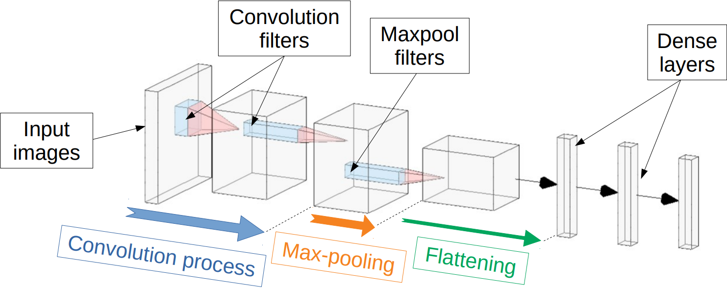
Figure 1: Image convolutional processing inside a CNN. Image generated with [44].

The CNN regression task on complex input data such as images is intrinsically difficult. The training of deep representations of features combined with the training of a dense network on a large flatten feature representation are required. Sometimes, the image information is also spread across several input channels as we will see later when dealing with I and Q GNSS correlation images (see section 3). Therefore, the regression model has to construct complex features representations from the various channels, adding even more complexity to the overall regression process. In order to ease the training of such multi-channel regression, in the next section, we will propose to use a soft label procedure. The main idea is to learn soft labels rather than sharp target continuous values.

Note that in the following, the response of the complete neural network regression model will be written as $y=N_{\theta}(x)$ where $\theta=(\lambda,W)$ and $\lambda$ represent filter and connection weights from the CNN network architecture up to the penultimate dense layer and $W$ is the weight matrix storing all connection weights from the last dense layers.

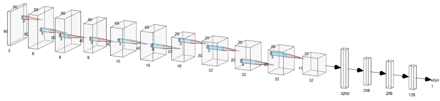
Figure 2: CNN architecture used for regression task on 80x80 images. Image generated on [44].

2.2 Soft labelling using distributional loss

In this section, we recall the concept of distributional loss as proposed in [1]. Traditionally, given an input $x$, the regression task consists in computing the parameter $\theta$ of a regression model $N_{\theta}$ that would assign predicted values $N_{\theta}(x)$ for given inputs $x$ and targets $y$. The target values $y$ can be seen as expected values of an underlying distribution of $Y|x$ assumed to be Gaussian. Therefore, in this setting, it is natural to calibrate the parameter $\theta$ by minimizing a square loss function $(N_{\theta}(x)-y)^{2}$.
The target value $y$ is usually considered as the ground truth and obtained by experiments or measurements. However, it may be subject to uncertainty or ambiguity [11] and may impair the generalization performance of the regression model. The main idea of soft labelling is to consider that the target value is an observation of an underlying ground truth distribution and one may benefit from learning the distribution rather than the individual targets.
To do so, consider now the task of learning the distribution $Y|x$ instead of predicting directly $\mathbb{E}[Y|x]$. For each target value, a target distribution $Y|x$ is chosen. This choice is of course problem dependent. However in [1], it has been shown experimentally, when no prior knowledge on the target distribution is known, that the use of a truncated Gaussian is the best choice among a variety of other distributions. In the sequel of the article, we will therefore assume that $Y|x\sim\mathcal{N}_{[a,b]}(\mu,\sigma^{2})$ where $\mathcal{N}_{[a,b]}(\mu,\sigma^{2})$ is the truncated Gaussian distribution of mean $\mu$ and variance $\sigma^{2}$ on the interval $[a,b]$ with density

$$f_{\mu,\sigma,[a,b]}(y)=\frac{1}{\sigma}\frac{\varphi(\frac{y-\mu}{\sigma})}{\phi(\frac{b-\mu}{\sigma})-\phi(\frac{a-\mu}{\sigma})}\mathds{1}_{[a,b]}(y)$$

where $\varphi$ and $\phi$ are the density and the cumulative distribution functions of the standard normal distribution $\mathcal{N}(0,1)$.
In order to learn the target distributions, a discrete version of $Y|x$ is considered in the form of an histogram with $K$ bins. During training, as we are now comparing the estimated distribution $N_{\theta}(x)$ and the target distribution $f_{\mu,\sigma,[a,b]}$, we can use the KL divergence as a loss function. It is defined as follows

$$\mathcal{D}_{\mathit{KL}}(p||q)=\int_{-\infty}^{+\infty}p(y)\log\frac{p(y)}{q(y)}dy$$

and measures how different $q$ is from $p$. Using $\mathcal{D}_{\mathit{KL}}$ as a loss function will require to minimize simply the following term also known as the cross-entropy

$$h(p,q)=-\int_{-\infty}^{+\infty}p(y)\log q(y)dy.$$

If $q$ is the estimated density and $p$ is the target distribution with density $f_{\mu,\sigma,[a,b]}$, the cross-entropy can be written as

$$h(f_{\mu,\sigma,[a,b]},q)=-\int_{a}^{b}f_{\mu,\sigma,[a,b]}(y)\log q(y)dy.$$

For each input $x$, the estimated discrete distribution $q$ is a $K$-dimensional vector where each component $i$ returns a probability $q_{i}=(N_{\theta}(x))_{i}$ that the target value is in the bin $i$. The number of bins $K$ will be an hyper-parameter of the method. The discrete target distribution $p$ corresponding to $f_{\mu,\sigma,[a,b]}$ can also be seen as a $K$-dimensional vector where each component $i$ returns the probability mass $p_{i}=F(a_{i}+t_{i})-F(a_{i})$ contained in the $i$-th bin, where $a_{i}$ and $t_{i}$ are the left bound and the width of the bin respectively and $F$ is the cumulative distribution of $f_{\mu,\sigma,[a,b]}$. Therefore, for a given input $x$ the distributional Histogram Loss (HL) can be written as follows

$$\mathit{HL}(x)=-\displaystyle\sum_{i=1}^{K}p_{i}\log(N_{\theta}(x))_{i}$$

$$\mathit{HL}(x)=-\sum_{i=1}^{K}\left[F(a_{i}+t_{i})-F(a_{i})\right]\log(N_{\theta}(x))_{i}$$

After training, for a given input $x$, $\mathbb{E}[N_{\theta}(x)]$ will provide the estimated value of $\mathbb{E}[Y|x]$. In [1, 11], experiments have shown that learning target distributions rather than hard target values will improve the generalization power of the model. This method is different from transforming the regression task into a classification task by discretizing uniformly the support set of target values. Here, a target distribution is assumed and learned during the process. Additionally, by tuning the variance parameter $\sigma$ and the number of bins used to transform the target distribution into an histogram, it is possible to adjust the bias-variance trade-off achieved by the model.

2.3 Dedicated CNN architectures

In this study, in order to compare the HL strategy with the classical CNN-Regression (CNN-Reg), two VGG-like architectures [43] will be used. Sharing the same backbone as shown in Figure 2, they only differ in their outputs. The extraction part is composed by 3 convolution blocks, each formed by consecutive convolutional layers and ended by a max-pooling layer. The number of filters is increasing with the depth of the convolutional layers. At the end of the convolutional process, the data are flattened to feed the 3 hidden dense layers. The output layer consists in a single neuron equipped with a linear activation function for the baseline CNN-Reg, and a softmax layer with $K$ outputs in the soft labelling case. To differentiate the two algorithms, we will refer to the network with a single output as CNN-Reg and the one using the softmax output as CNN-Histogram Loss (CNN-HL).

3 Application to GNSS multi-path parameter estimation

3.1 Problem statement

The GNSS positioning principle is based on the distance measurement between satellites of known positions and the receiver to locate. Using the propagation time of a dedicated signal emitted by the satellite, the receiver estimates its relative distance to the satellite [45]. Using several distances, the receiver is able to calculate its position by trilateration.

More precisely, the calculation process of the Position Time Velocity (PVT) solution relies on the synchronisation between the received signal and a receiver replica of the wanted signal. The alignment between both signals requires the estimation of the three unknown parameters of the incoming signal which are:

• The propagation delay $\tau$,

• The Doppler shift frequency $f_{\mathit{D}}$,

• The carrier phase $\phi$.

In a classical receiver, this estimation process is typically conducted by mean of the maximum likelihood principle. It is implemented through the maximization of the cross-correlation between the received signal and a local replica signal parameterized by three test values $\tilde{\tau}$, $\tilde{f_{D}}$ and $\tilde{\phi}$. In practice, the correlation operation is accomplished through a product followed by an integrate and dump stage. To be complete, it should also be pointed out that correlation is split into two orthogonal channels, named by convention In-phase (I) and in-Quadrature (Q). The maximization task is generally carried out by loop systems, namely the Delay-Locked Loop (DLL) and the Phase-Locked Loop (PLL). In addition, the loops present the intrinsic advantage to track the target parameters which are time-varying due to the continuously changing receiver-satellites geometry. No more than three correlation points per I and Q channels are usually required for normal loop operation.

However, various kinds of interference can deteriorate the positioning process. Multi-path is one of the most common and the most harmful interference. A multi-path is a reflection on a surrounding obstacle of the useful signal picked up by the receiving antenna concurrently to the Line-Of-Sight (LOS) signal. An illustration of the phenomenon is shown in Figure 3, generated by the SE-Nav software [46], a signal propagation simulator. In general, a receiver is impacted by multiple multi-paths, especially in urban environments where reflectors are numerous. Sometimes, the direct path may even be absent due to an obstruction, for example when high buildings are surrounding the receiver [47]. However, in this study the assumption is made that the direct path is always present and a single multi-path will be considered. Being the replica of the signal of interest, the multi-path contains the same information but with shifted parameters:

• The code delay in excess compared with the useful signal $\Delta\tau_{\mathit{MP}}$,

• The difference in Doppler shift frequency with the useful signal $\Delta f_{\mathit{MP}}$,

• The phase difference with the useful signal $\Delta\phi_{\mathit{MP}}$,

• The attenuation of the multi-path with respect to the magnitude of the useful signal $\alpha_{\mathit{MP}}$.

The addition of the multi-path to the direct signal biases the result of the correlation operation. As a consequence, the estimation of the incoming signal parameters is altered and the accuracy of the position delivered to the user may be degraded. With as few as three correlation points per channel, the information available to detect the multi-path contamination and possibly mitigate its effects is poor.

This work proposes to use a larger number of correlation points in order to overcome this lack of information. Indeed, $\tilde{\tau}$ and $\tilde{f_{\mathit{D}}}$ each sample a specific range, forming a 2-D grid. The correlation outputs in turn compose a 2-D matrix, in other words an image. The signal having 2 channels, I and Q, there will be two 2D-images at the output of the correlators. The general process is depicted in Figure 6. Figures 1 and 5 are given as detailed examples of the resulting images. Concerning the estimation of $\phi$, the necessary information is available through the orthogonality property of the I and Q channels, the first one granting access to $\cos(\phi)$ and the second to $\sin(\phi)$. The image construction is detailed in [38].

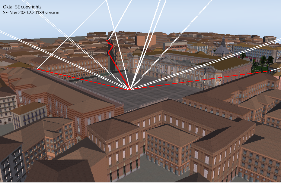
Figure 3: GNSS receiver collecting LOS and NLOS signals in Toulouse city center (France).

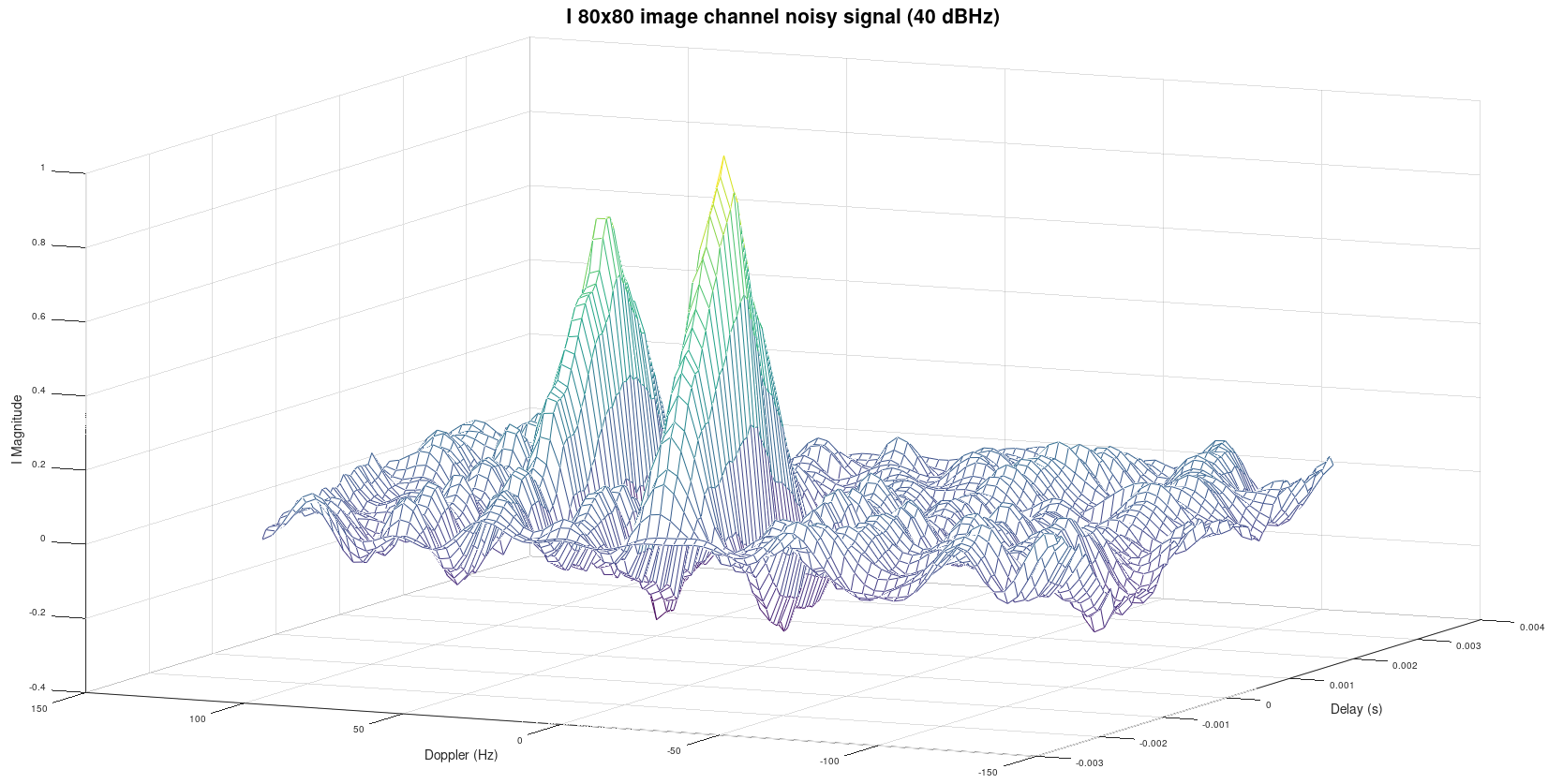
Figure 4: I channel for a signal undergoing a multi-path with $\tau_{\mathit{MP}}=0.75$ Tc , $f_{\mathit{MP}}=100$ $\mathrm{Hz}$, $\alpha_{\mathit{MP}}=0.8$, $\phi_{\mathit{MP}}=45^{\circ}$.

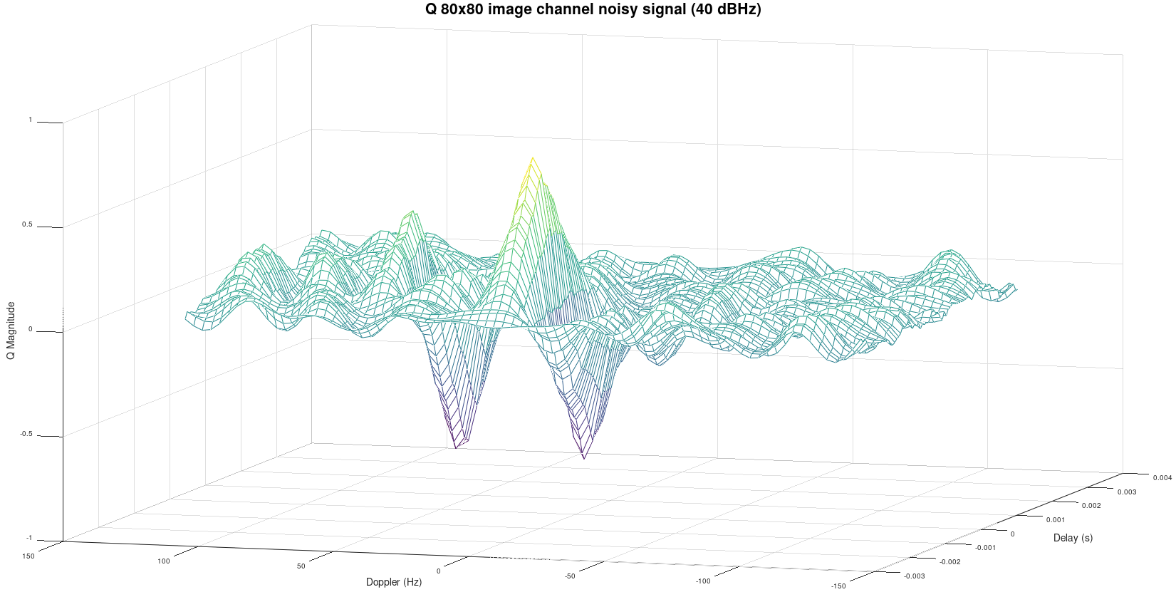
Figure 5: Q channel for a signal undergoing a multi-path with $\tau_{\mathit{MP}}=0.75$ Tc, $f_{\mathit{MP}}=100$ $\mathrm{Hz}$, $\alpha_{\mathit{MP}}=0.8$, $\phi_{\mathit{MP}}=45^{\circ}$.

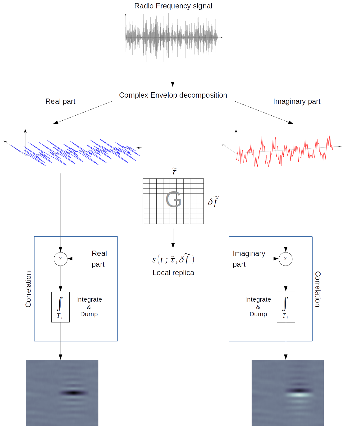
Figure 6: Illustration of the image elaboration process. The received signal is split in two orthogonal components. Next, each component is correlated with a local replica signal whose parameters span a grid G. The result forms a 2D-image. The pair of images then supplies the CNN implementing the regression task. The tilde notation indicates the local parameter by opposition to the received signal unknown parameter.

3.2 Experimental setup

3.2.1 Dataset definition

Experiments were made on several datasets which are divided into 2 groups. The first group is characterized by a fixed Carrier to Noise $\mathit{C\!/\!N0}$ ratio while the second has distinct $\mathit{C\!/\!N0}$ ratio levels. The $\mathit{C\!/\!N0}$ figure represents the ratio between the power of the signal of interest and the receiver intrinsic noise level. In the GNSS community it is considered as one of the most important figure of merit for the quality of the received signal. The higher the ratio, the more accurate the downstream parameter estimation.

In the first group, $\mathit{C\!/\!N0}$ is equal to 40 $\mathrm{d}\mathrm{B}\mathrm{Hz}$ to simulate a typical urban environment receiving condition. The multi-path attenuation $\alpha_{\mathit{MP}}$ is categorized to assess the performance of both CNN algorithms as a function of this parameter. In this way, we have:

• Strong multi-paths where $\alpha_{\mathit{MP}}\sim\mathcal{U}([0.6,0.9])$

• Moderated multi-paths where $\alpha_{\mathit{MP}}\sim\mathcal{U}([0.4,0.6])$

• Weak multi-paths where $\alpha_{\mathit{MP}}\sim\mathcal{U}([0.1,0.4])$

The second group is composed by datasets with different $\mathit{C\!/\!N0}$ ratio while $\alpha_{\mathit{MP}}\sim\mathcal{U}([0.1,0.9])$. The goal is to evaluate the algorithms with respect to $\mathit{C\!/\!N0}$, which takes the following values: 43 $\mathrm{d}\mathrm{B}\mathrm{Hz}$, 40 $\mathrm{d}\mathrm{B}\mathrm{Hz}$, 37 $\mathrm{d}\mathrm{B}\mathrm{Hz}$ and 34 $\mathrm{d}\mathrm{B}\mathrm{Hz}$.

Otherwise, all datasets share the same following variables:

• $\Delta\tau_{\mathit{MP}}$ is uniformly generated in $[0,1.5]$ Tc,

• $\Delta f_{\mathit{MP}}$ follows a truncated centered Gaussian distribution with standard deviation $\sigma=125/3$ $\mathrm{Hz}$. $\Delta f_{\mathit{MP}}$ is restricted to $[-3\sigma,+3\sigma]$ $\mathrm{Hz}$,

• $\Delta\phi_{\mathit{MP}}$ is uniformly generated in $[0,2\pi]$ .

Each dataset contains $10000$ samples, a sample being the I and Q image pair. In a dataset, image size does not change. However, to observe the CNN parameter estimation performance under lower input image resolutions, various datasets were created: 80x80, 40x40, 20x20 and 10x10 pixels images.

A synthetic correlator output generator [48] has been used to populate the datasets used in this study. The underlying signal model and the generation process are completely described in [38]. The generator is fully configurable with respect to the multi-path parameters $\mathit{C\!/\!N0}$, $\alpha_{\mathit{MP}}$, $\Delta\tau_{\mathit{MP}}$, $\Delta f_{\mathit{MP}}$ and $\Delta\phi_{\mathit{MP}}$. The resolution of the I & Q output images can also be set on demand.

3.2.2 Hyper-parameter selection

Performance results provided in the next section are results averaged over 10 runs. For each run, the training set is formed by randomly selecting $8000$ samples and the validation set by selecting randomly $1000$ samples among the $2000$ remaining samples. The last $1000$ samples constitute the test set.

CNN-Reg and CNN-HL were trained for 100 epochs and have used a $1000$ samples batch size. Learning rates of both CNN were empirically fixed to $10^{-3}$ and 3x3 filters were used for convolutional layers as shown in Figure 2. The number of bins for CNN-HL is fixed to $K=100$ (such as in [1]). The hyper-parameter $\sigma$ follows the following rule: $\sigma=2(b-a)/K$.

3.3 Results

Performance assessment is based on Mean Absolute Error (MAE) results averaged over 10 runs. For the CNN-Reg, the MAE metric is as follows:

$$\frac{1}{L}\sum_{l=1}^{L}|N_{\theta}(x_{l})-y_{l}|$$

where:

• $L$ is the number of samples in the test dataset,

• $x_{l}$ is the $l$-th test sample,

• $y_{l}$ is the target value for the $l$-th sample.

For the CNN-HL, the MAE metric is calculated as follows:

$$\frac{1}{L}\sum_{l=1}^{L}\left|\tilde{\mathbb{E}}[N_{\theta}(x)]-y_{l}\right|$$

with

$$\tilde{\mathbb{E}}[N_{\theta}(x)]=\sum_{i=1}^{K}q_{i,x_{l}}.c_{i}$$

and

• $q_{i,x_{l}}$ is the probability of the $i$-th softmax output neuron associated to $x_{l}$,

• $c_{i}$ is the center of the $i$-th bin for $i\in[1,K]$ (where the interval $[a,b]$ has been partitioned into $K$ equal subdivisions).

Tables 3.4, 3.4, 3.4 and 3.4 gather the averaged MAE performance results as defined above for the two algorithms CNN-Reg and CNN-HL on the first group of datasets.

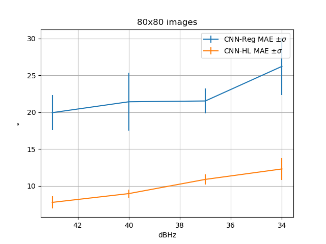
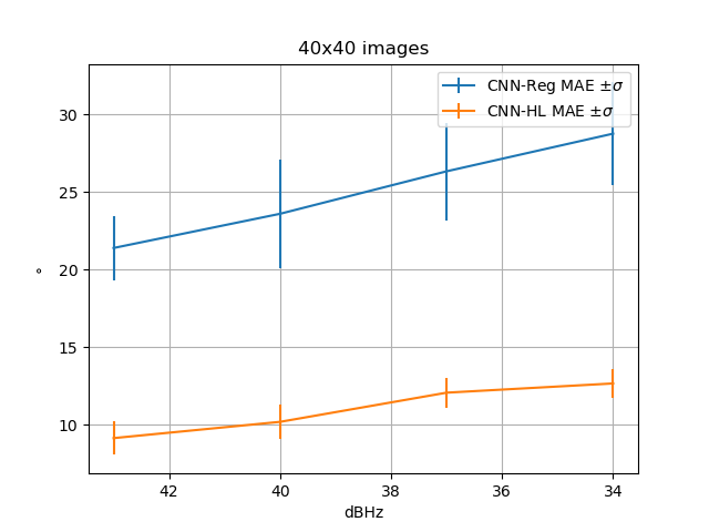
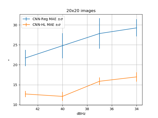
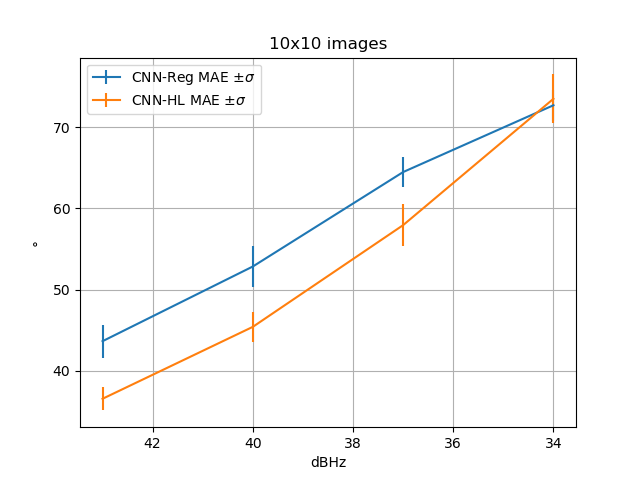
Figure 12: MAE behaviour according to $\mathit{C\!/\!N0}$ ratio for $\phi_{\mathit{MP}}$ estimation.

Figures 7, 8, 11 and 12, established with the second group of datasets, illustrate the CNN-Reg and CNN-Reg MAE behaviour when $\mathit{C\!/\!N0}$ varies. The curves are plotted according to a decreasing $\mathit{C\!/\!N0}$ because a high $\mathit{C\!/\!N0}$ corresponds to better receiving conditions. The scale on the x-axis starts from 43 $\mathrm{d}\mathrm{B}\mathrm{Hz}$ (good receiving conditions) and goes down to 34 $\mathrm{d}\mathrm{B}\mathrm{Hz}$ (deteriorated receiving conditions).

3.4 Results discussion

In Table 3.4, it can be observed that in all conditions and datasets, CNN-HL always shows better results than CNN-Reg. The delay $\tau_{\mathit{MP}}$ estimation performance is higher with CNN-HL on 20x20 images than the performance of CNN-Reg on 80x80 images. Additionally, as expected the average MAE and its standard deviation increase as the image resolution diminishes. In Table 3.4, similar results are observed for strong multi-paths. For moderate and weak multi-paths, the Doppler frequency estimation performance remains better on 40x40 images with CNN-HL than the performance of CNN-Reg on 80x80 images. In Tables 3.4 and 3.4, similar behaviour as $\tau_{\mathit{MP}}$ estimation are found. It can be noticed that in the particular case of $\alpha_{\mathit{MP}}$ estimation, the average MAE decreases as the strength of the multi-path decreases. This could be explained by the fact that in strong, moderate and weak multi-path datasets, the $\alpha_{\mathit{MP}}$ parameter estimation is biased by the dataset design that only contains ranges of $\alpha_{\mathit{MP}}$ parameters. In Table 3.4, $\phi_{\mathit{MP}}$ estimation with both CNN shows difficulties. For weak multi-paths on 40x40 images, the average MAE remains at a level of $14^{\circ}$ which might not be sufficient for practical multi-path mitigation use.

Average MAE $\tau_{\mathit{MP}}$ estimation error in $10^{-2}$ Tc for different multi-path attenuations. Dataset Image size Algorithm CNN-Reg CNN-HL Strong multi-paths 80x80 2.50 $\pm$ 0.22 0.64 $\pm$ 0.18 40x40 2.91 $\pm$ 0.32 0.76 $\pm$ 0.11 20x20 4.30 $\pm$ 0.42 1.28 $\pm$ 0.20 10x10 6.70 $\pm$ 0.40 4.85 $\pm$ 0.17 Moderate multi-paths 80x80 3.03 $\pm$ 0.54 0.66 $\pm$ 0.04 40x40 3.44 $\pm$ 0.65 0.96 $\pm$ 0.26 20x20 4.44 $\pm$ 0.45 1.63 $\pm$ 0.15 10x10 9.90 $\pm$ 0.72 7.35 $\pm$ 0.38 Weak multi-paths 80x80 4.64 $\pm$ 1.44 1.01 $\pm$ 0.13 40x40 4.33 $\pm$ 0.42 1.55 $\pm$ 0.20 20x20 7.20 $\pm$ 1.55 2.86 $\pm$ 0.40 10x10 26.13 $\pm$ 1.96 21.17 $\pm$ 0.58

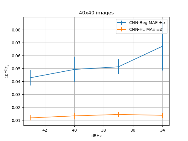
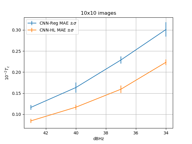
Figure 7: MAE behaviour according to $\mathit{C\!/\!N0}$ ratio for $\tau_{\mathit{MP}}$ estimation.

Average MAE $f_{\mathit{MP}}$ estimation error in $\mathrm{Hz}$ for different multi-path attenuations. Dataset Image size Algorithm CNN-Reg CNN-HL Strong multi-paths 80x80 1.22 $\pm$ 0.20 0.60 $\pm$ 0.04 40x40 1.60 $\pm$ 0.27 0.75 $\pm$ 0.07 20x20 2.36 $\pm$ 0.41 1.17 $\pm$ 0.12 10x10 5.16 $\pm$ 0.26 3.60 $\pm$ 0.18 Moderate multi-paths 80x80 1.33 $\pm$ 0.29 0.72 $\pm$ 0.06 40x40 1.70 $\pm$ 0.23 0.87 $\pm$ 0.06 20x20 2.61 $\pm$ 0.45 1.52 $\pm$ 0.11 10x10 7.08 $\pm$ 0.36 5.52 $\pm$ 0.27 Weak multi-paths 80x80 1.75 $\pm$ 0.31 1.26 $\pm$ 0.15 40x40 2.41 $\pm$ 0.38 1.42 $\pm$ 0.13 20x20 4.30 $\pm$ 0.41 2.84 $\pm$ 0.45 10x10 21.48 $\pm$ .68 19.04 $\pm$ 1.07

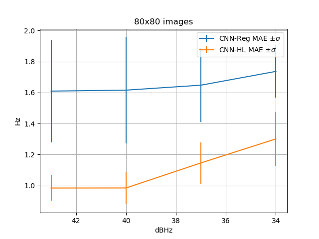
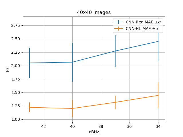
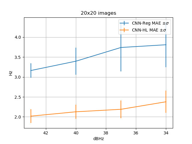
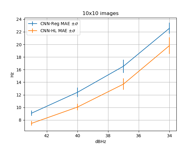
Figure 8: MAE behaviour according to $\mathit{C\!/\!N0}$ ratio for $f_{\mathit{MP}}$ estimation.

In Figures 9 and 10, a comparison of label and prediction distribution probabilities are shown. They correspond to a correct and a wrong estimation respectively. Each point of the plots represents the output of one of the $K$ neurons from the CNN-HL softmax layer. It can be noticed that in Figure 9, both curves are nearly superposed and both form a near Gaussian distribution. In the opposite, in Figure 10, the target and predicted probability distribution do not coincide. This situation corresponds to a wrong estimation. In this case, the Gaussian behaviour is not so well reconstructed.

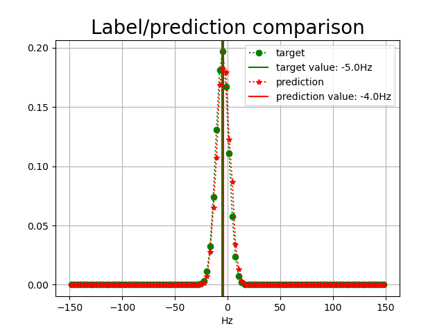
Figure 9: Comparison between the target and the prediction distribution probabilities for a correct prediction.

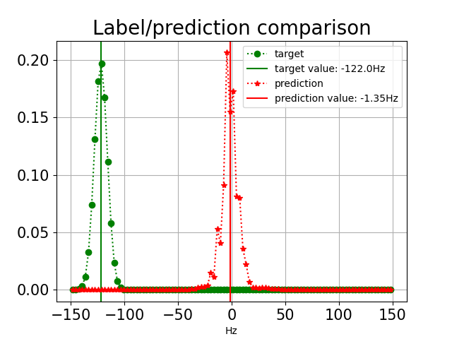
Figure 10: Comparison between the target and the prediction distribution probabilities for a wrong prediction.

$\alpha_{\mathit{MP}}$ estimation error in % for different multi-path attenuations. Dataset Image size Algorithm CNN-Reg CNN-HL Strong multi-paths 80x80 3.95 $\pm$ 0.93 1.30 $\pm$ 0.26 40x40 4.45 $\pm$ 0.61 1.48 $\pm$ 0.14 20x20 5.60 $\pm$ 0.70 2.22 $\pm$ 0.20 10x10 7.32 $\pm$ 0.40 5.99 $\pm$ 0.25 Moderate multi-paths 80x80 3.71 $\pm$ 0.64 1.08 $\pm$ 0.05 40x40 3.76 $\pm$ 0.53 1.22 $\pm$ 0.15 20x20 4.79 $\pm$ 0.55 1.73 $\pm$ 0.10 10x10 5.97 $\pm$ 0.16 5.00 $\pm$ 0.07 Weak multi-paths 80x80 3.53 $\pm$ 0.88 1.91 $\pm$ 1.16 40x40 4.06 $\pm$ 1.28 1.38 $\pm$ 0.57 20x20 4.09 $\pm$ 1.10 1.66 $\pm$ 0.22 10x10 7.87 $\pm$ 0.33 6.08 $\pm$ 0.12

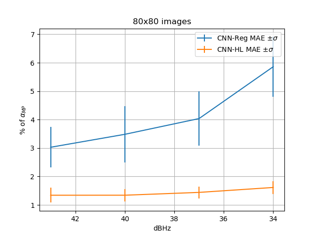
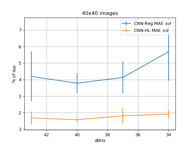
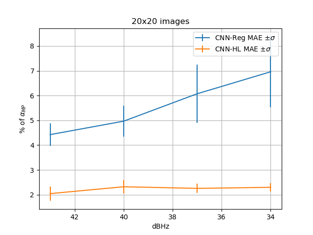
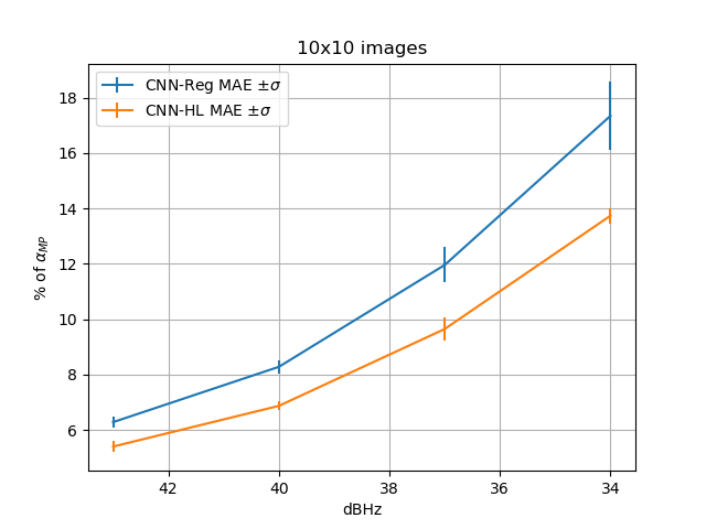
Figure 11: MAE behaviour according to $\mathit{C\!/\!N0}$ ratio for $\alpha_{\mathit{MP}}$ estimation.

$\phi_{\mathit{MP}}$ estimation error in degrees for different multi-path attenuations. Dataset Image size Algorithm CNN-Reg CNN-HL Strong multi-paths 80x80 12.30 $\pm$ 1.46 4.19 $\pm$ 0.81 40x40 15.41 $\pm$ 3.46 4.80 $\pm$ 0.67 20x20 15.59 $\pm$ 2.44 6.34 $\pm$ 0.69 10x10 29.68 $\pm$ 2.06 24.12 $\pm$ 1.11 Moderate multi-paths 80x80 15.71 $\pm$ 3.07 5.51 $\pm$ 0.89 40x40 15.72 $\pm$ 1.74 5.71 $\pm$ 0.88 20x20 17.90 $\pm$ 1.99 8.46 $\pm$ 1.03 10x10 42.55 $\pm$ 2.30 34.17 $\pm$ 2.02 Weak multi-paths 80x80 26.45 $\pm$ 6.25 10.23 $\pm$ 0.84 40x40 30.06 $\pm$ 3.35 14.12 $\pm$ 1.28 20x20 29.57 $\pm$ 3.17 17.15 $\pm$ 2.01 10x10 70.23 $\pm$ 1.56 68.82 $\pm$ 2.27

3.5 Results synthesis

The experiments made on the various datasets show the boosting effect of the CNN-HL algorithm which always performed better than CNN-Reg with not only a lower average MAE but also a lower standard deviation. The gain brought by the distributional technique allows more accurate and precise estimation on smaller images. The input size could be reduced from a resolution of 80x80 to 40x40 and sometimes 20x20. The results tend to indicate that the multi-path phase estimation is a more difficult task and the level of performance achieved by the models might not be sufficient in practice.

4 Conclusions

Estimating information from images is a useful but difficult task. In this work, we have addressed deep learning regression from multiple images channels. The proposed model makes use of convolutional neural layers in order to extract high level features from images. Instead of carrying out classical regression on these extracted features, a soft labelling approach is used to learn underlying target distributions. The idea is to allow the neural network model to account for some uncertainty in the target and therefore increase its generalization performance. The target distributions are modeled using histograms and a specific histogram loss function based on the KL divergence is applied during training. The resulting neural architecture incorporates a softmax output in order to reconstruct the histogram discrete target probability. The complete process could be applied to any applications that requires inference of function values from multiple images channels. The model is applied to GNSS multi-path estimation where multi-path signal parameters have to be estimated from correlator output images from the I and Q channels. The multi-path signal delay, attenuation, Doppler frequency and phase parameters are estimated from synthetically generated datasets of satellite signals. Experiments are conducted under various receiving conditions and various input images resolutions. For all receiving conditions that have been tested, the proposed soft labelling CNN technique using distributional loss outperforms classical CNN regression. In addition, the gain in accuracy obtained by the model allows downsizing of input image resolution from 80x80 down to 40x40 or sometimes 20x20. This reduction of image resolution is a first step towards the implementation of such models in physical receivers that are limited in the number of correlator outputs that can be designed. Despite real datasets are difficult to construct and label, further research using the CNN-HL model on GNSS data should focus on data that incorporates real receiving conditions. Additionally, from a model perspective, future investigation should propose adaptive histogram loss techniques that adjust the number of bins and target distribution parameters to the data.

References

- [1] E. Imani and M. White, “Improving regression performance with distributional losses,” in Proceedings of the 35th International Conference on Machine Learning, ser. Proceedings of Machine Learning Research, J. Dy and A. Krause, Eds., vol. 80. PMLR, 10–15 Jul 2018, pp. 2157–2166. [Online]. Available: https://proceedings.mlr.press/v80/imani18a.html
- [2] I. Goodfellow, Y. Bengio, and A. Courville, Deep Learning. MIT Press, 2016, http://www.deeplearningbook.org.
- [3] A. Toshev and C. Szegedy, “Deeppose: Human pose estimation via deep neural networks,” 2014 IEEE Conference on Computer Vision and Pattern Recognition, pp. 1653–1660, 2014.
- [4] S. Mahendran, H. Ali, and R. Vidal, “3d pose regression using convolutional neural networks,” 2017 IEEE International Conference on Computer Vision Workshops (ICCVW), pp. 2174–2182, 2017.
- [5] S. Li and A. B. Chan, “3d human pose estimation from monocular images with deep convolutional neural network,” in ACCV, 2014.
- [6] R. B. Girshick, J. Shotton, P. Kohli, A. Criminisi, and A. W. Fitzgibbon, “Efficient regression of general-activity human poses from depth images,” 2011 International Conference on Computer Vision, pp. 415–422, 2011.
- [7] D. Yi, Z. Lei, and S. Li, “Age estimation by multi-scale convolutional network,” in ACCV, 2014.
- [8] M. Ueda, K. Ito, K. Wu, K. Sato, Y. Taki, H. Fukuda, and T. Aoki, “An age estimation method using 3d-cnn from brain mri images,” 2019 IEEE 16th International Symposium on Biomedical Imaging (ISBI 2019), pp. 380–383, 2019.
- [9] S. Miao, Z. J. Wang, and R. Liao, “A cnn regression approach for real-time 2d/3d registration,” IEEE Transactions on Medical Imaging, vol. 35, pp. 1352–1363, 2016.
- [10] S. Lathuilière, P. Mesejo, X. Alameda-Pineda, and R. Horaud, “A comprehensive analysis of deep regression,” IEEE Transactions on Pattern Analysis and Machine Intelligence, vol. 42, no. 9, pp. 2065–2081, 2020.
- [11] B.-B. Gao, C. Xing, C.-W. Xie, J. Wu, and X. Geng, “Deep label distribution learning with label ambiguity,” IEEE Transactions on Image Processing, vol. 26, no. 6, p. 2825–2838, Jun 2017. [Online]. Available: http://dx.doi.org/10.1109/TIP.2017.2689998
- [12] S. Ioffe and C. Szegedy, “Batch normalization: Accelerating deep network training by reducing internal covariate shift,” in Proceedings of the 32nd International Conference on International Conference on Machine Learning - Volume 37, ser. ICML’15. JMLR.org, 2015, p. 448–456.
- [13] G. E. Hinton, N. Srivastava, A. Krizhevsky, I. Sutskever, and R. R. Salakhutdinov, “Improving neural networks by preventing co-adaptation of feature detectors,” CoRR, vol. abs/1207.0580, 2012, cite arxiv:1207.0580. [Online]. Available: http://arxiv.org/abs/1207.0580
- [14] T. Zhang and B. Yu, “Boosting with early stopping: Convergence and consistency,” The Annals of Statistics, vol. 33, no. 4, pp. 1538–1579, 2005. [Online]. Available: http://www.jstor.org/stable/3448617
- [15] N. P. Couellan, “Probabilistic robustness estimates for feed-forward neural networks,” Neural networks, vol. 142, pp. 138–147, 2021.
- [16] ——, “The coupling effect of lipschitz regularization in neural networks,” SN Comput. Sci., vol. 2, p. 113, 2021.
- [17] T. Kos, I. Markezic, and J. Pokrajcic, “Effects of multipath reception on gps positioning performance,” in Proceedings ELMAR-2010, Sep. 2010, pp. 399–402.
- [18] A. J. Van Dierendonck, P. Fenton, and T. Ford, “Theory and performance of narrow correlator spacing in a GPS receiver,” Navigation, vol. 39, no. 3, pp. 265–283, 1992. [Online]. Available: https://onlinelibrary.wiley.com/doi/abs/10.1002/j.2161-4296.1992.tb02276.x
- [19] B. Townsend and P. Fenton, “A practical approach to the reduction of pseudorange multipath errors in a Ll GPS receiver,” in Proceedings of the 7th International Technical Meeting of the Satellite Division of The Institute of Navigation (ION GPS 1994), 1994, pp. 143–148.
- [20] L. Garin and J.-M. Rousseau, “Enhanced strobe correlator multipath rejection for code & carrier,” in Proceedings of the 10th International Technical Meeting of the Satellite Division of The Institute of Navigation (ION GPS 1997), September 1997, pp. 559–568.
- [21] G. A. McGraw and M. S. Braasch, “GNSS multipath mitigation using gated and high resolution correlator concepts,” in Proceedings of the 1999 National Technical Meeting of The Institute of Navigation, 1999, pp. 333–342.
- [22] N. Jardak, A. Vervisch-Picois, and N. Samama, “Multipath insensitive delay lock loop in GNSS receivers,” IEEE Transactions on Aerospace and Electronic Systems, vol. 47, no. 4, pp. 2590–2609, OCTOBER 2011.
- [23] B. Townsend, R. Van Nee, P. Fenton, and K. Van Dierendonck, “Performance evaluation of the multipath estimating delay lock loop,” in Proceedings of the 1995 National Technical Meeting of The Institute of Navigation, 1995, pp. 277–283.
- [24] M. Sahmoudi and M. G. Amin, “Fast iterative maximum-likelihood algorithm (fimla) for multipath mitigation in the next generation of gnss receivers,” IEEE Transactions on Wireless Communications, vol. 7, no. 11, pp. 4362–4374, November 2008.
- [25] N. Blanco-Delgado and F. D. Nunes, “Multipath estimation in multicorrelator gnss receivers using the maximum likelihood principle,” IEEE Transactions on Aerospace and Electronic Systems, vol. 48, no. 4, pp. 3222–3233, October 2012.
- [26] H. Qin, X. Xue, and Q. Yang, “Gnss multipath estimation and mitigation based on particle filter,” IET Radar, Sonar & Navigation, vol. 13, no. 9, pp. 1588–1596, 2019. [Online]. Available: https://ietresearch.onlinelibrary.wiley.com/doi/abs/10.1049/iet-rsn.2018.5587
- [27] Y. Zhang and C. Bartone, “Multipath mitigation in the frequency domain,” in PLANS 2004. Position Location and Navigation Symposium (IEEE Cat. No.04CH37556), 2004, pp. 486–495.
- [28] ——, “Real-time multipath mitigation with wavesmoothtm technique using wavelets,” in Proceedings of the 17th International Technical Meeting of the Satellite Division of The Institute of Navigation (ION GNSS 2004), 2004, pp. 1181–1194.
- [29] W. Vigneau, O. Nouvel, M. Manzano-Jurado, C. Sanz, A. H. Carrascosa, D. Roviras, J. M. Juan, and P. Holsters, “Neural networks algorithms prototyping to mitigate GNSS multipath for LEO positioning applications,” in Proceedings of the 19th International Technical Meeting of the Satellite Division of The Institute of Navigation (ION GNSS 2006), 2006, pp. 1752–1762.
- [30] H. Phan, S.-L. Tan, I. Mcloughlin, and L. Vu, “A unified framework for GPS code and carrier-phase multipath mitigation using support vector regression,” Advances in Artificial Neural Systems, 03 2013.
- [31] L. Hsu, “GNSS multipath detection using a machine learning approach,” in Proceedings of the 2017 IEEE 20th International Conference on Intelligent Transportation Systems (ITSC), Oct 2017, pp. 1–6.
- [32] T. Suzuki and Y. Amano, “NLOS multipath classification of GNSS signal correlation output using machine learning,” Sensors, vol. 21, no. 7, 2021. [Online]. Available: https://www.mdpi.com/1424-8220/21/7/2503
- [33] C. Savas and F. Dovis, “Multipath detection based on k-means clustering,” in Proceedings of the 32nd International Technical Meeting of the Satellite Division of The Institute of Navigation (ION GNSS+ 2019), 2019, pp. 3801–3811.
- [34] Y. Quan, L. Lau, G. Roberts, X. Meng, and C. Zhang, “Convolutional neural network based multipath detection method for static and kinematic GPS high precision positioning,” Remote Sensing, vol. 10, no. 12, 12 2018.
- [35] E. Schmidt, N. Gatsis, and D. Akopian, “A GPS spoofing detection and classification correlator-based technique using the LASSO,” IEEE Transactions on Aerospace and Electronic Systems, vol. 56, no. 6, pp. 4224–4237, Dec 2020.
- [36] Y. Tao, C. Liu, T. Chen, X. Zhao, C. Liu, H. Hu, T. Zhou, and H. Xin, “Real-time multipath mitigation in multi-gnss short baseline positioning via cnn-lstm method,” Mathematical Problems in Engineering, vol. 2021, p. 6573230, Jan. 2021. [Online]. Available: https://doi.org/10.1155/2021/6573230
- [37] S.-H. Kong, S. Cho, and E. Kim, “Gps first path detection network based on mlp-mixers,” IEEE Transactions on Wireless Communications, pp. 1–1, 2022.
- [38] A. Blais, N. Couellan, and E. Munin, “A novel image representation of gnss correlation for deep learning multipath detection,” Array, p. 100167, 2022. [Online]. Available: https://www.sciencedirect.com/science/article/pii/S2590005622000297
- [39] A. Siemuri, H. Kuusniemi, M. S. Elmusrati, P. Välisuo, and A. Shamsuzzoha, “Machine learning utilization in gnss—use cases, challenges and future applications,” in 2021 International Conference on Localization and GNSS (ICL-GNSS), June 2021, pp. 1–6.
- [40] T. Hastie, R. Tibshirani, and J. Friedman, The Elements of Statistical Learning, ser. Springer Series in Statistics. New York, NY, USA: Springer New York Inc., 2001.
- [41] K. P. Murphy, Machine Learning: A Probabilistic Perspective. The MIT Press, 2012.
- [42] Y. Lecun, L. Bottou, Y. Bengio, and P. Haffner, “Gradient-based learning applied to document recognition,” Proceedings of the IEEE, vol. 86, no. 11, pp. 2278–2324, 1998.
- [43] K. Simonyan and A. Zisserman, “Very deep convolutional networks for large-scale image recognition,” in 3rd International Conference on Learning Representations, ICLR 2015, San Diego, CA, USA, May 7-9, 2015, Conference Track Proceedings, Y. Bengio and Y. LeCun, Eds., 2015. [Online]. Available: http://arxiv.org/abs/1409.1556
- [44] A. LeNail, “NN-SVG: Alexnet.” [Online]. Available: https://alexlenail.me/NN-SVG/AlexNet.html
- [45] J. B.-Y. Tsui, Fundamentals of Global Positioning System Receivers: A Software Approach, 2nd ed., ser. Wiley Series in Microwave and Optical Engineering, K. Chang, Ed. Wiley-Blackwell, January 2005, iSBN-13: 978-0-471-70647-2.
- [46] Oktal-SE, “SE-Nav software,” firm specialized in electro-optical simulation, 31320 Vigoulet-Auzil, France. [Online]. Available: https://www.oktal-se.fr/
- [47] N. I. Ziedan, “Improved multipath and NLOS signals identification in urban environments,” NAVIGATION, vol. 65, no. 3, pp. 449–462, 2018. [Online]. Available: https://onlinelibrary.wiley.com/doi/abs/10.1002/navi.257
- [48] A. Blais, E. Munin, and N. Couellan, “A synthetic GNSS correlator output generator,” 2021. [Online]. Available: https://github.com/AntoineBlaisENAC/Synthetic_GNSS_Correlator_Output_Generator.git