Multi-Asset Bubbles Equilibrium Price Dynamics

Abstract

The price-bubble and crash formation process is theoretically investigated in a two-asset equilibrium model. Sufficient and necessary conditions are derived for the existence of average equilibrium price dynamics of different agent-based models, where agents are distinguished in terms of factor and investment trading strategies. In line with experimental results, we show that assets with a positive average dividend, i.e., with a strictly declining fundamental value, display at the equilibrium price the typical hump-shaped bubble observed in experimental asset markets. Moreover, a misvaluation effect is observed in the asset with a constant fundamental value, triggered by the other asset that displays the price bubble shape when a sharp price decline is exhibited at the end of the market.

Keywords: Bubbles, Agent-based models, Experimental economics, Equilibrium dynamics, Multi-asset market.
JEL codes: C62, C90, D40, G14.

1 Introduction

Financial bubbles cast doubt over agents’ rationality and represent possible sources of inefficiencies and market fragilities. However, due to the several underlying mechanisms that can lead to their formation, a clear understanding of the origins of the price bubble is still missing. Market restrictions are interestingly related to explaining the price bubble phenomena. Indeed, in a market where short-selling is not allowed, the price dynamics can be raised by “excessively optimistic” traders making the market generally overvalued, (Miller, , 1977). Moreover, market liquidity plays a relevant role to produce spillovers contagion effect, which leads to (flash) crashes events (CFTC-SEC, 2010, Cespa and Foucault, 2014, Kirilenko et al., 2017, da Gama Batista et al., 2017). On top of that, price bubbles can be attributed to agent’s confusion, lack of rationality, speculation and other factors, see e.g., Smith et al., (1988), Haruvy and Noussair, (2006), Kirchler et al., (2012), Baghestanian et al., (2015).

Since the seminal paper of Smith et al., (1988) (henceforth, SSW), experimental asset markets proved to be a powerful tool for analyzing bubble-crash patterns and the agents’ behavioural strategies through laboratory market experiments. Indeed, these price bubbles and crashes are robust and persistent under different experimental laboratory settings. For instance, Kirchler et al., (2012) explored where agents’ confusion about fundamental value combined with ample liquidity can lead to significant mispricing and overvaluation and so increasing the price bubble-shape pattern.

However, rational bubble theories, e.g., Blanchard, (1979), Tirole, (1985), Froot and Obstfeld, (1991), provide little help to properly understand laboratory asset bubble phenomena. This difficulty in linking existing price formation theories to laboratory asset markets emphasizes the puzzling feature of these experimental price bubbles, (Smith et al., , 2000). Thus, in the spirit of Duffy and Ünver, (2006), Haruvy and Noussair, (2006), Caginalp and Ilieva, (2008), and Baghestanian et al., (2015), we aim to theoretically investigate the price-bubble mechanism employing agent-based approaches, instead of conducting additional experiments.

In this work, sufficient and necessary conditions are presented for the existence of average equilibrium price dynamics of various agent-based models in a two-asset market. Specifically, one asset has a declining fundamental value, named speculative asset, while the other has a constant fundamental value, referred to as value asset. Starting from the single-asset Duffy and Ünver, (2006) (henceforth, DU) model, we show how to recover and analyze the price formation process finding the related equilibrium and average price dynamics expressions. We then extend the DU model to the two-asset case, presenting different factor trading strategies characterizing the equilibrium prices in the two assets market. Then, following Baghestanian et al., (2015), we introduce heterogeneous agents with (short-horizon) investment strategies, allowing us to relax the use of exogenous probability of the standard DU model to decide whether a trader is a buyer or a seller. For those assets with a positive average dividend, i.e., speculative assets, the typical price hump-shaped of price bubble observed in experimental asset markets is displayed at equilibrium price dynamics.

The DU model is one of the first model to employ an agent-based computational approach with noise (“near-zero-intelligence”) traders to study the sources of bubble-crash patterns in a single-asset market, replicating the experiments of SSW. Duffy and Ünver, (2006) have followed the methodology of Gode and Sunder, (1993, 1994) to explore the role of “zero-intelligence” machine traders in experimental markets, comparing the results from the artificial traders market with that of human traders.

In a trading round, the traders of the DU model have to decide two things: the position, i.e., they have to choose to be sellers or buyers, and the quote, i.e., the amount they are willing to sell/buy. The traders’ positions are decided in each trading round by a Bernoulli variable, where the probability of being a buyer decreases in each round, so that in the last trading sessions, traders are more prone to sell. This last condition is called weak-foresight assumption. Once decided the position, traders place orders following a weighted average between the previous period prices and a (random) value proportional to the fundamental value, which incorporates traders’ confusion about the fundamental value. The weighting parameter is called anchoring parameter, where a high value indicates that traders are more likely to post quotes close to the previous period prices. The anchoring effect captures the behavioural notion that anchoring might be relevant to explaining price-bubble shape, because it causes transaction prices to start low and subsequently rise as trade proceeds, see Duffy and Ünver, (2006) and Baghestanian et al., (2015).

Even though its simplicity, the DU model explains some of the underlying mechanisms of price bubbles through the agent-based model approach. For instance, when the fundamental value of the asset decreases over time, e.g., the average dividend of the asset is positive, agents start trading the stock at a low value compared to the fundamental one due to inexperience. Then, traders gain confidence to create an upward trend, with a subsequent soaring of the price dynamics. Agents will post quotes at a high level compared to fundamental values due also to their confusion about the fundamental value of the asset. This confusion is incorporated in the DU model by the underlying randomness of traders’ bid quotes. Then as the last trading rounds approach, large-scale selling orders are posted by traders since it decreases their subjectively perceived probability of being able to sell. This induced mechanism is modelled by DU employing the mentioned weak-foresight assumption.

On the other hand, the DU model setting contains some simplifications that make their model far from the real market setting and limit their results to the experimental context. For instance, the trading on one asset can trigger price changes on other assets, and, as seen during the Flash Crash of 2010, instability can influence a large set of assets, CFTC-SEC, (2010). The execution of asset portfolio orders, and more generally, the commonality in liquidity across assets, Chordia et al., (2000), Tsoukalas et al., (2019), may cause price changes among assets and due to cross-impact effects trigger significant instabilities effects across all market segments, Cordoni and Lillo, (2022). Therefore, in a multi-asset market, can the price bubble of one asset propagate to all the other assets? How would this propagation be characterized? Can spillover effects or specific (factorial) trading strategies, triggered by the bubble of one asset, also affect other assets’ price dynamics?

Interestingly, Caginalp et al., (2002) partially explored the above questions through experiments, where the presence of price-bubbles tends to increase volatility and diminishes prices of other stocks. Ackert et al., 2006a , Ackert et al., 2006b , have also investigated experiments with two assets, analyzing the effects of margin buying and short-selling where one of the asset is a lottery asset. Furthermore, Oechssler et al., (2007) performed experimental markets where five different assets can be traded simultaneously.

However, to the best of our knowledge, poor attention has been given to the study of multi-assets experimental markets employing agent-based modelling approaches to investigate the price-bubble mechanism. A recent further extension in a two-asset market of the DU model was proposed by Cordoni et al., (2022), where the role of market impact was investigated in the price bubble formation. In particular, each agent is designed in order to follow different factor-investing style strategies, where traders decide to buy or sell assets depending on the factor they have chosen. They found evidence that the liquidity mechanism which generates the price bubble does not involve a symmetric cross-impact (i.e., the price changes in one asset caused by the trading on other assets) between the two assets.

We present the different factor trading strategies characterizing the equilibrium prices on the two asset extension. When traders follow a factor trading strategy, the average price dynamics of the value asset will display a misvaluation. This difference between average prices and fundamental value of the value asset is triggered by the supply and demand imbalance generated by traders at the end of the market session when the speculative asset price-bubble declines. We investigate under which conditions this “contagion” effect of the price-bubble shape on the value asset, triggered by the sharp decline at the end of market periods, depending on the factor chosen by agents.

Another sticking point of the DU model is the use of an exogenous probability parameter by traders to decide whether to buy or sell an asset. Therefore, recently, their model has been generalized by Baghestanian et al., (2015) (in a single asset market), by introducing heterogeneous agents, which use fundamentalist and speculative (short-horizon) investment strategies together with noise traders. We combine the fundamentalists and speculators investment strategies with factor-investing style strategies, highlighting how an identification issue arises in the two-assets market equilibrium. Specifically, different market settings, which depend on the market factors chosen by agents, generate the same equilibrium price dynamics, confounding the origin and motivation of the average price-bubble dynamics. However, we identify the factor strategy characterizing the two-asset price equilibrium by extending the fundamentalist and speculative investment strategies to the two-assets case.

In Section 2 we introduce notation and our market setting. In Section 3 we recall the DU model and the corresponding equilibrium price is derived. In Section 4 and 5 we present our main results to the two-asset case using heterogeneous agent based model with factor and investment strategies, respectively. Finally, in Section 6 we conclude.

2 Market Setup

To investigate the price bubble and crash mechanism and the related price dynamics for a multi-assets market environment, we set up a market composed of two assets. The first asset has a positive average dividend $\overline{d}_{1}>0$, while the second asset average dividend is null, $\overline{d}_{2}=0$. Therefore, the two assets have different fundamental value dynamics; the fundamental value of the first asset, $FV_{1}$, decreases over time, while for the second one, $FV_{2}$, is constant. Unless specified, we follow the specifications presented in Duffy and Ünver, (2006) and Cordoni et al., (2022) by setting the dividend distribution support of asset $1$ equal to $\{\$0,\$0.1,\$0.16,\$0.22\}$ and terminal (buy-out) value $TV_{1}=\$1.80$, and for asset $2$, $\{\$-0.2,\$-0.1,\$0,\$0.1,\$0.2\}$ and terminal value $TV_{2}=\$2.80$, for asset 2, where a negative dividend corresponds to an holding cost, see Kirchler et al., (2012).

In the following, we investigate the existence of equilibrium price dynamics for the previous two-assets market. We first focus on a single-asset market composed only of the first asset and then generalize our results in the two-assets case.

3 The Duffy-Ünver Agent-Based model

The DU model involves $N$ agents who trade the same asset in $T$ trading periods. A random dividend is paid at the end of each trading period $t$. Then, the (average) fundamental value is given by

$$FV_{t,1}=(T-t+1)\overline{d}_{1}+TV_{1},$$

where $\overline{d}_{1}$ is the expected dividend payment, and $TV_{1}$ represents the terminal value. The dividends are drawn by a uniformly distributed random variable with finite support, while the terminal value is fixed to a constant value, (see Section 2). For the sake of simplicity, in this section, we omit the subscript $1$, since we focus only on the one-asset case.

In the original work of Duffy and Ünver, (2006) traders can post bid/ask quotes during submission rounds in trading time interval $t$. Precisely, each trading period $t$ is composed of $S$ submission rounds, where traders can place their orders following a double auction market mechanism with continuous open-order book dynamics. However, since we focus on the average equilibrium price, for our analysis we can omit this submission rounds architecture from the trading model.

At the beginning of market session, each trader $j$ has an endowment of cash $x^{j}$ and a quantity of the asset $y^{j}$. All agents are equally informed about the fundamental value dynamics. At trading period $t$ an agent $j$ is a buyer with probability $\pi_{t}$ and a seller with probability $1-\pi_{t}$, where it is assumed the so-called weak foresight assumptions, i.e., the probability of being a buyer is decreasing across the trading periods,

$$\pi_{t}=\max\{0.5-\varphi t,0\},\text{ where $\varphi\in\left[0,\frac{0.5}{T}\right)$. }$$

A positive $\varphi$ implies a gradual increase of excess supply towards the end of the market session and so it contributes to the reduction in mean transaction prices. This assumption makes the DU model results quite consistent with the experimental data of Smith et al., (1988), where also a decline in average transaction volume is observed across trading rounds. We discuss in detail the effect of this assumption in our equilibrium analysis. Each quote submitted by both a seller or a buyer is for one asset share. A buyer $j$ in period $t$ can place a bid quote if enough cash balances $x_{t}^{j}>0$ is available in his account. On the other hand, sellers can place an ask quote if they have enough share quantity, $y_{t}^{j}>0$. Thus, agent $j$ places a quote which is provided by a convex combination of the previous period mean traded price, $\overline{p}_{t-1}$, and a random quantity $u_{t}$. This random variable $u_{t}$ captures the uncertainty about agents’ decisions and it has a uniform distribution with support $[0,\kappa\cdot FV_{t}]$, where $\kappa>0$. If not specified, $\kappa$ is assumed to be greater than 1. This randomness was introduced by Duffy and Ünver, (2006) to capture agent’s confusion on the fundamental value.

At time $t=1$ Duffy and Ünver, (2006) set $\overline{p}_{0}=0$ in order to exactly replicate the same shape exhibited by SSW experiments. Specifically, this condition ensures that the price-bubble will start at a value below the fundamental value. This phenomenon in the SSW experiment results from the participants’ inexperience, and it induces an upward trend when agents gain confidence in adjusting the price to the fundamental value. Therefore, this condition artificially triggers the price-bubble mechanism, and we decide to set $\overline{p}_{0}$ equal to the fundamental value at time $t=1$, contrary to the DU model. Furthermore, the assumption of inexperienced participants is far from the real financial market, where traders are highly specialised due to the increase in market competitiveness. Therefore, our condition enables us to study the bubble mechanism in a complementary way with respect to Duffy and Ünver, (2006) analysis, since our zero-intelligence agents are assumed to be sufficiently more experienced than those of DU model. Moreover, this assumption is also in line with the recent experiments discussed in Baghestanian et al., (2015), where the price-bubble starts close to the fundamental value.

Therefore, if $j$ is a buyer, the trader will place a bid price, given by

$$b_{t}^{j}=\min\{(1-\alpha)u_{t}^{j}+\alpha\overline{p}_{t-1},x_{t}^{j}\},\quad\alpha\in(0,1)$$

where $u_{t}^{j}$ denotes the realization of the random variable $u_{t}$ for the $j$-th agent, and if $j$ is a seller, the agent will place, if $j$ has at least one share, an ask price given by

$$a_{t}^{j}=(1-\alpha)u_{t}^{j}+\alpha\overline{p}_{t-1}.$$

The parameter $\alpha\in(0,1)$ is called anchoring parameter and it represents agent’s attitude to post quotes close to previous period price. As observed by Duffy and Ünver, (2006) quotes converge on average to $\kappa\frac{FV_{t}}{2}$.

The anchoring parameter plays a crucial role in the price-bubble formation in the DU model. Prices will necessarily increase initially and decrease as the fundamental value decreases. Duffy and Ünver, (2006) argued that this kind of explanation for the price-bubble mechanism holds regardless of $\varphi$. However, when $\varphi=0$, the price will continue to get a “hump-shaped” path with no decrease in transaction volume. We completely characterize the equilibrium price dynamics in function of the above parameters in Section 3.1. The standard DU model agents are often referred to as near-zero-intelligence traders due to the simple trading strategies they implement and in the DU model extensions they are associated to noise traders strategies, see Baghestanian et al., (2015) and Cordoni et al., (2022).

3.1 Equilibrium Average Price Dynamics with Homogeneous Agents

Let us first introduce a first trivial result related to trader liquidity. Recall that $x_{t}^{j}$ is the cash endowment of trader $j$ at time $t$. All the proofs are reported in Appendix A.

Lemma 3.1.

There exists a finite amount of initial cash endowment, denoted as $x_{0}$, such that each trader can submit at least one buy order, at the bid price $q_{t}=(1-\alpha)u_{t}+\alpha\overline{p}_{t-1}$, during each trading period $t$ without going bankrupt, i.e., for each agent $j$, $x_{t}^{j}\geq 0$ for all $t$.

Thus, in the following we assume that:

Assumption 1.

Traders’ initial endowments are equal to $x_{0}^{j}=x_{0}$ and $y_{0}^{j}=1$ for each agent $j$, i.e., traders have enough endowment to at least submit one buy or sell quote for each trading time period $t$.

At first glance, the above assumption seems to limit the insights one can gain from the subsequent analysis. However, this assumption may be valid in a laboratory framework, where an experiment may be designed to guarantee that each participant can actively participate in the market. For instance, in the SSW experiment design, traders were provided with an endowment of cash and stock quantity equivalent to about $\$13$, which corresponds to have an initial endowment of $\$9.40$ and one stock. With this kind of endowment, we may expect that in the laboratory, no one of the agents will become bankrupt on average and can actively participate in the market, posting bids and asks quotes. This is what is also observed in the simulation analysis of Cordoni et al., (2022), where traders were equipped with an initial inventory of $\$10$ and two stocks and posted at least six outstanding orders for each trading period.

Remark 3.2.

We say the market is in equilibrium when the bid and ask prices are equal. Particularly, we are interested in studying the average equilibrium price dynamics, which can be recovered as the average of multiple laboratory sessions, i.e., by averaging the price dynamics resulting from different sessions. This implies that we are interested in the average behaviour of agents. Therefore, we may consider that a trader can be a buyer or a seller for a specific trading round and submit only one quote, representing the average quote without loss of generality. This design is similar to batch trading markets architecture and the average equilibrium price will be determined by simply equating the prevailing bid and ask price, where these prices will be obtained by equating the aggregate supply and demand for bid and ask sizes, respectively.

Thus, from Asm.1, for a trader $j$, $a_{t}^{j}=b_{t}^{j}=q_{t}$ for all $t.$ Hence, the prevailing bid price at time $t$, $p_{t}^{b}$, is the solution of

$$\sum_{j=1}^{N}\frac{\pi_{t}b_{t}^{j}}{p_{t}^{b}}=\sum_{j=1}^{N}\frac{\pi_{t}q_{t}}{p_{t}^{b}}=A_{t}$$

where $A_{t}$ is the supply provided by the market equal to $(1-\pi_{t})N$.

In the same way, the prevailing ask price at time $t$, $p_{t}^{a}$, is the solution of

$$\sum_{j=1}^{N}\frac{(1-\pi_{t})a_{t}^{j}}{p_{t}^{b}}=\sum_{j=1}^{N}\frac{(1-\pi_{t})q_{t}}{p_{t}^{a}}=B_{t}$$

where $B_{t}$ is the demand provided by the market, which is equal to $\pi_{t}N$.

On average an agent places an order equal to

$$\overline{q}_{t}=(1-\alpha)\kappa\frac{FV_{t}}{2}+\alpha\overline{p}_{t-1},$$

so that, on average,

$$p_{t}^{b}=\frac{\pi_{t}}{1-\pi_{t}}\overline{q}_{t};\quad p_{t}^{a}=\frac{1-\pi_{t}}{\pi_{t}}\overline{q}_{t}.$$

Definition 3.3.

The market-clearing price at equilibrium, $\overline{p}_{t}$, is defined as the price for which $p_{t}^{b}=p_{t}^{a}$, i.e., when the supply $A_{t}$ clear the demand $B_{t}$.

Remark 3.4.

The equilibrium price will be defined as the price such that bid and ask prices are equal. This notion is different from the standard concept of asset price equilibrium, which is that the asset price equals the present value of current and future payments. Perhaps, it would be better to replace the adjective equilibrium and use stationary price instead. However, the notion of stationary price might generate confusion in a price bubble dynamics framework. Therefore, we will continue to use the adjective of equilibrium, bearing in mind the conceptual difference with the standard notion of equilibrium.

Thus, as argued in Remark 3.2, we may analyse the average behaviour of agents. So, in the following analysis, for all agents, we consider the average bid/ask quote, i.e., we assume:

Assumption 2.

For each agent, we consider the average quote $q_{t}=\overline{q}_{t}$ for all $t.$

Essentially, we are examing the average submitted quotes for every agent, obtained by averaging across different market sessions according to the definition of agent’s behaviour of Duffy and Ünver, (2006). Specifically, traders can and will post different quotes for every market session, which can subsequently be aggregated to obtain the average quote $\overline{q}_{t}$.

Another way with which we might formulate the previous assumption, and reinterpret the model, is that the traders’ population can be divided into two representative agents, a buyer and a seller, which trade with the same average quote but with different volume, $(1-\pi_{t})N$ for the seller and $\pi_{t}N$ for the buyer. However, we remark that in this study we are not interested in trading volume predictions, contrary to the original work of Duffy and Ünver, (2006) and also to Baghestanian et al., (2015), and the following results can not be very insightful for that analyses, but instead, we focus on the price dynamics. On the other hand, we derive interesting insights about the order imbalance dynamics employed to describe a theoretical motivation of price bubbles in experiments. This will provide an additional perspective to the analysis carried out by Baghestanian et al., (2015) and it is outlined in Section 5.1.

Therefore, we may state our first results regarding the existence of the equilibrium market-clearing price.

Theorem 3.5.

Under assumptions 1, 2, the equilibrium market-clearing price $\overline{p}_{t}$ does not depend on the number of traders and it exists if and only if $\pi_{t}=\frac{1}{2}$. Moreover, $\overline{p}_{t}={q}_{t}$.

When $\pi_{t}\neq 0.5$ the market is not in equilibrium and there is an imbalance between demand and supply equal to $\left(\frac{B_{t}}{A_{t}}-1\right)$ which characterizes the average price dynamics:

$$p_{t}=q_{t}+\left(\frac{\pi_{t}}{1-\pi_{t}}-1\right).$$

For instance, when $\pi<0.5$, there are more sellers than buyers on average, so that the imbalance between demand and supply $\left(\frac{B_{t}}{A_{t}}-1\right)$ is negative. Therefore, the average price dynamics will result below the quote $q_{t}$, since the excess supply will push the price dynamics down. Interestingly, the price dynamics does not depend on the number of traders $N$. We then analyze the theoretical equilibrium price dynamics by varying the model parameters, $\kappa$, $\alpha$ and $\varphi$. To better quantify and visualize the misvaluation effect the Relative Deviation (RD) measure of Stöckl et al., (2010) is employed. RD satisfies all the evaluation criteria presented in Stöckl et al., (2010), i.e., (it relates fair value and price, it is monotone and invariant) and it is defined as $RD=\frac{1}{T}\sum_{t=1}^{T}\frac{p_{t}-FV_{t}}{|\overline{FV}|}=\frac{1}{T}\sum_{t=1}^{T}RD_{t}$.

In line with Smith et al., (1988),Duffy and Ünver, (2006) and Baghestanian et al., (2015) the number of trading sessions is set to $T=15$. All agents are endowed with enough cash and stocks, according to Assumption 1. We select the dividend support of asset $P_{1}$, see Section 2. We consider as reference parameters the ones estimated on the Smith et al., (1988) experiments from the Duffy and Ünver, (2006) calibration, i.e., $\kappa=4$ and $\alpha=0.85$ and $\varphi=0.01$. Therefore, we expect the price dynamics to exhibit the typical bubble-shape of market experiments on average.

Figure 1, 2 and 3 exhibit the related theoretical average price dynamics when we vary one of the parameters, by fixing the other two. The related RD measure is reported among trading periods. We recall that the price is in equilibrium when $\varphi=0$.

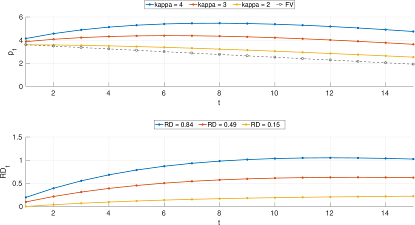
Figure 1: Equilibrium Price ($\varphi=0$) and related RD measure when $\alpha=0.85$ by varying $\kappa$. The grey line is the fundamental value dynamics. In the legend is reported the average RD measure among the parameter specifications.

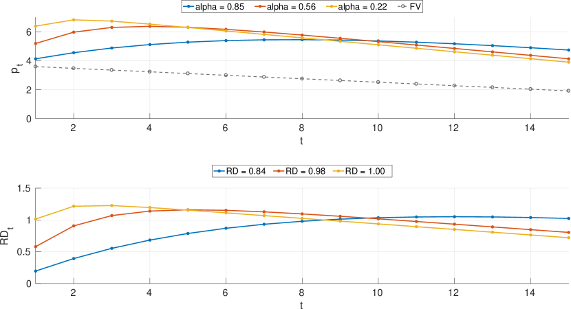
Figure 2: Equilibrium Price ($\varphi=0$) and related RD measure when $\kappa=4$ by varying $\alpha$. The grey line is the fundamental value dynamics. In the legend is reported the average RD measure among the parameter specifications.

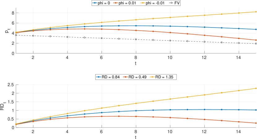
Figure 3: Average Price dynamics and related RD measure when $\kappa=4$, $\alpha=0.85$ by varying $\varphi$. The grey line is the fundamental value dynamics. In the legend is reported the average RD measure among the parameter specifications.

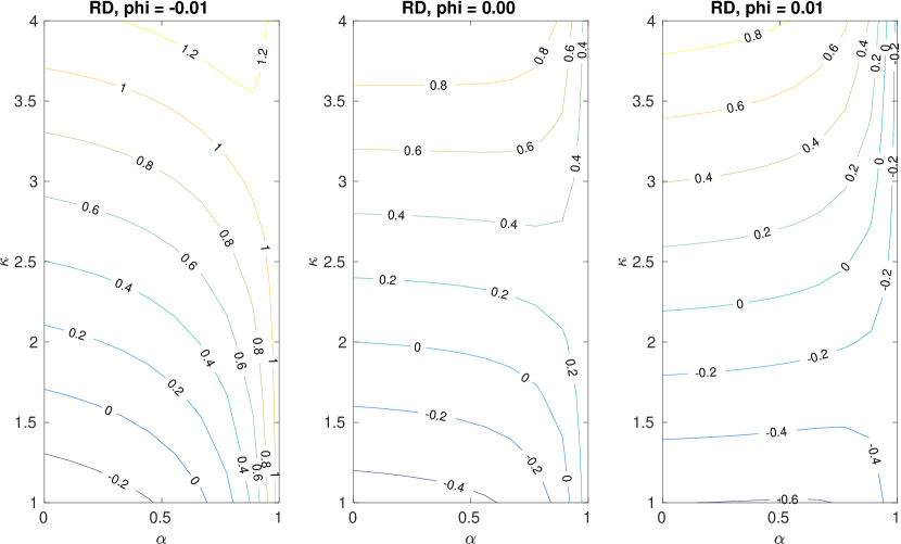
Figure 4: Contour plot of $RD$ by varying $\phi$, $\alpha$ and $\kappa$.

The overvaluation measured (at equilibrium) by RD raises when the uncertainty of traders about the fundamental value increases, i.e, when $\kappa$ increases. On the other hand, when traders are more anchoring to past prices, i.e., $\alpha$ is close to 1, overvaluation tends to decrease on average, even if it raises in the last trading rounds, see Figures 1 and 2.

We observe that when the market is at equilibrium, the price exhibits a hump-shaped dynamics in accordance with Duffy and Ünver, (2006), see Figure 3. Even if, at the middle of the market session, the price reaches a maximum, no crash is observed at the end, making the asset always overvalued. Interestingly, at the end of the market session, the average equilibrium price does not align with the fundamental value. This general overvaluation can be attributed to the noise traders’ risk described by De Long et al., (1990), where the noise traders create this difference between price and fundamental value to earn positive returns. On the other hand, when $\varphi>0$, we observed a sharp decline of the price, which is aligned with the fundamental value at the end of the market session.

Figure 4 shows the contour plot of the average RD surface among the parameters. Interestingly, by looking the curve levels in the parameter space, we observe that the weak-foresight assumption ($\varphi>0$) decreases the general overvaluation, see also Figure 3. We remark that regardless of the parameter $\varphi$ the bubble starts close to the fundamental value of the asset, precisely on average the average price of the first trading period will be equal to $FV_{1}[(1-\alpha)k/2+\alpha]$. Despite the upward trend observed by SSW and Duffy and Ünver, (2006) in the first trading periods, which is generated by traders’ inexperience, is not displayed, the price dynamics clearly exhibit the typical bubble shape. This is consistent with the analysis of Baghestanian et al., (2015) and with the results of Cordoni et al., (2022), where, even though the same noise traders of the DU model are employed the price bubbles is aligned with the fundamental value at the beginning of the trading period. This is the results of Cordoni et al., (2022) market-makers agents employed in their model to provide liquidity to the market, so that they set the average book mid-price of the first trading period to the fundamental value. Indeed, due to competitiveness, market-makers are forced to trade at efficient prices to avoid to be kicked out of the market.

4 Heterogeneous Agent Based model: Factor Investing Strategies

We consider a two-asset extension of the DU model where three types of agents are introduced: $J_{N}$ noise traders, $J_{D}$ directional and $J_{MN}$ market-neutral traders. The number of traders is equal to $J_{N}+J_{D}+J_{MN}=N$. Following Cordoni et al., (2022) we specify two model specifications for the two assets $P_{1}$ and $P_{2}$, so that we have two order books with the relative parameters, $\kappa_{i},\alpha_{i},\varphi_{i}$, for $i=1,2$. In this model we design multi-asset trading strategies mimicking factor investing style, see e.g. Li et al., (2019), which traders can implement.

The near-zero-intelligence agents of DU will be used as prototypes of noise traders. We assume that the other traders follow one of the assets, i.e., the asset $P_{1}$, to read a signal to buy or sell, i.e., $s_{1}\in\{-1,1\}$ where $1$ ($-1$) means that $s_{1}$ is a buy (sell) signal for asset $1$. As for the noise traders, the probability of reading a buy or sell signal is modelled by $\pi_{1}$, i.e., the probability of being a buyer or a seller for asset $1$. The heterogeneity is introduced by considering a percentage of agents which will follow one of the two market factors: the directional market factor $v_{D}=[1,\ 1]^{T}$ and the market-neutral market factor $v_{M}=[1,\ -1]^{T}$.

Therefore, a directional (market-neutral) trader places orders on both assets following the directional (market-neutral) market factor. Thus, an agent reads the market signal from asset one, $s_{1}$, to assign the position of buy/sell on $P_{1}$, while the position on asset $P_{2}$ depends on the market factor: if the trader is a directional (market-neutral) will place the same (opposite) order side on the other assets, i.e., the position on both assets are described by the product $s_{i}\cdot v_{D}$ ($s_{i}\cdot v_{M}$). In other words, a directional (market-neutral) trader places orders in asset 2 with the same (opposite) sign position of asset 1.

The quote sizes are the same for all agents, and they are equal to $q_{t,1}$ and $q_{t,2}$ for the two assets, respectively and they might have two distinct parameter specifications. We assume Assumption 2 for both assets, i.e., $q_{t,1}=\overline{q}_{t,1}$ and $q_{t,2}=\overline{q}_{t,2}$ for all traders. We assume that the probability of being a buyer for asset $P_{1}$ is fixed for all the traders, at trading time $t$, to $\pi_{t,1}$. The trading position on asset $2$ for noise traders is assigned by another random variable (independent from asset $P_{1}$) with a probability of being a buyer given by $\pi_{t,2}$. Since the directional and market-neutral traders will assign asset position on $P_{2}$ following the corresponding factor, there is no need to specify another random variable for their positions on asset $P_{2}.$ Therefore, we require the following assumption.

Assumption 3.

a) At the trading time $t$, all the traders decide to buy or sell asset $P_{1}$ following i.i.d. Bernoulli random variables with probability $\pi_{t,1}.$ b) At trading time $t$, the noise traders decide to buy or sell asset $P_{2}$ according to i.i.d. Bernoulli random variables with probability $\pi_{t,2}$.

Then, under Assumptions 1-2-3 we recover the equilibrium average price dynamics for the two assets. For asset $P_{1}$ traders behave as for the homogeneous case of Section 3.1. Indeed, if $p_{t,1}^{b}$ is the prevailing bid price at time $t$, then, it solves the equation

$$\sum_{j=1}^{J_{N}}\pi_{t,1}\cdot q_{t,1}+\sum_{j=1}^{J_{D}}\pi_{t,1}\cdot q_{t,1}+\sum_{j=1}^{J_{MN}}\pi_{t,1}\cdot q_{t,1}=A_{t,1}\cdot p_{t,1}^{b}$$

where $A_{t,1}$ is the supply provided by the market for asset 1 which is equal to $(1-\pi_{t,1})N$. However, $\sum_{j=1}^{J_{N}}\pi_{t,1}\cdot q_{t,1}+\sum_{j=1}^{J_{D}}\pi_{t,1}\cdot q_{t,1}+\sum_{j=1}^{J_{MN}}\pi_{t,1}\cdot q_{t,1}=N\pi_{t,1}q_{t,1}$, so that $p_{t,1}^{b}=\frac{\pi_{t,1}}{1-\pi_{t,1}}q_{t,1}$. In the same way, the prevailing ask price at time $t$, $p_{t,1}^{a}$, solves the equation

$$\sum_{j=1}^{J_{N}}(1-\pi_{t,1})\cdot q_{t,1}+\sum_{j=1}^{J_{D}}(1-\pi_{t,1})\cdot q_{t,1}+\sum_{j=1}^{J_{MN}}(1-\pi_{t,1})\cdot q_{t,1}=B_{t,1}p_{t,1}^{a}$$

where $B_{t,1}$ is the demand provided by the market which is equal to $\pi_{t,1}N$. So, $p_{t,1}^{a}=\frac{1-\pi_{t,1}}{\pi_{t,1}}q_{t,1}$. Therefore, for Asset $P_{1}$ the equilibrium price exists when $\pi_{t,1}=0.5$, and in this case it is equal to $q_{t,1}$. The average price dynamics is characterized by

$$p_{t,1}=q_{t,1}+\left(\frac{\pi_{t,1}}{1-\pi_{t,1}}-1\right).$$ (1)

For asset $P_{2}$, since $\pi_{t,2}$ is the probability to be a buyer for the noise trader, then the prevailing bid price at time $t$, $p_{t,2}^{b}$, satisfies the equation

$$\sum_{j=1}^{J_{N}}\pi_{t,2}\cdot q_{t,2}+\sum_{j=1}^{J_{D}}\pi_{t,1}\cdot q_{t,2}+\sum_{j=1}^{J_{MN}}(1-\pi_{t,1})\cdot q_{t,2}=A_{t,2}p_{t,2}^{b}$$

where $A_{t,2}$ is the supply provided by the market for asset 2 which is equal to $J_{N}(1-\pi_{t,2})+J_{D}(1-\pi_{t,1})+J_{MN}\pi_{t,1}$. We remark that the directional (market-neutral) traders have the same (opposite) side position for both assets. Solving for $p_{t,2}^{b}$, we obtain

$$p_{t,2}^{b}=\frac{J_{N}\cdot\pi_{t,2}+J_{D}\cdot\pi_{t,1}+J_{MN}\cdot(1-\pi_{t,1})}{J_{N}\cdot(1-\pi_{t,2})+J_{D}\cdot(1-\pi_{t,1})+J_{MN}\cdot\pi_{t,1}}\cdot q_{t,2}.$$

In analogous way, the prevailing ask price for asset $2$, $p_{t,2}^{a}$, solve the corresponding equation

$$\sum_{j=1}^{J_{N}}(1-\pi_{t,2})\cdot q_{t,2}+\sum_{j=1}^{J_{D}}(1-\pi_{t,1})\cdot q_{t,2}+\sum_{j=1}^{J_{MN}}\pi_{t,1}\cdot q_{t,2}=B_{t,2}p_{t,2}^{a}$$

where $B_{t,2}$ is the demand for asset 2 which is equal to $J_{N}\pi_{t,2}+J_{D}\pi_{t,1}+J_{MN}(1-\pi_{t,1})$. Thus, the prevailing ask price is equal to

$$p_{t,2}^{a}=\frac{J_{N}\cdot(1-\pi_{t,2})+J_{D}\cdot(1-\pi_{t,1})+J_{MN}\cdot\pi_{t,1}}{J_{N}\cdot\pi_{t,2}+J_{D}\cdot\pi_{t,1}+J_{MN}\cdot(1-\pi_{t,1})}\cdot q_{t,2}.$$

Therefore, if the number of directional and market-neutral traders are equal, there exists the equilibrium price for asset $P_{2}$.

Proposition 4.1.

Under Asm. 1, 2, 3 and $J_{D}=J_{MN}$, then there exists an equilibrium for asset 2 if and only if $\pi_{t,2}=0.5$ for all $t$ and $\overline{p}_{t,2}=q_{2,t}$.

We observe that when $J_{D}=J_{MN}$ the equilibrium price for the asset $P_{2}$ is independent of the probability $\pi_{t,1}$. Since $\pi_{t,2}$ represents the probability to be a buyer or seller of a noise trader, we may assume that:

Assumption 4.

$\pi_{t,2}=0.5$ for all $t.$

Then, we may drop the assumption of $J_{D}=J_{MN}$ in Proposition 4.1.

Theorem 4.2.

Under Assumptions 1, 2, 3, 4 and $J_{D}\neq J_{MN}$, then there exists an equilibrium price for asset $2$ if and only if $\pi_{t,1}=0.5$ for all $t$ and moreover $\overline{p}_{t,2}=q_{2,t}$

Theorem 4.2 implies that if $\pi_{t,1}=\pi_{t,2}=0.5$ there exists an equilibrium for both assets, and it is determined by the respective quotes, $q_{t,1}$ and $q_{t,2}$. Moreover, under Assumption 4, the imbalance between demand and supply for asset 2 is equal to

$$\frac{J_{N}\cdot 0.5+J_{D}\pi_{t,1}+J_{MN}(1-\pi_{t,1})}{J_{N}\cdot 0.5+J_{D}(1-\pi_{t,1})+J_{MN}\pi_{t,1}}-1.$$

Then, under the previous assumptions, the average price dynamic for the two asset is given by

$$\begin{split}p_{t,1}&=q_{t,1}+\left(\frac{\pi_{t,1}}{1-\pi_{t,1}}-1\right)\\ p_{t,2}&=q_{t,2}+\left(\frac{J_{N}\cdot 0.5+J_{D}\pi_{t,1}+J_{MN}(1-\pi_{t,1})}{J_{N}\cdot 0.5+J_{D}(1-\pi_{t,1})+J_{MN}\pi_{t,1}}-1\right).\end{split}$$ (2)

In Figure 5 shows the RD comparison among the two-assets for different model specifications. We select the assets dividend support as presented in Section 2. We follow the experiment design of Cordoni et al., (2022), setting the other parameters to $\kappa_{1}=4$, $\kappa_{2}=2$. We set $\alpha_{1}=\alpha_{2}=0.85$ and for the equilibrium dynamics, $\pi_{1}=\pi_{2}=0.5$. Then, we consider the case when asset $1$ is no longer in equilibrium, i.e., $\varphi_{1}=0.01\leavevmode\nobreak\ 0.25/T>0$, for $J_{D}=J_{MN}$, $J_{D}=45>J_{MN}=5$ and $J_{D}=5<J_{MN}=45$. In both cases the number of noise traders is fixed to $J_{N}=50.$

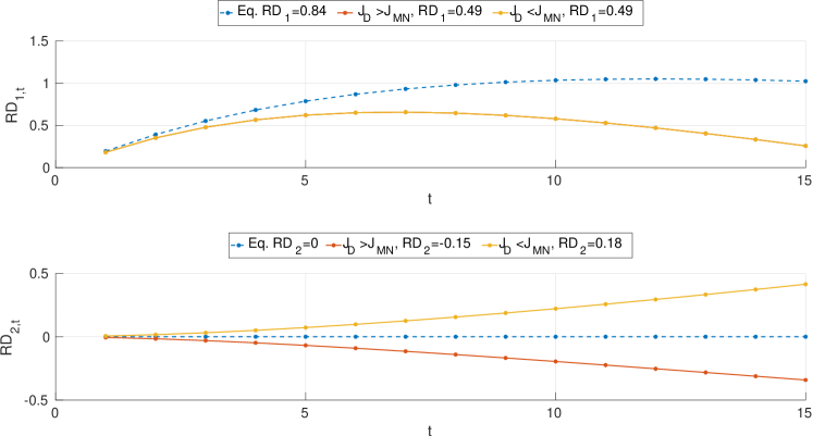
Figure 5: $RD_{i,t}$ for two-asset markets. Equilibrium prices are obtain for $\varphi_{1}=0$ (blue dotted lines), and $\varphi_{1}=0.01$ in other case (solid lines). $\kappa_{1}=4$, $\kappa_{2}=2$, $\alpha_{1}=\alpha_{2}=0.85$ and $J_{D}(\%)+J_{MN}(\%)=50\%$. Red (Orange) lines refer when $J_{D}>J_{MN}$ ($J_{D}<J_{MN}$). The average RD, respectively for each case, is reported in the legend bar. In the top exhibit, the $RD_{1,t}$ coincides when $J_{D}>J_{MN}$ and $J_{D}<J_{MN}$.

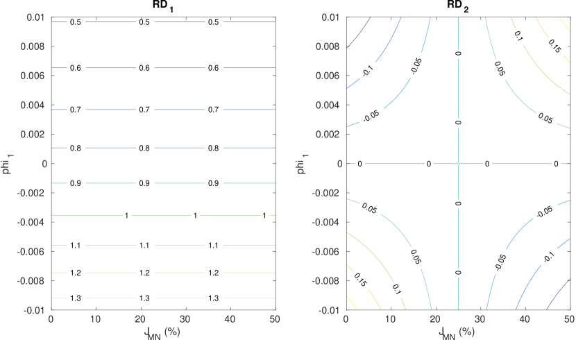
Figure 6: RD for two-asset markets when we vary $\pi_{1}$ and $J_{MN}$. $\kappa_{1}=4$, $\kappa_{2}=2$, $\alpha_{1}=\alpha_{2}=0.85$ and $J_{D}(\%)+J_{MN}(\%)=50\%$.

From Figure 5 and the contour plot in Figure 6, we observe that when asset 2 is in equilibrium, its price coincides with its fundamental value, i.e., $RD_{2}=0$, regardless of any parameter setting of $P_{1}$. Thus, there is no effect of price bubble contagion of asset $P_{1}$ toward asset $P_{2}$. Moreover, according to Proposition 4.1, from the right exhibit of Figure 6 we may observe how the misvaluation is zero when $J_{D}=J_{MN}$ regardless if the asset $P_{1}$ is in equilibrium, i.e. $\varphi>0$. Furthermore, we may also observe how the misvaluation of asset $P_{1}$ is invariant from the percentual of directional and market-neutral traders.

On the other hand, when $\varphi_{1}>0$ and $\pi_{2}=0.5$, we observe that the price bubble of asset $P_{1}$ affects the dynamics of asset $P_{2}$ when the proportion between directional and market-neutral traders is varying, generating a misvaluation effect. In particular, when there are more market-neutral agents in the market than directional traders, the bubble of $P_{1}$ triggers a “overvaluation” effect also for asset $P_{2}$, by positively deviating the price from its fundamental value. Viceversa, when $J_{D}>J_{MN}$ we observe an “undervaluation” effect for $P_{2}$. These findings are consistent with what was observed in the simulation study of Cordoni et al., (2022).

For both Figures 5 and 6, we observe that when the market is not in equilibrium, the price-bubble, i.e., asset $P_{1}$, exhibits a sharp decline at the end of the session aligning with the fundamental value.

5 Equilibrium Price for Heterogeneous Agent-Based model with investment strategies

The parameter $\varphi>0$ plays a crucial role in the DU model in order to get consistent results with the experimental data. It reduces the transaction volume over time consistent with the experimental data through the weak foresight assumption. The DU model relies on this assumption to generate the observed crash patterns of the laboratory market experiments. However, this artificial hypothesis is nothing else than a pure statistical condition that guarantees a progressively decreasing prices and volume transactions in an exogenous way. We now drop this assumption by considering the heterogeneous model of Baghestanian et al., (2015) and analyzing the corresponding equilibrium price dynamics in a two-asset market employing (endogenous) investment strategies.

We first present the model for a generic asset (without specifying the subscript index), and then we specify how we extend these strategies to the two-asset market. We consider three types of agents: $J_{N}$ noise traders, $J_{F}$ fundamentalist and $J_{S}$ speculative traders. The number of traders is set to $J_{N}+J_{F}+J_{S}=N$. The fundamentalist and speculative traders track the fundamental value and past prices to decide their position. Their quotes size are denoted by $q_{t}^{F}$ and $q_{t}^{S}$, respectively.

The fundamentalists compute in every trading period $t$ a measure linked to the fundamental value and past trading price, $l_{t}=\alpha^{F}l_{t-1}+(1-\alpha^{F})p_{t-1}-\overline{d}$, where $\alpha^{F}\in(0,1)$ and $l_{0}=FV_{1}+\overline{d}$. If $l_{t}\leq FV_{t}$ they decide to submit a buy order otherwise they submit a sell order. The quote size, under Assumption 1 and 2, is on average

$$q_{t}^{F}=\frac{l_{t}+FV_{t}}{2}.$$

The speculative traders decide whether to buy or sell depending on their expectations about clearing prices in period $[t,t+1[$ at the beginning of the trading period $t$. Speculative traders form expectations following the rule:

$$E_{p_{t}}=\gamma_{1}p_{t-1}+\gamma_{2}FV_{t},\gamma_{1}\in[0,1],\ \gamma_{2}\geq 0.$$

Iterating one period forward we may obtain $E_{p_{t+1}}$ in function of $FV_{t},FV_{t+1},p_{t-1},p_{t-2}$, If $E_{p_{t+1}}>E_{p_{t}}$ the speculator will post a bid otherwise he/she will post an ask. Their quotes, under Assumption 1 and 2, are on average

$$q_{t}^{S}=\frac{E_{p_{t+1}}+E_{p_{t}}}{2}.$$

The quote sizes for noise agents are equal to $q_{t}=(1-\alpha)u_{t}+\alpha\overline{p}_{t-1}$, where $u_{t}\sim U(0,\kappa FV_{t})$, with the same rule of the DU model. Therefore, let $p_{t}^{b}$ and $p_{t}^{a}$ the prevailing bid and ask price

$$\sum_{j=1}^{J_{N}}\pi_{t}q_{t}+\sum_{j=1}^{J_{F}}1_{l_{t}\leq FV_{t}}q_{t}^{F}+\sum_{j=1}^{J_{S}}1_{E_{p_{t+1}}>E_{p_{t}}}q_{t}^{S}=A_{t}p_{t}^{b}$$

$$\sum_{j=1}^{J_{N}}(1-\pi_{t})q_{t}+\sum_{j=1}^{J_{F}}1_{l_{t}>FV_{t}}q_{t}^{F}+\sum_{j=1}^{J_{S}}1_{E_{p_{t+1}}\leq E_{p_{t}}}q_{t}^{S}=B_{t}p_{t}^{a}$$

On average, noise traders act as liquidity providers for fundamentalists and speculators and we may assume that $J_{N}\geq J_{F}+J_{S}$, where the probability to buy an asset, $\pi_{t}$, for noise traders is equal to $0.5$. The equilibrium is recovered when $J_{F}=J_{S}=0$, and in this case, the model is exactly the DU model, where the average equilibrium price is equal to $\overline{p}_{t}=q_{t}$, see also the discussion in Baghestanian et al., (2015).

5.1 A theoretical motivation of Price Bubble in Experiments

We now combine the previous equilibrium results and trader investment strategies to motivate the typical hump-shaped price during market experiments. We explain the behaviour discussed in Baghestanian et al., (2015) from a theoretical point of view, analyzing the trading events which lead to price bubbles shape.

When $J_{F}+J_{S}>0$, we compute the relative order imbalance that characterizes the price dynamics. However, we have to consider four possible events and compute for each event the corresponding imbalance. The events corresponds to when the fundamentalists and speculators are buyer and/or seller. In event $E_{1}=\{l_{t}\leq FV_{t},E_{p_{t+1}}\leq E_{p_{t}}\}$, fundamentalists will buy and speculators will sell, in $E_{2}=\{l_{t}\leq FV_{t},E_{p_{t+1}}>E_{p_{t}}\}$, both fundamentalists and speculators will buy, while $E_{3}=\{l_{t}>FV_{t},E_{p_{t+1}}\leq E_{p_{t}}\}$ both fundamentalists and speculators will sell, and finally in $E_{4}=\{l_{t}>FV_{t},E_{p_{t+1}}>E_{p_{t}}\}$ fundamentalists will sell and speculators will buy. Then, respectively for each event, we may derive the demand and supply imbalance,

$$\begin{split}E1&:\begin{cases}A_{t}&=J_{N}(1-\pi_{t})+J_{S}\\ B_{t}&=J_{N}\pi_{t}+J_{F}\end{cases},\text{ then }\frac{B_{t}}{A_{t}}-1=\frac{0.5J_{N}+J_{F}}{0.5J_{N}+J_{S}}-1.\\ E2&:\begin{cases}A_{t}&=J_{N}(1-\pi_{t})\\ B_{t}&=J_{N}\pi_{t}+J_{F}+J_{S}\end{cases},\text{ then }\frac{B_{t}}{A_{t}}-1=\frac{0.5J_{N}+J_{F}+J_{S}}{0.5J_{N}}-1=2\frac{J_{F}+J_{S}}{J_{N}}\\ E3&:\begin{cases}A_{t}&=J_{N}(1-\pi_{t})+J_{F}+J_{S}\\ B_{t}&=J_{N}\pi_{t}\end{cases},\text{ then }\frac{B_{t}}{A_{t}}-1=\frac{0.5J_{N}}{0.5J_{N}+J_{F}+J_{S}}-1\\ E4&:\begin{cases}A_{t}&=J_{N}(1-\pi_{t})+J_{F}\\ B_{t}&=J_{N}\pi_{t}+J_{S}\end{cases},\text{ then }\frac{B_{t}}{A_{t}}-1=\frac{0.5J_{N}+J_{S}}{0.5J_{N}+J_{F}}-1.\end{split}$$

The price dynamics is path-dependent and characterized by the parameters of the fundamentalist and speculative traders. Therefore, at the end of each time step, we have to compute the position and beliefs of fundamentalists and speculators to decide which one of the events we are and compute the corresponding demand and supply imbalance. Trivially, the imbalance pushes up and down prices depending on the number of fundamentalists and speculators. We characterize the price dynamics by recovering the bid and ask prices due to the average quotes among noisy, fundamentalists and speculators quotes depending on the event realization. We recall that the market is in equilibrium when $p_{t}^{a}=p_{t}^{b}$. The price dynamics of (prevailing) ask and bid can be expressed among the events in the following way,

$$\begin{split}E1&:\begin{cases}p_{t}^{a}&=\frac{0.5J_{N}q_{t}+J_{S}q_{t}^{S}}{0.5J_{N}+J_{F}}\\ p_{t}^{b}&=\frac{0.5J_{N}q_{t}+J_{F}q_{t}^{F}}{0.5J_{N}+J_{S}}\end{cases},\quad E2:\begin{cases}p_{t}^{a}&=\frac{0.5J_{N}q_{t}}{0.5J_{N}+J_{F}+J_{S}}\\ p_{t}^{b}&=\frac{0.5J_{N}q_{t}+J_{F}q_{t}^{F}+J_{S}q_{t}^{S}}{0.5J_{N}}\end{cases},\\ E3&:\begin{cases}p_{t}^{a}&=\frac{0.5J_{N}q_{t}+J_{F}q_{t}^{F}+J_{S}q_{t}^{S}}{0.5J_{N}}\\ p_{t}^{b}&=\frac{0.5J_{N}q_{t}}{0.5J_{N}+J_{F}+J_{S}}\end{cases},\quad E4:\begin{cases}p_{t}^{a}&=\frac{0.5J_{N}q_{t}+J_{F}q_{t}^{F}}{0.5J_{N}+J_{S}}\\ p_{t}^{b}&=\frac{0.5J_{N}q_{t}+J_{S}q_{t}^{S}}{0.5J_{N}+J_{F}}\end{cases},\end{split}$$

When $J_{N}\to\infty$ ( and $J_{F}+J_{S}$ is bounded) the average price dynamics will converge on the equilibrium price $\overline{p}_{t}=q_{t}$, dotted blue lines of Figure 7, top panel, characterized by noise traders’ activity, otherwise, the average price dynamics will be determined by the (mid-)price formed by the interaction of all traders, noise, fundamentalists and speculators, red lines of Figure 7, top panel. We may formalize the previous statement as follow. Let $\overline{p}_{t}^{Het}$ and $\overline{p}_{t}^{Hom}$ denote the average market-clearing price of the heterogeneous and homogeneous model, respectively.

Proposition 5.1.

Under Assumptions 1, 2 and previous model specifications, if $J_{F}+J_{S}$ is bounded, when $J_{N}\to\infty$ the market is in equilibrium and the average market-clearing price of the heterogeneous model will converge on the equilibrium market-clearing price of the homogeneous model, i.e., $\overline{p}_{t}^{Het}\to\overline{p}_{t}^{Hom}$.

Figure 7 exhibits the average mid-price and equilibrium price dynamics by computing the ask and bid together with the order and cumulative imbalance. The noise trader quotes are updated using the previous period mid-price, i.e., $q_{t}=(1-\alpha)\overline{u}_{t}+\alpha(p^{a}_{t-1}+p^{b}_{t-1})/2$. The average equilibrium price $\overline{p}_{t}$ is computed recursively, $\overline{p}_{t}=(1-\alpha)\overline{u}_{t}+\alpha\overline{p}_{t-1}$, where $\overline{p}_{0}=FV_{1}.$ We set $\kappa=4$, $\alpha=0.85$, $J_{N}=50$, $J_{F}=6$ and $J_{S}=4$, $\alpha^{F}=0.25$, $\gamma_{1}=0.10$ and $\gamma_{2}=4$. The parameters are consistent with the estimates provided by Duffy and Ünver, (2006) (for the noise traders parameter) and Baghestanian et al., (2015) (for the fundamentalists and speculators). We select the asset dividend support of $P_{1}$ as in Section 2.

The price dynamics exhibits the typical hump price-bubble shape. As observed by Baghestanian et al., (2015), assuming that $J_{F}>J_{S}$, when $\alpha^{F}<1$ and $\gamma_{1}>0$ the initial phase is characterized by an accumulation of shares. In Baghestanian et al., (2015) fundamentalists buy from speculators and noise traders, i.e., we are in event E1. From the bid/ask imbalance, $\frac{0.5J_{N}+J_{F}}{0.5J_{N}+J_{S}}-1$, we may observe that the price is pushed forward. However, as discussed in Smith et al., (1988), Duffy and Ünver, (2006) agents start trading the stock at a low value compared to the fundamental due to inexperience. Thus, by assuming that $\overline{p}_{0}=FV_{1}$, we are implicitly assuming that traders are in some way experienced enough to correctly compute the fundamental value at time $t=1$. Therefore, in our setting the first event which is realized is event E2, where fundamentalists together with speculators decide to buy, see Figure 7, and traders generate an upward trend with a subsequent soaring of the price dynamics. This triggers the boom phase, where the price is pushed away from the fundamental value with an imbalance equal to $2\frac{J_{F}+J_{S}}{J_{N}}$. Thus, since the price will be far away from the fundamental value, the fundamentalists decide to sell to the speculators and noise traders, event E4. This event is realized in the middle of the trading session until the price reaches its peak. Then, the price starts its decline pushed down by the imbalance $\frac{0.5J_{N}+J_{S}}{0.5J_{N}+J_{F}}-1$. Subsequently, also, speculators start to sell together with fundamentalist, i.e., we are in event $E3$, the burst phase, with a consequent liquidity drop fulfilled by noise traders, which causes the price-bubble crash, supported by the imbalance of $\frac{0.5J_{N}}{0.5J_{N}+J_{F}+J_{S}}-1$. Speculators start to sell since it decreases the traders subjectively perceived probability of being able to sell (Smith et al., , 1988, Duffy and Ünver, , 2006, Baghestanian et al., , 2015). The burst phase starts when the cumulative imbalance becomes negative, see bottom panel of Figure 7.

We observe that during events E2 and E4, the spread is closed, i.e., $p_{t}^{a}\leq p_{t}^{b}$ generating the equilibrium price, until event E3 starts where the spread will be open. In this phase we may consider the equilibrium mid-price dynamics, which is determined by noise traders’ orders which are executed inside the spread between $p_{t}^{b}$ and $p_{t}^{a}$.

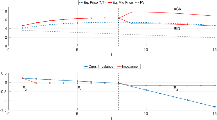
Figure 7: Equilibrium average price and order imbalance. (Top panel) Average mid-price (red) and equilibrium (blue dotted lines) price dynamics from the heterogeneous model of Baghestanian et al., (2015). The dashed grey lines split the trading period depending on the realized event, which characterized the order imbalance (Bottom panel).

As observed also in Section 3.1, the average equilibrium mid-price does not converge to the fundamental value, even if fundamentalists and speculators agents are included in the market. Indeed, as explained by De Long et al., (1990), this phenomenon may be attributed to the noise traders’ risk, which discourages other rational agents from facing noise traders, causing so this significant deviation of the price from fundamental value.

5.2 The Two-Asset Case

We analyse the equilibrium price affected by different investment strategies in a multi-asset scenario. We recall that we focus on the assets fundamental values discussed in Section 2, where $\overline{d}_{1}>0$ and $\overline{d}_{2}=0.$

We consider for the moment the dynamics of asset $P_{1}$. For the sake of notation, we will not report the subscript $1$, since the below reasoning is valid for a generic asset with $\overline{d}\geq 0$. We restrict our analysis in the limit case of $\alpha^{F}=1$ and $\gamma_{1}=0$ when both fundamentalists and speculators follow one of the market factors discussed in Section 4.

Therefore, $l_{t}=FV_{t}$ for all $t$ and $E_{p_{t}}=\gamma_{2}FV_{t}$ is decreasing in time, when $FV_{t}$ is decreasing. Traders follow asset 1 and decide the position on asset 2 using the respective factor. For a generic asset $i$, we recall that a fundamentalist decides to buy if $l_{t,i}\leq FV_{t,i}$ and a speculator decides to sell if $E_{p_{t,i}}\geq E_{p_{t+1,i}}$. Thus, for all $t$ fundamentalist will buy asset $P_{1}$ while speculator will sell it, i.e., event $E_{1}$ is realized for asset $P_{1}$. Moreover, $q_{t}^{F}=FV_{t}$ and $q_{t}^{S}=\frac{\gamma_{2}}{2}(FV_{t}+FV_{t+1})=\frac{\gamma_{2}}{2}(FV_{t}+FV_{t}-\overline{d})=\gamma_{2}(FV_{t}-\frac{1}{2}\overline{d})$. Therefore,

$$\begin{cases}p_{t}^{a}&=\frac{0.5J_{N}q_{t}+J_{S}\gamma_{2}(FV_{t}-\frac{1}{2}\overline{d})}{0.5J_{N}+J_{F}}\\ p_{t}^{b}&=\frac{0.5J_{N}q_{t}+J_{F}FV_{t}}{0.5J_{N}+J_{S}}.\end{cases}$$ (3)

We now proof the following results, under the assumption that $J_{F}=J_{S}$.

Proposition 5.2.

When fundamentalists and speculator agents form expectations for the next market-clearing price without considering the previous trading period price, i.e., $\alpha^{F}=1$ and $\gamma_{1}=0$, then if $J_{F}=J_{S}$, $p_{t}^{a}>p_{t}^{b}$ if and only if $\gamma_{2}>\frac{2FV_{t}}{2FV_{t}-\overline{d}}\ \forall t$.

Therefore, fundamentalists and speculators sustain the demand and supply regardless of noise traders. On the other hand, the price dynamics is mainly led by noise traders who execute orders inside the spread formed by fundamentalists and speculators. On average, the mid-price $p_{t}$ will characterize the dynamics of the price realizations outlined by $p_{t}^{b}$ and $p_{t}^{a}$ quotes. We may consider $p_{t}$ as the benchmark price realizations used by noise traders when they post their quotes $q_{t}$. Therefore, under the previous assumptions, the mid-price dynamics of asset $P_{1}$ is given by

$$p_{t}=\frac{p_{t}^{a}+p_{t}^{b}}{2}=\frac{J_{N}q_{t}+J_{F}(FV_{t}+\gamma_{2}(FV_{t}-\frac{\overline{d}}{2}))}{J_{N}+2J_{F}},$$

$$p_{t}=\frac{J_{N}(\kappa\frac{FV_{t}}{2}(1-\alpha)+\alpha p_{t-1}))+J_{F}(FV_{t}+\gamma_{2}(FV_{t}-\frac{\overline{d}}{2}))}{J_{N}+2J_{F}}.$$ (4)

We remark that, following the same above reasoning, we may obtain the price description also for asset $P_{2}$, see Section 5.2.2.

5.2.1 Factor Investing and Investment Strategies

We now combine the Baghestanian et al., (2015) model and the two-assets generalization with market factors of Section 4, where the fundamental value of the first asset is declining among the periods while the second one is constant. We first assume that fundamentalist and speculator agents follow asset $P_{1}$ and read the signal to decide the position on the second asset. The signal reads by the agents differ according to the investment strategies followed by agents in the first asset. For instance, if $l_{t,1}\leq FV_{t,1}$ fundamentalists decide to buy the first asset and buy or sell the second asset depending on the selected market factors, $v_{D}$ or $v_{M}$. Noise traders place orders randomly for both assets. Although fundamentalist and speculator traders place a quote on asset $P_{1}$ following their strategies, we have to decide what are the quotes they will post on the other asset $P_{2}$. Thus, we make the following assumption.

Assumption 5.

For all traders, the quotes on the second asset follow those of noise agents, i.e., on average $q_{t,2}=(1-\alpha_{2})\frac{\kappa_{2}}{2}FV_{t,2}+\alpha_{2}p_{t-1,2}$.

Therefore, using the same argument of Section 4 the price dynamics of $p_{t,2}$ will be of the form $q_{t,2}+(B_{t}/A_{t}-1).$ The demand and supply imbalance depends on the market factors followed by traders and on the parameter specification of both fundamentalists and speculators. As previously done, we assume that $\alpha^{F}=1$, $\gamma_{1}=0$ and $J_{F}=J_{S}$. Therefore, fundamentalists and speculators will buy and sell, respectively the first asset. If they select the same factor, i.e., they are both directionals or market neutrals, the price dynamics of asset $P_{2}$ is in equilibrium and $p_{t,2}=q_{t,2}$.

Theorem 5.3.

Under Assumptions, 1, 2, 3-b, 4, 5, in the two assets generalization, when fundamentalists and speculators decide position on the second asset selecting a market factor, they form expectations for the next market-clearing price without considering the previous trading period price, i.e., $\alpha^{F}=1$, $\gamma_{1}=0$, and $J_{F}=J_{S}$ and both fundamentalists and speculators select the same factor, the price dynamics of asset $P_{2}$ is in equilibrium and it is given by $p_{t,2}=q_{t,2}.$

In Figure 8 we display the average mid-price for both asset where the parameter are setting to $\kappa_{1}=4$, $\kappa_{2}=2$, $\alpha_{1}=\alpha_{2}=0.85$, $J_{N}=50$, $J_{S}=J_{F}=25$, $\alpha^{F}=1$, $\gamma_{1}=0$, $\gamma_{2}=4$ and both the fundamentalists and speculators follow the same factor (i.e., when they are both directionalists or they are both market-neutrals, since we obtain exactly the same price dynamics). The dividend distribution are the same described in Section 2. From Theorem 5.3 asset $P_{2}$ is in equilibrium which coincides with the fundamental value. We display the average mid-price dynamics since from Proposition 3 $p^{b}_{t,1}<p_{t,2}^{a}$ and the price dynamics is characterized by noise traders orders which are executed inside the spread formed by fundamentalists and speculators.

Figure 8: Average mid-price for two-asset markets by varying the percentage of noise traders $J_{N}$, from the heterogeneous model of Baghestanian et al., (2015) when both fundamentalist and speculators follow the same factor (directional or market-neutral). $\kappa_{1}=4$, $\kappa_{2}=2$, $\alpha_{1}=\alpha_{2}=0.85$, $\alpha^{F}=1$, $\gamma_{1}=0$, $\gamma_{2}=4$ and $J_{S}=J_{F}=(1-J_{N})/2=25$. For each trading period we compute the current ask and bid price, depending on the event realization. The noise trader quotes are updated using the previous period mid-price, i.e., $q_{t}=(1-\alpha)\overline{u}_{t}+\alpha(p^{a}_{t-1}+p^{b}_{t-1})/2$. The fundamental value is shown in blue dotted lines.

Moreover, the misvaluation of generated by the price bubble, $P_{1}$, decreases when the percentage of noise traders, $J_{N}$, increases, see also the RD measures in Figure 9. On the other hand, the misvaluation of asset $P_{2}$ is invariant from $J_{N}$. However, when traders’ confusion on the fundamental value of asset $P_{2}$ increases, i.e., the parameter $\kappa_{2}$, the price is still in equilibrium but it exhibits the price bubble shape and a subsequent significant overvaluation.

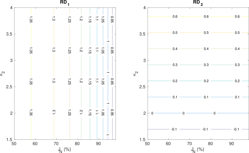
Figure 9: RD for two-asset markets when the percentage of noise traders, $J_{N}$, and traders’ confusion about the fundamental value of asset $P_{2}$, i.e., $\kappa_{2}$, are varying.

Regardless the market factors, for asset $P_{1}$, the event $E1$ is realized, while for asset $P_{2}$, when traders follow the directional (market-neutral) factor, the event $E1$ ($E4$) is realized, respectively. When fundamentalists and speculators follow opposite market factors, the price dynamics of asset 2 is no longer in equilibrium, and it is driven by the demand and supply imbalance of event $E_{2}$ or $E_{3}$, depending on if the fundamentalists/speculators are directional/market-neutral or market-neutral/directional, respectively.

The previous result highlights an identification issue since the price equilibrium is reached when fundamentalists and speculators follow the directional or market-neutral factor. Thus, is the equilibrium characterised by the directional or market-neutral factor? The next section will propose a possible economic motivation, to identify one of the two-factor strategies characterizing the equilibrium and solving the previous identification problem. In particular, we will specify an investment strategy also for asset $P_{2}$ and we will also relax Assumption 5.

5.2.2 Solving the identification problem of factor-investing equilibrium

We now investigate a possible economic interpretation of the previous results. To do that, we have to extend the Baghestanian et al., (2015) model to the two-assets case without relying on market factors.

We now assume that a trader who follows a particular investment strategy for the first asset, e.g., the fundamentalist one, uses the same strategy also for the second asset. This assumption will replace the more constraining Assumption 5.

Assumption 6.

A fundamentalist (speculative) trader for asset $P_{1}$ is also a fundamentalist (speculative) for the second asset.

The parameters of investment strategies differ for the two assets, and we generalize the previous model specification using $\alpha^{F}_{i}$ as the fundamentalist anchoring parameter for asset $i$ and $\gamma_{1,i}$ and $\gamma_{2,i}$ as the parameters used by speculators to form expectations about next market-clearing price for asset $i$. The quote size for the two assets is trivially the average of the corresponding clearing prices expectations.

Thus, we may assume as for asset $1$ that fundamentalists and speculator agents form expectations for the next market-clearing price for asset $P_{2}$ without considering the previous trading period price, i.e., $\alpha^{F}_{2}=1$ $\gamma_{1,2}=0$.

Theorem 5.4.

Under Assumptions, 1, 2, 3-b, 4, 6, if $\overline{d}_{2}=0$, $J_{F}=J_{S}$, when fundamentalists and speculator agents form expectations for the next market-clearing price without considering the previous trading period price for both assets, i.e., $\alpha_{\cdot}^{F}=1$ and $\gamma_{1,\cdot}=0$, then the price of asset $2$ is in equilibrium if and only if $\gamma_{2,2}=1.$

Thus, following the same reasoning of the proof of Theorem 5.3, fundamentalists decide to buy while speculators decide to sell asset $P_{2}$, i.e., they have the same position they have for asset $P_{1}$. This kind of demand and supply entanglement is the same as for the previous factor investing strategies model where agents follow the directional market factor.

The average price dynamics generated by the model where fundamentalist and speculators follows the same strategies for both asset (without relying on factors) where $\kappa_{1}=4$, $\kappa_{2}=2$, $\alpha_{1}=\alpha_{2}=0.85$, $J_{N}=50$, $J_{S}=J_{F}=25$, $\alpha^{F}_{1}=\alpha^{F}_{2}=1$, $\gamma_{1,1}=\gamma_{1,2}=0$, $\gamma_{2,1}=4$ and $\gamma_{2,2}=1$ coincides exactly with those exhibited by Figure 8, where fundamentalists and speculators use the same factor strategies (which can be directional or market-neutral) for asset $P_{2}$. Moreover, under the model specification considered above, fundamentalists and speculators post the same quotes, i.e., $q_{t}^{F}=q_{t}^{S}=FV_{t}$. The price dynamics of asset $P_{2}$ is characterized by a weighted average of the quote of noise traders and that of fundamentalists and speculators, i.e., from Equation (4) and recalling that $FV_{t,2}$ is constant among trading periods we obtain that

$$p_{t,2}=\frac{J_{N}(FV_{t,2}\frac{\kappa_{2}}{2}(1-\alpha_{2})+\alpha_{2}p_{t-1,2})+2J_{F}FV_{t,2}}{J_{N}+2J_{F}}$$

Therefore, when noise traders have no confusion on $FV_{2}$, i.e., $\kappa_{2}=2$, since $p_{0,2}=FV_{1,2}=FV_{t,2}$ we may relate the equilibrium found in Theorem 5.3 to the previous one.

In other words, by extending the Baghestanian et al., (2015) in the two-asset case, we can identify the two-assets equilibrium described by Theorem 5.3, see Figure 10. The two-asset equilibrium described in Theorem 5.3 can be reached by two paths. By assuming the model where fundamentalists/speculators follow the market-neutral factor for posting their quotes on asset $P_{2}$, model $\mathscr{M}^{spec,mn}_{fund,mn}$, or by assuming that they follow the directional, model $\mathscr{M}^{spec,direc}_{fund,direc}$. However, from Theorem 5.4 we know that when both fundamentalists and speculators follow the same investments strategies for both assets, i.e., they are fundamentalists and speculators also for asset $P_{2}$, respectively, model $\mathscr{M}^{spec,spec}_{fund,fund}$, we generate the same order imbalance between demand and supply obtained by model $\mathscr{M}^{spec,direc}_{fund,direc}$. Indeed, for both asset event E1 is realized and we obtain exactly the same two-asset equilibrium and order imbalance.

Figure 10: An economic motivation of the two-assets equilibrium. $\mathscr{M}^{spec,spec}_{fund,fund}$ stands for the model when both fundamentalists and speculators follow the same investments strategies for both assets, i.e., they are fundamentalists and speculators also for asset $P_{2}$, respectively. $\mathscr{M}^{spec,direc}_{fund,direc}$ ($\mathscr{M}^{spec,mn}_{fund,mn}$) stands for the model where fundamentalists/speculators follow the directional (market-neutral) factor for posting their quotes on asset $P_{2}$.

Finally, we observe that when the price of asset $P_{2}$ is not in equilibrium, $\gamma_{2,2}\neq 1$, the overvaluation measured by RD decreases when the percentage of noise traders $J_{N}$ increases as observed for asset $P_{1}$, see Figure 11. On the other hand, the overvaluation of the price bubble of asset $P_{1}$ remains invariant when we vary the speculators’ perception (confusion) about the fundamental value of asset $P_{2}$, i.e., $\gamma_{2,2}$.

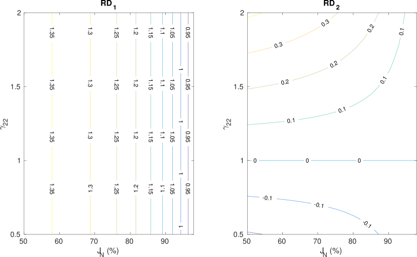
Figure 11: RD for two-asset markets when the percentage of noise traders, $J_{N}$, and speculators’ perception about the fundamental value of asset $P_{2}$, i.e., $\gamma_{2,2}$, are varying. The other parameters are set to $\kappa_{1}=4$, $\kappa_{2}=2$, $\alpha_{1}=\alpha_{2}=0.85$, $\alpha^{F}_{\cdot}=1$, $\gamma_{1,\cdot}=0$, $\gamma_{2,1}=4$ and $J_{S}=J_{F}=(1-J_{N})/2$.

In conclusion, if in Theorem 5.3 we have highlighted an identification issue due to the possibility of reaching equilibrium with two different factor investing strategies, now this identification problem is resolved. Even if the fundamental value dynamics are different, the price of asset $P_{2}$ reaches an equilibrium when agents follow the same investment strategy for both assets. Then, the equilibrium is reached using the directional market factor strategy since fundamentalists will also buy asset $P_{2}$ while speculators will sell it, following the same demand and supply imbalance of asset $P_{1}$.

6 Conclusion

This work shows the existence of price equilibria for various agent-based models to investigate the origin of the typical price-bubble mechanism observed in experimental asset markets. The equilibrium prices dynamics exhibit price-bubbles shape for those assets with a positive average dividend consistently with the experimental asset literature, e.g., Smith et al., (1988), Caginalp et al., (2002), Kirchler et al., (2012). When the market is not at equilibrium, a sharp decline in the price-bubble is observed at the end of market session, which triggers a price deviation from the fundamental value of the other asset. This contagion/misvaluation effect is also displayed in the experiments of Caginalp et al., (2002), where price bubbles tend to increase the volatility of other assets, and in the simulation results of Cordoni et al., (2022), where the price bubble triggers asymmetric cross-impact effects.

Starting from the homogeneous DU agent-based model, we show how the price equilibrium is characterized by the so-called weak-foresight assumption. Our analysis is then extended to the two-asset case discussing how the equilibrium can be reached in the presence of heterogeneous agents when factor-investing and investment strategies are introduced. We have shown necessary and sufficient conditions for which the price dynamics exhibits average bubble-crash patterns typically observed in experimental economics. The analytical expression, from which the average price dynamics for both assets can be recovered, is also derived.

We have highlighted how, under generic assumptions, the equilibrium in the two-asset extension can be reached in two alternative factor investing trading strategies, generating an identification problem. However, by extending the model of Baghestanian et al., (2015) in a two-asset market, this identification issue is solved, finding motivation for describing how the equilibrium can be reached.

Our work can be extended in many directions. We could consider the multi-asset extension (with more than two assets) or consider different market participants as market-maker agents and study their impact on the equilibrium price dynamics. Moreover, through market experiments, we could validate agent-based models considered and study the causes and effects of how particular dynamics might arise in a laboratory asset market. We are currently developing these experiments involving humans (professionals and students) and artificial agents in upcoming works.

Finally, the presented results might be helpful to experimental design and hypotheses formulation. For instance, by employing one of the model specifications, we might figure out whether, on average, price bubbles will occur or not in a determined market setting. Therefore, an experiment may be calibrated to prevent the bubble-crash pattern by exploiting our average equilibrium price dynamics analyses.

Appendix A Proofs of the results.

Proof of Lemma 3.1.

We first observe that the random quantity $u_{t}$ satisfies $u_{t}\leq\kappa FV_{t}<\kappa FV_{0}$, since $FV_{t}$ is decreasing over time. Then, since the quote $q_{t}$ is a weighted average of the previous trading price, $\overline{p}_{t-1}$ and $u_{t}$, where $\overline{p}_{0}=FV_{0}$, we can easily conclude by induction that $q_{t}<\kappa FV_{0}$. Indeed, since $\kappa>1$, $q_{1}<(1-\alpha)\kappa FV_{0}+\alpha FV_{0}<\kappa FV_{0}$. Then, we observe that since the ask quotes are equal to $a_{t}=q_{t}$, by definition $\overline{p}_{t}\leq\max_{j}q_{t}^{j}$, where $q_{t}^{j}$ is the realization of $q_{t}$ for the $j$-th trader. Thus, if the inequality is satisfied for $t-1$ and let $j_{0}=\mbox{argmax}_{j}q_{t-1}^{j}$, then, $q_{t}<(1-\alpha)\kappa FV_{0}+\alpha\overline{p}_{t-1}^{j}\leq(1-\alpha)\kappa FV_{0}+\alpha q_{t-1}^{j_{0}}<\kappa FV_{0}$. Therefore, traders can submit at least one buy order at the bid price $q_{t}$ for each trading period without going bankrupt, if they are endowed with the maximum possible quote for each trading period, i.e., $x_{0}=\kappa FV_{0}T$. Obviously, this value does not represent the minimum amount of cash endowment to ensure that condition. ∎

Proof of Theorem 3.5.

By definition the market clearing price exists if and only if $p_{t}^{b}=p_{t}^{a}.$ Thus,

$$p_{t}^{b}=p_{t}^{a}\iff\frac{\pi_{t}}{1-\pi_{t}}=\frac{1-\pi_{t}}{\pi_{t}}\iff\pi_{t}=\frac{1}{2}.$$

Moreover, $A_{t}=B_{t}=\frac{N}{2}\iff\pi_{t}=\frac{1}{2}$, and $p_{t}^{b}=p_{t}^{a}=q_{t}=\overline{p}_{t}$. ∎

Proof of Proposition 4.1.

If $J_{D}=J_{N}$, then $p_{t,2}^{a}=p_{t,2}^{b}$ for all $t$ if and only if

$$\frac{J_{N}\cdot(1-\pi_{t,2})+J_{D}}{J_{N}\cdot\pi_{t,2}+J_{D}}=\frac{J_{N}\cdot\pi_{t,2}+J_{D}}{J_{N}\cdot(1-\pi_{t,2})+J_{D}}\iff$$

$$J_{N}^{2}\cdot(1+\pi^{2}_{t,2}-2\pi_{t,2})+J_{D}^{2}+2J_{N}J_{D}\cdot(1-\pi_{t,2})=J_{N}^{2}\cdot\pi^{2}_{t,2}+J_{D}^{2}+2J_{N}J_{D}\cdot\pi_{t,2}$$

$$\iff J_{N}^{2}+2J_{N}J_{D}=2(J_{N}^{2}+2J_{N}J_{D})\pi_{t,2}\iff\pi_{t,2}=0.5.$$

Furthermore, $p_{t,2}^{b}=p_{t,2}^{a}=q_{2,t}$. ∎

Proof of Theorem 4.2.

If $\pi_{t,2}=0.5$, then $p_{t,2}^{a}=p_{t,2}^{b}$ for all $t$ if and only if

$$\frac{J_{N}\cdot 0.5+J_{D}(1-\pi_{t,1})+J_{MN}\pi_{t,1}}{J_{N}\cdot 0.5+J_{D}\pi_{t,1}+J_{MN}(1-\pi_{t,1})}=\frac{J_{N}\cdot 0.5+J_{D}\pi_{t,1}+J_{MN}(1-\pi_{t,1})}{J_{N}\cdot 0.5+J_{D}(1-\pi_{t,1})+J_{MN}\pi_{t,1}}\iff$$

$$\iff J_{N}\cdot 0.5+J_{D}(1-\pi_{t,1})+J_{MN}\pi_{t,1}=J_{N}\cdot 0.5+J_{D}\pi_{t,1}+J_{MN}(1-\pi_{t,1}),$$

since $J_{N}\cdot 0.5+J_{D}(1-\pi_{t,1})+J_{MN}\pi_{t,1}>0$ and $J_{N}\cdot 0.5+J_{D}\pi_{t,1}+J_{MN}(1-\pi_{t,1})>0$ for all $t$. Therefore, $p_{t,2}^{a}=p_{t,2}^{b}$ if and only if

$$2\pi_{t,1}(J_{MN}-J_{D})=(J_{MN}-J_{D})\iff\pi_{t,1}=1/2.$$

∎

Proof of Proposition 5.1.

For each event, E1, E2, E3 and E4, if $(J_{F}+J_{S})<\infty$, when $J_{N}\to\infty$, the prevailing bid and ask prices will converge both to $q_{t}=\overline{p}_{t}^{Hom}$. Precisely, the spread will converge to zero, i.e., $\lim_{J_{N}\to\infty}(p_{t}^{a}-p_{t}^{b})\to 0$. Therefore, in the limit when $J_{N}\to\infty$, $p_{t}^{a}\to p_{t}^{b}$, so that the market will be in equilibrium where the equilibrium market-clearing price will be equal to $\overline{p}_{t}^{Het}=p_{t}^{a}=p_{t}^{b}=q_{t}=\overline{p}_{t}^{Hom}.$ ∎

Proof of Proposition 5.2.

If $J_{F}=J_{S}$, $p_{t}^{a}>p_{t}^{b}$ if and only if $\gamma_{2}(FV_{t}-\overline{d}/2)>FV_{t}$, i.e., $\gamma_{2}>\frac{2FV_{t}}{2FV_{t}-\overline{d}}.$ ∎

Proof of Theorem 5.3.

For asset $P_{1}$ we are in event $E_{1}$ for all trading periods, since fundamentalist traders buy, and speculators sell. Indeed, $l_{t,1}=FV_{t,1}$ then fundamentalists decide to buy. On the other hand, $E_{p_{t,1}}=\gamma_{2}FV_{t,1}$, where $\gamma_{2}>0$, is a decreasing function of time, and so the speculator will sell. Therefore, when both fundamentalists and speculators are directional traders also for asset 2 event $E_{1}$ is realized for all $t$, while when both are market-neutral event $E_{4}$ is realized. The demand and supply imbalance vanishes in both cases since for Assumption 5 all the traders post the same quote $q_{t,2}$. Since $J_{S}=J_{F}$, $p_{t,2}^{a}=p_{t,2}^{b}$ and $p_{t,2}=q_{t,2}.$ ∎

Proof of Theorem 5.4.

Since $\overline{d}_{2}=0$, if $\gamma_{2,2}=1$, from (3), $p_{t,2}^{a}=\frac{0.5J_{N}q_{t,2}+J_{F}FV_{t,2}}{0.5J_{N}+J_{F}}=p_{t,2}^{b}.$ On the other hand, if $p^{a}_{t,2}=p^{b}_{t,2}$ then from (3), $J_{F}\cdot FV_{t,2}\cdot(\gamma_{2,2}-1)=0$ and we may conclude. ∎

References

- (1) Ackert, L. F., Charupat, N., Church, B. K., and Deaves, R. (2006a). Margin, short selling, and lotteries in experimental asset markets. Southern Economic Journal, 73(2):419–436.
- (2) Ackert, L. F., Charupat, N., Deaves, R., and Kluger, B. (2006b). The origins of bubbles in laboratory asset markets. Federal Reserve Bank of Atlanta Working Paper No. 2006-6, Available at SSRN: https://ssrn.com/abstract=903159.
- Baghestanian et al., (2015) Baghestanian, S., Lugovskyy, V., and Puzzello, D. (2015). Traders’ heterogeneity and bubble-crash patterns in experimental asset markets. Journal of Economic Behavior & Organization, 117:82–101.
- Blanchard, (1979) Blanchard, O. J. (1979). Speculative bubbles, crashes and rational expectations. Economics Letters, 3(4):387–389.
- Caginalp and Ilieva, (2008) Caginalp, G. and Ilieva, V. (2008). The dynamics of trader motivations in asset bubbles. Journal of Economic Behavior & Organization, 66(3-4):641–656.
- Caginalp et al., (2002) Caginalp, G., Ilieva, V., Porter, D., and Smith, V. (2002). Do speculative stocks lower prices and increase volatility of value stocks? The Journal of Psychology and Financial Markets, 3(2):118–132.
- Cespa and Foucault, (2014) Cespa, G. and Foucault, T. (2014). Illiquidity contagion and liquidity crashes. The Review of Financial Studies, 27(6):1615–1660.
- CFTC-SEC, (2010) CFTC-SEC (2010). Findings regarding the market events of May 6, 2010. Report.
- Chordia et al., (2000) Chordia, T., Roll, R., and Subrahmanyam, A. (2000). Commonality in liquidity. Journal of Financial Economics, 56(1):3–28.
- Cordoni et al., (2022) Cordoni, F., Giannetti, C., Lillo, F., and Bottazzi, G. (2022). Simulation driven experimental hypotheses and design: A study of price impact and bubbles. Simulation (forthcoming).
- Cordoni and Lillo, (2022) Cordoni, F. and Lillo, F. (2022). Instabilities in multi-asset and multi-agent market impact games. Annals of Operations Research, pages 1–35.
- da Gama Batista et al., (2017) da Gama Batista, J., Massaro, D., Bouchaud, J.-P., Challet, D., and Hommes, C. (2017). Do investors trade too much? a laboratory experiment. Journal of Economic Behavior & Organization, 140:18–34.
- De Long et al., (1990) De Long, J. B., Shleifer, A., Summers, L. H., and Waldmann, R. J. (1990). Noise trader risk in financial markets. Journal of Political Economy, 98(4):703–738.
- Duffy and Ünver, (2006) Duffy, J. and Ünver, M. U. (2006). Asset price bubbles and crashes with near-zero-intelligence traders. Economic Theory, 27(3):537–563.
- Fisher and Kelly, (2000) Fisher, E. O. and Kelly, F. S. (2000). Experimental foreign exchange markets. Pacific Economic Review, 5(3):365–387.
- Froot and Obstfeld, (1991) Froot, K. and Obstfeld, M. (1991). Intrinsic bubbles: The case of stock prices. American Economic Review, 81(5):1189–214.
- Gode and Sunder, (1993) Gode, D. K. and Sunder, S. (1993). Allocative efficiency of markets with zero-intelligence traders: Market as a partial substitute for individual rationality. Journal of Political Economy, 101(1):119–137.
- Gode and Sunder, (1994) Gode, D. K. and Sunder, S. (1994). Human and artificially intelligent traders in computer double auctions. In Computational Organization Theory, pages 241–262. Lawrence Erlbaum Associates, Hillsdale, New Jersey.
- Haruvy and Noussair, (2006) Haruvy, E. and Noussair, C. N. (2006). The effect of short selling on bubbles and crashes in experimental spot asset markets. The Journal of Finance, 61(3):1119–1157.
- Kirchler et al., (2012) Kirchler, M., Huber, J., and Stöckl, T. (2012). Thar she bursts: Reducing confusion reduces bubbles. American Economic Review, 102(2):865–83.
- Kirilenko et al., (2017) Kirilenko, A., Kyle, A. S., Samadi, M., and Tuzun, T. (2017). The flash crash: High-frequency trading in an electronic market. The Journal of Finance, 72(3):967–998.
- Li et al., (2019) Li, F., Chow, T.-M., Pickard, A., and Garg, Y. (2019). Transaction costs of factor-investing strategies. Financial Analysts Journal, 75(2):62–78.
- Miller, (1977) Miller, E. M. (1977). Risk, uncertainty, and divergence of opinion. The Journal of Finance, 32(4):1151–1168.
- Oechssler et al., (2007) Oechssler, J., Schmidt, C., and Schnedler, W. (2007). Asset bubbles without dividends: an experiment. University of Mannheim. Working Paper 07-01, 7.
- Palan, (2009) Palan, S. (2009). Bubbles and crashes in experimental asset markets, volume 626. Springer Science & Business Media.
- Palan, (2013) Palan, S. (2013). A review of bubbles and crashes in experimental asset markets. Journal of Economic Surveys, 27(3):570–588.
- Smith et al., (1988) Smith, V. L., Suchanek, G. L., and Williams, A. W. (1988). Bubbles, crashes, and endogenous expectations in experimental spot asset markets. Econometrica, 56(5):1119–1151.
- Smith et al., (2000) Smith, V. L., Van Boening, M., and Wellford, C. P. (2000). Dividend timing and behavior in laboratory asset markets. Economic Theory, 16(3):567–583.
- Stöckl et al., (2010) Stöckl, T., Huber, J., and Kirchler, M. (2010). Bubble measures in experimental asset markets. Experimental Economics, 13(3):284–298.
- Tirole, (1985) Tirole, J. (1985). Asset bubbles and overlapping generations. Econometrica, pages 1499–1528.
- Tsoukalas et al., (2019) Tsoukalas, G., Wang, J., and Giesecke, K. (2019). Dynamic portfolio execution. Management Science, 65(5):2015–2040.