Towards Improving the Generation Quality of Autoregressive Slot VAEs

Abstract

Unconditional scene inference and generation are challenging to learn jointly with a single compositional model. Despite encouraging progress on models that extract object-centric representations (“slots”) from images, unconditional generation of scenes from slots has received less attention. This is primarily because learning the multi-object relations necessary to imagine coherent scenes is difficult. We hypothesize that most existing slot-based models have a limited ability to learn object correlations. We propose two improvements that strengthen object correlation learning. The first is to condition the slots on a global, scene-level variable that captures higher-order correlations between slots. Second, we address the fundamental lack of a canonical order for objects in images by proposing to learn a consistent order to use for the autoregressive generation of scene objects. Specifically, we train an autoregressive slot prior to sequentially generate scene objects following a learned order. Ordered slot inference entails first estimating a randomly ordered set of slots using existing approaches for extracting slots from images, then aligning those slots to ordered slots generated autoregressively with the slot prior. Our experiments across three multi-object environments demonstrate clear gains in unconditional scene generation quality. Detailed ablation studies are also provided that validate the two proposed improvements.

1 Introduction

Humans have the innate ability to understand scenes as a composition of multiple related objects and imagine new scenes containing those same objects (Kahneman et al., 1992; Baillargeon, 2004; Spelke and Kinzler, 2007). Developing agents capable of human-level compositional scene understanding would enable, for example, robots to reason about the effects of their actions on different objects (Battaglia et al., 2013; Lake et al., 2017; Zhu et al., 2020). Variational autoencoders (VAEs) (Kingma and Welling, 2014; Rezende et al., 2014) are a natural model family for compositional scene understanding since they are based on a principled unsupervised framework that unifies scene inference and generation (Yuille and Kersten, 2006). Compositional scene inference entails segregating raw perceptual inputs into object-centric entities, known as the binding problem (Greff et al., 2020), whereas compositional scene generation entails imagining scenes by composing these representations. However, learning these jointly in a single model has proven to be challenging. Vanilla VAEs do not address the binding problem, making them easy to understand and train although their unstructured scene representations hinder their ability to systematically generalize to new scenes (Greff et al., 2019, 2020). An advanced class of VAEs instead represent scenes as mixture distributions where the mixture components are in correspondence with a set of latent slot variables. These slot VAEs achieve encouraging segmentation and disentanglement performance on static (Burgess et al., 2019; Greff et al., 2019; Engelcke et al., 2020, 2021; Emami et al., 2021), multi-view (Li et al., 2020; Stelzner et al., 2021; Yuan et al., 2021; Yu et al., 2021; Li et al., 2021a), and dynamic visual scenes (Watters et al., 2019a; Veerapaneni et al., 2019; Lin et al., 2020a; Zablotskaia et al., 2021; Creswell et al., 2021; Kabra et al., 2021; Zoran et al., 2021).

However, slot VAEs have been limited in their ability to perform unconditional scene generation. To simplify training and evaluation, oftentimes the generative aspects of the model are entirely removed (e.g., Slot Attention (Locatello et al., 2020)). Other slot VAEs assume slots are independent and thereby uncorrelated, making them demonstrably incapable of generating coherent scenes (Greff et al., 2019; Emami et al., 2021). Certain slot VAEs that autoregressively generate slots (Engelcke et al., 2020, 2021) should in theory be capable of high-quality compositional generation, yet empirically have struggled in this regard. We hypothesize that the poor sample quality of slot VAEs is explained in part by a limited ability to learn object correlations. Learning how scene objects are correlated when training a slot VAE is essential for the model to learn to compositionally generate novel instances of such scenes. This is necessary to avoid generating objects in physically implausible situations. For example, if the model never sees a training scene where two cars occupy the same physical space, then it should not generate such scenes (unless explicitly guided to).

This paper introduces two strategies for improving the scene generation quality of slot VAEs. Both strategies enable stronger learning of correlations between slots. First, we propose conditioning autoregressive slots on a scene-level latent variable. This creates a multi-level slot VAE where the top-level variable has the effect of increasing the correlation between the bottom-level slot variables. Second, we reconcile the fact that objects have no canonical ordering with sequential modeling of slots. In general, autoregressive models benefit from a canonical sequence order because sequences are seen during training in a consistent order. This provides a strong signal for learning how sequence elements are correlated. For example, consider the success of pixel-level autoregressive models based on raster scan order (a canonical ordering for pixels) (Van Oord et al., 2016; Salimans et al., 2017; van den Oord et al., 2016; Parmar et al., 2018; Child et al., 2019; Chen et al., 2020). These models always generate pixels in the top-left corner of an image first. In images of outdoor scenes, for example, the top-left corner is often blue sky, which the model can exploit to ease the difficulty of learning a conditional distribution for these pixels. This suggests that the lack of a canonical object order has likely hindered correlation learning in autoregressive slot VAEs.

To address the lack of a canonical object order, we develop an approach for learning a consistent object inference and generation order. Learning an order avoids the problem of inventing a fixed, unnatural object order to use for autoregressively modeling slots. We introduce an inference algorithm that aligns a randomly ordered set of slots, which we easily obtain from existing approaches, to ordered slots generated from an autoregressive prior rollout. Crucially, the prior is trained to generate objects in a consistent order useful for high quality scene generation by an auxiliary loss that maximizes the visual quality of the scenes generated from the prior rollouts.

In our experiments, we observe promising improvements in generative quality due to the scene-level variable and inference with object order alignment across three multi-object environments. We carefully ablate each proposed mechanism to assess their individual contributions to performance. Comparisons are conducted with respect to multiple previous slot VAEs from the literature.

2 Related Work

The objective of this work is to improve the generative quality of autoregressive slot VAEs. Slot VAEs are VAEs that have a set of $K$ interpretable latent variables associated with scene objects. We categorize these VAEs by their choice of modeling distribution for the slots. IODINE (Greff et al., 2019) and EfficientMORL (EMORL) (Emami et al., 2021) infer an independent (randomly ordered) slot distribution. Neither model is capable of generating coherent scenes since both assume objects in scenes are uncorrelated. Other simpler slot VAEs make similar independence assumptions that prevent them from scaling to non-trivial environments (Anciukevicius et al., 2020; von Kügelgen et al., 2020). GENESIS-v2 (GENv2) (Engelcke et al., 2021) also infers an independent slot distribution (via a differentiable clustering algorithm capable of handling a variable number of slots) but uses an autoregressive slot prior for scene generation. We show in this work that inferring an independent slot distribution hurts the sample quality of generated scenes. GENESIS (GEN) (Engelcke et al., 2020)), which shares the same autoregressive slot prior, uses sequential attention to infer an autoregressive slot posterior. However, this inference mechanism has been observed to work poorly on visual datasets with non-trivial textures, colors, and lighting (Engelcke et al., 2021). As there is no canonical object order to follow for autoregressive inference, GEN relies on learning a (potentially arbitrary) inference order. By contrast, we introduce an auxiliary loss term to learn a consistent object generation order for high quality scene generation, which we then impose during inference on a randomly ordered set of slots. Generative Neurosymbolic Machine (GNM) (Jiang and Ahn, 2020) is a hierarchical VAE with a set of highly structured symbolic latent variables augmented by a scene-level prior. Inspired by GNM, we propose augmenting an autoregressive slot prior with a global prior for better modeling of higher-order correlations. GNM’s symbolic variables differ from the slots of the aforementioned VAEs in that they have explicit semantic meaning (e.g., as bounding box coordinates) and are modeled with a strong image prior (Eslami et al., 2016; Crawford and Pineau, 2019; Lin et al., 2020b). This prior arranges the latent variables as cells in a raster-scan-ordered grid which aids scene generation yet may cause difficulty with discovering objects in environments where objects vary in size and occlude each other. GSGN (Deng et al., 2021) attempts to learn part-whole object hierarchies but uses the same type of symbolic latent variables as GNM. SIMONe (Kabra et al., 2021) uses spatiotemporal cues from dynamic scenes to infer both time-varying frame-level latents and time-invariant object latents. Unlike the models we consider in this work, SIMONe is not a proper generative model and cannot sample novel videos unconditionally. Additionally, it does not model correlations between latent variables (i.e., it assumes all latents are independent).

In this work, we draw a connection between slot inference and sequence modeling tasks where the input data has no canonical order (e.g., it is an arbitrarily ordered set) but the output is ordered (Vinyals et al., 2016). Vinyals et al. (2016) showed that “order matters”, i.e., oftentimes an order can be learned end-to-end to achieve better performance than arbitrary or random orderings. Popular set-to-sequence approaches include Pointer Networks (Vinyals et al., 2015), continuous relaxations of permutations (Adams and Zemel, 2011; Mena et al., 2018; Zhang et al., 2019; Li et al., 2021b), and differentiable sorting (Grover et al., 2019). See Jurewicz and Derczynski (2021) for a survey. To learn a slot order end-to-end (e.g., via relaxations), the model has to solve a difficult discrete inference problem. Therefore, we leave this direction for future work. Instead of directly learning the slot order, we explore learning to generate objects in a consistent order with an autoregressive prior. During inference, this learned order is extracted and imposed on a set of slots. Differently, “order-agnostic” autoregressive models average predictions across many factorization orders; however, they assume the input sequences have (and remain in) a canonical order for consistency (Germain et al., 2015; Uria et al., 2016; Yang et al., 2019).

3 Generative Model

In this section, we describe our autoregressive slot VAE that, differently from previous such models, is conditioned on a scene-level latent variable. The fundamental problem we are interested in is fitting the underlying data-generating process $p(\mathcal{D})$ for an unlabeled dataset $\mathcal{D}$ of i.i.d. scenes ${\mathbf{x}}\in\mathbb{R}^{N\times C}$ containing multiple objects. We restrict our focus to collections of RGB images so that $N=H\times W$ and $C=3$. We make a standard slot VAE assumption that the marginal likelihood of an image $p({\mathbf{x}})$ is augmented with $K$ slots ${\mathbf{z}}_{k}\in\mathbb{R}^{z}$. Typically, $K$ is chosen to be larger than the number of objects in any given scene in $\mathcal{D}$.

Figure 1: The scene-slot generative model ($K=3$).

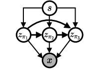
We introduce a latent variable ${\mathbf{s}}\in\mathbb{R}^{s}$ to serve as a hierarchical prior on the slots and that summarizes global statistics such as higher-order correlations between objects. This gives the following joint distribution: $p({\mathbf{x}},{\mathbf{z}}_{\pi_{1:K}},{\mathbf{s}})$, where $\pi_{1:K}:=\pi_{1},\pi_{2},\dots,\pi_{K}$ is some permutation of the integers $\{1,\dots,K\}$. We use this notation to make slot order explicit. In what follows, $\theta$ are neural net parameters for prior distributions and $\psi,\phi$ are neural net parameters for variational posterior distributions. Following common practice all latents are Gaussian with diagonal covariance.

To factorize the joint distribution over variables, we use a two-level hierarchy (Figure 1). The image ${\mathbf{x}}$, when conditioned on the slots, is independent of the scene variable:

$$p_{\theta}({\mathbf{x}},{\mathbf{z}}_{\pi_{1:K}},{\mathbf{s}})=p({\mathbf{s}})p_{\theta}({\mathbf{z}}_{\pi_{1:K}}\mid{\mathbf{s}})p_{\theta}({\mathbf{x}}\mid{\mathbf{z}}_{\pi_{1:K}}).$$ (1)

We assume a standard Gaussian for $p({\mathbf{s}})$ throughout. The slot prior is autoregressive with order $\pi_{1:K}$:

$$p_{\theta}({\mathbf{z}}_{\pi_{1:K}}\mid{\mathbf{s}})=p_{\theta}({\mathbf{z}}_{\pi_{1}}\mid{\mathbf{s}})\prod_{k=2}^{K}p_{\theta}({\mathbf{z}}_{\pi_{k}}\mid{\mathbf{z}}_{\pi_{1:k-1}},{\bm{s}}).$$ (2)

Unlike the autoregressive slot prior used by GEN and GENv2, the slot prior is conditioned on ${\mathbf{s}}$ which increases its expressiveness for modeling higher-order correlations. The conditional image likelihood can be a Gaussian:

$$p_{\theta}({\mathbf{x}}\mid{\mathbf{z}}_{\pi_{1:K}}):=\prod_{i=1}^{N}\mathcal{N}\left(\sum_{k=1}^{K}m_{i,k}x_{i,k},\sigma^{2}\right),$$ (3)

or Mixture-of-Gaussians:

$$p_{\theta}({\mathbf{x}}\mid{\mathbf{z}}_{\pi_{1:K}}):=\prod_{i=1}^{N}\sum_{k=1}^{K}m_{i,k}\mathcal{N}(x_{i,k},\sigma^{2}),$$ (4)

where $x_{i,k}\in\mathbb{R}^{C}$ is an RGB pixel, $m_{i,k}\in[0,1]$ is a mask, and $\sigma^{2}$ is a variance shared across pixels and slots. While a Gaussian likelihood is easier to optimize, the Mixture-of-Gaussians is more expressive and hence can achieve better segmentation and reconstruction quality (Burgess et al., 2019; Greff et al., 2019; Engelcke et al., 2020, 2021). We consider both in our experiments. To facilitate comparisons with previous work, we use the same spatial broadcasting decoder (SBD) (Watters et al., 2019b; Emami et al., 2021; Engelcke et al., 2021) to map slots to mixture components, and leave the exploration of alternative autoregressive decoders for future work (Singh et al., 2022). The autoregressive prior $p_{\theta}({\mathbf{z}}_{\pi_{1:K}}\mid{\mathbf{s}})$ is implemented with an LSTM (Hochreiter and Schmidhuber, 1997). To compute the input for the first slot prior $p_{\theta}({\mathbf{z}}_{\pi_{1}}\mid{\mathbf{s}})$, we project the scene variable to dimension $z$ via ${\bm{W}}_{s}^{\intercal}{\mathbf{s}}$, ${\bm{W}}_{s}\in\mathbb{R}^{s\times z}$ followed by a nonlinear activation function. Two shared linear layers are used to map the $K$ LSTM outputs to Gaussian means and variances.

To generate an image, we first sample from the scene prior and then sample sequentially from the autoregressive slot prior. The $K$ sampled slots are passed to the SBD to predict masks and RGB images. The $K$ masks are normalized with a softmax before the sum aggregation in Eq. 3 or Eq. 4.

Figure 2: Segregate, Relate, Imagine (SRI) Inference. To improve the ability of slot VAEs to learn correlations between objects, we propose learning a consistent object order for inference and generation. Inference begins by segregating the observation ${\mathbf{x}}$ to obtain randomly ordered slots ${\mathbf{z}}_{o_{1:K}}$. Next, an order-invariant relational embedding of this set is encoded into a global posterior $q_{\phi}({\mathbf{s}}\mid{\mathbf{x}})$. Finally, an imagination rollout conditioned on a sample ${\mathbf{s}}$ gives us slots with consistent order $\pi_{1:K}$. We extract order $\hat{\pi}_{1:K}$ by matching the randomly ordered and imagined slots, then transform the segregation posterior into an autoregressive posterior with order $\hat{\pi}_{1:K}$ by predicting correlated variances $\bar{\sigma}_{\hat{\pi}_{1:K}}$. The autoregressive slots ${\mathbf{z}}_{\hat{\pi}_{1:K}}$ are decoded into RGB images and masks.

4 Segregate, Relate, Imagine (SRI) Inference

In this section, we describe how to infer the latent variables in the hierarchical slot VAE introduced in Section 3. Without a canonical object order, there is no a priori order to use for slot inference, which makes inference difficult. We now introduce our inference algorithm which addresses this difficulty. Inspired by the “order matters” principle (Vinyals et al., 2016), we cast autoregressive slot inference as a set-to-sequence modeling problem, where the slot inference order is aligned to match the order in which objects are generated.

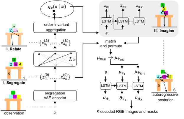
Our inference algorithm has three stages (Figure 2, Algorithm 2 in the appendix). In the first stage (Segregate, Section 4.1), we segregate the observation and obtain a randomly ordered slot posterior. In the second stage (Relate, Section 4.1), we compute order-invariant correlations between slots, which get summarized in a scene-level latent space. The third stage (Imagine, Section 4.2) transforms the segregation slot posterior into an autoregressive posterior using a learned object order.

At this point, it is reasonable to ask whether a simpler alternative to our three-stage inference algorithm could suffice, such as one based on Slot Attention (Locatello et al., 2020) with a fixed left-to-right slot order. Slot Attention is a general mechanism for grouping image pixels into slots by applying recurrent key-value-attention-based updates to a set of slots. However, in practice, imposing a fixed order on how objects are assigned to slots is surprisingly difficult. We can try to achieve this by learning $K$ distinct slot initialization parameters end-to-end (somewhat similar to SloTTAr (Gopalakrishnan et al., 2023)). However, it is unlikely that modifying Slot Attention to learn separate slot initialization parameters is sufficient for learning a fixed object inference and generation order. This would likely also require imposing an artificial ordering on the segregation step itself (e.g., always assign the bottom-most block of the block tower to slot 1), which seems non-trivial to do and is exactly what our three-stage inference algorithm avoids. As a sanity check, we compare our inference approach to a baseline that uses a modified Slot Attention encoder in Section 5.2.

4.1 Segregate, Relate

First Stage (Segregate): The segregation slot posterior is $q_{\psi}({\mathbf{z}}_{o_{1:K}}\mid{\mathbf{x}})=\prod_{k=1}^{K}q_{\psi}({\mathbf{z}}_{o_{k}}\mid{\mathbf{x}})$ with random order $o_{1:K}$. This posterior assumes slots are independent. Any appropriate existing approach can be used here (e.g., GENv2 or EMORL—non-exhaustive list, details can be found in their respective papers).

Second Stage (Relate): We use methods from set representation learning (Vaswani et al., 2017; Zaheer et al., 2017) to compute correlations between slots ${\mathbf{z}}_{o_{1:K}}$ and to encode this set for the scene posterior $q_{\phi}({\mathbf{s}}\mid{\mathbf{x}})$. This posterior summarizes order-invariant object correlations. We factorize $q_{\phi}({\mathbf{s}}\mid{\mathbf{x}})$ as a product of two simpler distributions:

$$q_{\phi}({\mathbf{s}}\mid{\mathbf{x}})=\int q_{\phi}({\mathbf{s}}\mid f_{\phi}({\mathbf{z}}_{o_{1:K}}))q_{\psi}({\mathbf{z}}_{o_{1:K}}\mid{\mathbf{x}})d{\mathbf{z}}_{o_{1:K}}.$$ (5)

Unlike GNM, which directly infers $q_{\phi}({\mathbf{s}}\mid{\mathbf{x}})$, we use the slots as a latent bottleneck to factorize $q_{\phi}({\mathbf{s}}\mid{\mathbf{x}})$. Therefore, we interpret ${\mathbf{s}}$ as a summary of the slots and their correlations. We use a single sample ${\mathbf{z}}_{o_{1:K}}$ to approximate this integral. To compute $q_{\phi}({\mathbf{s}}\mid f_{\phi}({\mathbf{z}}_{o_{1:K}}))$, we use a permutation-invariant neural network $f_{\phi}$ that estimates a relational embedding for ${\mathbf{z}}_{o_{1:K}}$. From this embedding, we compute the posterior mean and variance with two linear layers. There are many ways to implement $f_{\phi}$—we process the slots with $L$ set embedding layers followed by a permutation-invariant DeepSets (Zaheer et al., 2017) MLP with sum pooling aggregation. Each set embedding layer is implemented as residual set self-attention (Vaswani et al., 2017). To preserve the order-invariance of the segregation posterior, we remove the positional encodings and share weights across slots.

4.2 Imagining the Slot Order

Figure 3: Slot order alignment. Imagined scenes are trained to closely resemble the input scene. For example, both scenes have three objects and similar camera poses. This allows a meaningful matching between the segregation slots and imagined slots to be computed. The matching extracts the slot order to use for autoregressive inference.

So far, we have described the first two stages of SRI—first, for inferring a (randomly ordered) segregation posterior $q_{\psi}({\mathbf{z}}_{o_{1:K}}\mid{\mathbf{x}})$, and second, for inferring the scene posterior $q_{\phi}({\mathbf{s}}\mid{\mathbf{x}})$. In the third stage, we must obtain an object order to transform the (randomly ordered) segregation slot posterior into an autoregressive posterior. We extract the learned order from a slot prior rollout. Section 4.3 describes a loss for training the slot prior to learn a consistent object generation order.

Third Stage (Imagine): To obtain the slot order for inference, we first perform a scene-conditional imagination rollout to sample slots in order $\pi_{1:K}$:

$${\mathbf{s}}\sim q_{\phi}({\mathbf{s}}\mid{\mathbf{x}}),\hskip 10.00002pt{\mathbf{z}}_{\pi_{1}},\dots,{\mathbf{z}}_{\pi_{K}}\sim p_{\theta}({\mathbf{z}}_{\pi_{1}}\mid{\mathbf{s}}),\dots,p_{\theta}({\mathbf{z}}_{\pi_{K}}\mid{\mathbf{z}}_{\pi_{1:K-1}},{\mathbf{s}}).$$ (6)

We then extract the object order from ${\mathbf{z}}_{\pi_{1:K}}$ by solving for a matching between these slots and the randomly ordered segregation slots. If the imagined scene is visually similar to the input, our intuition is that the imagined order will be a suitable order for inference on the input. To encourage this similarity, we condition the rollout on the inferred scene variable (Figure 3).

Extracting the order from the imagination rollout can be done efficiently with an $O(K)$ greedy matching (Appendix Algorithm 1) that iteratively finds the best match for each slot in the rollout. Alternatively, one could use the costlier Hungarian algorithm (Munkres, 1957). Since a perfect alignment between the two sets is not guaranteed when using greedy matching, we use the notation $\hat{\pi}_{1:K}$ for the order obtained by permuting $o_{1:K}$ based on the matching. We impose $\hat{\pi}_{1:K}$ on the randomly ordered posterior by permuting the posterior means, $\mu_{o_{1:K}}\rightarrow\mu_{\hat{\pi}_{1:K}}$, and predicting new correlated variances $\bar{\sigma}^{2}_{\hat{\pi}_{1:K}}$ based on the order. The variances $\bar{\sigma}^{2}_{\hat{\pi}_{1:K}}=\texttt{LSTM}([{\bm{W}}_{s}^{\intercal}{\mathbf{s}},\mu_{\hat{\pi}_{1}},\dots,\mu_{\hat{\pi}_{K-1}}])$ are a function of the (projected) global variable ${\bm{W}}_{s}^{\intercal}{\mathbf{s}}$ and $\mu_{\hat{\pi}_{1:K-1}}$. We do not update the permuted segregation posterior means $\mu_{\hat{\pi}_{1:K}}$ and only update the variances, which we find sufficient. The scene-conditional autoregressive slot posterior is

$$q_{\phi}({\mathbf{z}}_{\hat{\pi}_{1:K}}\mid{\mathbf{s}},{\mathbf{x}})=q_{\phi}({\mathbf{z}}_{\hat{\pi}_{1}}\mid{\mathbf{s}},{\mathbf{x}})\prod_{k=2}^{K}q_{\phi}({\mathbf{z}}_{\hat{\pi}_{k}}\mid{\mathbf{z}}_{\hat{\pi}_{1:k-1}},{\mathbf{s}},{\mathbf{x}}):=\prod_{k=1}^{K}\mathcal{N}(\mu_{\hat{\pi}_{k}},\bar{\sigma}^{2}_{\hat{\pi}_{k}}).$$ (7)

To preserve order-invariance in the first two stages, we prevent gradients from flowing back through $\mu_{o_{1:K}}$ and ${\mathbf{z}}_{o_{1:K}}$.

4.3 Training Losses

We first introduce the auxiliary loss for training the slot prior to learn a consistent object generation order. This loss is combined with a variational objective for training our hierarchical slot VAE. The auxiliary loss is a reverse Kullback-Leibler (KL) divergence between the imagination rollout with order $\pi_{1:K}$ and autoregressive posterior with order $\hat{\pi}_{1:K}$. Explicitly pushing the $K$-step rollout distribution $p_{\theta}({\mathbf{z}}_{\pi_{1:K}}\mid{\mathbf{s}})$ towards the transformed slot posterior trains the prior to rollout high quality scenes; consequentially, the prior learns to adopt a consistent generation order. This loss also trains $f_{\phi}$ to extract correlations between slots ${\mathbf{z}}_{o_{1:K}}$. Intuitively, if the imagined scene resembles the input scene, the scene variable ${\mathbf{s}}$ accurately captures correlations between objects in the input scene. This “cross order” KL loss is

$$\mathcal{L}_{\text{crossOrderKL}}=\mathbb{E}_{q_{\phi}({\mathbf{s}}\mid{\mathbf{x}})}\left[D_{KL}\big{(}q_{\phi}({\mathbf{z}}_{\hat{\pi}_{1}}\mid{\mathbf{s}},{\mathbf{x}})\;\|\;p_{\theta}({\mathbf{z}}_{\pi_{1}}\mid{\mathbf{s}})\big{)}\right]$$ (8)

$$+\mathbb{E}_{q_{\phi}({\mathbf{s}}\mid{\mathbf{x}})}\Biggl{[}\sum_{k=2}^{K}\mathbb{E}_{q_{\phi}({\mathbf{z}}_{\hat{\pi}_{1:k-1}}\mid{\mathbf{s}},{\mathbf{x}})}\Bigl{[}\mathbb{E}_{{p_{\theta}({\mathbf{z}}_{\pi_{1:k-1}}\mid{\mathbf{s}})}}\bigl{[}D_{KL}\big{(}{\underbrace{q_{\phi}({\mathbf{z}}_{\hat{\pi}_{k}}\mid\star)}_{\text{Order $\hat{\pi}_{1:K}$}}}\;\|\;{\underbrace{p_{\theta}({\mathbf{z}}_{\pi_{k}}\mid\star)}_{\text{Order $\pi_{1:K}$}}}\big{)}\bigr{]}\Bigr{]}\Biggr{]},$$

where the symbol $\star$ is replaced as $q_{\phi}({\mathbf{z}}_{\hat{\pi}_{k}}\mid\star):=q_{\phi}({\mathbf{z}}_{\hat{\pi}_{k}}\mid{\mathbf{z}}_{\hat{\pi}_{1:k-1}},{\mathbf{s}},{\mathbf{x}})$ and as $p_{\theta}({\mathbf{z}}_{\pi_{k}}\mid\star):=p_{\theta}({\mathbf{z}}_{\pi_{k}}\mid{\mathbf{z}}_{\pi_{1:k-1}},{\mathbf{s}})$.

The negative ELBO objective for our hierarchical slot VAE is given by the sum of the following terms. First, we have a negative log-likelihood (reconstruction error) term:

$$\mathcal{L}_{\text{NLL}}=-\mathbb{E}_{q_{\phi}({\mathbf{s}}\mid{\mathbf{x}})}\left[\mathbb{E}_{q_{\phi}({\mathbf{z}}_{\hat{\pi}_{1:K}}\mid{\mathbf{s}},{\mathbf{x}})}\left[\log p_{\theta}({\mathbf{x}}\mid{\mathbf{z}}_{\hat{\pi}_{1:K}})\right]\right].$$ (9)

Next is a scene-level KL term:

$$\mathcal{L}_{\text{sceneKL}}=D_{KL}\big{(}q_{\phi}({\mathbf{s}}\mid{\mathbf{x}})\;\|\;p({\mathbf{s}})\big{)}.$$ (10)

The slot-level reverse KL term $\mathcal{L}_{\text{slotKL}}$ resembles $\mathcal{L}_{\text{crossOrderKL}}$ except the inner expectation is taken with respect to the slot posterior with order $\hat{\pi}_{1:K}$.

See the appendix for the full derivation. Overall, we minimize $\mathcal{L}$, the sum of the objectives for the segregation VAE ($\mathcal{L}_{\text{seg}}$) used in the Segregate stage and the SRI losses:

$$\mathcal{L}_{\text{SRI}} =\mathcal{L}_{\text{NLL}}+\mathcal{L}_{\text{sceneKL}}+\mathcal{L}_{\text{slotKL}}+\mathcal{L}_{\text{crossOrderKL}}$$ (11)

$$\mathcal{L} =\mathcal{L}_{\text{seg}}+\mathcal{L}_{\text{SRI}}.$$ (12)

We use the objective $\mathcal{L}_{\text{seg}}$ as defined by the segregation VAE. Similar to previous models (Emami et al., 2021; Engelcke et al., 2021) we dynamically balance NLL and KL with GECO (Rezende and Viola, 2018). For simplicity, we use the same SBD decoder for $\mathcal{L}_{\text{seg}}$ and $\mathcal{L}_{\text{SRI}}$.

5 Experiments

In this section we measure improvements in generation quality and correlation learning due to the scene-level variable and SRI inference. Notably, we do not expect to see changes in segmentation quality. Section 5.1 qualitatively examines sample quality and the learned order, and Sections 5.2 and 5.3 quantitatively compares against key baselines. We conduct ablation studies in Section 5.4. In the supplementary material we provide videos of random walks in the scene-level latent space to visualize higher-order object relationship learning. Throughout, we use “SRI” to refer to the entire hierarchical slot VAE trained with SRI inference.

Datasets: We use three synthetic multi-object datasets to evaluate SRI: Objects Room and CLEVR6 from the standard Multi-Object Dataset (Kabra et al., 2019) and ShapeStacks (Groth et al., 2018). All three datasets consist of rendered images of 3D scenes containing 2-6 objects and have variable illumination, shadow, and camera perspectives. Generating scenes from these datasets requires reasoning about non-trivial correlations between objects (e.g., occlusion in CLEVR6, objects resting on the floor in Objects Room, block towers in ShapeStacks).

Setup: On all datasets we train SRI with GENv2 as the segregation VAE using both Gaussian (SRI-G) and Mixture-of-Gaussians (SRI-MoG) likelihoods. On CLEVR6 we also trained SRI with EMORL. We fix $|{\mathbf{z}}_{k}|=64$, $|{\mathbf{s}}|=128$, and $L=3$ across environments. Following standard practice, on CLEVR6 and Objects Room $K=7$ and on ShapeStacks $K=9$. Remaining details for architectures, hyperparameters, and compute are in the appendix.

Baselines: We compare against state-of-the-art slot VAEs for scene generation GEN and GENv2, as well as an independent prior baseline EMORL. Results for GEN and GENv2 (GENv2-MoG) are taken from Engelcke et al. (2021) (both use the Mixture-of-Gaussians by default). GEN and GENv2-MoG results were missing for CLEVR6 so we trained these ourselves with official code releases. We train GENv2 with the Gaussian likelihood (GENv2-G) on all three datasets to directly compare with SRI-G. EMORL is trained using the official code release.

5.1 Qualitative Evaluation

(a) SRI-MoG

(b) SRI-G

(c) SRI-G*

(d) GENESISv2-G

Figure 4: ShapeStacks object generation order. Slot number indicated by mask color (legend provided: Figure 7). Best viewed in color. a) SRI learns to generate objects in a consistent order. For this training run, the model uses slot 1 for the background and slots 4-9 for blocks (most towers have only 2-4 blocks). b) SRI-G uses slots 1 and 5 for background and 6-9 for blocks (occasionally 3-4). c) SRI-G* does not use the cross-order KL term $\mathcal{L}_{\text{crossOrderKL}}$. Objects are generated in random order with slots 5-9, which can be seen by the inconsistent use of mask colors. d) GENv2-G fails to learn a consistent order which hinders learning correlations. Viz. for Objects Room and CLEVR6 are in Figure 9.

Figure 5: Randomly generated scenes. Samples from SRI-MoG and GENv2-MoG are outlined in black. Best viewed zoomed in and in color.

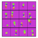
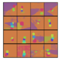
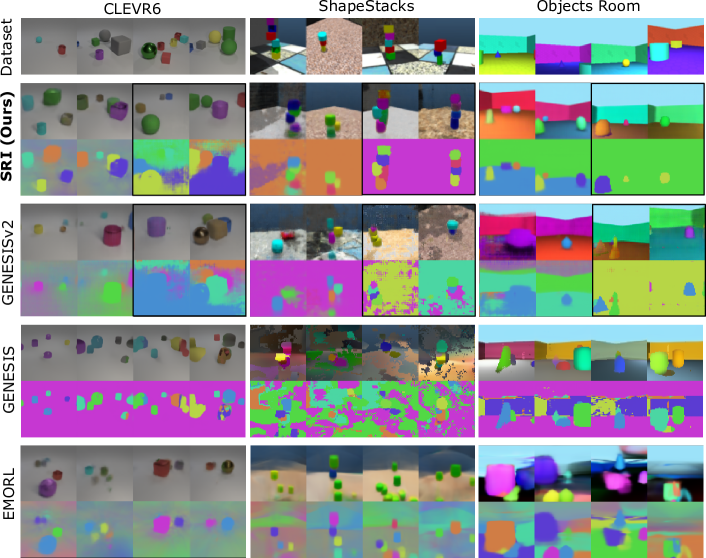
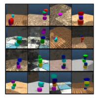
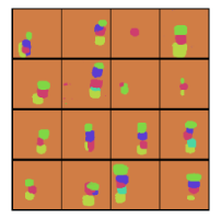
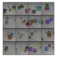
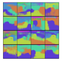
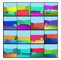
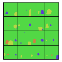
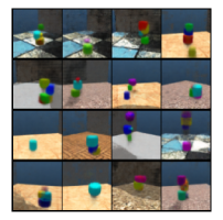
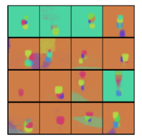
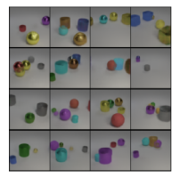
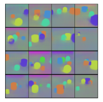
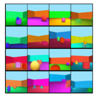
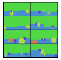
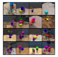
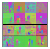
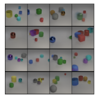
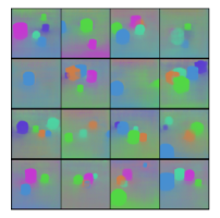
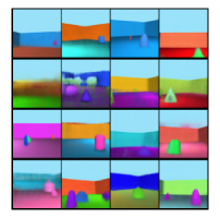
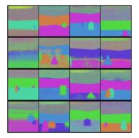
We show that SRI learns a consistent generation order by visualizing segmentation masks for randomly generated ShapeStacks scenes (Figure 4). By contrast, GENv2 fails to learn a consistent order (Figure 4(d)). Random scenes sampled from each generative model are shown in Figure 5 with additional samples in the appendix (Figures 9, 10). Across environments, SRI generates higher quality scenes than GEN, GENv2, and EMORL (Figure 5). GENv2’s samples contain artifacts and structural inaccuracies (e.g., extra walls floors in Objects Room and floating blocks in ShapeStacks). In Objects Room, GENv2-G segments the walls, floor, and sky across multiple slots, yet demonstrates a limited ability to learn the spatial correlation between these parts of the scene. GENv2-MoG fares better on Objects Room because it segments the background into a single slot. GEN’s sequential attention occasionally settles on a semi-consistent order (e.g., placing the background in the first slot for CLEVR6 and Objects Room) but in general the learned order is arbitrary and its attention mechanism fails on challenging scenes (e.g., by trying to segment ShapeStacks scenes based on color). Due to its independent slot prior, EMORL generates incoherent scenes. See Appendix A.5 for extra visualizations of random samples, test time generation with different numbers of slots, imagination rollouts, scene reconstructions, and scene segmentations.

5.2 Comparison with Learned Slot Initialization

Table 1: SRI-SA* Results. Mean $\pm$ std. dev. over 3 Shapestacks runs. All results for SRI-SA* are shown due to the high variance across random seeds.

Model FID$\downarrow$ ARI-FG$\uparrow$ -ELBO (bpd)$\downarrow$ SRI-SA* $146.3_{\tiny{\pm 83}}^{[79/97/263]}$ $0.412_{\tiny{\pm 0.316}}^{[0.82/0.36/0.05]}$ $0.940_{\tiny{\pm 0.162}}^{[0.823/0.826/1.17]}$ SRI 71.0$\pm 3$ 0.78$\pm 0.02$ 0.829$\pm 0.001$

In this section, we introduce SRI-SA*, a hierarchical autoregressive slot VAE with a modified Slot-Attention-based encoder (loosely inspired by SloTTAr (Gopalakrishnan et al., 2023) and compare it with SRI. SRI-SA* tries to learn a left-to-right ordered segregation posterior $q_{\psi}({\mathbf{z}}_{\pi_{1:K}}\mid{\mathbf{x}})$ implemented by a modified Slot Attention module. To encourage a left-to-right ordering on the slots during inference, we replace the standard Normal slot initialization in Slot Attention with learnable mean and variance parameters per slot $(\mu_{1:K},\sigma_{1:K}^{2})$. This pushes each slot to learn to specialize to a certain object in each image. While this is likely insufficient to guarantee that a stable assignment of objects to slots will be learned, we implement this approach as a simple baseline for comparison. We map each slot to a mean and variance with a linear layer during inference. All else about the SRI-SA* model is the same as SRI-MoG and we train SRI-SA* using $\mathcal{L}_{SRI}$ (Equation 11) without $\mathcal{L}_{\text{crossOrderKL}}$.

Figure 6: SRI-SA* qualitative results. We show two randomly generated scenes for each of the three models (each trained with a different random seed) and annotate them with the model’s FID score. The best model (left) learns a consistent object ordering as indicated by the consistent use of colors for the background and foreground objects unlike the second best model (middle). We observe that all models try to use all slots for each image which causes oversegmentation. Order learning and generation quality is less stable across seeds and worse overall than SRI, which we attribute to the simplistic modified Slot Attention encoder.

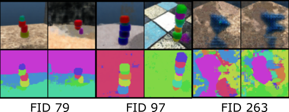
The quantitative results are shown in Table 1 and visualizations are in Figure 6. Across random seeds, SRI outperforms SRI-SA* on all metrics and qualitatively. SRI-SA* fails to consistently learn a good segregation strategy for ShapeStacks across seeds. However, the best SRI-SA* model nearly matches the average performance of SRI. This suggests that a more advanced fixed order inference approach could be a competitive alternative to our three-stage inference approach.

5.3 Quantitative Evaluation

Table 2: Main quantitative results. Mean $\pm$ std. dev. over 3 training runs. Results* are from Table 3 in Engelcke et al. (2021).

CLEVR6 Objects Room ShapeStacks Model FID$\downarrow$ ARI-FG$\uparrow$ FID$\downarrow$ ARI-FG$\uparrow$ FID$\downarrow$ ARI-FG$\uparrow$ S-Acc (%)$\uparrow$ EMORL 244.0$\pm 19$ 0.96$\pm 0.02$ 178.3$\pm 27$ 0.47$\pm 0.22$ 258.4$\pm 57$ 0.60$\pm 0.04$ - GEN 116.9$\pm 4$ 0.82$\pm 0.07$ 62.8*$\pm 3$ 0.63*$\pm 0.03$ 186.8*$\pm 18$ 0.70*$\pm 0.05$ - GENv2-G 61.0$\pm 3$ 0.98$\pm 0.00$ 87.6$\pm 4$ 0.75$\pm 0.02$ 115.3$\pm 6$ 0.68$\pm 0.02$ 50.7$\pm 3.1$ SRI-G 60.6$\pm 8$ 0.96$\pm 0.02$ 55.7$\pm 4$ 0.74$\pm 0.01$ 74.7$\pm 5$ 0.70$\pm 0.01$ 72.0$\pm 3.5$ GENv2-MoG 61.0$\pm 3$ 0.98$\pm 0.00$ 52.6*$\pm 3$ 0.85*$\pm 0.01$ 112.7*$\pm 3$ 0.81*$\pm 0.00$ 59 SRI-MoG 54.4$\pm 2$ 0.97$\pm 0.01$ 48.4$\pm 4$ 0.83$\pm 0.02$ 70.4$\pm 3$ 0.78$\pm 0.02$ 80.7$\pm 5.0$

Table 3: SRI ablations. SRI-G on ShapeStacks, mean $\pm$ std. dev. over 3 runs. The negative ELBO in bits-per-dim (bpd) is a single sample Monte Carlo estimate averaged over 5k validation scenes.

Learned order Scene variable $\mathcal{L}_{\text{crossOrderKL}}$ FID$\downarrow$ $\mathcal{L}_{\text{SRI}}$(bpd)$\downarrow$ S-Acc (%)$\uparrow$ a) ✓ ✓ 132.9$\pm 2$ (-57.9) 0.836$\pm 0.001$ 31.7$\pm 6.4$ b) ✓ - 123.2$\pm 3$ (-48.2) 0.845$\pm 0.001$ 43.7$\pm 10.7$ c) ✓ ✓ 106.3$\pm 3$ (-31.3) 0.833$\pm 0.001$ 61.3$\pm 1.5$ d) ✓ ✓ ✓ 75.0$\pm 6$ (+0.0) 0.829$\pm 0.001$ 72.0$\pm 3.5$

Table 4: Scene variable ablation. Mean $\pm$ std. dev. over 3 Shapestacks runs except for results^∗ computed with model weights released by the authors. The negative ELBO in bits-per-dim (bpd) is a single sample Monte Carlo estimate averaged over 5k validation scenes.

Model FID$\downarrow$ -ELBO (bpd)$\downarrow$ S-Acc (%)$\uparrow$ GEN^∗ 233.3 0.832 - GEN + scene variable 217.5$\pm 22$ 1.051$\pm 0.120$ - GENv2^∗ 107.4 0.821 59 GENv2 + scene variable 84.5$\pm 4$ 0.823$\pm 0.000$ 66.3$\pm 10.7$ SRI 71.0$\pm 3$ 0.829$\pm 0.001$ 80.7$\pm 5.0$

We use the Fréchet Inception Distance (FID) (Heusel et al., 2017) to quantify the visual similarity of generated scenes to training scenes. Inspired by the evaluation in GNM (Jiang and Ahn, 2020), we measure the ability to learn higher-order correlations by manually labeling 100 ShapeStacks scenes generated by each model and computing the percent of scenes that contain a physically plausible stack of blocks, i.e., all blocks in the stack are touching each other (structural accuracy, or S-Acc). We use officially released model weights to compute S-Acc for GEN and GENv2-MoG. Following standard practice for evaluating segregation quality we use the adjusted rand index (Rand, 1971; Hubert and Arabie, 1985) for foreground objects only (ARI-FG).

Results are in Table 2. Out of the slot VAEs, SRI achieves the lowest FID scores on all environments and the best S-Acc score. SRI-G improves GENv2-G’s FID by an average of 24% and SRI-MoG improves GENv2-MoG’s FID by an average of 19%. On CLEVR6, we observe that SRI achieves the smallest improvement in FID over GENv2, which we believe is caused by a) CLEVR6 only having simple correlations to learn (e.g., occlusion) and b) small artifacts introduced by GENv2’s encoder which seems to negatively impact the FID score on this dataset. GENv2-G segregates the walls, floor, and sky into different slots on Objects Room which makes correlation learning difficult, leading to a poor FID score and which SRI-G improves by 36%. In general, we find that the segregation quality of SRI closely matches that of the slot VAE used for scene segregation, and that better ARI-FG correlates with better sample quality for SRI.

To demonstrate the flexibility of SRI, we also train SRI using EMORL to extract randomly ordered slots on CLEVR6. We see a significant improvement in FID from EMORL to SRI-EMORL (244$\pm 19$ to 48.9$\pm 7$, also see Figure 14).

5.4 Ablation Studies

We now examine each contribution individually with ShapeStacks’s validation set.

Scene-level variable: First, we isolate the scene-level variable by adding a scene-level variable to GEN and GENv2, leaving all else with these models the same. For scene-level inference with GEN, we encode the ordered sequence of slots obtained by sampling from its ordered slot posterior. Scene-level inference for GENv2 is the same as with SRI. Results are in Table 4. Augmenting GEN with a scene variable does little to improve its performance since it still fails to properly segregate ShapeStacks scenes. GENv2 enjoys a moderate improvement in FID score and S-Acc but does not match the performance of SRI—the latter which has the combined benefit of both the scene variable and of using a consistent object order. The higher negative ELBO values for SRI are due to the additional KL terms. These results suggest the scene variable alone does not account for all of SRI’s demonstrated performance improvements.

SRI Inference: Next, we ablate the core aspects of SRI inference using the SRI-G model (Table 3). a) We remove the scene-level variable. The prior for SRI’s first slot becomes $p({\mathbf{z}}_{1}):=\mathcal{N}(0,1)$. Without a scene-level variable, sample quality is significantly worse. SRI inference no longer works properly; the imagination rollout is now unconditional and imagined scenes are not similar to the input ${\mathbf{x}}$. The model fails to learn a consistent generation order to align the slot segregation posterior to. b) We ablate the order alignment step of SRI inference. That is, during inference we never transform the first stage slot posterior with random slot order $o_{1:K}$ into an autoregressive posterior with imagined order $\hat{\pi}_{1:K}$ (we also therefore remove $\mathcal{L}_{\text{crossOrderKL}}$ from the loss). SRI with a randomly ordered slot posterior has difficulty learning object correlations and the sample quality is poor. c) If we only remove $\mathcal{L}_{\text{crossOrderKL}}$, SRI’s prior fails to learn a consistent order and correlation estimation suffers. This results in a significant drop in sample quality (see Figure 4(c)). Overall, we find that the scene-level variable, order alignment, and auxiliary loss all play a critical role for SRI inference.

6 Conclusion

In this work we demonstrated strategies for improving the ability of autoregressive slot VAEs to learn multi-object correlations, which resulted in gains in scene generation quality. To achieve this, we proposed augmenting slots with a scene-level latent variable and learning a consistent object order. These improvements are agnostic to the choice of model that initially extracts the slots from images. Recently, it was shown that frozen image encoders pretrained with self-supervised learning greatly improve the robustness of slot-based models, particularly on real world scenes (Seitzer et al., 2023). We believe exploring the use of frozen encoders with SRI is a promising direction.

One limitation of SRI inference is that it does not learn causal relations between objects but rather only correlations, which only weakly generalize outside the training distribution (Schölkopf et al., 2021). Extending SRI to dynamic settings would enable exploring causal inference of dependencies. Another limitation of SRI is it requires solving a computationally demanding matching problem during inference. We suggest a linear-time approximate matching algorithm in this work, but this may scale poorly to more complex environments. Finally, there appears to be only limited benefits to learning an object ordering for environments such as CLEVR6 where scenes have little structure and objects are only weakly correlated. However, learning an order does not seem to hurt performance in this situation.

There are not immediate negative societal implications of this work. However, future work on deep generative modeling that builds on our ideas could plausibly cause harm. Research on mitigation strategies for these scenarios is ongoing (Mishkin et al., 2022).

Acknowledgments

We thank Dave Biagioni and Peter Graf for providing valuable comments and suggested revisions. Patrick Emami was supported in parts by the Florida DOT under grant BDV31 977-116, an FEF McKnight fellowship, and the National Renewable Energy Laboratory, operated by Alliance for Sustainable Energy, LLC, for the U.S. Department of Energy (DOE) under Contract No. DE-AC36-08GO28308. This work was supported by the Laboratory Directed Research and Development (LDRD) Program at NREL. The views expressed in the article do not necessarily represent the views of the DOE or the U.S. Government. The U.S. Government retains and the publisher, by accepting the article for publication, acknowledges that the U.S. Government retains a nonexclusive, paid-up, irrevocable, worldwide license to publish or reproduce the published form of this work, or allow others to do so, for U.S. Government purposes.

Appendix A Appendix

A.1 Matching Pseudocode

Algorithm 1 Greedy matching. Uses $O(K)$ time and $O(K^{2})$ space.

1:  Input: Randomly ordered segregation posterior means $\mu_{o_{1:K}}$, imagination rollout means $\mu_{\pi_{1:K}}$

2:  ${\bm{C}}[i,j]=\lVert\mu_{\pi_{i}}-\mu_{o_{j}}\rVert_{2},$   $\forall i,j=1,\dots,K$

3:  $\sigma:=\texttt{zeros}(K,K)$

4:  for index $i=0\dots K-1$ do

5:     $j^{*}=\operatorname*{arg\,min}{\bm{C}}[i,:]$

6:     ${\bm{C}}[:,j^{*}]=+\inf$

7:     $\sigma[j^{*},i]=1$

8:  end for

9:  return  Permutation $\sigma$

Alternative matching algorithms such as the Hungarian algorithm (Munkres, 1957) can be used instead at a higher computational cost; however, we leave an empirical comparison of these algorithms for future work.

A.2 SRI Inference Pseudocode

Algorithm 2 SRI Inference. All sampling uses the Gaussian reparameterization trick (Kingma and Welling, 2014).

1:  Input: Scene observation ${\mathbf{x}}$, segregation VAE encoder $e_{\psi}({\mathbf{x}})$, scene-level encoder $f_{\phi}({\mathbf{z}})$, autoregressive prior $\texttt{LSTM}_{\theta}$, autoregressive posterior $\texttt{LSTM}_{\phi}$

2:  ${\mathbf{z}}_{o_{1:K}}\sim q_{\psi}({\mathbf{z}}_{o_{1:K}}\mid{\mathbf{x}})\leftarrow e_{\psi}({\mathbf{x}})$ /* Segregate */

3:  ${\mathbf{s}}\sim q_{\phi}({\mathbf{s}}\mid{\mathbf{x}})\leftarrow f_{\phi}({\mathbf{z}}_{o_{1:K}})$ /* Relate */

4:  ${\mathbf{z}}_{\pi_{1}}\sim p_{\theta}({\mathbf{z}}_{\pi_{1}}\mid{\mathbf{s}})\leftarrow\texttt{LSTM}_{\theta}(\{{\mathbf{s}}\})$ /* Imagine */

5:  ${\mathbf{z}}_{\pi_{k}}\sim p_{\theta}({\mathbf{z}}_{\pi_{k}}\mid{\mathbf{z}}_{\pi_{1:k-1}},{\mathbf{s}})\leftarrow\texttt{LSTM}_{\theta}(\{{\mathbf{s}},{\mathbf{z}}_{\pi_{1:k-1}}\})$ for all $k=2,\dots,K-1$

6:  $\sigma\leftarrow$ Matching $({\mathbf{z}}_{o_{1:K}},{\mathbf{z}}_{\pi_{1:K}})$ /* we pass the posterior means to Algorithm 1 */

7:  $\mu_{o_{1:K}}\xrightarrow{\sigma}\mu_{\hat{\pi}_{1:K}}$ /* apply the permutation to the $K$ means of $q_{\phi}({\mathbf{z}}_{o_{1:K}}\mid{\mathbf{x}})$ */

8:  $\bar{\sigma}^{2}_{\hat{\pi}_{1}}\leftarrow\texttt{LSTM}_{\phi}(\{{\mathbf{s}}\})$ /* predict new correlated variances */

9:  $\bar{\sigma}^{2}_{\hat{\pi}_{k}}\leftarrow\texttt{LSTM}_{\phi}(\{{\mathbf{s}},\mu_{\hat{\pi}_{1:k-1}}\})$ for all $k=2,\dots,K-1$

10:  $q_{\phi}({\mathbf{z}}_{\hat{\pi}_{1:K}}\mid{\mathbf{s}},{\mathbf{x}}):=\prod_{k=1}^{K}\mathcal{N}(\mu_{\hat{\pi}_{k}},\bar{\sigma}^{2}_{\hat{\pi}_{k}})$ /* autoregressive slot posterior */

11:  return  The sufficient statistics (e.g., means and variances) for the segregation posterior $q_{\psi}({\mathbf{z}}_{o_{1:K}}\mid{\mathbf{x}})$, scene posterior $q_{\phi}({\mathbf{s}}\mid{\mathbf{x}})$, autoregressive slot posterior $q_{\phi}({\mathbf{z}}_{\hat{\pi}_{1:K}}\mid{\mathbf{s}},{\mathbf{x}})$

Our proposed inference algorithm involves aligning the object order of the segregation slot posterior to a learned object order (Lines 6-7) and then transforming this posterior into an autoregressive distribution by predicting a sequence of correlated variances (Lines 8-10).

A.3 ELBO Derivation

We derive a lower bound on the log marginal scene likelihood as follows:

$$\log p({\mathbf{x}}) =\log\int p_{\theta}({\mathbf{x}},{\mathbf{s}},{\mathbf{z}}_{\pi_{1:K}})d{\mathbf{s}},d{\mathbf{z}}_{\pi_{1:K}}$$ (13)

$$=\log\int\frac{q_{\phi}({\mathbf{s}},{\mathbf{z}}_{\pi_{1:K}}\mid{\mathbf{x}})}{q_{\phi}({\mathbf{s}},{\mathbf{z}}_{\pi_{1:K}}\mid{\mathbf{x}})}p_{\theta}({\mathbf{x}},{\mathbf{s}},{\mathbf{z}}_{\pi_{1:K}})d{\mathbf{s}},d{\mathbf{z}}_{\pi_{1:K}}$$ (14)

$$=\log\mathbb{E}_{q_{\phi}({\mathbf{s}},{\mathbf{z}}_{\pi_{1:K}}\mid{\mathbf{x}})}\left[\frac{p_{\theta}({\mathbf{x}},{\mathbf{s}},{\mathbf{z}}_{\pi_{1:K}})}{q_{\phi}({\mathbf{s}},{\mathbf{z}}_{\pi_{1:K}}\mid{\mathbf{x}})}\right].$$ (15)

Applying Jensen’s inequality and then factorizing gives:

$$\log p({\mathbf{x}}) \geq\mathbb{E}_{q_{\phi}({\mathbf{s}},{\mathbf{z}}_{\pi_{1:K}}\mid{\mathbf{x}})}\left[\log\frac{p_{\theta}({\mathbf{x}},{\mathbf{s}},{\mathbf{z}}_{\pi_{1:K}})}{q_{\phi}({\mathbf{s}},{\mathbf{z}}_{\pi_{1:K}}\mid{\mathbf{x}})}\right]$$ (16)

$$=\mathbb{E}_{q_{\phi}({\mathbf{s}}\mid{\mathbf{x}})}\left[\mathbb{E}_{q_{\phi}({\mathbf{z}}_{\pi_{1:K}}\mid{\mathbf{s}},{\mathbf{x}})}\left[\log\frac{p({\mathbf{s}})p_{\theta}({\mathbf{z}}_{\pi_{1:K}}\mid{\mathbf{s}})p_{\theta}({\mathbf{x}}\mid{\mathbf{z}}_{\pi_{1:K}})}{q_{\phi}({\mathbf{s}}\mid{\mathbf{x}})q_{\phi}({\mathbf{z}}_{\pi_{1:K}}\mid{\mathbf{s}},{\mathbf{x}})}\right]\right].$$ (17)

We use the fact that $\log(\frac{A}{B}\frac{C}{D})=\log(\frac{A}{B})+\log(\frac{C}{D})$ to factor Eq. 17 into a sum of three losses. The autoregressive slot posterior order obtained for inference $\color[rgb]{0,0,1}\definecolor[named]{pgfstrokecolor}{rgb}{0,0,1}{\hat{\pi}_{1:K}}$ is shown in blue.

The first term is a negative log-likelihood loss:

$$\mathcal{L}_{\text{NLL}}=-\mathbb{E}_{q_{\phi}({\mathbf{s}}\mid{\mathbf{x}})}\left[\mathbb{E}_{q_{\phi}({\mathbf{z}}_{\color[rgb]{0,0,1}\definecolor[named]{pgfstrokecolor}{rgb}{0,0,1}{\hat{\pi}_{1:K}}}\mid{\mathbf{s}},{\mathbf{x}})}\left[\log p_{\theta}({\mathbf{x}}\mid{\mathbf{z}}_{\color[rgb]{0,0,1}\definecolor[named]{pgfstrokecolor}{rgb}{0,0,1}{\hat{\pi}_{1:K}}})\right]\right].$$ (18)

The second is a slot-level reverse KL loss with the approximate order:

$$\mathcal{L}_{\text{slotKL}}=-\mathbb{E}_{q_{\phi}({\mathbf{s}}\mid{\mathbf{x}})}\left[\mathbb{E}_{q_{\phi}({\mathbf{z}}_{\color[rgb]{0,0,1}\definecolor[named]{pgfstrokecolor}{rgb}{0,0,1}{\hat{\pi}_{1:K}}}\mid{\mathbf{s}},{\mathbf{x}})}\left[\log\frac{p_{\theta}({\mathbf{z}}_{\color[rgb]{0,0,1}\definecolor[named]{pgfstrokecolor}{rgb}{0,0,1}{\hat{\pi}_{1:K}}}\mid{\mathbf{s}})}{q_{\phi}({\mathbf{z}}_{\color[rgb]{0,0,1}\definecolor[named]{pgfstrokecolor}{rgb}{0,0,1}{\hat{\pi}_{1:K}}}\mid{\mathbf{s}},{\mathbf{x}})}\right]\right]$$ (19)

$$=\mathbb{E}_{q_{\phi}({\mathbf{s}}\mid{\mathbf{x}})}\left[\mathbb{E}_{q_{\phi}({\mathbf{z}}_{\color[rgb]{0,0,1}\definecolor[named]{pgfstrokecolor}{rgb}{0,0,1}{\hat{\pi}_{1:K}}}\mid{\mathbf{s}},{\mathbf{x}})}\left[\log\frac{q_{\phi}({\mathbf{z}}_{\color[rgb]{0,0,1}\definecolor[named]{pgfstrokecolor}{rgb}{0,0,1}{\hat{\pi}_{1:K}}}\mid{\mathbf{s}},{\mathbf{x}})}{p_{\theta}({\mathbf{z}}_{\color[rgb]{0,0,1}\definecolor[named]{pgfstrokecolor}{rgb}{0,0,1}{\hat{\pi}_{1:K}}}\mid{\mathbf{s}})}\right]\right]$$ (20)

$$=\mathbb{E}_{q_{\phi}({\mathbf{s}}\mid{\mathbf{x}})}\left[\sum_{k=1}^{K}\mathbb{E}_{q_{\phi}({\mathbf{z}}_{\color[rgb]{0,0,1}\definecolor[named]{pgfstrokecolor}{rgb}{0,0,1}{\hat{\pi}_{1:k}}}\mid{\mathbf{s}},{\mathbf{x}})}\left[\log\frac{q_{\phi}({\mathbf{z}}_{\color[rgb]{0,0,1}\definecolor[named]{pgfstrokecolor}{rgb}{0,0,1}{\hat{\pi}_{k}}}\mid{\mathbf{z}}_{\color[rgb]{0,0,1}\definecolor[named]{pgfstrokecolor}{rgb}{0,0,1}{\hat{\pi}_{1:k-1}}},{\mathbf{s}},{\mathbf{x}})}{p_{\theta}({\mathbf{z}}_{\color[rgb]{0,0,1}\definecolor[named]{pgfstrokecolor}{rgb}{0,0,1}{\hat{\pi}_{k}}}\mid{\mathbf{z}}_{\color[rgb]{0,0,1}\definecolor[named]{pgfstrokecolor}{rgb}{0,0,1}{\hat{\pi}_{1:k-1}}},{\mathbf{s}})}\right]\right]$$ (21)

$$=\mathbb{E}_{q_{\phi}({\mathbf{s}}\mid{\mathbf{x}})}\left[D_{KL}\big{(}q_{\phi}({\mathbf{z}}_{\color[rgb]{0,0,1}\definecolor[named]{pgfstrokecolor}{rgb}{0,0,1}{\hat{\pi}_{1}}}\mid{\mathbf{s}},{\mathbf{x}})\;\|\;p_{\theta}({\mathbf{z}}_{\color[rgb]{0,0,1}\definecolor[named]{pgfstrokecolor}{rgb}{0,0,1}{\hat{\pi}_{1}}}\mid{\mathbf{s}})\big{)}\right]$$ (22)

$$\phantom{=}+\mathbb{E}_{q_{\phi}({\mathbf{s}}\mid{\mathbf{x}})}\left[\sum_{k=2}^{K}\mathbb{E}_{q_{\phi}({\mathbf{z}}_{\color[rgb]{0,0,1}\definecolor[named]{pgfstrokecolor}{rgb}{0,0,1}{\hat{\pi}_{1:k-1}}}\mid{\mathbf{s}},{\mathbf{x}})}\left[D_{KL}\big{(}q_{\phi}({\mathbf{z}}_{\color[rgb]{0,0,1}\definecolor[named]{pgfstrokecolor}{rgb}{0,0,1}{\hat{\pi}_{k}}}\mid{\mathbf{z}}_{\color[rgb]{0,0,1}\definecolor[named]{pgfstrokecolor}{rgb}{0,0,1}{\hat{\pi}_{1:k-1}}},{\mathbf{s}},{\mathbf{x}})\;\|\;p_{\theta}({\mathbf{z}}_{\color[rgb]{0,0,1}\definecolor[named]{pgfstrokecolor}{rgb}{0,0,1}{\hat{\pi}_{k}}}\mid{\mathbf{z}}_{\color[rgb]{0,0,1}\definecolor[named]{pgfstrokecolor}{rgb}{0,0,1}{\hat{\pi}_{1:k-1}}},{\mathbf{s}})\big{)}\right]\right].$$ (23)

The third term is a scene-level reverse KL loss:

$$\mathcal{L}_{\text{sceneKL}} =-\mathbb{E}_{q_{\phi}({\mathbf{s}}\mid{\mathbf{x}})}\left[\mathbb{E}_{q_{\phi}({\mathbf{z}}_{\pi_{1:K}}\mid{\mathbf{s}},{\mathbf{x}})}\left[\log\frac{p({\mathbf{s}})}{q_{\phi}({\mathbf{s}}\mid{\mathbf{x}})}\right]\right]$$ (24)

$$=-\mathbb{E}_{q_{\phi}({\mathbf{s}}\mid{\mathbf{x}})}\left[\log\frac{p({\mathbf{s}})}{q_{\phi}({\mathbf{s}}\mid{\mathbf{x}})}\right]$$ (25)

$$=\mathbb{E}_{q_{\phi}({\mathbf{s}}\mid{\mathbf{x}})}\left[\log\frac{q_{\phi}({\mathbf{s}}\mid{\mathbf{x}})}{p({\mathbf{s}})}\right]$$ (26)

$$=D_{KL}\big{(}q_{\phi}({\mathbf{s}}\mid{\mathbf{x}})\;\|\;p({\mathbf{s}})\big{)}.$$ (27)

We also define an auxiliary slot-level reverse KL loss similar to Eq. 23 except that the inner expectation is now taken with respect to the slot posterior and the $K$-step rollout with order $\pi_{1:K}$:

$$\mathcal{L}_{\text{crossOrderKL}}=\mathbb{E}_{q_{\phi}({\mathbf{s}}\mid{\mathbf{x}})}\left[D_{KL}\big{(}q_{\phi}({\mathbf{z}}_{\color[rgb]{0,0,1}\definecolor[named]{pgfstrokecolor}{rgb}{0,0,1}{\hat{\pi}_{1}}}\mid{\mathbf{s}},{\mathbf{x}})\;\|\;p_{\theta}({\mathbf{z}}_{\pi_{1}}\mid{\mathbf{s}})\big{)}\right]$$ (28)

$$\phantom{=}+\mathbb{E}_{q_{\phi}({\mathbf{s}}\mid{\mathbf{x}})}\left[\sum_{k=2}^{K}\mathbb{E}_{q_{\phi}({\mathbf{z}}_{\color[rgb]{0,0,1}\definecolor[named]{pgfstrokecolor}{rgb}{0,0,1}{\hat{\pi}_{1:k-1}}}\mid{\mathbf{s}},{\mathbf{x}})}\left[\mathbb{E}_{p_{\theta}({\mathbf{z}}_{\pi_{1:k-1}}\mid{\mathbf{s}})}\left[D_{KL}\big{(}q_{\phi}({\mathbf{z}}_{\color[rgb]{0,0,1}\definecolor[named]{pgfstrokecolor}{rgb}{0,0,1}{\hat{\pi}_{k}}}\mid\star)\;\|\;p_{\theta}({\mathbf{z}}_{\pi_{k}}\mid\star)\big{)}\right]\right]\right],$$ (29)

where $q_{\phi}({\mathbf{z}}_{\color[rgb]{0,0,1}\definecolor[named]{pgfstrokecolor}{rgb}{0,0,1}{\hat{\pi}_{k}}}\mid\star):=q_{\phi}({\mathbf{z}}_{\color[rgb]{0,0,1}\definecolor[named]{pgfstrokecolor}{rgb}{0,0,1}{\hat{\pi}_{k}}}\mid{\mathbf{z}}_{\color[rgb]{0,0,1}\definecolor[named]{pgfstrokecolor}{rgb}{0,0,1}{\hat{\pi}_{1:k-1}}},{\mathbf{s}},{\mathbf{x}})$ and $p_{\theta}({\mathbf{z}}_{\pi_{k}}\mid\star):=p_{\theta}({\mathbf{z}}_{\pi_{k}}\mid{\mathbf{z}}_{\pi_{1:k-1}},{\mathbf{s}})$. The auxiliary KL term is always non-negative by definition, so adding it to the negative ELBO only increases the upper bound on $-\log p({\mathbf{x}})$ (equivalently, loosens the lower bound on $\log p({\mathbf{x}})$). Summed together, the four terms form the SRI loss: $\mathcal{L}_{\text{SRI}}={\mathcal{L}}_{\text{NLL}}+\mathcal{L}_{\text{slotKL}}+\mathcal{L}_{\text{crossOrderKL}}+\mathcal{L}_{\text{sceneKL}}$. In practice, we approximate the expectations with a single sample and average the loss over a minibatch of size $B=32$ of dataset samples. We leave a formal characterization of how the accuracy of the matching between $\hat{\pi}$ and $\pi$ affects the lower bound on the marginal log likelihood for future work. Intuitively, as long as the two slot orders are “close”, we can expect these lower bounds to be similar as well.

A.4 Experiment details

A.4.1 Hyperparameters

Architecture: We use $|{\mathbf{z}}_{k}|=64$ for all environments following GENv2 and EMORL. We set $|{\mathbf{s}}|=128$ to be twice the slot dimension. The number of attention layers for scene posterior estimation is fixed at $L=3$; we found that varying $L$ incurred little change in performance. We use the same hyperparameters for the image encoder and decoder architectures as used by GENv2 and EMORL for SRI-G, SRI-MoG, and SRI-EMORL, respectively. Both of the GENv2 and EMORL implementations are based on open source released by the respective authors. For SRI-EMORL we fix the number of iterative refinement steps to 2. Following GEN and GENv2, SRI’s autoregressive prior and posterior LSTM uses 256 hidden units. When training GENv2 jointly with SRI we replace its autoregressive prior with a slot-wise independent prior. SRI uses GELU non-linear activations (Hendrycks and Gimpel, 2016) after each linear projection of the scene variable and in the attention layers. All layers use Xavier weight initialization (Glorot and Bengio, 2010).

In the scene encoder, each set embedding layer is defined as follows:

$$\alpha=\texttt{softmax}\Bigl{(}\frac{({\mathbf{z}}_{o_{1:K}}{\bm{W}}_{k})({\mathbf{z}}_{o_{1:K}}{\bm{W}}_{q})^{\intercal}}{\sqrt{z}}\Bigr{)},\hskip 10.00002pt\hat{{\mathbf{z}}}_{o_{i}}=\sum_{j=1}^{K}\alpha_{ij}\bigl{(}{\bm{W}}_{v}^{\intercal}[{\mathbf{z}}_{o_{j}};{\mathbf{z}}_{o_{i}}-{\mathbf{z}}_{o_{j}}]\bigr{)},$$ (30)

$${\mathbf{z}}^{\prime}_{o_{i}}={\mathbf{z}}_{o_{i}}+g_{\phi}({\mathbf{z}}_{o_{i}},{\mathbf{z}}_{o_{1:K}}),\hskip 10.00002ptg_{\phi}({\mathbf{z}}_{o_{i}},{\mathbf{z}}_{o_{1:K}}):=\texttt{MLP}(\texttt{LayerNorm}({\mathbf{z}}_{o_{i}}+\hat{{\mathbf{z}}}_{o_{1:K}}).$$ (31)

Here, ${\bm{W}}_{q},{\bm{W}}_{k}\in\mathbb{R}^{z\times z},{\bm{W}}_{v}\in\mathbb{R}^{2z\times z}$, $[;]$ is concatenation, and $\alpha$ is the $K\times K$ scaled dot-product self-attention computed with keys and queries given by linear projections of ${\mathbf{z}}_{o_{1:K}}$. To potentially create a stronger inductive bias for encoding directed dependencies, we used the difference between slots ${\mathbf{z}}_{o_{i}}-{\mathbf{z}}_{o_{j}}$ as an additional feature in Eq. 30 (Santoro et al., 2017). However, empirically we did not observe any improvements from this modification.

Optimization: We mostly adopt the same hyperparameters here as used by GENv2 and EMORL. SRI based on GENv2 uses the Adam optimizer (Kingma and Ba, 2015) with default hyperparameters and a learning rate of 1e-4 but without any learning rate schedule. SRI-EMORL uses an initial learning rate of 4e-4, grad norm clipping to 5, and learning rate schedule consisting of a linear warmup for 10K steps then multiplicative decay with by a rate of 0.5 every 100K steps. A batch size of 32 is used for all models. Both GENv2 and EMORL use GECO to balance reconstruction and KL during optimization; we discuss the GECO hyperparameters in Section A.4.2.

Datasets: Both CLEVR6 and Objects Room can be accessed freely online under the Apache License 2.0. The ShapeStacks dataset is also freely available for download online under the GNU License 3.0.. We use the same preprocessing protocol for CLEVR6 as Emami et al. (2021), which is to center crop the images to 192x192 and the resize them to size 96x96. Objects Room and ShapeStacks have 64x64 RGB images.

A.4.2 Balancing reconstruction and KL with GECO

Both GENv2 and EMORL use GECO to balance the reconstruction and KL losses (Rezende and Viola, 2018). Each code base has its own GECO implementation and GECO hyperparameter schedule which we use to train SRI-G, SRI-MoG, and SRI-EMORL.

SRI-G (unnormalized Gaussian image likelihood and global $\sigma$ = 0.7) uses a per-pixel and per-channel GECO target of -0.353 on Objects Room and ShapeStacks and -0.356 on CLEVR6. We decreased the GECO learning rate from 1e-5 to 1e-6. Once the GECO target is reached the learning rate is multiplied by a speedup factor of 10 to accelerate the decay of the GECO Lagrange parameter.

SRI-MoG uses the same GECO hyperparameters as GENv2-MoG on ShapeStacks and Objects Room (target is 0.5655—note that the MoG likelihood here is normalized) except we also use the decreased GECO learning rate of 1e-6. However, on Objects Room we notice that this increasesed training instability, likely because this warms up the KL less aggressively than the faster GECO learning rate does. We use restarting from model checkpoints to mitigate this here.

For SRI-EMORL on CLEVR6 we used a target of -2.265 for unnormalized Gaussian image likelihood with global $\sigma$ = 0.1. The rule of thumb used to tune the GECO target is that the target should be reached after about 20% of the training steps. This gives ample time for the GECO Lagrange parameter to automatically decay back to 1 so that a valid ELBO is eventually maximized. We use a GECO learning rate of 1e-6 and speedup of 10 as well.

A.4.3 Baselines and compute

GENESIS and GENESIS-v2: The authors of GENv2 have released pre-trained weights for GEN trained on ShapeStacks and GENv2-MoG trained on Objects Room and ShapeStacks. We use these weights for model visualizations and to compute the structure accuracy metric. To train GENv2-MoG on CLEVR6 we had to lower the standard deviation to 0.1. We adjusted the GENv2-MoG GECO target accordingly by tuning it to -2.265. To compute the FID score, we follow the same protocol as GENv2 (Engelcke et al., 2021) and use 10K real and generated samples.

Compute: In general, the majority of the compute is taken up by the segregation VAE (GENv2 and EMORL in this work). SRI adds a few lightweight neural networks and therefore only marginally increases training time.

• On Objects Room and ShapeStacks, SRI-X takes about 20 hours to reach 500K steps using 2 NVIDIA A100 GPUs. On CLEVR6, it about 24 hours to reach 425K steps, at which point we stopped training since the model showed signs of convergence and so as to keep training times at about one day or faster on equivalent hardware to ease reproducibility.

• The GENv2 and GEN baselines are negligibly faster to train. We train these baselines using the same setup as SRI.

• SRI-EMORL uses 8 NVIDIA A100 GPUs to reach 225K CLEVR6 which takes about 27 hours, at which point we cut off training to keep a similar compute budget to SRI with GENv2. The memory footprint of the two steps of iterative refinement used to estimate the segregation posterior is large, hence the need for 8 GPUs.

A.4.4 Open source software

This project was conducting using the following open source Python packages: PyTorch (Paszke et al., 2019), numpy (Harris et al., 2020), jupyter (Kluyver et al., 2016), matplotlib (Hunter, 2007), scikit-learn (Pedregosa et al., 2011), and sacred (Greff et al., 2017).

A.5 Additional Qualitative Results

Figure 7: Mask color to slot number legend

Figure 8: Failure cases. Examples of ShapeStacks scenes randomly sampled from SRI-MoG that are of poor quality. Floating blocks and blocks occupying the same space are hallmarks of failures.

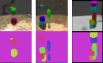
Failure cases: We show failed scene generations from SRI-MoG in Figure 8. Future directions that could help improve scene generation quality include making the model end-to-end differentiable and using a pretrained image encoder.

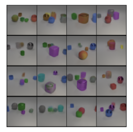
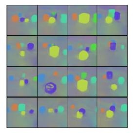
Additional random samples: We visualize extra randomly sampled scenes from SRI-MoG (Figure 9), SRI-G (Figure 10), and GENv2-G (Figure 11).

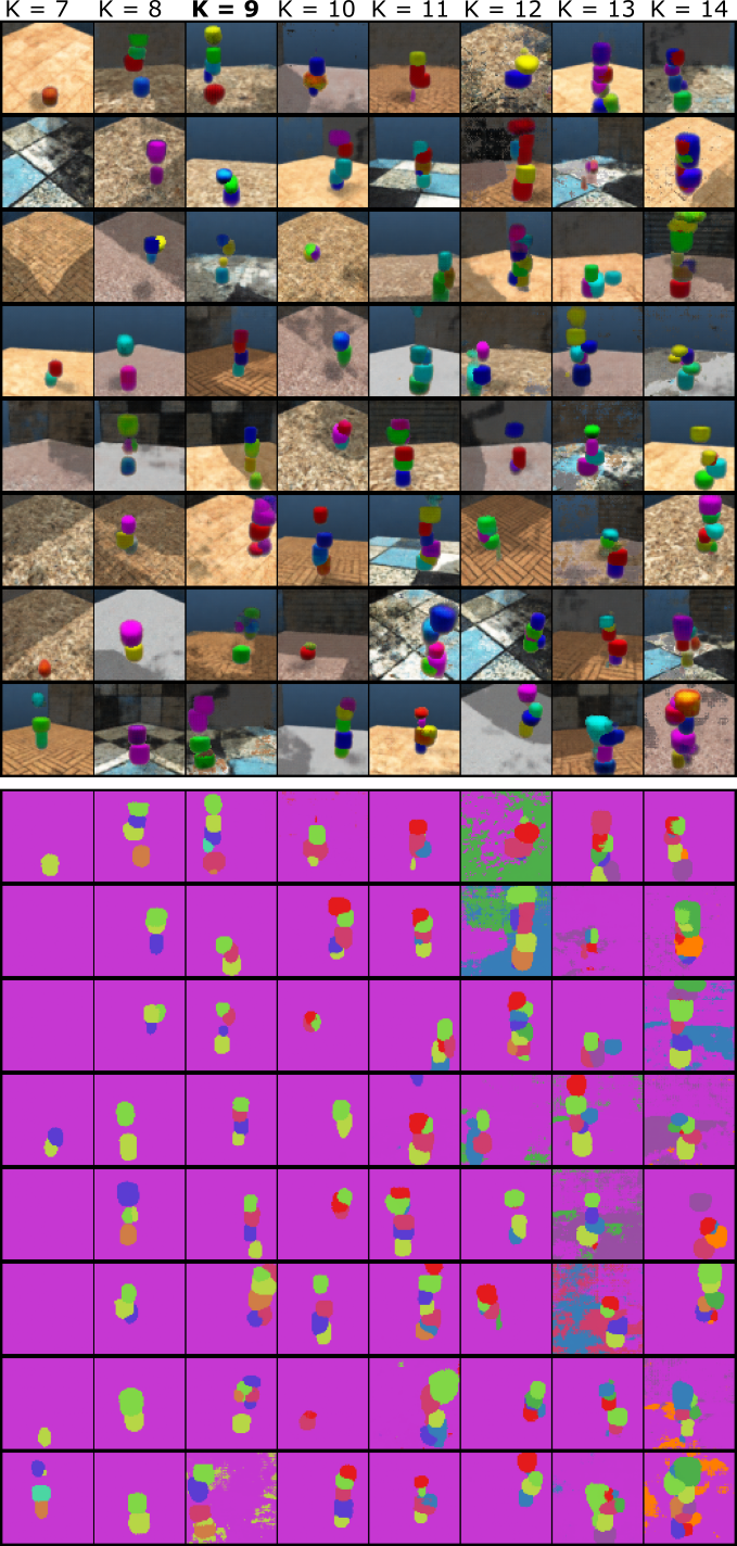
Generalizing to different numbers of slots: We demonstrate that the number of slots can be changed at test time to generate scenes with fewer or more objects than seen during training in Figure 12.

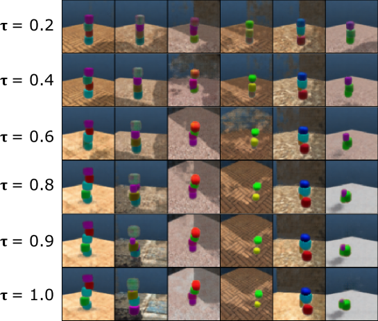
Effect of temperature scaling: We investigate whether temperature scaling provides any further qualitative improvement in sample quality (Figure 13).

Random samples from SRI-EMORL: Random samples from SRI-EMORL on CLEVR6 (visualized with temperature scaling) (Figure 14).

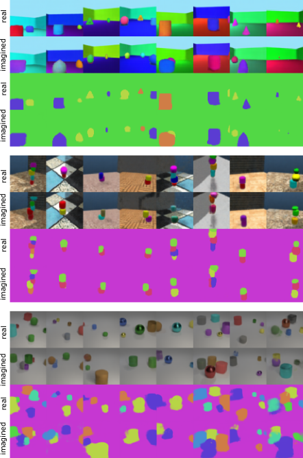
Imagination rollouts: We provide more examples of pairs of reconstructed scenes with the corresponding imagination rollout used by SRI for slot order estimation (Figure 15).

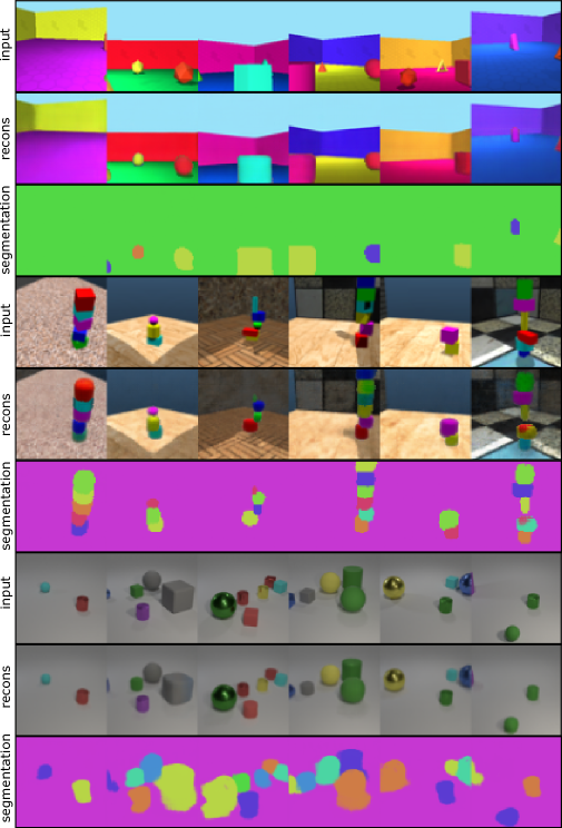
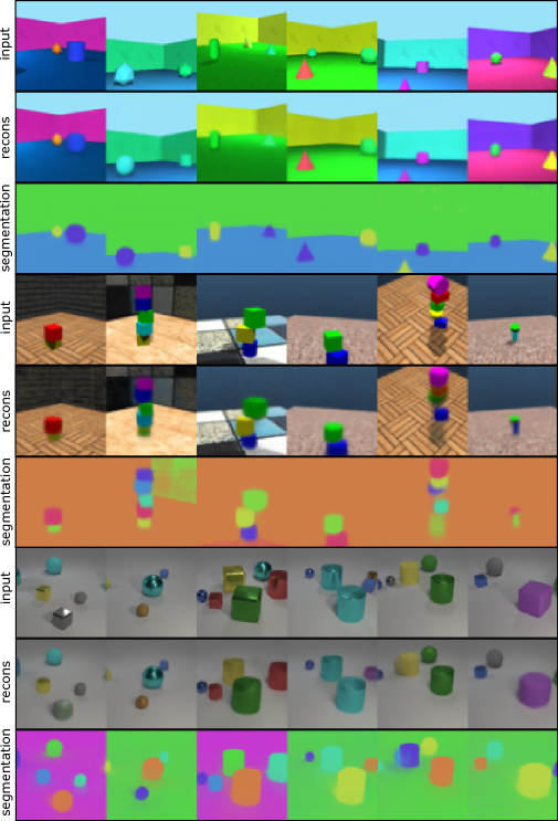
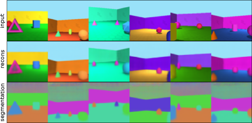
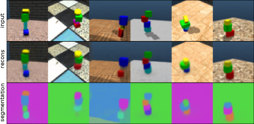
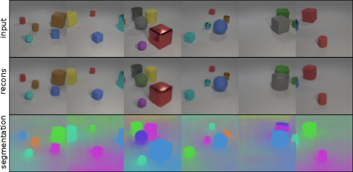
Reconstruction and segmentation examples: Examples of reconstructed and segmented scenes from each dataset for SRI-MoG (Figure 16), SRI-G (Figure 17), and GENv2-G (Figure 18).

(a) ShapeStacks images

(b) ShapeStacks masks

(c) CLEVR6 images

(d) CLEVR6 masks

(e) Objects Room images

(f) Objects Room masks

Figure 9: Additional random samples generated by SRI-MoG.

(a) ShapeStacks images

(b) ShapeStacks masks

(c) CLEVR6 images

(d) CLEVR6 masks

(e) Objects Room images

(f) Objects Room masks

Figure 10: Additional random samples generated by SRI-G.

(a) ShapeStacks images

(b) ShapeStacks masks

(c) CLEVR6 images

(d) CLEVR6 masks

(e) Objects Room images

(f) Objects Room masks

Figure 11: Additional random samples generated by GENESISv2-G.

Figure 12: Generalization to different numbers of slots $K$. Random ShapeStacks samples. SRI-MoG was trained with $K=9$.

Figure 13: Randomly sampled ShapeStacks images from SRI-MoG with different temperature scaling parameters $\tau$ in the scene-level and slot prior. Scaling down the variances in a hierarchical Gaussian prior is known to help samples stay in regions of high probability (Vahdat and Kautz, 2020). We confirm here that values of $\tau$ near 1.0 slightly improve sample quality on challenging datasets with minimal impact on sample diversity. Note that we use $\tau=1.0$ in this work for all evaluations unless stated otherwise.

(a) CLEVR6 images

(b) CLEVR6 masks

Figure 14: Random samples generated by SRI-EMORL. These images are generated with temperature $\tau=0.8$.

Figure 15: Imagination examples. Side-by-side comparisons of reconstructed RGB images and masks from SRI-MoG’s aligned autoregressive posterior with imagined RGB images and masks.

Figure 16: SRI-MoG reconstruction and segmentation.

Figure 17: SRI-G reconstruction and segmentation.

Figure 18: GENv2-G reconstruction and segmentation.

References

- Adams and Zemel (2011) Ryan Prescott Adams and Richard S Zemel. Ranking via sinkhorn propagation. ArXiv preprint, abs/1106.1925, 2011.
- Anciukevicius et al. (2020) Titas Anciukevicius, Christoph H Lampert, and Paul Henderson. Object-centric image generation with factored depths, locations, and appearances. ArXiv preprint, abs/2004.00642, 2020.
- Baillargeon (2004) Renée Baillargeon. Infants’ physical world. Current directions in psychological science, 13(3):89–94, 2004.
- Battaglia et al. (2013) Peter W Battaglia, Jessica B Hamrick, and Joshua B Tenenbaum. Simulation as an engine of physical scene understanding. Proceedings of the National Academy of Sciences, 110(45):18327–18332, 2013.
- Burgess et al. (2019) Christopher P Burgess, Loic Matthey, Nicholas Watters, Rishabh Kabra, Irina Higgins, Matt Botvinick, and Alexander Lerchner. MONet: Unsupervised scene decomposition and representation. ArXiv preprint, abs/1901.11390, 2019.
- Chen et al. (2020) Mark Chen, Alec Radford, Rewon Child, Jeffrey Wu, Heewoo Jun, David Luan, and Ilya Sutskever. Generative pretraining from pixels. In Proceedings of the 37th International Conference on Machine Learning, ICML 2020, 13-18 July 2020, Virtual Event, volume 119 of Proceedings of Machine Learning Research, pages 1691–1703. PMLR, 2020.
- Child et al. (2019) Rewon Child, Scott Gray, Alec Radford, and Ilya Sutskever. Generating long sequences with sparse transformers. ArXiv preprint, abs/1904.10509, 2019.
- Crawford and Pineau (2019) Eric Crawford and Joelle Pineau. Spatially invariant unsupervised object detection with convolutional neural networks. In The Thirty-Third AAAI Conference on Artificial Intelligence, AAAI 2019, The Thirty-First Innovative Applications of Artificial Intelligence Conference, IAAI 2019, The Ninth AAAI Symposium on Educational Advances in Artificial Intelligence, EAAI 2019, Honolulu, Hawaii, USA, January 27 - February 1, 2019, pages 3412–3420. AAAI Press, 2019. doi: 10.1609/aaai.v33i01.33013412.
- Creswell et al. (2021) Antonia Creswell, Rishabh Kabra, Chris Burgess, and Murray Shanahan. Unsupervised object-based transition models for 3d partially observable environments. Advances in Neural Information Processing Systems, 34, 2021.
- Deng et al. (2021) Fei Deng, Zhuo Zhi, Donghun Lee, and Sungjin Ahn. Generative scene graph networks. In 9th International Conference on Learning Representations, ICLR 2021, Virtual Event, Austria, May 3-7, 2021. OpenReview.net, 2021.
- Emami et al. (2021) Patrick Emami, Pan He, Sanjay Ranka, and Anand Rangarajan. Efficient iterative amortized inference for learning symmetric and disentangled multi-object representations. In Marina Meila and Tong Zhang, editors, Proceedings of the 38th International Conference on Machine Learning, ICML 2021, 18-24 July 2021, Virtual Event, volume 139 of Proceedings of Machine Learning Research, pages 2970–2981. PMLR, 2021.
- Engelcke et al. (2020) Martin Engelcke, Adam R. Kosiorek, Oiwi Parker Jones, and Ingmar Posner. GENESIS: generative scene inference and sampling with object-centric latent representations. In 8th International Conference on Learning Representations, ICLR 2020, Addis Ababa, Ethiopia, April 26-30, 2020. OpenReview.net, 2020.
- Engelcke et al. (2021) Martin Engelcke, Oiwi Parker Jones, and Ingmar Posner. GENESIS-V2: Inferring unordered object representations without iterative refinement. In M. Ranzato, A. Beygelzimer, Y. Dauphin, P.S. Liang, and J. Wortman Vaughan, editors, Advances in Neural Information Processing Systems, volume 34, pages 8085–8094. Curran Associates, Inc., 2021.
- Eslami et al. (2016) S. M. Ali Eslami, Nicolas Heess, Theophane Weber, Yuval Tassa, David Szepesvari, Koray Kavukcuoglu, and Geoffrey E. Hinton. Attend, infer, repeat: Fast scene understanding with generative models. In Daniel D. Lee, Masashi Sugiyama, Ulrike von Luxburg, Isabelle Guyon, and Roman Garnett, editors, Advances in Neural Information Processing Systems 29: Annual Conference on Neural Information Processing Systems 2016, December 5-10, 2016, Barcelona, Spain, pages 3225–3233, 2016.
- Germain et al. (2015) Mathieu Germain, Karol Gregor, Iain Murray, and Hugo Larochelle. MADE: masked autoencoder for distribution estimation. In Francis R. Bach and David M. Blei, editors, Proceedings of the 32nd International Conference on Machine Learning, ICML 2015, Lille, France, 6-11 July 2015, volume 37 of JMLR Workshop and Conference Proceedings, pages 881–889. JMLR.org, 2015.
- Glorot and Bengio (2010) Xavier Glorot and Yoshua Bengio. Understanding the difficulty of training deep feedforward neural networks. In Proceedings of the thirteenth international conference on artificial intelligence and statistics, pages 249–256. JMLR Workshop and Conference Proceedings, 2010.
- Gopalakrishnan et al. (2023) Anand Gopalakrishnan, Kazuki Irie, Jürgen Schmidhuber, and Sjoerd van Steenkiste. Unsupervised learning of temporal abstractions with slot-based transformers. Neural Computation, 35(4):593–626, 2023.
- Greff et al. (2017) Klaus Greff, Aaron Klein, Martin Chovanec, Frank Hutter, and Jürgen Schmidhuber. The sacred infrastructure for computational research. In Proceedings of the 15th python in science conference (SciPy 2017), volume 28, pages 49–56, 2017.
- Greff et al. (2019) Klaus Greff, Raphaël Lopez Kaufman, Rishabh Kabra, Nick Watters, Christopher Burgess, Daniel Zoran, Loic Matthey, Matthew Botvinick, and Alexander Lerchner. Multi-object representation learning with iterative variational inference. In Kamalika Chaudhuri and Ruslan Salakhutdinov, editors, Proceedings of the 36th International Conference on Machine Learning, ICML 2019, 9-15 June 2019, Long Beach, California, USA, volume 97 of Proceedings of Machine Learning Research, pages 2424–2433. PMLR, 2019.
- Greff et al. (2020) Klaus Greff, Sjoerd van Steenkiste, and Jürgen Schmidhuber. On the binding problem in artificial neural networks. ArXiv preprint, abs/2012.05208, 2020.
- Groth et al. (2018) Oliver Groth, Fabian B Fuchs, Ingmar Posner, and Andrea Vedaldi. Shapestacks: Learning vision-based physical intuition for generalised object stacking. In Proceedings of the European Conference on Computer Vision (ECCV), pages 702–717, 2018.
- Grover et al. (2019) Aditya Grover, Eric Wang, Aaron Zweig, and Stefano Ermon. Stochastic optimization of sorting networks via continuous relaxations. In 7th International Conference on Learning Representations, ICLR 2019, New Orleans, LA, USA, May 6-9, 2019. OpenReview.net, 2019.
- Harris et al. (2020) Charles R. Harris, K. Jarrod Millman, Stéfan J. van der Walt, Ralf Gommers, Pauli Virtanen, David Cournapeau, Eric Wieser, Julian Taylor, Sebastian Berg, Nathaniel J. Smith, Robert Kern, Matti Picus, Stephan Hoyer, Marten H. van Kerkwijk, Matthew Brett, Allan Haldane, Jaime Fernández del Río, Mark Wiebe, Pearu Peterson, Pierre Gérard-Marchant, Kevin Sheppard, Tyler Reddy, Warren Weckesser, Hameer Abbasi, Christoph Gohlke, and Travis E. Oliphant. Array programming with NumPy. Nature, 585(7825):357–362, 2020. ISSN 1476-4687. doi: 10.1038/s41586-020-2649-2.
- Hendrycks and Gimpel (2016) Dan Hendrycks and Kevin Gimpel. Gaussian error linear units (gelus). ArXiv preprint, abs/1606.08415, 2016.
- Heusel et al. (2017) Martin Heusel, Hubert Ramsauer, Thomas Unterthiner, Bernhard Nessler, and Sepp Hochreiter. GANs trained by a two time-scale update rule converge to a local nash equilibrium. In Isabelle Guyon, Ulrike von Luxburg, Samy Bengio, Hanna M. Wallach, Rob Fergus, S. V. N. Vishwanathan, and Roman Garnett, editors, Advances in Neural Information Processing Systems 30: Annual Conference on Neural Information Processing Systems 2017, December 4-9, 2017, Long Beach, CA, USA, pages 6626–6637, 2017.
- Hochreiter and Schmidhuber (1997) Sepp Hochreiter and Jürgen Schmidhuber. Long short-term memory. Neural computation, 9(8):1735–1780, 1997.
- Hubert and Arabie (1985) Lawrence Hubert and Phipps Arabie. Comparing partitions. Journal of classification, 2(1):193–218, 1985.
- Hunter (2007) J. D. Hunter. Matplotlib: A 2D Graphics Environment. Computing in Science & Engineering, 9(3):90–95, 2007.
- Jiang and Ahn (2020) Jindong Jiang and Sungjin Ahn. Generative neurosymbolic machines. In Hugo Larochelle, Marc’Aurelio Ranzato, Raia Hadsell, Maria-Florina Balcan, and Hsuan-Tien Lin, editors, Advances in Neural Information Processing Systems 33: Annual Conference on Neural Information Processing Systems 2020, NeurIPS 2020, December 6-12, 2020, virtual, 2020.
- Jurewicz and Derczynski (2021) Mateusz Jurewicz and Leon Derczynski. Set-to-sequence methods in machine learning: a review. Journal of Artificial Intelligence Research, 71:885–924, 2021.
- Kabra et al. (2019) Rishabh Kabra, Chris Burgess, Loic Matthey, Raphael Lopez Kaufman, Klaus Greff, Malcolm Reynolds, and Alexander Lerchner. Multi-object datasets, 2019.
- Kabra et al. (2021) Rishabh Kabra, Daniel Zoran, Goker Erdogan, Loic Matthey, Antonia Creswell, Matt Botvinick, Alexander Lerchner, and Chris Burgess. SIMONe: View-invariant, temporally-abstracted object representations via unsupervised video decomposition. In M. Ranzato, A. Beygelzimer, Y. Dauphin, P.S. Liang, and J. Wortman Vaughan, editors, Advances in Neural Information Processing Systems, volume 34, pages 20146–20159. Curran Associates, Inc., 2021.
- Kahneman et al. (1992) Daniel Kahneman, Anne Treisman, and Brian J Gibbs. The reviewing of object files: Object-specific integration of information. Cognitive psychology, 24(2):175–219, 1992.
- Kingma and Ba (2015) Diederik P. Kingma and Jimmy Ba. Adam: A method for stochastic optimization. In Yoshua Bengio and Yann LeCun, editors, 3rd International Conference on Learning Representations, ICLR 2015, San Diego, CA, USA, May 7-9, 2015, Conference Track Proceedings, 2015.
- Kingma and Welling (2014) Diederik P. Kingma and Max Welling. Auto-encoding variational bayes. In Yoshua Bengio and Yann LeCun, editors, 2nd International Conference on Learning Representations, ICLR 2014, Banff, AB, Canada, April 14-16, 2014, Conference Track Proceedings, 2014.
- Kluyver et al. (2016) Thomas Kluyver, Benjamin Ragan-Kelley, Fernando Pérez, Brian Granger, Matthias Bussonnier, Jonathan Frederic, Kyle Kelley, Jessica Hamrick, Jason Grout, Sylvain Corlay, Paul Ivanov, Damián Avila, Safia Abdalla, and Carol Willing. Jupyter Notebooks – a publishing format for reproducible computational workflows. In F. Loizides and B. Schmidt, editors, Positioning and Power in Academic Publishing: Players, Agents and Agendas, pages 87 – 90. IOS Press, 2016.
- Lake et al. (2017) Brenden M Lake, Tomer D Ullman, Joshua B Tenenbaum, and Samuel J Gershman. Building machines that learn and think like people. Behavioral and brain sciences, 40, 2017.
- Li et al. (2020) Nanbo Li, Cian Eastwood, and Robert B. Fisher. Learning object-centric representations of multi-object scenes from multiple views. In Hugo Larochelle, Marc’Aurelio Ranzato, Raia Hadsell, Maria-Florina Balcan, and Hsuan-Tien Lin, editors, Advances in Neural Information Processing Systems 33: Annual Conference on Neural Information Processing Systems 2020, NeurIPS 2020, December 6-12, 2020, virtual, 2020.
- Li et al. (2021a) Nanbo Li, Muhammad Ahmed Raza, Wenbin Hu, Zhaole Sun, and Robert Fisher. Object-centric representation learning with generative spatial-temporal factorization. Advances in Neural Information Processing Systems, 34, 2021a.
- Li et al. (2021b) Xuanlin Li, Brandon Trabucco, Dong Huk Park, Michael Luo, Sheng Shen, Trevor Darrell, and Yang Gao. Discovering non-monotonic autoregressive orderings with variational inference. In 9th International Conference on Learning Representations, ICLR 2021, Virtual Event, Austria, May 3-7, 2021. OpenReview.net, 2021b.
- Lin et al. (2020a) Zhixuan Lin, Yi-Fu Wu, Skand Vishwanath Peri, Bofeng Fu, Jindong Jiang, and Sungjin Ahn. Improving generative imagination in object-centric world models. In Proceedings of the 37th International Conference on Machine Learning, ICML 2020, 13-18 July 2020, Virtual Event, volume 119 of Proceedings of Machine Learning Research, pages 6140–6149. PMLR, 2020a.
- Lin et al. (2020b) Zhixuan Lin, Yi-Fu Wu, Skand Vishwanath Peri, Weihao Sun, Gautam Singh, Fei Deng, Jindong Jiang, and Sungjin Ahn. SPACE: unsupervised object-oriented scene representation via spatial attention and decomposition. In 8th International Conference on Learning Representations, ICLR 2020, Addis Ababa, Ethiopia, April 26-30, 2020. OpenReview.net, 2020b.
- Locatello et al. (2020) Francesco Locatello, Dirk Weissenborn, Thomas Unterthiner, Aravindh Mahendran, Georg Heigold, Jakob Uszkoreit, Alexey Dosovitskiy, and Thomas Kipf. Object-centric learning with slot attention. In Hugo Larochelle, Marc’Aurelio Ranzato, Raia Hadsell, Maria-Florina Balcan, and Hsuan-Tien Lin, editors, Advances in Neural Information Processing Systems 33: Annual Conference on Neural Information Processing Systems 2020, NeurIPS 2020, December 6-12, 2020, virtual, 2020.
- Mena et al. (2018) Gonzalo E. Mena, David Belanger, Scott W. Linderman, and Jasper Snoek. Learning latent permutations with gumbel-sinkhorn networks. In 6th International Conference on Learning Representations, ICLR 2018, Vancouver, BC, Canada, April 30 - May 3, 2018, Conference Track Proceedings. OpenReview.net, 2018.
- Mishkin et al. (2022) Pamela Mishkin, Lama Ahmad, Miles Brundage, Gretchen Krueger, and Girish Sastry. Dall·e 2 preview - risks and limitations. 2022.
- Munkres (1957) James Munkres. Algorithms for the assignment and transportation problems. Journal of the society for industrial and applied mathematics, 5(1):32–38, 1957.
- Parmar et al. (2018) Niki Parmar, Ashish Vaswani, Jakob Uszkoreit, Lukasz Kaiser, Noam Shazeer, Alexander Ku, and Dustin Tran. Image transformer. In Jennifer G. Dy and Andreas Krause, editors, Proceedings of the 35th International Conference on Machine Learning, ICML 2018, Stockholmsmässan, Stockholm, Sweden, July 10-15, 2018, volume 80 of Proceedings of Machine Learning Research, pages 4052–4061. PMLR, 2018.
- Paszke et al. (2019) Adam Paszke, Sam Gross, Francisco Massa, Adam Lerer, James Bradbury, Gregory Chanan, Trevor Killeen, Zeming Lin, Natalia Gimelshein, Luca Antiga, Alban Desmaison, Andreas Kopf, Edward Yang, Zachary DeVito, Martin Raison, Alykhan Tejani, Sasank Chilamkurthy, Benoit Steiner, Lu Fang, Junjie Bai, and Soumith Chintala. PyTorch: An Imperative Style, High-Performance Deep Learning Library. In Advances in Neural Information Processing Systems 32, pages 8024–8035. Curran Associates, Inc., 2019.
- Pedregosa et al. (2011) Fabian Pedregosa, Gaël Varoquaux, Alexandre Gramfort, Vincent Michel, Bertrand Thirion, Olivier Grisel, Mathieu Blondel, Peter Prettenhofer, Ron Weiss, Vincent Dubourg, Jake Vanderplas, Alexandre Passos, David Cournapeau, Matthieu Brucher, Matthieu Perrot, and Édouard Duchesnay. Scikit-learn: Machine Learning in Python. Journal of Machine Learning Research, 12(85):2825–2830, 2011.
- Rand (1971) William M Rand. Objective criteria for the evaluation of clustering methods. Journal of the American Statistical association, 66(336):846–850, 1971.
- Rezende and Viola (2018) Danilo Jimenez Rezende and Fabio Viola. Taming VAEs. ArXiv preprint, abs/1810.00597, 2018.
- Rezende et al. (2014) Danilo Jimenez Rezende, Shakir Mohamed, and Daan Wierstra. Stochastic backpropagation and approximate inference in deep generative models. In Proceedings of the 31th International Conference on Machine Learning, ICML 2014, Beijing, China, 21-26 June 2014, volume 32 of JMLR Workshop and Conference Proceedings, pages 1278–1286. JMLR.org, 2014.
- Salimans et al. (2017) Tim Salimans, Andrej Karpathy, Xi Chen, and Diederik P. Kingma. Pixelcnn++: Improving the pixelcnn with discretized logistic mixture likelihood and other modifications. In 5th International Conference on Learning Representations, ICLR 2017, Toulon, France, April 24-26, 2017, Conference Track Proceedings. OpenReview.net, 2017.
- Santoro et al. (2017) Adam Santoro, David Raposo, David G. T. Barrett, Mateusz Malinowski, Razvan Pascanu, Peter W. Battaglia, and Tim Lillicrap. A simple neural network module for relational reasoning. In Isabelle Guyon, Ulrike von Luxburg, Samy Bengio, Hanna M. Wallach, Rob Fergus, S. V. N. Vishwanathan, and Roman Garnett, editors, Advances in Neural Information Processing Systems 30: Annual Conference on Neural Information Processing Systems 2017, December 4-9, 2017, Long Beach, CA, USA, pages 4967–4976, 2017.
- Schölkopf et al. (2021) Bernhard Schölkopf, Francesco Locatello, Stefan Bauer, Nan Rosemary Ke, Nal Kalchbrenner, Anirudh Goyal, and Yoshua Bengio. Toward causal representation learning. Proceedings of the IEEE, 109(5):612–634, 2021.
- Seitzer et al. (2023) Maximilian Seitzer, Max Horn, Andrii Zadaianchuk, Dominik Zietlow, Tianjun Xiao, Carl-Johann Simon-Gabriel, Tong He, Zheng Zhang, Bernhard Schölkopf, Thomas Brox, et al. Bridging the gap to real-world object-centric learning. In 11th International Conference on Learning Representations, ICLR 2023, 2023.
- Singh et al. (2022) Gautam Singh, Fei Deng, and Sungjin Ahn. Illiterate DALL-E learns to compose. In 10th International Conference on Learning Representations, ICLR 2022, 2022.
- Spelke and Kinzler (2007) Elizabeth S Spelke and Katherine D Kinzler. Core knowledge. Developmental science, 10(1):89–96, 2007.
- Stelzner et al. (2021) Karl Stelzner, Kristian Kersting, and Adam R Kosiorek. Decomposing 3d scenes into objects via unsupervised volume segmentation. ArXiv preprint, abs/2104.01148, 2021.
- Uria et al. (2016) Benigno Uria, Marc-Alexandre Côté, Karol Gregor, Iain Murray, and Hugo Larochelle. Neural autoregressive distribution estimation. The Journal of Machine Learning Research, 17(1):7184–7220, 2016.
- Vahdat and Kautz (2020) Arash Vahdat and Jan Kautz. NVAE: A deep hierarchical variational autoencoder. In Hugo Larochelle, Marc’Aurelio Ranzato, Raia Hadsell, Maria-Florina Balcan, and Hsuan-Tien Lin, editors, Advances in Neural Information Processing Systems 33: Annual Conference on Neural Information Processing Systems 2020, NeurIPS 2020, December 6-12, 2020, virtual, 2020.
- van den Oord et al. (2016) Aäron van den Oord, Nal Kalchbrenner, Lasse Espeholt, Koray Kavukcuoglu, Oriol Vinyals, and Alex Graves. Conditional image generation with pixelcnn decoders. In Daniel D. Lee, Masashi Sugiyama, Ulrike von Luxburg, Isabelle Guyon, and Roman Garnett, editors, Advances in Neural Information Processing Systems 29: Annual Conference on Neural Information Processing Systems 2016, December 5-10, 2016, Barcelona, Spain, pages 4790–4798, 2016.
- Van Oord et al. (2016) Aaron Van Oord, Nal Kalchbrenner, and Koray Kavukcuoglu. Pixel recurrent neural networks. In International conference on machine learning, pages 1747–1756. PMLR, 2016.
- Vaswani et al. (2017) Ashish Vaswani, Noam Shazeer, Niki Parmar, Jakob Uszkoreit, Llion Jones, Aidan N. Gomez, Lukasz Kaiser, and Illia Polosukhin. Attention is all you need. In Isabelle Guyon, Ulrike von Luxburg, Samy Bengio, Hanna M. Wallach, Rob Fergus, S. V. N. Vishwanathan, and Roman Garnett, editors, Advances in Neural Information Processing Systems 30: Annual Conference on Neural Information Processing Systems 2017, December 4-9, 2017, Long Beach, CA, USA, pages 5998–6008, 2017.
- Veerapaneni et al. (2019) Rishi Veerapaneni, John D Co-Reyes, Michael Chang, Michael Janner, Chelsea Finn, Jiajun Wu, Joshua B Tenenbaum, and Sergey Levine. Entity abstraction in visual model-based reinforcement learning. ArXiv preprint, abs/1910.12827, 2019.
- Vinyals et al. (2015) Oriol Vinyals, Meire Fortunato, and Navdeep Jaitly. Pointer networks. In Corinna Cortes, Neil D. Lawrence, Daniel D. Lee, Masashi Sugiyama, and Roman Garnett, editors, Advances in Neural Information Processing Systems 28: Annual Conference on Neural Information Processing Systems 2015, December 7-12, 2015, Montreal, Quebec, Canada, pages 2692–2700, 2015.
- Vinyals et al. (2016) Oriol Vinyals, Samy Bengio, and Manjunath Kudlur. Order matters: Sequence to sequence for sets. In Yoshua Bengio and Yann LeCun, editors, 4th International Conference on Learning Representations, ICLR 2016, San Juan, Puerto Rico, May 2-4, 2016, Conference Track Proceedings, 2016.
- von Kügelgen et al. (2020) Julius von Kügelgen, Ivan Ustyuzhaninov, Peter Gehler, Matthias Bethge, and Bernhard Schölkopf. Towards causal generative scene models via competition of experts. ArXiv preprint, abs/2004.12906, 2020.
- Watters et al. (2019a) Nicholas Watters, Loic Matthey, Matko Bosnjak, Christopher P Burgess, and Alexander Lerchner. COBRA: data-efficient model-based rl through unsupervised object discovery and curiosity-driven exploration. ArXiv preprint, abs/1905.09275, 2019a.
- Watters et al. (2019b) Nicholas Watters, Loic Matthey, Christopher P Burgess, and Alexander Lerchner. Spatial broadcast decoder: A simple architecture for learning disentangled representations in vaes. ArXiv preprint, abs/1901.07017, 2019b.
- Yang et al. (2019) Zhilin Yang, Zihang Dai, Yiming Yang, Jaime G. Carbonell, Ruslan Salakhutdinov, and Quoc V. Le. XLNet: generalized autoregressive pretraining for language understanding. In Hanna M. Wallach, Hugo Larochelle, Alina Beygelzimer, Florence d’Alché-Buc, Emily B. Fox, and Roman Garnett, editors, Advances in Neural Information Processing Systems 32: Annual Conference on Neural Information Processing Systems 2019, NeurIPS 2019, December 8-14, 2019, Vancouver, BC, Canada, pages 5754–5764, 2019.
- Yu et al. (2021) Hong-Xing Yu, Leonidas J Guibas, and Jiajun Wu. Unsupervised discovery of object radiance fields. ArXiv preprint, abs/2107.07905, 2021.
- Yuan et al. (2021) Jinyang Yuan, Bin Li, and Xiangyang Xue. Unsupervised learning of compositional scene representations from multiple unspecified viewpoints. ArXiv preprint, abs/2112.03568, 2021.
- Yuille and Kersten (2006) Alan Yuille and Daniel Kersten. Vision as bayesian inference: analysis by synthesis? Trends in cognitive sciences, 10(7):301–308, 2006.
- Zablotskaia et al. (2021) Polina Zablotskaia, Edoardo A Dominici, Leonid Sigal, and Andreas M Lehrmann. PROVIDE: a probabilistic framework for unsupervised video decomposition. In Uncertainty in Artificial Intelligence, pages 2019–2028. PMLR, 2021.
- Zaheer et al. (2017) Manzil Zaheer, Satwik Kottur, Siamak Ravanbakhsh, Barnabás Póczos, Ruslan Salakhutdinov, and Alexander J. Smola. Deep sets. In Isabelle Guyon, Ulrike von Luxburg, Samy Bengio, Hanna M. Wallach, Rob Fergus, S. V. N. Vishwanathan, and Roman Garnett, editors, Advances in Neural Information Processing Systems 30: Annual Conference on Neural Information Processing Systems 2017, December 4-9, 2017, Long Beach, CA, USA, pages 3391–3401, 2017.
- Zhang et al. (2019) Yan Zhang, Jonathon S. Hare, and Adam Prügel-Bennett. Learning representations of sets through optimized permutations. In 7th International Conference on Learning Representations, ICLR 2019, New Orleans, LA, USA, May 6-9, 2019. OpenReview.net, 2019.
- Zhu et al. (2020) Yixin Zhu, Tao Gao, Lifeng Fan, Siyuan Huang, Mark Edmonds, Hangxin Liu, Feng Gao, Chi Zhang, Siyuan Qi, Ying Nian Wu, et al. Dark, beyond deep: A paradigm shift to cognitive ai with humanlike common sense. Engineering, 6(3):310–345, 2020.
- Zoran et al. (2021) Daniel Zoran, Rishabh Kabra, Alexander Lerchner, and Danilo J Rezende. PARTS: unsupervised segmentation with slots, attention and independence maximization. In Proceedings of the IEEE/CVF International Conference on Computer Vision, pages 10439–10447, 2021.