Adversarial Unlearning:
Reducing Confidence Along Adversarial Directions

Amrith Setlur1,   Benjamin Eysenbach1   Virginia Smith1   Sergey Levine2
1 Carnegie Mellon University  2 UC Berkeley
Correspondence can be sent to asetlur@cs.cmu.edu.
Abstract

Supervised learning methods trained with maximum likelihood objectives often overfit on training data. Most regularizers that prevent overfitting look to increase confidence on additional examples (e.g., data augmentation, adversarial training), or reduce it on training data (e.g., label smoothing). In this work we propose a complementary regularization strategy that reduces confidence on self-generated examples. The method, which we call RCAD (Reducing Confidence along Adversarial Directions), aims to reduce confidence on out-of-distribution examples lying along directions adversarially chosen to increase training loss. In contrast to adversarial training, RCAD does not try to robustify the model to output the original label, but rather regularizes it to have reduced confidence on points generated using much larger perturbations than in conventional adversarial training. RCAD can be easily integrated into training pipelines with a few lines of code. Despite its simplicity, we find on many classification benchmarks that RCAD can be added to existing techniques (e.g., label smoothing, MixUp training) to increase test accuracy by 1–3%percent\% in absolute value, with more significant gains in the low data regime. We also provide a theoretical analysis that helps to explain these benefits in simplified settings, showing that RCAD can provably help the model unlearn spurious features in the training data.

1 Introduction

Supervised learning techniques typically consider training models to make accurate predictions on fresh test examples drawn from the same distribution as training data. Unfortunately, it is well known that maximizing the likelihood of the training data alone may result in overfitting. Prior work broadly considers two approaches to combat this issue. Some methods train on additional examples, e.g., generated via augmentations [52, 9, 65] or adversarial updates [13, 35, 3]. Others modify the objective by using alternative losses and/or regularization terms (e.g., label smoothing [55, 38], MixUp [68], robust objectives [64, 21]). In effect, these prior approaches either make the model’s predictions more certain on new training examples or make the distribution over potential models less certain.

Existing regularization methods can be seen as providing a certain inductive bias for the model, e.g., the model’s weights should be small (i.e., weight decay), the model’s predictions should vary linearly between training examples (i.e., MixUp). In this paper we identify a different inductive bias: the model’s predictions should be less confident on out-of-distribution inputs that look nothing like the training examples. We turn this form of inductive bias into a simple regularizer, whose benefits are complementary to existing regularization strategies. To instantiate such a method, we must be able to sample out-of-distribution examples. For this, we propose a simple approach: generating adversarial examples [37, 13] using very large step sizes (orders-of-magnitude larger than traditional adversarial training [35]). Hence, we first perturb the training points using the training loss gradient, and then maximize predictive entropy on these adversarially perturbed examples.

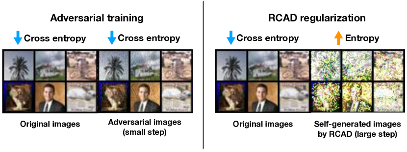
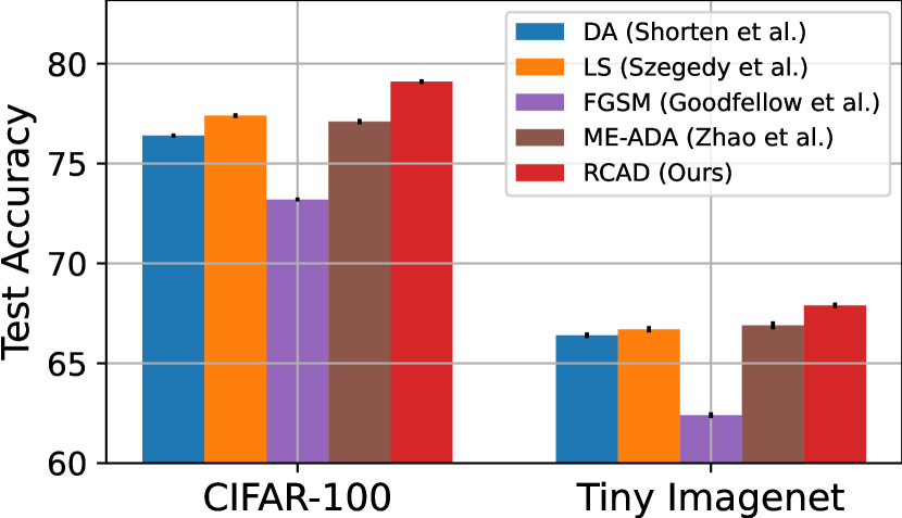
In contrast to adversarial training, our method does not try to robustify the model to output the original label, but rather regularizes it to have reduced confidence on examples generated via a large step size (Figure 1(a)). As shown in Figure 1(b), this can lead to significant improvements in in-distribution test accuracy unlike adversarial training [35, 36, 4, 3], which tends to decrease in-distribution test performance [47, 69, 60]. Compared with semi-supervised learning methods [14, 63], our method does not require an additional unlabeled dataset (it generates one automatically), and different from prior works [63, 73] it also trains the model to be less confident on these examples.

As the self-generated samples in our procedure no longer resemble in-distribution data, we are uncertain of their labels and train the model to predict a uniform distribution over labels on them, following the principle of maximum entropy [24]. A few prior works [55, 42, 51, 10] have also considered using the same principle to prevent the memorization of training examples, but only increase entropy on iid sampled in-distribution labeled/unlabeled data. In contrast, we study the effect of maximizing entropy on self-generated out-of-distribution examples along adversarial directions.
Refer to caption
(a)
Refer to caption
(b)
Figure 1: Reducing confidence along adversarial directions (RCAD) is a simple and efficient regularization technique to improve test performance. (Left) For RCAD, examples are generated by taking a large step (10×10\times typical for adversarial examples) along the gradient direction. We see that generated images thus look very different from the original, with accentuated spurious components responsible for the model’s flipped predictions on adversarial images. (Right) RCAD achieves greater test accuracy than data augmentation (DA), label smoothing (LS), and methods that minimize cross-entropy on adversarial examples: adversarial training via FGSM [13] and ME-ADA [72].

The main contribution of this work is a training procedure we call RCAD: Reducing Confidence along Adversarial Directions. RCAD improves test accuracy (for classification) and log-likelihood (for regression) across multiple supervised learning benchmarks. Importantly, we find that the benefits of RCAD are complementary to prior methods: Combining RCAD with alternative regularizers (e.g., augmentation [52, 65], label smoothing [55], MixUp training [68]) further improves performance. Our method requires adding similar-to\sim5 lines of code and is computationally efficient (with training time at most 1.3×1.3\times standard). We provide a theoretical analysis that helps to explain RCAD’s benefits in a simplified setting, showing that RCAD can unlearn spurious features in the training data, thereby improving accuracy on unseen examples.

2 Related Work

Table 1: Regularization objectives: We summarize prior works that employ adversarial examples or directly regularize model’s predictions p𝒘(y𝐱)subscript𝑝𝒘conditionaly𝐱p_{\bm{w}}({\textnormal{y}}\mid{\mathbf{x}}) along with the scalar hyperparameters (in []delimited-[][\cdot]) associated with each.
name objective
cross entropy min𝒘𝐱,y𝒟^logp𝒘(y𝐱)subscript𝒘subscript𝐱y^𝒟subscript𝑝𝒘conditionaly𝐱\min_{{\bm{w}}}-\sum_{{{\mathbf{x}},{\textnormal{y}}}\in\hat{\mathcal{D}}}\log p_{\bm{w}}({\textnormal{y}}\mid{\mathbf{x}})
label smoothing [ϵ]delimited-[]italic-ϵ[\epsilon] [38] min𝒘𝐱,y𝒟^((1ϵ)logp𝒘(y𝐱)+yyϵ|𝒴|1logp𝒘(y𝐱))subscript𝒘subscript𝐱y^𝒟1italic-ϵsubscript𝑝𝒘conditionaly𝐱subscriptsuperscript𝑦yitalic-ϵ𝒴1subscript𝑝𝒘conditionalsuperscript𝑦𝐱\min_{\bm{w}}-\sum_{{{\mathbf{x}},{\textnormal{y}}}\in\hat{\mathcal{D}}}\left((1-\epsilon)\log p_{\bm{w}}({\textnormal{y}}\mid{\mathbf{x}})+\sum_{y^{\prime}\neq{\textnormal{y}}}\frac{\epsilon}{|{\mathcal{Y}}|-1}\log p_{\bm{w}}(y^{\prime}\mid{\mathbf{x}})\right)
Adv. training [α]delimited-[]𝛼[\alpha] [35] min𝒘𝐱,y𝒟^logp𝒘(y𝐱αsign(𝐱logp𝒘(y𝐱)))\min_{\bm{w}}-\sum_{{{\mathbf{x}},{\textnormal{y}}}\in\hat{\mathcal{D}}}\log p_{\bm{w}}({\textnormal{y}}\mid{\mathbf{x}}-\alpha\cdot\mathrm{sign}(\nabla_{\mathbf{x}}\log p_{\bm{w}}({\textnormal{y}}\mid{\mathbf{x}})))
ME-ADA [α,β]𝛼𝛽[\alpha,\beta] [72] min𝒘(𝐱,y)𝒟^𝒟^logp𝒘(y𝐱)where, for a distance metric C𝒘:(𝒳×𝒴)×(𝒳×𝒴):subscript𝒘subscript𝐱y^𝒟superscript^𝒟subscript𝑝𝒘conditionaly𝐱where, for a distance metric subscript𝐶𝒘maps-to𝒳𝒴𝒳𝒴\min_{\bm{w}}-\sum_{({\mathbf{x}},{\textnormal{y}})\in\hat{\mathcal{D}}\cup\hat{\mathcal{D}}^{\prime}}\log p_{\bm{w}}({\textnormal{y}}\mid{\mathbf{x}})\quad\textrm{where, for a distance metric }C_{\bm{w}}\mathrm{:}({\mathcal{X}}\times{\mathcal{Y}})\times({\mathcal{X}}\times{\mathcal{Y}})\mapsto\operatorname{\mathbb{R}}
𝒟^{(𝒙~,y)𝒙~sup𝒙0logpw(𝒙0y)+α𝒘(𝒙0)βC𝒘((𝒙0,y),(𝐱,y)),(𝐱,y)𝒟^}superscript^𝒟conditional-set~𝒙yformulae-sequence~𝒙subscriptsupremumsubscript𝒙0subscript𝑝𝑤conditionalsubscript𝒙0y𝛼subscript𝒘subscript𝒙0𝛽subscript𝐶𝒘subscript𝒙0y𝐱yfor-all𝐱y^𝒟\hat{\mathcal{D}}^{\prime}\triangleq\{(\tilde{{\bm{x}}},{\textnormal{y}})\mid\tilde{{\bm{x}}}\triangleq\sup_{{\bm{x}}_{0}}-\log p_{w}({\bm{x}}_{0}\mid{\textnormal{y}})+\alpha{\mathcal{H}}_{\bm{w}}({\bm{x}}_{0})-\beta C_{\bm{w}}(({\bm{x}}_{0},{\textnormal{y}}),({\mathbf{x}},{\textnormal{y}})),\,\forall({\mathbf{x}},{\textnormal{y}})\in\hat{\mathcal{D}}\}
RCAD (ours) [α,λ]𝛼𝜆[\alpha,\lambda] min𝒘𝐱,y𝒟^(logp𝒘(y𝐱)λ𝒘(𝐱α𝐱logp𝒘(y𝐱)))subscript𝒘subscript𝐱y^𝒟subscript𝑝𝒘conditionaly𝐱𝜆subscript𝒘𝐱𝛼subscript𝐱subscript𝑝𝒘conditionaly𝐱\min_{\bm{w}}\sum_{{{\mathbf{x}},{\textnormal{y}}}\in\hat{\mathcal{D}}}\left(-\log p_{\bm{w}}({\textnormal{y}}\mid{\mathbf{x}})-\lambda\cdot{\mathcal{H}}_{\bm{w}}({\mathbf{x}}-\alpha\cdot\nabla_{\mathbf{x}}\log p_{\bm{w}}({\textnormal{y}}\mid{\mathbf{x}}))\right)

Below we survey common regularization techniques in machine learning, as well as other methods that utilize entropy maximization in training for various purposes (differing from our own).

Data augmentation. A common strategy to improve test accuracy (particularly on image tasks) is to augment the training data with corruptions [52] or surface level variations [9, 65] (e.g., rotations, random crops). Some methods [36, 35, 13] further augment data with imperceptibly different adversarial examples or interpolated samples [68]. Others [45, 41] sample new examples from generative models that model the marginal density of the input distribution. Also related are semi-supervised methods, which assume access to an extra set of unlabeled data and train the model to have more confident predictions on them [14, 36]. All these methods minimize entropy [15] on the augmented or unlabeled data to improve generalization [68, 72]. In contrast, our method maximizes entropy on perturbed samples along the adversarial direction.

Adversarial training. Deep learning models are vulnerable to worst-case perturbations that can flip the model’s predictions [13, 49]. Adversarial training was proposed to improve robustness to such attacks by reducing worst-case loss in small regions around the training samples [35, 32, 47]. More recently, Zhao et al., [72] proposed maximum entropy adversarial data augmentation (ME-ADA), which uses an information bottleneck principle to identify worst-case perturbations that both maximize training loss and predictive entropy. Similar to adversarial training ME-ADA still minimizes cross-entropy to output the same label on new points. There are two key differences between above methods and RCAD; (i) rather than minimizing cross entropy loss on adversarial examples, we increase model’s uncertainty on the self-generated examples; and (ii) we take much larger steps—so large that unlike adversarial images, the generated example is no longer similar to the original one (Figure 1(a)). We show that these differences are important to improve test performance since adversarial training has been shown to hurt generalization on non-adversarial in-distribution test points [47, 59, 69]. Further, RCAD has a lower (at most 1/5th1superscript5th1/5^{\textrm{th}}) computational cost compared to multi-step adversarial training procedures [72, 69].

Robust objectives. In order to improve robustness to noise and outliers in the data, a common approach is to modify the objective by considering risk averse loss functions [e.g., 21, 48, 56] or incorporating regularization terms such as the l2/l1subscript𝑙2subscript𝑙1l_{2}/l_{1} norms [30, 58]. Our method is similar to these approaches in that we propose a new regularization term. However, whereas most regularization terms are applied to the model’s weights or activations, ours is directly applied to the model’s predictions. Another effective loss function for classification problems is label smoothing [55, 7, 25], which uniformly increases model’s predictive uncertainty in a region around training samples [11]. In contrast, RCAD increases entropy only on examples generated along the adversarial direction that has been shown to comprise of spurious features [22, 6], thereby unlearning them.

Entropy maximization. Finally, we note that our work builds upon prior work that draws connections between entropy maximization in supervised  [51, 10, 42] and reinforcement learning [16]. For example, Pereyra et al., [42] apply a hinge form of confidence penalty directly on training data which is similar to label smoothing in principle and performance (Table 2 in [42]). Other works like [10, 51] also adapt the principle of entropy maximization but do so either on additional unlabeled data or a subset of the training samples. More recently [44] show that maximizing entropy on interpolated samples from the same class improves out-of-distribution uncertainty quantification. In contrast to the above, we minimize cross-entropy loss on training data and only maximize entropy on samples generated along the adversarial direction. Our experimental results also span a wider set of benchmarks and presents significant gains +11+13%percent33\% complementary to methods like label smoothing. We also theoretically analyze our objective for the class of linear predictors and show how RCAD can mitigate vulnerability to spurious correlations.

3 RCAD: Reducing Confidence Along Adversarial Directions

We now introduce our regularization technique for reducing confidence along adversarial directions (RCAD). This section describes the objective and an algorithm for optimizing it; Section 5 presents a more formal discussion of RCAD and in Section 4 we provide our empirical study.

Notation. We are given a training dataset 𝒟^{(𝐱(i),y(i))}i=1N^𝒟superscriptsubscriptsuperscript𝐱𝑖superscripty𝑖𝑖1𝑁\hat{\mathcal{D}}\triangleq\left\{({\mathbf{x}}^{(i)},{\textnormal{y}}^{(i)})\right\}_{i=1}^{N} where 𝐱(i)𝒳,yi𝒴formulae-sequencesuperscript𝐱𝑖𝒳superscripty𝑖𝒴{\mathbf{x}}^{(i)}\in\mathcal{X},\,{\textnormal{y}}^{i}\in{\mathcal{Y}}, are sampled iid from a joint distribution 𝒟𝒟\mathcal{D} over 𝒳×𝒴𝒳𝒴\mathcal{X}\times\mathcal{Y}. We use 𝒟^^𝒟\hat{\mathcal{D}} to denote both the training dataset and an empirical measure over it. The aim is to learn a parameterized distribution p𝒘(y𝐱),𝒘𝒲subscript𝑝𝒘conditionaly𝐱𝒘𝒲p_{\bm{w}}({\textnormal{y}}\mid{\mathbf{x}}),\;{\bm{w}}\in{\mathcal{W}} where the learnt model is typically obtained by maximizing the log-likelihood over 𝒟^^𝒟\hat{\mathcal{D}}. Such a solution is referred to as the maximum likelihood estimate (MLE): 𝒘^mleargmax𝒘𝒲𝔼𝒟^logp𝒘(y𝐱)subscript^𝒘mlesubscriptargmax𝒘𝒲subscript𝔼^𝒟subscript𝑝𝒘conditionaly𝐱\hat{{\bm{w}}}_{\mathrm{mle}}\triangleq\operatorname*{arg\,max}_{{\bm{w}}\in\mathcal{W}}\;\mathbb{E}_{\hat{\mathcal{D}}}\log p_{\bm{w}}({\textnormal{y}}\mid{\mathbf{x}}). In the classification setting, we measure the performance of any learned solution 𝒘^^𝒘\hat{{\bm{w}}} using its accuracy on the test (population) data: 𝔼𝒟[𝟙(argmaxyp𝒘^(y𝐱)=y)]subscript𝔼𝒟delimited-[]1subscriptargmaxsuperscript𝑦subscript𝑝^𝒘conditionalsuperscript𝑦𝐱y\mathbb{E}_{\mathcal{D}}\left[\mathbbm{1}(\operatorname*{arg\,max}_{y^{\prime}}p_{\hat{{\bm{w}}}}(y^{\prime}\mid{\mathbf{x}})={\textnormal{y}})\right].

Solely optimizing the log-likelihood over the training data can lead to poor test accuracy, since the estimate 𝒘^mlesubscript^𝒘mle\hat{{\bm{w}}}_{\mathrm{mle}} can overfit on noise in 𝒟^^𝒟\hat{{\mathcal{D}}} and fail to generalize to unseen samples. Many algorithms aim to mitigate overfitting by either designing suitable loss functions replacing the log-likelihood objective, or by augmenting the training set with additional data (see Section 2). Our main contribution is a new data-dependent regularization term that will depend not just on the model parameters but also on the training dataset. We reduce confidence on out-of-distribution samples that are obtained by perturbing the original inputs along the direction that adversarially maximizes training loss.

In the paragraphs that follow we describe the methodology and rationale behind our objective that uses the following definition of model’s predictive entropy when 𝒴𝒴{\mathcal{Y}} is a discrete set:

𝒘(x)y𝒴p𝒘(y𝐱)logp𝒘(y𝐱).subscript𝒘𝑥subscript𝑦𝒴subscript𝑝𝒘conditional𝑦𝐱subscript𝑝𝒘conditional𝑦𝐱\displaystyle\mathcal{H}_{\bm{w}}(x)\;\triangleq\;-\sum_{y\in{\mathcal{Y}}}p_{\bm{w}}(y\mid{\mathbf{x}})\;\log p_{\bm{w}}(y\mid{\mathbf{x}}).

In cases where 𝒴𝒴{\mathcal{Y}} is continuous, for example in regression tasks, we will use the differential form of predictive entropy: 𝒴p𝒘(y𝐱)logp𝒘(y𝐱)𝑑ysubscript𝒴subscript𝑝𝒘conditional𝑦𝐱subscript𝑝𝒘conditional𝑦𝐱differential-d𝑦-\int_{{\mathcal{Y}}}p_{\bm{w}}(y\mid{\mathbf{x}})\;\log p_{\bm{w}}(y\mid{\mathbf{x}})\;dy.

RCAD: Reducing Confidence along Adversarial Directions
def rcad_loss(x, y, |$\alpha$|, |$\lambda$|):
loss = |$-$| model(x).log_prob(y)
x_adv = x + |$\alpha$| * loss.grad(x)
entropy = model(x_adv).entropy()
return loss - |$\lambda$| * entropy

Reducing Confidence Along Adversarial Directions. The key idea behind RCAD is that models should not only make accurate predictions on the sampled data, but also make uncertain predictions on examples that are very different from training data. We use directions that adversarially maximize the training loss locally around the training points to construct these out-of-distribution examples that are different from the training data. This is mainly because adversarial directions have been known to comprise of spurious features [22] and we want to regularize the model in a way that makes it uncertain on these features. We first describe how these examples are generated, and then describe how we train the model to be less confident.

We generate an out-of-distribution example 𝐱~~𝐱\tilde{{\mathbf{x}}} by taking a large gradient of the MLE objective with respect to the input 𝐱𝐱{\mathbf{x}}, using a step size of α>0𝛼0\alpha>0:

𝐱~𝐱α𝐱logp𝒘(y𝐱)~𝐱𝐱𝛼subscript𝐱subscript𝑝𝒘conditionaly𝐱\displaystyle\tilde{{\mathbf{x}}}\;\triangleq\;{\mathbf{x}}-\alpha\cdot\nabla_{{\mathbf{x}}}\log p_{\bm{w}}({\textnormal{y}}\mid{\mathbf{x}}) (1)

We train the model to make unconfident predictions on these self-generated examples by maximizing the model’s predictive entropy. We add this entropy term 𝒘(𝐱~)subscript𝒘~𝐱\mathcal{H}_{\bm{w}}\left(\tilde{{\mathbf{x}}}\right) to the standard MLE objective, weighted by scalar λ>0𝜆0\lambda>0, yielding the final RCAD objective:

𝒘^rcadsubscript^𝒘rcad\displaystyle\hat{{\bm{w}}}_{\textrm{rcad}}\;\; argmax𝒘𝒲𝔼𝒟^[logp𝒘(y𝐱)+λ𝒘(𝐱α𝐱logp𝒘(y𝐱))]absentsubscriptargmax𝒘𝒲subscript𝔼^𝒟delimited-[]subscript𝑝𝒘conditionaly𝐱𝜆subscript𝒘𝐱𝛼subscript𝐱subscript𝑝𝒘conditionaly𝐱\displaystyle\triangleq\;\;\operatorname*{arg\,max}_{{\bm{w}}\in\mathcal{W}}\;\mathbb{E}_{\hat{\mathcal{D}}}\left[\log p_{\bm{w}}({\textnormal{y}}\mid{\mathbf{x}})+\lambda\cdot\mathcal{H}_{\bm{w}}\left({\mathbf{x}}-\alpha\cdot\nabla_{{\mathbf{x}}}\log p_{\bm{w}}({\textnormal{y}}\mid{\mathbf{x}})\right)\right] (2)

In adversarial training, adversarial examples are generated by solving a constrained optimization problem [35, 47]. Using a first-order approximation, the adversarial example 𝐱~~𝐱\tilde{{\mathbf{x}}} generated by one of the simplest solvers [13] has a closed form resembling Equation 1. We note that RCAD is different from the above form of adversarial training in two ways. First, RCAD uses a much larger step size (10×10\times larger), so that the resulting example no longer resembles the training examples (Figure 1(a)). Second, whereas adversarial training updates the model to be more confident on the new example, RCAD trains the model to be less confident. Our experiments in Section 4 (Figure 4b) show that these differences are important for improving test accuracy.

Informal understanding of RCAD. For image classification, image features that are pure noise and independent of the true label can still be spuriously correlated with the labels for a finite set of iid drawn examples [53]. Such features are usually termed spurious features [71]. Overparameterized neural networks have a tendency to overfit on spurious features in the training examples [67, 50]. In order to generate unrealistic out-of-distribution samples, we pick examples that are far away from the true data point along the adversarial direction because (i) adversarial directions are comprised of noisy features that are spuriously correlated with the label on a few samples [22]; and (ii) maximizing entropy on samples with an amplified feature forces the model to quickly unlearn that feature. By using a large step size α𝛼\alpha we exacerbate the spurious features in our self-generated example 𝐱~~𝐱\tilde{{\mathbf{x}}}. When we maximize predictive entropy over our generated examples we then force the model to unlearn these spurious correlations. Hence, the trained model can generalize better and achieve higher prediction performance on unseen test examples. In Section 5 we build on this informal understanding to present a more formal analysis on the benefits of RCAD.

4 Experiments: Does RCAD Improve Test Performance?

Our experiments aim to study the effect that RCAD has on test accuracy, both in comparison to and in addition to existing regularization techniques and adversarial methods, so as to understand the degree to which its effect is complementary to existing methods.

Benchmark datasets. We use six image classification benchmarks. In addition to CIFAR-10, CIFAR-100 [29], SVHN [40] and Tiny Imagenet [33], we modify CIFAR-100 by randomly sub-sampling 2,000 and 10,000 training examples (from the original 50,000) to create CIFAR-100-2k and CIFAR-100-10k. These smaller datasets allow us to study low-data settings where we expect the generalization gap to be larger. CIFAR-100(-2k/10k) share the same test sets. If the validation split is not provided by the benchmark, we hold out 10%percent1010\% of our training examples for validation.

Implementation details111Code for this work can be found at https://github.com/ars22/RCAD-regularizer.. Unless specified otherwise, we train all methods using the ResNet-18 [18] backbone, and to accelerate training loss convergence we clip gradients in the l2subscript𝑙2l_{2} norm (at 1.01.01.0[70, 17]. We train all models for 200200200 epochs and use SGD with an initial learning rate of 0.10.10.1 and Nesterov momentum of 0.90.90.9, and decay the learning rate by a factor of 0.10.10.1 at epochs 100,150100150100,150 and 180180180 [9]. We select the model checkpoint corresponding to the epoch with the best accuracy on validation samples as the final model representing a given training method. For all datasets (except CIFAR-100-2k and CIFAR-100-10k for which we used 323232 and 646464 respectively) the methods were trained with a batch size of 128128128. For details on algorithm specific hyperparameter choices refer to Appendix B.

Baselines. The primary aim of our experiments is to study whether entropy maximization along the adversarial direction shrinks the generalization gap. Hence, we explore baselines commonplace in deep learning that either (i) directly constrain the model’s predictive distribution on observed samples (label smoothing [38]) or (ii) implicitly regularize the model by training on additional images generated in an adversarial manner. For the first, our main comparisons are to label smoothing [55]), standard data augmentation [52], cutout data augmentation [65, 9], and MixUp [68] training. For the second, we compare with adversarial training[35] that uses FGSM [13] to perturb the inputs. Additionally, we compare RCAD with two recent approaches that use adversarial examples in different ways: adversarial data augmentation (ADA) [61] and maximum entropy adversarial data augmentation (ME-ADA) [72]. We summarize these baselines in Table 1.
Refer to caption
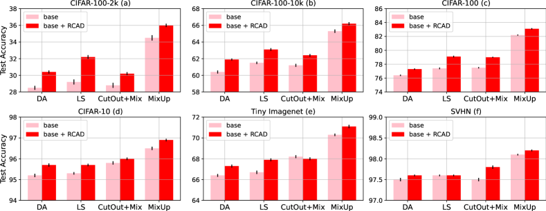
Figure 2: Main results on supervised image classification benchmarks: We plot the mean test accuracy and 95%percent9595\% confidence intervals over 101010 independent runs for models trained with base methods: Data Augmentation (DA), Label Smoothing (LS), CutOut/CutMix (CutOut+Mix) augmentation, MixUp and compare them with the test accuracies of the models trained with the RCAD objective in Equation 2, in addition to the base methods.

4.1 How much does RCAD improve test accuracy in comparison and in addition to other regularization methods?

Figure 2 presents the main empirical findings of RCAD over six image classification benchmarks and across four baseline regularizers. Across all datasets, we observe that training with the RCAD objective improves the test accuracy over the baseline method in 22/24222422/24 cases. The effects are more pronounced on datasets with fewer training samples. For example, on CIFAR-100-2k, adding RCAD on top of label smoothing boosts the performance by 3%absentpercent3\approx 3\%. These results also show that the benefits of RCAD are complementary to prior methods—RCAD + MixUp outperforms MixUp, and RCAD + augmentation/smoothing outperforms both. We test for statistical significance using a 1-sided p𝑝p-value, finding that p1e3much-less-than𝑝1𝑒3p\ll 1e{-3} in 22/24222422/24 comparisons. In summary, these results show that our proposed regularizer is complementary to prior regularization techniques.
Refer to caption
(a)
Refer to caption
(b)
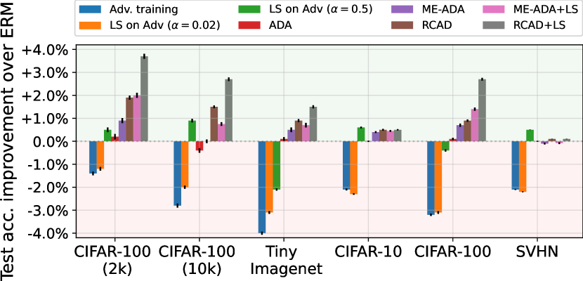
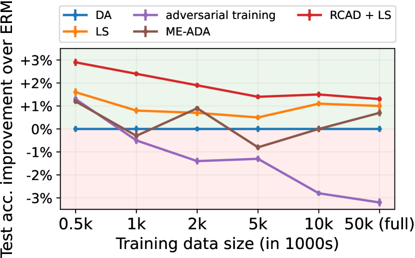
Figure 3: (Left)How should we use adversarial examples to improve test accuracy? We compare RCAD with adversarial baselines including label smoothing on adversarial samples (LS on Adv), measuring the improvement in test accuracy relative to ERM. We also compare RCAD with ME-ADA when combined with label smoothing. (Right)RCAD is more effective in low-data regime. We compare the test accuracy improvement over ERM for baselines: Label Smoothing (LS), Data Augmentation (DA), adversarial training, and ME-ADA with RCAD + LS on different sub-samples of CIFAR-100 training set (0.50.50.5k 50absent50\rightarrow 50k). We find RCAD achieves the largest gains in the low data regime. In both plots, we plot the mean and 95%percent9595\% confidence intervals over 101010 independent runs.

4.2 How effectively does RCAD improve test accuracy compared to adversarial training?

Our next set of experiments compares different ways of using adversarial examples. RCAD maximizes the model’s predictive entropy on unlabeled examples along the adversarial direction (obtained with a large step-size 0.5absent0.5\approx 0.5). In contrast, other methods we compare against (Adversarial Training [35], ADA [61], ME-ADA [61]) minimize the cross entropy loss on examples obtained by adversarially perturbing the inputs without changing the original labels (using a much smaller step size 0.05absent0.05\approx 0.05). Additionally, we look at the baseline that performs label smoothing on these adversarial samples (LS on Adv) – a relaxed version of RCAD. We evaluate all methods by measuring their test accuracy improvement over empirical risk minimization (ERM), noting that some of these methods were proposed to optimize robustness, a different metric. We show results in Figure 3(a) and note that RCAD outperforms adversarial training and LS on Adv with small step-sizes (α=0.02)𝛼0.02(\alpha=0.02), ADA and ME-ADA by significant margins on all benchmarks. We numerically verify that RCAD statistically outperforms the best baseline ME-ADA by computing 111-sided p𝑝p-values (p𝑝p=0.0090.0090.009 on CIFAR-10, p<1e4𝑝1𝑒4p<1e{-4} on others).

Next, we look at LS on Adv with large α=0.5𝛼0.5\alpha=0.5. Since this is the same value of α𝛼\alpha used by RCAD for most datasets, this method is equivalent to performing label smoothing on examples generated by RCAD. Since label smoothing is a relaxed form of entropy maximization it is not surprising that the performance of this method is similar to (if not better than) RCAD on a few benchmarks. Finally, when both RCAD and ME-ADA are equipped with label smoothing, both methods improve, but the benefit of RCAD persists (p𝑝p == 0.04780.04780.0478 on CIFAR-10, p<1e4𝑝1𝑒4p<1e{-4} on others).

4.3 How effective is RCAD in the low training data regime?

Since supervised learning methods are more susceptible to overfitting when training samples are limited [12], we analyze the effectiveness of RCAD in the low-data regime. To verify this, we sample small training datasets of size 0.5k, 1k, 2k, 5k and 10k from the 50,000 training samples in CIFAR-100. The test set for each is the same as that of CIFAR-100. We train the baseline regularizers and RCAD on each of these datasets and compare the observed improvements in test accuracies relative to ERM. We show our results for this experiment in Figure 3(b). Straight away we observe that RCAD yields positive improvements in test accuracy for any training dataset size. In contrast, in line with the robust overfitting phenomena described in Raghunathan et al., [47, 46], Zhang et al., 2019a [69], adversarial training (with FGSM [13]) is found to be hurtful in some settings. Next we observe that compared to typical regularizers for supervised learning like label smoothing and data augmentation, the regularization effect of RCAD has a stronger impact as the size of the training data reduces. Notice that RCAD has a steeper upward trend (right\rightarrowleft) compared to the next best method label smoothing, while outperforming each baseline in terms of absolute performance values.

4.4 Additional Results and Ablations

In addition to the experiments below on wider architectures, effect of step size α𝛼\alpha, and regression tasks, we conduct more analysis and experiments for RCAD (e.g., evaluating its robustness to adversarial perturbations and distribution shifts). For these and other experimental details refer to Appendix BC.

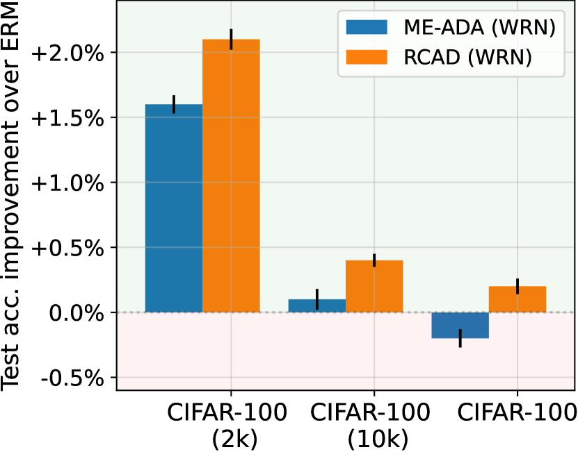
Results on a larger architecture. We compare the test accuracies of RCAD and ME-ADA (most competitive baseline from ResNet-18 experiments) when trained with the larger backbone Wide ResNet 28-10 [66] (WRN) on CIFAR-100 and its derivatives. We plot these test accuracies relative to ERM trained with WRN in Figure 4a. Clearly, the benefit of RCAD over ME-ADA still persists albeit with slightly diminished absolute performance differences compared to ResNet-18 in Figure 3(a).

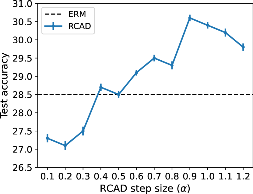
Effect of step size α𝛼\alpha on test accuracy. In Figure 4b we plot the test accuracy of RCAD on CIFAR-100-2k as we vary the step size α𝛼\alpha. We see that RCAD is effective only when the step size is sufficiently large (>0.5absent0.5>0.5), so that new examples do not resemble the original ones. When the step size is small (<0.5)absent0.5(<0.5), the perturbations are small and the new example is indistinguishable from the original, as in adversarial training. Our theory in Section 5 also agrees with this observation.

Results on regression tasks. On five regression datasets from the UCI repository we compare the performance of RCAD with ERM and ME-ADA in terms of test negative log-likelihood (NLL) (\downarrow is better). To be able to compute NLL, we model the predictive distribution p𝒘(y𝐱)subscript𝑝𝒘conditionaly𝐱p_{{\bm{w}}}({\textnormal{y}}\mid{\mathbf{x}}) as a Gaussian and each method outputs two parameters (mean, variance of p𝒘(y𝐱)subscript𝑝𝒘conditionaly𝐱p_{{\bm{w}}}({\textnormal{y}}\mid{\mathbf{x}})) at each input 𝐱𝐱{\mathbf{x}}. For the RCAD regularizer we use the differential form of entropy. Results are shown in Figure 4c from which we see that RCAD matches/improves over baselines on 4/5 regression datasets.
Refer to caption
(a)
Refer to caption
(b)
Negative log-likelihood (NLL) on test data
Method Boston Concrete Energy Wine Yacht
ERM 2.852.852.85 ±0.06plus-or-minus0.06\pm 0.06 3.253.253.25 ±0.07plus-or-minus0.07\pm 0.07 1.851.85\mathbf{1.85} ±0.03plus-or-minus0.03\pm 0.03 0.970.97\mathbf{0.97} ±0.04plus-or-minus0.04\pm 0.04 1.661.661.66 ±0.04plus-or-minus0.04\pm 0.04
ME-ADA 3.013.013.01 ±0.04plus-or-minus0.04\pm 0.04 3.143.14\mathbf{3.14} ±0.03plus-or-minus0.03\pm 0.03 1.991.991.99 ±0.06plus-or-minus0.06\pm 0.06 1.111.111.11 ±0.05plus-or-minus0.05\pm 0.05 1.781.781.78 ±0.04plus-or-minus0.04\pm 0.04
RCAD (ours) 2.602.60\mathbf{2.60} ±0.05plus-or-minus0.05\pm 0.05 3.123.12\mathbf{3.12} ±0.04plus-or-minus0.04\pm 0.04 1.751.75\mathbf{1.75} ±0.07plus-or-minus0.07\pm 0.07 1.091.091.09 ±0.05plus-or-minus0.05\pm 0.05 1.541.54\mathbf{1.54} ±0.05plus-or-minus0.05\pm 0.05
(c)
Figure 4: RCAD can be used with larger networks and is also effective on regression tasks. (Left) We compare the improvements in test accuracy (over ERM) for RCAD and ME-ADA when all methods use Wide ResNet 28-10 [66]. (Center) For CIFAR-100-2k, we show the effect on test accuracy of the step size α𝛼\alpha that RCAD takes while generating out-of-distribution examples along the adversarial direction. (Right) We compare the negative log-likelihood on test samples for RCAD with baselines ERM and ME-ADA on five regression datasets from the UCI repository. For the above we show the mean and 95%percent9595\% confidence intervals across 101010 runs.

5 Analysis: Why Does RCAD Improve Test Performance?

In this section, we present theoretical results that provide a more formal explanation as to why we see a boost in test accuracy when we regularize a classifier using RCAD. We analyze the simplified problem of learning l2subscript𝑙2l_{2}-regularized linear predictors in a fully specified binary classification setting. Specifically, our analysis will show that, while linear predictors trained with standard ERM can have a high dependence on spurious features, further optimization with the RCAD objective will cause the classifier to unlearn these spurious features.

The intuition behind our result can be summarized as follows: when RCAD generates examples after taking a large step along adversarial directions, a majority of the generated examples end up lying close to the decision boundary along the true feature, and yet a portion of them would significantly depend on the noisy spurious features. Thus, when RCAD maximizes the predictive entropy on these new examples, the classifier weights that align with the spurious components are driven toward smaller values. Detailed proofs for the analysis that follows can be found in Appendix A.

Setup.

We consider a binary classification problem with a joint distribution 𝒟𝒟{\mathcal{D}} over (𝐱,y)𝒳×{0,1}𝐱y𝒳01({\mathbf{x}},{\textnormal{y}})\in{\mathcal{X}}\times\{0,1\} where 𝒳d+1𝒳superscript𝑑1{\mathcal{X}}\subseteq\operatorname{\mathbb{R}}^{d+1} with 𝐱=[x1,𝐱2]𝐱superscriptsubscriptx1subscript𝐱2top{\mathbf{x}}=\left[{\textnormal{x}}_{1},{\mathbf{x}}_{2}\right]^{\top}, x1,𝐱2dformulae-sequencesubscriptx1subscript𝐱2superscript𝑑{\textnormal{x}}_{1}\in\operatorname{\mathbb{R}},\;{\mathbf{x}}_{2}\in\operatorname{\mathbb{R}}^{d} and for some β>0𝛽0\beta>0, 𝒟𝒟{\mathcal{D}} is:

yUnif{1,1},x1𝒩(βy,σ12),𝐱2𝒩(𝟎,Σ2),and letΣ~(σ12𝟎𝟎Σ2).formulae-sequencesimilar-toyUnif11formulae-sequencesimilar-tosubscriptx1𝒩𝛽ysuperscriptsubscript𝜎12formulae-sequencesimilar-tosubscript𝐱2𝒩0subscriptΣ2and let~Σsuperscriptsubscript𝜎1200subscriptΣ2\displaystyle{\textnormal{y}}\sim\textrm{Unif}\{-1,1\},\;\;{\textnormal{x}}_{1}\sim{\mathcal{N}}(\beta\cdot{\textnormal{y}},\sigma_{1}^{2}),\;\;{\mathbf{x}}_{2}\sim\mathcal{N}({\mathbf{0}},\Sigma_{2}),\;\;\textrm{and let}\;\;\tilde{\Sigma}\triangleq\left(\begin{array}[]{cc}\sigma_{1}^{2}&\mathbf{0}\\ \mathbf{0}&\Sigma_{2}\end{array}\right). (5)

We borrow this setup from Chen et al., 2020b [6] which analyzes self-training/entropy minimization on unlabeled out-of-distribution samples. While their objective is very different from RCAD, their setup is relevant for our analysis since it captures two kinds of features: x1subscriptx1{\textnormal{x}}_{1}, which is the true univariate feature that is predictive of the label y, and 𝐱2subscript𝐱2{\mathbf{x}}_{2}, which is the high dimensional noise, that is not correlated with the label under the true distribution 𝒟𝒟{\mathcal{D}}, but w.h.p. is correlated with the label on finite sampled training dataset 𝒟^={(𝐱(i),y(i))}i=1n𝒟n^𝒟superscriptsubscriptsuperscript𝐱𝑖superscripty𝑖𝑖1𝑛similar-tosuperscript𝒟𝑛{\hat{\mathcal{D}}}=\{({\mathbf{x}}^{(i)},{\textnormal{y}}^{(i)})\}_{i=1}^{n}\sim{\mathcal{D}}^{n}. We wish to learn the class of homogeneous linear predictors 𝒲{𝒘d+1:𝒘,𝐱=w1x1+𝒘2𝐱2,𝒘21}𝒲conditional-set𝒘superscript𝑑1formulae-sequence𝒘𝐱subscript𝑤1subscriptx1subscript𝒘2subscript𝐱2subscriptnorm𝒘21{\mathcal{W}}\triangleq\{{\bm{w}}\in\operatorname{\mathbb{R}}^{d+1}:\langle{\bm{w}},{\mathbf{x}}\rangle={w}_{1}\cdot{\textnormal{x}}_{1}+{\bm{w}}_{2}\cdot{\mathbf{x}}_{2},\left\|{\bm{w}}\right\|_{2}\leqslant 1\}. For mathematical convenience we make three modifications to the RCAD objective in Equation 2 that are common in works analyzing logistic classifiers and entropy based objectives  [54, 6]: (i) we minimize the margin loss lγ(𝒘;(𝐱,y))max(0,γy𝒘,𝐱)subscript𝑙𝛾𝒘𝐱y0𝛾y𝒘𝐱l_{\gamma}({\bm{w}};({\mathbf{x}},{\textnormal{y}}))\triangleq\max(0,\gamma-{\textnormal{y}}\cdot\langle{\bm{w}},{\mathbf{x}}\rangle) (instead of the negative log-likelihood) over 𝒟superscript𝒟{\mathcal{D}}^{\prime} with some γ>0𝛾0\gamma>0; (ii) we consider the constrained optimization problem in Equation 6 as opposed to the Lagrangian form of RCAD in Equation 2 [34]; and (iii) we use Lemma 5.1 and replace 𝒘(𝐱+α𝐱lγ(𝒘;(𝐱,y)))subscript𝒘𝐱𝛼subscript𝐱subscript𝑙𝛾𝒘𝐱y{\mathcal{H}}_{\bm{w}}({\mathbf{x}}+\alpha\cdot\nabla_{{\mathbf{x}}}l_{\gamma}({\bm{w}};({\mathbf{x}},{\textnormal{y}}))) with exp(|𝒘,𝐱+α𝐱lγ(𝒘;(𝐱,y))|)𝒘𝐱𝛼subscript𝐱subscript𝑙𝛾𝒘𝐱y\exp(-|\langle{\bm{w}},{\mathbf{x}}+\alpha\cdot\nabla_{{\mathbf{x}}}l_{\gamma}({\bm{w}};({\mathbf{x}},{\textnormal{y}}))\rangle|). Note that the optimal 𝒘𝒲superscript𝒘𝒲{\bm{w}}^{*}\in{\mathcal{W}} that has the best test accuracy and lowest population margin loss is given by 𝒘[1,0,,0]superscript𝒘superscript100top{\bm{w}}^{*}\triangleq\left[1,0,\dots,0\right]^{\top}.

max𝒘𝒟^(𝒘)𝔼𝒟^exp(|𝒘,𝐱+α𝒙lγ(𝒘;(𝐱,y))|)subscript𝒘subscript^𝒟𝒘subscript𝔼^𝒟𝒘𝐱𝛼subscript𝒙subscript𝑙𝛾𝒘𝐱y\displaystyle\max_{{\bm{w}}}\;\;{\mathcal{M}}_{\hat{\mathcal{D}}}({\bm{w}})\triangleq\mathbb{E}_{\hat{{\mathcal{D}}}}\;\exp(-|\langle{\bm{w}},{\mathbf{x}}+\alpha\cdot\nabla_{{\bm{x}}}l_{\gamma}({\bm{w}};({\mathbf{x}},{\textnormal{y}}))\rangle|)
s.t.𝔼𝒟^ 1(lγ(𝒘;(𝐱,y))>0)ρ/2,𝒘𝒲formulae-sequences.t.subscript𝔼^𝒟1subscript𝑙𝛾𝒘𝐱y0𝜌2𝒘𝒲\displaystyle\;\,\textrm{s.t.}\;\;\;\;\mathbb{E}_{\hat{\mathcal{D}}}\;\mathbbm{1}(l_{\gamma}({\bm{w}};({\mathbf{x}},{\textnormal{y}}))>0)\leqslant\rho/2,\;\;{\bm{w}}\in{\mathcal{W}} (6)
Lemma 5.1 ([5, 54], informal).

𝒘(𝐱)=bin((1+exp(𝒘,𝐱))1)subscript𝒘𝐱subscriptbinsuperscript1𝒘𝐱1{\mathcal{H}}_{\bm{w}}({\mathbf{x}})={\mathcal{H}}_{\mathrm{bin}}((1+\exp(-\langle{\bm{w}},{\mathbf{x}}\rangle))^{-1}) where bin(p)subscriptbin𝑝{\mathcal{H}}_{\mathrm{bin}}(p) is the entropy of Bern(p)Bern𝑝\operatorname{\mathrm{Bern}}(p) distribution. Thus 𝐰(𝐱)exp(|𝐰,𝐱|)subscript𝐰𝐱𝐰𝐱{\mathcal{H}}_{\bm{w}}({\mathbf{x}})\approx\exp(-|\langle{\bm{w}},{\mathbf{x}}\rangle|), as both exhibit same tail behavior.

We analyze the RCAD estimate 𝒘^rcad𝒘(T)subscript^𝒘rcadsuperscript𝒘𝑇\hat{{\bm{w}}}_{\mathrm{rcad}}\triangleq{{\bm{w}}^{(T)}} returned after T𝑇T iterations of projected gradient ascent on the non-convex objective in Equation 6, initialized with 𝒘(0)superscript𝒘0{{\bm{w}}^{(0)}} satisfying the constraints in Equation 6. Given the projection Π𝒮subscriptΠ𝒮\Pi_{\mathcal{S}} onto the convex set 𝒮𝒮{\mathcal{S}}, and learning rate η>0𝜂0\eta>0, the update rule for 𝒘(t)superscript𝒘𝑡{{\bm{w}}^{(t)}} is as follows: 𝒘~(t+1)=𝒘(t)+η𝒘(t)𝒟^(𝒘)superscript~𝒘𝑡1superscript𝒘𝑡𝜂subscriptsuperscript𝒘𝑡subscript^𝒟𝒘\tilde{{\bm{w}}}^{(t+1)}={{\bm{w}}^{(t)}}+\eta\cdot\nabla_{{{\bm{w}}^{(t)}}}{\mathcal{M}}_{\hat{\mathcal{D}}}({\bm{w}}), and 𝒘(t+1)=Π𝒘21𝒘~(t+1)superscript𝒘𝑡1subscriptΠsubscriptnorm𝒘21superscript~𝒘𝑡1{{\bm{w}}^{(t+1)}}=\Pi_{\|{\bm{w}}\|_{2}\leqslant 1}\tilde{{\bm{w}}}^{(t+1)}. Since the initialization 𝒘(0)superscript𝒘0{{\bm{w}}^{(0)}} satisfies the constraint in Equation 6, it has a low margin loss on training samples and using margin based generalization gaps [26] we can conclude w.h.p. 𝒘(0)superscript𝒘0{{\bm{w}}^{(0)}} has low test error (ρ)absent𝜌(\leqslant\rho). This, in turn tells us that 𝒘(0)superscript𝒘0{{\bm{w}}^{(0)}} should have learnt the true feature x1subscript𝑥1x_{1} to some extent (Lemma 5.2). Intuitively, if the classifier is not trained at all, then adversarial directions would be less meaningful since they may include a higher component of the true feature x1subscriptx1{\textnormal{x}}_{1}, as opposed to noisy 𝐱2subscript𝐱2{\mathbf{x}}_{2}. To obtain 𝒘(0)superscript𝒘0{{\bm{w}}^{(0)}}, we simply minimize loss lγsubscript𝑙𝛾l_{\gamma} on 𝒟^^𝒟\hat{\mathcal{D}} using projected (onto 𝒘21subscriptnorm𝒘21\|{\bm{w}}\|_{2}\leqslant 1) gradient descent and the ERM solution 𝒘^ermsubscript^𝒘erm\hat{{\bm{w}}}_{\mathrm{erm}} serves as the initialization 𝒘(0)superscript𝒘0{{\bm{w}}^{(0)}} for RCAD’s gradient ascent iterations. Note that 𝒘^ermsubscript^𝒘erm\hat{{\bm{w}}}_{\mathrm{erm}} still significantly depends on spurious features (see Figure 5). Furthermore, this dependence is unavoidable and worse when n𝑛n is small, or when the noise dimension d𝑑d is large.

Refer to caption
(a)
Refer to caption
(b)
Refer to caption
(c)
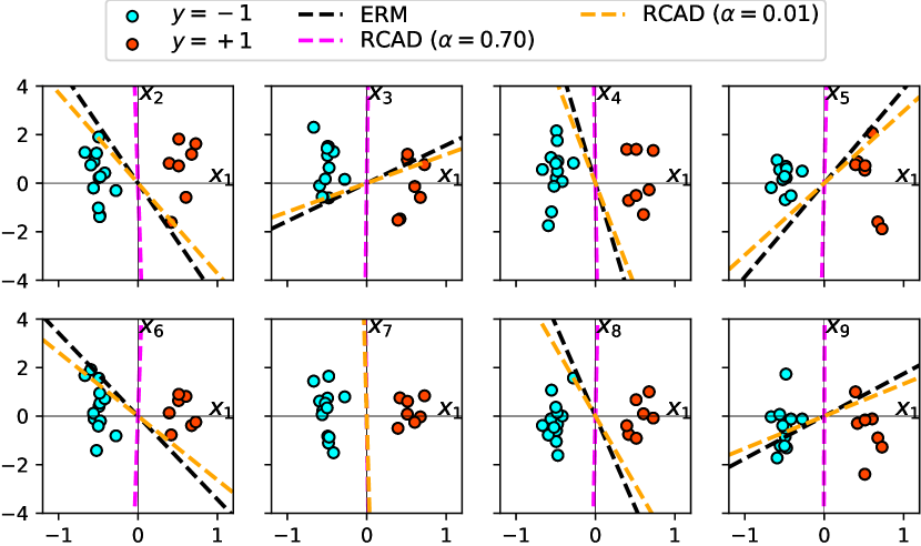
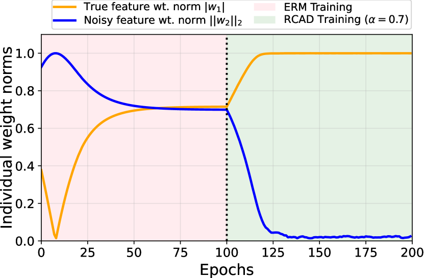
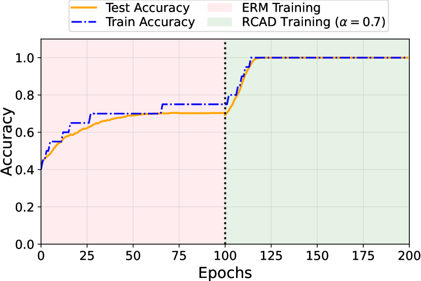
Figure 5: RCAD corrects ERM solution: (Left)  We plot the training data and high-dimensional decision boundaries for all three estimates 𝒘^ermsubscript^𝒘erm\hat{{\bm{w}}}_{\mathrm{erm}} and 𝒘^rcadsubscript^𝒘rcad\hat{{\bm{w}}}_{\mathrm{rcad}} with α=0.01,0.70𝛼0.010.70\alpha=0.01,0.70. Here, we plot the linear boundary projected onto the set of planes {x1,xi}i=2i=8superscriptsubscriptsubscriptx1subscriptx𝑖𝑖2𝑖8\{{\textnormal{x}}_{1},{\textnormal{x}}_{i}\}_{i=2}^{i=8} spanned by the true feature x1subscriptx1{\textnormal{x}}_{1} and noisy features x2,,x8subscriptx2subscriptx8{\textnormal{x}}_{2},\ldots,{\textnormal{x}}_{8}. Across the ERM and RCAD training iterations, we plot the weight norms along the true feature |w1|subscript𝑤1|{w}_{1}| and noisy dimensions 𝒘22subscriptnormsubscript𝒘22\|{\bm{w}}_{2}\|_{2} in the (Center) plot, and on the (Right) we plot the train/test accuracies.
Lemma 5.2 (true feature is partially learnt before RCAD).

If 𝐰(0)superscript𝐰0{{\bm{w}}^{(0)}} satisfies constraint in  Equation 6, and when n  > [-0.07cm] β2+log(1/δ)Σ~op+Σ~γ2ρ2𝑛  > [-0.07cm] superscript𝛽21𝛿subscriptnorm~Σopsubscriptnorm~Σsuperscript𝛾2superscript𝜌2n\raisebox{-3.69899pt}{~{}\shortstack{$>$ \\ [-0.07cm] $\sim$}}~{}\frac{\beta^{2}+\log(1/\delta)\cdot\|\tilde{\Sigma}\|_{\mathrm{op}}+\|\tilde{\Sigma}\|_{*}}{\gamma^{2}\rho^{2}}, with probability 1δ1𝛿1-\delta over 𝒟^^𝒟\hat{{\mathcal{D}}}, w1(0)erfc1(2ρ)2σmin(Σ~)βsubscriptsuperscript𝑤01superscripterfc12𝜌2subscript𝜎min~Σ𝛽\;\;{{w}^{(0)}_{1}}\geqslant\frac{\mathrm{erfc}^{-1}\left(2\rho\right)\cdot\sqrt{2\sigma_{\mathrm{min}}(\tilde{\Sigma})}}{\beta}.

We are now ready to present our main results in Theorem 5.3 which states that after T=𝒪(log(1/ϵ))𝑇𝒪1italic-ϵT={\mathcal{O}}(\log(1/\epsilon)) gradient ascent iterations of optimizing the RCAD objective 𝒘^rcadsubscript^𝒘rcad{\hat{{\bm{w}}}}_{\mathrm{rcad}} is ϵitalic-ϵ\epsilon close to 𝒘superscript𝒘{\bm{w}}^{*}, since it unlearns the spurious feature (𝒘2(T)2ϵ)subscriptnormsubscriptsuperscript𝒘𝑇22italic-ϵ(\|{{\bm{w}}^{(T)}_{2}}\|_{2}\leqslant\epsilon) and amplifies the true feature (|w1(T)|1ϵ2)subscriptsuperscript𝑤𝑇11superscriptitalic-ϵ2(|{{w}^{(T)}_{1}}|\geqslant\sqrt{1-\epsilon^{2}}). Note that Theorem 5.3 suggests a minimum step size α𝛼\alpha in arriving at a sufficient condition for RCAD to unlearn spuriousness and improve test performance This is also in line with our empirical findings (Figure 4b). Since α=Θ(γ)𝛼Θ𝛾\alpha=\Theta(\gamma), most of the points generated by RCAD lie close to the decision boundary along x1subscriptx1{\textnormal{x}}_{1}, except for the ones with noisy features that are correlated with the classifier weights.

Theorem 5.3 (𝒘^rcad𝒘subscript^𝒘rcadsuperscript𝒘\hat{{\bm{w}}}_{\mathrm{rcad}}\rightarrow{\bm{w}}^{*}).

If β=Ω(Σ~op)𝛽Ωsubscriptnorm~Σop\beta=\Omega(\|\tilde{\Sigma}\|_{\mathrm{op}}) and c0,K>0subscript𝑐0𝐾0\exists\;c_{0},K>0, such that β  > [-0.07cm] α  > [-0.07cm] max(γ,Σ~op)𝛽  > [-0.07cm] 𝛼  > [-0.07cm] 𝛾subscriptnorm~Σop\beta\raisebox{-3.69899pt}{~{}\shortstack{$>$ \\ [-0.07cm] $\sim$}}~{}\alpha\raisebox{-3.69899pt}{~{}\shortstack{$>$ \\ [-0.07cm] $\sim$}}~{}\max(\gamma,\|\tilde{\Sigma}\|_{\mathrm{op}}) and γ+c0σmin(Σ~)β𝛾subscript𝑐0subscript𝜎min~Σ𝛽\gamma+c_{0}\cdot\sigma_{\mathrm{min}}(\tilde{\Sigma})\geqslant\beta, then with n  > [-0.07cm] β2+log(1/δ)Σ~op+Σ~γ2erfc(Kα/2σmin(Σ~))2+log1/δϵ4𝑛  > [-0.07cm] superscript𝛽21𝛿subscriptnorm~Σopsubscriptnorm~Σsuperscript𝛾2erfcsuperscript𝐾𝛼2subscript𝜎min~Σ21𝛿superscriptitalic-ϵ4n\raisebox{-3.69899pt}{~{}\shortstack{$>$ \\ [-0.07cm] $\sim$}}~{}\frac{\beta^{2}+\log(1/\delta)\cdot\|\tilde{\Sigma}\|_{\mathrm{op}}+\|\tilde{\Sigma}\|_{*}}{\gamma^{2}\mathrm{erfc}\left(K\alpha/\sqrt{2\sigma_{\mathrm{min}}(\tilde{\Sigma})}\right)^{2}}+\frac{\log{1/\delta}}{\epsilon^{4}}, after T=𝒪(log(1/ϵ))𝑇𝒪1italic-ϵT={\mathcal{O}}\left(\log(1/\epsilon)\right) gradient ascent iterations, |w1(T)|1ϵ2subscriptsuperscript𝑤𝑇11superscriptitalic-ϵ2|{{w}^{(T)}_{1}}|\geqslant\sqrt{1-\epsilon^{2}} and 𝐰2(T)2ϵsubscriptnormsubscriptsuperscript𝐰𝑇22italic-ϵ\|{{{\bm{w}}^{(T)}_{2}}}\|_{2}\leqslant\epsilon, with probability 1δ1𝛿1-\delta over 𝒟superscript𝒟\mathcal{D}^{\prime}.

The key idea behind our guarantee above is an inductive argument. We show that, if the class separation β𝛽\beta and step size α𝛼\alpha are sufficiently larger than any noise variance, then RCAD monotonically increases the weight norm along the true feature and monotonically decreases it along the noisy dimensions with each gradient ascent update. This is because at any given instant the gradient of RCAD objective 𝒟(𝒘)subscript𝒟𝒘{\mathcal{M}}_{\mathcal{D}}({\bm{w}}) with respect to w1subscript𝑤1{w}_{1} always points in the same direction, while the one with respect to 𝒘2subscript𝒘2{\bm{w}}_{2} is sufficiently anti-correlated with the direction of 𝒘2subscript𝒘2{\bm{w}}_{2}. We formalize this argument in Lemma 5.4. It is also easy to see why the update will improve test accuracy monotonically, thus satisfying the constraint in Equation 6 with high probability.

Lemma 5.4 (w1,𝒘2subscript𝑤1subscript𝒘2{w}_{1},{\bm{w}}_{2} update).

If α,β,γ𝛼𝛽𝛾\alpha,\beta,\gamma and sample size n𝑛n satisfy the noise conditions in Theorem 5.3, then 𝒟(𝐰)w1(t),w1(t)>0subscript𝒟𝐰subscriptsuperscript𝑤𝑡1subscriptsuperscript𝑤𝑡10\langle\frac{\partial{\mathcal{M}}_{\mathcal{D}}({\bm{w}})}{\partial{{w}^{(t)}_{1}}},{{w}^{(t)}_{1}}\rangle>0, and |w~1(t+1)|>|w1(t)|subscriptsuperscript~𝑤𝑡11subscriptsuperscript𝑤𝑡1|{\tilde{{w}}^{(t+1)}_{1}}|>|{{w}^{(t)}_{1}}|. On the other hand, c1>0subscript𝑐10\exists c_{1}>0 such that 𝐰2(t)𝒟(𝐰(t)),𝐰2(t)c1𝐰2(t)22subscriptsubscriptsuperscript𝐰𝑡2subscript𝒟superscript𝐰𝑡subscriptsuperscript𝐰𝑡2subscript𝑐1superscriptsubscriptnormsubscriptsuperscript𝐰𝑡222\langle\nabla_{{{\bm{w}}^{(t)}_{2}}}{{\mathcal{M}}_{\mathcal{D}}({{\bm{w}}^{(t)}})},{{\bm{w}}^{(t)}_{2}}\rangle\leqslant-c_{1}\cdot\|{{\bm{w}}^{(t)}_{2}}\|_{2}^{2}. Consequently η𝜂\exists\eta, such that 𝐰~2(t+1)2/𝐰2(t)2<1subscriptnormsubscriptsuperscript~𝐰𝑡122subscriptnormsubscriptsuperscript𝐰𝑡221\|{\tilde{{\bm{w}}}^{(t+1)}_{2}}\|_{2}/\|{{\bm{w}}^{(t)}_{2}}\|_{2}<1.

Empirically validating our theoretical results in the toy setup. Now, using the same setup as our theoretical study, we check if taking the ERM solution and updating it with RCAD truly helps in unlearning the spurious feature 𝐱2subscript𝐱2{\mathbf{x}}_{2} and amplifying the true feature x1subscriptx1{\textnormal{x}}_{1}. With d=8,γ=2.0,β=0.5,σ1=0.1,Σ=𝐈dformulae-sequence𝑑8formulae-sequence𝛾2.0formulae-sequence𝛽0.5formulae-sequencesubscript𝜎10.1Σsubscript𝐈𝑑d=8,\gamma=2.0,\beta=0.5,\sigma_{1}=0.1,\Sigma=\mathbf{I}_{d} we collect training dataset 𝒟^^𝒟\hat{\mathcal{D}} of size 202020 according to the data distribution in Equation 5. First, we obtain the ERM solution 𝒘^ermsubscript^𝒘erm\hat{{\bm{w}}}_{\mathrm{erm}} by optimizing the margin loss on 𝒟^^𝒟\hat{\mathcal{D}} for 100100100 projected gradient descent iterations. Then, with 𝒘^ermsubscript^𝒘erm\hat{{\bm{w}}}_{\mathrm{erm}} as initialization we optimize the RCAD objective in Equation 6 for 100100100 additional projected gradient ascent iterations to obtain RCAD estimate 𝒘^rcadsubscript^𝒘rcad\hat{{\bm{w}}}_{\mathrm{rcad}}. For RCAD, we try both small (α=0.01)𝛼0.01(\alpha=0.01) and large (α=0.7)𝛼0.7(\alpha=0.7) values of the step size. Using the results of this study in Figure 5 we shall now verify our main theoretical claims:

(i) RCAD unlearns spurious features learnt by ERM (Theorem 5.3): RCAD training with large step size α=0.7𝛼0.7\alpha=0.7 corrects ERM’s decision boundaries across all noisy dimensions i.e., 𝒘^rcadsubscript^𝒘rcad\hat{{\bm{w}}}_{\mathrm{rcad}} has almost no dependence on noisy dimensions {xi}i=2i=8superscriptsubscriptsubscriptx𝑖𝑖2𝑖8\{{\textnormal{x}}_{i}\}_{i=2}^{i=8} (Figure 5(a)). On the other hand, the ERM solution has a significant non-zero component across all noisy dimensions (except x7subscriptx7{\textnormal{x}}_{7}).

(ii) RCAD is helpful only when step size is large enough (Theorem 5.3): In Figure 5(a) we see that RCAD estimate with small step size α=0.01𝛼0.01\alpha=0.01 has a higher dependence on spurious features compared to ERM. Thus optimizing RCAD with a very small α𝛼\alpha leads to an even poor solution than ERM. This is because, the perturbed data point still has a significant component of the true feature, which the model is forced to unlearn when RCAD tries to maximize entropy over the perturbed point.

(iii) The weight norms |w1|subscript𝑤1|{w}_{1}| and w22subscriptnormsubscript𝑤22\|{\bm{w}}_{2}\|_{2} change monotonically through RCAD iterations (Lemma 5.4): In Figure 5(b) we see that the norm along the true feature |w1|subscript𝑤1|{w}_{1}| increases monotonically through RCAD iterations, whereas 𝒘22subscriptnormsubscript𝒘22\|{\bm{w}}_{2}\|_{2} decreases monotonically, until |w1|1subscript𝑤11|{w}_{1}|\approx 1 and 𝒘220subscriptnormsubscript𝒘220\|{\bm{w}}_{2}\|_{2}\approx 0. Thus, RCAD successfully recovers optimal 𝒘superscript𝒘{\bm{w}}^{*}. Based on this, we also see the test accuracy increase monotonically through RCAD iterations; reaching 100%percent100100\% by the end of it (Figure 5(c)). In contrast, since the ERM solution depends on spurious features, its accuracy does not improve beyond 70%percent7070\% in the first 100100100 iterations. We find that training ERM for more iterations only improves training accuracy.

The analysis above explains why RCAD improves test performance in the linear setting and it is inline with our intuition of RCAD’s ability to unlearn spurious features. To check if our intuition also generalizes to deeper networks we further study RCAD’s behaviour in a non-linear setting using a different toy example in Appendix D. Furthermore, while our analysis is restricted to linear classifiers, linear models can provide a rough proxy for neural network learning dynamics via the neural tangent kernel (NTK) approximation [23]. This strategy has been used in a number of prior works [39, 57, 2] and extending the analysis to the NTK setting may be possible in future work.

6 Conclusion

In this paper we propose RCAD, a regularization technique that maximizes a model’s predictive entropy on out-of-distribution examples. These samples lie along the directions that adversarially maximize the loss locally around the training points. Our experiments on image classification benchmarks show that RCAD not only improves test accuracy by a significant margin, but that it can also seamlessly compose with prior regularization methods. We find that RCAD is particularly effective when learning from limited data. Finally, we present analyses in a simplified setting to show that RCAD can help the model unlearn noisy features. Some current limitations of our work are that RCAD slows training by 30%percent3030\% and our theoretical analysis is limited to the linear case, which would be interesting directions to address/expand on in future work—particularly in light of the significant empirical benefits of RCAD for improving generalization.

Acknowledgements. The authors would like to thank Oscar Li, Ziyu Liu, Saurabh Garg at Carnegie Mellon University and members of the RAIL lab at UC Berkeley for helpful feedback and discussion.

References

  • Arjovsky et al., [2020] Arjovsky, M., Bottou, L., Gulrajani, I., and Lopez-Paz, D. (2020). Invariant risk minimization. stat, 1050:27.
  • Cao and Gu, [2019] Cao, Y. and Gu, Q. (2019). Generalization bounds of stochastic gradient descent for wide and deep neural networks. Advances in neural information processing systems, 32.
  • Carlini et al., [2019] Carlini, N., Athalye, A., Papernot, N., Brendel, W., Rauber, J., Tsipras, D., Goodfellow, I., Madry, A., and Kurakin, A. (2019). On evaluating adversarial robustness. arXiv preprint arXiv:1902.06705.
  • Carlini and Wagner, [2017] Carlini, N. and Wagner, D. (2017). Towards evaluating the robustness of neural networks. In 2017 ieee symposium on security and privacy (sp), pages 39–57. IEEE.
  • [5] Chen, T., Zhang, Z., Liu, S., Chang, S., and Wang, Z. (2020a). Robust overfitting may be mitigated by properly learned smoothening. In International Conference on Learning Representations.
  • [6] Chen, Y., Wei, C., Kumar, A., and Ma, T. (2020b). Self-training avoids using spurious features under domain shift. Advances in Neural Information Processing Systems, 33:21061–21071.
  • Church and Gale, [1991] Church, K. W. and Gale, W. A. (1991). A comparison of the enhanced good-turing and deleted estimation methods for estimating probabilities of english bigrams. Computer Speech & Language, 5(1):19–54.
  • Deng et al., [2009] Deng, J., Dong, W., Socher, R., Li, L.-J., Li, K., and Fei-Fei, L. (2009). Imagenet: A large-scale hierarchical image database. In 2009 IEEE conference on computer vision and pattern recognition, pages 248–255. Ieee.
  • DeVries and Taylor, [2017] DeVries, T. and Taylor, G. W. (2017). Improved regularization of convolutional neural networks with cutout. arXiv preprint arXiv:1708.04552.
  • Dubey et al., [2018] Dubey, A., Gupta, O., Raskar, R., and Naik, N. (2018). Maximum-entropy fine grained classification. Advances in neural information processing systems, 31.
  • Gao et al., [2020] Gao, Y., Wang, W., Herold, C., Yang, Z., and Ney, H. (2020). Towards a better understanding of label smoothing in neural machine translation. In Proceedings of the 1st Conference of the Asia-Pacific Chapter of the Association for Computational Linguistics and the 10th International Joint Conference on Natural Language Processing, pages 212–223.
  • Goodfellow et al., [2016] Goodfellow, I., Bengio, Y., and Courville, A. (2016). Deep learning. MIT press.
  • Goodfellow et al., [2014] Goodfellow, I. J., Shlens, J., and Szegedy, C. (2014). Explaining and harnessing adversarial examples. arXiv preprint arXiv:1412.6572.
  • Grandvalet and Bengio, [2004] Grandvalet, Y. and Bengio, Y. (2004). Semi-supervised learning by entropy minimization. Advances in neural information processing systems, 17.
  • Grathwohl et al., [2019] Grathwohl, W., Wang, K.-C., Jacobsen, J.-H., Duvenaud, D., Norouzi, M., and Swersky, K. (2019). Your classifier is secretly an energy based model and you should treat it like one. arXiv preprint arXiv:1912.03263.
  • Haarnoja et al., [2018] Haarnoja, T., Zhou, A., Abbeel, P., and Levine, S. (2018). Soft actor-critic: Off-policy maximum entropy deep reinforcement learning with a stochastic actor. In International conference on machine learning, pages 1861–1870. PMLR.
  • Hardt et al., [2016] Hardt, M., Recht, B., and Singer, Y. (2016). Train faster, generalize better: Stability of stochastic gradient descent. In International Conference on Machine Learning, pages 1225–1234. PMLR.
  • He et al., [2016] He, K., Zhang, X., Ren, S., and Sun, J. (2016). Deep residual learning for image recognition. In Proceedings of the IEEE conference on computer vision and pattern recognition, pages 770–778.
  • Heinze-Deml and Meinshausen, [2017] Heinze-Deml, C. and Meinshausen, N. (2017). Conditional variance penalties and domain shift robustness. arXiv preprint arXiv:1710.11469.
  • Hendrycks and Dietterich, [2019] Hendrycks, D. and Dietterich, T. (2019). Benchmarking neural network robustness to common corruptions and perturbations. arXiv preprint arXiv:1903.12261.
  • Hertz et al., [2018] Hertz, J., Krogh, A., and Palmer, R. G. (2018). Introduction to the theory of neural computation. CRC Press.
  • Ilyas et al., [2019] Ilyas, A., Santurkar, S., Tsipras, D., Engstrom, L., Tran, B., and Madry, A. (2019). Adversarial examples are not bugs, they are features. Advances in neural information processing systems, 32.
  • Jacot et al., [2018] Jacot, A., Gabriel, F., and Hongler, C. (2018). Neural tangent kernel: Convergence and generalization in neural networks. Advances in neural information processing systems, 31.
  • Jaynes, [1957] Jaynes, E. T. (1957). Information theory and statistical mechanics. Physical review, 106(4):620.
  • Johnson, [1932] Johnson, W. E. (1932). Probability: The deductive and inductive problems. Mind, 41(164):409–423.
  • Kakade et al., [2008] Kakade, S. M., Sridharan, K., and Tewari, A. (2008). On the complexity of linear prediction: Risk bounds, margin bounds, and regularization. Advances in neural information processing systems, 21.
  • Kalimeris et al., [2019] Kalimeris, D., Kaplun, G., Nakkiran, P., Edelman, B., Yang, T., Barak, B., and Zhang, H. (2019). Sgd on neural networks learns functions of increasing complexity. Advances in Neural Information Processing Systems, 32:3496–3506.
  • Koltchinskii and Panchenko, [2002] Koltchinskii, V. and Panchenko, D. (2002). Empirical margin distributions and bounding the generalization error of combined classifiers. The Annals of Statistics, 30(1):1–50.
  • Krizhevsky et al., [2009] Krizhevsky, A. et al. (2009). Learning multiple layers of features from tiny images. Citeseer.
  • Krogh and Hertz, [1992] Krogh, A. and Hertz, J. A. (1992). A simple weight decay can improve generalization. In Advances in neural information processing systems, pages 950–957.
  • Kschischang, [2017] Kschischang, F. R. (2017). The complementary error function. Online, April.
  • Kurakin et al., [2016] Kurakin, A., Goodfellow, I., and Bengio, S. (2016). Adversarial machine learning at scale. arXiv preprint arXiv:1611.01236.
  • Le and Yang, [2015] Le, Y. and Yang, X. (2015). Tiny imagenet visual recognition challenge. CS 231N, 7(7):3.
  • Li, [1995] Li, D. (1995). Zero duality gap for a class of nonconvex optimization problems. Journal of Optimization Theory and Applications, 85(2):309–324.
  • Madry et al., [2017] Madry, A., Makelov, A., Schmidt, L., Tsipras, D., and Vladu, A. (2017). Towards deep learning models resistant to adversarial attacks. arXiv preprint arXiv:1706.06083.
  • Miyato et al., [2018] Miyato, T., Maeda, S.-i., Koyama, M., and Ishii, S. (2018). Virtual adversarial training: a regularization method for supervised and semi-supervised learning. IEEE transactions on pattern analysis and machine intelligence, 41(8):1979–1993.
  • Moosavi-Dezfooli et al., [2016] Moosavi-Dezfooli, S.-M., Fawzi, A., and Frossard, P. (2016). Deepfool: a simple and accurate method to fool deep neural networks. In Proceedings of the IEEE conference on computer vision and pattern recognition, pages 2574–2582.
  • Müller et al., [2019] Müller, R., Kornblith, S., and Hinton, G. (2019). When does label smoothing help? arXiv preprint arXiv:1906.02629.
  • Nagarajan and Kolter, [2019] Nagarajan, V. and Kolter, J. Z. (2019). Uniform convergence may be unable to explain generalization in deep learning. Advances in Neural Information Processing Systems, 32.
  • Netzer et al., [2011] Netzer, Y., Wang, T., Coates, A., Bissacco, A., Wu, B., and Ng, A. Y. (2011). Reading digits in natural images with unsupervised feature learning. Citeseer.
  • Odena, [2016] Odena, A. (2016). Semi-supervised learning with generative adversarial networks. arXiv preprint arXiv:1606.01583.
  • Pereyra et al., [2017] Pereyra, G., Tucker, G., Chorowski, J., Kaiser, Ł., and Hinton, G. (2017). Regularizing neural networks by penalizing confident output distributions. arXiv preprint arXiv:1701.06548.
  • Peters et al., [2016] Peters, J., Bühlmann, P., and Meinshausen, N. (2016). Causal inference by using invariant prediction: identification and confidence intervals. Journal of the Royal Statistical Society. Series B (Statistical Methodology), pages 947–1012.
  • Pinto et al., [2021] Pinto, F., Yang, H., Lim, S.-N., Torr, P., and Dokania, P. K. (2021). Mix-maxent: Improving accuracy and uncertainty estimates of deterministic neural networks. In NeurIPS 2021 Workshop on Distribution Shifts: Connecting Methods and Applications.
  • Poursaeed et al., [2021] Poursaeed, O., Jiang, T., Yang, H., Belongie, S., and Lim, S.-N. (2021). Robustness and generalization via generative adversarial training. In Proceedings of the IEEE/CVF International Conference on Computer Vision (ICCV), pages 15711–15720.
  • Raghunathan et al., [2020] Raghunathan, A., Xie, S. M., Yang, F., Duchi, J., and Liang, P. (2020). Understanding and mitigating the tradeoff between robustness and accuracy. In International Conference on Machine Learning, pages 7909–7919. PMLR.
  • Raghunathan et al., [2019] Raghunathan, A., Xie, S. M., Yang, F., Duchi, J. C., and Liang, P. (2019). Adversarial training can hurt generalization. arXiv preprint arXiv:1906.06032.
  • Rockafellar et al., [2000] Rockafellar, R. T., Uryasev, S., et al. (2000). Optimization of conditional value-at-risk. Journal of risk, 2:21–42.
  • Sabour et al., [2016] Sabour, S., Cao, Y., Faghri, F., and Fleet, D. J. (2016). Adversarial manipulation of deep representations. In ICLR (Poster).
  • Sagawa et al., [2020] Sagawa, S., Raghunathan, A., Koh, P. W., and Liang, P. (2020). An investigation of why overparameterization exacerbates spurious correlations. In International Conference on Machine Learning, pages 8346–8356. PMLR.
  • Saito et al., [2019] Saito, K., Kim, D., Sclaroff, S., Darrell, T., and Saenko, K. (2019). Semi-supervised domain adaptation via minimax entropy. In Proceedings of the IEEE/CVF International Conference on Computer Vision, pages 8050–8058.
  • Shorten and Khoshgoftaar, [2019] Shorten, C. and Khoshgoftaar, T. M. (2019). A survey on image data augmentation for deep learning. Journal of Big Data, 6(1):1–48.
  • Singla and Feizi, [2021] Singla, S. and Feizi, S. (2021). Salient imagenet: How to discover spurious features in deep learning? In International Conference on Learning Representations.
  • Soudry et al., [2018] Soudry, D., Hoffer, E., Nacson, M. S., Gunasekar, S., and Srebro, N. (2018). The implicit bias of gradient descent on separable data. The Journal of Machine Learning Research, 19(1):2822–2878.
  • Szegedy et al., [2016] Szegedy, C., Vanhoucke, V., Ioffe, S., Shlens, J., and Wojna, Z. (2016). Rethinking the inception architecture for computer vision. In Proceedings of the IEEE conference on computer vision and pattern recognition, pages 2818–2826.
  • Tamar et al., [2015] Tamar, A., Glassner, Y., and Mannor, S. (2015). Optimizing the cvar via sampling. In Twenty-Ninth AAAI Conference on Artificial Intelligence.
  • Tancik et al., [2020] Tancik, M., Srinivasan, P., Mildenhall, B., Fridovich-Keil, S., Raghavan, N., Singhal, U., Ramamoorthi, R., Barron, J., and Ng, R. (2020). Fourier features let networks learn high frequency functions in low dimensional domains. Advances in Neural Information Processing Systems, 33:7537–7547.
  • Tibshirani, [1996] Tibshirani, R. (1996). Regression shrinkage and selection via the lasso. Journal of the Royal Statistical Society: Series B (Methodological), 58(1):267–288.
  • Tsipras et al., [2018] Tsipras, D., Santurkar, S., Engstrom, L., Turner, A., and Madry, A. (2018). Robustness may be at odds with accuracy. arXiv preprint arXiv:1805.12152.
  • Tsipras et al., [2019] Tsipras, D., Santurkar, S., Engstrom, L., Turner, A., and Madry, A. (2019). Robustness may be at odds with accuracy. arXiv: Machine Learning.
  • Volpi et al., [2018] Volpi, R., Namkoong, H., Sener, O., Duchi, J., Murino, V., and Savarese, S. (2018). Generalizing to unseen domains via adversarial data augmentation. arXiv preprint arXiv:1805.12018.
  • Wainwright, [2019] Wainwright, M. J. (2019). High-dimensional statistics: A non-asymptotic viewpoint, volume 48. Cambridge University Press.
  • Wang et al., [2020] Wang, D., Shelhamer, E., Liu, S., Olshausen, B., and Darrell, T. (2020). Tent: Fully test-time adaptation by entropy minimization. arXiv preprint arXiv:2006.10726.
  • Wang et al., [2013] Wang, X., Jiang, Y., Huang, M., and Zhang, H. (2013). Robust variable selection with exponential squared loss. Journal of the American Statistical Association, 108(502):632–643.
  • Yun et al., [2019] Yun, S., Han, D., Oh, S. J., Chun, S., Choe, J., and Yoo, Y. (2019). Cutmix: Regularization strategy to train strong classifiers with localizable features. In Proceedings of the IEEE/CVF International Conference on Computer Vision, pages 6023–6032.
  • Zagoruyko and Komodakis, [2016] Zagoruyko, S. and Komodakis, N. (2016). Wide residual networks. arXiv preprint arXiv:1605.07146.
  • [67] Zhang, C., Bengio, S., Hardt, M., Recht, B., and Vinyals, O. (2021a). Understanding deep learning (still) requires rethinking generalization. Communications of the ACM, 64(3):107–115.
  • Zhang et al., [2018] Zhang, H., Cisse, M., Dauphin, Y. N., and Lopez-Paz, D. (2018). mixup: Beyond empirical risk minimization. In International Conference on Learning Representations.
  • [69] Zhang, H., Yu, Y., Jiao, J., Xing, E., El Ghaoui, L., and Jordan, M. (2019a). Theoretically principled trade-off between robustness and accuracy. In International Conference on Machine Learning, pages 7472–7482. PMLR.
  • [70] Zhang, J., He, T., Sra, S., and Jadbabaie, A. (2019b). Why gradient clipping accelerates training: A theoretical justification for adaptivity. arXiv preprint arXiv:1905.11881.
  • [71] Zhang, Y., Gong, M., Liu, T., Niu, G., Tian, X., Han, B., Schölkopf, B., and Zhang, K. (2021b). Adversarial robustness through the lens of causality. arXiv preprint arXiv:2106.06196.
  • Zhao et al., [2020] Zhao, L., Liu, T., Peng, X., and Metaxas, D. (2020). Maximum-entropy adversarial data augmentation for improved generalization and robustness. Advances in Neural Information Processing Systems, 33:14435–14447.
  • Zhou and Levine, [2021] Zhou, A. and Levine, S. (2021). Training on test data with bayesian adaptation for covariate shift. arXiv preprint arXiv:2109.12746.

Appendix Outline

A Proofs for Section 5.

B Additional Details for Experiments in Section 4.

C RCAD can Improve Robustness to Adversarial/Natural Distribution Shifts.

D Analyzing RCAD vs. ERM in a Non-linear Toy Classification Setup.

Appendix A Proofs for Section 5

In Section 5 of the main paper we analyze the performance of our method RCAD and compare it to empirical risk minimization (ERM) in a simplified Binary classification setting. Our investigation reveals that one reason for the better test performance of RCAD could be its ability to unlearn noisy features that are spuriously correlated with the labels in the finite sampled training dataset. This is identified under some conditions over the data distribution (noise conditions) and specifically when the RCAD objective is optimized using iterations of projected gradient ascent initialized with a decent (better than random) classifier. This implies that the initial classifier (initialized with the ERM solution in our case) has learnt the true feature to some extent. The solution obtained at the end of projected gradient ascent iterations on the RCAD objective maximizing entropy along adversarial directions, is termed as the RCAD solution. We also matched some of our theoretical results to trends observed empirically with respect to both the decision boundary learnt by RCAD vs. ERM classifier and the effect of the step size α𝛼\alpha on the performance of RCAD (Figure 5).

In this section we present proofs for our theoretical claims in Section 5. For the benefit of the reader, we begin by redefining our setup with some additional notation, followed by technical details on how the new examples are generated by RCAD in this setup. We then provide an informal proof outline for our main result in Theorem 5.3.

Setup.

We consider a binary classification problem with a joint distribution 𝒟𝒟{\mathcal{D}} over (𝐱,y)𝒳×{0,1}𝐱y𝒳01({\mathbf{x}},{\textnormal{y}})\in{\mathcal{X}}\times\{0,1\} where 𝒳d+1𝒳superscript𝑑1{\mathcal{X}}\subseteq\operatorname{\mathbb{R}}^{d+1} with 𝐱=[x1,𝐱2]𝐱superscriptsubscriptx1subscript𝐱2top{\mathbf{x}}=\left[{\textnormal{x}}_{1},{\mathbf{x}}_{2}\right]^{\top}, x1,𝐱2dformulae-sequencesubscriptx1subscript𝐱2superscript𝑑{\textnormal{x}}_{1}\in\operatorname{\mathbb{R}},\;{\mathbf{x}}_{2}\in\operatorname{\mathbb{R}}^{d} and for some β>0𝛽0\beta>0, 𝒟𝒟{\mathcal{D}} is:

yUnif{1,1},x1𝒩(βy,σ12),𝐱2𝒩(𝟎,Σ2)formulae-sequencesimilar-toyUnif11formulae-sequencesimilar-tosubscriptx1𝒩𝛽ysuperscriptsubscript𝜎12similar-tosubscript𝐱2𝒩0subscriptΣ2\displaystyle{\textnormal{y}}\sim\textrm{Unif}\{-1,1\},\;\;{\textnormal{x}}_{1}\sim{\mathcal{N}}(\beta\cdot{\textnormal{y}},\sigma_{1}^{2}),\;\;{\mathbf{x}}_{2}\sim\mathcal{N}({\mathbf{0}},\Sigma_{2})
Σ~(σ12𝟎𝟎Σ2),σ𝒘𝒘TΣ~𝒘,a𝒘βw1γσ𝒘formulae-sequence~Σsuperscriptsubscript𝜎1200subscriptΣ2formulae-sequencesubscript𝜎𝒘superscript𝒘𝑇~Σ𝒘subscript𝑎𝒘𝛽subscript𝑤1𝛾subscript𝜎𝒘\displaystyle\tilde{\Sigma}\triangleq\left(\begin{array}[]{cc}\sigma_{1}^{2}&\mathbf{0}\\ \mathbf{0}&\Sigma_{2}\\ \end{array}\right),\quad\sigma_{\bm{w}}\triangleq\sqrt{{\bm{w}}^{T}\tilde{\Sigma}{\bm{w}}},\quad a_{\bm{w}}\triangleq\frac{\beta{w}_{1}-\gamma}{\sigma_{\bm{w}}} (9)

This setup is relevant for our analysis since it captures two kinds of features: x1subscriptx1{\textnormal{x}}_{1}, which is the true univariate feature that is predictive of the label y, and 𝐱2subscript𝐱2{\mathbf{x}}_{2}, which is the high dimensional noise, that is not correlated with the label under the true distribution 𝒟𝒟{\mathcal{D}}, but w.h.p. is correlated with the label on finite sampled training dataset 𝒟^={(𝐱(i),y(i))}i=1n𝒟n^𝒟superscriptsubscriptsuperscript𝐱𝑖superscripty𝑖𝑖1𝑛similar-tosuperscript𝒟𝑛{\hat{\mathcal{D}}}=\{({\mathbf{x}}^{(i)},{\textnormal{y}}^{(i)})\}_{i=1}^{n}\sim{\mathcal{D}}^{n}. We wish to learn the class of homogeneous linear predictors 𝒲{𝒘d+1:𝒘,𝐱=w1x1+𝒘2𝐱2,𝒘21}𝒲conditional-set𝒘superscript𝑑1formulae-sequence𝒘𝐱subscript𝑤1subscriptx1subscript𝒘2subscript𝐱2subscriptnorm𝒘21{\mathcal{W}}\triangleq\{{\bm{w}}\in\operatorname{\mathbb{R}}^{d+1}:\langle{\bm{w}},{\mathbf{x}}\rangle={w}_{1}\cdot{\textnormal{x}}_{1}+{\bm{w}}_{2}\cdot{\mathbf{x}}_{2},\left\|{\bm{w}}\right\|_{2}\leqslant 1\}. Following the modifications we make to the RCAD objective in Section 5, and using Lemma 5.1 we arrive at the following constrained form of the RCAD objective where lγ(𝒘;(𝐱,y))max(0,γy𝒘,𝐱)subscript𝑙𝛾𝒘𝐱y0𝛾y𝒘𝐱l_{\gamma}({\bm{w}};({\mathbf{x}},{\textnormal{y}}))\triangleq\max(0,\gamma-{\textnormal{y}}\cdot\langle{\bm{w}},{\mathbf{x}}\rangle).

max𝒘𝒟^(𝒘)𝔼𝒟^exp(|𝒘,𝐱+α𝒙lγ(𝒘;(𝐱,y))|)subscript𝒘subscript^𝒟𝒘subscript𝔼^𝒟𝒘𝐱𝛼subscript𝒙subscript𝑙𝛾𝒘𝐱y\displaystyle\max_{{\bm{w}}}\;\;{\mathcal{M}}_{\hat{\mathcal{D}}}({\bm{w}})\triangleq\mathbb{E}_{\hat{{\mathcal{D}}}}\;\exp(-|\langle{\bm{w}},{\mathbf{x}}+\alpha\cdot\nabla_{{\bm{x}}}l_{\gamma}({\bm{w}};({\mathbf{x}},{\textnormal{y}}))\rangle|)
s.t.𝔼𝒟^ 1(lγ(𝒘;(𝐱,y))>0)ρ/2,𝒘𝒲formulae-sequences.t.subscript𝔼^𝒟1subscript𝑙𝛾𝒘𝐱y0𝜌2𝒘𝒲\displaystyle\;\,\textrm{s.t.}\;\;\;\;\mathbb{E}_{\hat{\mathcal{D}}}\;\mathbbm{1}(l_{\gamma}({\bm{w}};({\mathbf{x}},{\textnormal{y}}))>0)\leqslant\rho/2,\;\;{\bm{w}}\in{\mathcal{W}} (10)

Note that the gradient 𝐱lγ(𝒘;(𝐱,y))subscript𝐱subscript𝑙𝛾𝒘𝐱y\nabla_{{\mathbf{x}}}l_{\gamma}({\bm{w}};({\mathbf{x}},{\textnormal{y}})) maybe undefined at the margins, when y𝒘,𝐱=γ𝑦𝒘𝐱𝛾y\cdot\langle{\bm{w}},{\mathbf{x}}\rangle=\gamma. Hence, we rely on subgradients defined in Equation 14. Since, many subgradient directions exist for the margin points, for consistency, we stick with 𝐱lγ(𝒘;(𝐱,y))={𝟎}subscript𝐱subscript𝑙𝛾𝒘𝐱y0\partial_{{\mathbf{x}}}l_{\gamma}({\bm{w}};({\mathbf{x}},{\textnormal{y}}))=\{\bf{0}\} when y𝒘,𝐱=γ𝑦𝒘𝐱𝛾y\cdot\langle{\bm{w}},{\mathbf{x}}\rangle=\gamma. Note, that the set of points in 𝒳𝒳{\mathcal{X}} satisfying this equality is a zero measure set. Thus, by replacing the log-likelihood loss with the margin loss and defining its gradients in this way, it is clear that RCAD would not perturb any data points lying on or beyond the margin.

𝐱lγ(𝒘;(𝐱,y))={{y𝒘}y𝒘,𝐱<γ{κy𝒘κ[0,1]}y𝒘,𝐱=γ{𝟎}otherwisesubscript𝐱subscript𝑙𝛾𝒘𝐱ycases𝑦𝒘𝑦𝒘𝐱𝛾conditional-set𝜅𝑦𝒘𝜅01𝑦𝒘𝐱𝛾0otherwise\displaystyle\partial_{{\mathbf{x}}}l_{\gamma}({\bm{w}};({\mathbf{x}},{\textnormal{y}}))=\left\{\begin{array}[]{ll}\{-y{\bm{w}}\}&\qquad y\cdot\langle{\bm{w}},{\mathbf{x}}\rangle<\gamma\\ \{-\kappa\cdot y{\bm{w}}\mid\kappa\in[0,1]\}&\qquad y\cdot\langle{\bm{w}},{\mathbf{x}}\rangle=\gamma\\ \{\mathbf{0}\}&\qquad\textrm{otherwise}\end{array}\right. (14)

The reformulated RCAD objective in Equation 10 is a non-convex optimization problem with convex constraints. Thus, different solvers may yield different solutions. The solver we choose to analyze is a typical one – taking projected gradient ascent steps to maximize the entropy term, starting from an initialization 𝒘(0)superscript𝒘0{\bm{w}}^{(0)} that satisfies the constraint in Equation 10, and one where the iterates 𝒘(t)superscript𝒘𝑡{{\bm{w}}^{(t)}} continue to do so after every projection step.

Given the projection operator Π𝒮subscriptΠ𝒮\Pi_{\mathcal{S}} onto the convex set 𝒮𝒮{\mathcal{S}}, and learning rate η>0𝜂0\eta>0, an RCAD iteration’s update rule for 𝒘(t)superscript𝒘𝑡{{\bm{w}}^{(t)}} is defined as follows:

𝒘~(t+1)superscript~𝒘𝑡1\displaystyle\tilde{{\bm{w}}}^{(t+1)} =𝒘(t)+η𝒘(t)𝒟^(𝒘(t))absentsuperscript𝒘𝑡𝜂subscriptsuperscript𝒘𝑡subscript^𝒟superscript𝒘𝑡\displaystyle={{\bm{w}}^{(t)}}+\eta\cdot\nabla_{{{\bm{w}}^{(t)}}}{\mathcal{M}}_{\hat{\mathcal{D}}}({{\bm{w}}^{(t)}})
𝒘(t+1)superscript𝒘𝑡1\displaystyle{{\bm{w}}^{(t+1)}} =Π𝒘21𝒘~(t+1)absentsubscriptΠsubscriptnorm𝒘21superscript~𝒘𝑡1\displaystyle=\Pi_{\|{\bm{w}}\|_{2}\leqslant 1}\tilde{{\bm{w}}}^{(t+1)}

Note on projection. For simplicity we shall treat the projection operation as just renormalizing 𝒘~(t+1)superscript~𝒘𝑡1\tilde{{\bm{w}}}^{(t+1)} to have unit norm, i.e.,formulae-sequence𝑖𝑒{i.e.,} 𝒘(t+1)2=1subscriptnormsuperscript𝒘𝑡121\|{{\bm{w}}}^{(t+1)}\|_{2}=1, t0for-all𝑡0\forall t\geqslant 0. This is not necessarily restrictive. In fact, the optimal solution with the lowest test error: 𝒘[1,0,,0]superscript𝒘superscript100top{\bm{w}}^{*}\triangleq\left[1,0,\dots,0\right]^{\top}, satisfies 𝒘22=1superscriptsubscriptnormsuperscript𝒘221\|{\bm{w}}^{*}\|_{2}^{2}=1, and thus lies on the boundary of 𝒲𝒲{\mathcal{W}}. Thus, we do not lose anything by renormalizing 𝒘~(t+1)superscript~𝒘𝑡1\tilde{{\bm{w}}}^{(t+1)} to get the next iterate 𝒘(t+1)superscript𝒘𝑡1{{\bm{w}}}^{(t+1)}. With this, we are ready to state an informal outline of our proof strategy.

Informal proof outline. Our main approach to prove the claim in Theorem 5.3 can be broken down and outlined in the following way:

  • Lemma A.4: First, we shall rely on typical margin based generalization bounds to show that if our training loss is low (ρ/2)absent𝜌2(\leqslant\rho/2) and training data size n𝑛n is large enough, then we can bound the test error of the ERM solution by some small value ρ𝜌\rho with high probability.

  • Lemma 5.2: Next we shall use the fact that the test error of the ERM solution is less than ρ𝜌\rho, to prove a lower bound on the true feature weights w1subscript𝑤1{w}_{1}. This tells us that the true feature has been sufficiently learned, but ERM still depends on the noisy dimensions since 𝒘220much-greater-thansubscriptnormsubscript𝒘220\|{\bm{w}}_{2}\|_{2}\gg 0, and this cannot be remedied by ERM without sampling more training data.

  • Lemma 5.4: Now, given the ERM solution as the initialization we take steps of projected gradient ascent on the reformulated RCAD objective in Equation 10. For this procedure, under some conditions on the noise terms, margin γ𝛾\gamma and step size α𝛼\alpha we show that the partial derivative of the population objective 𝒟(𝒘)subscript𝒟𝒘{\mathcal{M}}_{\mathcal{D}}({\bm{w}}) with respect w1subscript𝑤1{w}_{1} is along w1subscript𝑤1{w}_{1} at every step: 𝒟(𝒘(t))w1(t),w1(t)>0subscript𝒟superscript𝒘𝑡subscriptsuperscript𝑤𝑡1subscriptsuperscript𝑤𝑡10\langle\frac{\partial{\mathcal{M}}_{\mathcal{D}}({{\bm{w}}^{(t)}})}{\partial{{w}^{(t)}_{1}}},{{w}^{(t)}_{1}}\rangle>0. On the other hand, we show that the derivative with respect to 𝒘2subscript𝒘2{\bm{w}}_{2} is sufficiently negatively correlated with 𝒘2subscript𝒘2{\bm{w}}_{2} at every step: 𝒘2(t)𝒟(𝒘(t)),𝒘2(t)<c1𝒘2(t)22subscriptsubscriptsuperscript𝒘𝑡2subscript𝒟superscript𝒘𝑡subscriptsuperscript𝒘𝑡2subscript𝑐1superscriptsubscriptnormsubscriptsuperscript𝒘𝑡222\langle\nabla_{{\bm{w}}^{(t)}_{2}}{\mathcal{M}}_{\mathcal{D}}({{\bm{w}}^{(t)}}),{{\bm{w}}^{(t)}_{2}}\rangle<-c_{1}\cdot\|{{\bm{w}}^{(t)}_{2}}\|_{2}^{2}. Also, we note that projecting the iterates to a unit norm ball is sufficient to satisfy the constraints in Equation 10 after every ascent step.

  • Finally, we use the above two sufficient conditions to arrive at the following conclusion: RCAD gradient ascent iterations on 𝒟(𝒘)subscript𝒟𝒘{\mathcal{M}}_{\mathcal{D}}({\bm{w}}) monotonically increase the norm along the true feature (|w1(t)|)(|{{w}^{(t)}_{1}}|\uparrow) and monotonically decrease the norm along the irrelevant noisy features (𝒘2(t)2)(\|{{\bm{w}}^{(t)}_{2}}\|_{2}\downarrow), thereby unlearning the spuriousness. Next, we rely on some uniform convergence arguments from prior works [6] to show that the previous two points are true even if we approximate the population gradient 𝒘𝒟(𝒘)subscript𝒘subscript𝒟𝒘\nabla_{\bm{w}}{\mathcal{M}}_{\mathcal{D}}({\bm{w}}), with the finite sample approximation 𝒘𝒟^(𝒘)subscript𝒘subscript^𝒟𝒘\nabla_{\bm{w}}{\mathcal{M}}_{\hat{\mathcal{D}}}({\bm{w}}), yielding the high probability finite sample guarantees in Theorem 5.3.

A.1 Technical Lemmas

In this section we shall state some technical lemmas without proof, with references to works that contain the full proof. We shall use these in the following sections when proving our lemmas in Section 5.

Lemma A.1 (Lipschitz functions of Gaussians [62]).

Let X1,,Xnsubscript𝑋1subscript𝑋𝑛X_{1},\ldots,X_{n} be a vector of iid Gaussian variables and f:n:𝑓maps-tosuperscript𝑛f:\operatorname{\mathbb{R}}^{n}\mapsto\operatorname{\mathbb{R}} be L𝐿L-Lipschitz with respect to the Euclidean norm. Then the random variable f(X)𝔼[f(X)]𝑓𝑋𝔼delimited-[]𝑓𝑋f(X)-\mathbb{E}[f(X)] is sub-Gaussian with parameter at most L𝐿L, thus:

[|f(X)𝔼[f(X)]|t]2exp(t22L2),t0.formulae-sequence𝑓𝑋𝔼delimited-[]𝑓𝑋𝑡2superscript𝑡22superscript𝐿2for-all𝑡0\displaystyle\operatorname{\mathbb{P}}[|f(X)-\mathbb{E}[f(X)]|\geqslant t]\leqslant 2\cdot\exp{\left(-\frac{t^{2}}{2L^{2}}\right)},\;\;\forall\,t\geqslant 0.
Lemma A.2 (Hoeffding bound [62]).

Let X1,,Xnsubscript𝑋1subscript𝑋𝑛X_{1},\ldots,X_{n} be a set of μisubscript𝜇𝑖\mu_{i} centered independent sub-Gaussians, each with parameter σisubscript𝜎𝑖\sigma_{i}. Then for all t0𝑡0t\geqslant 0, we have

[1ni=1n(Xiμi)t]exp(n2t22i=1nσi2).1𝑛superscriptsubscript𝑖1𝑛subscript𝑋𝑖subscript𝜇𝑖𝑡superscript𝑛2superscript𝑡22superscriptsubscript𝑖1𝑛superscriptsubscript𝜎𝑖2\displaystyle\operatorname{\mathbb{P}}\left[\frac{1}{n}\sum_{i=1}^{n}(X_{i}-\mu_{i})\geqslant t\right]\leqslant\exp\left(-\frac{n^{2}t^{2}}{2\sum_{i=1}^{n}\sigma_{i}^{2}}\right).
Lemma A.3 (Koltchinskii and Panchenko, [28]).

If we assume f:𝒳:for-all𝑓maps-to𝒳\forall f:\mathcal{X}\mapsto\operatorname{\mathbb{R}}\in\mathcal{F}, sup𝐱𝒳|f(𝐱)|Csubscriptsupremum𝐱𝒳𝑓𝐱𝐶\sup_{{\mathbf{x}}\in\mathcal{X}}|f({\mathbf{x}})|\leqslant C, then with probability at least 1δ1𝛿1-\delta over sample 𝒟^^𝒟\hat{\mathcal{D}} of size n𝑛n, given lγ(𝐰;(𝐱,y))subscript𝑙𝛾𝐰𝐱yl_{\gamma}({\bm{w}};({\mathbf{x}},{\textnormal{y}})) as the margin loss with some γ>0𝛾0\gamma>0, and n()subscript𝑛{\mathcal{R}}_{n}({\mathcal{F}}) as the empirical Rademacher complexity of class {\mathcal{F}}, the following uniform generalization bound holds ffor-all𝑓\forall f\in{\mathcal{F}},

𝔼𝒟𝟙(y𝒘,𝐱<0)𝔼𝒟^𝟙(lγ(𝒘;(𝐱,y))>0)+4n()γ+loglog(4C/γ)n+log1/δ2n.subscript𝔼𝒟1𝑦𝒘𝐱0subscript𝔼^𝒟1subscript𝑙𝛾𝒘𝐱y04subscript𝑛𝛾4𝐶𝛾𝑛1𝛿2𝑛\displaystyle\mathbb{E}_{{\mathcal{D}}}\mathbbm{1}(y\cdot\langle{\bm{w}},{\mathbf{x}}\rangle<0)\;\;\leqslant\;\;\mathbb{E}_{\hat{{\mathcal{D}}}}\mathbbm{1}(l_{\gamma}({\bm{w}};({\mathbf{x}},{\textnormal{y}}))>0)+4\frac{{\mathcal{R}}_{n}({\mathcal{F}})}{\gamma}+\sqrt{\frac{\log\log(4C/\gamma)}{n}}+\sqrt{\frac{\log{1/\delta}}{2n}}.

A.1.1 Some useful facts about the erfc()erfc\mathrm{erfc}\left(\cdot\right) function

In this section we define the complementary error function: erfc(x)erfc𝑥\mathrm{erfc}\left(x\right) and look at some useful upper and lower bounds for erfc(x)erfc𝑥\mathrm{erfc}\left(x\right) when x0𝑥0x\geqslant 0, along with the closed form expression for its derivative. If Φ(x)z𝒩(0,1)(zx)Φ𝑥subscriptsimilar-to𝑧𝒩01𝑧𝑥\Phi(x)\triangleq\operatorname{\mathbb{P}}_{z\sim{\mathcal{N}}(0,1)}(z\leqslant x) is the cumulative distribution function of a standard normal, then the complement Φc(x)=1Φ(x)subscriptΦ𝑐𝑥1Φ𝑥\Phi_{c}(x)=1-\Phi(x), is related to the erfc function in the following way:

Φc(x)=12πzxexp(z2/2)𝑑zsubscriptΦ𝑐𝑥12𝜋subscript𝑧𝑥superscript𝑧22differential-d𝑧\displaystyle\Phi_{c}(x)\;=\;\frac{1}{\sqrt{2\pi}}\cdot\int_{z\geqslant x}\exp\left(-z^{2}/2\right)\cdot dz
erfc(x)= 2Φc(2x)=2πzxexp(z2)𝑑zerfc𝑥2subscriptΦ𝑐2𝑥2𝜋subscript𝑧𝑥superscript𝑧2differential-d𝑧\displaystyle\mathrm{erfc}\left(x\right)\;=\;2\cdot\Phi_{c}(\sqrt{2}x)\;=\;\frac{2}{\sqrt{\pi}}\cdot\int_{z\geqslant x}\exp\left(-z^{2}\right)\cdot dz (15)

The erfc function is continuous and smooth, with its derivative having a closed form expression, as given by Equation 16. For our calculations we would also need convenient upper and lower bounds on the erfc function itself, given by Equation 17 and Equation 18 respectively. Full proofs for these bounds can be found in Kschischang, [31].

ddx(erfc(x/2))=2πexp(x2/2)𝑑𝑑𝑥erfc𝑥22𝜋superscript𝑥22\displaystyle\frac{d}{dx}\left(\mathrm{erfc}\left(x/\sqrt{2}\right)\right)\;=\;-{\sqrt{\frac{2}{\pi}}}\cdot\exp{\left(-x^{2}/2\right)} (16)
erfc(x2)2πexp(x2/2)x,erfc upper bound whenx0formulae-sequenceerfc𝑥22𝜋superscript𝑥22𝑥erfc upper bound when𝑥0\displaystyle\mathrm{erfc}\left(\frac{x}{\sqrt{2}}\right)\;\leqslant\;\sqrt{\frac{2}{\pi}}\cdot\frac{\exp{\left(-x^{2}/2\right)}}{x},\quad\quad\textrm{erfc upper bound when}\;x\geqslant 0 (17)
erfc(x2) 22πexp(x2/2)(x+x2+4),erfc lower bound whenx0formulae-sequenceerfc𝑥222𝜋superscript𝑥22𝑥superscript𝑥24erfc lower bound when𝑥0\displaystyle\mathrm{erfc}\left(\frac{x}{\sqrt{2}}\right)\;\geqslant\;2\sqrt{\frac{2}{\pi}}\cdot\frac{\exp{\left(-x^{2}/2\right)}}{(x+\sqrt{x^{2}+4})},\quad\quad\textrm{erfc lower bound when}\;x\geqslant 0 (18)

Now, we are ready to begin proving our lemmas in Section 5. We prove them in the same order as listed in the informal proof sketch provided in Section A.

A.2 Proof of Lemma 5.2

First, we state and prove the following lemma that bounds the generalization gap of l2subscript𝑙2l_{2} norm constrained linear predictors trained by minimizing a margin loss on training data.

Lemma A.4 (generalization gap).

With probability 111-δ𝛿\delta over 𝒟^^𝒟\hat{\mathcal{D}}, 𝐰𝒲,for-all𝐰𝒲\forall{\bm{w}}\in{\mathcal{W}},

𝔼𝒟[𝟙(y𝒘,𝐱<0)]𝔼𝒟^[𝟙(y𝒘,𝐱<γ)]+𝒪~(β+log(1/δ)Σ~op+Σ~γn),subscript𝔼𝒟delimited-[]1y𝒘𝐱0subscript𝔼^𝒟delimited-[]1y𝒘𝐱𝛾~𝒪𝛽1𝛿subscriptnorm~Σopsubscriptnorm~Σ𝛾𝑛\displaystyle\mathbb{E}_{\mathcal{D}}\left[\mathbbm{1}({\textnormal{y}}\cdot\langle{\bm{w}},{\mathbf{x}}\rangle<0)\right]\leqslant\mathbb{E}_{\hat{\mathcal{D}}}\left[\mathbbm{1}({\textnormal{y}}\cdot\langle{\bm{w}},{\mathbf{x}}\rangle<\gamma)\right]+\tilde{{\mathcal{O}}}\left(\frac{\beta+\sqrt{\log(1/\delta)\|\tilde{\Sigma}\|_{\mathrm{op}}}+\sqrt{\|\tilde{\Sigma}\|_{*}}}{\gamma\sqrt{n}}\right),

where 𝒪~~𝒪\tilde{{\mathcal{O}}} hides polylogpolylog\mathrm{poly\mathchar 45\relax log} factors in β,γ,Σ~𝛽𝛾norm~Σ\beta,\gamma,\|\tilde{\Sigma}\|.

Proof.

The proof is a simple application of the margin based generalization bound in Lemma A.3. For this we first need to prove the claim in Proposition A.5 which yields a high probability bound over the function |𝒘,𝐱|:𝒳:𝒘𝐱maps-to𝒳|\langle{\bm{w}},{\mathbf{x}}\rangle|:{\mathcal{X}}\mapsto\operatorname{\mathbb{R}} which belongs to our class 𝒲𝒲{\mathcal{W}} when 𝒘21subscriptnorm𝒘21\|{\bm{w}}\|_{2}\leqslant 1. Then, we shall bound the empirical Rademacher complexity of the function class 𝒲𝒲{\mathcal{W}} using Proposition A.6. These two high probability bounds are used to satisfy the conditions for Lemma A.3. Finally, we use a union bound to show that Proposition A.5, Proposition A.6 along with Lemma A.3 hold true with with probability 1δabsent1𝛿\geqslant 1-\delta, to present a final generalization gap.

In the end, we arrive at a lower bound on training sample size n𝑛n, indicating the number of samples that are sufficient for the ERM solution obtained by minimizing the margin loss over the training data to have test error at most ρ𝜌\rho.

Proposition A.5 (high probability bound over |𝒘,𝐱|𝒘𝐱|\langle{\bm{w}},{\mathbf{x}}\rangle|).

If 𝐰21subscriptnorm𝐰21\|{\bm{w}}\|_{2}\leqslant 1, then with probability 1δ2absent1𝛿2\geqslant 1-\frac{\delta}{2}, we can bound |𝐰,𝐱|𝐰𝐱|\langle{\bm{w}},{\mathbf{x}}\rangle| using Lemma A.1,

|𝒘,𝐱|2Σ~oplog2δ+tr(Σ~)+β𝒘𝐱2subscriptnorm~Σop2𝛿tr~Σ𝛽\displaystyle|\langle{\bm{w}},{\mathbf{x}}\rangle|\leqslant\sqrt{2\|\tilde{\Sigma}\|_{\mathrm{op}}\cdot\log\frac{2}{\delta}}+\sqrt{\mathrm{tr}\left(\tilde{\Sigma}\right)}+\beta

Proof.

Since w21subscriptnorm𝑤21\left\|w\right\|_{2}\leqslant 1, by Cauchy-schwartz we get |𝒘,𝐱|𝒘2𝐱2𝐱2𝒘𝐱subscriptnorm𝒘2subscriptnorm𝐱2subscriptnorm𝐱2|\langle{\bm{w}},{\mathbf{x}}\rangle|\leqslant\|{\bm{w}}\|_{2}\|{\mathbf{x}}\|_{2}\leqslant\|{\mathbf{x}}\|_{2}. Now we try to get a high probability bound over 𝐱2subscriptnorm𝐱2\|{\mathbf{x}}\|_{2}. Since we know that 𝐱𝐱{\mathbf{x}} follows a multivariate Gaussian distribution, specified by Equation A, we can use triangle inequality to conclude that 𝐱2β+Σ~1/2𝐳2subscriptnorm𝐱2𝛽subscriptnormsuperscript~Σ12𝐳2\|{\mathbf{x}}\|_{2}\leqslant\beta+\|\tilde{\Sigma}^{1/2}{\mathbf{z}}\|_{2} since 𝐱=yβ[1,0,,0]+Σ~1/2𝐳𝐱𝑦𝛽superscript100topsuperscript~Σ12𝐳{\mathbf{x}}=y\beta\cdot\left[1,0,\ldots,0\right]^{\top}+\tilde{\Sigma}^{1/2}{\mathbf{z}}, where 𝐳𝒩(𝟎,𝐈𝐝+𝟏)similar-to𝐳𝒩0subscript𝐈𝐝1{\mathbf{z}}\sim{\mathcal{N}}(\bf{0},\bf{I}_{d+1}).

Hence, all we need to do is get a high probability bound over Σ~1/2𝐳2subscriptnormsuperscript~Σ12𝐳2\|\tilde{\Sigma}^{1/2}{\mathbf{z}}\|_{2} which is a function of d+1𝑑1d+1 independent Gaussian variables. Thus, we can apply the concentration bound in Lemma A.1. But before that, we need to compute the Lipschitz constant for the the function g(𝐳)=Σ~1/2𝐳2𝑔𝐳subscriptnormsuperscript~Σ12𝐳2g({\mathbf{z}})=\|\tilde{\Sigma}^{1/2}{\mathbf{z}}\|_{2} in the eculidean norm.

|Σ~1/2𝐳12Σ~1/2𝐳22|Σ~1/2(𝐳1𝐳2)2Σ~opsubscriptnormsuperscript~Σ12subscript𝐳12subscriptnormsuperscript~Σ12subscript𝐳22subscriptnormsuperscript~Σ12subscript𝐳1subscript𝐳22subscriptnorm~Σop\displaystyle|\|\tilde{\Sigma}^{1/2}{\mathbf{z}}_{1}\|_{2}-\|\tilde{\Sigma}^{1/2}{\mathbf{z}}_{2}\|_{2}|\;\leqslant\;\|\tilde{\Sigma}^{1/2}({\mathbf{z}}_{1}-{\mathbf{z}}_{2})\|_{2}\;\leqslant\;\sqrt{\|\tilde{\Sigma}\|_{\mathrm{op}}} (19)

Using Lipschitz constant from Equation 19 in Lemma A.1, we arrive at the following inequality which holds with probability at least 1δ21𝛿21-\frac{\delta}{2}.

|𝒘,𝐱|2Σ~oplog2δ+𝔼[Σ~1/2𝐳2]+β𝒘𝐱2subscriptnorm~Σop2𝛿𝔼delimited-[]subscriptnormsuperscript~Σ12𝐳2𝛽\displaystyle|\langle{\bm{w}},{\mathbf{x}}\rangle|\leqslant\sqrt{2\|\tilde{\Sigma}\|_{\mathrm{op}}\cdot\log\frac{2}{\delta}}+\mathbb{E}[\|\tilde{\Sigma}^{1/2}{\mathbf{z}}\|_{2}]+\beta (20)

We shall simplify 𝔼[Σ~1/2𝐳22]𝔼delimited-[]superscriptsubscriptnormsuperscript~Σ12𝐳22\mathbb{E}\left[\|\tilde{\Sigma}^{1/2}{\mathbf{z}}\|_{2}^{2}\right] in the following way:

𝔼[Σ~1/2𝐳22]=𝔼[tr(𝐳Σ~𝐳)]=tr(Σ~𝔼[𝐳𝐳])=tr(Σ~)𝔼delimited-[]superscriptsubscriptnormsuperscript~Σ12𝐳22𝔼delimited-[]trsuperscript𝐳top~Σ𝐳tr~Σ𝔼delimited-[]superscript𝐳𝐳toptr~Σ\displaystyle\mathbb{E}\left[\|\tilde{\Sigma}^{1/2}{\mathbf{z}}\|_{2}^{2}\right]=\mathbb{E}\left[\mathrm{tr}\left({\mathbf{z}}^{\top}\tilde{\Sigma}{\mathbf{z}}\right)\right]=\mathrm{tr}\left(\tilde{\Sigma}\;\mathbb{E}\left[{\mathbf{z}}{\mathbf{z}}^{\top}\right]\right)=\mathrm{tr}\left(\tilde{\Sigma}\right)

Now, we can use Jensen: 𝔼[Σ~1/2𝐳22]𝔼[Σ~1/2𝐳22]=tr(Σ~)𝔼delimited-[]superscriptsubscriptnormsuperscript~Σ12𝐳22𝔼delimited-[]superscriptsubscriptnormsuperscript~Σ12𝐳22tr~Σ\mathbb{E}\left[\sqrt{\|\tilde{\Sigma}^{1/2}{\mathbf{z}}\|_{2}^{2}}\right]\leqslant\sqrt{\mathbb{E}\left[{\|\tilde{\Sigma}^{1/2}{\mathbf{z}}\|_{2}^{2}}\right]}=\sqrt{\mathrm{tr}\left(\tilde{\Sigma}\right)}. Applying this result into Equation 20, we finish the proof for Proposition A.5.

The next step in proving Lemma A.4 is to bound n(𝒲)subscript𝑛𝒲{\mathcal{R}}_{n}({\mathcal{W}}) which is the empirical Rademacher complexity of the class of linear predictors in d+1𝑑1d+1 dimensions with l2subscript𝑙2l_{2} norm 1absent1\leqslant 1. We state an adapted form of the complexity bound (Proposition A.6) for linear predictors from Kakade et al., [26] and then apply it to our specific class of linear predictors 𝒲𝒲{\mathcal{W}}.

Proposition A.6 (n(𝒲)subscript𝑛𝒲{\mathcal{R}}_{n}({\mathcal{W}}) bound for linear functions [26]).

Let 𝒲𝒲{\mathcal{W}} be a convex set inducing the set of linear functions (𝒲){𝐰,𝐱:𝒳w𝒲}𝒲conditional-set𝐰𝐱maps-to𝒳conditional𝑤𝒲{\mathcal{F}}({\mathcal{W}})\triangleq\{\langle{\bm{w}},{\mathbf{x}}\rangle:\mathcal{X}\mapsto\operatorname{\mathbb{R}}\mid w\in\mathcal{W}\} for some input space 𝒳𝒳\mathcal{X}, bounded in norm \|\cdot\| by some value R>0𝑅0R>0. Now, if \exists a mapping h:𝒲:maps-to𝒲h:{\mathcal{W}}\mapsto\operatorname{\mathbb{R}} that is κ𝜅\kappa-strongly with respect to the dual norm \|\cdot\|_{*} and some subset 𝒲𝒲superscript𝒲𝒲{\mathcal{W}}^{\prime}\subseteq{\mathcal{W}} takes bounded values of h()h(\cdot) i.e., {h(𝐰)K𝐰𝒲}conditional-set𝐰𝐾𝐰superscript𝒲\{h({\bm{w}})\leqslant K\mid{\bm{w}}\in{\mathcal{W}}^{\prime}\} for some K>0𝐾0K>0, then the empirical Rademacher complexity of the subset 𝒲superscript𝒲{\mathcal{W}}^{\prime} given by n((𝒲))R2Kκnsubscript𝑛superscript𝒲𝑅2𝐾𝜅𝑛{\mathcal{R}}_{n}({\mathcal{F}}({\mathcal{W}}^{\prime}))\leqslant R\sqrt{\frac{2K}{\kappa n}}.

Let 22\|\cdot\|_{2}^{2} be the function h:𝒲:maps-to𝒲h:{\mathcal{W}}\mapsto\operatorname{\mathbb{R}} in Proposition A.6, and we know that 22\|\cdot\|_{2}^{2} is 222-strongly convex in l2subscript𝑙2l_{2} norm. Further, take the standard l2subscript𝑙2l_{2} norm as the norm over 𝒳𝒳{\mathcal{X}}. So, the dual norm \|\cdot\|_{*} is also given by l2subscript𝑙2l_{2} norm. Thus, κ=2𝜅2\kappa=2. We also know that 𝒲𝒲{\mathcal{W}} is bounded in 2\|\cdot\|_{2} by 111, based on our setup definition. Thus, R=1𝑅1R=1.

Now, we look at K𝐾K. While proving Proposition A.5 we proved a high probability bound over 𝒙2subscriptnorm𝒙2\|{\bm{x}}\|_{2}, which we shall plug into the value of K𝐾K. Thus, from our choice of hh above, and the result in Proposition A.5 we can conclude that with probability 1δ2::absent1𝛿2absent\geqslant 1-\frac{\delta}{2}:

n(𝒲)2Σ~oplog(2/δ)+tr(Σ~)+βnsubscript𝑛𝒲2subscriptnorm~Σop2𝛿tr~Σ𝛽𝑛\displaystyle{\mathcal{R}}_{n}({\mathcal{W}})\leqslant\frac{\sqrt{2\|\tilde{\Sigma}\|_{\mathrm{op}}\log(2/\delta)}+\sqrt{\mathrm{tr}\left(\tilde{\Sigma}\right)}+\beta}{\sqrt{n}} (21)

We are now ready to plugin the bounds on n(𝒲)subscript𝑛𝒲{\mathcal{R}}_{n}({\mathcal{W}}) and |𝒘,𝐱|𝒘𝐱|\langle{\bm{w}},{\mathbf{x}}\rangle| into the margin based generalization bound in Lemma A.3, where C𝐶C takes the value of the bound on |𝒘,𝐱|𝒘𝐱|\langle{\bm{w}},{\mathbf{x}}\rangle|. We set the sample size n𝑛n large enough for Lemma A.3 to hold with probability 1δ2absent1𝛿2\geqslant 1-\frac{\delta}{2}. Thus, by union bound the following is satisfied with probability 1δabsent1𝛿\geqslant 1-\delta.

𝔼𝒟𝟙(y𝒘,𝐱<0)𝔼𝒟^𝟙(lγ(𝒘;(𝐱,y))>0)+𝒪~(β+Σ~oplog(1/δ)+tr(Σ~)γn)subscript𝔼𝒟1𝑦𝒘𝐱0subscript𝔼^𝒟1subscript𝑙𝛾𝒘𝐱y0~𝒪𝛽subscriptnorm~Σop1𝛿tr~Σ𝛾𝑛\displaystyle\mathbb{E}_{{\mathcal{D}}}\mathbbm{1}(y\cdot\langle{\bm{w}},{\mathbf{x}}\rangle<0)\leqslant\mathbb{E}_{\hat{{\mathcal{D}}}}\mathbbm{1}(l_{\gamma}({\bm{w}};({\mathbf{x}},{\textnormal{y}}))>0)+\tilde{{\mathcal{O}}}\left(\frac{\beta+\sqrt{\|\tilde{\Sigma}\|_{\mathrm{op}}\log(1/\delta)}+\sqrt{\mathrm{tr}\left(\tilde{\Sigma}\right)}}{\gamma\sqrt{n}}\right) (22)

Corollary A.7 immediately gives us a sufficient condition on n𝑛n for the test error of the ERM solution to be upper bounded by ρ𝜌\rho. Note, that from our constraint in Equation 10 we know that the training error of the ERM solution is at most ρ/2𝜌2\rho/2.

Corollary A.7 (sufficient condition on n𝑛n for ERM test error ρabsent𝜌\leqslant\rho).

If n  > [-0.07cm] β2+log(1/δ)Σ~op+Σ~γ2ρ2𝑛  > [-0.07cm] superscript𝛽21𝛿subscriptnorm~Σopsubscriptnorm~Σsuperscript𝛾2superscript𝜌2n\raisebox{-3.69899pt}{~{}\shortstack{$>$ \\ [-0.07cm] $\sim$}}~{}\frac{\beta^{2}+\log(1/\delta)\cdot\|\tilde{\Sigma}\|_{\mathrm{op}}+\|\tilde{\Sigma}\|_{*}}{\gamma^{2}\rho^{2}}, then the test error of the ERM solution can be bounded by ρ𝜌\rho, with probability 1δabsent1𝛿\geqslant 1-\delta over 𝒟^^𝒟\hat{\mathcal{D}}.

Proof.

From the constraint in Equation 10 we know that the training loss on 𝒟^^𝒟\hat{\mathcal{D}} is at most ρ/2𝜌2\rho/2 i.e., 𝔼𝒟^[𝟙(y𝒘,𝐱<0)]ρ/2subscript𝔼^𝒟delimited-[]1y𝒘𝐱0𝜌2\mathbb{E}_{\hat{\mathcal{D}}}\left[\mathbbm{1}({\textnormal{y}}\cdot\langle{\bm{w}},{\mathbf{x}}\rangle<0)\right]\leqslant\rho/2 in Lemma A.3. If we can upper bound the generalization error by ρ2𝜌2\frac{\rho}{2} then the result follows. The generalization error is bounded using Equation 22.

This completes our proof of Lemma A.4.

Let μ+[β,0,,0]d+1subscript𝜇𝛽00superscript𝑑1\mu_{+}\triangleq\left[\beta,0,\dots,0\right]\in\operatorname{\mathbb{R}}^{d+1} and μ[β,0,,0]d+1subscript𝜇𝛽00superscript𝑑1\mu_{-}\triangleq\left[-\beta,0,\dots,0\right]\in\operatorname{\mathbb{R}}^{d+1} and σ𝒘subscript𝜎𝒘\sigma_{\bm{w}} be as defined in Equation A. If we assume that the test error for some 𝒘𝒘{\bm{w}} is sufficiently upper bounded: 𝔼𝒟[𝟙(y𝒘,𝐱<0)]ρsubscript𝔼𝒟delimited-[]1y𝒘𝐱0𝜌\mathbb{E}_{\mathcal{D}}\left[\mathbbm{1}({\textnormal{y}}\cdot\langle{\bm{w}},{\mathbf{x}}\rangle<0)\right]\leqslant\rho, then we can show that the norm along the true feature w1subscript𝑤1{w}_{1} is also appropriately lower bounded using the following sequence of implications:

𝔼𝒟[𝟙(y𝒘,𝐱<0)]ρsubscript𝔼𝒟delimited-[]1y𝒘𝐱0𝜌\displaystyle\mathbb{E}_{\mathcal{D}}\left[\mathbbm{1}({\textnormal{y}}\cdot\langle{\bm{w}},{\mathbf{x}}\rangle<0)\right]\;\;\leqslant\;\;\rho
12𝔼𝐳𝒩(𝟎,𝐈𝐝+𝟏)𝟙(𝒘,μ++Σ~1/2𝐳<0)+12𝔼𝐳𝒩(𝟎,𝐈𝐝+𝟏)𝟙(𝒘,μ+Σ~1/2𝐳>0)ρabsent12subscript𝔼similar-to𝐳𝒩0subscript𝐈𝐝11𝒘subscript𝜇superscript~Σ12𝐳012subscript𝔼similar-to𝐳𝒩0subscript𝐈𝐝11𝒘subscript𝜇superscript~Σ12𝐳0𝜌\displaystyle\implies\frac{1}{2}\cdot\mathbb{E}_{{\mathbf{z}}\sim{\mathcal{N}}(\bf{0},\bf{I}_{d+1})}\mathbbm{1}(\langle{\bm{w}},\mu_{+}+\tilde{\Sigma}^{1/2}{\mathbf{z}}\rangle<0)+\frac{1}{2}\cdot\mathbb{E}_{{\mathbf{z}}\sim{\mathcal{N}}(\bf{0},\bf{I}_{d+1})}\mathbbm{1}(\langle{\bm{w}},\mu_{-}+\tilde{\Sigma}^{1/2}{\mathbf{z}}\rangle>0)\leqslant\rho
12𝔼z𝒩(𝟎,σ𝐰𝟐)𝟙(βw1+z<0)+12𝔼𝐳𝒩(𝟎,σ𝐰𝟐)𝟙(βw1+z>0)ρabsent12subscript𝔼similar-toz𝒩0superscriptsubscript𝜎𝐰21𝛽subscript𝑤1z012subscript𝔼similar-to𝐳𝒩0superscriptsubscript𝜎𝐰21𝛽subscript𝑤1z0𝜌\displaystyle\implies\;\;\frac{1}{2}\cdot\mathbb{E}_{{\textnormal{z}}\sim{\mathcal{N}}(\bf{0},\sigma_{\bm{w}}^{2})}\mathbbm{1}(\beta{w}_{1}+{\textnormal{z}}<0)+\frac{1}{2}\cdot\mathbb{E}_{{\mathbf{z}}\sim{\mathcal{N}}(\bf{0},\sigma_{\bm{w}}^{2})}\mathbbm{1}(-\beta{w}_{1}+{\textnormal{z}}>0)\;\leqslant\;\rho
z𝒩(𝟎,σ𝐰𝟐)(z>βw1)ρabsentsubscriptsimilar-toz𝒩0superscriptsubscript𝜎𝐰2𝑧𝛽subscript𝑤1𝜌\displaystyle\implies\;\;\operatorname{\mathbb{P}}_{{\textnormal{z}}\sim{\mathcal{N}}(\bf{0},\sigma_{\bm{w}}^{2})}(z>\beta{w}_{1})\;\leqslant\;\rho
z𝒩(𝟎,𝟏)(z>βσ𝒘w1)ρabsentsubscriptsimilar-toz𝒩01𝑧𝛽subscript𝜎𝒘subscript𝑤1𝜌\displaystyle\implies\;\;\operatorname{\mathbb{P}}_{{\textnormal{z}}\sim{\mathcal{N}}(\bf{0},1)}\left(z>\frac{\beta}{\sigma_{\bm{w}}}\cdot{w}_{1}\right)\;\leqslant\;\rho
12erfc(β2σ𝒘w1)ρsince,Φc(t)=12erfc(t/2)formulae-sequenceabsent12erfc𝛽2subscript𝜎𝒘subscript𝑤1𝜌since,subscriptΦ𝑐𝑡12erfc𝑡2\displaystyle\implies\;\;\frac{1}{2}\cdot\mathrm{erfc}\left(\frac{\beta}{\sqrt{2}\sigma_{\bm{w}}}\cdot{w}_{1}\right)\;\leqslant\;\rho\qquad\qquad\textrm{since,}\;\;\Phi_{c}(t)=\frac{1}{2}\mathrm{erfc}\left(t/\sqrt{2}\right)
w1erfc1(2ρ)β2σ𝒘erfc1(2ρ)2σmin(Σ~)βabsentsubscript𝑤1superscripterfc12𝜌𝛽2subscript𝜎𝒘superscripterfc12𝜌2subscript𝜎min~Σ𝛽\displaystyle\implies\;\;{w}_{1}\;\geqslant\;\frac{\mathrm{erfc}^{-1}\left(2\rho\right)}{\beta}\cdot\sqrt{2}\sigma_{\bm{w}}\;\geqslant\;\frac{\mathrm{erfc}^{-1}\left(2\rho\right)\cdot\sqrt{2\sigma_{\mathrm{min}}(\tilde{\Sigma})}}{\beta}

This completes our proof of Lemma 5.2.

From Corollary A.7 and the arguments above, we arrive at the high probability result in Lemma 5.2, i.e., if n  > [-0.07cm] β2+log(1/δ)Σ~op+Σ~γ2ρ2𝑛  > [-0.07cm] superscript𝛽21𝛿subscriptnorm~Σopsubscriptnorm~Σsuperscript𝛾2superscript𝜌2n\raisebox{-3.69899pt}{~{}\shortstack{$>$ \\ [-0.07cm] $\sim$}}~{}\frac{\beta^{2}+\log(1/\delta)\cdot\|\tilde{\Sigma}\|_{\mathrm{op}}+\|\tilde{\Sigma}\|_{*}}{\gamma^{2}\rho^{2}}, then with probability 1δabsent1𝛿\geqslant 1-\delta over 𝒟superscript𝒟{\mathcal{D}}^{\prime}, w1erfc1(2ρ)2σmin(Σ~)βsubscript𝑤1superscripterfc12𝜌2subscript𝜎min~Σ𝛽{w}_{1}\geqslant\frac{\mathrm{erfc}^{-1}\left(2\rho\right)\cdot\sqrt{2\sigma_{\mathrm{min}}(\tilde{\Sigma})}}{\beta}.

Corollary A.8 (ERM solution can have non-negligible dependence on 𝒘2subscript𝒘2{\bm{w}}_{2}).

For the ERM solution 𝐰𝐰{\bm{w}}, in the worst cast w1=erfc1(2ρ)2σmin(Σ~)β<1subscript𝑤1superscripterfc12𝜌2subscript𝜎min~Σ𝛽1{w}_{1}=\frac{\mathrm{erfc}^{-1}\left(2\rho\right)\cdot\sqrt{2\sigma_{\mathrm{min}}(\tilde{\Sigma})}}{\beta}<1 and given 𝐰2=1subscriptnorm𝐰21\|{\bm{w}}\|_{2}=1, it is easy to see that 𝐰220much-greater-thansubscriptnormsubscript𝐰220\|{\bm{w}}_{2}\|_{2}\gg 0.

Proof. Assume erfc1(2ρ)2σmin(Σ~)β1superscripterfc12𝜌2subscript𝜎min~Σ𝛽1\frac{\mathrm{erfc}^{-1}\left(2\rho\right)\cdot\sqrt{2\sigma_{\mathrm{min}}(\tilde{\Sigma})}}{\beta}\geqslant 1. 2ρerfc(β/2σmin(Σ~))absent2𝜌erfc𝛽2subscript𝜎min~Σ\implies 2\rho\leqslant\mathrm{erfc}\left(\beta/\sqrt{2\sigma_{\mathrm{min}}(\tilde{\Sigma})}\right). This further implies ρ(1/2)erfc(β/2σ1)𝜌12erfc𝛽2subscript𝜎1\rho\leqslant(1/2)\cdot\mathrm{erfc}\left(\beta/\sqrt{2\sigma_{1}}\right) which is not possible since the optimal test error achieved by 𝒘superscript𝒘{\bm{w}}^{*} is (1/2)erfc(β/2σ1)12erfc𝛽2subscript𝜎1(1/2)\cdot\mathrm{erfc}\left(\beta/\sqrt{2\sigma_{1}}\right) and 𝒘𝒘𝒘superscript𝒘{\bm{w}}\neq{\bm{w}}^{*}.

A.3 Proof of Lemma 5.4

Before proving Lemma 5.4 we derive the closed form expression for the population objective 𝒟(𝒘)subscript𝒟𝒘{\mathcal{M}}_{\mathcal{D}}({\bm{w}}) in Lemma A.9 which we shall use repeatedly in the sections that follow.

Lemma A.9 (𝒟(𝒘)subscript𝒟𝒘{\mathcal{M}}_{\mathcal{D}}({\bm{w}}) closed form).

If αγ𝛼𝛾\alpha\geqslant\gamma, 𝐰2=1subscriptnorm𝐰21\|{\bm{w}}\|_{2}=1 and if we define

σ𝒘𝒘Σ~𝒘,a𝒘βw1γσ𝒘,formulae-sequencesubscript𝜎𝒘superscript𝒘top~Σ𝒘subscript𝑎𝒘𝛽subscript𝑤1𝛾subscript𝜎𝒘\displaystyle\sigma_{\bm{w}}\triangleq\sqrt{{\bm{w}}^{\top}\tilde{\Sigma}{\bm{w}}},\;\;\;\;a_{\bm{w}}\triangleq\frac{\beta{w}_{1}-\gamma}{\sigma_{\bm{w}}},

then we can write the closed form for 𝒟(𝐰)subscript𝒟𝐰{\mathcal{M}}_{\mathcal{D}}({\bm{w}}) as:

𝒟(𝒘)=subscript𝒟𝒘absent\displaystyle{\mathcal{M}}_{\mathcal{D}}({\bm{w}})\;\;=\;\; 12exp(βw1α𝒘22+σ𝒘22)erfc(σ𝒘+a𝒘2)12𝛽subscript𝑤1𝛼superscriptsubscriptnorm𝒘22superscriptsubscript𝜎𝒘22erfcsubscript𝜎𝒘subscript𝑎𝒘2\displaystyle\frac{1}{2}\cdot\exp{\left(\beta{w}_{1}-\alpha\left\|{\bm{w}}\right\|_{2}^{2}+\frac{\sigma_{\bm{w}}^{2}}{2}\right)}\cdot\mathrm{erfc}\left({\frac{\sigma_{\bm{w}}+a_{\bm{w}}}{\sqrt{2}}}\right)
+12exp(βw1+σ𝒘22)erfc(σ𝒘a𝒘2).12𝛽subscript𝑤1superscriptsubscript𝜎𝒘22erfcsubscript𝜎𝒘subscript𝑎𝒘2\displaystyle+\frac{1}{2}\cdot\exp{\left(-\beta{w}_{1}+\frac{\sigma_{\bm{w}}^{2}}{2}\right)}\cdot\mathrm{erfc}\left({\frac{\sigma_{\bm{w}}-a_{\bm{w}}}{\sqrt{2}}}\right). (23)

Proof.

Using the definition of the subgradient 𝐱lγ(𝒘;(𝐱,y))subscript𝐱subscript𝑙𝛾𝒘𝐱y\partial_{{\mathbf{x}}}l_{\gamma}({\bm{w}};({\mathbf{x}},{\textnormal{y}})) in Equation 14, the population objective can be broken down into the following integrals, where 𝒟(𝐱,y)𝒟𝐱y{\mathcal{D}}({\mathbf{x}},{\textnormal{y}}) is the measure over the space 𝒳×𝒴𝒳𝒴{\mathcal{X}}\times{\mathcal{Y}} defined by distribution 𝒟𝒟{\mathcal{D}}.

𝒟(𝒘)subscript𝒟𝒘\displaystyle{\mathcal{M}}_{{\mathcal{D}}}({\bm{w}}) 𝔼𝒟exp(|𝒘,𝐱+α𝒙lγ(𝒘;(𝐱,y))|)absentsubscript𝔼𝒟𝒘𝐱𝛼subscript𝒙subscript𝑙𝛾𝒘𝐱y\displaystyle\;\;\triangleq\;\;\mathbb{E}_{{{\mathcal{D}}}}\;\exp(-|\langle{\bm{w}},{\mathbf{x}}+\alpha\cdot\nabla_{{\bm{x}}}l_{\gamma}({\bm{w}};({\mathbf{x}},{\textnormal{y}}))\rangle|)
=y𝒘,𝐱<γexp(|𝒘,𝐱αy𝒘|)𝒟(𝐱,y)+y𝒘,𝐱γexp(|𝒘,𝐱|)𝒟(𝐱,y)absentsubscript𝑦𝒘𝐱𝛾𝒘𝐱𝛼𝑦𝒘𝒟𝐱ysubscript𝑦𝒘𝐱𝛾𝒘𝐱𝒟𝐱y\displaystyle=\int_{y\langle{\bm{w}},{\mathbf{x}}\rangle<\gamma}\exp(-|\langle{\bm{w}},{\mathbf{x}}-\alpha y{\bm{w}}\rangle|)\cdot\mathcal{D}({\mathbf{x}},{\textnormal{y}})\;\;+\;\;\int_{y\langle{\bm{w}},{\mathbf{x}}\rangle\geqslant\gamma}\exp(-|\langle{\bm{w}},{\mathbf{x}}\rangle|)\cdot\mathcal{D}({\mathbf{x}},{\textnormal{y}})
=12𝒘,𝐱>γexp(|𝒘𝐱+α𝒘22|)𝒟(𝐱y=1)}\displaystyle=\left.\frac{1}{2}{\int_{\langle{\bm{w}},{\mathbf{x}}\rangle>-\gamma}\exp(-|{\bm{w}}^{\top}{\mathbf{x}}+\alpha\left\|{\bm{w}}\right\|_{2}^{2}|)\cdot\mathcal{D}({\mathbf{x}}\mid{\textnormal{y}}=-1)}\;\;\;\;\right\}\textrm{①}
+12𝒘,𝐱<γexp(|𝒘𝐱α𝒘22|)𝒟(𝐱y=1)}\displaystyle\;\;+\;\;\left.\frac{1}{2}{\int_{\langle{\bm{w}},{\mathbf{x}}\rangle<\gamma}\exp(-|{\bm{w}}^{\top}{\mathbf{x}}-\alpha\left\|{\bm{w}}\right\|_{2}^{2}|)\cdot\mathcal{D}({\mathbf{x}}\mid{\textnormal{y}}=1)}\;\;\;\;\right\}\textrm{②}
+12𝒘,𝐱γexp(|𝒘𝐱|)𝒟(𝐱y=1)}\displaystyle\;\;+\;\;\left.\frac{1}{2}{\int_{\langle{\bm{w}},{\mathbf{x}}\rangle\leqslant-\gamma}\exp(-|{\bm{w}}^{\top}{\mathbf{x}}|)\cdot\mathcal{D}({\mathbf{x}}\mid{\textnormal{y}}=-1)}\;\;\;\;\right\}\textrm{③}
+12𝒘,𝐱γexp(|𝒘𝐱|)𝒟(𝐱y=1)}\displaystyle\;\;+\;\;\left.\frac{1}{2}{\int_{\langle{\bm{w}},{\mathbf{x}}\rangle\geqslant\gamma}\exp(-|{\bm{w}}^{\top}{\mathbf{x}}|)\cdot\mathcal{D}({\mathbf{x}}\mid{\textnormal{y}}=1)}\;\;\;\;\right\}\textrm{④}

where the final equation uses the fact that yUnif{1,1}similar-to𝑦Unif11y\sim\textrm{Unif}\{-1,1\}. We are also given that the measure 𝒟(x1y=1)𝒟conditionalsubscriptx1y1\mathcal{D}({\textnormal{x}}_{1}\mid{\textnormal{y}}=-1) for the conditional distribution over x1subscriptx1{\textnormal{x}}_{1} given y=1𝑦1y=-1 has distribution 𝒩(β,σ12)𝒩𝛽superscriptsubscript𝜎12{\mathcal{N}}(-\beta,\sigma_{1}^{2}). Similarly, 𝒟(x1y=+1)𝒟conditionalsubscriptx1y1\mathcal{D}({\textnormal{x}}_{1}\mid{\textnormal{y}}=+1) follows 𝒩(β,σ12)𝒩𝛽superscriptsubscript𝜎12{\mathcal{N}}(\beta,\sigma_{1}^{2}) and measure 𝒟(𝐱2)𝒟subscript𝐱2\mathcal{D}({\mathbf{x}}_{2}) follows 𝒩(𝟎,𝚺)𝒩0𝚺{\mathcal{N}}(\bf{0},\Sigma).

Thus,

𝒘,𝐱(y=1)𝒩(βw1,σ𝒘2)similar-toconditional𝒘𝐱y1𝒩𝛽subscript𝑤1superscriptsubscript𝜎𝒘2\displaystyle\langle{\bm{w}},{\mathbf{x}}\rangle\mid({\textnormal{y}}=-1)\sim{\mathcal{N}}(-\beta{w}_{1},\sigma_{\bm{w}}^{2})
𝒘,𝐱(y=1)𝒩(βw1,σ𝒘2).similar-toconditional𝒘𝐱y1𝒩𝛽subscript𝑤1superscriptsubscript𝜎𝒘2\displaystyle\langle{\bm{w}},{\mathbf{x}}\rangle\mid({\textnormal{y}}=1)\sim{\mathcal{N}}(\beta{w}_{1},\sigma_{\bm{w}}^{2}).

We shall substitute the above into ①, ②, ③, ④, to get:

=12βw1+σ𝒘z>γexp(|βw1+σ𝒘z+α𝒘22|)p(z)𝑑z12subscript𝛽subscript𝑤1subscript𝜎𝒘𝑧𝛾𝛽subscript𝑤1subscript𝜎𝒘𝑧𝛼superscriptsubscriptnorm𝒘22𝑝𝑧differential-d𝑧\displaystyle\textrm{①}=\frac{1}{2}{\int_{-\beta{w}_{1}+\sigma_{\bm{w}}z>-\gamma}\exp(-|-\beta{w}_{1}+\sigma_{\bm{w}}z+\alpha\left\|{\bm{w}}\right\|_{2}^{2}|)\;p(z)\;\;dz}
=12βw1+σ𝒘z<γexp(|βw1+σ𝒘zα𝒘22|)p(z)𝑑z12subscript𝛽subscript𝑤1subscript𝜎𝒘𝑧𝛾𝛽subscript𝑤1subscript𝜎𝒘𝑧𝛼superscriptsubscriptnorm𝒘22𝑝𝑧differential-d𝑧\displaystyle\textrm{②}=\frac{1}{2}{\int_{\beta{w}_{1}+\sigma_{\bm{w}}z<\gamma}\exp(-|\beta{w}_{1}+\sigma_{\bm{w}}z-\alpha\left\|{\bm{w}}\right\|_{2}^{2}|)\;p(z)\;\;dz}
=12βw1+σ𝒘zγexp(|βw1+σ𝒘z|)p(z)𝑑z12subscript𝛽subscript𝑤1subscript𝜎𝒘𝑧𝛾𝛽subscript𝑤1subscript𝜎𝒘𝑧𝑝𝑧differential-d𝑧\displaystyle\textrm{③}=\frac{1}{2}{\int_{-\beta{w}_{1}+\sigma_{\bm{w}}z\leqslant-\gamma}\exp(-|-\beta{w}_{1}+\sigma_{\bm{w}}z|)\;p(z)\;\;dz}
=12βw1+σ𝒘zγexp(|βw1+σ𝒘z|)p(z)𝑑z12subscript𝛽subscript𝑤1subscript𝜎𝒘𝑧𝛾𝛽subscript𝑤1subscript𝜎𝒘𝑧𝑝𝑧differential-d𝑧\displaystyle\textrm{④}=\frac{1}{2}{\int_{\beta{w}_{1}+\sigma_{\bm{w}}z\geqslant\gamma}\exp(-|\beta{w}_{1}+\sigma_{\bm{w}}z|)\;p(z)\;\;dz}

where p(z)12πexp(z2/2)𝑝𝑧12𝜋superscript𝑧22p(z)\triangleq\frac{1}{\sqrt{2\pi}}\exp\left(-z^{2}/2\right) is the density of a standard Gaussian random variable. Now we shall look at the region where each of the four integrals are defined and apply the inequality αγ𝛼𝛾\alpha\geqslant\gamma, which is stated as a condition on the step size α𝛼\alpha in Lemma A.9. Recall, the definition of a𝒘=βw1γσ𝒘subscript𝑎𝒘𝛽subscript𝑤1𝛾subscript𝜎𝒘a_{\bm{w}}=\frac{\beta{w}_{1}-\gamma}{\sigma_{\bm{w}}} and the condition 𝒘2=1subscriptnorm𝒘21\|{\bm{w}}\|_{2}=1.

Region for ①:(αγ)and(βw1+σ𝒘z>γ)βw1+σ𝒘z+α𝒘22>0:Region for ①𝛼𝛾and𝛽subscript𝑤1subscript𝜎𝒘𝑧𝛾𝛽subscript𝑤1subscript𝜎𝒘𝑧𝛼superscriptsubscriptnorm𝒘220\displaystyle\textrm{Region for ①}:\;(\alpha\geqslant\gamma)\;\textrm{and}\;(-\beta{w}_{1}+\sigma_{\bm{w}}z>-\gamma)\;\implies-\beta{w}_{1}+\sigma_{\bm{w}}z+\alpha\|{\bm{w}}\|_{2}^{2}>0\;
Region for ②:(αγ)and(βw1+σ𝒘z<γ)βw1+σ𝒘zα𝒘22<0:Region for ②𝛼𝛾and𝛽subscript𝑤1subscript𝜎𝒘𝑧𝛾𝛽subscript𝑤1subscript𝜎𝒘𝑧𝛼superscriptsubscriptnorm𝒘220\displaystyle\textrm{Region for ②}:\;(\alpha\geqslant\gamma)\;\textrm{and}\;(\beta{w}_{1}+\sigma_{\bm{w}}z<\gamma)\;\implies\beta{w}_{1}+\sigma_{\bm{w}}z-\alpha\|{\bm{w}}\|_{2}^{2}<0\;
Region for ③:(αγ)and(βw1+σ𝒘zγ)βw1+σ𝒘z0:Region for ③𝛼𝛾and𝛽subscript𝑤1subscript𝜎𝒘𝑧𝛾𝛽subscript𝑤1subscript𝜎𝒘𝑧0\displaystyle\textrm{Region for ③}:\;(\alpha\geqslant\gamma)\;\textrm{and}\;(-\beta{w}_{1}+\sigma_{\bm{w}}z\leqslant-\gamma)\;\implies-\beta{w}_{1}+\sigma_{\bm{w}}z\leqslant 0\;
Region for ④:(αγ)and(βw1+σ𝒘zγ)βw1+σ𝒘z0:Region for ④𝛼𝛾and𝛽subscript𝑤1subscript𝜎𝒘𝑧𝛾𝛽subscript𝑤1subscript𝜎𝒘𝑧0\displaystyle\textrm{Region for ④}:\;(\alpha\geqslant\gamma)\;\textrm{and}\;(\beta{w}_{1}+\sigma_{\bm{w}}z\geqslant\gamma)\;\implies\beta{w}_{1}+\sigma_{\bm{w}}z\geqslant 0\;

As a result, we can further simplify the expressions into:

=12βw1+σ𝒘z>γexp(βw1σ𝒘zα𝒘22|)p(z)dz\displaystyle\textrm{①}=\frac{1}{2}{\int_{-\beta{w}_{1}+\sigma_{\bm{w}}z>-\gamma}\exp(\beta{w}_{1}-\sigma_{\bm{w}}z-\alpha\left\|{\bm{w}}\right\|_{2}^{2}|)\;p(z)\;\;dz}
=12βw1+σ𝒘z<γexp(βw1+σ𝒘zα𝒘22)p(z)𝑑z12subscript𝛽subscript𝑤1subscript𝜎𝒘𝑧𝛾𝛽subscript𝑤1subscript𝜎𝒘𝑧𝛼superscriptsubscriptnorm𝒘22𝑝𝑧differential-d𝑧\displaystyle\textrm{②}=\frac{1}{2}{\int_{\beta{w}_{1}+\sigma_{\bm{w}}z<\gamma}\exp(\beta{w}_{1}+\sigma_{\bm{w}}z-\alpha\left\|{\bm{w}}\right\|_{2}^{2})\;p(z)\;\;dz}
=12βw1+σ𝒘zγexp(βw1+σ𝒘z)p(z)𝑑z12subscript𝛽subscript𝑤1subscript𝜎𝒘𝑧𝛾𝛽subscript𝑤1subscript𝜎𝒘𝑧𝑝𝑧differential-d𝑧\displaystyle\textrm{③}=\frac{1}{2}{\int_{-\beta{w}_{1}+\sigma_{\bm{w}}z\leqslant-\gamma}\exp(-\beta{w}_{1}+\sigma_{\bm{w}}z)\;p(z)\;\;dz}
=12βw1+σ𝒘zγexp(βw1σ𝒘z)p(z)𝑑z12subscript𝛽subscript𝑤1subscript𝜎𝒘𝑧𝛾𝛽subscript𝑤1subscript𝜎𝒘𝑧𝑝𝑧differential-d𝑧\displaystyle\textrm{④}=\frac{1}{2}{\int_{\beta{w}_{1}+\sigma_{\bm{w}}z\geqslant\gamma}\exp(-\beta{w}_{1}-\sigma_{\bm{w}}z)\;p(z)\;\;dz}

Now we shall note that =\textrm{①}=\textrm{②} and =\textrm{③}=\textrm{④}, since z𝑧z and z𝑧-z are random variables that have the same probability distribution 𝒩(0,1)𝒩01{\mathcal{N}}(0,1). Using the definition of erfc(x)erfc𝑥\mathrm{erfc}\left(x\right) in Equation 15, we get:

𝒟(𝒘)=subscript𝒟𝒘absent\displaystyle{\mathcal{M}}_{\mathcal{D}}({\bm{w}})= 12[exp(βw1α𝒘22+σ𝒘22)erfc(σ𝒘+a𝒘2)+\displaystyle\frac{1}{2}\Bigg{[}\exp{\left(\beta{w}_{1}-\alpha\left\|{\bm{w}}\right\|_{2}^{2}+\frac{\sigma_{\bm{w}}^{2}}{2}\right)}\cdot\mathrm{erfc}\left({\frac{\sigma_{\bm{w}}+a_{\bm{w}}}{\sqrt{2}}}\right)+
exp(βw1+σ𝒘22)erfc(σ𝒘a𝒘2)].\displaystyle\qquad\exp{\left(-\beta{w}_{1}+\frac{\sigma_{\bm{w}}^{2}}{2}\right)}\cdot\mathrm{erfc}\left({\frac{\sigma_{\bm{w}}-a_{\bm{w}}}{\sqrt{2}}}\right)\Bigg{]}.

This completes the proof of Lemma A.9. In the subsections that follow we look at the derivative of the population objective 𝒟(𝒘)subscript𝒟𝒘{\mathcal{M}}_{\mathcal{D}}({\bm{w}}) with respect to weights 𝒘𝒘{\bm{w}} at each time step t𝑡t of RCAD’s gradient ascent iterations, specifically how well the direction of the derivative is aligned/misaligned with 𝒘𝒘{\bm{w}}.

A.3.1 Deriving and bounding 𝒟(𝒘)w1,w1subscript𝒟𝒘subscript𝑤1subscript𝑤1\langle\frac{\partial{\mathcal{M}}_{\mathcal{D}}({\bm{w}})}{\partial{w}_{1}},{w}_{1}\rangle.

Using the reformulated expression for 𝒟(𝒘)subscript𝒟𝒘{\mathcal{M}}_{\mathcal{D}}({\bm{w}}) derived in Lemma A.9, and given that 𝒘(t)22=1superscriptsubscriptnormsuperscript𝒘𝑡221\|{{\bm{w}}^{(t)}}\|_{2}^{2}=1 we derive the expression for 𝒟(𝒘(t))w1(t)subscript𝒟superscript𝒘𝑡subscriptsuperscript𝑤𝑡1\frac{\partial{\mathcal{M}}_{\mathcal{D}}({{\bm{w}}^{(t)}})}{\partial{{w}^{(t)}_{1}}} in Equation 25. Whenever convenient we drop the dependence on the superscript (t)𝑡(t). The following derivation is a simple application of the chain rule where we used the following:

a𝒘w1=β+(γβw1)w1σ12σ𝒘2σ𝒘,σ𝒘w1=w1σ12σ𝒘.formulae-sequencesubscript𝑎𝒘subscript𝑤1𝛽𝛾𝛽subscript𝑤1subscript𝑤1superscriptsubscript𝜎12superscriptsubscript𝜎𝒘2subscript𝜎𝒘subscript𝜎𝒘subscript𝑤1subscript𝑤1superscriptsubscript𝜎12subscript𝜎𝒘\displaystyle\frac{\partial a_{\bm{w}}}{\partial{w}_{1}}=\frac{\beta+(\gamma-\beta{w}_{1})\frac{{w}_{1}\sigma_{1}^{2}}{\sigma_{\bm{w}}^{2}}}{\sigma_{\bm{w}}},\qquad\frac{\partial\sigma_{\bm{w}}}{\partial{w}_{1}}=\frac{{w}_{1}\sigma_{1}^{2}}{\sigma_{\bm{w}}}.
𝒟(𝒘)w1subscript𝒟𝒘subscript𝑤1\displaystyle\frac{\partial{\mathcal{M}}_{\mathcal{D}}({\bm{w}})}{\partial{w}_{1}}\; =12exp(βw1+σ𝒘22α)((β2αw1)erfc((σ𝒘+a𝒘)/2)\displaystyle=\;\frac{1}{2}\exp{\left(\beta{w}_{1}+\frac{\sigma_{\bm{w}}^{2}}{2}-\alpha\right)}\cdot\Bigg{(}(\beta-2\alpha{w}_{1})\cdot\mathrm{erfc}\left((\sigma_{\bm{w}}+a_{\bm{w}})/\sqrt{2}\right)
+β+(γβw1)w1σ12σ𝒘2σ𝒘(erfc((σ𝒘+a𝒘)/2))a𝒘+w1σ12erfc((σ𝒘+a𝒘)/2)𝛽𝛾𝛽subscript𝑤1subscript𝑤1superscriptsubscript𝜎12superscriptsubscript𝜎𝒘2subscript𝜎𝒘erfcsubscript𝜎𝒘subscript𝑎𝒘2subscript𝑎𝒘subscript𝑤1superscriptsubscript𝜎12erfcsubscript𝜎𝒘subscript𝑎𝒘2\displaystyle+\frac{\beta+(\gamma-\beta{w}_{1})\frac{{w}_{1}\sigma_{1}^{2}}{\sigma_{\bm{w}}^{2}}}{\sigma_{\bm{w}}}\cdot\frac{\partial\left(\mathrm{erfc}\left((\sigma_{\bm{w}}+a_{\bm{w}})/\sqrt{2}\right)\right)}{\partial a_{\bm{w}}}+{w}_{1}\sigma_{1}^{2}\cdot\mathrm{erfc}\left((\sigma_{\bm{w}}+a_{\bm{w}})/\sqrt{2}\right)
+w1σ12σ𝒘(erfc((σ𝒘+a𝒘)/2))σ𝒘)\displaystyle+\frac{{w}_{1}\sigma_{1}^{2}}{\sigma_{\bm{w}}}\cdot\frac{\partial\left(\mathrm{erfc}\left((\sigma_{\bm{w}}+a_{\bm{w}})/\sqrt{2}\right)\right)}{\partial\sigma_{\bm{w}}}\Bigg{)}
+12exp(βw1+σ𝒘22)(βerfc((σ𝒘a𝒘)/2)\displaystyle+\frac{1}{2}\exp{\left(-\beta{w}_{1}+\frac{\sigma_{\bm{w}}^{2}}{2}\right)}\cdot\Bigg{(}-\beta\cdot\mathrm{erfc}\left((\sigma_{\bm{w}}-a_{\bm{w}})/\sqrt{2}\right)
+β+(γβw1)w1σ12σ𝒘2σ𝒘(erfc((σ𝒘a𝒘)/2))a𝒘+w1σ12erfc((σ𝒘a𝒘)/2)𝛽𝛾𝛽subscript𝑤1subscript𝑤1superscriptsubscript𝜎12superscriptsubscript𝜎𝒘2subscript𝜎𝒘erfcsubscript𝜎𝒘subscript𝑎𝒘2subscript𝑎𝒘subscript𝑤1superscriptsubscript𝜎12erfcsubscript𝜎𝒘subscript𝑎𝒘2\displaystyle+\frac{\beta+(\gamma-\beta{w}_{1})\frac{{w}_{1}\sigma_{1}^{2}}{\sigma_{\bm{w}}^{2}}}{\sigma_{\bm{w}}}\cdot\frac{\partial\left(\mathrm{erfc}\left((\sigma_{\bm{w}}-a_{\bm{w}})/\sqrt{2}\right)\right)}{\partial a_{\bm{w}}}+{w}_{1}\sigma_{1}^{2}\cdot\mathrm{erfc}\left((\sigma_{\bm{w}}-a_{\bm{w}})/\sqrt{2}\right)
+w1σ12σ𝒘(erfc((σ𝒘a𝒘)/2))σ𝒘)\displaystyle+\frac{{w}_{1}\sigma_{1}^{2}}{\sigma_{\bm{w}}}\cdot\frac{\partial\left(\mathrm{erfc}\left((\sigma_{\bm{w}}-a_{\bm{w}})/\sqrt{2}\right)\right)}{\partial\sigma_{\bm{w}}}\Bigg{)} (24)

Substituting the partial derivatives for erfc()erfc\mathrm{erfc}\left(\cdot\right) from Equation 16 we can rewrite the above equation:

𝒟(𝒘)w1subscript𝒟𝒘subscript𝑤1\displaystyle\frac{\partial{\mathcal{M}}_{\mathcal{D}}({\bm{w}})}{\partial{w}_{1}}\; =12exp(βw1+σ𝒘22α)((β2αw1+w1σ12)erfc((σ𝒘+a𝒘)/2)\displaystyle=\;\frac{1}{2}\exp{\left(\beta{w}_{1}+\frac{\sigma_{\bm{w}}^{2}}{2}-\alpha\right)}\cdot\Bigg{(}(\beta-2\alpha{w}_{1}+{w}_{1}\sigma_{1}^{2})\cdot\mathrm{erfc}\left((\sigma_{\bm{w}}+a_{\bm{w}})/\sqrt{2}\right)
2π(β+(γβw1)w1σ12σ𝒘2+w1σ12)σ𝒘exp((σ𝒘+a𝒘)22))\displaystyle-\sqrt{\frac{2}{\pi}}\cdot\frac{(\beta+(\gamma-\beta{w}_{1})\frac{{w}_{1}\sigma_{1}^{2}}{\sigma_{\bm{w}}^{2}}+{w}_{1}\sigma_{1}^{2})}{\sigma_{\bm{w}}}\cdot\exp{\left(-\frac{(\sigma_{\bm{w}}+a_{\bm{w}})^{2}}{2}\right)}\Bigg{)}
+12exp(βw1+σ𝒘22)((β+w1σ12)erfc((σ𝒘a𝒘)/2)\displaystyle+\frac{1}{2}\exp{\left(-\beta{w}_{1}+\frac{\sigma_{\bm{w}}^{2}}{2}\right)}\cdot\Bigg{(}(-\beta+{w}_{1}\sigma_{1}^{2})\cdot\mathrm{erfc}\left((\sigma_{\bm{w}}-a_{\bm{w}})/\sqrt{2}\right)
+2π(β+(γβw1)w1σ12σ𝒘2w1σ12)σ𝒘exp((σ𝒘a𝒘)22))\displaystyle+\sqrt{\frac{2}{\pi}}\cdot\frac{(\beta+(\gamma-\beta{w}_{1})\frac{{w}_{1}\sigma_{1}^{2}}{\sigma_{\bm{w}}^{2}}-{w}_{1}\sigma_{1}^{2})}{\sigma_{\bm{w}}}\cdot\exp{\left(-\frac{(\sigma_{\bm{w}}-a_{\bm{w}})^{2}}{2}\right)}\Bigg{)} (25)

Now we shall bound the term w1,𝒟(𝒘)w1subscript𝑤1subscript𝒟𝒘subscript𝑤1\langle{w}_{1},\frac{\partial{\mathcal{M}}_{\mathcal{D}}({\bm{w}})}{\partial{w}_{1}}\rangle and show that w1,𝒟(𝒘)w1>0subscript𝑤1subscript𝒟𝒘subscript𝑤10\langle{w}_{1},\frac{\partial{\mathcal{M}}_{\mathcal{D}}({\bm{w}})}{\partial{w}_{1}}\rangle>0 with high probability over the dataset 𝒟superscript𝒟{\mathcal{D}}^{\prime}.

From our assumption on the margin term γ𝛾\gamma in Theorem 5.3 we can bound a𝒘c0subscript𝑎𝒘subscript𝑐0a_{\bm{w}}\leqslant c_{0}, where c0>0subscript𝑐00c_{0}>0,

γ+c0σmin(Σ~)βγβw1c0σ𝒘a𝒘c0𝛾subscript𝑐0subscript𝜎min~Σ𝛽𝛾𝛽subscript𝑤1subscript𝑐0subscript𝜎𝒘subscript𝑎𝒘subscript𝑐0\displaystyle\gamma+c_{0}\sigma_{\mathrm{min}}(\tilde{\Sigma})\geqslant\beta\;\;\implies\;\;\gamma-\beta{w}_{1}\geqslant-c_{0}\sigma_{\bm{w}}\implies a_{\bm{w}}\leqslant c_{0} (26)
(βw1γ)w1σ12σ𝒘2c0σ12σmin(Σ~)absent𝛽subscript𝑤1𝛾subscript𝑤1superscriptsubscript𝜎12superscriptsubscript𝜎𝒘2subscript𝑐0superscriptsubscript𝜎12subscript𝜎min~Σ\displaystyle\implies\;\;(\beta{w}_{1}-\gamma)\frac{{w}_{1}\sigma_{1}^{2}}{\sigma_{\bm{w}}^{2}}\leqslant c_{0}\cdot{\frac{\sigma_{1}^{2}}{\sqrt{\sigma_{\mathrm{min}}(\tilde{\Sigma})}}}

Thus, when β𝛽\beta is large enough such that β  > [-0.07cm] σ12𝛽  > [-0.07cm] superscriptsubscript𝜎12\beta\raisebox{-3.69899pt}{~{}\shortstack{$>$ \\ [-0.07cm] $\sim$}}~{}\sigma_{1}^{2}, we get (β+(γβw1)w1σ12σ𝒘2w1σ12)>0𝛽𝛾𝛽subscript𝑤1subscript𝑤1superscriptsubscript𝜎12superscriptsubscript𝜎𝒘2subscript𝑤1superscriptsubscript𝜎120(\beta+(\gamma-\beta{w}_{1})\frac{{w}_{1}\sigma_{1}^{2}}{\sigma_{\bm{w}}^{2}}-{w}_{1}\sigma_{1}^{2})>0. This is exactly the assumption regarding the separation between the class means (β)𝛽(\beta) made in Theorem 5.3, i.e., we are given that β  > [-0.07cm] Σ~opβ  > [-0.07cm] σ12𝛽  > [-0.07cm] subscriptnorm~Σop𝛽  > [-0.07cm] superscriptsubscript𝜎12\beta\raisebox{-3.69899pt}{~{}\shortstack{$>$ \\ [-0.07cm] $\sim$}}~{}\|\tilde{\Sigma}\|_{\mathrm{op}}\implies\beta\raisebox{-3.69899pt}{~{}\shortstack{$>$ \\ [-0.07cm] $\sim$}}~{}\sigma_{1}^{2}. Finally, we know that w1>0subscript𝑤10{w}_{1}>0 from our initialization condition in Lemma 5.2. Thus, when showing w1,𝒟(𝒘)w1>0subscript𝑤1subscript𝒟𝒘subscript𝑤10\langle{w}_{1},\frac{\partial{\mathcal{M}}_{\mathcal{D}}({\bm{w}})}{\partial{w}_{1}}\rangle>0, we can ignore corresponding terms in Equation 25, and it is sufficient to show:

exp(βw1α)((βw12αw12+w12σ12)erfc((σ𝒘+a𝒘)/2)\displaystyle\exp{\left(\beta{w}_{1}-\alpha\right)}\cdot\Bigg{(}(\beta{w}_{1}-2\alpha{w}_{1}^{2}+{w}_{1}^{2}\sigma_{1}^{2})\cdot\mathrm{erfc}\left((\sigma_{\bm{w}}+a_{\bm{w}})/\sqrt{2}\right)
2π(βw1+(γβw1)w12σ12σ𝒘2+w12σ12)σ𝒘exp((σ𝒘+a𝒘)22))\displaystyle\qquad\qquad\qquad-\sqrt{\frac{2}{\pi}}\cdot\frac{(\beta{w}_{1}+(\gamma-\beta{w}_{1})\frac{{w}_{1}^{2}\sigma_{1}^{2}}{\sigma_{\bm{w}}^{2}}+{w}_{1}^{2}\sigma_{1}^{2})}{\sigma_{\bm{w}}}\cdot\exp{\left(-\frac{(\sigma_{\bm{w}}+a_{\bm{w}})^{2}}{2}\right)}\Bigg{)}
+exp(βw1)((βw1+w12σ12)erfc((σ𝒘a𝒘)/2))>0𝛽subscript𝑤1𝛽subscript𝑤1superscriptsubscript𝑤12superscriptsubscript𝜎12erfcsubscript𝜎𝒘subscript𝑎𝒘20\displaystyle+\exp{\left(-\beta{w}_{1}\right)}\cdot\Bigg{(}(-\beta{w}_{1}+{w}_{1}^{2}\sigma_{1}^{2})\cdot\mathrm{erfc}\left((\sigma_{\bm{w}}-a_{\bm{w}})/\sqrt{2}\right)\Bigg{)}>0 (27)

First, we will show that a𝒘+σ𝒘0subscript𝑎𝒘subscript𝜎𝒘0a_{\bm{w}}+\sigma_{\bm{w}}\geqslant 0. Then, we will prove the critical condition in Equation 28. This would imply that the term multiplied with exp(βw1α)𝛽subscript𝑤1𝛼\exp{\left(\beta{w}_{1}-\alpha\right)} is positive, and since for large enough β𝛽\beta, we get exp(βw1α)exp(βw1)much-greater-than𝛽subscript𝑤1𝛼𝛽subscript𝑤1\exp{\left(\beta{w}_{1}-\alpha\right)}\gg\exp{\left(-\beta{w}_{1}\right)}, we can recover the inequality in Equation 27.

(βw12αw12+w12σ12)erfc((σ𝒘+a𝒘)/2)𝛽subscript𝑤12𝛼superscriptsubscript𝑤12superscriptsubscript𝑤12superscriptsubscript𝜎12erfcsubscript𝜎𝒘subscript𝑎𝒘2\displaystyle(\beta{w}_{1}-2\alpha{w}_{1}^{2}+{w}_{1}^{2}\sigma_{1}^{2})\cdot\mathrm{erfc}\left((\sigma_{\bm{w}}+a_{\bm{w}})/\sqrt{2}\right)
2π(βw1+(γβw1)w12σ12σ𝒘2+w12σ12)σ𝒘exp((σ𝒘+a𝒘)22)>02𝜋𝛽subscript𝑤1𝛾𝛽subscript𝑤1superscriptsubscript𝑤12superscriptsubscript𝜎12superscriptsubscript𝜎𝒘2superscriptsubscript𝑤12superscriptsubscript𝜎12subscript𝜎𝒘superscriptsubscript𝜎𝒘subscript𝑎𝒘220\displaystyle\qquad-\sqrt{\frac{2}{\pi}}\cdot\frac{(\beta{w}_{1}+(\gamma-\beta{w}_{1})\frac{{w}_{1}^{2}\sigma_{1}^{2}}{\sigma_{\bm{w}}^{2}}+{w}_{1}^{2}\sigma_{1}^{2})}{\sigma_{\bm{w}}}\cdot\exp{\left(-\frac{(\sigma_{\bm{w}}+a_{\bm{w}})^{2}}{2}\right)}>0 (28)

From Theorem 5.3, we are given that n  > [-0.07cm] β2+log(1/δ)Σ~op+Σ~γ2erfc(Kα/2σmin(Σ~))2𝑛  > [-0.07cm] superscript𝛽21𝛿subscriptnorm~Σopsubscriptnorm~Σsuperscript𝛾2erfcsuperscript𝐾𝛼2subscript𝜎min~Σ2n\raisebox{-3.69899pt}{~{}\shortstack{$>$ \\ [-0.07cm] $\sim$}}~{}\frac{\beta^{2}+\log(1/\delta)\cdot\|\tilde{\Sigma}\|_{\mathrm{op}}+\|\tilde{\Sigma}\|_{*}}{\gamma^{2}\mathrm{erfc}\left(K\alpha/\sqrt{2\sigma_{\mathrm{min}}(\tilde{\Sigma})}\right)^{2}}. Applying Corollary A.7 we get that βw1Kα𝛽subscript𝑤1𝐾𝛼\beta{w}_{1}\geqslant K\alpha at initialization using the following sequence of arguments:

n  > [-0.07cm] β2+log(1/δ)Σ~op+Σ~γ2erfc(Kα/2σmin(Σ~))2ρerfc(Kα2σmin(Σ~))𝑛  > [-0.07cm] superscript𝛽21𝛿subscriptnorm~Σopsubscriptnorm~Σsuperscript𝛾2erfcsuperscript𝐾𝛼2subscript𝜎min~Σ2𝜌erfc𝐾𝛼2subscript𝜎min~Σ\displaystyle n\;\;\raisebox{-3.69899pt}{~{}\shortstack{$>$ \\ [-0.07cm] $\sim$}}~{}\;\;\frac{\beta^{2}+\log(1/\delta)\cdot\|\tilde{\Sigma}\|_{\mathrm{op}}+\|\tilde{\Sigma}\|_{*}}{\gamma^{2}\mathrm{erfc}\left(K\alpha/\sqrt{2\sigma_{\mathrm{min}}(\tilde{\Sigma})}\right)^{2}}\;\;\implies\;\;\rho\leqslant\mathrm{erfc}\left(\frac{K\alpha}{\sqrt{2\sigma_{\mathrm{min}}(\tilde{\Sigma})}}\right)
erfc1(ρ)2σmin(Σ~)Kαβw1Kαabsentsuperscripterfc1𝜌2subscript𝜎min~Σ𝐾𝛼𝛽subscript𝑤1𝐾𝛼\displaystyle\qquad\implies\;\;\mathrm{erfc}^{-1}\left(\rho\right)\sqrt{2\sigma_{\mathrm{min}}(\tilde{\Sigma})}\geqslant K\alpha\;\;\implies\;\;\beta{w}_{1}\geqslant K\alpha (29)

Now, a𝒘+σ𝒘=βw1γσ𝒘+σ𝒘subscript𝑎𝒘subscript𝜎𝒘𝛽subscript𝑤1𝛾subscript𝜎𝒘subscript𝜎𝒘a_{\bm{w}}+\sigma_{\bm{w}}=\frac{\beta{w}_{1}-\gamma}{\sigma_{\bm{w}}}+\sigma_{\bm{w}}. Since, βw1Kα𝛽subscript𝑤1𝐾𝛼\beta{w}_{1}\geqslant K\alpha for a sufficiently large K𝐾K that we can choose, and given that the margin γα𝛾𝛼\gamma\leqslant\alpha, it is easy to see that a𝒘+σ𝒘>0subscript𝑎𝒘subscript𝜎𝒘0a_{\bm{w}}+\sigma_{\bm{w}}>0. Thus, we can substitute erfc((σ𝒘+a𝒘)/2)erfcsubscript𝜎𝒘subscript𝑎𝒘2\mathrm{erfc}\left((\sigma_{\bm{w}}+a_{\bm{w}})/\sqrt{2}\right) with its lower bound from Equation 18 into Equation 28 to get:

(βw12αw12+w12σ12)22πexp((a𝒘+σ𝒘)2/2)a𝒘+σ𝒘+(a𝒘+σ𝒘)2+4𝛽subscript𝑤12𝛼superscriptsubscript𝑤12superscriptsubscript𝑤12superscriptsubscript𝜎1222𝜋superscriptsubscript𝑎𝒘subscript𝜎𝒘22subscript𝑎𝒘subscript𝜎𝒘superscriptsubscript𝑎𝒘subscript𝜎𝒘24\displaystyle(\beta{w}_{1}-2\alpha{w}_{1}^{2}+{w}_{1}^{2}\sigma_{1}^{2})\cdot 2\sqrt{\frac{2}{\pi}}\cdot\frac{\exp{\left(-(a_{\bm{w}}+\sigma_{\bm{w}})^{2}/2\right)}}{a_{\bm{w}}+\sigma_{\bm{w}}+\sqrt{(a_{\bm{w}}+\sigma_{\bm{w}})^{2}+4}}
2π(βw1+(γβw1)w12σ12σ𝒘2+w12σ12)σ𝒘exp((σ𝒘+a𝒘)22)2𝜋𝛽subscript𝑤1𝛾𝛽subscript𝑤1superscriptsubscript𝑤12superscriptsubscript𝜎12superscriptsubscript𝜎𝒘2superscriptsubscript𝑤12superscriptsubscript𝜎12subscript𝜎𝒘superscriptsubscript𝜎𝒘subscript𝑎𝒘22\displaystyle\qquad-\sqrt{\frac{2}{\pi}}\cdot\frac{(\beta{w}_{1}+(\gamma-\beta{w}_{1})\frac{{w}_{1}^{2}\sigma_{1}^{2}}{\sigma_{\bm{w}}^{2}}+{w}_{1}^{2}\sigma_{1}^{2})}{\sigma_{\bm{w}}}\cdot\exp{\left(-\frac{(\sigma_{\bm{w}}+a_{\bm{w}})^{2}}{2}\right)} (30)

Simplifying the above expression by taking out common positive terms, we conclude that it is sufficient to prove the following lower bound, to effectively prove Equation 28.

2(βw12αw12+w12σ12)a𝒘+σ𝒘+(a𝒘+σ𝒘)2+4(βw1+(γβw1)w12σ12σ𝒘2+w12σ12)σ𝒘2𝛽subscript𝑤12𝛼superscriptsubscript𝑤12superscriptsubscript𝑤12superscriptsubscript𝜎12subscript𝑎𝒘subscript𝜎𝒘superscriptsubscript𝑎𝒘subscript𝜎𝒘24𝛽subscript𝑤1𝛾𝛽subscript𝑤1superscriptsubscript𝑤12superscriptsubscript𝜎12superscriptsubscript𝜎𝒘2superscriptsubscript𝑤12superscriptsubscript𝜎12subscript𝜎𝒘\displaystyle\frac{2(\beta{w}_{1}-2\alpha{w}_{1}^{2}+{w}_{1}^{2}\sigma_{1}^{2})}{a_{\bm{w}}+\sigma_{\bm{w}}+\sqrt{(a_{\bm{w}}+\sigma_{\bm{w}})^{2}+4}}\;\;-\;\;\frac{(\beta{w}_{1}+(\gamma-\beta{w}_{1})\frac{{w}_{1}^{2}\sigma_{1}^{2}}{\sigma_{\bm{w}}^{2}}+{w}_{1}^{2}\sigma_{1}^{2})}{\sigma_{\bm{w}}}

Recall the margin assumption in Theorem 5.3, and the corresponding implication in Equation 26. Thus, we know that a𝒘c0subscript𝑎𝒘subscript𝑐0a_{\bm{w}}\leqslant c_{0}, since a𝒘βγσmin(Σ~)subscript𝑎𝒘𝛽𝛾subscript𝜎min~Σa_{\bm{w}}\leqslant\frac{\beta-\gamma}{\sqrt{\sigma_{\mathrm{min}}(\tilde{\Sigma})}}. Thus, a𝒘+σ𝒘+(a𝒘+σ𝒘)2+42σ𝒘c~c0+Σ~op+(c0+Σ~op)2+42σmin(Σ~)subscript𝑎𝒘subscript𝜎𝒘superscriptsubscript𝑎𝒘subscript𝜎𝒘242subscript𝜎𝒘~𝑐subscript𝑐0subscriptnorm~Σopsuperscriptsubscript𝑐0subscriptnorm~Σop242subscript𝜎min~Σ\frac{a_{\bm{w}}+\sigma_{\bm{w}}+\sqrt{(a_{\bm{w}}+\sigma_{\bm{w}})^{2}+4}}{2\sigma_{\bm{w}}}\;\leqslant\;\tilde{c}\;\triangleq\;\frac{c_{0}+\sqrt{\|\tilde{\Sigma}\|_{\mathrm{op}}}+\sqrt{(c_{0}+\sqrt{\|\tilde{\Sigma}\|_{\mathrm{op}}})^{2}+4}}{2\sqrt{\sigma_{\mathrm{min}}(\tilde{\Sigma})}}. Let βw1Kαerfc1(2ρ)2σmin(Σ~)𝛽subscript𝑤1𝐾𝛼superscripterfc12𝜌2subscript𝜎min~Σ\beta{w}_{1}\geqslant K\alpha\geqslant\mathrm{erfc}^{-1}\left(2\rho\right)\cdot\sqrt{2\sigma_{\mathrm{min}}(\tilde{\Sigma})}, which is true with high probability at initialization, as we derived in Equation 29. Thus for some arbitrary constant 10/910910/9 that need only be slightly greater than 111, if

γ<erfc1(2ρ)2σmin(Σ~)β2(11(10/9)c~)Σ~opσ12(erfc1(2ρ)2σmin(Σ~))𝛾superscripterfc12𝜌2subscript𝜎min~Σsuperscript𝛽211109~𝑐subscriptnorm~Σopsuperscriptsubscript𝜎12superscripterfc12𝜌2subscript𝜎min~Σ\displaystyle\gamma\;<\;\mathrm{erfc}^{-1}\left(2\rho\right)\cdot\sqrt{2\sigma_{\mathrm{min}}(\tilde{\Sigma})}-\beta^{2}\left(1-\frac{1}{(10/9)\tilde{c}}\right)\cdot\frac{\|\tilde{\Sigma}\|_{\mathrm{op}}}{\sigma_{1}^{2}\left(\mathrm{erfc}^{-1}\left(2\rho\right)\cdot\sqrt{2\sigma_{\mathrm{min}}(\tilde{\Sigma})}\right)} (31)
γ<βw1β2(11(10/9)c~)Σ~opσ12(erfc1(2ρ)2σmin(Σ~))absent𝛾𝛽subscript𝑤1superscript𝛽211109~𝑐subscriptnorm~Σopsuperscriptsubscript𝜎12superscripterfc12𝜌2subscript𝜎min~Σ\displaystyle\implies\gamma\;<\;\beta{w}_{1}-\beta^{2}\left(1-\frac{1}{(10/9)\tilde{c}}\right)\cdot\frac{\|\tilde{\Sigma}\|_{\mathrm{op}}}{\sigma_{1}^{2}\left(\mathrm{erfc}^{-1}\left(2\rho\right)\cdot\sqrt{2\sigma_{\mathrm{min}}(\tilde{\Sigma})}\right)}
γ<βw1β(11(10/9)c~)Σ~opσ12w1<βw1β(11(10/9)c~)σ𝒘2w1σ12absent𝛾𝛽subscript𝑤1𝛽11109~𝑐subscriptnorm~Σopsuperscriptsubscript𝜎12subscript𝑤1𝛽subscript𝑤1𝛽11109~𝑐superscriptsubscript𝜎𝒘2subscript𝑤1superscriptsubscript𝜎12\displaystyle\implies\gamma\;<\;\beta{w}_{1}-\beta\left(1-\frac{1}{(10/9)\tilde{c}}\right)\cdot\frac{\|\tilde{\Sigma}\|_{\mathrm{op}}}{\sigma_{1}^{2}{w}_{1}}\;<\;\beta{w}_{1}-\beta\left(1-\frac{1}{(10/9)\tilde{c}}\right)\cdot\frac{\sigma_{\bm{w}}^{2}}{{w}_{1}\sigma_{1}^{2}}
βw1γσ𝒘w1σ12σ𝒘>β(11(10/9)c~)absent𝛽subscript𝑤1𝛾subscript𝜎𝒘subscript𝑤1superscriptsubscript𝜎12subscript𝜎𝒘𝛽11109~𝑐\displaystyle\implies\frac{\beta{w}_{1}-\gamma}{\sigma_{\bm{w}}}\cdot\frac{{w}_{1}\sigma_{1}^{2}}{\sigma_{\bm{w}}}\;>\;\beta\left(1-\frac{1}{(10/9)\tilde{c}}\right)
w1βw1γσ𝒘w1σ12σ𝒘>w1β(11(10/9)c~)absentsubscript𝑤1𝛽subscript𝑤1𝛾subscript𝜎𝒘subscript𝑤1superscriptsubscript𝜎12subscript𝜎𝒘subscript𝑤1𝛽11109~𝑐\displaystyle\implies{w}_{1}\cdot\frac{\beta{w}_{1}-\gamma}{\sigma_{\bm{w}}}\cdot\frac{{w}_{1}\sigma_{1}^{2}}{\sigma_{\bm{w}}}\;>\;{w}_{1}\cdot\beta\left(1-\frac{1}{(10/9)\tilde{c}}\right)
βw1a𝒘σ12w12σ𝒘<910βw1c~absent𝛽subscript𝑤1subscript𝑎𝒘superscriptsubscript𝜎12superscriptsubscript𝑤12subscript𝜎𝒘910𝛽subscript𝑤1~𝑐\displaystyle\implies\beta{w}_{1}-a_{\bm{w}}\frac{\sigma_{1}^{2}{w}_{1}^{2}}{\sigma_{\bm{w}}}\;<\;\frac{9}{10}\frac{\beta{w}_{1}}{\tilde{c}} (32)

Using the definition of c~~𝑐\tilde{c} and Equation 32, we can derive the following:

(2βw1a𝒘+σ𝒘+(a𝒘+σ𝒘)2+4(βw1+(γβw1)w12σ12σ𝒘2σ𝒘)\displaystyle\left(\frac{2\beta{w}_{1}}{a_{\bm{w}}+\sigma_{\bm{w}}+\sqrt{(a_{\bm{w}}+\sigma_{\bm{w}})^{2}+4}}-\frac{(\beta{w}_{1}+(\gamma-\beta{w}_{1})\frac{{w}_{1}^{2}\sigma_{1}^{2}}{\sigma_{\bm{w}}^{2}}}{\sigma_{\bm{w}}}\right)
2a𝒘+σ𝒘+(a𝒘+σ𝒘)2+4(βw1c~(βw1a𝒘w12σ12σ𝒘))absent2subscript𝑎𝒘subscript𝜎𝒘superscriptsubscript𝑎𝒘subscript𝜎𝒘24𝛽subscript𝑤1~𝑐𝛽subscript𝑤1subscript𝑎𝒘superscriptsubscript𝑤12superscriptsubscript𝜎12subscript𝜎𝒘\displaystyle\quad\geqslant\frac{2}{a_{\bm{w}}+\sigma_{\bm{w}}+\sqrt{(a_{\bm{w}}+\sigma_{\bm{w}})^{2}+4}}\cdot\left(\beta{w}_{1}-\tilde{c}\left(\beta{w}_{1}-a_{\bm{w}}\frac{{w}_{1}^{2}\sigma_{1}^{2}}{\sigma_{\bm{w}}}\right)\right)
2a𝒘+σ𝒘+(a𝒘+σ𝒘)2+4(βw1c~910βw1c~)c3βw1absent2subscript𝑎𝒘subscript𝜎𝒘superscriptsubscript𝑎𝒘subscript𝜎𝒘24𝛽subscript𝑤1~𝑐910𝛽subscript𝑤1~𝑐subscript𝑐3𝛽subscript𝑤1\displaystyle\quad\geqslant\frac{2}{a_{\bm{w}}+\sigma_{\bm{w}}+\sqrt{(a_{\bm{w}}+\sigma_{\bm{w}})^{2}+4}}\cdot\left(\beta{w}_{1}-\tilde{c}\frac{9}{10}\frac{\beta{w}_{1}}{\tilde{c}}\right)\geqslant c_{3}\cdot\beta{w}_{1} (33)

for some constant c3>0subscript𝑐30c_{3}>0.

Now, let us come back to Equation 30. Under some conditions on γ𝛾\gamma in Equation 31, we arrived at the final result in Equation 33. This, further implies that Equation 30 is strictly greater than zero, when βw1Kα𝛽subscript𝑤1𝐾𝛼\beta{w}_{1}\geqslant K\alpha and β  > [-0.07cm] Σ~op𝛽  > [-0.07cm] subscriptnorm~Σop\beta\raisebox{-3.69899pt}{~{}\shortstack{$>$ \\ [-0.07cm] $\sim$}}~{}\|\tilde{\Sigma}\|_{\mathrm{op}}, where the former is proven and the latter is assumed. This finally recovers the critical condition in Equation 28.

Before, we look at proving the final bound in Equation 27, let us quickly revisit the condition on γ𝛾\gamma in Equation 31 that is sufficient to make the claims above. If we allow n  > [-0.07cm] β2+log(1/δ)Σ~op+Σ~γ2ρ2𝑛  > [-0.07cm] superscript𝛽21𝛿subscriptnorm~Σopsubscriptnorm~Σsuperscript𝛾2superscript𝜌2n\raisebox{-3.69899pt}{~{}\shortstack{$>$ \\ [-0.07cm] $\sim$}}~{}\frac{\beta^{2}+\log(1/\delta)\cdot\|\tilde{\Sigma}\|_{\mathrm{op}}+\|\tilde{\Sigma}\|_{*}}{\gamma^{2}\rho^{2}}, then we can allow ρ𝜌\rho to be as small as we want for the right hand side in Equation 31 to be positive. In addition, we can also control the term Σ~opsubscriptnorm~Σop\|\tilde{\Sigma}\|_{\mathrm{op}} by assuming that it is sufficiently bounded. Thus, it is not hard to see that for any large enough β𝛽\beta, if the training data is large enough and/or noise is bounded, then there exists a valid value of the margin γ𝛾\gamma satisfying Equation 31. Hence, in a way this condition on the margin is quite benign compared to the assumption in Theorem 5.3, which yielded the upper bound over a𝒘subscript𝑎𝒘a_{\bm{w}} as a consequence of Equation 26.

Given that the bound in Equation 28 is satisfied, we can easily verify that Equation 27 would also be true since βw1Kα𝛽subscript𝑤1𝐾𝛼\beta{w}_{1}\geqslant K\alpha and β  > [-0.07cm] Σ~op𝛽  > [-0.07cm] subscriptnorm~Σop\beta\raisebox{-3.69899pt}{~{}\shortstack{$>$ \\ [-0.07cm] $\sim$}}~{}\|\tilde{\Sigma}\|_{\mathrm{op}}. Thus, K0subscript𝐾0\exists K_{0} that is large enough so that for any constant c′′′>0superscript𝑐′′′0c^{\prime\prime\prime}>0 and α>0𝛼0\alpha>0:

exp((K1)α)c′′′Kαexp(Kα)>0,KK0formulae-sequence𝐾1𝛼superscript𝑐′′′𝐾𝛼𝐾𝛼0for-all𝐾subscript𝐾0\displaystyle\exp{\left((K-1)\alpha\right)}\cdot c^{\prime\prime\prime}-K\alpha\cdot\exp{\left(-K\alpha\right)}>0,\;\;\;\forall K\geqslant K_{0}

This completes the proof for the first part of Lemma 5.4, i.e., we have shown w1,𝒟(𝒘)w1>0subscript𝑤1subscript𝒟𝒘subscript𝑤10\langle{w}_{1},\frac{\partial{\mathcal{M}}_{\mathcal{D}}({\bm{w}})}{\partial{w}_{1}}\rangle>0 at initialization, and for any w1(t)w1(0)subscriptsuperscript𝑤𝑡1subscriptsuperscript𝑤01{{w}^{(t)}_{1}}\geqslant{{w}^{(0)}_{1}}. We will see in the proof of Theorem 5.3 that this inequality is also true, since |w1|subscript𝑤1|{w}_{1}| increases monotonically whenever w1,𝒟(𝒘)w1>0subscript𝑤1subscript𝒟𝒘subscript𝑤10\langle{w}_{1},\frac{\partial{\mathcal{M}}_{\mathcal{D}}({\bm{w}})}{\partial{w}_{1}}\rangle>0. Thus, by an induction argument w1(t),𝒟(𝒘(t))w1(t)>0,t0formulae-sequencesubscriptsuperscript𝑤𝑡1subscript𝒟superscript𝒘𝑡subscriptsuperscript𝑤𝑡10for-all𝑡0\langle{{w}^{(t)}_{1}},\frac{\partial{\mathcal{M}}_{\mathcal{D}}({{\bm{w}}^{(t)}})}{\partial{{w}^{(t)}_{1}}}\rangle>0,\;\forall t\geqslant 0. In the following section we look at the second part of Lemma 5.4, involving 𝒘2𝒟(𝒘)subscriptsubscript𝒘2subscript𝒟𝒘\nabla_{{\bm{w}}_{2}}{\mathcal{M}}_{\mathcal{D}}({\bm{w}}).

A.3.2 Deriving and bounding 𝒘2𝒟(𝒘),𝒘2subscriptsubscript𝒘2subscript𝒟𝒘subscript𝒘2\langle\nabla_{{\bm{w}}_{2}}{\mathcal{M}}_{\mathcal{D}}({\bm{w}}),{\bm{w}}_{2}\rangle.

Using the reformulated expression for 𝒟(𝒘)subscript𝒟𝒘{\mathcal{M}}_{\mathcal{D}}({\bm{w}}) derived in Lemma A.9, and given that 𝒘(t)22=1superscriptsubscriptnormsuperscript𝒘𝑡221\|{{\bm{w}}^{(t)}}\|_{2}^{2}=1 we derive the expression for 𝒘2𝒟(𝒘)subscriptsubscript𝒘2subscript𝒟𝒘\nabla_{{\bm{w}}_{2}}{\mathcal{M}}_{\mathcal{D}}({\bm{w}}) in Equation 35. The following derivation is a simple application of the chain rule where we used the following:

𝒘2a𝒘=(γβw1)σ𝒘Σ𝒘2σ𝒘2,𝒘2σ𝒘=Σ𝒘2σ𝒘.formulae-sequencesubscriptsubscript𝒘2subscript𝑎𝒘𝛾𝛽subscript𝑤1subscript𝜎𝒘Σsubscript𝒘2superscriptsubscript𝜎𝒘2subscriptsubscript𝒘2subscript𝜎𝒘Σsubscript𝒘2subscript𝜎𝒘\displaystyle\nabla_{{\bm{w}}_{2}}a_{\bm{w}}=\frac{(\gamma-\beta{w}_{1})}{\sigma_{\bm{w}}}\cdot\frac{\Sigma{\bm{w}}_{2}}{\sigma_{\bm{w}}^{2}},\qquad\nabla_{{\bm{w}}_{2}}\sigma_{\bm{w}}=\frac{\Sigma{\bm{w}}_{2}}{\sigma_{\bm{w}}}.
𝒘2𝒟(𝒘)subscriptsubscript𝒘2subscript𝒟𝒘\displaystyle\nabla_{{\bm{w}}_{2}}{\mathcal{M}}_{\mathcal{D}}({\bm{w}}) =12exp(βw1+σ𝒘22α)(erfc((σ𝒘+a𝒘)/2)(Σ2α𝐈𝐝)𝐰𝟐\displaystyle=\frac{1}{2}\exp{\left(\beta{w}_{1}+\frac{\sigma_{\bm{w}}^{2}}{2}-\alpha\right)}\cdot\Bigg{(}\mathrm{erfc}\left((\sigma_{\bm{w}}+a_{\bm{w}})/\sqrt{2}\right)\cdot(\Sigma-2\alpha\bf{I}_{d}){\bm{w}}_{2}
+(erfc((σ𝒘+a𝒘)/2))σ𝒘Σ𝒘2σ𝒘erfcsubscript𝜎𝒘subscript𝑎𝒘2subscript𝜎𝒘Σsubscript𝒘2subscript𝜎𝒘\displaystyle\qquad\qquad+\frac{\partial\left(\mathrm{erfc}\left((\sigma_{\bm{w}}+a_{\bm{w}})/\sqrt{2}\right)\right)}{\partial\sigma_{\bm{w}}}\cdot\frac{\Sigma{\bm{w}}_{2}}{\sigma_{\bm{w}}}
+(erfc((σ𝒘+a𝒘)/2))a𝒘(γβw1)σ𝒘2Σ𝒘2σ𝒘)\displaystyle\qquad\qquad+\frac{\partial\left(\mathrm{erfc}\left((\sigma_{\bm{w}}+a_{\bm{w}})/\sqrt{2}\right)\right)}{\partial a_{\bm{w}}}\cdot\frac{(\gamma-\beta{w}_{1})}{\sigma_{\bm{w}}^{2}}\frac{\Sigma{\bm{w}}_{2}}{\sigma_{\bm{w}}}\Bigg{)}
+12exp(βw1+σ𝒘22)(erfc((σ𝒘a𝒘)/2)\displaystyle\quad+\frac{1}{2}\exp{\left(-\beta{w}_{1}+\frac{\sigma_{\bm{w}}^{2}}{2}\right)}\cdot\Bigg{(}\mathrm{erfc}\left((\sigma_{\bm{w}}-a_{\bm{w}})/\sqrt{2}\right)
+1σ𝒘(erfc((σ𝒘a𝒘)/2))σ𝒘1subscript𝜎𝒘erfcsubscript𝜎𝒘subscript𝑎𝒘2subscript𝜎𝒘\displaystyle\qquad\qquad+\frac{1}{\sigma_{\bm{w}}}\cdot\frac{\partial\left(\mathrm{erfc}\left((\sigma_{\bm{w}}-a_{\bm{w}})/\sqrt{2}\right)\right)}{\partial\sigma_{\bm{w}}}
a𝒘σ𝒘2(erfc((σ𝒘a𝒘)/2))a𝒘)Σ𝒘2\displaystyle\qquad\qquad-\frac{a_{\bm{w}}}{\sigma_{\bm{w}}^{2}}\cdot\frac{\partial\left(\mathrm{erfc}\left((\sigma_{\bm{w}}-a_{\bm{w}})/\sqrt{2}\right)\right)}{\partial a_{\bm{w}}}\Bigg{)}\cdot\Sigma{\bm{w}}_{2} (34)

Substituting the partial derivatives for erfc()erfc\mathrm{erfc}\left(\cdot\right) from Equation 16 we can rewrite the above equation:

𝒘2𝒟(𝒘)subscriptsubscript𝒘2subscript𝒟𝒘\displaystyle\nabla_{{\bm{w}}_{2}}{\mathcal{M}}_{\mathcal{D}}({\bm{w}}) =12exp(βw1+σ𝒘22α)(erfc((σ𝒘+a𝒘)/2)(Σ2α𝐈d)𝒘2\displaystyle=\frac{1}{2}\exp{\left(\beta{w}_{1}+\frac{\sigma_{\bm{w}}^{2}}{2}-\alpha\right)}\cdot\Bigg{(}\mathrm{erfc}\left((\sigma_{\bm{w}}+a_{\bm{w}})/\sqrt{2}\right)\cdot(\Sigma-2\alpha\mathbf{I}_{d}){\bm{w}}_{2}
2πexp((σ𝒘+a𝒘)22)Σ𝒘2σ𝒘+2πexp((σ𝒘+a𝒘)22)a𝒘Σ𝒘2σ𝒘2)\displaystyle\quad-\sqrt{\frac{2}{\pi}}\exp{\left(-\frac{(\sigma_{\bm{w}}+a_{\bm{w}})^{2}}{2}\right)}\cdot\frac{\Sigma{\bm{w}}_{2}}{\sigma_{\bm{w}}}+\sqrt{\frac{2}{\pi}}\exp{\left(-\frac{(\sigma_{\bm{w}}+a_{\bm{w}})^{2}}{2}\right)}\cdot\frac{a_{\bm{w}}\Sigma{\bm{w}}_{2}}{\sigma_{\bm{w}}^{2}}\Bigg{)}
+12exp(βw1+σ𝒘22)(erfc((σ𝒘a𝒘)/2)\displaystyle\quad+\frac{1}{2}\exp{\left(-\beta{w}_{1}+\frac{\sigma_{\bm{w}}^{2}}{2}\right)}\cdot\Bigg{(}\mathrm{erfc}\left((\sigma_{\bm{w}}-a_{\bm{w}})/\sqrt{2}\right)
1σ𝒘2πexp((σ𝒘a𝒘)22)a𝒘σ𝒘22πexp((σ𝒘a𝒘)22))Σ𝒘2\displaystyle\quad-\frac{1}{\sigma_{\bm{w}}}\sqrt{\frac{2}{\pi}}\exp{\left(-\frac{(\sigma_{\bm{w}}-a_{\bm{w}})^{2}}{2}\right)}-\frac{a_{\bm{w}}}{\sigma_{\bm{w}}^{2}}\sqrt{\frac{2}{\pi}}\exp{\left(-\frac{(\sigma_{\bm{w}}-a_{\bm{w}})^{2}}{2}\right)}\Bigg{)}\cdot\Sigma{\bm{w}}_{2} (35)
Lemma A.10 (𝒘2𝒟(𝒘)2subscriptnormsubscriptsubscript𝒘2subscript𝒟𝒘2\|\nabla_{{\bm{w}}_{2}}{\mathcal{M}}_{\mathcal{D}}({\bm{w}})\|_{2} is bounded).

Given the expression for 𝐰2𝒟(𝐰)subscriptsubscript𝐰2subscript𝒟𝐰\nabla_{{\bm{w}}_{2}}{\mathcal{M}}_{\mathcal{D}}({\bm{w}}) in Equation 35, when 𝐰2=1subscriptnorm𝐰21\|{\bm{w}}\|_{2}=1, and the conditions on γ,α𝛾𝛼\gamma,\alpha in Theorem 5.3 hold true then 𝐰2𝒟(𝐰)22c1𝐰222superscriptsubscriptnormsubscriptsubscript𝐰2subscript𝒟𝐰22superscriptsubscript𝑐1superscriptsubscriptnormsubscript𝐰222\|\nabla_{{\bm{w}}_{2}}{\mathcal{M}}_{\mathcal{D}}({\bm{w}})\|_{2}^{2}\leqslant c_{1}^{\prime}\|{\bm{w}}_{2}\|_{2}^{2} for some c1>0superscriptsubscript𝑐10c_{1}^{\prime}>0.

Proof.

Since 𝒘2=1subscriptnorm𝒘21\|{\bm{w}}\|_{2}=1, for any fixed value of β𝛽\beta and α𝛼\alpha, it is easy to see from Equation35𝐸𝑞𝑢𝑎𝑡𝑖𝑜𝑛35Equation~{}\ref{eq:dmw-dwtwo} that the upper bound on 𝒘2𝒟(𝒘),𝒘2𝒟(𝒘)subscriptsubscript𝒘2subscript𝒟𝒘subscriptsubscript𝒘2subscript𝒟𝒘\langle\nabla_{{\bm{w}}_{2}}{\mathcal{M}}_{\mathcal{D}}({\bm{w}}),\nabla_{{\bm{w}}_{2}}{\mathcal{M}}_{\mathcal{D}}({\bm{w}})\rangle, will only have terms involving some positive scalar times 𝒘222superscriptsubscriptnormsubscript𝒘222\|{\bm{w}}_{2}\|_{2}^{2}, where the scalar depends on σmin(Σ~),Σ~op,β,α,γsubscript𝜎min~Σsubscriptnorm~Σop𝛽𝛼𝛾\sigma_{\mathrm{min}}(\tilde{\Sigma}),\|\tilde{\Sigma}\|_{\mathrm{op}},\beta,\alpha,\gamma and c0subscript𝑐0c_{0}. Since these are finite and positive, and erfc is bounded, the scalar is bounded above for any value taken by 𝒘𝒘{\bm{w}}. From this, we can conclude that 𝒘2𝒟(𝒘)22c1𝒘222superscriptsubscriptnormsubscriptsubscript𝒘2subscript𝒟𝒘22superscriptsubscript𝑐1superscriptsubscriptnormsubscript𝒘222\|\nabla_{{\bm{w}}_{2}}{\mathcal{M}}_{\mathcal{D}}({\bm{w}})\|_{2}^{2}\leqslant c_{1}^{\prime}\|{\bm{w}}_{2}\|_{2}^{2} for some c1>0superscriptsubscript𝑐10c_{1}^{\prime}>0 that is independent of 𝒘𝒘{\bm{w}}.

Now, we look at 𝒘2,𝒘2𝒟(𝒘)subscript𝒘2subscriptsubscript𝒘2subscript𝒟𝒘\langle{\bm{w}}_{2},\nabla_{{\bm{w}}_{2}}{\mathcal{M}}_{\mathcal{D}}({\bm{w}})\rangle and show that c1>0subscript𝑐10\exists c_{1}>0, such that 𝒘2,𝒘2𝒟(𝒘)<c1𝒘222subscript𝒘2subscriptsubscript𝒘2subscript𝒟𝒘subscript𝑐1superscriptsubscriptnormsubscript𝒘222\langle{\bm{w}}_{2},\nabla_{{\bm{w}}_{2}}{\mathcal{M}}_{\mathcal{D}}({\bm{w}})\rangle<-c_{1}\cdot\|{\bm{w}}_{2}\|_{2}^{2}. Since, erfc and exp take non-negative values, and ΣΣ\Sigma is positive semi-definite covariance matrix, we note that:

2π(\displaystyle-\sqrt{\frac{2}{\pi}}\cdot\Bigg{(} 12exp(βw1+σ𝒘22α)𝒘2Σ𝒘2σ𝒘exp((σ𝒘+a𝒘)22)12𝛽subscript𝑤1superscriptsubscript𝜎𝒘22𝛼superscriptsubscript𝒘2topΣsubscript𝒘2subscript𝜎𝒘superscriptsubscript𝜎𝒘subscript𝑎𝒘22\displaystyle\frac{1}{2}\exp{\left(\beta{w}_{1}+\frac{\sigma_{\bm{w}}^{2}}{2}-\alpha\right)}\cdot\frac{{\bm{w}}_{2}^{\top}\Sigma{\bm{w}}_{2}}{\sigma_{\bm{w}}}\cdot\exp{\left(-\frac{(\sigma_{\bm{w}}+a_{\bm{w}})^{2}}{2}\right)}
+12exp(βw1+σ𝒘22)𝒘2Σ𝒘2σ𝒘exp((σ𝒘a𝒘)22))<0\displaystyle+\frac{1}{2}\exp{\left(-\beta{w}_{1}+\frac{\sigma_{\bm{w}}^{2}}{2}\right)}\cdot\frac{{\bm{w}}_{2}^{\top}\Sigma{\bm{w}}_{2}}{\sigma_{\bm{w}}}\cdot\exp{\left(-\frac{(\sigma_{\bm{w}}-a_{\bm{w}})^{2}}{2}\right)}\Bigg{)}<0

Recall Equation 29 where we derived that βw1K𝛽subscript𝑤1𝐾\beta{w}_{1}\geqslant K for some large K>0𝐾0K>0, and we assume KαKγ𝐾𝛼𝐾𝛾K\alpha\geqslant K\gamma in Theorem 5.3. Thus, a𝒘=βw1γσ𝒘>0subscript𝑎𝒘𝛽subscript𝑤1𝛾subscript𝜎𝒘0a_{\bm{w}}=\frac{\beta{w}_{1}-\gamma}{\sigma_{\bm{w}}}>0, with high probability given sufficient training samples. Hence,

2π12exp(βw1+σ𝒘22)a𝒘σ𝒘2𝒘2Σ𝒘2exp((σ𝒘a𝒘)22)<02𝜋12𝛽subscript𝑤1superscriptsubscript𝜎𝒘22subscript𝑎𝒘superscriptsubscript𝜎𝒘2superscriptsubscript𝒘2topΣsubscript𝒘2superscriptsubscript𝜎𝒘subscript𝑎𝒘220\displaystyle-\sqrt{\frac{2}{\pi}}\cdot\frac{1}{2}\exp{\left(-\beta{w}_{1}+\frac{\sigma_{\bm{w}}^{2}}{2}\right)}\cdot\frac{a_{\bm{w}}}{\sigma_{\bm{w}}^{2}}\cdot{\bm{w}}_{2}^{\top}\Sigma{\bm{w}}_{2}\cdot\exp{\left(-\frac{(\sigma_{\bm{w}}-a_{\bm{w}})^{2}}{2}\right)}<0

Thus, the only remaining terms are:

12exp(βw1+σ𝒘22α)(erfc((σ𝒘+a𝒘)/2)𝒘2(Σ2α𝐈d)𝒘2\displaystyle\frac{1}{2}\exp{\left(\beta{w}_{1}+\frac{\sigma_{\bm{w}}^{2}}{2}-\alpha\right)}\cdot\Bigg{(}\mathrm{erfc}\left((\sigma_{\bm{w}}+a_{\bm{w}})/\sqrt{2}\right)\cdot{\bm{w}}_{2}^{\top}(\Sigma-2\alpha\mathbf{I}_{d}){\bm{w}}_{2}
+2πexp((σ𝒘+a𝒘)22)a𝒘σ𝒘2𝒘2Σ𝒘2)\displaystyle+\sqrt{\frac{2}{\pi}}\exp{\left(-\frac{(\sigma_{\bm{w}}+a_{\bm{w}})^{2}}{2}\right)}\cdot\frac{a_{\bm{w}}}{\sigma_{\bm{w}}^{2}}{\bm{w}}_{2}^{\top}\Sigma{\bm{w}}_{2}\Bigg{)}
+12exp(βw1+σ𝒘22)erfc((σ𝒘a𝒘)/2)𝒘2Σ𝒘212𝛽subscript𝑤1superscriptsubscript𝜎𝒘22erfcsubscript𝜎𝒘subscript𝑎𝒘2superscriptsubscript𝒘2topΣsubscript𝒘2\displaystyle+\frac{1}{2}\exp{\left(-\beta{w}_{1}+\frac{\sigma_{\bm{w}}^{2}}{2}\right)}\cdot\mathrm{erfc}\left((\sigma_{\bm{w}}-a_{\bm{w}})/\sqrt{2}\right)\cdot{\bm{w}}_{2}^{\top}\Sigma{\bm{w}}_{2} (36)

Since a𝒘+σ𝒘>0subscript𝑎𝒘subscript𝜎𝒘0a_{\bm{w}}+\sigma_{\bm{w}}>0, we use the upper bound from Equation 17 on erfc((σ𝒘+a𝒘)/2)erfcsubscript𝜎𝒘subscript𝑎𝒘2\mathrm{erfc}\left((\sigma_{\bm{w}}+a_{\bm{w}})/\sqrt{2}\right). Thus, we realize that if Equation 37 holds true, then we get the desired result: 𝒘2,𝒘2𝒟(𝒘)c1𝒘222subscript𝒘2subscriptsubscript𝒘2subscript𝒟𝒘subscript𝑐1superscriptsubscriptnormsubscript𝒘222\langle{\bm{w}}_{2},\nabla_{{\bm{w}}_{2}}{\mathcal{M}}_{\mathcal{D}}({\bm{w}})\rangle\leqslant-c_{1}\|{\bm{w}}_{2}\|_{2}^{2}.

12exp(βw1+σ𝒘22α)2πexp((σ𝒘+a𝒘)22)(𝒘2(Σ(1+a𝒘σ𝒘2)2α𝐈d)𝒘2)12𝛽subscript𝑤1superscriptsubscript𝜎𝒘22𝛼2𝜋superscriptsubscript𝜎𝒘subscript𝑎𝒘22superscriptsubscript𝒘2topΣ1subscript𝑎𝒘superscriptsubscript𝜎𝒘22𝛼subscript𝐈𝑑subscript𝒘2\displaystyle\frac{1}{2}\exp{\left(\beta{w}_{1}+\frac{\sigma_{\bm{w}}^{2}}{2}-\alpha\right)}\cdot\sqrt{\frac{2}{\pi}}\cdot\exp{\left(-\frac{(\sigma_{\bm{w}}+a_{\bm{w}})^{2}}{2}\right)}\cdot\left({\bm{w}}_{2}^{\top}\left(\Sigma\left(1+\frac{a_{\bm{w}}}{\sigma_{\bm{w}}^{2}}\right)-2\alpha\mathbf{I}_{d}\right){\bm{w}}_{2}\right)
+12exp(βw1+σ𝒘22)erfc((σ𝒘a𝒘)/2)𝒘2Σ𝒘2c1𝒘22212𝛽subscript𝑤1superscriptsubscript𝜎𝒘22erfcsubscript𝜎𝒘subscript𝑎𝒘2superscriptsubscript𝒘2topΣsubscript𝒘2subscript𝑐1superscriptsubscriptnormsubscript𝒘222\displaystyle+\frac{1}{2}\exp{\left(-\beta{w}_{1}+\frac{\sigma_{\bm{w}}^{2}}{2}\right)}\cdot\mathrm{erfc}\left((\sigma_{\bm{w}}-a_{\bm{w}})/\sqrt{2}\right)\cdot{\bm{w}}_{2}^{\top}\Sigma{\bm{w}}_{2}\leqslant-c_{1}\|{\bm{w}}_{2}\|_{2}^{2} (37)

Recall our assumption on the step size α𝛼\alpha in Theorem 5.3: α  > [-0.07cm] Σ~op𝛼  > [-0.07cm] subscriptnorm~Σop\alpha\raisebox{-3.69899pt}{~{}\shortstack{$>$ \\ [-0.07cm] $\sim$}}~{}\|\tilde{\Sigma}\|_{\mathrm{op}}. Also, from our assumption on margin γ𝛾\gamma in Theorem 5.3, we know that γ+c0σmin(Σ~)β𝛾subscript𝑐0subscript𝜎min~Σ𝛽\gamma+c_{0}\sigma_{\mathrm{min}}(\tilde{\Sigma})\geqslant\beta, which translates to a𝒘c0subscript𝑎𝒘subscript𝑐0a_{\bm{w}}\leqslant c_{0} using Equation 26. Since β  > [-0.07cm] Σ~op𝛽  > [-0.07cm] subscriptnorm~Σop\beta\raisebox{-3.69899pt}{~{}\shortstack{$>$ \\ [-0.07cm] $\sim$}}~{}\|\tilde{\Sigma}\|_{\mathrm{op}}, we get γ+c0σmin(Σ~)  > [-0.07cm] Σ~op𝛾subscript𝑐0subscript𝜎min~Σ  > [-0.07cm] subscriptnorm~Σop\gamma+c_{0}\sigma_{\mathrm{min}}(\tilde{\Sigma})\raisebox{-3.69899pt}{~{}\shortstack{$>$ \\ [-0.07cm] $\sim$}}~{}\|\tilde{\Sigma}\|_{\mathrm{op}}. When, σmin(Σ~)subscript𝜎min~Σ\sigma_{\mathrm{min}}(\tilde{\Sigma}) is lower bounded by some positive constant c4subscript𝑐4c_{4}, then 12(Σop+c0σmin(Σ~))  < [-0.07cm] (c0σmin(Σ~)+c0σmin(Σ~)c42)  < [-0.07cm] Σ~op12subscriptnormΣopsubscript𝑐0subscript𝜎min~Σ  < [-0.07cm] subscript𝑐0subscript𝜎min~Σsubscript𝑐0subscript𝜎min~Σsuperscriptsubscript𝑐42  < [-0.07cm] subscriptnorm~Σop\frac{1}{2}\left(\|\Sigma\|_{\mathrm{op}}+\frac{c_{0}}{\sigma_{\mathrm{min}}(\tilde{\Sigma})}\right)\raisebox{-3.69899pt}{~{}\shortstack{$<$ \\ [-0.07cm] $\sim$}}~{}\left(c_{0}\sigma_{\mathrm{min}}(\tilde{\Sigma})+\frac{c_{0}\sigma_{\mathrm{min}}(\tilde{\Sigma})}{c_{4}^{2}}\right)\raisebox{-3.69899pt}{~{}\shortstack{$<$ \\ [-0.07cm] $\sim$}}~{}\|\tilde{\Sigma}\|_{\mathrm{op}}. The margin condition on γ𝛾\gamma trivially implies this lower bound. Still, let us discuss why this is not a restricting, rather a necessary condition.

In order for RCAD to identify and unlearn noisy dimensions, it is needed that the feature variance is not diminishing. When σmin(Σ~)0subscript𝜎min~Σ0\sigma_{\mathrm{min}}(\tilde{\Sigma})\rightarrow 0, then both the sampled data, and the self-generated examples by RCAD would have point mass distributions, along certain directions, which can result in some degenerate cases. Essentially we are assuming the covariance matrix ΣΣ\Sigma to be positive definite. This is not a strong assumption and is needed to provably unlearn components along the d𝑑d noisy dimensions. If the variance is 00 along some direction, and if the initialization for ERM/RCAD has a non-zero component along that direction, there is no way to reduce this component to lower values with zero mean zero variance features along this direction. Thus, Σ𝟎succeedsΣ0\Sigma\succ\bf{0}. In the case where σ1=0subscript𝜎10\sigma_{1}=0, the term σ𝒘2superscriptsubscript𝜎𝒘2\sigma_{\bm{w}}^{2} would be vanishingly close 00 only when 𝒘20normsubscript𝒘20\|{\bm{w}}_{2}\|\rightarrow 0 i.e., we are arbitrarily close to 𝒘superscript𝒘{\bm{w}}^{*}.

By choosing α  > [-0.07cm] Σ~op𝛼  > [-0.07cm] subscriptnorm~Σop\alpha\raisebox{-3.69899pt}{~{}\shortstack{$>$ \\ [-0.07cm] $\sim$}}~{}\|\tilde{\Sigma}\|_{\mathrm{op}}, we can ensure that (Σ(1+a𝒘σ𝒘2)2α𝐈d)Σ1subscript𝑎𝒘superscriptsubscript𝜎𝒘22𝛼subscript𝐈𝑑\left(\Sigma\left(1+\frac{a_{\bm{w}}}{\sigma_{\bm{w}}^{2}}\right)-2\alpha\mathbf{I}_{d}\right) is a negative definite matrix with all negative singular values. Thus, we can show that c′′,c′′′>0superscript𝑐′′superscript𝑐′′′0\exists c^{\prime\prime},c^{\prime\prime\prime}>0 wherein, the first term in Equation 37 scales as exp((K1)α)c′′𝒘222𝐾1𝛼superscript𝑐′′superscriptsubscriptnormsubscript𝒘222-\exp{\left((K-1)\alpha\right)}\cdot c^{\prime\prime}\|{\bm{w}}_{2}\|_{2}^{2} and the second term scales as c′′′𝒘222exp(Kα)superscript𝑐′′′superscriptsubscriptnormsubscript𝒘222𝐾𝛼c^{\prime\prime\prime}\|{\bm{w}}_{2}\|_{2}^{2}\cdot\exp{\left(-K\alpha\right)}. Now, recall Equation 29 where we derived βw1Kα𝛽subscript𝑤1𝐾𝛼\beta{w}_{1}\geqslant K\alpha and β  > [-0.07cm] Σ~op𝛽  > [-0.07cm] subscriptnorm~Σop\beta\raisebox{-3.69899pt}{~{}\shortstack{$>$ \\ [-0.07cm] $\sim$}}~{}\|\tilde{\Sigma}\|_{\mathrm{op}}. Thus, K0subscript𝐾0\exists K_{0} that is large enough so that for any constants c1,c′′,c′′′>0subscript𝑐1superscript𝑐′′superscript𝑐′′′0c_{1},c^{\prime\prime},c^{\prime\prime\prime}>0 and α>0𝛼0\alpha>0:

exp((K1)α)c′′𝒘222+c′′′𝒘222exp(Kα)c1𝒘222,KK0formulae-sequence𝐾1𝛼superscript𝑐′′superscriptsubscriptnormsubscript𝒘222superscript𝑐′′′superscriptsubscriptnormsubscript𝒘222𝐾𝛼subscript𝑐1superscriptsubscriptnormsubscript𝒘222for-all𝐾subscript𝐾0\displaystyle-\exp{\left((K-1)\alpha\right)}\cdot c^{\prime\prime}\|{\bm{w}}_{2}\|_{2}^{2}+c^{\prime\prime\prime}\|{\bm{w}}_{2}\|_{2}^{2}\cdot\exp{\left(-K\alpha\right)}\leqslant-c_{1}\|{\bm{w}}_{2}\|_{2}^{2},\;\;\;\forall K\geqslant K_{0}

Thus, we conclude that 𝒘2,𝒘2𝒟(𝒘)c1𝒘222subscript𝒘2subscriptsubscript𝒘2subscript𝒟𝒘subscript𝑐1superscriptsubscriptnormsubscript𝒘222\langle{\bm{w}}_{2},\nabla_{{\bm{w}}_{2}}{\mathcal{M}}_{\mathcal{D}}({\bm{w}})\rangle\leqslant-c_{1}\cdot\|{\bm{w}}_{2}\|_{2}^{2}, for some c1>0subscript𝑐10c_{1}>0. This, completes our proof for the second part of Lemma 5.4, and by making the same induction argument that we saw at the end of the previous section, we get 𝒘2(t),𝒘2(t)𝒟(𝒘(t))c1𝒘2(t)22,t0formulae-sequencesubscriptsuperscript𝒘𝑡2subscriptsubscriptsuperscript𝒘𝑡2subscript𝒟superscript𝒘𝑡subscript𝑐1superscriptsubscriptnormsubscriptsuperscript𝒘𝑡222for-all𝑡0\langle{{\bm{w}}^{(t)}_{2}},\nabla_{{{\bm{w}}^{(t)}_{2}}}{\mathcal{M}}_{\mathcal{D}}({{\bm{w}}^{(t)}})\rangle\leqslant-c_{1}\cdot\|{{\bm{w}}^{(t)}_{2}}\|_{2}^{2},\;\forall t\geqslant 0. This completes our proof of Lemma 5.4.

A.4 Proof of Theorem 5.3

From the previous sections we concluded the following results with respect to the population objective 𝒟(𝒘)subscript𝒟𝒘{\mathcal{M}}_{\mathcal{D}}({\bm{w}}): (i) 𝒟(𝒘(t))w1(t),w1(t)>0subscript𝒟superscript𝒘𝑡subscriptsuperscript𝑤𝑡1subscriptsuperscript𝑤𝑡10\langle\frac{\partial{\mathcal{M}}_{\mathcal{D}}({{\bm{w}}^{(t)}})}{\partial{{w}^{(t)}_{1}}},{{w}^{(t)}_{1}}\rangle>0; and (ii) 𝒘2(t)𝒟(𝒘(t)),𝒘2(t)<c1𝒘2(t)22subscriptsubscriptsuperscript𝒘𝑡2subscript𝒟superscript𝒘𝑡subscriptsuperscript𝒘𝑡2subscript𝑐1superscriptsubscriptnormsubscriptsuperscript𝒘𝑡222\langle\nabla_{{\bm{w}}^{(t)}_{2}}{\mathcal{M}}_{\mathcal{D}}({{\bm{w}}^{(t)}}),{{\bm{w}}^{(t)}_{2}}\rangle<-c_{1}\cdot\|{{\bm{w}}^{(t)}_{2}}\|_{2}^{2}. Now, Lemma A.11 below tells us that there is an appropriate learning rate η𝜂\eta such that if we do projected gradient ascent on the population objective 𝒟(𝒘)subscript𝒟𝒘{\mathcal{M}}_{\mathcal{D}}({\bm{w}}), starting from the initialization satisfying Lemma 5.2, then the iterate 𝒘(T)superscript𝒘𝑇{{\bm{w}}^{(T)}} would be ϵitalic-ϵ\epsilon close to 𝒘superscript𝒘{\bm{w}}^{*} in T=𝒪(log(1ϵ))𝑇𝒪1italic-ϵT={\mathcal{O}}\left(\log\left(\frac{1}{\epsilon}\right)\right) iterations.

Lemma A.11.

If Lemma 5.4 is true, then η𝜂\exists\eta, such that there is a constant factor decrease in 𝐰2(t)22superscriptsubscriptnormsubscriptsuperscript𝐰𝑡222\|{{\bm{w}}^{(t)}_{2}}\|_{2}^{2} at each time step t𝑡t, if we perform gradient ascent on the objective 𝒟(𝐰)subscript𝒟𝐰{\mathcal{M}}_{\mathcal{D}}({\bm{w}}) starting from the initialization in Lemma 5.2. Thus, in T=𝒪(log(1ϵ))𝑇𝒪1italic-ϵT={\mathcal{O}}\left(\log\left(\frac{1}{\epsilon}\right)\right) iterations we get:

|w1(T)|1ϵ2,and𝒘2(T)2ϵ.formulae-sequencesubscriptsuperscript𝑤𝑇11superscriptitalic-ϵ2andsubscriptnormsubscriptsuperscript𝒘𝑇22italic-ϵ\displaystyle|{{w}^{(T)}_{1}}|\geqslant\sqrt{1-\epsilon^{2}},\;\textrm{and}\;\;\|{{\bm{w}}^{(T)}_{2}}\|_{2}\leqslant\epsilon.

Proof:

Since, 𝒘~(t+1)=𝒘(t)+η𝒘(t)𝒟(𝒘(t))superscript~𝒘𝑡1superscript𝒘𝑡𝜂subscriptsuperscript𝒘𝑡subscript𝒟superscript𝒘𝑡\tilde{{\bm{w}}}^{(t+1)}={{\bm{w}}^{(t)}}+\eta\cdot\nabla_{{{\bm{w}}^{(t)}}}{\mathcal{M}}_{{\mathcal{D}}}({{\bm{w}}^{(t)}}):

𝒘~2(t+1)22superscriptsubscriptnormsuperscriptsubscript~𝒘2𝑡122\displaystyle\|\tilde{{\bm{w}}}_{2}^{(t+1)}\|_{2}^{2}\; =𝒘2(t)+η𝒘2(t)𝒟(𝒘(t))22absentsuperscriptsubscriptnormsuperscriptsubscript𝒘2𝑡𝜂subscriptsubscriptsuperscript𝒘𝑡2subscript𝒟superscript𝒘𝑡22\displaystyle=\;\|{\bm{w}}_{2}^{(t)}+\eta\nabla_{{{\bm{w}}^{(t)}_{2}}}{\mathcal{M}}_{\mathcal{D}}({{\bm{w}}^{(t)}})\|_{2}^{2}
=𝒘2(t)22+η2𝒘2(t)𝒟(𝒘(t))22+2η𝒘2(t)𝒟(𝒘(t)),𝒘2(t)absentsuperscriptsubscriptnormsuperscriptsubscript𝒘2𝑡22superscript𝜂2superscriptsubscriptnormsubscriptsubscriptsuperscript𝒘𝑡2subscript𝒟superscript𝒘𝑡222𝜂subscriptsubscriptsuperscript𝒘𝑡2subscript𝒟superscript𝒘𝑡subscriptsuperscript𝒘𝑡2\displaystyle=\;\|{\bm{w}}_{2}^{(t)}\|_{2}^{2}+\eta^{2}\|\nabla_{{{\bm{w}}^{(t)}_{2}}}{\mathcal{M}}_{\mathcal{D}}({{\bm{w}}^{(t)}})\|_{2}^{2}+2\eta\langle\nabla_{{{\bm{w}}^{(t)}_{2}}}{\mathcal{M}}_{\mathcal{D}}({{\bm{w}}^{(t)}}),{{\bm{w}}^{(t)}_{2}}\rangle
(12ηc1)𝒘2(t)22+η2𝒘2(t)𝒟(𝒘(t))22,c1>0 from Lemma 5.4formulae-sequenceabsent12𝜂subscript𝑐1superscriptsubscriptnormsuperscriptsubscript𝒘2𝑡22superscript𝜂2superscriptsubscriptnormsubscriptsubscriptsuperscript𝒘𝑡2subscript𝒟superscript𝒘𝑡22subscript𝑐10 from Lemma 5.4\displaystyle\leqslant\;(1-2\eta c_{1})\cdot\|{\bm{w}}_{2}^{(t)}\|_{2}^{2}+\eta^{2}\|\nabla_{{{\bm{w}}^{(t)}_{2}}}{\mathcal{M}}_{\mathcal{D}}({{\bm{w}}^{(t)}})\|_{2}^{2},\qquad c_{1}>0\textrm{ from Lemma~{}\ref{lem:update-cond}}

In Lemma A.10 we had identified that 𝒘2(t)𝒟(𝒘(t))22c12𝒘2(t)22superscriptsubscriptnormsubscriptsubscriptsuperscript𝒘𝑡2subscript𝒟superscript𝒘𝑡22superscriptsuperscriptsubscript𝑐12superscriptsubscriptnormsubscriptsuperscript𝒘𝑡222\|\nabla_{{{\bm{w}}^{(t)}_{2}}}{\mathcal{M}}_{\mathcal{D}}({{\bm{w}}^{(t)}})\|_{2}^{2}\leqslant{c_{1}^{\prime}}^{2}\|{{\bm{w}}^{(t)}_{2}}\|_{2}^{2} for some c1>0superscriptsubscript𝑐10c_{1}^{\prime}>0 using the expression in Equation 35. Thus,

𝒘~2(t+1)22(12ηc1+η2c12)𝒘2(t)22superscriptsubscriptnormsuperscriptsubscript~𝒘2𝑡12212𝜂subscript𝑐1superscript𝜂2superscriptsuperscriptsubscript𝑐12superscriptsubscriptnormsubscriptsuperscript𝒘𝑡222\displaystyle\|\tilde{{\bm{w}}}_{2}^{(t+1)}\|_{2}^{2}\;\leqslant\;(1-2\eta c_{1}+\eta^{2}{c_{1}^{\prime}}^{2})\cdot\|{{\bm{w}}^{(t)}_{2}}\|_{2}^{2} (38)

Thus, for a specific choice of η𝜂\eta, one where (12ηc1+η2c12)<112𝜂subscript𝑐1superscript𝜂2superscriptsuperscriptsubscript𝑐121(1-2\eta c_{1}+\eta^{2}{c_{1}^{\prime}}^{2})<1, we get:

𝒘~2(t+1)22κ𝒘2(t)22,κ<1.formulae-sequencesuperscriptsubscriptnormsuperscriptsubscript~𝒘2𝑡122𝜅superscriptsubscriptnormsubscriptsuperscript𝒘𝑡222𝜅1\displaystyle\|\tilde{{\bm{w}}}_{2}^{(t+1)}\|_{2}^{2}\leqslant\kappa\cdot\|{{\bm{w}}^{(t)}_{2}}\|_{2}^{2},\qquad\kappa<1. (39)

Similarly, from w1subscript𝑤1{w}_{1} update: w~1(t+1)22=w1(t)22+η2𝒟(𝒘(t))w1(t)22+2η𝒟(𝒘(t))w1(t),w1(t)superscriptsubscriptnormsuperscriptsubscript~𝑤1𝑡122superscriptsubscriptnormsuperscriptsubscript𝑤1𝑡22superscript𝜂2superscriptsubscriptnormsubscript𝒟superscript𝒘𝑡subscriptsuperscript𝑤𝑡1222𝜂subscript𝒟superscript𝒘𝑡subscriptsuperscript𝑤𝑡1subscriptsuperscript𝑤𝑡1\|\tilde{{w}}_{1}^{(t+1)}\|_{2}^{2}=\|{w}_{1}^{(t)}\|_{2}^{2}+\eta^{2}\|\frac{\partial{\mathcal{M}}_{\mathcal{D}}({{\bm{w}}^{(t)}})}{\partial{{w}^{(t)}_{1}}}\|_{2}^{2}+2\eta\langle\frac{\partial{\mathcal{M}}_{\mathcal{D}}({{\bm{w}}^{(t)}})}{\partial{{w}^{(t)}_{1}}},{{w}^{(t)}_{1}}\rangle. Since 𝒟(𝒘(t))w1(t),w1(t)>0subscript𝒟superscript𝒘𝑡subscriptsuperscript𝑤𝑡1subscriptsuperscript𝑤𝑡10\langle\frac{\partial{\mathcal{M}}_{\mathcal{D}}({{\bm{w}}^{(t)}})}{\partial{{w}^{(t)}_{1}}},{{w}^{(t)}_{1}}\rangle>0, we get:

|w~1(t+1)|>|w1(t)|superscriptsubscript~𝑤1𝑡1superscriptsubscript𝑤1𝑡\displaystyle|\tilde{{w}}_{1}^{(t+1)}|\;>\;|{{w}}_{1}^{(t)}| (40)

Recall that we re-normalize 𝒘~(t+1)superscript~𝒘𝑡1\tilde{{\bm{w}}}^{(t+1)}, i.e., 𝒘(t+1)=𝒘~(t+1)/𝒘~(t+1)2superscript𝒘𝑡1superscript~𝒘𝑡1subscriptnormsuperscript~𝒘𝑡12{\bm{w}}^{(t+1)}=\tilde{{\bm{w}}}^{(t+1)}/\|\tilde{{\bm{w}}}^{(t+1)}\|_{2}. Hence, from Equation 39 and Equation 40 we can conclude: 𝒘2(t+1)22=(1Ω(1))𝒘2(t)22superscriptsubscriptnormsubscriptsuperscript𝒘𝑡12221Ω1superscriptsubscriptnormsubscriptsuperscript𝒘𝑡222\|{{\bm{w}}^{(t+1)}_{2}}\|_{2}^{2}=(1-\Omega(1))\cdot\|{{\bm{w}}^{(t)}_{2}}\|_{2}^{2}, a constant factor reduction. With a telescoping argument on 𝒘2(t+1)22superscriptsubscriptnormsubscriptsuperscript𝒘𝑡1222\|{{\bm{w}}^{(t+1)}_{2}}\|_{2}^{2}, we would need T=𝒪(log(1/ϵ))𝑇𝒪1italic-ϵT={\mathcal{O}}(\log(1/\epsilon)) iterations for 𝒘2(T)22ϵ2superscriptsubscriptnormsubscriptsuperscript𝒘𝑇222superscriptitalic-ϵ2\|{{\bm{w}}^{(T)}_{2}}\|_{2}^{2}\leqslant\epsilon^{2}. This completes the proof.

Lemma A.11 furnishes the guarantees in Theorem 5.3 when we perform project gradient ascent with respect to the population objective 𝒟(𝒘)subscript𝒟𝒘{\mathcal{M}}_{\mathcal{D}}({\bm{w}}). We discussed this setting first since it captures the main intuition and simplifies some of the calculation. In the next subsection we shall look at the finite sample case, where RCAD optimizes 𝒟^(𝒘)subscript^𝒟𝒘{\mathcal{M}}_{\hat{\mathcal{D}}}({\bm{w}}).

A.4.1 Revisiting Lemma A.11 in a finite sample setting

Note that Lemma A.11 furnished guarantees when we took projected gradient ascent steps on the population objective 𝒟(𝒘)subscript𝒟𝒘{\mathcal{M}}_{\mathcal{D}}({\bm{w}}). In fact, it gave us limT𝒘2(T)2=0subscript𝑇subscriptnormsubscriptsuperscript𝒘𝑇220\lim_{T\rightarrow\infty}\|{{\bm{w}}^{(T)}_{2}}\|_{2}=0 and limTw1(T)=1subscript𝑇subscriptsuperscript𝑤𝑇11\lim_{T\rightarrow\infty}{{w}^{(T)}_{1}}=1. But, in practice, we only have access to gradients of the finite sample objective 𝒟^(𝒘)subscript^𝒟𝒘{\mathcal{M}}_{\hat{\mathcal{D}}}({\bm{w}}), where the expectation is taken with respect to the empirical measure over training data 𝒟^^𝒟\hat{{\mathcal{D}}}.

We still follow the same arguments that we used to prove Lemma A.11, but now with sample gradients that closely approximate the true gradients through some uniform convergence arguments over the random variable 𝒘𝒟^(𝒘)subscript𝒘subscript^𝒟𝒘\nabla_{{\bm{w}}}{\mathcal{M}}_{\hat{\mathcal{D}}}({\bm{w}}). Then the monotonic results in Lemma 5.4 hold with high probability if we are given sufficient training data, i.e., n𝑛n is large enough that 𝒘𝒟^(𝒘)𝒘𝒟(𝒘),𝒘subscript𝒘subscript^𝒟𝒘subscript𝒘subscript𝒟𝒘for-all𝒘\nabla_{{\bm{w}}}{\mathcal{M}}_{\hat{\mathcal{D}}}({\bm{w}})\approx\nabla_{{\bm{w}}}{\mathcal{M}}_{{\mathcal{D}}}({\bm{w}}),\;\forall{\bm{w}}, along directions w1subscript𝑤1{w}_{1} and 𝒘2subscript𝒘2{\bm{w}}_{2}. To formalize this notion, we rely on an adapted form of Theorem C.1 in  Chen et al., 2020b [6]. Although the conditions in our adaptation (Theorem A.12) are slightly different, the proof technique is identical to that of Theorem C.1 in [6]. Hence, we only present the key ideas needed to ensure that finite sample approximation does not change the behavior in of 𝒘(t)superscript𝒘𝑡{{\bm{w}}^{(t)}} we saw in Lemma 5.4, and refer interested readers to [6] for more details.

Theorem A.12 (finite sample approximation from Chen et al., 2020b [6]).

Assume that 𝒟(𝐰)w1,w1>0subscript𝒟𝐰subscript𝑤1subscript𝑤10\langle\frac{\partial{\mathcal{M}}_{\mathcal{D}}({\bm{w}})}{\partial{w}_{1}},{w}_{1}\rangle>0, 𝐰2𝒟(𝐰),𝐰2<c1𝐰222subscriptsubscript𝐰2subscript𝒟𝐰subscript𝐰2subscript𝑐1superscriptsubscriptnormsubscript𝐰222\langle\nabla_{{\bm{w}}_{2}}{\mathcal{M}}_{\mathcal{D}}({\bm{w}}),{\bm{w}}_{2}\rangle<-c_{1}\cdot\|{\bm{w}}_{2}\|_{2}^{2}, and 𝐰2𝒟(𝐰)22c12𝐰222superscriptsubscriptnormsubscriptsubscript𝐰2subscript𝒟𝐰22superscriptsuperscriptsubscript𝑐12superscriptsubscriptnormsubscript𝐰222\|\nabla_{{\bm{w}}_{2}}{\mathcal{M}}_{\mathcal{D}}({\bm{w}})\|_{2}^{2}\leqslant{c_{1}^{\prime}}^{2}\|{\bm{w}}_{2}\|_{2}^{2}, for constants c1,c1>0subscript𝑐1superscriptsubscript𝑐10c_{1},c_{1}^{\prime}>0. If n=𝒪~(dΣ~opϵ2log(1/δ))𝑛~𝒪𝑑subscriptnorm~Σopsuperscriptitalic-ϵ21𝛿n=\tilde{{\mathcal{O}}}(\frac{d\|\tilde{\Sigma}\|_{\mathrm{op}}}{\epsilon^{2}}\log(1/\delta)) where ϵ=𝒪(c1τ2)italic-ϵ𝒪subscript𝑐1superscript𝜏2\epsilon={\mathcal{O}}(c_{1}\tau^{2}) for some small τ<0.5𝜏0.5\tau<0.5, then with probability 1δ1𝛿1-\delta over 𝒟^^𝒟\hat{{\mathcal{D}}}, the empirical and true gradients along w1subscript𝑤1{w}_{1} and 𝐰2subscript𝐰2{\bm{w}}_{2} are close:

|w1𝒟(𝒘)w1𝒟^(𝒘),w1|ϵsubscriptsubscript𝑤1subscript𝒟𝒘subscriptsubscript𝑤1subscript^𝒟𝒘subscript𝑤1italic-ϵ\displaystyle|\langle\nabla_{{w}_{1}}{{\mathcal{M}}_{\mathcal{D}}({\bm{w}})}-\nabla_{{w}_{1}}{{\mathcal{M}}_{\hat{\mathcal{D}}}({\bm{w}})},{w}_{1}\rangle|\leqslant\epsilon
|𝒘2𝒟(𝒘)𝒘2𝒟^(𝒘),𝒘2|ϵsubscriptsubscript𝒘2subscript𝒟𝒘subscriptsubscript𝒘2subscript^𝒟𝒘subscript𝒘2italic-ϵ\displaystyle|\langle\nabla_{{\bm{w}}_{2}}{{\mathcal{M}}_{\mathcal{D}}({\bm{w}})}-\nabla_{{\bm{w}}_{2}}{{\mathcal{M}}_{\hat{\mathcal{D}}}({\bm{w}})},{\bm{w}}_{2}\rangle|\leqslant\epsilon (41)

Furthermore, if the true feature at initialization is dominant i.e., |w1(0)|0.5subscriptsuperscript𝑤010.5|{{w}^{(0)}_{1}}|\geqslant 0.5 and if 𝐰2(t)2τ/2subscriptnormsubscriptsuperscript𝐰𝑡22𝜏2\|{{\bm{w}}^{(t)}_{2}}\|_{2}\geqslant\tau/2, then for η=𝒪(c1/c12)𝜂𝒪subscript𝑐1superscriptsubscript𝑐12\eta={\mathcal{O}}(c_{1}/c_{1}^{\prime 2}) the norm along 𝐰2subscript𝐰2{\bm{w}}_{2} shrinks by a constant factor: 𝐰2(t+1)22(1𝒪(c12/c12))𝐰2(t)22superscriptsubscriptnormsubscriptsuperscript𝐰𝑡12221𝒪superscriptsubscript𝑐12superscriptsubscript𝑐12superscriptsubscriptnormsubscriptsuperscript𝐰𝑡222\|{{\bm{w}}^{(t+1)}_{2}}\|_{2}^{2}\leqslant(1-{\mathcal{O}}(c_{1}^{2}/c_{1}^{\prime 2}))\|{{\bm{w}}^{(t)}_{2}}\|_{2}^{2}. This continues until 𝐰2(t)2<τ/2subscriptnormsubscriptsuperscript𝐰𝑡22𝜏2\|{{\bm{w}}^{(t)}_{2}}\|_{2}<\tau/2 after which it stabilizes and 𝐰2(t)2τsubscriptnormsubscriptsuperscript𝐰𝑡22𝜏\|{{\bm{w}}^{(t)}_{2}}\|_{2}\leqslant\tau is guaranteed in subsequent iterations.

In Theorem A.12 we allow for some error ϵitalic-ϵ\epsilon in approximating the true gradient with the finite sample approximation along directions w1subscript𝑤1{w}_{1} and 𝒘2subscript𝒘2{\bm{w}}_{2}. Note, that this error is much smaller O(c1τ2)𝑂subscript𝑐1superscript𝜏2O(c_{1}\tau^{2}), than the final error tolerated on the norm of 𝒘2subscript𝒘2{\bm{w}}_{2} which is τ𝜏\tau, when τ<0.5𝜏0.5\tau<0.5. Essentially, using Lemma C.1 in [6], it is easy to show that Equation 41 holds with probability 1δ1𝛿1-\delta if n=𝒪~(dΣ~opϵ2log(1/δ))𝑛~𝒪𝑑subscriptnorm~Σopsuperscriptitalic-ϵ21𝛿n=\tilde{{\mathcal{O}}}(\frac{d\|\tilde{\Sigma}\|_{\mathrm{op}}}{\epsilon^{2}}\log(1/\delta)), where 𝒪~~𝒪\tilde{{\mathcal{O}}} hides logarithmic factors in 1/ϵ21superscriptitalic-ϵ21/\epsilon^{2}. This, allows us to make the following replacements for our expressions in Lemma A.11 which considered the population version:

𝒟(𝒘)w1,w1>0𝒟^(𝒘)w1,w1>ϵsubscript𝒟𝒘subscript𝑤1subscript𝑤10subscript^𝒟𝒘subscript𝑤1subscript𝑤1italic-ϵ\displaystyle\langle\frac{\partial{\mathcal{M}}_{\mathcal{D}}({\bm{w}})}{\partial{w}_{1}},{w}_{1}\rangle>0\;\;\longleftrightarrow\;\;\langle\frac{\partial{\mathcal{M}}_{\hat{\mathcal{D}}}({\bm{w}})}{\partial{w}_{1}},{w}_{1}\rangle>-\epsilon
𝒘2𝒟(𝒘),𝒘2<c1𝒘222𝒘2𝒟^(𝒘),𝒘2<c1𝒘222+ϵsubscriptsubscript𝒘2subscript𝒟𝒘subscript𝒘2subscript𝑐1superscriptsubscriptnormsubscript𝒘222subscriptsubscript𝒘2subscript^𝒟𝒘subscript𝒘2subscript𝑐1superscriptsubscriptnormsubscript𝒘222italic-ϵ\displaystyle\langle\nabla_{{\bm{w}}_{2}}{\mathcal{M}}_{\mathcal{D}}({\bm{w}}),{\bm{w}}_{2}\rangle<-c_{1}\cdot\|{\bm{w}}_{2}\|_{2}^{2}\;\;\longleftrightarrow\;\;\langle\nabla_{{\bm{w}}_{2}}{\mathcal{M}}_{\hat{\mathcal{D}}}({\bm{w}}),{\bm{w}}_{2}\rangle<-c_{1}\cdot\|{\bm{w}}_{2}\|_{2}^{2}+\epsilon
𝒘2𝒟(𝒘)22c12𝒘222𝒘2𝒟^(𝒘)222c12𝒘222+2ϵ2superscriptsubscriptnormsubscriptsubscript𝒘2subscript𝒟𝒘22superscriptsuperscriptsubscript𝑐12superscriptsubscriptnormsubscript𝒘222superscriptsubscriptnormsubscriptsubscript𝒘2subscript^𝒟𝒘222superscriptsuperscriptsubscript𝑐12superscriptsubscriptnormsubscript𝒘2222superscriptitalic-ϵ2\displaystyle\|\nabla_{{\bm{w}}_{2}}{\mathcal{M}}_{\mathcal{D}}({\bm{w}})\|_{2}^{2}\leqslant{c_{1}^{\prime}}^{2}\|{\bm{w}}_{2}\|_{2}^{2}\;\;\longleftrightarrow\;\;\|\nabla_{{\bm{w}}_{2}}{\mathcal{M}}_{\hat{\mathcal{D}}}({\bm{w}})\|_{2}^{2}\leqslant 2{c_{1}^{\prime}}^{2}\|{\bm{w}}_{2}\|_{2}^{2}+2\epsilon^{2}

Thus, when η=𝒪(c1c12)𝜂𝒪subscript𝑐1superscriptsubscript𝑐12\eta={\mathcal{O}}\left(\frac{c_{1}}{c_{1}^{\prime 2}}\right), there is a constant factor decrease in 𝒘~22superscriptsubscriptnorm~𝒘22\|\tilde{{\bm{w}}}\|_{2}^{2}:

𝒘~2(t+1)22(1𝒪(c12/c12))𝒘2(t)22+2η2ϵ2+2ηϵsuperscriptsubscriptnormsuperscriptsubscript~𝒘2𝑡1221𝒪superscriptsubscript𝑐12superscriptsubscript𝑐12superscriptsubscriptnormsuperscriptsubscript𝒘2𝑡222superscript𝜂2superscriptitalic-ϵ22𝜂italic-ϵ\displaystyle\|\tilde{{\bm{w}}}_{2}^{(t+1)}\|_{2}^{2}\leqslant(1-{\mathcal{O}}(c_{1}^{2}/c_{1}^{\prime 2}))\|{\bm{w}}_{2}^{(t)}\|_{2}^{2}+2\eta^{2}\epsilon^{2}+2\eta\epsilon

On the other hand since ηϵ𝜂italic-ϵ\eta\epsilon is small, there is a significant increase in |w~1|subscript~𝑤1|\tilde{{w}}_{1}|:

w~1(t+1)22w(t)222ηϵsuperscriptsubscriptnormsuperscriptsubscript~𝑤1𝑡122superscriptsubscriptnormsuperscript𝑤𝑡222𝜂italic-ϵ\displaystyle\|\tilde{{w}}_{1}^{(t+1)}\|_{2}^{2}\geqslant\|{w}^{(t)}\|_{2}^{2}-2\eta\epsilon

Thus, any decrease in |w1|subscript𝑤1|{w}_{1}| is relatively much smaller compared to decrease in 𝒘22subscriptnormsubscript𝒘22\|{\bm{w}}_{2}\|_{2}. After re-normalization we get:

𝒘2(t+1)22(1𝒪(c12/c12))𝒘2(t)22superscriptsubscriptnormsuperscriptsubscript𝒘2𝑡1221𝒪superscriptsubscript𝑐12superscriptsubscript𝑐12superscriptsubscriptnormsuperscriptsubscript𝒘2𝑡22\displaystyle\|{{\bm{w}}_{2}}^{(t+1)}\|_{2}^{2}\leqslant(1-{\mathcal{O}}(c_{1}^{2}/c_{1}^{\prime 2}))\|{\bm{w}}_{2}^{(t)}\|_{2}^{2}

Given the constant factor reduction, the number of iterations needed to drive 𝒘2(t+1)2subscriptnormsuperscriptsubscript𝒘2𝑡12\|{{\bm{w}}_{2}}^{(t+1)}\|_{2} to be less than τ𝜏\tau is 𝒪(log(1/τ))𝒪1𝜏{\mathcal{O}}(\log(1/\tau)). Furthermore, in the finite sample case, we need n=𝒪~(1τ4log(1/δ))𝑛~𝒪1superscript𝜏41𝛿n=\tilde{{\mathcal{O}}}(\frac{1}{\tau^{4}}\log(1/\delta)) samples for the ϵlimit-fromitalic-ϵ\epsilon-approximation in Equation 41 to hold where ϵ=𝒪(c1τ2)italic-ϵ𝒪subscript𝑐1superscript𝜏2\epsilon={\mathcal{O}}(c_{1}\tau^{2}). We can now combine this requirement on the sample size with the lower bound on n𝑛n from Corollary A.7 needed to maintain the initialization conditions in Lemma 5.2 with βw1Kα𝛽subscript𝑤1𝐾𝛼\beta{w}_{1}\geqslant K\alpha, to get n  > [-0.07cm] β2+log(1/δ)Σ~op+Σ~γ2erfc(Kα/2σmin(Σ~))2+log1/δτ4𝑛  > [-0.07cm] superscript𝛽21𝛿subscriptnorm~Σopsubscriptnorm~Σsuperscript𝛾2erfcsuperscript𝐾𝛼2subscript𝜎min~Σ21𝛿superscript𝜏4n\raisebox{-3.69899pt}{~{}\shortstack{$>$ \\ [-0.07cm] $\sim$}}~{}\frac{\beta^{2}+\log(1/\delta)\cdot\|\tilde{\Sigma}\|_{\mathrm{op}}+\|\tilde{\Sigma}\|_{*}}{\gamma^{2}\mathrm{erfc}\left(K\alpha/\sqrt{2\sigma_{\mathrm{min}}(\tilde{\Sigma})}\right)^{2}}+\frac{\log{1/\delta}}{\tau^{4}}. This completes the proof for Theorem 5.3.

Appendix B Additional Details for Experiments in Section 4

In this section, we first present technical details useful for reproducing our empirical results in Section 4. We also take a note of the computational resources needed to run the experiments in this paper. Then we present some tables containing absolute test performance values for some of the plots in Section 4 where we plotted the relative performance of each method with respect to empirical risk minimization (ERM). Finally, we present some preliminary results on Imagenet classification benchmark.

Hyperparameter details. The hyperparameters used to train ADA [61], ME-ADA [72], and adversarial training (FGSM) [13] are identical to those reported in the original works we cite. For label smoothing, we tune the smoothing parameter on the validation set and find ϵ=0.6italic-ϵ0.6\epsilon=0.6 to be optimal for the smaller dataset of CIFAR-100-2k, and ϵ=0.2italic-ϵ0.2\epsilon=0.2 yields the best results on other datasets. For RCAD we have two hyperparameters α,λ𝛼𝜆\alpha,\lambda and find that α=0.5,λ=0.02formulae-sequence𝛼0.5𝜆0.02\alpha=0.5,\lambda=0.02 gives good performance over all benchmarks except CIFAR-100-2k for which we use α=1.0,λ=0.1formulae-sequence𝛼1.0𝜆0.1\alpha=1.0,\lambda=0.1.

Unless specified otherwise, we train all methods using the ResNet-18 [18] backbone, and to accelerate training loss convergence we clip gradients in the l2subscript𝑙2l_{2} norm (at 1.01.01.0[70, 17]. We train all models for 200200200 epochs and use SGD with an initial learning rate of 0.10.10.1 and Nesterov momentum of 0.90.90.9, and decay the learning rate by a factor of 0.10.10.1 at epochs 100,150100150100,150 and 180180180 [9]. We select the model checkpoint corresponding to the epoch with the best accuracy on validation samples as the final model representing a given training method. For all datasets (except CIFAR-100-2k and CIFAR-100-10k for which we used 323232 and 646464 respectively) the methods were trained with a batch size of 128128128. For our experiments involving the larger network of Wide ResNet 28-10, we use the optimization hyperparameters mentioned in Zagoruyko and Komodakis, [66].

Computational resources. To run any experiment we used at most two NVIDIA GEFORCE GTX 1080Ti GPU cards. As we mention in the main paper, any run of our method RCAD takes at most 30%percent3030\% more per-batch processing time than ERM with data augmentation on a given dataset. All runs of RCAD with ResNet-18 backbone on CIFAR-100-2k, CIFAR-100-10k, CIFAR-100, CIFAR-10 and SVHN take less than 202020 hours, while Tiny Imagenet takes about 363636 hours.

Absolute test performance values. In Table 2, we plot the test performance values for our method RCAD which maximizes entropy on self-generated perturbations, and adversarial baselines which minimize cross-entropy on adversarial examples. The plot in Figure 3(a) is derived from the results in Table 2. Table 3(a) compares the performance of RCAD with the most competitive adversarial baseline ME-ADA, when both methods are used in combination with the label smoothing regularizer. These results are also presented in Figure 3(a) and discussed in Section 4.2. For the plot in Figure 4a comparing baselines ERM and ME-ADA to our method RCAD with the larger network Wide ResNet 28-10 [66], we show the test accuracy values on CIFAR-100(-2k/10k) in Table 3(b). Finally, Table 4 presents the test accuracy of each method on the CIFAR-100 test set, when trained on training datasets of varying sizes. Figure 3(b) plots the same results relative to ERM. The trends observed here and in Figure 3(b) are discussed in Section 4.3. In all the above, we show the mean accuracy and 95%percent9595\% confidence interval evaluated over 101010 independent runs.

Dataset ERM FGSM ADA ME-ADA RCAD
CIFAR-100-2k 28.5±0.12plus-or-minus28.50.1228.5\pm 0.12 27.1±0.08plus-or-minus27.10.0827.1\pm 0.08 28.7±0.12plus-or-minus28.70.1228.7\pm 0.12 29.4±0.11plus-or-minus29.40.1129.4\pm 0.11 30.4±0.09plus-or-minus30.40.09\bf{30.4\pm 0.09}
CIFAR-100-10k 60.4±0.09plus-or-minus60.40.0960.4\pm 0.09 57.6±0.09plus-or-minus57.60.0957.6\pm 0.09 60.0±0.10plus-or-minus60.00.1060.0\pm 0.10 60.4±0.08plus-or-minus60.40.0860.4\pm 0.08 61.9±0.06plus-or-minus61.90.06\bf{61.9\pm 0.06}
Tiny Imagenet 66.4±0.07plus-or-minus66.40.0766.4\pm 0.07 62.4±0.07plus-or-minus62.40.0762.4\pm 0.07 66.5±0.08plus-or-minus66.50.0866.5\pm 0.08 66.9±0.10plus-or-minus66.90.1066.9\pm 0.10 67.3±0.07plus-or-minus67.30.07\bf{67.3\pm 0.07}
CIFAR-10 95.2±0.04plus-or-minus95.20.0495.2\pm 0.04 93.1±0.04plus-or-minus93.10.0493.1\pm 0.04 95.2±0.03plus-or-minus95.20.0395.2\pm 0.03 95.6±0.05plus-or-minus95.60.05\bf{95.6\pm 0.05} 95.7±0.04plus-or-minus95.70.04\bf{95.7\pm 0.04}
CIFAR-100 76.4±0.05plus-or-minus76.40.0576.4\pm 0.05 73.2±0.05plus-or-minus73.20.0573.2\pm 0.05 76.5±0.05plus-or-minus76.50.0576.5\pm 0.05 77.1±0.07plus-or-minus77.10.0777.1\pm 0.07 77.3±0.05plus-or-minus77.30.05\bf{77.3\pm 0.05}
SVHN 97.5±0.02plus-or-minus97.50.0297.5\pm 0.02 95.4±0.02plus-or-minus95.40.0295.4\pm 0.02 97.5±0.02plus-or-minus97.50.0297.5\pm 0.02 97.4±0.04plus-or-minus97.40.0497.4\pm 0.04 97.6±0.02plus-or-minus97.60.02\bf{97.6\pm 0.02}
Table 2: RCAD consistently outperforms adversarial baselines. In Section 4.2 we investigated the performance of RCAD against baseline methods that use the adversarially generated perturbations differently, i.e., methods that reduce cross-entropy loss on adversarial examples. This table presents the test accuracies for RCAD and other baselines with 95%percent9595\% confidence interval computed over 10 independent runs. Figure 3(a) plots the results reported here by looking at the performance improvement of each method over the ERM baseline.
Dataset ME-ADA+LS RCAD+LS
CIFAR-100-2k 30.5±0.13plus-or-minus30.50.1330.5\pm 0.13 32.2±0.11plus-or-minus32.20.11\bf{32.2\pm 0.11}
CIFAR-100-10k 61.15±0.07plus-or-minus61.150.0761.15\pm 0.07 63.1±0.08plus-or-minus63.10.08\bf{63.1\pm 0.08}
Tiny Imagenet 67.1±0.08plus-or-minus67.10.0867.1\pm 0.08 67.9±0.07plus-or-minus67.90.07\bf{67.9\pm 0.07}
CIFAR-10 95.65±0.04plus-or-minus95.650.04\bf{95.65\pm 0.04} 95.7±0.03plus-or-minus95.70.03\bf{95.7\pm 0.03}
CIFAR-100 77.8±0.06plus-or-minus77.80.0677.8\pm 0.06 79.1±0.06plus-or-minus79.10.06\bf{79.1\pm 0.06}
SVHN 97.42±0.04plus-or-minus97.420.0497.42\pm 0.04 97.6±0.02plus-or-minus97.60.02\bf{97.6\pm 0.02}
(a)
Dataset ERM ME-ADA RCAD
C100-2k 30.2±0.10plus-or-minus30.20.1030.2\pm 0.10 31.8±0.07plus-or-minus31.80.0731.8\pm 0.07 32.3±0.08plus-or-minus32.30.08\bf{32.3\pm 0.08}
C100-10k 62.5±0.07plus-or-minus62.50.0762.5\pm 0.07 62.6±0.08plus-or-minus62.60.0862.6\pm 0.08 62.9±0.05plus-or-minus62.90.05\bf{62.9\pm 0.05}
C100 81.2±0.07plus-or-minus81.20.0781.2\pm 0.07 81.0±0.07plus-or-minus81.00.0781.0\pm 0.07 81.4±0.06plus-or-minus81.40.06\bf{81.4\pm 0.06}
(b)
Table 3: (Left)RCAD outperforms adversarial baselines even when combined with existing regularizers. We compare the performance of RCAD and ME-ADA when both methods are trained with label smoothing (smoothing parameter ϵ=0.2italic-ϵ0.2\epsilon=0.2). We find that label smoothing improves the performance of both methods, but the benefit of RCAD still persists. Figure 3(a) also plots the same results, relative to the performance of ERM. (Right)RCAD can outperform baselines when used with larger backbones. Here, we train our method RCAD and baselines ERM, ME-ADA with the larger architecture Wide ResNet 28-10 on CIFAR-100 (C100), CIFAR-100-2k (C100-2k) and CIFAR-100-10k (C100-10k) benchmarks. We find that while the performance gains of RCAD over ME-ADA and ERM are higher with the ResNet-18 backbone, RCAD continues to outperform them here as well. Figure 4a also plots the same results, relative to the performance of ERM.
Dataset size ERM LS FGSM ME-ADA RCAD
500 11.9±0.06plus-or-minus11.90.0611.9\pm 0.06 13.5±0.08plus-or-minus13.50.0813.5\pm 0.08 13.2±0.06plus-or-minus13.20.0613.2\pm 0.06 13.1±0.06plus-or-minus13.10.0613.1\pm 0.06 14.8±0.08plus-or-minus14.80.08\bf{14.8\pm 0.08}
1,000 18.9±0.07plus-or-minus18.90.0718.9\pm 0.07 19.7±0.07plus-or-minus19.70.0719.7\pm 0.07 18.4±0.08plus-or-minus18.40.0818.4\pm 0.08 18.6±0.08plus-or-minus18.60.0818.6\pm 0.08 21.3±0.05plus-or-minus21.30.05\bf{21.3\pm 0.05}
2,000 28.5±0.05plus-or-minus28.50.0528.5\pm 0.05 29.2±0.07plus-or-minus29.20.0729.2\pm 0.07 27.1±0.07plus-or-minus27.10.0727.1\pm 0.07 29.4±0.05plus-or-minus29.40.0529.4\pm 0.05 30.4±0.05plus-or-minus30.40.05\bf{30.4\pm 0.05}
5,000 52.2±0.07plus-or-minus52.20.0752.2\pm 0.07 52.7±0.06plus-or-minus52.70.0652.7\pm 0.06 50.9±0.07plus-or-minus50.90.0750.9\pm 0.07 51.4±0.06plus-or-minus51.40.0651.4\pm 0.06 53.6±0.05plus-or-minus53.60.05\bf{53.6\pm 0.05}
10,000 60.4±0.07plus-or-minus60.40.0760.4\pm 0.07 61.5±0.06plus-or-minus61.50.0661.5\pm 0.06 57.6±0.06plus-or-minus57.60.0657.6\pm 0.06 60.4±0.07plus-or-minus60.40.0760.4\pm 0.07 61.9±0.06plus-or-minus61.90.06\bf{61.9\pm 0.06}
50,000 76.4±0.07plus-or-minus76.40.0776.4\pm 0.07 77.4±0.08plus-or-minus77.40.0877.4\pm 0.08 73.2±0.08plus-or-minus73.20.0873.2\pm 0.08 77.1±0.07plus-or-minus77.10.0777.1\pm 0.07 77.7±0.06plus-or-minus77.70.06\bf{77.7\pm 0.06}
Table 4: RCAD is more effective than other existing regularizers in low data regime. We evaluate the effectiveness of RCAD over other baseline regularizers as we decrease the size of the training data for CIFAR-100. We find that the performance gain from using RCAD is higher as training data size reduces, possibly since RCAD is more robust to spurious correlations in the training data (compared to other baselines), and deep models are more vulnerable to such correlations in the low data regime [67]. Figure 3(b) also plots the same results, relative to the performance of ERM.

Preliminary results on Imagenet classification. We take a ResNet-50 [18] model pretrained on Imagenet [8] and measure its top-1 and top-5 test accuracy. Next, we tune this pretrained ResNet-50 model, using the optimization hyperparameters from Yun et al., [65]. We refer to the model produced by this method as “Finetuned with ERM”. We compare the test accuracies for these two models on the Imagenet test set with the test accuracy of the model that is obtained by finetuning the pretrained ResNet-50 model with the RCAD objective in Equation 2 (“Finetuned with RCAD”). Results for this experiment can be found in Table 5. We do not finetune RCAD hyperparameters α,λ𝛼𝜆\alpha,\lambda on Imagenet, and retain the ones used for the TinyImagenet benchmark. We faced issues running experiments for the competitive but expensive adversarial baseline ME-ADA since the GPU memory needed to run ME-ADA on Imagenet exceeded the limit on our GPU cards. Mainly for these two reasons, we note that our results on the Imagenet benchmark are preliminary. Nevertheless, the results are promising since we see an improvement in test accuracy when we finetune the pretrained model with our RCAD objective as opposed to the standard cross-entropy loss as part of the ERM objective. The improvement is more significant for top-1 test accuracy.

Test Accuracy Pretrained ResNet-50 Finetuned with ERM Finetuned with RCAD
top-1 69.81±0.07%plus-or-minus69.81percent0.0769.81\pm 0.07\% 77.45±0.05%plus-or-minus77.45percent0.0577.45\pm 0.05\% 77.76±0.06%plus-or-minus77.76percent0.0677.76\pm 0.06\%
top-5 89.24±0.06%plus-or-minus89.24percent0.0689.24\pm 0.06\% 93.21±0.04%plus-or-minus93.21percent0.0493.21\pm 0.04\% 93.29±0.05%plus-or-minus93.29percent0.0593.29\pm 0.05\%
Table 5: Preliminary results on Imagenet classification. We compare the performance of a pretrained ResNet-50 model, with the models obtained by finetuning the pretrained model with either the cross-entropy loss (finetuned with ERM) or the RCAD objective (finetuned with RCAD). We show the mean accuracy and 95%percent9595\% confidence interval evaluated over 777 independent runs.

Appendix C RCAD can Improve Robustness to Adversarial/Natural Distribution Shifts

Typically, methods for handling distribution shift are different from methods for improving test accuracy. Prior work has found that increasing robustness to distribution shifts tends to be at odds with increasing test accuracy: methods that are more robust often achieve lower test accuracy, and methods that achieve higher test accuracy tend to be less robust [47, 69, 60]. While the main aim of our experiments is to show that RCAD improves test accuracy, our next set of experiments investigate whether RCAD is any more robust to distribution shift than baseline methods.

For these experiments on distribution shift, we use the exact same hyperparameters as in the previous experiments. Better results are likely achievable by tuning the method for performance on these robustness benchmarks. By reporting results using the exact same hyperparameters, we demonstrate that the same method might both achieve high in-distribution performance and out-of-distribution performance.

Method CIFAR-100-2k CIFAR-100 CIFAR-10
Clean FGSM Attack Clean FGSM Attack Clean FGSM Attack
ERM 28.5 ±plus-or-minus\pm 0.12 24.7 ±plus-or-minus\pm 0.10 76.4 ±plus-or-minus\pm 0.05 67.4 ±plus-or-minus\pm 0.07 95.2 ±plus-or-minus\pm 0.04 88.3 ±plus-or-minus\pm 0.03
Adv. Training 27.1 ±plus-or-minus\pm 0.08 27.2 ±plus-or-minus\pm 0.08 73.2 ±plus-or-minus\pm 0.05 73.1 ±plus-or-minus\pm 0.04 93.1 ±plus-or-minus\pm 0.04 92.9 ±plus-or-minus\pm 0.04
ADA 28.7 ±plus-or-minus\pm 0.12 27.0 ±plus-or-minus\pm 0.08 76.5 ±plus-or-minus\pm 0.05 72.7 ±plus-or-minus\pm 0.05 95.2 ±plus-or-minus\pm 0.03 88.1 ±plus-or-minus\pm 0.04
ME-ADA 29.4 ±plus-or-minus\pm 0.11 27.6 ±plus-or-minus\pm 0.11 77.1 ±plus-or-minus\pm 0.07 74.8 ±plus-or-minus\pm 0.03 95.6 ±plus-or-minus\pm 0.05 93.1 ±plus-or-minus\pm 0.04
RCAD 30.4 ±plus-or-minus\pm 0.09 28.1 ±plus-or-minus\pm 0.10 77.3 ±plus-or-minus\pm 0.05 74.5±plus-or-minus\pm 0.04 95.7 ±plus-or-minus\pm 0.04 93.0±plus-or-minus\pm 0.03
Table 6: Robustness to adversarial perturbations compared against in-distribution test accuracy: Clean (evaluation on iid test data) and Robust test accuracies of adversarial methods (adversarial training (FGSM [13]), ADA and ME-ADA), ERM and RCAD when the adversary carries out attacks using the Fast Gradient Sign (FGSM) method when the strength of the attack in l1subscript𝑙1l_{1} norm is 0.050.050.05. We show the mean accuracy and 95%percent9595\% confidence interval evaluated over 101010 independent runs.

C.1 Robustness to adversarial attacks

We first look at robustness to adversarial attacks, using FGSM [13] as the attack method. The conventional approach to fending off adversarial attacks is adversarial training, wherein the training objective exactly matches the testing objective. Thus, adversarial training represents the “gold standard” for performance on this evaluation. We compare the adversarial robustness of RCAD, adversarial training, ADA, and ME-ADA in Table 6. Not only does our method achieve higher (clean) test accuracy than adversarial training on all datasets, but surprisingly it also achieves higher robust test accuracy on the harder CIFAR-100-2k benchmark where the clean test accuracy of RCAD is +3%percent3+3\% greater than adversarial training, and robust test accuracy is +0.5%percent0.5+0.5\% better than ME-ADA. Although, we find that adversarial baselines achieve better robust test accuracy when the training data is sufficient (e.g., CIFAR-100 and CIFAR-10 in Table 6).

Both ADA and ME-ADA perform some form of adversarial training, so it is not surprising that they outperform RCAD on this task. We suspect that these methods outperform adversarial training because they are trained using the multi-step projected gradient descent (PGD) [35], rather than the one-step FGSM [13] and also have a higher clean test accuracy. While our aim is not to propose a state-of-the-art method for withstanding adversarial attacks, these preliminary results suggest that RCAD may be somewhat robust to adversarial attacks, but does so without inheriting the poor (clean) test accuracy of standard adversarial training.
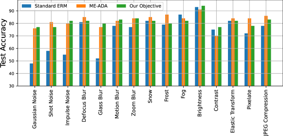
Refer to caption
Figure 6: Robustness to natural shifts in distribution: Plots comparing the performance of standard ERM training and ME-ADA against our method (RCAD) trained on CIFAR-10 benchmark and tested on various distribution shifts in the corrupted CIFAR-10-C benchmark.

C.2 Robustness to natural distribution shifts

Our final set of experiments probe robustness to more systematic distribution shifts using the corrupted CIFAR-10-C dataset [20]. These shifts go beyond the small perturbations introduced by adversarial examples, and are a more faithful reflection of the sorts of perturbations a machine learning model might face “in the wild”.

We compare RCAD to standard ERM and ME-ADA on this benchmark; when all methods are trained on the uncorrupted CIFAR-10 training dataset, but evaluated on different types of corruptions. We report results in Figure 6. Both RCAD and ME-ADA consistently outperform ERM. On certain corruptions (e.g., Gaussian noise, glass blur), RCAD and ME-ADA achieve test accuracies that are around +25%percent25+25\% larger than the ERM baseline. We do not notice any systematic difference in the results of RCAD versus ME-ADA, but note that ME-ADA requires 2×2\times more compute than RCAD because its adversarial examples require multiple gradient steps to compute.

While the main aim of our experiments has been to show that RCAD achieves higher test accuracy, its good performance on robustness benchmarks suggests that it may be a simpler yet appealing choice for practitioners.

Appendix D Analyzing RCAD vs. ERM in a Non-linear Toy Classification Setup

In Section 5 we analyse the solution returned by RCAD and compare it to the ERM solution in a simplified binary classification setting where the hypothesis class consists of linear predictors. We find that the high dimensional linear decision boundary learnt by ERM depends on the noisy dimensions that are spuriously correlated with the label on the training data 𝒟^^𝒟\hat{\mathcal{D}}. On the other hand, our method RCAD corrects this decision boundary by unlearning spurious features. The self-generated examples by RCAD exemplify the spurious correlations, and maximizing entropy on these examples helps the model to drive any learnt components along the noisy dimensions to lower values. In this section, we consider a setup where the true decision boundary is non-linear and the hypothesis class consists of two-layer neural networks with 128128128 hidden units and ReLU activations. In order to induce spurious features in our training data, we stick to high-dimensional inputs.

Typically, in classification problems the true generalizable features span a lower dimensional space (compared to the ambient dimension) [1]. Ideally, we would like to learn classifiers that depend only on these few generalizable features, and remain independent of all the other noisy features. However, training neural networks with the cross-entropy loss and stochastic gradient descent (SGD) often leads to overfitting on training data since the trained model ends up fitting on noisy features with high probability [43, 19]. To simulate this phenomenon, we use a dlimit-from𝑑d-dimensional toy classification problem where the true features are given by the first two-dimensions only, while the rest of the d2𝑑2d-2 dimensions are pure noise.

Refer to caption
(a) ERM
Refer to caption
(b) RCAD (100 epochs)
Refer to caption
(c) RCAD (200 epochs)
Refer to caption
(d) RCAD (300 epochs)
Figure 7: RCAD objective learns decision boundary using only generalizable features: We simulate a high-dimensional non-linear classification problem by projecting a simple 2-d dataset into a 625-dimensional space. (a) Standard ERM training overfits to this dataset, achieving perfect training accuracy by picking up on spurious features. Plotting a 2D projection of the decision boundary along the true features, we see that it poorly separates the data along the generalizable (true) features. (b, c, d) Visualizing our method (RCAD) at different snapshots throughout training, we see that it converges to the true decision boundary using only the generalizable features, thereby achieving a higher test accuracy.

A dataset 𝒟^^𝒟\hat{\mathcal{D}} of 20,000 training examples is generated by first sampling a two-dimensional vector 𝐱~~𝐱\tilde{{\mathbf{x}}} with equal probability from one of two classes supported over two different well separated moon shaped regions (see Figure 7). Here, 𝐱~~𝐱\tilde{{\mathbf{x}}} is a two dimensional vector with label y{0,1}y01{\textnormal{y}}\in\{0,1\}. In our setting, the input dimension d=625𝑑625d=625. Now, in order to construct the final dlimit-from𝑑d-dimensional input 𝐱𝐱{\mathbf{x}} for the classifier using this two dimensional sample 𝐱~~𝐱\tilde{{\mathbf{x}}}, we first append to each sample a vector of (d2=623𝑑2623d-2=623) zeros, and then add add Gaussian noise ϵ𝒩(0,σ2𝑰d)similar-toitalic-ϵ𝒩0superscript𝜎2subscript𝑰𝑑{\mathbf{\epsilon}}\sim\mathcal{N}(0,\sigma^{2}\bm{I}_{d}) where σ=0.1𝜎0.1\sigma=0.1. Note that the noise is added to all dimensions, including the dimensions of the true feature but our results would not change if we choose to only add noise to the last d2𝑑2d-2 dimensions, which would only make the problem easier.

𝐱(𝐱~,0,,0d-2=623 zeros)+ϵ,ϵ𝒩(𝟎,σ𝟐𝐈𝐝)formulae-sequence𝐱~𝐱subscript00d-2=623 zerositalic-ϵsimilar-toitalic-ϵ𝒩0superscript𝜎2subscript𝐈𝐝\displaystyle{\mathbf{x}}\triangleq(\tilde{{\mathbf{x}}},\underbrace{0,\cdots,0}_{\text{d-2=623 zeros}})+{\mathbf{\epsilon}},\qquad{\mathbf{\epsilon}}\sim{\mathcal{N}}(\bf{0},\sigma^{2}\bf{I}_{d})
(d,σ)𝑑𝜎(d,\sigma) ERM Adv. Training (FGSM) ME-ADA RCAD
(625,0.10)6250.10(625,0.10) 80.4%percent80.480.4\% 78.8%percent78.878.8\% 90.9%percent90.990.9\% 94.9%percent94.9\mathbf{94.9\%}
(625,0.75)6250.75(625,0.75) 77.8%percent77.877.8\% 77.9%percent77.977.9\% 84.4%percent84.484.4\% 89.6%percent89.6\mathbf{89.6\%}
(1000,0.10)10000.10(1000,0.10) 74.3%percent74.374.3\% 72.0%percent72.072.0\% 83.5%percent83.583.5\% 87.1%percent87.1\mathbf{87.1\%}
Table 7: In the toy non-linear classification problem, RCAD is found to be more robust to spurious correlations in the training data. We show the test performance of RCAD vs. baseline methods ERM, adversarial training (FGSM) and ME-ADA as we vary two parameters: d𝑑d which is the dimension of the input, and σ𝜎\sigma which is the standard deviation of the noise added to every dimension.

We will measure the in-distribution performance of a classifier, trained on 𝒟^^𝒟\hat{\mathcal{D}} and evaluated on fresh examples from the distribution defined above. In our toy setup, the first two dimensions of the data perfectly explain the class label; we call these dimensions the generalizable (true) features. We are interested in learning non-linear classifiers (two-layer neural nets) that successfully identify these generalizable features, while ignoring the remaining dimensions.

Models trained with the standard cross-entropy loss on a fixed dataset 𝒟^^𝒟\hat{\mathcal{D}} are liable to overfit [67]. A model can best reduce the (empirical) cross-entropy loss by learning features that span all dimensions, including the spurious feature dimensions. Precisely, the model can continue to reduce the cross-entropy loss on some example 𝐱(i)superscript𝐱𝑖{\mathbf{x}}^{(i)} by further aligning some of the weights of its hidden units along the direction of the corresponding noise ϵ(i)superscriptitalic-ϵ𝑖{\mathbf{\epsilon}}^{(i)}, that is part of input 𝐱(i)superscript𝐱𝑖{\mathbf{x}}^{(i)}.

We start by training a two-layer net on 𝒟^^𝒟\hat{\mathcal{D}}. We train it for 300 epochs of SGD using the standard empirical cross entropy loss. This model achieves perfect training accuracy (100%percent100100\%), but performs poorly on the validation set (80.4%percent80.480.4\%). To visualize the learned model, we project the decision boundary on the first two coordinates, the only ones that are truly correlated with the label on population data. The decision boundary for this model, shown in Figure 7(a), is quite different from the true decision boundary. Rather than identifying the true generalizable features, this model has overfit to the noisy dimensions, which are perpendicular to the span of the true features. Training this model for more epochs leads to additional overfitting, further decreasing the test accuracy.

Next we train with our objective RCAD using the same training dataset. In addition to minimizing the standard empirical cross entropy loss, our method also maximizes the predictive entropy of the model on self-generated perturbations that lie along the adversarial directions. Intuitively, we expect that these new examples will be along the directions of the spurious features, exacerbating them. This is because adversarial directions have been shown to comprise of spurious features [22]. Thus, in training the model to be less confident on these examples, we signal the model to unlearn these spurious features. Applying RCAD to this dataset, we achieve a much larger test accuracy of 94.9%percent94.994.9\%. When we visualize the decision boundary (along span of the true features) in Figure 7(d), we observe that it correctly separates the data. While SGD is implicitly biased towards learning simple (e.g., linear) decision boundaries [27], our results show that RCAD partially counters this bias, forcing the model to learn a non-linear decision boundary along the true features and ignoring the noisy dimensions. Additionally we also train adversarial baselines in this setup and compare the test accuracies with RCAD in Table 7. We find that RCAD is less vulnerable to spurious correlations compared to other methods even when we increase the dimensionality of the input or the noise level in the data generating process, both of which would make models more prone to overfitting. This is confirmed by the significant drop in the test performance of the ERM baseline.