Beta Generalized Normal Distribution with an Application for SAR Image Processing

We introduce the beta generalized normal distribution which is obtained by compounding the beta and generalized normal [Nadarajah, S., A generalized normal distribution, Journal of Applied Statistics. 32, 685–694, 2005] distributions. The new model includes as sub-models the beta normal, beta Laplace, normal, and Laplace distributions. The shape of the new distribution is quite flexible, specially the skewness and the tail weights, due to two additional parameters. We obtain general expansions for the moments. The estimation of the parameters is investigated by maximum likelihood. We also proposed a random number generator for the new distribution. Actual synthetic aperture radar were analyzed and modeled after the new distribution. Results could outperform the $\mathcal{G}^{0}$, $\mathcal{K}$, and $\Gamma$ distributions in several scenarios.

Keywords
Beta normal distribution; generalized normal distribution; hazard function; maximum likelihood estimation; moment; SAR imagery

1 Introduction

Sonar, laser, ultrasound B-scanners, and synthetic aperture radar (SAR) are sensing devices which employ coherent illumination for imaging purposes [26]. Due to its capability of operating in any weather condition and providing high spatial image resolution, these microwave active sensors have been considered as powerful remote sensing techniques [27]. In general terms, the operation of these systems consists of the emission of orthogonally polarized pulses transmitted towards a target and the recording of the returned echo signal.

Due to its acquisition process by means of coherent illuminations, SAR images are strongly contaminated by a particular signal-dependent granular noise called speckle [22]. Thus, adequate statistical modeling for this type of imagery is constantly sought [8]. Several distributions have been proposed in the literature for modeling intensity SAR data. According to Frery et al. [12], the $\mathcal{G}^{0}$, $\mathcal{K}$, and $\Gamma$ distributions are the most prominent models for SAR data.

Indeed, a SAR image can be understood as a set of regions described by different probability distributions. Some researchers have devoted considerable attention to study the beta distribution as a model for SAR images. For instance, in [10] the beta distribution was suggested as an important element for modeling SAR images with multi-modal histogram [6].

Eugene et al. [11] introduced a class of distributions generated from the logit of the beta random variable. For a given baseline cumulative distribution function (cdf) $G(x)$, the associated beta generalized distribution $F(x)$ is defined by

$$F(x)=I_{G(x)}(\alpha,\beta)=\frac{1}{\mathrm{B}(\alpha,\beta)}\int_{0}^{G(x)}t^{\alpha-1}(1-t)^{\beta-1}\mathrm{d}t.$$ (1)

Here, $\alpha>0$ and $\beta>0$ are two additional parameters which aim to introduce skewness and to vary tail weights, $I_{y}(\alpha,\beta)=\mathrm{B}_{y}(\alpha,\beta)/\mathrm{B}(\alpha,\beta)$ is the incomplete beta function ratio, $\mathrm{B}_{y}(\alpha,\beta)=\int_{0}^{y}w^{\alpha-1}(1-w)^{\beta-1}\mathrm{d}w$ is the incomplete beta function, $\mathrm{B}(\alpha,\beta)=\Gamma(\alpha)\Gamma(\beta)/\Gamma(\alpha+\beta)$ is the beta function and $\Gamma(\cdot)$ is the gamma function. This class of beta generalized distributions has been receiving considerable attention after the work of Eugene et al. [11].

The beta distribution is a basic exemplar of (1) by taking $G(x)=x$. Although it has only two parameters, the beta density accommodates a very wide variety of shapes including the standard uniform distribution for $\alpha=\beta=1$. The beta density is symmetric, unimodal, and bathtub shaped for $\alpha=\beta$, $\alpha,\,\beta>1$ and $\alpha,\,\beta<1$, respectively. It has positive skew when $\alpha<\beta$ and negative skew when $\alpha>\beta$.

Some special beta generalized distributions were developed in recent years. To cite a few, we identify the beta normal distribution [11], the beta Gumbel distribution [20], the beta Frechet distribution [19], the beta exponential distribution [21], the beta Weibull distribution [16], the beta Pareto distribution [2], the beta generalized exponential distribution [3], and the beta generalized half-normal distribution [23].

The first goal of this note is to develop an extension of the generalized normal (GN) distribution defined from (1): the beta generalized normal (BGN) distribution. It may be mentioned that although several skewed distribution functions exist on the positive real axis, but not many skewed distributions are available on the whole real line, which are easy to use for data analysis purpose. The main role of the extra parameters $\alpha$ and $\beta$ is that the BGN distribution can be used to model skewed real data, a feature which is very common in practice. The BGN distribution with five parameters to control location, dispersion, modality and skewness has great flexibility.

As a second goal, we emphasize the BGN distribution ability for modeling bimodal phenomena, which naturally occurs in the context of image processing of SAR imagery [10]. Thus, the BGN distribution is a candidate to SAR data modeling. We sought a data analysis using simulated and actual SAR imagery. Also, we compare the BGN model with several existing models for SAR, such as the gamma distribution [5], the $\mathcal{K}$ distribution [4], and the $\mathcal{G}^{0}$ distribution [12]. The gamma distribution is regarded as standard model for the herein considered types of SAR data [5]. For such, actual data is analyzed and fitted according to all models above, where the original and corrected Akaike information and Bayesian information criteria are employed as the goodness-of-fit measures [13].

The rest of the paper is organized as follows. In Section 2, we define the BGN distribution, derive its density, and discuss particular cases. General expansions for the moments are derived in Section 3. Maximum likelihood estimation is investigated in Section 4. In Section 5, we propose a random number generator for the new distribution. Section 6 details the SAR image analysis based on actual data. Section 7 gives some concluding remarks.

2 The BGN Distribution

The GN distribution with location parameter $\mu$, dispersion parameter $\sigma$ and shape parameter $s$ has probability density function (pdf) given by [17]

$$g(x)=\frac{s}{2\sigma\,\Gamma(1/s)}\exp\left\{-\left|\frac{x-\mu}{\sigma}\right|^{s}\right\},\quad x\in\mathbb{R},$$

where $\mu$ is a real number, and $\sigma$ and $s$ are positive real numbers. For the special case $s=1$, the above density function reduces to the Laplace distribution with location parameter $\mu$ and scale parameter $\sigma$. Similarly, for $s=2$, the normal distribution is obtained with mean $\mu$ and variance $\sigma^{2}/2$. The main feature of the GN model is that new parameter $s$ can introduce some skewness and kurtosis.

The GN cumulative function can be expressed as follows [17, Eq. 5-6]

$$G(x)=\begin{cases}\frac{\Gamma(1/s,(\frac{\mu-x}{\sigma})^{s})}{2\Gamma(1/s)},&x\leq\mu,\\ 1-\frac{\Gamma(1/s,(\frac{x-\mu}{\sigma})^{s})}{2\Gamma(1/s)},&x>\mu,\end{cases}$$ (2)

where $\Gamma(s,x)=\int_{x}^{\infty}t^{s-1}\exp(-t)\mathrm{d}t$ is the complementary incomplete gamma function.

The density function of the standardized random variable $Z=(X-\mu)/\sigma$ is

$$\phi_{s}(z)=\frac{s}{2\Gamma(1/s)}\exp(-|z|^{s}),\quad z\in\mathbb{R}.$$

Thus, $g(x)=\sigma^{-1}\,\phi_{s}(\frac{x-\mu}{\sigma})$. From (2), the cdf of the standardized GN distribution reduces to

$$\Phi_{s}(z)=\begin{cases}\frac{\Gamma(1/s,(-z)^{s})}{2\Gamma(1/s)},&z\leq 0,\\ 1-\frac{\Gamma(1/s,z^{s})}{2\Gamma(1/s)},&z>0.\end{cases}$$ (3)

Based on equation (1), we propose a natural generalization of the GN distribution and provide a comprehensive treatment of its mathematical properties. The cdf of the BGN distribution is

$$F(x)=\frac{1}{\mathrm{B}(\alpha,\beta)}\int_{0}^{\Phi_{s}(\frac{x-\mu}{\sigma})}t^{\alpha-1}\,(1-t)^{\beta-1}\,\mathrm{d}t=I_{\Phi_{s}(\frac{x-\mu}{\sigma})}(\alpha,\beta).$$

Consequently, its density function reduces to

$$f(x)=\frac{1}{\sigma\mathrm{B}(\alpha,\beta)}\,\left[\Phi_{s}\left(\frac{x-\mu}{\sigma}\right)\right]^{\alpha-1}\left[1-\Phi_{s}\left(\frac{x-\mu}{\sigma}\right)\right]^{\beta-1}\phi_{s}\left(\frac{x-\mu}{\sigma}\right).$$ (4)

Here, the parameters $\alpha$ and $\beta$ control skewness through the relative tail weights. They provide greater flexibility in the form of the distribution and consequently in modeling observed real data. A random variable $X$ with density function (4) is denoted by BGN$(\alpha,\beta,\mu,\sigma,s)$. Clearly, the beta normal and beta Laplace distributions are special models of (4) corresponding to $s=1$ and $s=2$, respectively. The GN distribution is a special sub-model for $\alpha=\beta=1$. The normal distribution arises for $\alpha=\beta=1$ and $s=2$, whereas the Laplace distribution corresponds to $\alpha=\beta=s=1$. Location and scale parameters are redundant in (4), since if $X\sim$BGN$(\alpha,\beta,0,1,s)$ then $Y=\sigma\,X+\mu\sim$BGN$(\alpha,\beta,\mu,\sigma,s)$.

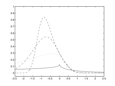
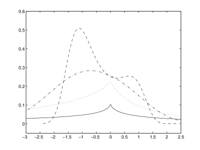
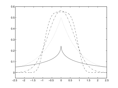
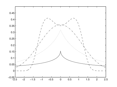
Figure 1 displays the BGN density function (4) for selected parameter values. As parameters vary, several useful features, such as bi-modality and pronounced skewness, can be obtained. These facts illustrate the flexibility of the BGN distribution to analyze real data.

(a) $\alpha=\beta=1$

(b) $\alpha=\beta=0.5$

(c) $\alpha=0.5,\beta=2$

(d) $\alpha=0.25,\beta=0.5$

Figure 1: Plots of the BGN density function for some parameter values: $\mu=0$, $\sigma=1$, and $s\in\{1/2,1,2,4\}$ (solid, dotted, dash-dotted, and dashed, respectively).

Note that the limiting behavior of the GN density with respect to $s$ is given by

$$\lim_{s\to\infty}\phi_{s}(z)=\lim_{s\to\infty}\frac{s}{2\Gamma(1/s)}\exp(-|z|^{s})=\begin{cases}\frac{1}{2},&|z|<1,\\ 0,&\text{otherwise.}\end{cases}$$

Consequently, the dominate convergence theorem leads to

$$\lim_{s\to\infty}\Phi_{s}(z)=\begin{cases}0,&z<-1,\\ \frac{1}{2}(z+1),&|z|<1,\\ 1,&z>1.\end{cases}$$

Making appropriate substitutions, we conclude that the limiting distribution $\lim_{s\to\infty}f(x)$ is related to the usual beta distribution

$$\lim_{s\to\infty}f(x) =\frac{1}{2\sigma}f_{\text{Beta}}\left(\frac{1}{2}\left(\frac{x-\mu}{\sigma}+1\right)\right),\quad x\in[\mu-\sigma,\mu+\sigma],$$ (5)

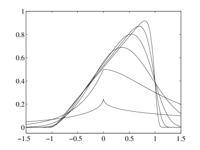
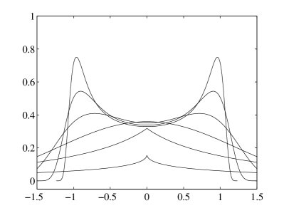
where $f_{\text{Beta}}(x)=\frac{1}{\mathrm{B}(\alpha,\beta)}x^{\alpha-1}\,(1-x)^{\beta-1}$ is the beta density defined over $x\in[0,1]$. Figure 2 illustrates this behavior. As $s$ increases, plots in Figures 2(a) and 2(b) tend to the U-shaped and triangular density functions, respectively, which are special models of the beta distribution. Figure 3 depicts a diagram with the relations among the discussed models.

(a) $\alpha=\beta=0.5$

(b) $\alpha=2,\beta=1$

Figure 2: Limiting behavior of the BGN density function for increasing values of $s\in\{1/2,1,2,4,8,16\}$, $\mu=0$, and $\sigma=1$: (a) U-shaped beta density and (b) triangular density.

Figure 3: Diagram relating the current models.

3 Moments

Let $X$ be a random variable having the BGN$(\alpha,\beta,\mu,\sigma,s)$ distribution. The $n$th moment of $X$ becomes

$$\mathrm{E}(X^{n})=\frac{1}{\mathrm{B}(\alpha,\beta)}\frac{1}{\sigma}\int_{-\infty}^{\infty}x^{n}\left[\Phi_{s}\left(\frac{x-\mu}{\sigma}\right)\right]^{\alpha-1}\left[1-\Phi_{s}\left(\frac{x-\mu}{\sigma}\right)\right]^{\beta-1}\phi_{s}\left(\frac{x-\mu}{\sigma}\right)\mathrm{d}x.$$

Proposition 1

The $n$th moment of $X$ can be expressed as

$$\begin{split}\mathrm{E}(X^{n})=&\frac{\mu^{n}}{\mathrm{B}(\alpha,\beta)}\sum_{j=0}^{\infty}(-1)^{j}\binom{\beta-1}{j}\sum_{i=0}^{n}\binom{n}{i}\left(\frac{\sigma}{\mu}\right)^{i}\\ &\times\sum_{k=0}^{\infty}\left[v_{k}(j+\alpha-1)+(-1)^{i+k}\binom{j+\alpha-1}{k}\right]J_{i,k}^{(s)},\end{split}$$ (6)

where

$$v_{k}(\alpha)=\sum_{m=k}^{\infty}(-1)^{k+m}\,\binom{\alpha}{m}\,\binom{m}{k}$$

and

$$J_{i,k}^{(s)}=\int_{0}^{\infty}z^{i}\,\phi_{s}(z)\,\Phi_{s}(z)^{k}\mathrm{d}z.$$

The above proposition is proved in Appendix A. It is also clear that the evaluation of the $n$th moment is related to the computation of $J_{i,k}^{(s)}$. Appendix B provides an expansion derivation for $J_{i,k}^{(s)}$, as shown in (10).

4 Maximum Likelihood Estimation

Consider a random variable having the BGN distribution and let $\mathbf{\theta}=(s,\mu,\sigma,\alpha,\beta)^{T}$ be its parameter vector. The log-likelihood for a particular observation is

$$\ell(\mathbf{\theta})= -\log\mathrm{B}(\alpha,\beta)-\log\sigma+(\alpha-1)\log\Phi_{s}\left(\frac{x-\mu}{\sigma}\right)$$

$$+(\beta-1)\log\left[1-\Phi_{s}\left(\frac{x-\mu}{\sigma}\right)\right]+\log\phi_{s}\left(\frac{x-\mu}{\sigma}\right).$$

To evaluate the unit score vector $\left(\frac{\mathrm{d}}{\mathrm{d}s}\ell,\frac{\mathrm{d}}{\mathrm{d}\mu}\ell,\frac{\mathrm{d}}{\mathrm{d}\sigma}\ell,\frac{\mathrm{d}}{\mathrm{d}\alpha}\ell,\frac{\mathrm{d}}{\mathrm{d}\beta}\ell\right)^{T}$, simple algebra yields

$$\frac{\mathrm{d}}{\mathrm{d}s}\ell\left[\frac{\alpha-1}{\Phi_{s}\left(\frac{x-\mu}{\sigma}\right)}-\frac{\beta-1}{1-\Phi_{s}\left(\frac{x-\mu}{\sigma}\right)}\right]\frac{\mathrm{d}}{\mathrm{d}s}\Phi_{s}\left(\frac{x-\mu}{\sigma}\right)+\frac{\mathrm{d}}{\mathrm{d}s}\log\phi_{s}\left(\frac{x-\mu}{\sigma}\right).$$

From the definition of $\Phi_{s}$ given in (3), it is clear that $\frac{\mathrm{d}}{\mathrm{d}s}\Phi_{s}\left(\frac{x-\mu}{\sigma}\right)$ depends on the derivatives of the gamma and the incomplete gamma functions. Then, these particular derivatives deserve close examination as follows. For $x>0$, the following derivative holds [1, 14]:

$$\frac{\mathrm{d}}{\mathrm{d}s}\Gamma(1/s,x^{s}) =-\frac{1}{s^{2}}\Big{[}\log(x^{s})\Gamma(1/s,x^{s})+x^{s}T(3,1/s,x^{s})\Big{]}-x\exp(-x^{s})\log(x)$$

$$\triangleq\tilde{\psi}(s,x),$$

where the quantity $\tilde{\psi}(s,x)$ is an auxiliary function for the sake of convenience of manipulation and $T(3,\cdot,\cdot)$ is a particular case of the Meijer $G$-function given by [14, p. 156]:

$$T(3,a,x)= G_{2}^{3}\,{}_{3}^{0}\left(x\left|\begin{matrix}0,0\\ -1,a-1,-1\end{matrix}\right.\right)$$

$$= \frac{x^{a-1}{}_{2}\mathrm{F}_{2}\left(a,a;1+a,1+a;-x\right)}{a^{2}}-\frac{\Gamma(a)\log(x)}{x}+\frac{\Gamma(a)\psi(a)}{x},$$

where $\psi(\cdot)$ is the digamma function. Consequently, after some manipulations, we obtain

$$\frac{\mathrm{d}}{\mathrm{d}s}\Phi_{s}\left(\frac{x-\mu}{\sigma}\right) =\frac{1}{2\Gamma(1/s)}\begin{cases}s^{2}\tilde{\psi}\left(s,(\frac{\mu-x}{\sigma})^{s}\right)+\psi(1/s)\Gamma(1/s,(\frac{\mu-x}{\sigma})^{s}),&x\leq\mu,\\ -[s^{2}\tilde{\psi}\left(s,(\frac{x-\mu}{\sigma})^{s}\right)+\psi(1/s)\Gamma(1/s,(\frac{x-\mu}{\sigma})^{s})],&x>\mu.\end{cases}$$

Another required quantity is the following:

$$\log\phi_{s}\left(\frac{x-\mu}{\sigma}\right) =\log\left[\frac{s}{2\Gamma(1/s)}\exp\left(-\left|\frac{x-\mu}{\sigma}\right|^{s}\right)\right]$$

$$=\log s-\log(2\Gamma(1/s))-\left|\frac{x-\mu}{\sigma}\right|^{s}.$$

Therefore, we have

$$\frac{\mathrm{d}}{\mathrm{d}s}\log\phi_{s}\left(\frac{x-\mu}{\sigma}\right) =\frac{1}{s}+\frac{\psi(1/s)}{s^{2}}-\left|\frac{x-\mu}{\sigma}\right|^{s}\log\left(\left|\frac{x-\mu}{\sigma}\right|\right).$$

Now, we examine the derivatives of $\ell$ with respect to $\mu$ and $\sigma$. They are given by

$$\frac{\mathrm{d}}{\mathrm{d}\mu}\ell= -\frac{\alpha-1}{\sigma}\frac{\phi_{s}\left(\frac{x-\mu}{\sigma}\right)}{\Phi_{s}\left(\frac{x-\mu}{\sigma}\right)}+\frac{\beta-1}{\sigma}\frac{\phi_{s}\left(\frac{x-\mu}{\sigma}\right)}{1-\Phi_{s}\left(\frac{x-\mu}{\sigma}\right)}+\frac{s}{\sigma}\left|\frac{x-\mu}{\sigma}\right|^{s-1}\mathrm{sign}(x-\mu)$$

and

$$\frac{\mathrm{d}}{\mathrm{d}\sigma}\ell= -\frac{1}{\sigma}-\frac{\alpha-1}{\sigma^{2}}(x-\mu)\frac{\phi_{s}\left(\frac{x-\mu}{\sigma}\right)}{\Phi_{s}\left(\frac{x-\mu}{\sigma}\right)}+\frac{\beta-1}{\sigma^{2}}(x-\mu)\frac{\phi_{s}\left(\frac{x-\mu}{\sigma}\right)}{1-\Phi_{s}\left(\frac{x-\mu}{\sigma}\right)}-\frac{s}{\sigma}\left|\frac{x-\mu}{\sigma}\right|^{s},$$

respectively, where we use the fact that $|x|=x\,\mathrm{sign}(x)$.

In order to calculate the derivative with respect to $\alpha$, note that:

$$\frac{\mathrm{d}}{\mathrm{d}\alpha}\log\mathrm{B}(\alpha,\beta) =\psi(\alpha)-\psi(\alpha+\beta).$$

Therefore, it follows immediately that

$$\frac{\mathrm{d}}{\mathrm{d}\alpha}\ell= \psi(\alpha+\beta)-\psi(\alpha)+\log\Phi_{s}\left(\frac{x-\mu}{\sigma}\right)$$

and

$$\frac{\mathrm{d}}{\mathrm{d}\beta}\ell= \psi(\alpha+\beta)-\psi(\beta)+\log\left[1-\Phi_{s}\left(\frac{x-\mu}{\sigma}\right)\right].$$

5 BGN Random Number Generator

In this section, a random number generator (RNG) for the BGN distribution is introduced. This RNG allows a Monte Carlo study to determine the influence of the BGN shape parameters $\alpha$, $\beta$, and $s$.

We consider the inverse transform algorithm for generating continuous random variables [24, p. 67]. Indeed, a BGN random variable $X\sim\text{BGN}(\alpha,\beta,\mu,\sigma,s)$ can be related to a beta distributed random variable $U\sim\operatorname{B}(\alpha,\beta)$ according to $X=G^{-1}(U)$, where $G$ is given in (2). Notice that

$$G(x)=\begin{cases}\frac{1}{2}\left\{1-F_{\Gamma}\left[\left(-\frac{x-\mu}{\sigma}\right)^{s}\right]\right\},&x\leq\mu,\\ \frac{1}{2}\left\{1+F_{\Gamma}\left[\left(\frac{x-\mu}{\sigma}\right)^{s}\right]\right\},&x>\mu,\end{cases}$$

where $F_{\Gamma}(\cdot)$ is the cdf of the gamma distribution with shape and scape parameters given by $1/s$ and 1, respectively.

Let $x$ and $u$ be realizations of $X$ and $U$, respectively. For $x\leq\mu$, we obtain the inverse transformation according to the following manipulation

$$\frac{1}{2}\left\{1-F_{\Gamma}\left[\left(-\frac{x-\mu}{\sigma}\right)^{s}\right]\right\}=u.$$

Therefore,

$$x=\mu-\sigma\left[F^{-1}_{\Gamma}(1-2u)\right]^{1/s},$$

where $F^{-1}_{\Gamma}(\cdot)$ is the quantile function of the gamma distribution with parameters $1/s$ and 1. Since $0\leq F_{\Gamma}\left[\left(-\frac{x-\mu}{\sigma}\right)^{s}\right]\leq 1$, we have $0\leq u\leq 1/2$.

Analogously, for $x>\mu$, we obtain

$$x=\mu+\sigma\left[F^{-1}_{\Gamma}(2u-1)\right]^{1/s},\quad 1/2<u\leq 1.$$

Therefore, the RNG for $X$ can be algorithmically described as follows:

1:Generate $U\sim\text{beta}(\alpha,\beta)$

2:if $U\in[0,1/2]$ then

3:     $X=\mu-\sigma\left[F^{-1}_{\Gamma}(1-2u)\right]^{1/s}$

4:else

5:     $X=\mu+\sigma\left[F^{-1}_{\Gamma}(2u-1)\right]^{1/s}$

6:return $X$.

Figure 4 displays four cases where theoretical curves are compared with randomly generated points for $\alpha=0.1$, $\beta=0.3$, $\mu=0$, $\sigma=1$, and $s\in\{2,4,6,12\}$.

\psfrag{BGN1}[c][c][1.0]{\;\;\;\;\;\scriptsize{Generated values}}\psfrag{BGN2}[c][c][1.0]{\;\;\;\;\;\scriptsize{Generated values}}\psfrag{BGN3}[c][c][1.0]{\;\;\;\;\;\scriptsize{Generated values}}\psfrag{BGN4}[c][c][1.0]{\;\;\;\;\;\scriptsize{Generated values}}\psfrag{Density}[c][c][1.0]{\;\;\;\;\;\scriptsize{Density}}\includegraphics[width=208.13574pt]{BGNsimulated1}

(a) BGN($0.1,0.3,0,1,2$)

\psfrag{BGN1}[c][c][1.0]{\;\;\;\;\;\scriptsize{Generated values}}\psfrag{BGN2}[c][c][1.0]{\;\;\;\;\;\scriptsize{Generated values}}\psfrag{BGN3}[c][c][1.0]{\;\;\;\;\;\scriptsize{Generated values}}\psfrag{BGN4}[c][c][1.0]{\;\;\;\;\;\scriptsize{Generated values}}\psfrag{Density}[c][c][1.0]{\;\;\;\;\;\scriptsize{Density}}\includegraphics[width=208.13574pt]{BGNsimulated2}

(b) BGN($0.1,0.3,0,1,4$)

\psfrag{BGN1}[c][c][1.0]{\;\;\;\;\;\scriptsize{Generated values}}\psfrag{BGN2}[c][c][1.0]{\;\;\;\;\;\scriptsize{Generated values}}\psfrag{BGN3}[c][c][1.0]{\;\;\;\;\;\scriptsize{Generated values}}\psfrag{BGN4}[c][c][1.0]{\;\;\;\;\;\scriptsize{Generated values}}\psfrag{Density}[c][c][1.0]{\;\;\;\;\;\scriptsize{Density}}\includegraphics[width=208.13574pt]{BGNsimulated3}

(c) BGN($0.1,0.3,0,1,6$)

\psfrag{BGN1}[c][c][1.0]{\;\;\;\;\;\scriptsize{Generated values}}\psfrag{BGN2}[c][c][1.0]{\;\;\;\;\;\scriptsize{Generated values}}\psfrag{BGN3}[c][c][1.0]{\;\;\;\;\;\scriptsize{Generated values}}\psfrag{BGN4}[c][c][1.0]{\;\;\;\;\;\scriptsize{Generated values}}\psfrag{Density}[c][c][1.0]{\;\;\;\;\;\scriptsize{Density}}\includegraphics[width=208.13574pt]{BGNsimulated4}

(d) BGN($0.1,0.3,0,1,12$)

Figure 4: BGN random number generation.

6 SAR Image Processing

In this section, we assess the proposed statistical modeling by means of simulated and actual data analysis. First, we employ the proposed BGN RNG to generate synthetic data to be submitted to ML estimation. We show evidence of the effectiveness of the derived methods. Subsequently, we employ ML estimation to actual SAR data aiming their statistical modeling.

6.1 Influence Study Based on Shape Parameters

To assess the effect of the shape parameters, we performed a Monte Carlo simulation with $M=10^{3}$ replications.

For each replication the following steps were considered:

1. Simulated BGN distributed images of $7\times 7$, $11\times 11$, and $20\times 20$ pixels were obtained by means of the BGN RNG furnishing sample sizes of $N\in\{49,121,400\}$.

2. Three scenarios were considered: (a) $\alpha=1$, $\beta=1$, and $s\in\{1,1.5,2,1.5,3,3.5,4,4.5,5\}$; (b) $\alpha=1$, $\beta\in\{1,1.5,2,1.5,3,3.5,4,4.5,5\}$, and $s=1$; and (c) $\alpha\in\{1,1.5,2,1.5,3,3.5,4,4.5,5\}$, $\beta=1$, and $s=1$. In all cases, $\mu=0$, and $\sigma=1$;

3. Generated data was submitted to ML estimation to obtain estimate parameters and an estimated BGN pdf $\hat{f}(\cdot)$;

4. Squared errors between the exact and estimated pdfs were computed.

This procedure was repeated $M$ times, which furnished the mean squared error (MSE). Figure 5 displays the relationship between shape parameters and the MSE.

As expected from the ML estimation asymptotic properties, in general terms, the influence on the MSE diminishes when the sample size increases.

\psfrag{g1}[c][c][1.0]{\;\;\;\;\;\scriptsize{$\hskip 24.11108pt\beta\colon\alpha=s=1$}}\psfrag{g2}[c][c][1.0]{\;\;\;\;\;\scriptsize{$\hskip 23.2069pt\alpha\colon\beta=s=1$}}\psfrag{g3}[c][c][1.0]{\;\;\;\;\;\scriptsize{$\hskip 25.01526pts\colon\alpha=\beta=1$}}\psfrag{Influence}[c][c][1.0]{\;\;\;\;\;\scriptsize{MSE}}\psfrag{ABA}[c][c][1.0]{\;\;\;\;\;\scriptsize{Parameter values}}\includegraphics[width=208.13574pt]{influencesize1}

(a) $N=49$

\psfrag{g1}[c][c][1.0]{\;\;\;\;\;\scriptsize{$\hskip 24.11108pt\beta\colon\alpha=s=1$}}\psfrag{g2}[c][c][1.0]{\;\;\;\;\;\scriptsize{$\hskip 23.2069pt\alpha\colon\beta=s=1$}}\psfrag{g3}[c][c][1.0]{\;\;\;\;\;\scriptsize{$\hskip 25.01526pts\colon\alpha=\beta=1$}}\psfrag{Influence}[c][c][1.0]{\;\;\;\;\;\scriptsize{MSE}}\psfrag{ABA}[c][c][1.0]{\;\;\;\;\;\scriptsize{Parameter values}}\includegraphics[width=208.13574pt]{influencesize2}

(b) $N=121$

\psfrag{g1}[c][c][1.0]{\;\;\;\;\;\scriptsize{$\hskip 24.11108pt\beta\colon\alpha=s=1$}}\psfrag{g2}[c][c][1.0]{\;\;\;\;\;\scriptsize{$\hskip 23.2069pt\alpha\colon\beta=s=1$}}\psfrag{g3}[c][c][1.0]{\;\;\;\;\;\scriptsize{$\hskip 25.01526pts\colon\alpha=\beta=1$}}\psfrag{Influence}[c][c][1.0]{\;\;\;\;\;\scriptsize{MSE}}\psfrag{ABA}[c][c][1.0]{\;\;\;\;\;\scriptsize{Parameter values}}\includegraphics[width=208.13574pt]{influencesize3}

(c) $N=400$

Figure 5: Mean square error for several pararameter values.

6.2 SAR Image Modeling

In recent years, the interest in understanding such type of imagery in a multidimensional and multilook perspective has increased. In this case, the current data is termed multilook polarimetric SAR (PolSAR). In such situation, backscattered signals are recorded as complex elements for all possible combinations of linear reception and transmission polarizations: HH, HV, and VV (H for horizontal and V for vertical polarization). In particular, the intensity of the echoed signal polarization channels plays an important role, since it depends on the physical properties of the target surface. Figure 6(a) presents an image over the surroundings of Foulum (Denmark) obtained by the SAR system EMISAR [7]. This is a polarimetric SAR image, i.e., their pixels are represented by 3$\times$3 Hermitian positive definite matrices whose diagonal elements are positive real intensities: denominated by HH, HV, and VV.

\psfrag{A1}[c][c][1.0]{\footnotesize{\quad\quad\quad\quad\quad\quad\quad\color[rgb]{1,1,1}{A}1}}\psfrag{A2}[c][c][1.0]{\footnotesize{\quad\color[rgb]{0,0,0}{A}2}}\psfrag{A3}[c][c][1.0]{\footnotesize{\color[rgb]{1,1,1}{A}3}}\psfrag{A}[c][c][1.0]{\;\;\;\;\;\tiny{BGN}}\psfrag{B}[c][c][1.0]{\;\;\;\;\;\;\;\;\;\tiny{GAMMA}}\psfrag{YP}[c][c][1.0]{\tiny{Empirical Density}}\psfrag{YP1}[c][c][1.0]{\tiny{Empirical Density}}\psfrag{XP}[c][c][1.0]{\tiny{Returned Signal Intensity}}\psfrag{XP1}[c][c][1.0]{\tiny{Returned Signal Intensity}}\psfrag{Density}[c][c][1.0]{\;\;\;\;\;\footnotesize{Density}}\psfrag{HH1}[c][c][1.0]{\;\;\;\;\;\footnotesize{Intensity ($\times$ 10${}^{-2}$)}}\psfrag{HH2}[c][c][1.0]{\;\;\;\;\;\footnotesize{Intensity ($\times$ 10${}^{-1}$)}}\psfrag{HH3}[c][c][1.0]{\;\;\;\;\;\footnotesize{Intensity ($\times$ 10${}^{-3}$)}}\psfrag{HV1}[c][c][1.0]{\;\;\;\;\;\footnotesize{Intensity ($\times$ 10${}^{-3}$)}}\psfrag{HV2}[c][c][1.0]{\;\;\;\;\;\footnotesize{Intensity ($\times$ 10${}^{-2}$)}}\psfrag{HV3}[c][c][1.0]{\;\;\;\;\;\footnotesize{Intensity ($\times$ 10${}^{-4}$)}}\psfrag{VV1}[c][c][1.0]{\;\;\;\;\;\footnotesize{Intensity ($\times$ 10${}^{-2}$)}}\psfrag{VV2}[c][c][1.0]{\;\;\;\;\;\footnotesize{Intensity ($\times$ 10${}^{-2}$)}}\psfrag{VV3}[c][c][1.0]{\;\;\;\;\;\footnotesize{Intensity ($\times$ 10${}^{-3}$)}}\psfrag{0}[c][c][1.0]{\tiny{0}}\psfrag{500}[c][c][1.0]{\tiny{500}}\psfrag{1000}[c][c][1.0]{\tiny{1000}}\psfrag{1500}[c][c][1.0]{\tiny{1500}}\psfrag{2000}[c][c][1.0]{\tiny{2000}}\psfrag{4000}[c][c][1.0]{\tiny{4000}}\psfrag{6000}[c][c][1.0]{\tiny{6000}}\psfrag{8000}[c][c][1.0]{\tiny{8000}}\psfrag{2e-04}[c][c][1.0]{\tiny{2}}\psfrag{4e-04}[c][c][1.0]{\tiny{4}}\psfrag{6e-04}[c][c][1.0]{\tiny{6}}\psfrag{8e-04}[c][c][1.0]{\tiny{8}}\psfrag{1e-03}[c][c][1.0]{\tiny{10}}\psfrag{0.0010}[c][c][1.0]{\tiny{1.0}}\psfrag{0.0015}[c][c][1.0]{\tiny{1.5}}\psfrag{0.0020}[c][c][1.0]{\tiny{2.0}}\psfrag{0.0025}[c][c][1.0]{\tiny{2.5}}\psfrag{0.0030}[c][c][1.0]{\tiny{3.0}}\psfrag{0.0035}[c][c][1.0]{\tiny{3.5}}\psfrag{0.000}[c][c][1.0]{\tiny{0}}\psfrag{0.001}[c][c][1.0]{\tiny{1}}\psfrag{0.002}[c][c][1.0]{\tiny{2}}\psfrag{0.003}[c][c][1.0]{\tiny{3}}\psfrag{0.004}[c][c][1.0]{\tiny{4}}\psfrag{0.005}[c][c][1.0]{\tiny{5}}\psfrag{0.010}[c][c][1.0]{\tiny{10}}\psfrag{0.015}[c][c][1.0]{\tiny{15}}\psfrag{0.020}[c][c][1.0]{\tiny{20}}\psfrag{1}[c][c][1.0]{\tiny{1}}\psfrag{2}[c][c][1.0]{\tiny{2}}\psfrag{3}[c][c][1.0]{\tiny{3}}\psfrag{4}[c][c][1.0]{\tiny{4}}\psfrag{5}[c][c][1.0]{\tiny{5}}\psfrag{6}[c][c][1.0]{\tiny{6}}\psfrag{8}[c][c][1.0]{\tiny{8}}\psfrag{10}[c][c][1.0]{\tiny{10}}\psfrag{12}[c][c][1.0]{\tiny{12}}\psfrag{14}[c][c][1.0]{\tiny{14}}\psfrag{15}[c][c][1.0]{\tiny{15}}\psfrag{20}[c][c][1.0]{\tiny{20}}\psfrag{30}[c][c][1.0]{\tiny{30}}\psfrag{100}[c][c][1.0]{\tiny{100}}\psfrag{200}[c][c][1.0]{\tiny{200}}\psfrag{300}[c][c][1.0]{\tiny{300}}\psfrag{400}[c][c][1.0]{\tiny{400}}\psfrag{0.00}[c][c][1.0]{\tiny{0}}\psfrag{0.05}[c][c][1.0]{\tiny{5}}\psfrag{0.10}[c][c][1.0]{\tiny{10}}\psfrag{0.15}[c][c][1.0]{\tiny{15}}\psfrag{0.20}[c][c][1.0]{\tiny{20}}\psfrag{0.25}[c][c][1.0]{\tiny{25}}\psfrag{0.30}[c][c][1.0]{\tiny{30}}\psfrag{0.00}[c][c][1.0]{\tiny{0}}\psfrag{0.05}[c][c][1.0]{\tiny{5}}\psfrag{0.10}[c][c][1.0]{\tiny{10}}\psfrag{0.15}[c][c][1.0]{\tiny{15}}\psfrag{0.20}[c][c][1.0]{\tiny{20}}\psfrag{0.25}[c][c][1.0]{\tiny{25}}\psfrag{0.30}[c][c][1.0]{\tiny{30}}\psfrag{0.0}[c][c][1.0]{\tiny{0}}\psfrag{0.2}[c][c][1.0]{\tiny{2}}\psfrag{0.4}[c][c][1.0]{\tiny{4}}\psfrag{0.6}[c][c][1.0]{\tiny{6}}\psfrag{0.8}[c][c][1.0]{\tiny{8}}\includegraphics[width=173.44534pt]{FolumSAR.editedIII.eps}

(a) Foulum (Denmark)

\psfrag{A1}[c][c][1.0]{\footnotesize{\quad\quad\quad\quad\quad\quad\quad\color[rgb]{1,1,1}{A}1}}\psfrag{A2}[c][c][1.0]{\footnotesize{\quad\color[rgb]{0,0,0}{A}2}}\psfrag{A3}[c][c][1.0]{\footnotesize{\color[rgb]{1,1,1}{A}3}}\psfrag{A}[c][c][1.0]{\;\;\;\;\;\tiny{BGN}}\psfrag{B}[c][c][1.0]{\;\;\;\;\;\;\;\;\;\tiny{GAMMA}}\psfrag{YP}[c][c][1.0]{\tiny{Empirical Density}}\psfrag{YP1}[c][c][1.0]{\tiny{Empirical Density}}\psfrag{XP}[c][c][1.0]{\tiny{Returned Signal Intensity}}\psfrag{XP1}[c][c][1.0]{\tiny{Returned Signal Intensity}}\psfrag{Density}[c][c][1.0]{\;\;\;\;\;\footnotesize{Density}}\psfrag{HH1}[c][c][1.0]{\;\;\;\;\;\footnotesize{Intensity ($\times$ 10${}^{-2}$)}}\psfrag{HH2}[c][c][1.0]{\;\;\;\;\;\footnotesize{Intensity ($\times$ 10${}^{-1}$)}}\psfrag{HH3}[c][c][1.0]{\;\;\;\;\;\footnotesize{Intensity ($\times$ 10${}^{-3}$)}}\psfrag{HV1}[c][c][1.0]{\;\;\;\;\;\footnotesize{Intensity ($\times$ 10${}^{-3}$)}}\psfrag{HV2}[c][c][1.0]{\;\;\;\;\;\footnotesize{Intensity ($\times$ 10${}^{-2}$)}}\psfrag{HV3}[c][c][1.0]{\;\;\;\;\;\footnotesize{Intensity ($\times$ 10${}^{-4}$)}}\psfrag{VV1}[c][c][1.0]{\;\;\;\;\;\footnotesize{Intensity ($\times$ 10${}^{-2}$)}}\psfrag{VV2}[c][c][1.0]{\;\;\;\;\;\footnotesize{Intensity ($\times$ 10${}^{-2}$)}}\psfrag{VV3}[c][c][1.0]{\;\;\;\;\;\footnotesize{Intensity ($\times$ 10${}^{-3}$)}}\psfrag{0}[c][c][1.0]{\tiny{0}}\psfrag{500}[c][c][1.0]{\tiny{500}}\psfrag{1000}[c][c][1.0]{\tiny{1000}}\psfrag{1500}[c][c][1.0]{\tiny{1500}}\psfrag{2000}[c][c][1.0]{\tiny{2000}}\psfrag{4000}[c][c][1.0]{\tiny{4000}}\psfrag{6000}[c][c][1.0]{\tiny{6000}}\psfrag{8000}[c][c][1.0]{\tiny{8000}}\psfrag{2e-04}[c][c][1.0]{\tiny{2}}\psfrag{4e-04}[c][c][1.0]{\tiny{4}}\psfrag{6e-04}[c][c][1.0]{\tiny{6}}\psfrag{8e-04}[c][c][1.0]{\tiny{8}}\psfrag{1e-03}[c][c][1.0]{\tiny{10}}\psfrag{0.0010}[c][c][1.0]{\tiny{1.0}}\psfrag{0.0015}[c][c][1.0]{\tiny{1.5}}\psfrag{0.0020}[c][c][1.0]{\tiny{2.0}}\psfrag{0.0025}[c][c][1.0]{\tiny{2.5}}\psfrag{0.0030}[c][c][1.0]{\tiny{3.0}}\psfrag{0.0035}[c][c][1.0]{\tiny{3.5}}\psfrag{0.000}[c][c][1.0]{\tiny{0}}\psfrag{0.001}[c][c][1.0]{\tiny{1}}\psfrag{0.002}[c][c][1.0]{\tiny{2}}\psfrag{0.003}[c][c][1.0]{\tiny{3}}\psfrag{0.004}[c][c][1.0]{\tiny{4}}\psfrag{0.005}[c][c][1.0]{\tiny{5}}\psfrag{0.010}[c][c][1.0]{\tiny{10}}\psfrag{0.015}[c][c][1.0]{\tiny{15}}\psfrag{0.020}[c][c][1.0]{\tiny{20}}\psfrag{1}[c][c][1.0]{\tiny{1}}\psfrag{2}[c][c][1.0]{\tiny{2}}\psfrag{3}[c][c][1.0]{\tiny{3}}\psfrag{4}[c][c][1.0]{\tiny{4}}\psfrag{5}[c][c][1.0]{\tiny{5}}\psfrag{6}[c][c][1.0]{\tiny{6}}\psfrag{8}[c][c][1.0]{\tiny{8}}\psfrag{10}[c][c][1.0]{\tiny{10}}\psfrag{12}[c][c][1.0]{\tiny{12}}\psfrag{14}[c][c][1.0]{\tiny{14}}\psfrag{15}[c][c][1.0]{\tiny{15}}\psfrag{20}[c][c][1.0]{\tiny{20}}\psfrag{30}[c][c][1.0]{\tiny{30}}\psfrag{100}[c][c][1.0]{\tiny{100}}\psfrag{200}[c][c][1.0]{\tiny{200}}\psfrag{300}[c][c][1.0]{\tiny{300}}\psfrag{400}[c][c][1.0]{\tiny{400}}\psfrag{0.00}[c][c][1.0]{\tiny{0}}\psfrag{0.05}[c][c][1.0]{\tiny{5}}\psfrag{0.10}[c][c][1.0]{\tiny{10}}\psfrag{0.15}[c][c][1.0]{\tiny{15}}\psfrag{0.20}[c][c][1.0]{\tiny{20}}\psfrag{0.25}[c][c][1.0]{\tiny{25}}\psfrag{0.30}[c][c][1.0]{\tiny{30}}\psfrag{0.00}[c][c][1.0]{\tiny{0}}\psfrag{0.05}[c][c][1.0]{\tiny{5}}\psfrag{0.10}[c][c][1.0]{\tiny{10}}\psfrag{0.15}[c][c][1.0]{\tiny{15}}\psfrag{0.20}[c][c][1.0]{\tiny{20}}\psfrag{0.25}[c][c][1.0]{\tiny{25}}\psfrag{0.30}[c][c][1.0]{\tiny{30}}\psfrag{0.0}[c][c][1.0]{\tiny{0}}\psfrag{0.2}[c][c][1.0]{\tiny{2}}\psfrag{0.4}[c][c][1.0]{\tiny{4}}\psfrag{0.6}[c][c][1.0]{\tiny{6}}\psfrag{0.8}[c][c][1.0]{\tiny{8}}\includegraphics[width=130.08731pt]{HH1m}

(b) (channel,region)=(HH,A1)

\psfrag{A1}[c][c][1.0]{\footnotesize{\quad\quad\quad\quad\quad\quad\quad\color[rgb]{1,1,1}{A}1}}\psfrag{A2}[c][c][1.0]{\footnotesize{\quad\color[rgb]{0,0,0}{A}2}}\psfrag{A3}[c][c][1.0]{\footnotesize{\color[rgb]{1,1,1}{A}3}}\psfrag{A}[c][c][1.0]{\;\;\;\;\;\tiny{BGN}}\psfrag{B}[c][c][1.0]{\;\;\;\;\;\;\;\;\;\tiny{GAMMA}}\psfrag{YP}[c][c][1.0]{\tiny{Empirical Density}}\psfrag{YP1}[c][c][1.0]{\tiny{Empirical Density}}\psfrag{XP}[c][c][1.0]{\tiny{Returned Signal Intensity}}\psfrag{XP1}[c][c][1.0]{\tiny{Returned Signal Intensity}}\psfrag{Density}[c][c][1.0]{\;\;\;\;\;\footnotesize{Density}}\psfrag{HH1}[c][c][1.0]{\;\;\;\;\;\footnotesize{Intensity ($\times$ 10${}^{-2}$)}}\psfrag{HH2}[c][c][1.0]{\;\;\;\;\;\footnotesize{Intensity ($\times$ 10${}^{-1}$)}}\psfrag{HH3}[c][c][1.0]{\;\;\;\;\;\footnotesize{Intensity ($\times$ 10${}^{-3}$)}}\psfrag{HV1}[c][c][1.0]{\;\;\;\;\;\footnotesize{Intensity ($\times$ 10${}^{-3}$)}}\psfrag{HV2}[c][c][1.0]{\;\;\;\;\;\footnotesize{Intensity ($\times$ 10${}^{-2}$)}}\psfrag{HV3}[c][c][1.0]{\;\;\;\;\;\footnotesize{Intensity ($\times$ 10${}^{-4}$)}}\psfrag{VV1}[c][c][1.0]{\;\;\;\;\;\footnotesize{Intensity ($\times$ 10${}^{-2}$)}}\psfrag{VV2}[c][c][1.0]{\;\;\;\;\;\footnotesize{Intensity ($\times$ 10${}^{-2}$)}}\psfrag{VV3}[c][c][1.0]{\;\;\;\;\;\footnotesize{Intensity ($\times$ 10${}^{-3}$)}}\psfrag{0}[c][c][1.0]{\tiny{0}}\psfrag{500}[c][c][1.0]{\tiny{500}}\psfrag{1000}[c][c][1.0]{\tiny{1000}}\psfrag{1500}[c][c][1.0]{\tiny{1500}}\psfrag{2000}[c][c][1.0]{\tiny{2000}}\psfrag{4000}[c][c][1.0]{\tiny{4000}}\psfrag{6000}[c][c][1.0]{\tiny{6000}}\psfrag{8000}[c][c][1.0]{\tiny{8000}}\psfrag{2e-04}[c][c][1.0]{\tiny{2}}\psfrag{4e-04}[c][c][1.0]{\tiny{4}}\psfrag{6e-04}[c][c][1.0]{\tiny{6}}\psfrag{8e-04}[c][c][1.0]{\tiny{8}}\psfrag{1e-03}[c][c][1.0]{\tiny{10}}\psfrag{0.0010}[c][c][1.0]{\tiny{1.0}}\psfrag{0.0015}[c][c][1.0]{\tiny{1.5}}\psfrag{0.0020}[c][c][1.0]{\tiny{2.0}}\psfrag{0.0025}[c][c][1.0]{\tiny{2.5}}\psfrag{0.0030}[c][c][1.0]{\tiny{3.0}}\psfrag{0.0035}[c][c][1.0]{\tiny{3.5}}\psfrag{0.000}[c][c][1.0]{\tiny{0}}\psfrag{0.001}[c][c][1.0]{\tiny{1}}\psfrag{0.002}[c][c][1.0]{\tiny{2}}\psfrag{0.003}[c][c][1.0]{\tiny{3}}\psfrag{0.004}[c][c][1.0]{\tiny{4}}\psfrag{0.005}[c][c][1.0]{\tiny{5}}\psfrag{0.010}[c][c][1.0]{\tiny{10}}\psfrag{0.015}[c][c][1.0]{\tiny{15}}\psfrag{0.020}[c][c][1.0]{\tiny{20}}\psfrag{1}[c][c][1.0]{\tiny{1}}\psfrag{2}[c][c][1.0]{\tiny{2}}\psfrag{3}[c][c][1.0]{\tiny{3}}\psfrag{4}[c][c][1.0]{\tiny{4}}\psfrag{5}[c][c][1.0]{\tiny{5}}\psfrag{6}[c][c][1.0]{\tiny{6}}\psfrag{8}[c][c][1.0]{\tiny{8}}\psfrag{10}[c][c][1.0]{\tiny{10}}\psfrag{12}[c][c][1.0]{\tiny{12}}\psfrag{14}[c][c][1.0]{\tiny{14}}\psfrag{15}[c][c][1.0]{\tiny{15}}\psfrag{20}[c][c][1.0]{\tiny{20}}\psfrag{30}[c][c][1.0]{\tiny{30}}\psfrag{100}[c][c][1.0]{\tiny{100}}\psfrag{200}[c][c][1.0]{\tiny{200}}\psfrag{300}[c][c][1.0]{\tiny{300}}\psfrag{400}[c][c][1.0]{\tiny{400}}\psfrag{0.00}[c][c][1.0]{\tiny{0}}\psfrag{0.05}[c][c][1.0]{\tiny{5}}\psfrag{0.10}[c][c][1.0]{\tiny{10}}\psfrag{0.15}[c][c][1.0]{\tiny{15}}\psfrag{0.20}[c][c][1.0]{\tiny{20}}\psfrag{0.25}[c][c][1.0]{\tiny{25}}\psfrag{0.30}[c][c][1.0]{\tiny{30}}\psfrag{0.00}[c][c][1.0]{\tiny{0}}\psfrag{0.05}[c][c][1.0]{\tiny{5}}\psfrag{0.10}[c][c][1.0]{\tiny{10}}\psfrag{0.15}[c][c][1.0]{\tiny{15}}\psfrag{0.20}[c][c][1.0]{\tiny{20}}\psfrag{0.25}[c][c][1.0]{\tiny{25}}\psfrag{0.30}[c][c][1.0]{\tiny{30}}\psfrag{0.0}[c][c][1.0]{\tiny{0}}\psfrag{0.2}[c][c][1.0]{\tiny{2}}\psfrag{0.4}[c][c][1.0]{\tiny{4}}\psfrag{0.6}[c][c][1.0]{\tiny{6}}\psfrag{0.8}[c][c][1.0]{\tiny{8}}\includegraphics[width=130.08731pt]{HV1m}

(c) (channel,region)=(HV,A1)

\psfrag{A1}[c][c][1.0]{\footnotesize{\quad\quad\quad\quad\quad\quad\quad\color[rgb]{1,1,1}{A}1}}\psfrag{A2}[c][c][1.0]{\footnotesize{\quad\color[rgb]{0,0,0}{A}2}}\psfrag{A3}[c][c][1.0]{\footnotesize{\color[rgb]{1,1,1}{A}3}}\psfrag{A}[c][c][1.0]{\;\;\;\;\;\tiny{BGN}}\psfrag{B}[c][c][1.0]{\;\;\;\;\;\;\;\;\;\tiny{GAMMA}}\psfrag{YP}[c][c][1.0]{\tiny{Empirical Density}}\psfrag{YP1}[c][c][1.0]{\tiny{Empirical Density}}\psfrag{XP}[c][c][1.0]{\tiny{Returned Signal Intensity}}\psfrag{XP1}[c][c][1.0]{\tiny{Returned Signal Intensity}}\psfrag{Density}[c][c][1.0]{\;\;\;\;\;\footnotesize{Density}}\psfrag{HH1}[c][c][1.0]{\;\;\;\;\;\footnotesize{Intensity ($\times$ 10${}^{-2}$)}}\psfrag{HH2}[c][c][1.0]{\;\;\;\;\;\footnotesize{Intensity ($\times$ 10${}^{-1}$)}}\psfrag{HH3}[c][c][1.0]{\;\;\;\;\;\footnotesize{Intensity ($\times$ 10${}^{-3}$)}}\psfrag{HV1}[c][c][1.0]{\;\;\;\;\;\footnotesize{Intensity ($\times$ 10${}^{-3}$)}}\psfrag{HV2}[c][c][1.0]{\;\;\;\;\;\footnotesize{Intensity ($\times$ 10${}^{-2}$)}}\psfrag{HV3}[c][c][1.0]{\;\;\;\;\;\footnotesize{Intensity ($\times$ 10${}^{-4}$)}}\psfrag{VV1}[c][c][1.0]{\;\;\;\;\;\footnotesize{Intensity ($\times$ 10${}^{-2}$)}}\psfrag{VV2}[c][c][1.0]{\;\;\;\;\;\footnotesize{Intensity ($\times$ 10${}^{-2}$)}}\psfrag{VV3}[c][c][1.0]{\;\;\;\;\;\footnotesize{Intensity ($\times$ 10${}^{-3}$)}}\psfrag{0}[c][c][1.0]{\tiny{0}}\psfrag{500}[c][c][1.0]{\tiny{500}}\psfrag{1000}[c][c][1.0]{\tiny{1000}}\psfrag{1500}[c][c][1.0]{\tiny{1500}}\psfrag{2000}[c][c][1.0]{\tiny{2000}}\psfrag{4000}[c][c][1.0]{\tiny{4000}}\psfrag{6000}[c][c][1.0]{\tiny{6000}}\psfrag{8000}[c][c][1.0]{\tiny{8000}}\psfrag{2e-04}[c][c][1.0]{\tiny{2}}\psfrag{4e-04}[c][c][1.0]{\tiny{4}}\psfrag{6e-04}[c][c][1.0]{\tiny{6}}\psfrag{8e-04}[c][c][1.0]{\tiny{8}}\psfrag{1e-03}[c][c][1.0]{\tiny{10}}\psfrag{0.0010}[c][c][1.0]{\tiny{1.0}}\psfrag{0.0015}[c][c][1.0]{\tiny{1.5}}\psfrag{0.0020}[c][c][1.0]{\tiny{2.0}}\psfrag{0.0025}[c][c][1.0]{\tiny{2.5}}\psfrag{0.0030}[c][c][1.0]{\tiny{3.0}}\psfrag{0.0035}[c][c][1.0]{\tiny{3.5}}\psfrag{0.000}[c][c][1.0]{\tiny{0}}\psfrag{0.001}[c][c][1.0]{\tiny{1}}\psfrag{0.002}[c][c][1.0]{\tiny{2}}\psfrag{0.003}[c][c][1.0]{\tiny{3}}\psfrag{0.004}[c][c][1.0]{\tiny{4}}\psfrag{0.005}[c][c][1.0]{\tiny{5}}\psfrag{0.010}[c][c][1.0]{\tiny{10}}\psfrag{0.015}[c][c][1.0]{\tiny{15}}\psfrag{0.020}[c][c][1.0]{\tiny{20}}\psfrag{1}[c][c][1.0]{\tiny{1}}\psfrag{2}[c][c][1.0]{\tiny{2}}\psfrag{3}[c][c][1.0]{\tiny{3}}\psfrag{4}[c][c][1.0]{\tiny{4}}\psfrag{5}[c][c][1.0]{\tiny{5}}\psfrag{6}[c][c][1.0]{\tiny{6}}\psfrag{8}[c][c][1.0]{\tiny{8}}\psfrag{10}[c][c][1.0]{\tiny{10}}\psfrag{12}[c][c][1.0]{\tiny{12}}\psfrag{14}[c][c][1.0]{\tiny{14}}\psfrag{15}[c][c][1.0]{\tiny{15}}\psfrag{20}[c][c][1.0]{\tiny{20}}\psfrag{30}[c][c][1.0]{\tiny{30}}\psfrag{100}[c][c][1.0]{\tiny{100}}\psfrag{200}[c][c][1.0]{\tiny{200}}\psfrag{300}[c][c][1.0]{\tiny{300}}\psfrag{400}[c][c][1.0]{\tiny{400}}\psfrag{0.00}[c][c][1.0]{\tiny{0}}\psfrag{0.05}[c][c][1.0]{\tiny{5}}\psfrag{0.10}[c][c][1.0]{\tiny{10}}\psfrag{0.15}[c][c][1.0]{\tiny{15}}\psfrag{0.20}[c][c][1.0]{\tiny{20}}\psfrag{0.25}[c][c][1.0]{\tiny{25}}\psfrag{0.30}[c][c][1.0]{\tiny{30}}\psfrag{0.00}[c][c][1.0]{\tiny{0}}\psfrag{0.05}[c][c][1.0]{\tiny{5}}\psfrag{0.10}[c][c][1.0]{\tiny{10}}\psfrag{0.15}[c][c][1.0]{\tiny{15}}\psfrag{0.20}[c][c][1.0]{\tiny{20}}\psfrag{0.25}[c][c][1.0]{\tiny{25}}\psfrag{0.30}[c][c][1.0]{\tiny{30}}\psfrag{0.0}[c][c][1.0]{\tiny{0}}\psfrag{0.2}[c][c][1.0]{\tiny{2}}\psfrag{0.4}[c][c][1.0]{\tiny{4}}\psfrag{0.6}[c][c][1.0]{\tiny{6}}\psfrag{0.8}[c][c][1.0]{\tiny{8}}\includegraphics[width=130.08731pt]{VV1m}

(d) (channel,region)=(VV,A1)

\psfrag{A1}[c][c][1.0]{\footnotesize{\quad\quad\quad\quad\quad\quad\quad\color[rgb]{1,1,1}{A}1}}\psfrag{A2}[c][c][1.0]{\footnotesize{\quad\color[rgb]{0,0,0}{A}2}}\psfrag{A3}[c][c][1.0]{\footnotesize{\color[rgb]{1,1,1}{A}3}}\psfrag{A}[c][c][1.0]{\;\;\;\;\;\tiny{BGN}}\psfrag{B}[c][c][1.0]{\;\;\;\;\;\;\;\;\;\tiny{GAMMA}}\psfrag{YP}[c][c][1.0]{\tiny{Empirical Density}}\psfrag{YP1}[c][c][1.0]{\tiny{Empirical Density}}\psfrag{XP}[c][c][1.0]{\tiny{Returned Signal Intensity}}\psfrag{XP1}[c][c][1.0]{\tiny{Returned Signal Intensity}}\psfrag{Density}[c][c][1.0]{\;\;\;\;\;\footnotesize{Density}}\psfrag{HH1}[c][c][1.0]{\;\;\;\;\;\footnotesize{Intensity ($\times$ 10${}^{-2}$)}}\psfrag{HH2}[c][c][1.0]{\;\;\;\;\;\footnotesize{Intensity ($\times$ 10${}^{-1}$)}}\psfrag{HH3}[c][c][1.0]{\;\;\;\;\;\footnotesize{Intensity ($\times$ 10${}^{-3}$)}}\psfrag{HV1}[c][c][1.0]{\;\;\;\;\;\footnotesize{Intensity ($\times$ 10${}^{-3}$)}}\psfrag{HV2}[c][c][1.0]{\;\;\;\;\;\footnotesize{Intensity ($\times$ 10${}^{-2}$)}}\psfrag{HV3}[c][c][1.0]{\;\;\;\;\;\footnotesize{Intensity ($\times$ 10${}^{-4}$)}}\psfrag{VV1}[c][c][1.0]{\;\;\;\;\;\footnotesize{Intensity ($\times$ 10${}^{-2}$)}}\psfrag{VV2}[c][c][1.0]{\;\;\;\;\;\footnotesize{Intensity ($\times$ 10${}^{-2}$)}}\psfrag{VV3}[c][c][1.0]{\;\;\;\;\;\footnotesize{Intensity ($\times$ 10${}^{-3}$)}}\psfrag{0}[c][c][1.0]{\tiny{0}}\psfrag{500}[c][c][1.0]{\tiny{500}}\psfrag{1000}[c][c][1.0]{\tiny{1000}}\psfrag{1500}[c][c][1.0]{\tiny{1500}}\psfrag{2000}[c][c][1.0]{\tiny{2000}}\psfrag{4000}[c][c][1.0]{\tiny{4000}}\psfrag{6000}[c][c][1.0]{\tiny{6000}}\psfrag{8000}[c][c][1.0]{\tiny{8000}}\psfrag{2e-04}[c][c][1.0]{\tiny{2}}\psfrag{4e-04}[c][c][1.0]{\tiny{4}}\psfrag{6e-04}[c][c][1.0]{\tiny{6}}\psfrag{8e-04}[c][c][1.0]{\tiny{8}}\psfrag{1e-03}[c][c][1.0]{\tiny{10}}\psfrag{0.0010}[c][c][1.0]{\tiny{1.0}}\psfrag{0.0015}[c][c][1.0]{\tiny{1.5}}\psfrag{0.0020}[c][c][1.0]{\tiny{2.0}}\psfrag{0.0025}[c][c][1.0]{\tiny{2.5}}\psfrag{0.0030}[c][c][1.0]{\tiny{3.0}}\psfrag{0.0035}[c][c][1.0]{\tiny{3.5}}\psfrag{0.000}[c][c][1.0]{\tiny{0}}\psfrag{0.001}[c][c][1.0]{\tiny{1}}\psfrag{0.002}[c][c][1.0]{\tiny{2}}\psfrag{0.003}[c][c][1.0]{\tiny{3}}\psfrag{0.004}[c][c][1.0]{\tiny{4}}\psfrag{0.005}[c][c][1.0]{\tiny{5}}\psfrag{0.010}[c][c][1.0]{\tiny{10}}\psfrag{0.015}[c][c][1.0]{\tiny{15}}\psfrag{0.020}[c][c][1.0]{\tiny{20}}\psfrag{1}[c][c][1.0]{\tiny{1}}\psfrag{2}[c][c][1.0]{\tiny{2}}\psfrag{3}[c][c][1.0]{\tiny{3}}\psfrag{4}[c][c][1.0]{\tiny{4}}\psfrag{5}[c][c][1.0]{\tiny{5}}\psfrag{6}[c][c][1.0]{\tiny{6}}\psfrag{8}[c][c][1.0]{\tiny{8}}\psfrag{10}[c][c][1.0]{\tiny{10}}\psfrag{12}[c][c][1.0]{\tiny{12}}\psfrag{14}[c][c][1.0]{\tiny{14}}\psfrag{15}[c][c][1.0]{\tiny{15}}\psfrag{20}[c][c][1.0]{\tiny{20}}\psfrag{30}[c][c][1.0]{\tiny{30}}\psfrag{100}[c][c][1.0]{\tiny{100}}\psfrag{200}[c][c][1.0]{\tiny{200}}\psfrag{300}[c][c][1.0]{\tiny{300}}\psfrag{400}[c][c][1.0]{\tiny{400}}\psfrag{0.00}[c][c][1.0]{\tiny{0}}\psfrag{0.05}[c][c][1.0]{\tiny{5}}\psfrag{0.10}[c][c][1.0]{\tiny{10}}\psfrag{0.15}[c][c][1.0]{\tiny{15}}\psfrag{0.20}[c][c][1.0]{\tiny{20}}\psfrag{0.25}[c][c][1.0]{\tiny{25}}\psfrag{0.30}[c][c][1.0]{\tiny{30}}\psfrag{0.00}[c][c][1.0]{\tiny{0}}\psfrag{0.05}[c][c][1.0]{\tiny{5}}\psfrag{0.10}[c][c][1.0]{\tiny{10}}\psfrag{0.15}[c][c][1.0]{\tiny{15}}\psfrag{0.20}[c][c][1.0]{\tiny{20}}\psfrag{0.25}[c][c][1.0]{\tiny{25}}\psfrag{0.30}[c][c][1.0]{\tiny{30}}\psfrag{0.0}[c][c][1.0]{\tiny{0}}\psfrag{0.2}[c][c][1.0]{\tiny{2}}\psfrag{0.4}[c][c][1.0]{\tiny{4}}\psfrag{0.6}[c][c][1.0]{\tiny{6}}\psfrag{0.8}[c][c][1.0]{\tiny{8}}\includegraphics[width=130.08731pt]{HH2m}

(e) (channel,region)=(HH,A2)

\psfrag{A1}[c][c][1.0]{\footnotesize{\quad\quad\quad\quad\quad\quad\quad\color[rgb]{1,1,1}{A}1}}\psfrag{A2}[c][c][1.0]{\footnotesize{\quad\color[rgb]{0,0,0}{A}2}}\psfrag{A3}[c][c][1.0]{\footnotesize{\color[rgb]{1,1,1}{A}3}}\psfrag{A}[c][c][1.0]{\;\;\;\;\;\tiny{BGN}}\psfrag{B}[c][c][1.0]{\;\;\;\;\;\;\;\;\;\tiny{GAMMA}}\psfrag{YP}[c][c][1.0]{\tiny{Empirical Density}}\psfrag{YP1}[c][c][1.0]{\tiny{Empirical Density}}\psfrag{XP}[c][c][1.0]{\tiny{Returned Signal Intensity}}\psfrag{XP1}[c][c][1.0]{\tiny{Returned Signal Intensity}}\psfrag{Density}[c][c][1.0]{\;\;\;\;\;\footnotesize{Density}}\psfrag{HH1}[c][c][1.0]{\;\;\;\;\;\footnotesize{Intensity ($\times$ 10${}^{-2}$)}}\psfrag{HH2}[c][c][1.0]{\;\;\;\;\;\footnotesize{Intensity ($\times$ 10${}^{-1}$)}}\psfrag{HH3}[c][c][1.0]{\;\;\;\;\;\footnotesize{Intensity ($\times$ 10${}^{-3}$)}}\psfrag{HV1}[c][c][1.0]{\;\;\;\;\;\footnotesize{Intensity ($\times$ 10${}^{-3}$)}}\psfrag{HV2}[c][c][1.0]{\;\;\;\;\;\footnotesize{Intensity ($\times$ 10${}^{-2}$)}}\psfrag{HV3}[c][c][1.0]{\;\;\;\;\;\footnotesize{Intensity ($\times$ 10${}^{-4}$)}}\psfrag{VV1}[c][c][1.0]{\;\;\;\;\;\footnotesize{Intensity ($\times$ 10${}^{-2}$)}}\psfrag{VV2}[c][c][1.0]{\;\;\;\;\;\footnotesize{Intensity ($\times$ 10${}^{-2}$)}}\psfrag{VV3}[c][c][1.0]{\;\;\;\;\;\footnotesize{Intensity ($\times$ 10${}^{-3}$)}}\psfrag{0}[c][c][1.0]{\tiny{0}}\psfrag{500}[c][c][1.0]{\tiny{500}}\psfrag{1000}[c][c][1.0]{\tiny{1000}}\psfrag{1500}[c][c][1.0]{\tiny{1500}}\psfrag{2000}[c][c][1.0]{\tiny{2000}}\psfrag{4000}[c][c][1.0]{\tiny{4000}}\psfrag{6000}[c][c][1.0]{\tiny{6000}}\psfrag{8000}[c][c][1.0]{\tiny{8000}}\psfrag{2e-04}[c][c][1.0]{\tiny{2}}\psfrag{4e-04}[c][c][1.0]{\tiny{4}}\psfrag{6e-04}[c][c][1.0]{\tiny{6}}\psfrag{8e-04}[c][c][1.0]{\tiny{8}}\psfrag{1e-03}[c][c][1.0]{\tiny{10}}\psfrag{0.0010}[c][c][1.0]{\tiny{1.0}}\psfrag{0.0015}[c][c][1.0]{\tiny{1.5}}\psfrag{0.0020}[c][c][1.0]{\tiny{2.0}}\psfrag{0.0025}[c][c][1.0]{\tiny{2.5}}\psfrag{0.0030}[c][c][1.0]{\tiny{3.0}}\psfrag{0.0035}[c][c][1.0]{\tiny{3.5}}\psfrag{0.000}[c][c][1.0]{\tiny{0}}\psfrag{0.001}[c][c][1.0]{\tiny{1}}\psfrag{0.002}[c][c][1.0]{\tiny{2}}\psfrag{0.003}[c][c][1.0]{\tiny{3}}\psfrag{0.004}[c][c][1.0]{\tiny{4}}\psfrag{0.005}[c][c][1.0]{\tiny{5}}\psfrag{0.010}[c][c][1.0]{\tiny{10}}\psfrag{0.015}[c][c][1.0]{\tiny{15}}\psfrag{0.020}[c][c][1.0]{\tiny{20}}\psfrag{1}[c][c][1.0]{\tiny{1}}\psfrag{2}[c][c][1.0]{\tiny{2}}\psfrag{3}[c][c][1.0]{\tiny{3}}\psfrag{4}[c][c][1.0]{\tiny{4}}\psfrag{5}[c][c][1.0]{\tiny{5}}\psfrag{6}[c][c][1.0]{\tiny{6}}\psfrag{8}[c][c][1.0]{\tiny{8}}\psfrag{10}[c][c][1.0]{\tiny{10}}\psfrag{12}[c][c][1.0]{\tiny{12}}\psfrag{14}[c][c][1.0]{\tiny{14}}\psfrag{15}[c][c][1.0]{\tiny{15}}\psfrag{20}[c][c][1.0]{\tiny{20}}\psfrag{30}[c][c][1.0]{\tiny{30}}\psfrag{100}[c][c][1.0]{\tiny{100}}\psfrag{200}[c][c][1.0]{\tiny{200}}\psfrag{300}[c][c][1.0]{\tiny{300}}\psfrag{400}[c][c][1.0]{\tiny{400}}\psfrag{0.00}[c][c][1.0]{\tiny{0}}\psfrag{0.05}[c][c][1.0]{\tiny{5}}\psfrag{0.10}[c][c][1.0]{\tiny{10}}\psfrag{0.15}[c][c][1.0]{\tiny{15}}\psfrag{0.20}[c][c][1.0]{\tiny{20}}\psfrag{0.25}[c][c][1.0]{\tiny{25}}\psfrag{0.30}[c][c][1.0]{\tiny{30}}\psfrag{0.00}[c][c][1.0]{\tiny{0}}\psfrag{0.05}[c][c][1.0]{\tiny{5}}\psfrag{0.10}[c][c][1.0]{\tiny{10}}\psfrag{0.15}[c][c][1.0]{\tiny{15}}\psfrag{0.20}[c][c][1.0]{\tiny{20}}\psfrag{0.25}[c][c][1.0]{\tiny{25}}\psfrag{0.30}[c][c][1.0]{\tiny{30}}\psfrag{0.0}[c][c][1.0]{\tiny{0}}\psfrag{0.2}[c][c][1.0]{\tiny{2}}\psfrag{0.4}[c][c][1.0]{\tiny{4}}\psfrag{0.6}[c][c][1.0]{\tiny{6}}\psfrag{0.8}[c][c][1.0]{\tiny{8}}\includegraphics[width=130.08731pt]{HV2m}

(f) (channel,region)=(HV,A2)

\psfrag{A1}[c][c][1.0]{\footnotesize{\quad\quad\quad\quad\quad\quad\quad\color[rgb]{1,1,1}{A}1}}\psfrag{A2}[c][c][1.0]{\footnotesize{\quad\color[rgb]{0,0,0}{A}2}}\psfrag{A3}[c][c][1.0]{\footnotesize{\color[rgb]{1,1,1}{A}3}}\psfrag{A}[c][c][1.0]{\;\;\;\;\;\tiny{BGN}}\psfrag{B}[c][c][1.0]{\;\;\;\;\;\;\;\;\;\tiny{GAMMA}}\psfrag{YP}[c][c][1.0]{\tiny{Empirical Density}}\psfrag{YP1}[c][c][1.0]{\tiny{Empirical Density}}\psfrag{XP}[c][c][1.0]{\tiny{Returned Signal Intensity}}\psfrag{XP1}[c][c][1.0]{\tiny{Returned Signal Intensity}}\psfrag{Density}[c][c][1.0]{\;\;\;\;\;\footnotesize{Density}}\psfrag{HH1}[c][c][1.0]{\;\;\;\;\;\footnotesize{Intensity ($\times$ 10${}^{-2}$)}}\psfrag{HH2}[c][c][1.0]{\;\;\;\;\;\footnotesize{Intensity ($\times$ 10${}^{-1}$)}}\psfrag{HH3}[c][c][1.0]{\;\;\;\;\;\footnotesize{Intensity ($\times$ 10${}^{-3}$)}}\psfrag{HV1}[c][c][1.0]{\;\;\;\;\;\footnotesize{Intensity ($\times$ 10${}^{-3}$)}}\psfrag{HV2}[c][c][1.0]{\;\;\;\;\;\footnotesize{Intensity ($\times$ 10${}^{-2}$)}}\psfrag{HV3}[c][c][1.0]{\;\;\;\;\;\footnotesize{Intensity ($\times$ 10${}^{-4}$)}}\psfrag{VV1}[c][c][1.0]{\;\;\;\;\;\footnotesize{Intensity ($\times$ 10${}^{-2}$)}}\psfrag{VV2}[c][c][1.0]{\;\;\;\;\;\footnotesize{Intensity ($\times$ 10${}^{-2}$)}}\psfrag{VV3}[c][c][1.0]{\;\;\;\;\;\footnotesize{Intensity ($\times$ 10${}^{-3}$)}}\psfrag{0}[c][c][1.0]{\tiny{0}}\psfrag{500}[c][c][1.0]{\tiny{500}}\psfrag{1000}[c][c][1.0]{\tiny{1000}}\psfrag{1500}[c][c][1.0]{\tiny{1500}}\psfrag{2000}[c][c][1.0]{\tiny{2000}}\psfrag{4000}[c][c][1.0]{\tiny{4000}}\psfrag{6000}[c][c][1.0]{\tiny{6000}}\psfrag{8000}[c][c][1.0]{\tiny{8000}}\psfrag{2e-04}[c][c][1.0]{\tiny{2}}\psfrag{4e-04}[c][c][1.0]{\tiny{4}}\psfrag{6e-04}[c][c][1.0]{\tiny{6}}\psfrag{8e-04}[c][c][1.0]{\tiny{8}}\psfrag{1e-03}[c][c][1.0]{\tiny{10}}\psfrag{0.0010}[c][c][1.0]{\tiny{1.0}}\psfrag{0.0015}[c][c][1.0]{\tiny{1.5}}\psfrag{0.0020}[c][c][1.0]{\tiny{2.0}}\psfrag{0.0025}[c][c][1.0]{\tiny{2.5}}\psfrag{0.0030}[c][c][1.0]{\tiny{3.0}}\psfrag{0.0035}[c][c][1.0]{\tiny{3.5}}\psfrag{0.000}[c][c][1.0]{\tiny{0}}\psfrag{0.001}[c][c][1.0]{\tiny{1}}\psfrag{0.002}[c][c][1.0]{\tiny{2}}\psfrag{0.003}[c][c][1.0]{\tiny{3}}\psfrag{0.004}[c][c][1.0]{\tiny{4}}\psfrag{0.005}[c][c][1.0]{\tiny{5}}\psfrag{0.010}[c][c][1.0]{\tiny{10}}\psfrag{0.015}[c][c][1.0]{\tiny{15}}\psfrag{0.020}[c][c][1.0]{\tiny{20}}\psfrag{1}[c][c][1.0]{\tiny{1}}\psfrag{2}[c][c][1.0]{\tiny{2}}\psfrag{3}[c][c][1.0]{\tiny{3}}\psfrag{4}[c][c][1.0]{\tiny{4}}\psfrag{5}[c][c][1.0]{\tiny{5}}\psfrag{6}[c][c][1.0]{\tiny{6}}\psfrag{8}[c][c][1.0]{\tiny{8}}\psfrag{10}[c][c][1.0]{\tiny{10}}\psfrag{12}[c][c][1.0]{\tiny{12}}\psfrag{14}[c][c][1.0]{\tiny{14}}\psfrag{15}[c][c][1.0]{\tiny{15}}\psfrag{20}[c][c][1.0]{\tiny{20}}\psfrag{30}[c][c][1.0]{\tiny{30}}\psfrag{100}[c][c][1.0]{\tiny{100}}\psfrag{200}[c][c][1.0]{\tiny{200}}\psfrag{300}[c][c][1.0]{\tiny{300}}\psfrag{400}[c][c][1.0]{\tiny{400}}\psfrag{0.00}[c][c][1.0]{\tiny{0}}\psfrag{0.05}[c][c][1.0]{\tiny{5}}\psfrag{0.10}[c][c][1.0]{\tiny{10}}\psfrag{0.15}[c][c][1.0]{\tiny{15}}\psfrag{0.20}[c][c][1.0]{\tiny{20}}\psfrag{0.25}[c][c][1.0]{\tiny{25}}\psfrag{0.30}[c][c][1.0]{\tiny{30}}\psfrag{0.00}[c][c][1.0]{\tiny{0}}\psfrag{0.05}[c][c][1.0]{\tiny{5}}\psfrag{0.10}[c][c][1.0]{\tiny{10}}\psfrag{0.15}[c][c][1.0]{\tiny{15}}\psfrag{0.20}[c][c][1.0]{\tiny{20}}\psfrag{0.25}[c][c][1.0]{\tiny{25}}\psfrag{0.30}[c][c][1.0]{\tiny{30}}\psfrag{0.0}[c][c][1.0]{\tiny{0}}\psfrag{0.2}[c][c][1.0]{\tiny{2}}\psfrag{0.4}[c][c][1.0]{\tiny{4}}\psfrag{0.6}[c][c][1.0]{\tiny{6}}\psfrag{0.8}[c][c][1.0]{\tiny{8}}\includegraphics[width=130.08731pt]{VV2m}

(g) (channel,region)=(VV,A2)

\psfrag{A1}[c][c][1.0]{\footnotesize{\quad\quad\quad\quad\quad\quad\quad\color[rgb]{1,1,1}{A}1}}\psfrag{A2}[c][c][1.0]{\footnotesize{\quad\color[rgb]{0,0,0}{A}2}}\psfrag{A3}[c][c][1.0]{\footnotesize{\color[rgb]{1,1,1}{A}3}}\psfrag{A}[c][c][1.0]{\;\;\;\;\;\tiny{BGN}}\psfrag{B}[c][c][1.0]{\;\;\;\;\;\;\;\;\;\tiny{GAMMA}}\psfrag{YP}[c][c][1.0]{\tiny{Empirical Density}}\psfrag{YP1}[c][c][1.0]{\tiny{Empirical Density}}\psfrag{XP}[c][c][1.0]{\tiny{Returned Signal Intensity}}\psfrag{XP1}[c][c][1.0]{\tiny{Returned Signal Intensity}}\psfrag{Density}[c][c][1.0]{\;\;\;\;\;\footnotesize{Density}}\psfrag{HH1}[c][c][1.0]{\;\;\;\;\;\footnotesize{Intensity ($\times$ 10${}^{-2}$)}}\psfrag{HH2}[c][c][1.0]{\;\;\;\;\;\footnotesize{Intensity ($\times$ 10${}^{-1}$)}}\psfrag{HH3}[c][c][1.0]{\;\;\;\;\;\footnotesize{Intensity ($\times$ 10${}^{-3}$)}}\psfrag{HV1}[c][c][1.0]{\;\;\;\;\;\footnotesize{Intensity ($\times$ 10${}^{-3}$)}}\psfrag{HV2}[c][c][1.0]{\;\;\;\;\;\footnotesize{Intensity ($\times$ 10${}^{-2}$)}}\psfrag{HV3}[c][c][1.0]{\;\;\;\;\;\footnotesize{Intensity ($\times$ 10${}^{-4}$)}}\psfrag{VV1}[c][c][1.0]{\;\;\;\;\;\footnotesize{Intensity ($\times$ 10${}^{-2}$)}}\psfrag{VV2}[c][c][1.0]{\;\;\;\;\;\footnotesize{Intensity ($\times$ 10${}^{-2}$)}}\psfrag{VV3}[c][c][1.0]{\;\;\;\;\;\footnotesize{Intensity ($\times$ 10${}^{-3}$)}}\psfrag{0}[c][c][1.0]{\tiny{0}}\psfrag{500}[c][c][1.0]{\tiny{500}}\psfrag{1000}[c][c][1.0]{\tiny{1000}}\psfrag{1500}[c][c][1.0]{\tiny{1500}}\psfrag{2000}[c][c][1.0]{\tiny{2000}}\psfrag{4000}[c][c][1.0]{\tiny{4000}}\psfrag{6000}[c][c][1.0]{\tiny{6000}}\psfrag{8000}[c][c][1.0]{\tiny{8000}}\psfrag{2e-04}[c][c][1.0]{\tiny{2}}\psfrag{4e-04}[c][c][1.0]{\tiny{4}}\psfrag{6e-04}[c][c][1.0]{\tiny{6}}\psfrag{8e-04}[c][c][1.0]{\tiny{8}}\psfrag{1e-03}[c][c][1.0]{\tiny{10}}\psfrag{0.0010}[c][c][1.0]{\tiny{1.0}}\psfrag{0.0015}[c][c][1.0]{\tiny{1.5}}\psfrag{0.0020}[c][c][1.0]{\tiny{2.0}}\psfrag{0.0025}[c][c][1.0]{\tiny{2.5}}\psfrag{0.0030}[c][c][1.0]{\tiny{3.0}}\psfrag{0.0035}[c][c][1.0]{\tiny{3.5}}\psfrag{0.000}[c][c][1.0]{\tiny{0}}\psfrag{0.001}[c][c][1.0]{\tiny{1}}\psfrag{0.002}[c][c][1.0]{\tiny{2}}\psfrag{0.003}[c][c][1.0]{\tiny{3}}\psfrag{0.004}[c][c][1.0]{\tiny{4}}\psfrag{0.005}[c][c][1.0]{\tiny{5}}\psfrag{0.010}[c][c][1.0]{\tiny{10}}\psfrag{0.015}[c][c][1.0]{\tiny{15}}\psfrag{0.020}[c][c][1.0]{\tiny{20}}\psfrag{1}[c][c][1.0]{\tiny{1}}\psfrag{2}[c][c][1.0]{\tiny{2}}\psfrag{3}[c][c][1.0]{\tiny{3}}\psfrag{4}[c][c][1.0]{\tiny{4}}\psfrag{5}[c][c][1.0]{\tiny{5}}\psfrag{6}[c][c][1.0]{\tiny{6}}\psfrag{8}[c][c][1.0]{\tiny{8}}\psfrag{10}[c][c][1.0]{\tiny{10}}\psfrag{12}[c][c][1.0]{\tiny{12}}\psfrag{14}[c][c][1.0]{\tiny{14}}\psfrag{15}[c][c][1.0]{\tiny{15}}\psfrag{20}[c][c][1.0]{\tiny{20}}\psfrag{30}[c][c][1.0]{\tiny{30}}\psfrag{100}[c][c][1.0]{\tiny{100}}\psfrag{200}[c][c][1.0]{\tiny{200}}\psfrag{300}[c][c][1.0]{\tiny{300}}\psfrag{400}[c][c][1.0]{\tiny{400}}\psfrag{0.00}[c][c][1.0]{\tiny{0}}\psfrag{0.05}[c][c][1.0]{\tiny{5}}\psfrag{0.10}[c][c][1.0]{\tiny{10}}\psfrag{0.15}[c][c][1.0]{\tiny{15}}\psfrag{0.20}[c][c][1.0]{\tiny{20}}\psfrag{0.25}[c][c][1.0]{\tiny{25}}\psfrag{0.30}[c][c][1.0]{\tiny{30}}\psfrag{0.00}[c][c][1.0]{\tiny{0}}\psfrag{0.05}[c][c][1.0]{\tiny{5}}\psfrag{0.10}[c][c][1.0]{\tiny{10}}\psfrag{0.15}[c][c][1.0]{\tiny{15}}\psfrag{0.20}[c][c][1.0]{\tiny{20}}\psfrag{0.25}[c][c][1.0]{\tiny{25}}\psfrag{0.30}[c][c][1.0]{\tiny{30}}\psfrag{0.0}[c][c][1.0]{\tiny{0}}\psfrag{0.2}[c][c][1.0]{\tiny{2}}\psfrag{0.4}[c][c][1.0]{\tiny{4}}\psfrag{0.6}[c][c][1.0]{\tiny{6}}\psfrag{0.8}[c][c][1.0]{\tiny{8}}\includegraphics[width=130.08731pt]{HH3m}

(h) (channel,region)=(HH,A3)

\psfrag{A1}[c][c][1.0]{\footnotesize{\quad\quad\quad\quad\quad\quad\quad\color[rgb]{1,1,1}{A}1}}\psfrag{A2}[c][c][1.0]{\footnotesize{\quad\color[rgb]{0,0,0}{A}2}}\psfrag{A3}[c][c][1.0]{\footnotesize{\color[rgb]{1,1,1}{A}3}}\psfrag{A}[c][c][1.0]{\;\;\;\;\;\tiny{BGN}}\psfrag{B}[c][c][1.0]{\;\;\;\;\;\;\;\;\;\tiny{GAMMA}}\psfrag{YP}[c][c][1.0]{\tiny{Empirical Density}}\psfrag{YP1}[c][c][1.0]{\tiny{Empirical Density}}\psfrag{XP}[c][c][1.0]{\tiny{Returned Signal Intensity}}\psfrag{XP1}[c][c][1.0]{\tiny{Returned Signal Intensity}}\psfrag{Density}[c][c][1.0]{\;\;\;\;\;\footnotesize{Density}}\psfrag{HH1}[c][c][1.0]{\;\;\;\;\;\footnotesize{Intensity ($\times$ 10${}^{-2}$)}}\psfrag{HH2}[c][c][1.0]{\;\;\;\;\;\footnotesize{Intensity ($\times$ 10${}^{-1}$)}}\psfrag{HH3}[c][c][1.0]{\;\;\;\;\;\footnotesize{Intensity ($\times$ 10${}^{-3}$)}}\psfrag{HV1}[c][c][1.0]{\;\;\;\;\;\footnotesize{Intensity ($\times$ 10${}^{-3}$)}}\psfrag{HV2}[c][c][1.0]{\;\;\;\;\;\footnotesize{Intensity ($\times$ 10${}^{-2}$)}}\psfrag{HV3}[c][c][1.0]{\;\;\;\;\;\footnotesize{Intensity ($\times$ 10${}^{-4}$)}}\psfrag{VV1}[c][c][1.0]{\;\;\;\;\;\footnotesize{Intensity ($\times$ 10${}^{-2}$)}}\psfrag{VV2}[c][c][1.0]{\;\;\;\;\;\footnotesize{Intensity ($\times$ 10${}^{-2}$)}}\psfrag{VV3}[c][c][1.0]{\;\;\;\;\;\footnotesize{Intensity ($\times$ 10${}^{-3}$)}}\psfrag{0}[c][c][1.0]{\tiny{0}}\psfrag{500}[c][c][1.0]{\tiny{500}}\psfrag{1000}[c][c][1.0]{\tiny{1000}}\psfrag{1500}[c][c][1.0]{\tiny{1500}}\psfrag{2000}[c][c][1.0]{\tiny{2000}}\psfrag{4000}[c][c][1.0]{\tiny{4000}}\psfrag{6000}[c][c][1.0]{\tiny{6000}}\psfrag{8000}[c][c][1.0]{\tiny{8000}}\psfrag{2e-04}[c][c][1.0]{\tiny{2}}\psfrag{4e-04}[c][c][1.0]{\tiny{4}}\psfrag{6e-04}[c][c][1.0]{\tiny{6}}\psfrag{8e-04}[c][c][1.0]{\tiny{8}}\psfrag{1e-03}[c][c][1.0]{\tiny{10}}\psfrag{0.0010}[c][c][1.0]{\tiny{1.0}}\psfrag{0.0015}[c][c][1.0]{\tiny{1.5}}\psfrag{0.0020}[c][c][1.0]{\tiny{2.0}}\psfrag{0.0025}[c][c][1.0]{\tiny{2.5}}\psfrag{0.0030}[c][c][1.0]{\tiny{3.0}}\psfrag{0.0035}[c][c][1.0]{\tiny{3.5}}\psfrag{0.000}[c][c][1.0]{\tiny{0}}\psfrag{0.001}[c][c][1.0]{\tiny{1}}\psfrag{0.002}[c][c][1.0]{\tiny{2}}\psfrag{0.003}[c][c][1.0]{\tiny{3}}\psfrag{0.004}[c][c][1.0]{\tiny{4}}\psfrag{0.005}[c][c][1.0]{\tiny{5}}\psfrag{0.010}[c][c][1.0]{\tiny{10}}\psfrag{0.015}[c][c][1.0]{\tiny{15}}\psfrag{0.020}[c][c][1.0]{\tiny{20}}\psfrag{1}[c][c][1.0]{\tiny{1}}\psfrag{2}[c][c][1.0]{\tiny{2}}\psfrag{3}[c][c][1.0]{\tiny{3}}\psfrag{4}[c][c][1.0]{\tiny{4}}\psfrag{5}[c][c][1.0]{\tiny{5}}\psfrag{6}[c][c][1.0]{\tiny{6}}\psfrag{8}[c][c][1.0]{\tiny{8}}\psfrag{10}[c][c][1.0]{\tiny{10}}\psfrag{12}[c][c][1.0]{\tiny{12}}\psfrag{14}[c][c][1.0]{\tiny{14}}\psfrag{15}[c][c][1.0]{\tiny{15}}\psfrag{20}[c][c][1.0]{\tiny{20}}\psfrag{30}[c][c][1.0]{\tiny{30}}\psfrag{100}[c][c][1.0]{\tiny{100}}\psfrag{200}[c][c][1.0]{\tiny{200}}\psfrag{300}[c][c][1.0]{\tiny{300}}\psfrag{400}[c][c][1.0]{\tiny{400}}\psfrag{0.00}[c][c][1.0]{\tiny{0}}\psfrag{0.05}[c][c][1.0]{\tiny{5}}\psfrag{0.10}[c][c][1.0]{\tiny{10}}\psfrag{0.15}[c][c][1.0]{\tiny{15}}\psfrag{0.20}[c][c][1.0]{\tiny{20}}\psfrag{0.25}[c][c][1.0]{\tiny{25}}\psfrag{0.30}[c][c][1.0]{\tiny{30}}\psfrag{0.00}[c][c][1.0]{\tiny{0}}\psfrag{0.05}[c][c][1.0]{\tiny{5}}\psfrag{0.10}[c][c][1.0]{\tiny{10}}\psfrag{0.15}[c][c][1.0]{\tiny{15}}\psfrag{0.20}[c][c][1.0]{\tiny{20}}\psfrag{0.25}[c][c][1.0]{\tiny{25}}\psfrag{0.30}[c][c][1.0]{\tiny{30}}\psfrag{0.0}[c][c][1.0]{\tiny{0}}\psfrag{0.2}[c][c][1.0]{\tiny{2}}\psfrag{0.4}[c][c][1.0]{\tiny{4}}\psfrag{0.6}[c][c][1.0]{\tiny{6}}\psfrag{0.8}[c][c][1.0]{\tiny{8}}\includegraphics[width=130.08731pt]{HV3m}

(i) (channel,region)=(HV,A3)

\psfrag{A1}[c][c][1.0]{\footnotesize{\quad\quad\quad\quad\quad\quad\quad\color[rgb]{1,1,1}{A}1}}\psfrag{A2}[c][c][1.0]{\footnotesize{\quad\color[rgb]{0,0,0}{A}2}}\psfrag{A3}[c][c][1.0]{\footnotesize{\color[rgb]{1,1,1}{A}3}}\psfrag{A}[c][c][1.0]{\;\;\;\;\;\tiny{BGN}}\psfrag{B}[c][c][1.0]{\;\;\;\;\;\;\;\;\;\tiny{GAMMA}}\psfrag{YP}[c][c][1.0]{\tiny{Empirical Density}}\psfrag{YP1}[c][c][1.0]{\tiny{Empirical Density}}\psfrag{XP}[c][c][1.0]{\tiny{Returned Signal Intensity}}\psfrag{XP1}[c][c][1.0]{\tiny{Returned Signal Intensity}}\psfrag{Density}[c][c][1.0]{\;\;\;\;\;\footnotesize{Density}}\psfrag{HH1}[c][c][1.0]{\;\;\;\;\;\footnotesize{Intensity ($\times$ 10${}^{-2}$)}}\psfrag{HH2}[c][c][1.0]{\;\;\;\;\;\footnotesize{Intensity ($\times$ 10${}^{-1}$)}}\psfrag{HH3}[c][c][1.0]{\;\;\;\;\;\footnotesize{Intensity ($\times$ 10${}^{-3}$)}}\psfrag{HV1}[c][c][1.0]{\;\;\;\;\;\footnotesize{Intensity ($\times$ 10${}^{-3}$)}}\psfrag{HV2}[c][c][1.0]{\;\;\;\;\;\footnotesize{Intensity ($\times$ 10${}^{-2}$)}}\psfrag{HV3}[c][c][1.0]{\;\;\;\;\;\footnotesize{Intensity ($\times$ 10${}^{-4}$)}}\psfrag{VV1}[c][c][1.0]{\;\;\;\;\;\footnotesize{Intensity ($\times$ 10${}^{-2}$)}}\psfrag{VV2}[c][c][1.0]{\;\;\;\;\;\footnotesize{Intensity ($\times$ 10${}^{-2}$)}}\psfrag{VV3}[c][c][1.0]{\;\;\;\;\;\footnotesize{Intensity ($\times$ 10${}^{-3}$)}}\psfrag{0}[c][c][1.0]{\tiny{0}}\psfrag{500}[c][c][1.0]{\tiny{500}}\psfrag{1000}[c][c][1.0]{\tiny{1000}}\psfrag{1500}[c][c][1.0]{\tiny{1500}}\psfrag{2000}[c][c][1.0]{\tiny{2000}}\psfrag{4000}[c][c][1.0]{\tiny{4000}}\psfrag{6000}[c][c][1.0]{\tiny{6000}}\psfrag{8000}[c][c][1.0]{\tiny{8000}}\psfrag{2e-04}[c][c][1.0]{\tiny{2}}\psfrag{4e-04}[c][c][1.0]{\tiny{4}}\psfrag{6e-04}[c][c][1.0]{\tiny{6}}\psfrag{8e-04}[c][c][1.0]{\tiny{8}}\psfrag{1e-03}[c][c][1.0]{\tiny{10}}\psfrag{0.0010}[c][c][1.0]{\tiny{1.0}}\psfrag{0.0015}[c][c][1.0]{\tiny{1.5}}\psfrag{0.0020}[c][c][1.0]{\tiny{2.0}}\psfrag{0.0025}[c][c][1.0]{\tiny{2.5}}\psfrag{0.0030}[c][c][1.0]{\tiny{3.0}}\psfrag{0.0035}[c][c][1.0]{\tiny{3.5}}\psfrag{0.000}[c][c][1.0]{\tiny{0}}\psfrag{0.001}[c][c][1.0]{\tiny{1}}\psfrag{0.002}[c][c][1.0]{\tiny{2}}\psfrag{0.003}[c][c][1.0]{\tiny{3}}\psfrag{0.004}[c][c][1.0]{\tiny{4}}\psfrag{0.005}[c][c][1.0]{\tiny{5}}\psfrag{0.010}[c][c][1.0]{\tiny{10}}\psfrag{0.015}[c][c][1.0]{\tiny{15}}\psfrag{0.020}[c][c][1.0]{\tiny{20}}\psfrag{1}[c][c][1.0]{\tiny{1}}\psfrag{2}[c][c][1.0]{\tiny{2}}\psfrag{3}[c][c][1.0]{\tiny{3}}\psfrag{4}[c][c][1.0]{\tiny{4}}\psfrag{5}[c][c][1.0]{\tiny{5}}\psfrag{6}[c][c][1.0]{\tiny{6}}\psfrag{8}[c][c][1.0]{\tiny{8}}\psfrag{10}[c][c][1.0]{\tiny{10}}\psfrag{12}[c][c][1.0]{\tiny{12}}\psfrag{14}[c][c][1.0]{\tiny{14}}\psfrag{15}[c][c][1.0]{\tiny{15}}\psfrag{20}[c][c][1.0]{\tiny{20}}\psfrag{30}[c][c][1.0]{\tiny{30}}\psfrag{100}[c][c][1.0]{\tiny{100}}\psfrag{200}[c][c][1.0]{\tiny{200}}\psfrag{300}[c][c][1.0]{\tiny{300}}\psfrag{400}[c][c][1.0]{\tiny{400}}\psfrag{0.00}[c][c][1.0]{\tiny{0}}\psfrag{0.05}[c][c][1.0]{\tiny{5}}\psfrag{0.10}[c][c][1.0]{\tiny{10}}\psfrag{0.15}[c][c][1.0]{\tiny{15}}\psfrag{0.20}[c][c][1.0]{\tiny{20}}\psfrag{0.25}[c][c][1.0]{\tiny{25}}\psfrag{0.30}[c][c][1.0]{\tiny{30}}\psfrag{0.00}[c][c][1.0]{\tiny{0}}\psfrag{0.05}[c][c][1.0]{\tiny{5}}\psfrag{0.10}[c][c][1.0]{\tiny{10}}\psfrag{0.15}[c][c][1.0]{\tiny{15}}\psfrag{0.20}[c][c][1.0]{\tiny{20}}\psfrag{0.25}[c][c][1.0]{\tiny{25}}\psfrag{0.30}[c][c][1.0]{\tiny{30}}\psfrag{0.0}[c][c][1.0]{\tiny{0}}\psfrag{0.2}[c][c][1.0]{\tiny{2}}\psfrag{0.4}[c][c][1.0]{\tiny{4}}\psfrag{0.6}[c][c][1.0]{\tiny{6}}\psfrag{0.8}[c][c][1.0]{\tiny{8}}\includegraphics[width=130.08731pt]{VV3m}

(j) (channel,region)=(VV,A3)

Figure 6: Plots of empirical densities (+) vs. fitted densities of BGN (solid curves), $\mathcal{G}^{0}$ (dashed curves), $\mathcal{K}$ (dot curves), and $\Gamma$ (dashes and dot curves) distributions.

In the context of segmentation and edge detection in images of skin, El-Zaart and Diou [9] presented numerical evidence indicating that the beta distribution is more adequate than the gamma distribution. Notice that as shown in (5) the BGN distribution collapses to the beta distribution as $s\to\infty$.

Therefore, we propose the BGN distribution as a more general model for analyzing SAR data. We compare our results to the $\mathcal{G}^{0}$ [12], $\mathcal{K}$ [4], and $\Gamma$ [5] distributions, which are regarded as classical stochastic models for SAR data.

To compare the aforementioned models, we select three sub-images, whose descriptive statistical measure are displayed in Table 1. Notice that the sample mean and median on actual data, $\overline{Z}$ and $\widetilde{Z}$, obey the following inequality: A2 $>$ A1 $>$ A3. This fact characterizes A1, A2, and A3 as regions with strong, moderate, and weak returns, respectively. In terms of standard deviation $\operatorname{sd}(Z)$ and coefficient of variation $\operatorname{CV}(Z)$, region A3 presents a small degree of variability. Table 1 also lists the ML estimates of the BGN parameters, which indicate similar conclusions to those obtained in the descriptive analysis.

Table 1: Statistical descriptive measures and ML estimates for distribution BGN parameters

Regions	channel	Descriptive Measures				ML Estimates
		$\overline{Z}$ ($\times 10^{-3}$)	$\widetilde{Z}$ ($\times 10^{-3}$)	$\operatorname{sd}(Z)$	$\operatorname{CV}(Z)$	$\widehat{\alpha}$	$\widehat{\beta}$ ($\times 10^{-2}$)	$\widehat{\mu}$ ($\times 10^{-3}$)	$\widehat{\sigma}$	$\widehat{s}$
A1	HH	45.42	42.14	1.96$\times 10^{-2}$	$43.16$	1.30	2.61	15.16	1.97	0.50
	HV	3.85	2.78	0.28$\times 10^{-2}$	$73.31$	0.83	0.14	0.30	1.90	0.21
	VV	88.95	82.06	4.11$\times 10^{-2}$	$46.20$	1.40	4.03	23.03	1.71	0.25
A2	HH	204.43	191.20	10.50$\times 10^{-2}$	$51.35$	1.36	4.87	57.84	3.16	0.24
	HV	94.45	94.45	4.01$\times 10^{-2}$	$42.50$	2.06	4.12	36.87	1.43	0.21
	VV	97.01	95.31	3.84$\times 10^{-2}$	$39.54$	2.00	3.32	37.20	2.54	0.21
A3	HH	1.50	1.46	3.59$\times 10^{-4}$	$23.91$	1.66	0.11	0.30	1.77	0.31
	HV	0.38	0.37	0.92$\times 10^{-4}$	$23.86$	1.42	0.02	0.14	6.32	1.07
	VV	1.93	1.84	5.72$\times 10^{-4}$	$29.57$	1.30	0.10	0.59	5.40	0.70

Figures 6(b)-6(j) exhibit fitted curves and empirical densities for all considered sub-images and distributions. None of the classical models ($\mathcal{G}^{0}$, $\mathcal{K}$, and $\Gamma$) could adequately characterize all polarization channels. For example, considering region A3, the $\mathcal{G}^{0}$ distribution is well suited only for HH and HV polarization channels. In contrast, the proposed model could perform well in all polarization channels. In order to numerically compare the classical SAR modeling and the proposed BGN model, we adopt the following measures of goodness-of-fit [13, 25]: Akaike’s information criterion (AIC), its corrected version (AICc), and Bayesian information criterion (BIC). The results are presented in Table 2, where best performances are in boldface. Except for data of region A2 and polarization channel HH, the BGN distribution could outperform all classical models.

Table 2: Goodness-of-fit measures for SAR image models based on actual data

Model		A1			A2			A3
		AIC	AICc	BIC	AIC	AICc	BIC	AIC	AICc	BIC
BGN	HH	-23493.26	-23491.24	-23486.44	-4648.91	-4646.87	-4643.22	-54100.65	-54098.63	-54094.00
	HV	-43918.24	-43916.23	-43911.43	-9226.70	-9224.66	-9221.01	-65430.96	-65428.94	-65424.30
	VV	-16703.57	-16701.55	-16696.75	-9501.40	-9499.36	-9495.71	-50662.42	-50660.40	-50655.77
$\mathcal{G}^{0}$	HH	-16021.29	-16019.28	-16010.47	-4645.52	-4643.51	-4635.83	-47547.37	-47545.36	-47536.72
	HV	-43578.39	-43576.38	-43567.57	-5454.64	-5452.63	-5444.95	-65430.21	-65428.20	-65419.56
	VV	-13175.16	-13173.15	-13164.34	-3700.03	-3698.01	-3690.34	-50643.55	-50641.54	-50632.90
$\mathcal{K}$	HH	-23389.38	-23387.37	-23378.56	-4670.55	-4668.53	-4660.86	-45705.15	-45703.14	-45694.50
	HV	-42769.62	-42767.61	-42758.80	-9135.29	-9133.27	-9125.60	-48153.30	-48151.29	-48142.65
	VV	-16653.93	-16651.92	-16643.11	-9468.13	-9466.11	-9458.44	-37370.50	-37368.49	-37359.85
$\Gamma$	HH	-23377.23	-23375.22	-23362.41	-4294.44	-4292.43	-4280.75	-53056.29	-53054.28	-53041.64
	HV	-21612.42	-21610.42	-21597.60	-9171.60	-9169.59	-9157.91	-64399.02	-64397.02	-64384.37
	VV	-16657.36	-16655.36	-16642.54	-9491.76	-9489.76	-9478.07	-47268.50	-47266.50	-47253.85

7 Conclusion

The proposed beta generalized normal distribution is an extension of the generalized normal distribution previously introduced in [17]. We provide a comprehensive mathematical discussion for the new distribution, which includes shape and asymptotic behavior analysis and the derivation of the hazard rate function. Power series expansions for the moments, for the moment generating function, and for the mean deviations about the mean and median are also determined. The method of maximum likelihood is used to estimate the model parameters. Additionally, we employ the derived statistical tools in the context of image processing of radar data. By means of Akaike’s information criterion, we show that the BGN model more adequately describes the statistical distribution of the image pixels from pasture and ocean data. The new distribution provides better fits than the gamma model, which is usually employed for this type of data.

Appendix A Proof of Proposition 1

Using the generalized binomial expansion, we have:

$$\mathrm{E}(X^{n}) =\frac{1}{\sigma\mathrm{B}(\alpha,\beta)}\sum_{j=0}^{\infty}(-1)^{j}\binom{\beta-1}{j}\int_{-\infty}^{\infty}x^{n}\left[\Phi_{s}\left(\frac{x-\mu}{\sigma}\right)\right]^{j+\alpha-1}\phi_{s}\left(\frac{x-\mu}{\sigma}\right)\mathrm{d}x.$$

We define the auxiliary quantity $h_{j}^{(s)}=\left[\Phi_{s}\left(\frac{x-\mu}{\sigma}\right)\right]^{j+\alpha-1}\phi_{s}\left(\frac{x-\mu}{\sigma}\right)$. Thus,

$$\mathrm{E}(X^{n})=\int_{-\infty}^{\infty}x^{n}g(x)\mathrm{d}x=\frac{1}{\sigma\mathrm{B}(\alpha,\beta)}\sum_{j=0}^{\infty}(-1)^{j}\binom{\beta-1}{j}\,\int_{-\infty}^{\infty}x^{n}\,h_{j}^{(s)}\mathrm{d}x.$$

Setting $z=\frac{x-\mu}{\sigma}$ yields

$$\int_{-\infty}^{\infty}x^{n}\,h_{j}^{(s)}\mathrm{d}x =\sigma\,\int_{-\infty}^{\infty}(\sigma z+\mu)^{n}\,[\Phi_{s}(z)]^{j+\alpha-1}\,\phi_{s}(z)\mathrm{d}z$$

$$=\sigma\mu^{n}\,\sum_{i=0}^{n}\,\binom{n}{i}\,\left(\frac{\sigma}{\mu}\right)^{i}\,\int_{-\infty}^{\infty}z^{i}\,[\Phi_{s}(z)]^{j+\alpha-1}\,\phi_{s}(z)\mathrm{d}z.$$ (7)

Spliting the integration range of (7) in two and considering $\Phi_{s}(-z)=1-\Phi_{s}(z)$ and $\phi_{s}(z)=\phi_{s}(-z)$ [17] yields

$$\int_{-\infty}^{\infty}z^{i}\,\phi_{s}(z)\,[\Phi_{s}(z)]^{j+\alpha-1}\mathrm{d}z= \int_{0}^{\infty}z^{i}\,\phi_{s}(z)\,[\Phi_{s}(z)]^{j+\alpha-1}\mathrm{d}z$$

$$+\int_{0}^{\infty}(-1)^{i}\,z^{i}\,\phi_{s}(z)[1-\Phi_{s}(z)]^{j+\alpha-1}\mathrm{d}z.$$

From Lemma 1 in the Appendix, we can express a non-integer power of a cdf in terms of a power series of this cdf. We write $\Phi_{s}(z)^{\alpha}=\sum_{k=0}^{\infty}v_{k}(\alpha)\,\Phi_{s}(z)^{k}$, where $v_{k}(\alpha)=\sum_{m=k}^{\infty}(-1)^{k+m}\,\binom{\alpha}{m}\,\binom{m}{k}$. Hence, based on such expansion, we obtain

$$\int_{-\infty}^{\infty}z^{i}\,\phi_{s}(z)\,[\Phi_{s}(z)]^{j+\alpha-1}\mathrm{d}z= \sum_{k=0}^{\infty}v_{k}(j+\alpha-1)\,\int_{0}^{\infty}z^{i}\,\phi_{s}(z)\,\Phi_{s}(z)^{k}\mathrm{d}z$$

$$+\sum_{k=0}^{\infty}(-1)^{i+k}\,\binom{j+\alpha-1}{k}\,\int_{0}^{\infty}z^{i}\,\phi_{s}(z)\,\Phi_{s}(z)^{k}\mathrm{d}z.$$

Defining the auxiliary quantity $J_{i,k}^{(s)}=\int_{0}^{\infty}z^{i}\,\phi_{s}(z)\,\Phi_{s}(z)^{k}\mathrm{d}z$, where $i,k$ are integers, we have

$$\int_{-\infty}^{\infty}z^{i}\,\phi_{s}(z)\,[\Phi_{s}(z)]^{j+\alpha-1}\,\mathrm{d}z=\sum_{k=0}^{\infty}\left[v_{k}(j+\alpha-1)+(-1)^{i+k}\,\binom{j+\alpha-1}{k}\right]\,J_{i,k}^{(s)}.$$

Substituting the above result into the expression for the $n$th moment, we have proved the proposition.

Appendix B Evaluation of $J_{i,k}^{(s)}$

First let us define the following more general quantity

$$J_{i,k}^{(s)}(l_{1},l_{2}) =\int_{l_{1}}^{l_{2}}z^{i}\phi_{s}(z)\Phi_{s}(z)^{k}\mathrm{d}z,$$

where $0\leq l_{1}\leq l_{2}$. Thus, $J_{i,k}^{(s)}=J_{i,k}^{(s)}(0,\infty)$.

Applying the expression for $\Phi_{s}(z)$ in the definition of $J_{i,k}^{(s)}(l_{1},l_{2})$ and letting $y=z^{s}$ yields

$$J_{i,k}^{(s)}(l_{1},l_{2}) =\frac{1}{[2\Gamma(1/s)]^{k+1}}\int_{l_{1}}^{l_{2}}y^{\frac{i+1}{s}-1}\,\exp(-y)\left[2\Gamma(1/s)-\Gamma(1/s,y)\right]^{k}\mathrm{d}y.$$

The incomplete gamma function admits the power series expansion $\Gamma(a,x)=\Gamma(a)-x^{a}\,\sum_{m=0}^{\infty}\frac{(-x)^{m}}{(a+m)\,m!}$ as shown in [18]. Hence, using the binomial expansion, we obtain

$$\begin{split}J_{i,k}^{(s)}(l_{1},l_{2})=&\frac{1}{[2\Gamma(1/s)]^{k+1}}\sum_{j=0}^{k}\binom{k}{j}[\Gamma(1/s)]^{k-j}\\ &\times\int_{l_{1}}^{l_{2}}y^{\frac{i+1}{s}-1}\exp(-y)\left[y^{1/s}\sum_{m=0}^{\infty}\frac{(-y)^{m}}{(1/s+m)m!}\right]^{j}\mathrm{d}y.\end{split}$$ (8)

By Corollary C.2 in the Appendix, we can rewrite the above integral as

$$\int_{l_{1}}^{l_{2}}y^{\frac{i+j+1}{s}-1}\,\exp(-y) \left[\sum_{m=0}^{\infty}\frac{(-y)^{m}}{(1/s+m)m!}\right]^{j}\mathrm{d}y=\sum_{m=0}^{\infty}c_{m,j}\int_{l_{1}}^{l_{2}}y^{m+\frac{i+j+1}{s}-1}\exp(-y)\mathrm{d}y$$

$$=\sum_{m=0}^{\infty}c_{m,j}\left[\Gamma\left(m+\frac{i+j+1}{s},l_{1}\right)-\Gamma\left(m+\frac{i+j+1}{s},l_{2}\right)\right],$$ (9)

where $c_{0,j}=s^{j}$ and $c_{m,j}=(ms)^{-1}\sum_{r=1}^{m}(rj-m+r)\frac{(-1)^{r}}{(1/s+r)r!}c_{m-r,j}$ for all $m\geq 1$.

Applying (9) in (8) and letting $l_{1}=0$ and $l_{2}=\infty$, we obtain:

$$J_{i,k}^{(s)} =\frac{1}{[2\Gamma(1/s)]^{k+1}}\sum_{j=0}^{k}\binom{k}{j}\,[\Gamma(1/s)]^{k-j}\sum_{m=0}^{\infty}c_{m,j}\,\Gamma\left(m+\frac{i+j+1}{s}\right).$$ (10)

Appendix C Auxiliary Lemmata

Lemma 1

If $\alpha>0$, then

$$\Phi_{s}(z)^{\alpha}=\sum_{r=0}^{\infty}\sum_{m=r}^{\infty}(-1)^{m+r}\binom{\alpha}{m}\binom{m}{r}\Phi_{s}(z)^{r}.$$

Proof C.1.

In order to obtain an expansion for $\Phi_{s}(z)^{\alpha}$, for $\alpha>0$ real non-integer, we can write the following binomial expansion:

$$\Phi_{s}(z)^{\alpha}=\{1-[1-\Phi_{s}(z)]\}^{\alpha}=\sum_{j=0}^{\infty}(-1)^{j}\,\binom{\alpha}{j}\,[1-\Phi_{s}(z)]^{j}.$$

Consequently, it follows that

$$\Phi_{s}(z)^{\alpha}=\sum_{m=0}^{\infty}\sum_{r=0}^{m}(-1)^{m+r}\,\binom{\alpha}{m}\,\binom{m}{r}\,\Phi_{s}(z)^{r}.$$

We can substitute $\sum_{m=0}^{\infty}\sum_{r=0}^{m}$ for $\sum_{r=0}^{\infty}\sum_{m=r}^{\infty}$ to obtain the sought result.

Lemma C.2.

$$\left[\sum_{m=0}^{\infty}\frac{(-1)^{m}}{(1/s+m)m!}y^{m}\right]^{j}=\sum_{m=0}^{\infty}c_{m,j}y^{m},$$

where $c_{0,j}=s^{j}$ and $c_{m,j}=(ms)^{-1}\sum_{r=1}^{m}(rj-m+r)\frac{(-1)^{r}}{(1/s+r)r!}c_{m-r,j}$ for all $m\geq 1$.

Proof C.3.

Considering [15, Sec. 0.314] with $a_{m}=\frac{(-1)^{m}}{(1/s+m)m!}$ the result is proved.

References

• [1] M. Abramowitz and I. A. Stegun, eds., Handbook of Mathematical Functions with Formulas, Graphs, and Mathematical Tables, Dover, 1965.
• [2] A. Akinsete, F. Famoye, and C. Lee, The beta-Pareto distribution, Statistics, 42 (2008), pp. 547–563.
• [3] W. Barreto-Souza, A. H. S. Santos, and G. M. Cordeiro, The beta generalized exponential distributions, Journal of Statistical Computation and Simulation, 80 (2010), pp. 159–172.
• [4] D. Blacknell, Comparison of parameter estimators for k-distribution, IEE Proceedings-Radar, Sonar and Navigation, 141 (1994), pp. 45–52.
• [5] Y. Delignon, R. Garello, and A. Hillion, Statistical modelling of ocean SAR images, IEE Proceedings Radar, Sonar and Navigation, 144 (1997), pp. 348–354.
• [6] Y. Delignon and W. Pieczynski, Modeling non-Rayleigh speckle distribution in SAR images, IEEE Transactions on Geoscience and Remote Sensing, 40 (2002), pp. 1430–1435.
• [7] A. P. Doulgeris, S. N. Anfinsen, and T. Eltoft, Automated non-gaussian clustering of polarimetric synthetic aperture radar images, IEEE Transactions on Geoscience and Remote Sensing, 49 (2011), pp. 3665–3676.
• [8] A. P. Doulgeris and T. Eltoft, Scale mixture of Gaussian modelling of polarimetric SAR data, EURASIP Journal on Advances in Signal Processing, 2010 (2010), pp. 1–12.
• [9] A. El-Zaart, Skin images segmentation, Journal of Computer Science, 6 (2010), pp. 217–223.
• [10] A. El-Zaart and D. Ziou, Statistical modelling of multimodal SAR images, International Journal of Remote Sensing, 28 (2007), pp. 2277–2294.
• [11] N. Eugene, C. Lee, and F. Famoye, Beta-normal distribution and its applications, Commun. Statist. — Theory Meth., 31 (2002), pp. 497–512.
• [12] A. C. Frery, H. J. Muller, C. C. F. Yanasse, and S. J. S. Sant´Anna, A model for extremely heterogeneous clutter, IEEE Transactions on Geoscience and Remote Sensing, 35 (1997), pp. 648–659.
• [13] G. Gao, Statistical modeling of SAR images: A survey, Sensors, 10 (2010), pp. 775–795.
• [14] K. O. Geddes, M. L. Glasser, R. A. Moore, and T. C. Scott, Evaluation of classes of definite integrals involving elementary functions via differentiation of special functions, Applicable Algebra in Engineering, Communication and Computing, 1 (1990), pp. 149–165.
• [15] I. S. Gradshteyn and I. M. Ryzhik, Table of Integrals, Series, and Products, Academic Press, 6th ed., 2000.
• [16] C. Lee, F. Famoye, and O. Olumolade, Beta-Weibull distribution: Some properties and applications to censored data, Journal of Modern Applied Statistical Methods, 6 (2007), pp. 173–186.
• [17] S. Nadarajah, A generalized normal distribution, Journal of Applied Statistics, 32 (2005), pp. 685–694.
• [18]  , Explicit expressions for moments of order statistics, Statistics and Probability Letters, 78 (2008), pp. 196–205.
• [19] S. Nadarajah and A. K. Gupta, The beta Frechet distribution, For East Journal of Theoretical Statistics, 15 (2004), pp. 15–24.
• [20] S. Nadarajah and S. Kotz, The beta Gumbel distribution, Mathematical Problems in Engineering, 10 (2004), pp. 323–332.
• [21]  , The beta exponential distribution, Reliability Engineering and System Safety, 91 (2005), pp. 689–697.
• [22] A. D. C. Nascimento, R. J. Cintra, and A. C. Frery, Hypothesis testing in speckled data with stochastic distances, IEEE Transactions on Geoscience and Remote Sensing, 48 (2010), pp. 373–385.
• [23] R. R. Pescim, C. G. B. Demétrio, G. M. Cordeiro, E. M. M. Ortega, and M. R. Urbano, The beta generalized half-normal distribution, Computational Statistics and Data Analysis, 54 (2010), pp. 945–957.
• [24] S. Ross, Simulation, Academic Press, 2006.
• [25] A. K. Seghouane and S. I. Amari, The AIC criterion and symmetrizing the Kullback-Leibler divergence, IEEE Transactions on Neural Networks, 18 (2007), pp. 97–106.
• [26] F. T. Ulaby and C. Elachi, Radar Polarimetriy for Geoscience Applications, Artech House, Norwood, 1990.
• [27] F. T. Ulaby, R. K. Moore, and A. K. Fung, Microwave Remote Sensing Active and Passive: Radar Remote Sensing and Surface Scattering and Emission Theory, Artech House, Inc, Norwood, MA, 1986.