Traffic Count Data Analysis Using Mixtures of Kato–Jones Distributions on the Circle

Abstract

We discuss the modelling of traffic count data that show the variation of traffic volume within a day. For the modelling, we apply mixtures of Kato–Jones distributions in which each component is unimodal and affords a wide range of skewness and kurtosis. We consider two methods for parameter estimation, namely, a modified method of moments and the maximum likelihood method. These methods were seen to be useful for fitting the proposed mixtures to our data. As a result, the variation in traffic volume was classified into the morning and evening traffic whose distributions have different shapes, particularly different degrees of skewness and kurtosis.

1 Introduction

Traffic flow volume is one of the most essential variables in the transport engineering field. Also, it is easy to observe by installing a traffic counter and counting the number of vehicles passing by at the observation site. Actually, many traffic counters exist along the arterial roads in Japan and other countries and the traffic flow data are accumulated day by day (Leduc, 2008; Anacleto et al., 2013).

These data are mainly utilized so far in the following two manners. The first is the evaluation of road performance, or throughput, i.e., the maximum number of vehicles the road can accommodate within a unit time (Edie, 1963; Transportation Research Board, 2010). This value is represented in units of vehicles per hour, for example. If more vehicles than this value come to the road, traffic congestion occurs. The second is so-called “traffic state estimation”, which comprises the three essential variables: the traffic flow rate, the average vehicle density, and the average vehicle speed. Understanding the relationship among these three variables is quite important to predict traffic congestion that is spread along the road network (Muñoz et al., 2003; Wang and Papageorgiou, 2005). Both of road performance and traffic state estimation deal with the observed traffic flow volume as aggregated data such as 1- or 5-minute flow volumes, i.e., the number of vehicles that pass by in such time intervals. In addition, some studies use such data without aggregation, i.e., the raw timestamp of each vehicle’s passing. They also aim at analyzing congestion and modeling the time intervals between successive vehicles (Chen et al., 2010; Li and Chen, 2017).

Utilizing the data in such ways is reasonable regarding the purpose of installing the traffic counter. Nonetheless, the raw data may have much potential to bring additional insights to transport engineering. For example, if we model the probability distribution of vehicles passing, we are able to interpolate missing values, which may be caused by the failure of counters. To predict the traffic volume at unobserved locations may also be possible. Additionally, it is useful for the verification and validation of microscopic traffic simulations that deal with each vehicle as an agent. To the best of the authors’ knowledge, no study except one written in Korean (Na and Jang, 2011) estimates the probability distribution of traffic volume.

In this study, considering such potential applications, we estimate the complex distribution of the variation of traffic volume within an average weekday. Traffic volume is generally determined by the dynamic system of the interaction between the supply side (road performance above) and the demand side (how many drivers wish to use the road). Due to this complexity, the distribution of traffic volume in a day is not expected to be unimodal nor symmetric. Generally, the timestamp of each vehicle’s passing does not follow a Poisson process because of some bottlenecks such as traffic congestion and traffic lights (Daganzo, 1997). Actually, it is empirically bimodal and asymmetric in weekdays (explained in detail in Section 2). In addition, if we consider an average weekday, time is periodic and represented as points on a circle. Thus, the time axis is circular in that 0 a.m. and 12 p.m. represent the same time. This suggests that we had better employ directional statistics.

Our study is the first attempt to use the raw data of a traffic counter and employ a mixture of the circular distributions of Kato and Jones (2015) to represent the distribution of traffic volume in an average weekday. Also, we contribute a method of parameter estimation for mixtures of Kato–Jones distributions as there is no established method thus far. The use of mixtures of the distributions of Kato and Jones (2015) has been briefly discussed for an analysis of another traffic dataset in the conference proceedings of Nagasaki et al. (2019). However, despite its simplicity, it is not the case that their inferential algorithm for the mixtures guarantees the consistency or any other optimal property of the proposed estimator.

Some mixtures of circular distributions have been proposed in the literature. The most attention has been paid to mixtures of von Mises distributions (e.g., Wallace and Dowe, 2000; Mooney et al., 2003; Banerjee et al., 2005; Mulder et al., 2020). The components of these mixtures, the von Mises distributions, are symmetric distributions with two parameters controlling location and mean resultant length. Recently, Miyata et al. (2020) discussed mixtures of sine-skewed distributions whose components can adopt mildly asymmetric shapes. However, none of these existing models seem to be appropriate for our traffic data because one of the clusters in our data is strongly skewed. Therefore, for the modelling of our data, it seems reasonable to consider the distributions of Kato and Jones (2015) as possible components of the mixtures because these distributions can control a wide range of skewness as well as kurtosis.

The paper is organized as follows. The traffic count data of interest are introduced in Section 2. We define the mixtures of the distributions of Kato and Jones (2015), which are applied to the traffic data, and investigate basic properties of the mixtures and their components in Section 3. Two methods for parameter estimation for the proposed mixtures are presented in Section 4. The proposed mixtures are applied to the traffic data using the proposed inferential methods in Section 5. The interpretation of the estimated model is also discussed. The fit of the proposed mixtures to the data is compared with the fits of some other mixture models in Section 6. A simulation study is conducted to compare the two proposed methods for parameter estimation in Section 7. Finally, Section 8 concludes the paper. The online Supplementary Materials provide the proofs of Theorem 1 and Proposition 1 and python codes for parameter estimation and simulation study.

2 THE DATA

First, we briefly explain about traffic counters in general. Traffic counters record the timestamps of all vehicles passing. Many counters are installed along the arterial roads in Japan, often at intervals of one kilometer. Usually, these data are aggregated to 1- or 5-minute vehicle counts. Then, the aggregated data are utilized for traffic control such as detecting congestion and providing information to drivers. On the other hand, we use the data without aggregation in this paper, the data being raw timestamps, to model the probability of a vehicle passing at each particular time. In particular, this paper focuses on the averaged distribution for weekdays. Then, the time axis is circular; 0:00 (0 a.m.) and 24:00 (12 p.m.) represent the same time, and 1:00 (1 a.m.) and 23:00 (11 p.m.) are not 22 hours apart, but only 2 hours apart. To consider these characteristics accurately, we employ the concept of directional statistics.

Concretely, we use the data of a traffic counter provided by the Hanshin Expressway Co. Ltd., Japan via personal communication. Specifically, the data are obtained at the 20.4 kilopost of the Kobe route, Hanshin Expressway. Fig. 1 shows a map of the target area including the location of the traffic counter and the Kobe route of the Hanshin Expressway. The background map is based on a Digital Map by the Geospatial Information Authority of Japan.

Figure 1: Map of target area including the location of the traffic counter and the Kobe route of the Hanshin Expressway.

The Kobe route exists in the Osaka metropolitan area and connects two large cities, Osaka and Kobe. The Osaka metropolitan area is the second largest megacity in Japan following the Tokyo metropolis and its population is around 20 million. Osaka city is the main city of the Osaka metropolitan area with a population of around 2.8 million. Kobe city is the second largest city in the area with a population of 1.5 million and is located about 30 km west of Osaka city.

The counter records the timestamps of vehicles passing in the direction from Kobe to Osaka. The data period is 46 weekdays; from June 6th to July 7th and from August 22nd to October 10th in 2016. It is not unnatural to aggregate data for all weekdays because the distribution of weekday traffic is generally similar (Transportation Research Board, 2010). A histogram of the data of the summation of all 46 days is shown in Fig. 2. The bin width is set as 1 hour for this figure.

Figure 2: A histogram of the data for the summation of all 46 weekdays.

The total number of observed vehicles for 46 days is 1,121,262, which equals 24,375 per day on average. Here, the histogram has two peaks at around 7:00 and 15:00. We assume that the former peak represents the morning rush hour and the latter does the evening rush hour, from Kobe to Osaka, as the data are for weekdays. In addition, the peak in the morning is higher and sharper than that in the evening. Also, each peak has an asymmetric shape. For example, as many commuters should arrive at their offices in Osaka at around the same time, typically, at 8:30 or 9:00, the histogram of the morning peak suggests a negatively-skewed shape. To fully represent the characteristics of this distribution, a mixture of probability density functions that allows a flexible shape is necessary.

3 MODEL

3.1 Definition of the model

This section considers a model for the traffic data. As displayed in Fig. 2, our data show two distinct features, namely, (i) bimodality and (ii) different degrees of skewness and peakedness in the clusters of the morning and evening rush hours. Therefore it seems reasonable to adopt a mixture model whose components have flexibility in terms of skewness and peakedness. In this paper we consider the following mixture with density

$$f(\theta)=\frac{1}{2\pi}\sum_{k=1}^{m}\pi_{k}\left\{1+2\gamma_{k}\,\frac{\cos(\theta-\mu_{k})-\rho_{k}\cos\lambda_{k}}{1+\rho_{k}^{2}-2\rho_{k}\cos(\theta-\mu_{k}-\lambda_{k})}\right\},\quad-\pi\leq\theta<\pi,$$ (1)

where $m\in\mathbb{N}$ is the number of the components of the mixture and $0<\pi_{1},\ldots,\pi_{m}<1$ are the weights of the components satisfying $\sum_{k=1}^{m}\pi_{k}=1$. The ranges of the parameters of each component are $-\pi\leq\mu_{k}<\pi,\ 0\leq\gamma_{k}<1,\ 0\leq\rho_{k}<1$, and $-\pi\leq\lambda_{k}<\pi$ satisfying $(\rho\cos\lambda_{k}-\gamma_{k})^{2}+(\rho_{k}\sin\lambda_{k})^{2}\leq(1-\gamma_{k})^{2}.$

3.2 Components of the mixture

Each component of the mixture (1) is the distribution of Kato and Jones (2015), which will be called Kato–Jones distribution hereafter. Its density is given by

$$g_{\rm KJ}(\theta;\mu,\gamma,\lambda,\rho)=\frac{1}{2\pi}\left\{1+2\gamma\,\frac{\cos(\theta-\mu)-\rho\cos\lambda}{1+\rho^{2}-2\rho\cos(\theta-\mu-\lambda)}\right\},\quad-\pi\leq\theta<\pi,$$ (2)

where the parameters $\mu,\gamma,\rho$ and $\lambda$ are defined as in (1) with $m=1$. Here we introduce three important benefits of the Kato–Jones distribution (2) which motivate us to use this model in our data analysis.

First, the Kato–Jones distribution is a flexible unimodal distribution that can provide a wide range of skewness and peakedness. As can be seen in Fig. 1(b) and (c) of Kato and Jones (2015), the degrees of skewness and peakedness of the Kato–Jones distribution can be widely controlled by adjusting the parameters. Unimodality is also important to interpret each component of the mixture.

The second benefit is that each parameter of the Kato–Jones distribution is easily interpretable. The parameter $\mu$ controls the location or mean direction, while $\gamma$ regulates the concentration or the mean resultant length. The parameters $\lambda$ and $\rho$ influence the skewness and kurtosis of the model. As shown in Lemma 1 of Kato and Jones (2015), the circular skewness and kurtosis of Batschelet (1981) for the Kato–Jones distribution (2) are given by $\bar{\beta}_{2}=\rho\gamma\sin\lambda$ and $\bar{\alpha}_{2}=\rho\gamma\cos\lambda$, respectively. Note that kurtosis is related to the peakedness of the density (see Kato and Jones, 2015, Fig. 1(b)). The Kato–Jones distribution can be reparametrized to $\mu,\gamma,\bar{\beta}_{2}$ and $\bar{\alpha}_{2}$, implying that all the parameters of each cluster of our mixture can be clearly interpreted. Consequently, the density of the proposed mixture (1) can be written as

$$f(\theta)$$

$$=\frac{1}{2\pi}\sum_{k=1}^{m}\pi_{k}\Biggl{[}1+2\gamma_{k}^{2}\frac{\gamma_{k}\cos(\theta-\mu_{k})-\bar{\alpha}_{2k}}{\gamma_{k}^{2}+\bar{\alpha}_{2k}^{2}+\bar{\beta}_{2k}^{2}-2\gamma_{k}\{\bar{\alpha}_{2k}\cos(\theta-\mu_{k})+\bar{\beta}_{2k}\sin(\theta-\mu_{k})\}}\Biggr{]},$$ (3)

where $\bar{\beta}_{2k}=\rho_{k}\gamma_{k}\sin\lambda_{k}$ and $\bar{\alpha}_{2k}=\rho_{k}\gamma_{k}\cos\lambda_{k}$ are the circular skewness and kurtosis of the $k$-th component, respectively.

Finally, parameter estimation for the Kato–Jones distribution is straightforward by both method of moments and maximum likelihood. This is mainly due to the fact that the trigonometric moments and probability density function of the Kato–Jones distribution (2) can be expressed in simple and closed form. In general, parameter estimation for mixture models is involved. However the parameters of our mixture model (1) can be estimated with no great computational cost because of the simplicity of estimation for the Kato–Jones distribution.

The authors are not aware of other distributions which have all the three benefits above. Note also that the use of the Kato–Jones distribution is recommended in recent review papers of Ley et al. (2021) and Pewsey and García-Portugués (to appear) as a flexible distribution on the circle.

3.3 Skewness of mixtures of symmetric distributions

In general, mixtures of symmetric distributions have skewed density shapes. Then a natural question is whether it is necessary to use the mixtures of Kato–Jones distributions rather than mixtures of symmetric distributions for the modeling of skewed data. The following theorem provides an answer to this question.

Theorem 1

Let $g_{\rm KJ}$ be the density (2). Assume that $h_{j}(\theta)$ $(j=1,2)$ is the density of a distribution on the circle which is symmetric about $\theta=\mu_{j}\,(\in[-\pi,\pi))$ and satisfies $\int_{-\pi}^{\pi}\cos\{p(\theta-\mu_{j})\}h_{j}(\theta)d\theta>0$ for any $p\in\mathbb{Z}^{+}$. Suppose $g_{\rm KJ}$ can be expressed as $g_{\rm KJ}(\theta)=\pi_{1}h_{1}(\theta)+\pi_{2}h_{2}(\theta)$, where $\pi_{1}+\pi_{2}=1$ and $\pi_{1},\pi_{2}>0$. Then $g_{\rm KJ}$ is symmetric, namely, $\lambda=0$ or $\pi$.

See Appendix A of Supplementary Material for the proof.

This theorem suggests that an asymmetric Kato–Jones distribution essentially has a different skewed shape from two-component mixture of symmetric distributions. Our experiences suggest that it is difficult to model strong skewness using mixtures of symmetric distributions. Indeed, as will be discussed later, mixtures of Kato–Jones distributions provide a much better fit to our data than those of the von Mises distributions because of the lack of fit in the skewed shape between 5 a.m. and 9 a.m. Also it does not seem to be appropriate to use a mixture of symmetric distributions as a single component skewed distribution because a mixture of symmetric distributions is generally multimodal and therefore its interpretation is difficult.

Note that many well-known distributions satisfy the assumption $\int_{-\pi}^{\pi}\cos\{p(\theta-\mu_{j})\}h_{j}(\theta)d\theta>0$ for any $p\in\mathbb{Z}^{+}$ in Theorem 1, including the von Mises, wrapped Cauchy and wrapped normal distributions.

4 PARAMETER ESTIMATION

We consider parameter estimation for the proposed mixture (1) by maximum likelihood and a modified method of moments. A key reparametrization is carried out to circumvent a problem in parameter estimation. In our data analysis, the maximum likelihood estimator is mainly discussed because of its efficiency. However the calculation of the modified method of moments estimate is faster and this estimate is used as an initial value of our algorithm for maximum likelihood estimation.

4.1 Reparametrization

Before we proceed to parameter estimation for the mixture (1), we reparametrize it to avoid potential problems associated with parameter estimation. First we provide alternative expressions for the densities of Kato–Jones distributions and their mixture. See See Appendix B of Supplementary Material for the proof.

Proposition 1

The following hold for the densities of Kato–Jones distributions (2) and their mixture (1).

1. The probability density function of Kato–Jones distribution (2) can be expressed as

   $$g_{\rm KJ}(\theta;\mu,\gamma,\rho,\lambda)$$

   $$=\pi^{\prime}\cdot\frac{1}{2\pi}\left\{1+2\bar{\gamma}\,\frac{\cos(\theta-\mu)-\rho\cos\lambda}{1+\rho^{2}-2\rho\cos(\theta-\mu-\lambda)}\right\}+\left(1-\pi^{\prime}\right)\frac{1}{2\pi},$$ (4)

   where $\pi^{\prime}=\gamma/\bar{\gamma}\,(\in(0,1])$ and $\bar{\gamma}=(1-\rho^{2})/\{2(1-\rho\cos\lambda)\}$ is the upper bound of the range of $\gamma$ for given $\rho$ and $\lambda$.

2. An alternative expression for the density of the mixture (1) is

   $$f(\theta) =\frac{1}{2\pi}\sum_{k=1}^{m}\pi_{k}^{\prime}\cdot g_{\rm KJ}(\theta;\mu_{k},\bar{\gamma}_{k},\rho_{k},\lambda_{k})+\frac{\pi^{\prime}_{m+1}}{2\pi}$$

   $$=\frac{1}{2\pi}\sum_{k=1}^{m}\pi_{k}^{\prime}\left\{1+2\bar{\gamma}_{k}\,\frac{\cos(\theta-\mu_{k})-\rho_{k}\cos\lambda_{k}}{1+\rho_{k}^{2}-2\rho_{k}\cos(\theta-\mu_{k}-\lambda_{k})}\right\}+\frac{\pi^{\prime}_{m+1}}{2\pi},$$ (5)

   where $\pi_{k}^{\prime}=\pi_{k}\gamma_{k}/\bar{\gamma}_{k}$ $(k=1,\ldots,m)$, $\pi_{m+1}^{\prime}=1-\sum_{k=1}^{m}\pi_{k}^{\prime}$, and $\bar{\gamma}_{k}=(1-\rho_{k}^{2})/\{2(1-\rho_{k}\cos\lambda_{k})\}$.

Proposition 1 implies that the proposed mixture (1) can be viewed as a mixture of Kato–Jones submodels $g_{\rm KJ}(\mu_{k},\bar{\gamma}_{k},\lambda_{k},\rho_{k})$ and a uniform distribution. The expression (5) suggests that $\pi_{k}$ and $\gamma_{k}$ cannot be uniquely determined in parameter estimation because the information on both parameters is contained in the single parameter $\pi_{k}^{\prime}$. This implies that the parameters of the proposed mixtures reduce to $(\mu_{1},\ldots,\mu_{m},\rho_{1},\ldots,\rho_{m},\lambda_{1},\ldots,\lambda_{m},\pi^{\prime}_{1},\ldots,\pi^{\prime}_{m+1})$. Therefore, instead of estimating the parameters of (1) directly, we estimate the reparametrized mixture (5) to ensure the identifiability of the model.

In order to interpret the estimated model, we consider the following two approaches:

1. The first approach is to interpret the reparametrized mixture (5) directly.

2. Alternatively, we recover the original parameters, (1) or (3), from the reparametrized ones (5) and interpret the mixture with the recovered parameters.

For achieving the recovery of the parameters in approach (b), it is necessary to add an additional assumption on the parameters to allocate the mixing proportion, $\pi_{m+1}^{\prime}$, of the uniform component to the other mixing proportions, $\{\pi_{k}^{\prime}\}_{k=1}^{m}$. To this end, we propose the assumption $\pi_{k}=\pi_{k}^{\prime}/(1-\pi_{m+1}^{\prime})$ between the original and reparametrized parameters. Although it is mathematically impossible to find which cluster observations from the uniform distribution in (5) belong to, it seems natural to assume that the ratio of the uniform observations in the $k$-th cluster is proportional to that of the observations from Kato–Jones distribution $g_{\rm KJ}(\mu_{k},\bar{\gamma}_{k},\lambda_{k},\rho_{k})$ in the $k$-th cluster.

Summarizing the results above, we make the following steps to estimate the parameters of the mixture (2):

1. Estimate the parameters $\{\mu_{k},\rho_{k},\lambda_{k},\pi_{k}^{\prime}\}$ of the mixture (5) to obtain their estimates $\{\hat{\mu}_{k},\hat{\rho}_{k},\hat{\lambda}_{k},{\color[rgb]{0,0,0}\hat{\pi}^{\prime}_{k}}\}$.

2. Recover the estimates of the original parameters $\{\hat{\mu_{k}},\hat{\gamma}_{k},\hat{\rho}_{k},\hat{\lambda}_{k},{\color[rgb]{0,0,0}\hat{\pi}_{k}}\}$ via $\hat{\pi}_{k}=\hat{\pi}^{\prime}_{k}/(1-\hat{\pi}^{\prime}_{m+1})$ and $\hat{\gamma}_{k}=\hat{\pi}_{k}^{\prime}\hat{\bar{\gamma}}_{k}/\hat{\pi}_{k}$.

Then we interpret the reparametrized mixture (5) estimated in Step i) as in approach (a) or the original mixture (1) estimated in Step ii) as in approach (b). Note that the mixture estimated via approach (a) or (b) has the same flexibility as the original mixture (1) although the former mixture has $m-1(=(5m-1)-4m)$ fewer parameters than the latter mixture. In this paper we mainly discuss the interpretation of the mixture (1) estimated in Step ii).

In order to achieve the identifiability of Kato–Jones mixtures, an alternative assumption on the parameters is to adopt the same assumption as the asymmetric three-parameter Kato–Jones distributions (Kato and Jones, 2015, equation (7)) for each component of the mixture (1). This can be easily done by imposing $\gamma_{k}=\rho_{k}\cos\lambda_{k}$ in (1). However the degree of kurtosis, which influences the peakedness, of each component cannot be regulated for this mixture. On the other hand, the reparametrized mixture (5) achieves much greater flexibility than the mixture of three-parameter asymmetric Kato–Jones submodels although the reparametrized mixture (5) has only one more parameter than latter mixture.

4.2 Modified method of moments estimation

Throughout this section, let random variables $\Theta_{1},\ldots,\Theta_{n}$ be independent and identically distributed from the reparametrized mixture (5). Denote the parameters of the mixture (5) by

$$\bm{\Psi}=(\mu_{1},\ldots,\mu_{m},\rho_{1},\ldots,\rho_{m},\lambda_{1},\ldots,\lambda_{m},\pi^{\prime}_{1},\ldots,\pi^{\prime}_{m+1}).$$

First we discuss the modified method of moments estimation based on trigonometric moments. It is straightforward from Kato and Jones (2015, equation (2)) to see that the $p$th trigonometric moment of $\Theta_{j}$ is given by

$$E(e^{ip\Theta_{j}})=\sum_{k=1}^{m}\pi^{\prime}_{k}\bar{\gamma}_{k}\,(\rho_{k}e^{i\lambda_{k}})^{-1}\left\{\rho_{k}e^{i(\mu_{k}+\lambda_{k})}\right\}^{p},\quad p\in\mathbb{N},$$ (6)

where $i$ is the imaginary unit. Ordinary method of moments estimation based on the trigonometric moments is obtained by equating the theoretical trigonometric moments (6) to empirical ones, namely,

$$\frac{1}{n}\sum_{j=1}^{n}e^{ip\Theta_{j}}=\sum_{k=1}^{m}\pi^{\prime}_{k}\bar{\gamma}_{k}\,(\rho_{k}e^{i\lambda_{k}})^{-1}\left\{\rho_{k}e^{i(\mu_{k}+\lambda_{k})}\right\}^{p},$$ (7)

for some selected values of $p$. However there is a problem associated with the ordinary method of moments estimation for the proposed mixture (1). As is the case for $p=1$, the solutions to equation (7) are not always within the range of $\lambda_{k}$ and $\rho_{k}$ (see Kato and Jones, 2015, Section 5.1). In order to circumvent this problem, we consider the following function to evaluate the weighted error between the empirical and theoretical trigonometric moments:

$${\rm ETM}(\bm{\Psi}) \equiv\sum_{p=1}^{q}w(p)\left|\frac{1}{n}\sum_{j=1}^{n}e^{ip\Theta_{j}}-E(e^{ip\Theta})\right|^{2}$$

$$=\sum_{p=1}^{q}w(p)\left|\frac{1}{n}\sum_{j=1}^{n}e^{ip\Theta_{j}}-\sum_{k=1}^{m}\pi^{\prime}_{k}\bar{\gamma}_{k}\,(\rho_{k}e^{i\lambda_{k}})^{-1}\left\{\rho_{k}e^{i(\mu_{k}+\lambda_{k})}\right\}^{p}\right|^{2},$$

where $q\in\mathbb{N}$ and $w(p)$ is a weight function. This function can also be expressed as

$${\rm ETM}(\bm{\Psi})=\ \sum_{p=1}^{q}w(p)\Biggl{[}\biggl{\{}\frac{1}{n}\sum_{j=1}^{n}\cos p\Theta_{j}-\sum_{k=1}^{m}\pi^{\prime}_{k}\bar{\gamma}_{k}\cdot\rho_{k}^{p-1}\cos\left(p\mu_{k}+(p-1)\lambda_{k}\right)\biggr{\}}^{2}$$

$$+\biggl{\{}\frac{1}{n}\sum_{j=1}^{n}\sin p\Theta_{j}-\sum_{k=1}^{m}\pi^{\prime}_{k}\bar{\gamma}_{k}\cdot\rho_{k}^{p-1}\sin\left(p\mu_{k}+(p-1)\lambda_{k}\right)\biggr{\}}^{2}\Biggr{]}.$$

Then we propose a modified method of moments estimator as the minimizer of ${\rm ETM}$, namely,

$$\hat{\bm{\Psi}}=\mathop{\rm argmin}\limits_{\bm{\Psi}\in\Omega}{\rm ETM}(\bm{\Psi}),$$ (8)

where $\Omega$ is the parameter space of $\bm{\Psi}$. If there exists a solution $\hat{\bm{\Psi}}\in\Omega$ to equation (7) for $p=1,\ldots,q$, then ${\rm ETM}(\hat{\bm{\Psi}})=0$ and $\hat{\bm{\Psi}}$ becomes the same as the ordinary method of moments estimate. Therefore the proposed estimator (8) is a generalization of the method of moments estimator. An advantage of the proposed estimator is that the estimate always belongs to the parameter space. For a single distribution $m=1$ with $w(1)=c$ and $w(p)=0\ (p\geq 3)$, this estimator converges to the method of moments estimator of Kato and Jones (2015) as $w(2)\rightarrow 0$.

The proposed estimator (8) is somewhat related to the estimator for the stable distribution on $\mathbb{R}$ discussed in Press (1972). Both estimators are $M$-estimators based on the square of the absolute difference between theoretical and empirical functions related to the characteristic functions. However our estimator is essentially different from the estimator of Press (1972) in the sense that our estimator is for a different distribution on a different manifold and avoids an integral over the infinite interval of the argument of the function.

Since the proposed estimator (8) is an $M$-estimator, the consistency of the estimator immediately follows from general theory (see Hampel et al., 1986, Section 4.2c). In addition, since ${\rm ETM}$ is differentiable with respect to its parameters, the asymptotic variance of the estimator can also be evaluated.

The result of the estimation (8) depends on the choice of $q$ and $w(p)$. Since the mixture (5) has essentially $4m$ free parameters, there are potentially multiple solutions to the equation ${\rm ETM}(\hat{\bm{\Psi}})=0$ for $q<2m$. To avoid this potential problem, it is recommended to assume $q\geq 2m$ and, in our analysis, we assume that $q=2m$. As for the choice of the weight function $w(p)$, we adopt $w(p)=c^{p}(0<c<1)$ in our data analysis to place much more importance on the low-order trigonometric moments than on the high-order ones. This choice is made in a somewhat similar spirit to the method of moments estimation of Kato and Jones (2015) in which a couple of estimates are determined only by the first trigonometric moment.

4.3 Maximum likelihood estimation

Next we consider the maximum likelihood estimation. The log-likelihood function for the sample $(\theta_{1},\ldots,\theta_{n})$ is given by

$$\ell(\bm{\Psi})=C+\sum_{j=1}^{n}\log\left[\sum_{k=1}^{m}\pi^{\prime}_{k}\left\{1+2\bar{\gamma}_{k}\,\frac{\cos(\theta_{j}-\mu_{k})-\rho_{k}\cos\lambda_{k}}{1+\rho_{k}^{2}-2\rho_{k}\cos(\theta-\mu_{k}-\lambda_{k})}\right\}+\pi^{\prime}_{m+1}\right]{\color[rgb]{0,0,0},}$$

where $C=-n\log(2\pi)$. As is the case for $p=1$, there is no closed-form expression for the maximum likelihood estimator for general $p$. Therefore we consider a numerical algorithm to estimate the maximum likelihood estimate of the mixture (5). We apply the EM algorithm to estimate the mixing proportions of the mixture (e.g., McLachlan and Krishnan, 2008, Section 1.4.3). The following algorithm is established:

Algorithm 4.1

1. Take an initial value $\bm{\Psi}^{(0)}$, where

   $$\bm{\Psi}^{(0)}=(\mu_{1}^{(0)},\ldots,\mu_{m}^{(0)},\rho_{1}^{(0)},\ldots,\rho_{m}^{(0)},\lambda_{1}^{(0)},\ldots,\lambda_{m}^{(0)},{\pi^{\prime}}_{1}^{(0)},\ldots,{\pi^{\prime}}^{(0)}_{m+1}).$$

2. For $r=1,\ldots,N$, compute the following until the value of $\bm{\Psi}^{(N)}$ is virtually unchanged from $\bm{\Psi}^{(N-1)}$:

   $${\pi^{\prime}}_{k}^{(r)}=\frac{1}{n}\sum_{j=1}^{n}w_{kj}^{(r-1)},\quad{\pi^{\prime}}_{m+1}^{(r)}=1-\sum_{k=1}^{m}{\pi^{\prime}}_{k}^{(r)},$$

   $$\left(\mu_{k}^{(r)},\lambda_{k}^{(r)},\rho_{k}^{(r)}\right)=\underset{(\mu_{k},\lambda_{k},\rho_{k})}{\mathrm{argmax}}\left[\sum_{j=1}^{n}w_{kj}^{(r-1)}\log\left\{g_{\rm KJ}(\theta_{j};\mu_{k},\bar{\gamma}_{k},\lambda_{k},\rho_{k})\right\}\right],$$ (9)

   where $k=1,\ldots,m$ and

   $$w_{kj}^{(r-1)}=\frac{{\pi^{\prime}}_{k}^{(r-1)}g_{\rm KJ}(\theta_{j};\mu_{k}^{(r-1)},\bar{\gamma}_{k}^{(r-1)},\lambda_{k}^{(r-1)},\rho_{k}^{(r-1)})}{\sum_{h=1}^{m}{\pi^{\prime}}_{h}^{(r-1)}g_{\rm KJ}(\theta_{j};\mu_{h}^{(r-1)},\bar{\gamma}_{h}^{(r-1)},\lambda_{h}^{(r-1)},\rho_{h}^{(r-1)})+{\pi^{\prime}}_{m+1}^{(r-1)}/(2\pi)}.$$

3. Record $\hat{\bm{\Psi}}^{(N)}$ as the maximum likelihood estimate of $\bm{\Psi}$.

An advantage of this algorithm is that the values of $\{{\pi^{\prime}}_{k}^{(r)}\}$ can be expressed in closed form. In addition, although it is necessary to calculate $(\mu_{k}^{(r)},\lambda_{k}^{(r)},\rho_{k}^{(r)})$ numerically in (9), this maximization is essentially weighted maximum likelihood estimation for a single Kato–Jones distribution and can be done in a similar manner as in Kato and Jones (2015, Section 5.2).

Our experiments suggest that the modified method of moments estimates (8) provide useful initial values of the algorithm. However it is advisable to try multiple starting values to ensure the global maximum of the likelihood function. The modified method of moments estimation is faster than the maximum likelihood estimation. There is, however, no great difficulty in implementing maximum likelihood estimation using the algorithm above.

In our data analysis, we mainly discuss the maximum likelihood estimate because the maximum likelihood estimator is efficient and can be applied to established other methods such as model selection via AIC and BIC.

5 APPLICATION

5.1 Application of modified method of moments estimation

The proposed inferential methods are applied to the traffic count data of interest. The number of samples is 1,121,262, as mentioned in Section 2. In this section, the number of components is fixed to two because two main peaks are recognized in the histogram (see Section 6.2 for results for other numbers of components). For numerical optimization of ETM, the scipy.optimize.minimize package in python with SLSQP method is employed (Jones et al., 2001; Kraft, 1988). This method is a kind of quasi-Newton method and enables us to solve the constrained optimization problem. In this analysis, the optimization of ETM is terminated when the difference in the value of ETM between two successive steps is lower than $1\times 10^{-10}$. The initial values of $\mu_{k}$, $\rho_{k}$ and $\lambda_{k}$ are random samples from the uniform distribution on the intervals $[0,2\pi)$, $[0,1)$ and $[0,2\pi)$, respectively. Also, those of $\pi_{1}^{\prime}$, $\pi_{2}^{\prime}$ and $\pi_{3}^{\prime}$ are in $[0,1)$ and $\pi_{1}^{\prime}+\pi_{2}^{\prime}+\pi_{3}^{\prime}=1$. For this sampling, two random values are drawn from the uniform distribution on $[0,1)$ and the smaller one is regarded as $r_{1}$ and the other as $r_{2}$. Then, $\pi_{1}^{\prime}=r_{1}$, $\pi_{2}^{\prime}=r_{2}-r_{1}$, and $\pi_{3}^{\prime}=1-r_{2}$ are calculated. Furthermore, the moment weight parameter $c$ in $w(p)$ is set to 0.9 because our experiments suggest that estimates with small $c$ are not stable with regard to fitting the data.

Figure 3: Plot of the densities of the reparametrized mixture (5) (bold) and its components (dashed) estimated via the modified method of moments estimation.

Table 1: Parameter estimates associated with the modified method of moments estimation.

$k$	$\mu_{k}$	$\rho_{k}$	$\lambda_{k}$	$\pi_{k}^{\prime}$
1	2.2755	0.5322	4.9979	0.0316
2	3.9458	0.8131	2.0455	0.2331
3				0.7353

(a) Initial value

$k$	${\color[rgb]{0,0,0}\hat{\mu}}_{k}$	$\hat{\rho}_{k}$	$\hat{\lambda}_{k}$	$\hat{\pi}_{k}^{\prime}$
1	2.7514	0.7322	5.3162	0.4543
2	4.0106	0.1947	1.1589	0.4820
3				0.0637

(b) Estimated parameter

Table 2: Values of the empirical and theoretical trigonometric moments (t.m.’s) and squares of their differences in the best result.

empirical t.m. theoretical t.m. square of difference cosine $p=1$ $-3.29\times 10^{-1}$ $-3.29\times 10^{-1}$ $2.95\times 10^{-14}$ $p=2$ $-7.07\times 10^{-2}$ $-7.07\times 10^{-2}$ $5.64\times 10^{-15}$ $p=3$ $9.46\times 10^{-2}$ $9.46\times 10^{-2}$ $3.07\times 10^{-15}$ $p=4$ $-1.61\times 10^{-2}$ $-1.61\times 10^{-2}$ $8.35\times 10^{-15}$ sine $p=1$ $-1.23\times 10^{-1}$ $-1.23\times 10^{-1}$ $2.81\times 10^{-14}$ $p=2$ $-1.18\times 10^{-1}$ $-1.18\times 10^{-1}$ $1.21\times 10^{-13}$ $p=3$ $1.29\times 10^{-2}$ $1.29\times 10^{-2}$ $4.21\times 10^{-16}$ $p=4$ $6.97\times 10^{-2}$ $6.97\times 10^{-2}$ $7.43\times 10^{-16}$

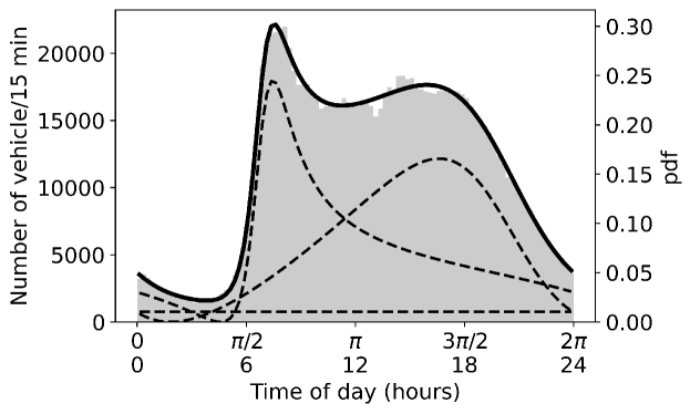
The optimization is carried out for 10,000 initial values. Fig. 3 and Table 1 show the best result among 10,000 estimations. Table 2 provides the values of the empirical and theoretical trigonometric moments. The solid line in Fig. 3 represents the estimated density of the mixture and the dashed lines refer to the estimated densities of the components. The same convention will be used in the following figures of fitted densities. The value of ETM is $7.06\times 10^{-13}$ and that of the log-likelihood function is $-$1,840,939. As shown in the right column of Table 2, the difference between the values of empirical and theoretical trigonometric moments of all the degrees are approximately 0, which means that this result is very close to the result of ordinary method of moments estimation. Nonetheless, we generally need the proposed modified method of moments to ensure that the parameters are within their ranges, as explained in Section 4.2. Actually, when the number of components $m$ is set to be greater than two, much larger values of ETM are obtained for some cases and the ordinary method of moments estimates are out of range for some parameters (see Section 6.2). Also, the estimated densities in Fig. 3 fit fairly well to the histogram. The sharp and negatively skewed peak around $\pi/2$ is represented by the component with $k=1$, while the gentle peak around $3\pi/2$ is modelled by the component with $k=2$.

The computation time for 10,000 trials is about 300 sec. The calculation was run on a Windows 10 computer with an Intel Core i7-8700 processor running at 3.20 GHz using 32.0 GB of RAM. Furthermore, about 25% of 10,000 trials converge to a similar value to this best result. This implies that we can obtain the optimum parameters by starting estimation with a feasible number of initial values at least in this case. We confirmed that various initial values reached the estimated parameters close to those in Table 1 and the initial value in Table 1 is just an example of such initial values.

5.2 Maximum likelihood estimation

The EM algorithm is carried out by setting the initial values as the best estimates from the modified method of moments to achieve the maximum likelihood estimation. This choice of the initial values seems reasonable because of the large sample size of the data and the consistency of the modified method of moments estimator and maximum likelihood estimator. For numerical optimization in the M-step, namely, Step 2 in Algorithm 4.1, the same python package as in the optimization of ETM is employed. In this analysis, each M-step is terminated when the difference of the value of the objective function between two successive iterations is lower than $1\times 10^{-6}$. Also, the whole EM algorithm is terminated when the difference of the log-likelihood function between two successive M-steps is lower than 1. This threshold is set by the following reasoning. Since the number of samples in this study is more than 1,000,000, the absolute value of the log-likelihood function is expected to be of that order of magnitude. Thus, we regard the threshold 1 as small enough to claim convergence.

Figure 4: Plot of the densities of the reparametrized mixture (5) (bold) and its components (dashed) estimated via the EM algorithm.

Table 3: Parameter estimates associated with the maximum likelihood estimation for the reparametrized mixture (5) via the EM algorithm.

$k$ $\hat{\mu}_{k}$ $\hat{\rho}_{k}$ $\hat{\lambda}_{k}$ $\hat{\pi}_{k}^{\prime}$ 1 2.7572 0.7266 5.3136 0.4536 2 4.0107 0.1970 1.1895 0.4825 3 0.0639

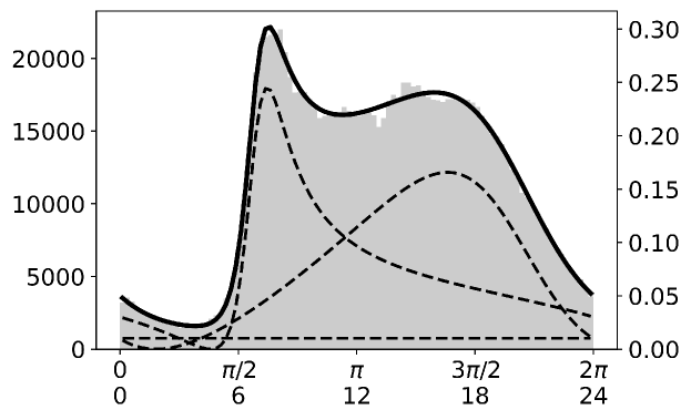
The result of the EM algorithm is shown in Fig. 4 and Table 3. It takes just two steps to terminate the EM algorithm. The value of ETM increases along with that of the log-likelihood during the EM algorithm. The difference between the parameter estimates by the modified method of moments and those by the maximum likelihood estimation is not much. This implies that the modified method of moments estimate is close to the MLE, the estimate produced by another consistent estimator.

As for the computation time, it takes 899 sec. for the EM algorithm although only two M-steps are conducted in the calculation. The calculation environment is the same as that of the previous subsection. Compared to the modified method of moments that takes only about 300 sec. for 10,000 trials, the EM algorithm requires a much longer time. Therefore, setting the initial value close to the maximum likelihood estimator is necessary to achieve the maximum likelihood estimation by the EM algorithm in a feasible computation time. The proposed modified method of moments is one possible solution for this purpose.

Figure 5: Plot of the estimated densities of the recovered mixture (1) (bold) and their components (dashed).

Table 4: Maximum likelihood estimates for the mixture with the recovered original parametrization (1).

$k$ $\hat{\mu}_{k}$ $\hat{\gamma}_{k}$ $\hat{\rho}_{k}$ $\hat{\lambda}_{k}$ $\hat{\pi}_{k}$ 1 2.7572 0.3751 0.7267 5.3136 0.4845 2 4.0107 0.4855 0.1970 1.1895 0.5155

Here, the parameters are estimated in the form of the mixture of two Kato–Jones distributions and the uniform distribution (Table 3(b) and equation (4)). Actually, we can regard this mixture of three components as the estimated model. Nonetheless, we are also able to reparameterize and recover the estimates of the original parameters (1) as discussed in Section 4.1. As we initially aim to estimate the mixture of two components, we employ the latter in the following. The maximum likelihood estimates obtained via the EM algorithm (Fig. 4 and Table 3) are recovered to ${\hat{\mu}_{k},\hat{\gamma}_{k},\hat{\rho}_{k},\hat{\lambda}}_{k}$ and ${\hat{\pi}}_{k}$ as shown in Fig. 5 and Table 4. Then, the recovered parameters are reparameterized into $\hat{\bar{\alpha}}_{2k}$ and $\hat{\bar{\beta}}_{2k}$ as shown in Table 5. The shapes of the two estimated components with $k=1,2$ in Table 3 slightly change by adding the restored uniform component with $k=3$.

Table 5: Maximum likelihood estimates for the reparametrized mixture (3).

$k$ $\hat{\mu}_{k}$ $\hat{\gamma}_{k}$ $\hat{\bar{\alpha}}_{2k}$ $\hat{\bar{\beta}}_{2k}$ $\hat{\pi}_{k}$ 1 2.7572 0.3751 0.1542 -0.2248 0.4845 2 4.0107 0.4855 0.0356 0.0888 0.5155

5.3 Discussion

Here we discuss the interpretation of the estimated models with the recovered parametrizations (1) and (3) given in Tables 4 and 5, respectively. As $\hat{\pi}_{1}$ and $\hat{\pi}_{2}$ have similar values, the weights of these components are approximately the same. Next, the peak of the component with $k=1$ is sharp and negatively skewed. Its mean, $\hat{\mu}_{1}$, is around 10:32 and its mode is around 7:28 (Kato and Jones, 2015, Supplementary Material). The shape is characterized by large $\hat{\bar{\alpha}}_{21}$ and negatively large $\hat{\bar{\beta}}_{21}$. As explained in Section 2, this result is consistent with the actual situation that many drivers would like to arrive in central Osaka at just around the same time like 8:30 and 9:00. On the other hand, the peak of the component with $k=2$ is gentle and positively skewed. Its mean, $\hat{\mu}_{2}$, is around 15:19 and its mode is around 16:37. The shape is characterized by small $\hat{\bar{\alpha}}_{22}$ and positively small $\hat{\bar{\beta}}_{22}$. The result shows that evening traffic flow does not concentrate in a short time compared with the morning one. This may be because drivers do not have to leave their office at the same time, which is different from morning hours. Perhaps, some of them decide to make their departure time earlier or later than peak hour to avoid traffic congestion. In addition, the positively skewed shape may imply that they also avoid being too late returning home.

These interpretations are made by focusing on the shape around the mode of each peak. It is more difficult to understand the traffic flow volume around the tails of both components. For example, the first component still has a moderate probability at around 16:00, which cannot be included in the morning rush hour. One possible explanation is that the first component represents the first trip of the day that includes the morning commuting. While others make their first trip in the evening because they work at nighttime or they go shopping. Especially, people who work at night are more likely to use their own vehicles for commuting than those who work in the daytime as public transport is not operating after midnight. This could be an explanation for the first component having larger probability than the second component after around 22:00. Similarly, the second component represents the second and subsequent trips of the day that include the evening commuting. As round and migration trips during daytime, for example, may be included in the second component, it already has a moderate value even in the morning hours. Nonetheless, further investigation is necessary for more detailed analyses, e.g., considering the effect of commercial trips and heavy vehicles by changing the number of components.

6 Comparison with other models

We compare other multimodal distributions with our proposed model in terms of practicability and fit.

6.1 Mixture of von Mises distributions

First, we employ the mixture of von Mises (MovM) distributions with density

$$f(\theta)=\sum_{k=1}^{m}\frac{\pi_{k}}{2\pi I_{0}(\kappa_{k})}\exp(\kappa_{k}\cos(\theta-\mu_{k})),\quad 0\leq\theta<2\pi{\color[rgb]{0,0,0},}$$

where $\mu\in[0,2\pi)$ is the mean direction, $\kappa\in[0,\infty)$ is a concentration parameter, $I_{0}(\cdot)$ is the modified Bessel function of the first kind and order zero, $m\in\mathbb{N}$ is the number of components of the mixture and $0<\pi_{1},\ldots,\pi_{m}<1$ are the weights of the components satisfying $\sum_{k=1}^{m}\pi_{k}=1$. This distribution is one of the most popular multimodal directional distributions (e.g., Wallace and Dowe, 2000; Mooney et al., 2003; Banerjee et al., 2005; Mulder et al., 2020). The number of components is set to two as in our proposed model.

Figure 6: Plot of the estimated MovM distribution.

Table 6: Maximum likelihood estimates of the parameters of the MovM distribution.

$k$ $\hat{\mu}_{k}$ $\hat{\kappa}_{k}$ $\hat{\pi}_{k}$ 1 2.1858 6.8060 0.2393 2 4.1274 1.0975 0.7607

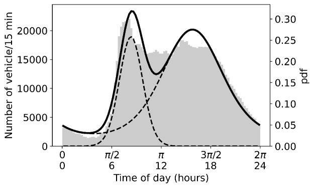
Maximum likelihood estimation is achieved by the EM algorithm as shown in Fig. 6 and Table 6. The value of the log-likelihood function is $-$1,852,948, which is worse than that of our model ($-$1,840,917). Comparison between Figs. 4 and 6 suggests that the fit of the MovM distribution is not as good as that of our model. In particular, as MovM cannot control the skewness and kurtosis of the component distributions, the negatively skewed peak around 7:00 and gentle peak around 16:00 cannot be modelled successfully.

6.2 Our mixture with more than two components

We estimate the mixed Kato–Jones distributions (3) whose number of components $m$ is more than two. In this subsection, models with $m\leq 6$ are discussed because of stability of estimation; estimation for the model with $m>6$ was carried out but the results were unstable. Recall that the histogram shows two peaks that can be interpreted as shown above and the assumption of more than two peaks is not necessarily insightful from the transport engineering viewpoint. As such, the main purpose of this subsection is not to find the most accurate number of components but to find out what shapes of distributions will be obtained.

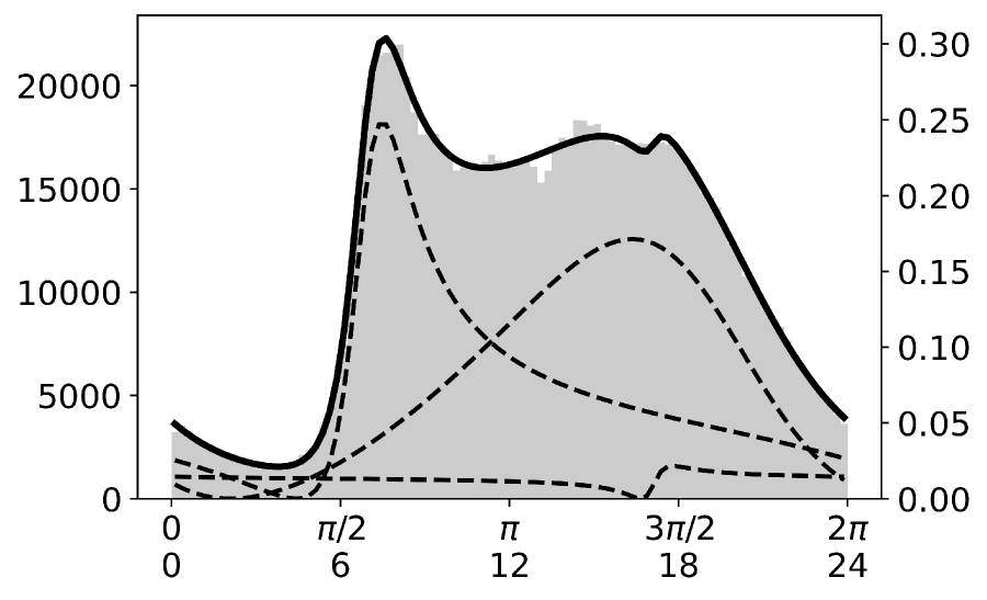
The conditions for the estimation are the same as those in Section 5. Table 7 shows the estimated values of ETM by the proposed method for each $m$. The estimated value of ETM for $m=2$ is much smaller than that for $m\geq 3$. This result implies that the solutions to the estimating equations for the (ordinary) method of moments do not exist within the range of parameters for $m\geq 3$. The proposed method, the modified method of moments, has the advantage that it can avoid this problem regardless of the value of $m$. Fig. 7 and Table 8 show the results of maximum likelihood estimation for the mixtures with $m=3,\ldots,6$.

Table 7: The values of ETM for the modified method of moments estimates associated with $m$ components.

$m=2$ $m=3$ $m=4$ $m=5$ $m=6$ $5.70\times 10^{-14}$ $9.66\times 10^{-6}$ $4.89\times 10^{-6}$ $2.14\times 10^{-6}$ $3.46\times 10^{-7}$

Figure 7: Panels from (a) to (d) show maximum likelihood fits of the densities with the numbers of components $m$ from 3 to 6, respectively.

Table 8: Maximum likelihood estimates of the parameters of Kato–Jones mixtures (3) whose numbers of components $m$ are from 3 to 6.

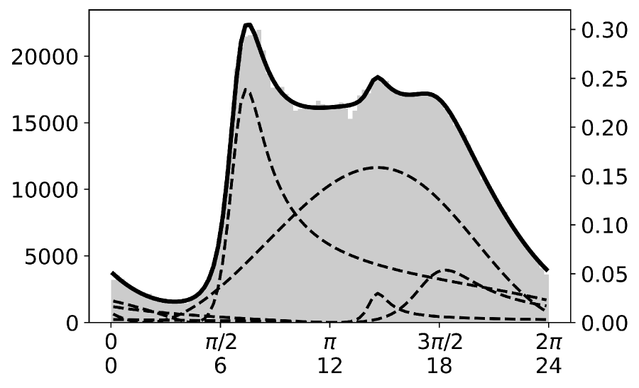
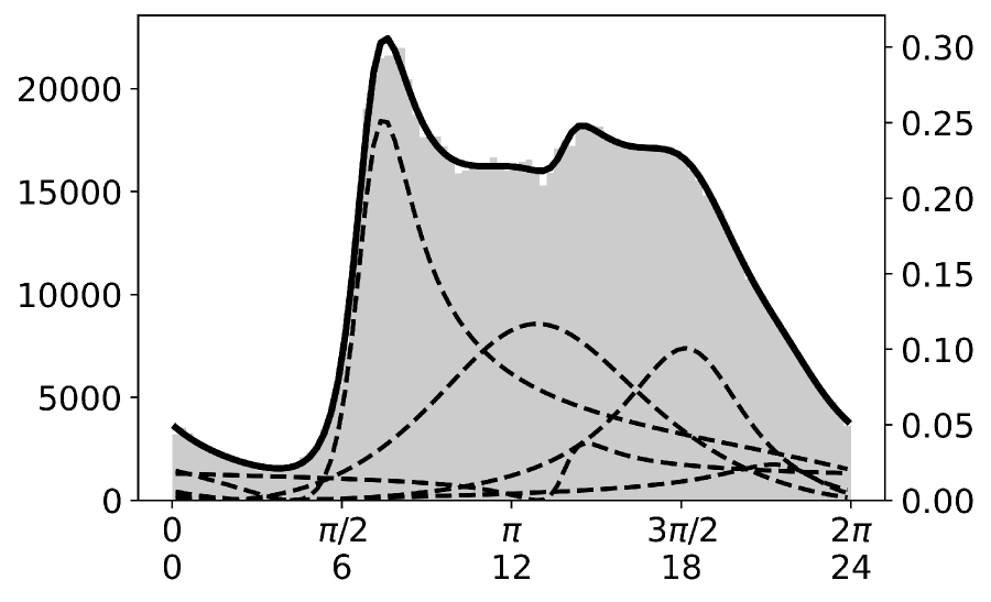
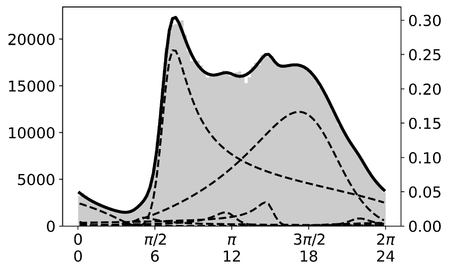
$m$ $k$ $\hat{\mu}_{k}$ $\hat{\gamma}_{k}$ ${\hat{\bar{\alpha_{2}}}}_{k}$ ${\hat{\bar{\beta_{2}}}}_{k}$ $\hat{\pi}_{k}$ $m=3$ 1 2.7174 0.4289 0.1881 -0.2449 0.4387 2 4.0189 0.5422 0.0591 0.0802 0.4795 3 6.2832 0.1025 0.0209 0.0864 0.0818 $m=4$ 1 2.6665 0.4376 0.2128 -0.2452 0.3855 2 3.7380 0.5065 0.0076 0.0225 0.4907 3 4.3642 0.4887 0.3402 -0.2284 0.0285 4 5.2889 0.6037 0.2628 -0.2166 0.0952 $m=5$ 1 2.6404 0.4696 0.2312 -0.2488 0.4025 2 3.4376 0.6195 0.1491 -0.0229 0.2788 3 4.5981 0.7240 0.3421 0.0824 0.1668 4 5.0203 0.5727 0.2377 0.2275 0.0437 5 5.0969 0.1971 0.0174 -0.1568 0.1082 $m=6$ 1 2.0184 0.4581 0.2523 -0.2446 0.0175 2 2.5605 0.6225 0.4042 0.2344 0.0221 3 2.7815 0.3914 0.1555 -0.2382 0.4875 4 3.0897 0.3797 0.2054 0.2274 0.0499 5 4.1662 0.5756 0.1201 0.1227 0.4139 6 5.8877 0.8428 0.6246 -0.1011 0.0091

In the results of $m=3$ shown in Fig. 7(a) and Table 8, there are two prominent components with $k=1,2$ that have large values of $\hat{\pi}_{k}$. They are similar to the two components in the result of $m=2$ in terms of both the values of parameters and the shapes of the curves (see Table 4). The component with $k=3$ has a small value of $\hat{\pi}_{3}$ and represents the small peak around 16:00 seen in the histogram, which results in the mode of the component with $k=3$ at 17:47. This result shows that the three-component mixture brings about almost the same result as the two-component one. The additional component to $m=2$ may not be meaningful from the transport engineering viewpoint; it only represents the trivial peak along with the improvement of the value of the log-likelihood function.

This tendency is also true for the cases of $m>3$. Two of their components have relatively large values of $\hat{\pi}_{k}$ that represent two main peaks in the result of $m=2$: morning and evening peaks. The other components have small values of $\hat{\pi}_{k}$ that represent small peaks. The interpretation of the parameters for these small components is difficult.

Figure 8: Panels from (a) to (e) display the plots of the values of the log-likelihood function, AIC, BIC, the computation time for the optimization of ETM and the computation time for the EM algorithm for the numbers of components $m$ from 2 to 6, respectively.

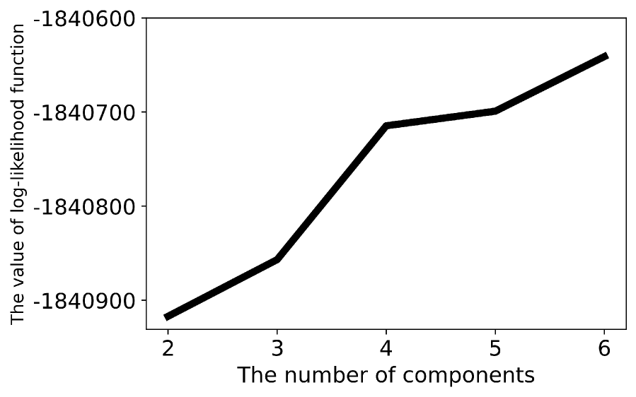
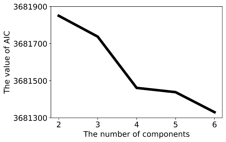
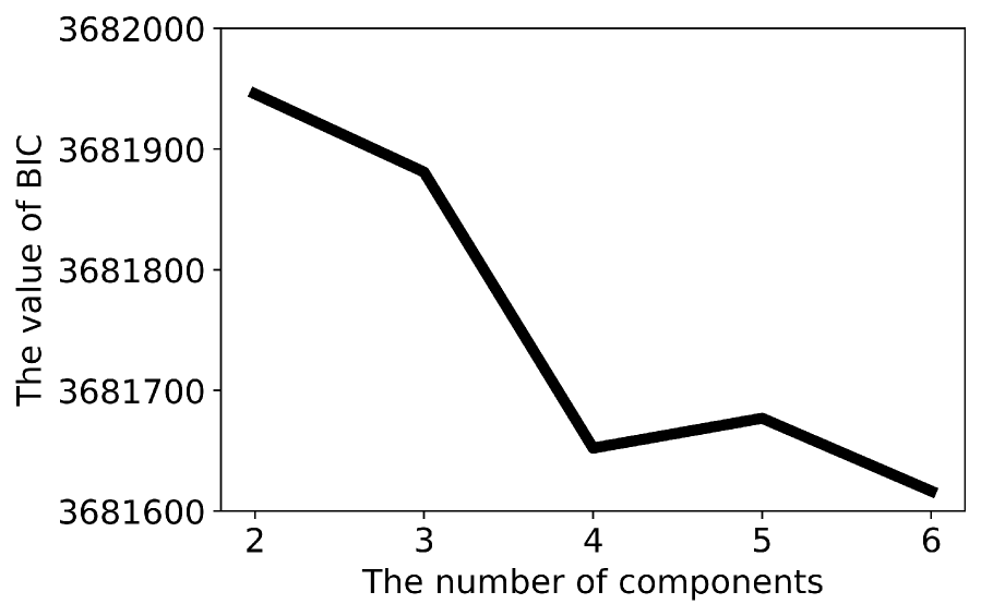
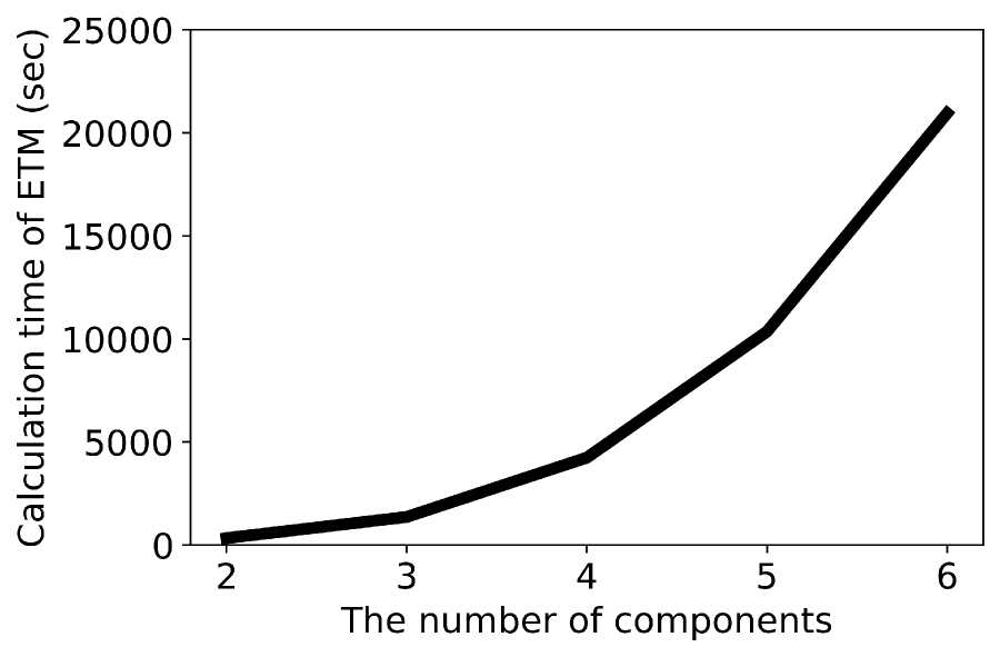
Fig. 8 shows the values of the log-likelihood function, AIC, BIC, the computation time for the optimization of ETM, and that for the EM algorithm, as functions of the number of components $m$. The value of the log-likelihood function increases as $m$ increases for $m\leq 6$ (Fig. 8(a)). In addition, Fig. 8(b) and (c) imply that the values of AIC and BIC are monotonically decreasing with respect to $m$ except for that of BIC for $m=5$. In these senses, the model with $m=6$ is preferable. Two prominent components and four small components are seen in this model. Fig. 7(d) and Table 8 show that the components with $k=3$ and $k=5$ represent the morning and evening peaks, respectively. The other components with $k=1,2,4,6$ model small peaks on the histogram, which are difficult to interpret, and their modes are at 5:11, 11:30, 14:38 and 21:58, respectively. Unsurprisingly, larger $m$ needs a longer computation time (Fig. 8(d) and (e)) as the optimization problem becomes more complicated.

Further consideration of determining the appropriate number of components may be necessary. The values of AIC and BIC suggest a larger number of components. The small components seen in these cases might be generated by some unknown factors and phenomena. Nonetheless, from the viewpoints of interpretability of the result and feasibility of the calculation, we regard $m=2$ as the most reasonable numbers of components in this study.

7 Simulation study

We compare the performance of the modified method of moments estimation and the maximum likelihood estimation by EM algorithm via a Monte Carlo simulation study. Random samples of sizes $n=50,100,500,1000,$ and $5000$ were generated from the estimated distribution whose parameters are shown in Table 3 (b). For each sample size, $r=2000$ samples were generated.

For comparison of the two estimators, we employ the generalized mean squared error which is defined by $\det{(\Sigma)}$, where $\Sigma=E\{(\hat{\xi}-\xi)(\hat{\xi}-\xi)^{T}\}$ and $\hat{\xi}$ is an estimator of $\xi=(\mu_{1},\mu_{2},\rho_{1},\rho_{2},\lambda_{1},\lambda_{2},\pi^{\prime}_{1},\pi^{\prime}_{2})^{T}$. An estimate of the generalized mean squared error is given by replacing $\Sigma$ by its sample analogue $\hat{\Sigma}=r^{-1}\sum^{r}_{j=1}{(\hat{\xi}_{j}-\xi)(\hat{\xi}_{j}-\xi)^{T}}$, where the $\hat{\xi}_{j}$’s, $j=1,...,r$, are the estimates from the $r$ simulation samples. We also consider the estimated relative generalized mean squared error of the estimate via the modified method of moments with respect to the maximum likelihood estimate, which is defined as

$$\widehat{\rm{RGMSE}}=\frac{\det{(\hat{\Sigma}_{MM}})}{\det{(\hat{\Sigma}_{ML}})}{\color[rgb]{0,0,0}.}$$

Here, $\hat{\Sigma}_{MM}$ and $\hat{\Sigma}_{ML}$ are sample estimates of the mean squared error matrices of modified method of moments estimation and maximum likelihood estimation, respectively. The conditions of the modified method of moments estimation are the same as in the previous section except for the number of initial values, which is set to 100 in this simulation. Maximum likelihood estimation is achieved by the EM algorithm, whose initial value is the modified method of moments estimate and the threshold of termination for the EM algorithm is set to $n\times 10^{-6}$. In both estimates, it is assumed that $\hat{\mu}_{1}<\hat{\mu}_{2}$.

Table 9: The values of $\det{(\hat{\Sigma}_{MM})}$, $\det{(\hat{\Sigma}_{ML})}$ and $\widehat{\rm{RGMSE}}$

$n$ $n=50$ $n=100$ $n=500$ $n=1000$ $n=5000$ $\det{(\hat{\Sigma}_{MM})}$ $5.35\times 10^{-9}$ $7.00\times 10^{-10}$ $2.70\times 10^{-13}$ $4.25\times 10^{-15}$ $4.01\times 10^{-20}$ $\det{(\hat{\Sigma}_{ML})}$ $5.05\times 10^{-8}$ $6.41\times 10^{-9}$ $3.56\times 10^{-12}$ $1.33\times 10^{-14}$ $1.23\times 10^{-22}$ $\widehat{\rm{RGMSE}}$ 0.106 0.109 0.076 0.322 325.3

Table 9 shows the value of $\det{(\hat{\Sigma}_{MM})}$, $\det{(\hat{\Sigma}_{ML})}$ and $\widehat{\rm{RGMSE}}$ for each sample size. As the number of samples $n$ increases, the value of $\det{(\hat{\Sigma}_{MM})}$ and $\det{(\hat{\Sigma}_{ML})}$ decreases. In addition, as $n$ increases, the value of $\widehat{\rm{RGMSE}}$ also increases. Furthermore, the values of $\widehat{\rm{RGMSE}}$ are smaller than 1 for $n\leq 1000$ and larger for $n=5000$. Therefore, in terms of $\widehat{\rm{RGMSE}}$, modified moments estimation is preferable for estimation from a small number of samples. On the other hand, maximum likelihood estimation is preferable for estimation from a large number of samples such as the data in this paper. Note that modified moments estimation yields not only an estimate but also a good initial value for maximum likelihood estimation. Although the value of $\widehat{\rm RGMSE}$ is relatively large for $n=5000$, the very small value of $\det{(\hat{\Sigma}_{MM})}$ for $n=5000$ indicates that the estimate via the modified moments estimation still has reasonable performance as the initial value for maximum likelihood estimation. Therefore, modified moments estimation is useful to obtain the maximum likelihood estimates efficiently for a large sample size as well as small and medium sample sizes.

It is noted that this result is similar to that of $\widehat{\rm{RGMSE}}$ of the method of moments relative to maximum likelihood estimation for the unimodal Kato–Jones distribution (Kato and Jones, 2015, Supplementary Material).

8 Conclusion

In this paper, we estimated the probability distribution of the variation of traffic volume within an average weekday. We employed the mixture of Kato–Jones distributions, which can provide a wide range of skewness and kurtosis for each component. To estimate the parameters of these distributions, we developed the modified method of moments. This method ensures that the estimated parameters always belong to the parameter space. Then the maximum likelihood method for the proposed mixture was established using the EM algorithm.

The proposed method was applied to some traffic counter data from Japan. As a result, the data were classified into two components, which were interpreted as the morning and evening traffic. Some reasonable explanations for these components are suggested, that the difference in the shapes of the components might be caused by the different behaviours underlying the commuting trips between morning and evening hours. In addition, the modified method of moments was seen to allow for fast calculation and provided a reasonable initial value for maximum likelihood estimation. With this initial value, the EM algorithm provided reasonable maximum likelihood estimates.

According to information criteria such as $AIC$ and $BIC$, a larger number of components than two resulted in better estimation. However, the interpretation of these models is difficult thus far. As future work, it would be interesting to consider other methods for model selection based on cross validation or information criteria with a restricted parameter space. In addition, further consideration of missing factors that generate third and later components may be necessary. Some additional information such as each vehicle’s origin, destination, and trip purpose would be useful for this.

Appendix A. Proof of Theorem 1

The $p$th trigonometric moment of a random variable $\Theta$ following the Kato–Jones distribution (2) is $\phi_{\rm KJ}(p)\equiv E(e^{ip\Theta})=\gamma\,(\rho e^{i\lambda})^{-1}\left\{\rho e^{i(\mu+\lambda)}\right\}^{p}$ (Kato and Jones, 2015). For convenience, we reparametrize the Kato–Jones distribution (2) via $\alpha=-\lambda$, $\beta=\gamma/\rho$ and $\eta=\mu+\lambda$. Then we have $\phi_{\rm KJ}(p)=\beta e^{i\alpha}\left(\rho e^{i\eta}\right)^{p}$.

The $p$th trigonometric moment of a random variable having the density $h_{j}$ is given by $\phi_{h_{j}}(p)=\int_{-\pi}^{\pi}e^{ip\theta}h_{j}(\theta)d\theta{\color[rgb]{0,0,0}\ =e^{ip\mu_{j}}\int_{-\pi}^{\pi}e^{ip(\theta-\mu_{j})}h_{j}(\theta)d\theta}=\xi_{j,p}e^{ip\mu_{j}}$, where $\xi_{j,p}=E[\cos\{p(\theta-\mu_{j})\}]$. It follows from the assumption that $\xi_{j,p}>0$ for any $p\in\mathbb{Z}^{+}$. We show that, if

$$\phi_{\rm KJ}(p)=\pi_{1}\phi_{h_{j}}(p)+\pi_{2}\phi_{h_{j}}(p),$$

then $\alpha=0$ or $\pi$. Taking arguments of both sides of this equation, we have

$$\alpha+p\eta=\arg\left\{\pi_{1}\xi_{1,p}e^{ip\mu_{1}}+\pi_{2}\xi_{2,p}e^{ip\mu_{2}}\right\},\quad p\in\mathbb{Z}^{+}.$$

This implies that, for any $p\in\mathbb{Z}^{+}$,

$$\pi_{1}\xi_{1,p}\sin\{p(\mu_{1}-\eta)-\alpha\}+\pi_{2}\xi_{2,p}\sin\{p(\mu_{2}-\eta)-\alpha\}=0.$$ (S1)

It follows from this expression and $\pi_{1},\pi_{2},\xi_{1,p},\xi_{2,p}>0$ that

$$\sin\{p(\mu_{1}-\eta)-\alpha\}\sin\{p(\mu_{2}-\eta)-\alpha\}\leq 0,\quad p\in\mathbb{Z}^{+}.$$ (S2)

The left-hand side of the inequality (S2) can be expressed as

$$\sin\{p(\mu_{1}-\eta)-\alpha\}\sin\{-\{p(\mu_{1}-\eta)-\alpha\}+pc-2\alpha\},$$

where $c=\mu_{1}+\mu_{2}-2\eta$. This expression implies that, if $c\neq 0$, there exists $p\in\mathbb{Z}^{+}$ such that the inequality (S2) does not hold. Then we have $\mu_{2}-\eta=-(\mu_{1}-\eta)$. Thus it follows from equation (S1) that $\alpha=-\lambda=0$ or $\pi$, which corresponds to the symmetric case of the Kato–Jones distribution. $\Box$

Appendix B. Proof of Proposition 1

First we show (i). The parameter space of the Kato–Jones distribution (2) can be expressed as

$$-\pi\leq\mu,\lambda<\pi,\quad 0\leq\rho<1,\quad 0\leq\gamma\leq\frac{1+\rho}{2},\quad\rho\gamma\cos\lambda\geq\frac{\rho^{2}+2\gamma-1}{2}.$$

This parameter space is equivalent to

$$-\pi\leq\mu,\lambda<\pi,\quad 0\leq\rho<1,\quad 0\leq\gamma\leq\frac{1-\rho^{2}}{2(1-\rho\cos\lambda)}.$$

This expression for the parameter space implies that, for given $\rho$ and $\lambda$, $\bar{\gamma}=(1-\rho^{2})/\{2(1-\rho\cos\lambda)\}$ achieves the upper bound of the range of $\gamma$. Using $\overline{\gamma}$, the Kato–Jones density (2) can be written as

$$g_{\rm KJ}(\theta;\mu,\gamma,\rho,\lambda)$$

$$=\frac{\gamma}{\bar{\gamma}}\cdot\frac{1}{2\pi}\left\{1+2\bar{\gamma}\,\frac{\cos(\theta-\mu)-\rho\cos\lambda}{1+\rho^{2}-2\rho\cos(\theta-\mu-\lambda)}\right\}+\left(1-\frac{\gamma}{\bar{\gamma}}\right)\frac{1}{2\pi}$$

$$=\pi^{\prime}\cdot\frac{1}{2\pi}\left\{1+2\bar{\gamma}\,\frac{\cos(\theta-\mu)-\rho\cos\lambda}{1+\rho^{2}-2\rho\cos(\theta-\mu-\lambda)}\right\}+\left(1-\pi^{\prime}\right)\frac{1}{2\pi},$$

as required. It is straightforward to show (ii) by substituting expression (4) into the mixture density (1). $\Box$

References

- Anacleto et al. (2013) Anacleto, O., Queen, C. and Albers, C. J. (2013). Multivariate forecasting of road traffic flows in the presence of heteroscedasticity and measurement errors. Journal of the Royal Statistical Society: Series C (Applied Statistics), 62, 251–270.
- Banerjee et al. (2005) Banerjee, A., Dhillon, I.S., Ghosh, J. and Sra, S. (2005). Clustering on the unit hypersphere using von Mises–Fisher distributions. Journal of Machine Learning Research, 6, 1345–1382.
- Batschelet (1981) Batschelet, E. (1981). Circular Statistics in Biology. London: Academic Press.
- Chen et al. (2010) Chen, X., Li, L. and Zhang, Y. (2010). A Markov model for headway/spacing distribution of road traffic. IEEE Transactions on Intelligent Transportation Systems, 11, 773–785.
- Daganzo (1997) Daganzo, C. F. (1997). Fundamentals of transportation and traffic operations. Pergamon Oxford.
- Edie (1963) Edie, L.C. (1963). Discussion of traffic stream measurements and definitions. Port of New York Authority.
- Hampel et al. (1986) Hampel, F.R., Ronchetti. E.M., Rousseeuw, P.J. and Stahel, W.A. (1986). Robust Statistics, The Approach Based on Influence Functions. New York: Wiley.
- Jones et al. (2001) Jones, E., Oliphant, T., and Peterson, P. (2001). SciPy: Open source scientific tools for Python. (Available from http://www.scipy.org/)
- Kato and Jones (2015) Kato, S. and Jones, M.C. (2015). A tractable and interpretable four-parameter family of unimodal distributions on the circle. Biometrika, 102, 181–190.
- Kraft (1988) Kraft, D. (1988). A software package for sequential quadratic programming. (Available from http://www.opengrey.eu/item/display/10068/147127)
- Leduc (2008) Leduc, G. (2008). Road traffic data: Collection methods and applications. Working Papers on Energy, Transport and Climate Change.
- Ley et al. (2021) Ley, C., Babić, S. and Craens, D. (2021). Flexible models for complex data with applications. Annual Review of Statistics and Its Application, 8, 369–391.
- Li and Chen (2017) Li, L. and Chen, X. M. (2017). Vehicle headway modeling and its inferences in macroscopic/microscopic traffic flow theory: A survey. Transportation Research Part C: Emerging Technologies, 76, 170–188.
- McLachlan and Krishnan (2007) McLachlan, G.J. and Krishnan, T. (2007). The EM Algorithm and Extensions, 2nd ed. Hoboken: Wiley.
- Miyata et al. (2020) Miyata, Y., Shiohama, T. and Abe, T. (2020). Estimation of finite mixture models of skew-symmetric circular distributions. Metrika, 83, 895–922.
- Mooney et al. (2003) Mooney, J.A., Helms, P.J. and Jolliffe, I.T. (2003). Fitting mixtures of von Mises distributions: a case study involving sudden infant death syndrome. Computational Statistics & Data Analysis, 41, 505–513.
- Mulder et al. (2020) Mulder, K., Jongsma, P. and Klugkist, I. (2020). Bayesian inference for mixtures of von Mises distributions using reversible jump MCMC sampler. Journal of Statistical Computation and Simulation, 90, 1539–1556.
- Muñoz et al. (2003) Muñoz, L., Sun, X., Horowitz, R. and Alvarez, L. (2003). Traffic density estimation with the cell transmission model. In Proceedings of the 2003 American Control Conference, 5, 3750–3755.
- Na and Jang (2011) Na, J. H. and Jang, Y. M. (2011). Modeling on daily traffic volume of local state road using circular mixture distributions. The Korean Journal of Applied Statistics, 24, 547–557.
- Nagasaki et al. (2019) Nagasaki, K., Nakanishi, W. and Asakura, Y. (2019). Application of Rose Diagram to Road Network Analysis. In Proceedings of 24th International Conference of Hong Kong Society for Transportation Studies, 169–176.
- Pewsey and García-Portugués (to appear) Pewsey, A. & García-Portugués, E. Recent advances in directional statistics. Test, to appear.
- Press (1972) Press, S.J. (1972). Estimation in univariate and multivariate stable distributions. Journal of the American Statistical Association, 67, 842–846.
- Transportation Research Board (2010) Transportation Research Board (2010). Highway capacity manual. National Research Council, Washington, DC.
- Wallace and Dowe (2000) Wallace, C.S. and Dowe, D.L. (2003). MML clustering of multi-state, Poisson, von Mises circular and Gaussian distributions. Statistics and Computing, 10, 73–83.
- Wang and Papageorgiou (2005) Wang, Y. and Papageorgiou, M. (2005). Real-time freeway traffic state estimation based on extended Kalman filter: a general approach. Transportation Research Part B: Methodological, 39, 141–167.