Formal Analysis of Lending Pools in Decentralized Finance

Abstract

Decentralised Finance (DeFi) applications constitute an entire financial ecosystem deployed on blockchains. Such applications are based on complex protocols and incentive mechanisms whose financial safety is hard to determine. Besides, their adoption is rapidly growing, hence imperilling an increasingly higher amount of assets. Therefore, accurate formalisation and verification of DeFi applications is essential to assess their safety. We have developed a tool for the formal analysis of one of the most widespread DeFi applications: Lending Pools (LP). This was achieved by leveraging an existing formal model for LPs, the Maude verification environment and the MultiVeStA statistical analyser. The tool supports several analyses including reachability analysis, LTL model checking and statistical model checking. In this paper we show how the tool can be used to analyse several parameters of LPs that are fundamental to assess and predict their behaviour. In particular, we use statistical analysis to search for threshold and reward parameters that minimize the risk of unrecoverable loans.

1 Introduction

Financial trading has recently shifted to virtual markets, platforms entirely regulated and controlled by novel protocols. Decentralised Finance (DeFi) [34] applications are deployed on blockchains like Ethereum [34, 12], which offer distributed infrastructures to execute smart contracts [18] without intermediaries. DeFi has recently been employed by a growing community of users. As of April 2022, the growth of the capital locked by DeFi applications has increased almost $10$ times in the last two years: from approximately $9.78bn, on 1 April 2020, to over $83.51bn, on 1 April 2022 [29]. Even assuming the security guarantees ensured by the underlying blockchain, DeFi smart contracts have several vulnerabilities latent in their design [30, 36]. Given the considerable amount of funds daily exchanged on DeFi platforms [1, 16], even minor design flaws could determine massive and intolerable losses [21]. Notwithstanding the increasing interest of several research groups in this area [9, 5, 2, 32, 4, 19], the complexity of DeFi protocols yields new interesting research problems. Formal verification of these systems is crucial, in order to ensure their correctness and security.

The verification tool proposed in this paper simulates and analyses Lending Pools (LPs), one of the most popular DeFi applications, whose two main features are lending and borrowing assets, to support various financial practices, including margin trading. Our verification tool is based on the formal model of LPs proposed in [6]. Such model encompasses the behaviour of the most widespread LPs, namely Aave [10] and Compound [24].

We craft an operational specification of the LP model of [6] in Maude [15], a specification language which is particularly suitable for highly concurrent systems such as LPs. Additionally, Maude provides a very extensive environment for both simulating and verifying the properties of the specified models. Given the complexity of the modelled systems, the analyses techniques offered by the Maude environment are not sufficient. Specifically, since the system may evolve by following an infinite number of execution paths, the traditional model checking methods result in being either ineffective or unviable. Therefore, the Maude-based LP simulator has been extended to support statistical analyses. This has been achieved by integrating the simulator with the MultiVeStA statistical analyser proposed in [31] and recently redesigned to focus on analyses of interest for of economical agent-based models [33]. The tool offers analysis techniques from the family of statistical model checking [3]. These statistical analyses, despite producing less accurate results, allow to observe the quantitative behaviour of large instances of the model, offering statistically-reliable results. In the case of lending pools, this approach allows to estimate parameters of the model so to increase its safety. Specifically, an essential safety property of the model is that the value of non-repayable loans is low.

This paper is based on the work done in [25] and proposes a Maude-based LP simulator (Section 3) capable of conducting several analyses of lending pools including LTL model checking and statistical analysis. The tool is open source and available at [26]. Additionally, the study showcases the usage of the tool by answering a still non-investigated research question, aiming at an enhancement of the analysed platforms’ safety. In particular, the statistical analysis presented in Section 4 shows that a choice of the parameters used to instantiate the LP model reduces the amount of non-repayable loans.

2 Lending Pools and Price Models

2.0.1 Lending Pools.

Lending Pools [35] are a class of DeFi applications which allow users to lend and borrow cryptoassets. At the time of writing, LPs are the most used DeFi applications, with the majority of them being deployed on Ethereum [29]. Deposited funds are pooled and lent on-demand to borrowers, only if they possess enough collateral (i.e.  only if their account is overcollaterized). As blockchains typically do not provide strong identities, but pseudonyms [12], users’ actions are difficult to be regulated under a jurisdiction, which makes collateralization the main protection mechanism against adversarial behaviours [27]: an agent can only borrow a quantity of tokens worth less than the amount of collateral they deposited. This mechanism and others (e.g.  interest rates) is in place in order to incentivize borrowers to repay their loans.

We now recall details of the lending pools model in [6]. The basic components of the model are agents and cryptoassets. LP agents are the rational entities taking part in the protocol. Contrarily, LP cryptoassets are token types, each representing a different virtual currency. The model distinguishes two classes of token types: free tokens and minted tokens, denoted respectively by the sets $\mathcal{T}_{f}=\{\tau_{i}\}_{i\in[1..k]}$ and $\mathcal{T}_{m}=\{\tau^{\prime}_{i}\}_{i\in[1..k]}$, where $k$ is the number of cryptocurrencies available on the pool. The difference between these classes of token types is that free tokens have a value established by external markets, whereas minted tokens are assets coined by the protocol, hence holding value only in a specific LP environment. In other words, minted tokens are loyalty credits held by the agents actively joining the protocol. In fact, minted tokens are granted by the protocol to the agents in return for free tokens, hence each minted token $\tau^{\prime}$ corresponds to a free token $\tau$, also called its underlying token. We denote by $\mathcal{T}$ the set of all token types, i.e. $\mathcal{T}=\mathcal{T}_{f}\cup\mathcal{T}_{m}$.

Given agents and assets, the LP model yields as a transition system where each state $\Gamma$ is of the form $\Gamma=\sigma\ |\ \pi\ |\ p$:

1. The wallets function $\sigma:\mathcal{A}\rightarrow(\mathcal{T}\rightarrow\mathbb{R}^{+}_{0})$ stores each agent’s balance of tokens. For instance, the wallet of an agent $\mathit{A}$ is expressed by the partial function $\sigma_{\mathit{A}}$, and the balance of its $\tau$-typed tokens by $\sigma_{\mathit{A}}(\tau)$.

2. The pool component $\pi$ is a triple $(\pi_{f},\pi_{l},\pi_{m})$. It is composed by three partial functions: $\pi_{f}:\mathcal{T}_{f}\rightarrow\mathbb{R}^{+}_{0}$ storing the amount of free tokens deposited in the pool, $\pi_{l}:\mathcal{A}\rightarrow(\mathcal{T}_{f}\rightarrow\mathbb{R}^{+}_{0})$ memorising the loans each agent owes to the pool and $\pi_{m}:\mathcal{T}_{f}\rightarrow(\mathcal{T}_{m}\times\mathbb{R}^{+}_{0})$ keeping track of the minted tokens (also called the collateral or credits) purchased from the pool.

3. The price function $p:dom(\pi_{f})\rightarrow\mathbb{R}^{+}_{0}$ stores the price of each free token available in the pool.

Given a partial map $f$, we denote by $f\{v/x\}$ the point-wise update of $f$ at the point $x$ to the value $v$. In order to add and remove tokens in the functions defined above, a partial binary operation $\circ:\mathbb{R}^{+}_{0}\times\mathbb{R}^{+}_{0}\rightarrow\mathbb{R}^{+}_{0}$, such as addition, is extended to them. Given a partial map $f:\mathcal{T}\rightarrow\mathbb{R}^{+}_{0}$, a token type $\tau\in\mathcal{T}$ and a value $v\in\mathbb{R}^{+}_{0}$, the partial map $f\circ v:\tau$ is defined as

$$f\circ v:\tau=\begin{cases}f\{f(\tau)\circ v/\tau\}\text{ if }\tau\in\mathop{dom}(f)\text{ and }f(\tau)\circ v\text{ is defined}\\ f\{v/\tau\}\mathrm{\ if\ }\tau\notin\mathrm{dom(}f\mathrm{)}\end{cases}$$

In order to describe the model evolution, some additional definitions shall be given. The following LP components may rely on the whole state $\Gamma$, or some of its components. This dependency is indicated by the means of subscripts. For instance, writing $F_{X}$ means that $F$ depends on the $X$ component of the state.

The functions $V_{\Gamma}^{l}$ and $V_{\Gamma}^{m}$ define, respectively, value of tokens lent to a given agent, and the value of minted tokens owned by a given agent:

$$V_{\Gamma}^{l}(\mathit{A})=\sum_{\tau\in\mathcal{T}_{f}}(\pi_{l}(\mathit{A}))(\tau)\cdot p(\tau)\hskip 14.22636ptV_{\Gamma}^{m}(\mathit{A})=\sum_{\tau^{\prime}\in\mathcal{T}_{m}}\sigma_{\mathit{A}}(\tau^{\prime})\cdot\mathit{ER}_{\pi}(\tau^{\prime},\tau)\cdot p(\tau)$$

where $\mathit{ER}_{\pi}(\tau^{\prime},\tau)$ is the exchange rate of minted tokens (see Section 3.1 of [6]).

The collateralization of an agent $\mathit{A}$ is defined as $C_{\Gamma}(\mathit{A})=\nicefrac{{V_{\Gamma}^{m}(\mathit{A})}}{{V_{\Gamma}^{l}(\mathrm{\mathit{A}})}}$. This is an essential indicator of agents’ lending safety: in fact, a collateralization below a given threshold ($C_{\mathrm{min}}$) entails an agent to be liquidated and hence to incur in a financial loss, as detailed later.

The behaviour of agents interacting with a lending pool is formalized as a set of rewriting rules, which define transitions between states. Such transitions are written as $\Gamma\xrightarrow{\mathrm{r_{\mathit{A}}}(z^{n})}\Gamma^{\prime}$, where $\Gamma$ is the starting state, $\Gamma^{\prime}$ is the target state, and $\mathrm{r}_{\mathit{A}}(z^{n})$ is the action (fired by $\mathit{A}$) which triggers the state transition. Actions have the form $\mathrm{r}_{\mathit{A}}(z^{n})$, where $\mathrm{r}$ is the action name, and $z^{n}$ is an $n$-tuple of parameters.

$\mathrm{Dep}_{\mathit{A}}(v:\tau)$	$\mathit{A}$ deposits $v$ free-tokens of type $\tau$ from its wallet to the pool. Subsequently, the pool coins $v^{\prime}$ units of $\tau^{\prime}$, with $v^{\prime}$ computed so to incentivize deposits only if the LP is lacking free tokens.
$\mathrm{Rdm}_{\mathit{A}}(v:\tau^{\prime})$	$\mathit{A}$ redeems $v$ units of the minted token $\tau^{\prime}$, as long as $\mathit{A}$’s collateralization is greater than a threshold ($C_{\mathrm{min}}$) and LP holds enough tokens of type $\tau^{\prime}$.
$\mathrm{Bor}_{\mathit{A}}(v:\tau)$	$\mathit{A}$ borrows $v$ units of a free token $\tau$, assuming it has enough collateral.
$\mathrm{Rep}_{\mathit{A}}(v:\tau)$	$\mathit{A}$ repays $v$ units of its loan in the free token $\tau$ to the LP.
$\mathrm{Liq}_{\mathit{A}}(\mathit{B},v:\hat{\tau},\tau^{\prime})$	$\mathit{A}$ (liquidator) liquidates a variable amount of $\mathit{B}$’s (borrower’s) minted tokens $\tau^{\prime}$, by paying $v$ units of free tokens $\hat{\tau}$. Notably, $\hat{\tau}\in\mathcal{T}_{f}$ is in general different from $\tau$, the underlying token of $\tau^{\prime}\in\mathcal{T}_{m}$. This action can be executed only if the $\mathit{B}$’s collateralization is below $C_{\mathrm{min}}$, meaning $\mathit{B}$ is undercollaterized.
$\mathrm{Int}$	The LP contract accrues interest on the existing loans. This disincentivizes borrowers from postponing their loans repayment.
$\mathrm{Price}$	Token prices are updated according to a given price evolution model.

Table 1: Summary of some of the lending pools actions from [6].

The main actions of lending pools are informally summarised in Table 1. Since the focus in this paper is on liquidations as one of the key incentive mechanisms, we will provide the details for such action only.  Figure 1 provides a formal description of the rule. The essential preconditions to understand the rule are , , , and .

$$\begin{array}[]{l@{\ }l@{\qquad}l@{\ }l@{\qquad}l@{\ }l}\leavevmode\hbox to14.63pt{\vbox to14.63pt{\text{[drawing]}}}&\tau^{\prime}\in\mathcal{T}_{m}&\leavevmode\hbox to14.63pt{\vbox to14.63pt{\text{[drawing]}}}&\sigma_{\mathit{A}}(\hat{\tau})\geq v&\leavevmode\hbox to14.63pt{\vbox to14.63pt{\text{[drawing]}}}&\pi_{l}(\mathit{B})(\hat{\tau})\cdot\textit{Maxliq}\geq v\\ \leavevmode\hbox to14.63pt{\vbox to14.63pt{\text{[drawing]}}}&v^{\prime}=v\cdot\frac{p(\hat{\tau})}{p(\tau)}\cdot r_{\mathrm{liq}}&\leavevmode\hbox to14.63pt{\vbox to14.63pt{\text{[drawing]}}}&\sigma_{\mathit{B}}(\tau^{\prime})\geq v^{\prime}&\leavevmode\hbox to14.63pt{\vbox to14.63pt{\text{[drawing]}}}&\pi^{\prime}_{f}=\pi_{f}+v:\hat{\tau}\\ \leavevmode\hbox to14.63pt{\vbox to14.63pt{\text{[drawing]}}}&\pi^{\prime}_{l}=\pi_{l}\{\pi_{l}\,{(\mathit{B})}-v:\hat{\tau}/\mathit{B}\}&\leavevmode\hbox to14.63pt{\vbox to14.63pt{\text{[drawing]}}}&\sigma^{\prime}_{\mathit{A}}=\sigma_{\mathit{A}}-v:\hat{\tau}+v^{\prime}:\tau^{\prime}&\leavevmode\hbox to14.63pt{\vbox to14.63pt{\text{[drawing]}}}&\sigma^{\prime}_{\mathit{B}}=\sigma_{\mathit{B}}-v^{\prime}:\tau^{\prime}\\ \leavevmode\hbox to14.63pt{\vbox to14.63pt{\text{[drawing]}}}&C_{{\sigma\mid\pi\mid p}}(\mathit{B})<C_{\mathrm{min}}&\leavevmode\hbox to14.63pt{\vbox to14.63pt{\text{[drawing]}}}&C_{{\sigma^{\prime}\mid\pi^{\prime}\mid p}}(\mathit{B})\leq C_{\mathrm{min}}\\ \hline\cr\lx@intercol\hfil{\sigma\mid\pi\mid p}\mathrel{\xrightarrow{\textsf{Liq}_{\mathit{A}}(\mathit{B},v:\hat{\tau},\tau^{\prime})}}{\sigma\{\sigma^{\prime}_{\mathit{A}}/\mathit{A}\}\{\sigma^{\prime}_{\mathit{B}}/\mathit{B}\}\mid(\pi^{\prime}_{f},\pi^{\prime}_{l},\pi_{m})\mid p}\hfil\lx@intercol\end{array}$$

Figure 1: The rule for liquidation.

• The amount of repayable loan is limited by a percentage factor Maxliq, as done in Aave [11] and Compound [28].

• computes the reward for the liquidating agent. This is based on the liquidated amount $v$ and the reward factor $r_{\mathrm{liq}}$. The idea is that $\mathit{A}$, by repaying part of $\mathit{B}$’s loan, is reducing the likelihood of the protocol to become illiquid. This behaviour is incentivized by the platform by setting the aforementioned reward to a value strictly higher than 1. A common value for $r_{\mathrm{liq}}$ is 1.1.

• update the involved agents’ wallets, $\mathit{A}$ repays $v$ units of $\mathit{B}$’s loan in $\hat{\tau}$ and is compensated with $v^{\prime}$ units of $\tau^{\prime}$

• ensures that the rule is executable only if $\mathit{B}$’s collateralization is less than $C_{\mathrm{min}}$, which is often set to 1.5. This rule is the reason why agents’ collateralization should be at least $C_{\mathrm{min}}$, so to avert the risk of being liquidated and incurring in the loss of the liquidation reward $r_{\mathrm{liq}}$.

• prevents $\mathit{A}$ from seizing a higher collateral amount than the one required for $\mathit{B}$ to be considered safe (i.e. $C_{\Gamma}(\mathit{B})\geq C_{\mathrm{min}}$).

Figure 2 illustrates the transition system for a simple running example, where three liquidate actions are executed. The figure shows six possible traces all originating from $\Gamma_{0}$ and having $\Gamma_{3,1}$ as final state. Each state in the figure is defined by a row in Table 2. Additionally, transitions, namely $\mathrm{Liq}$ actions performed by $\mathit{D}$, are indicated by different colours depending on the liquidated borrower in both the transition system and the table. Notably, assuming $C_{\mathrm{min}}=1.5$ and $r_{\mathrm{liq}}=1.1$, all borrowers in $\Gamma_{0}$, $\mathit{A}\mathrm{,}\,\mathit{B}\,\mathrm{and}\,\mathit{C}$, are undercollaterized. Specifically, $\mathit{A}$ is marginally undercollaterized since $C_{\Gamma_{0}}(A)=1.25>1.1=r_{\mathrm{liq}}$, while $\mathit{B}$ and $\mathit{C}$ are strongly undercollaterized, being both $C_{\Gamma_{0}}(B)$ and $C_{\Gamma_{0}}(C)$ below $1.1$. This allows $\mathit{D}$ to seize the entire $\mathit{B}\ \mathrm{and}\ \mathit{C}^{\prime}s$ collateral, as evident from $\Gamma_{3,1}$ in Table 2. Contrarily $\mathit{A}$’s collateralization is restored to $C_{\mathrm{min}}$.

Figure 2: Example transition system.

As an example, consider transition $\Gamma_{0}\xrightarrow{\mathrm{Liq}_{\mathit{D}}(\mathit{B},91:\tau_{1},\tau_{0}^{\prime})}\Gamma_{1,2}$. Agent $\mathit{D}$ repays $91$ units of $\tau_{1}$, seizing $91\cdot r_{\mathrm{liq}}\approx 100$ units of $\tau_{0}^{\prime}$ from agent $\mathit{B}$. This also affects $\pi$, in a way that the funds in $\tau_{1}$ are incremented by $91$ units, as illustrated by $\pi_{f}(\tau_{1})$, while $\mathit{B}$’s loan is decremented by $91$ units, as shown by $\pi_{l}(\mathit{B})(\tau_{1})$. Contrarily, $\pi_{m}$ is not modified by the transaction, as the $100$ units of minted tokens $\tau_{0}^{\prime}$ are simply transferred from $\mathit{B}$’s wallet to $\mathit{D}$’s one.

$\begin{array}[]{ V{\TTick}cV{\TTick} cV{\TTick} c|c|cV{\TTick} c|cV{\TTick} c|cV{\TTick} c|cV{\TTick} c|c|cV{\TTick} c|c|cV{\TTick}}\hline\cr\vrule width=1.19998pt\lx@intercol\hfil\hbox{\multirowsetup$\Gamma$}\hfil\lx@intercol\vrule width=1.19998pt\lx@intercol&\lx@intercol\hfil\hbox{\multirowsetup$\pi_{f}$}\hfil\lx@intercol\vrule width=1.19998pt\lx@intercol&\lx@intercol\hfil\pi_{l}\hfil\lx@intercol\vrule width=1.19998pt\lx@intercol&\lx@intercol\hfil\hbox{\multirowsetup$\sigma_{\mathit{A}}$}\hfil\lx@intercol\vrule width=1.19998pt\lx@intercol&\lx@intercol\hfil\hbox{\multirowsetup$\sigma_{\mathit{B}}$}\hfil\lx@intercol\vrule width=1.19998pt\lx@intercol&\lx@intercol\hfil\hbox{\multirowsetup$\sigma_{\mathit{C}}$}\hfil\lx@intercol\vrule width=1.19998pt\lx@intercol&\lx@intercol\hfil\hbox{\multirowsetup$\sigma_{\mathit{D}}$}\hfil\lx@intercol\vrule width=1.19998pt\lx@intercol&\lx@intercol\hfil\hbox{\multirowsetup$C_{\Gamma}$}\hfil\lx@intercol\vrule width=1.19998pt\lx@intercol\\ \cline{3-5}\cr width=1.19998pt\lx@intercol\hfil\hfil\lx@intercol\vrule width=1.19998pt&\lx@intercol\hfil\hfil\lx@intercol\vrule width=1.19998pt\lx@intercol&\mathit{A}&\mathit{B}&\mathit{C}\hfil\lx@intercol\vrule width=1.19998pt&\lx@intercol\hfil\hfil\lx@intercol\vrule width=1.19998pt\lx@intercol&\lx@intercol\hfil\hfil\lx@intercol\vrule width=1.19998pt\lx@intercol&\lx@intercol\hfil\hfil\lx@intercol\vrule width=1.19998pt\lx@intercol&\lx@intercol\hfil\hfil\lx@intercol\vrule width=1.19998pt\lx@intercol&\lx@intercol\hfil\hfil\lx@intercol\vrule width=1.19998pt\lx@intercol\\ \cline{2-17}\cr width=1.19998pt\lx@intercol\hfil\hfil\lx@intercol\vrule width=1.19998pt&\tau_{1}\hfil\lx@intercol\vrule width=1.19998pt&\tau_{1}&\tau_{1}&\tau_{1}\hfil\lx@intercol\vrule width=1.19998pt&\tau_{1}&\tau_{0}^{\prime}\hfil\lx@intercol\vrule width=1.19998pt&\tau_{1}&\tau_{0}^{\prime}\hfil\lx@intercol\vrule width=1.19998pt&\tau_{1}&\tau_{0}^{\prime}\hfil\lx@intercol\vrule width=1.19998pt&\tau_{1}&\tau_{0}^{\prime}&\tau_{1}^{\prime}\hfil\lx@intercol\vrule width=1.19998pt&\mathit{A}&\mathit{B}&\mathit{C}\hfil\lx@intercol\vrule width=1.19998pt\\ \hline\cr width=1.19998pt\lx@intercol\hfil\Gamma_{0}^{i}\hfil\lx@intercol\vrule width=1.19998pt&195\hfil\lx@intercol\vrule width=1.19998pt&80&100&125\hfil\lx@intercol\vrule width=1.19998pt&80&100\hfil\lx@intercol\vrule width=1.19998pt&100&100\hfil\lx@intercol\vrule width=1.19998pt&125&100\hfil\lx@intercol\vrule width=1.19998pt&500&0&500\hfil\lx@intercol\vrule width=1.19998pt&1.25&1&0.8\hfil\lx@intercol\vrule width=1.19998pt\\ \hline\cr width=1.19998pt\lx@intercol\hfil\Gamma_{1,1}\hfil\lx@intercol\vrule width=1.19998pt&{\color[rgb]{0,0,0.80078125}\mathbf{245}}\hfil\lx@intercol\vrule width=1.19998pt&{\color[rgb]{0,0,0.80078125}\mathbf{30}}&100&125\hfil\lx@intercol\vrule width=1.19998pt&80&{\color[rgb]{0,0,0.80078125}\mathbf{45}}\hfil\lx@intercol\vrule width=1.19998pt&100&100\hfil\lx@intercol\vrule width=1.19998pt&125&100\hfil\lx@intercol\vrule width=1.19998pt&{\color[rgb]{0,0,0.80078125}\mathbf{450}}&{\color[rgb]{0,0,0.80078125}\mathbf{55}}&500\hfil\lx@intercol\vrule width=1.19998pt&{\color[rgb]{0,0,0.80078125}\mathbf{1.5}}&1&0.8\hfil\lx@intercol\vrule width=1.19998pt\\ \hline\cr width=1.19998pt\lx@intercol\hfil\Gamma_{1,2}\hfil\lx@intercol\vrule width=1.19998pt&{\color[rgb]{0,0.6015625,0}\mathbf{286}}\hfil\lx@intercol\vrule width=1.19998pt&80&{\color[rgb]{0,0.6015625,0}\mathbf{9}}&125\hfil\lx@intercol\vrule width=1.19998pt&80&100\hfil\lx@intercol\vrule width=1.19998pt&100&{\color[rgb]{0,0.6015625,0}\mathbf{0}}\hfil\lx@intercol\vrule width=1.19998pt&125&100\hfil\lx@intercol\vrule width=1.19998pt&{\color[rgb]{0,0.6015625,0}\mathbf{410}}&{\color[rgb]{0,0.6015625,0}\mathbf{100}}&500\hfil\lx@intercol\vrule width=1.19998pt&1.25&{\color[rgb]{0,0.6015625,0}\mathbf{0}}&0.8\hfil\lx@intercol\vrule width=1.19998pt\\ \hline\cr width=1.19998pt\lx@intercol\hfil\Gamma_{1,3}\hfil\lx@intercol\vrule width=1.19998pt&{\color[rgb]{0.80078125,0,0}\mathbf{286}}\hfil\lx@intercol\vrule width=1.19998pt&80&100&{\color[rgb]{0.80078125,0,0}\mathbf{34}}\hfil\lx@intercol\vrule width=1.19998pt&80&100\hfil\lx@intercol\vrule width=1.19998pt&100&100\hfil\lx@intercol\vrule width=1.19998pt&125&{\color[rgb]{0.80078125,0,0}\mathbf{0}}\hfil\lx@intercol\vrule width=1.19998pt&{\color[rgb]{0.80078125,0,0}\mathbf{410}}&{\color[rgb]{0.80078125,0,0}\mathbf{100}}&500\hfil\lx@intercol\vrule width=1.19998pt&1.25&1&{\color[rgb]{0.80078125,0,0}\mathbf{0}}\hfil\lx@intercol\vrule width=1.19998pt\\ \hline\cr width=1.19998pt\lx@intercol\hfil\Gamma_{2,1}\hfil\lx@intercol\vrule width=1.19998pt&\mathbf{336}\hfil\lx@intercol\vrule width=1.19998pt&{\color[rgb]{0,0,0.80078125}\mathbf{30}}&{\color[rgb]{0,0.6015625,0}\mathbf{9}}&125\hfil\lx@intercol\vrule width=1.19998pt&80&{\color[rgb]{0,0,0.80078125}\mathbf{45}}\hfil\lx@intercol\vrule width=1.19998pt&100&{\color[rgb]{0,0.6015625,0}\mathbf{0}}\hfil\lx@intercol\vrule width=1.19998pt&125&100\hfil\lx@intercol\vrule width=1.19998pt&\mathbf{359}&\mathbf{155}&500\hfil\lx@intercol\vrule width=1.19998pt&{\color[rgb]{0,0,0.80078125}\mathbf{1.5}}&{\color[rgb]{0,0.6015625,0}\mathbf{0}}&0.8\hfil\lx@intercol\vrule width=1.19998pt\\ \hline\cr width=1.19998pt\lx@intercol\hfil\Gamma_{2,2}\hfil\lx@intercol\vrule width=1.19998pt&\mathbf{336}\hfil\lx@intercol\vrule width=1.19998pt&{\color[rgb]{0,0,0.80078125}\mathbf{30}}&100&{\color[rgb]{0.80078125,0,0}\mathbf{34}}\hfil\lx@intercol\vrule width=1.19998pt&80&{\color[rgb]{0,0,0.80078125}\mathbf{45}}\hfil\lx@intercol\vrule width=1.19998pt&100&100\hfil\lx@intercol\vrule width=1.19998pt&125&{\color[rgb]{0.80078125,0,0}\mathbf{0}}\hfil\lx@intercol\vrule width=1.19998pt&\mathbf{359}&\mathbf{155}&500\hfil\lx@intercol\vrule width=1.19998pt&{\color[rgb]{0,0,0.80078125}\mathbf{1.5}}&1&{\color[rgb]{0.80078125,0,0}\mathbf{0}}\hfil\lx@intercol\vrule width=1.19998pt\\ \hline\cr width=1.19998pt\lx@intercol\hfil\Gamma_{2,3}\hfil\lx@intercol\vrule width=1.19998pt&\mathbf{377}\hfil\lx@intercol\vrule width=1.19998pt&80&{\color[rgb]{0,0.6015625,0}\mathbf{9}}&{\color[rgb]{0.80078125,0,0}\mathbf{34}}\hfil\lx@intercol\vrule width=1.19998pt&80&100\hfil\lx@intercol\vrule width=1.19998pt&100&{\color[rgb]{0,0.6015625,0}\mathbf{0}}\hfil\lx@intercol\vrule width=1.19998pt&125&{\color[rgb]{0.80078125,0,0}\mathbf{0}}\hfil\lx@intercol\vrule width=1.19998pt&\mathbf{318}&\mathbf{200}&500\hfil\lx@intercol\vrule width=1.19998pt&1.25&{\color[rgb]{0,0.6015625,0}\mathbf{0}}&{\color[rgb]{0.80078125,0,0}\mathbf{0}}\hfil\lx@intercol\vrule width=1.19998pt\\ \hline\cr width=1.19998pt\lx@intercol\hfil\Gamma_{3,1}\hfil\lx@intercol\vrule width=1.19998pt&\mathbf{427}\hfil\lx@intercol\vrule width=1.19998pt&{\color[rgb]{0,0,0.80078125}\mathbf{30}}&{\color[rgb]{0,0.6015625,0}\mathbf{9}}&{\color[rgb]{0.80078125,0,0}\mathbf{34}}\hfil\lx@intercol\vrule width=1.19998pt&80&{\color[rgb]{0,0,0.80078125}\mathbf{45}}\hfil\lx@intercol\vrule width=1.19998pt&100&{\color[rgb]{0,0.6015625,0}\mathbf{0}}\hfil\lx@intercol\vrule width=1.19998pt&125&{\color[rgb]{0.80078125,0,0}\mathbf{0}}\hfil\lx@intercol\vrule width=1.19998pt&\mathbf{268}&\mathbf{255}&500\hfil\lx@intercol\vrule width=1.19998pt&{\color[rgb]{0,0,0.80078125}\mathbf{1.5}}&{\color[rgb]{0,0.6015625,0}\mathbf{0}}&{\color[rgb]{0.80078125,0,0}\mathbf{0}}\hfil\lx@intercol\vrule width=1.19998pt\\ \hline\cr\end{array}$

Table 2: States of the transition system in Figure 2. For simplicity, the price function $p$ is assumed to be constant such that $p(\tau_{0})=p(\tau_{1})=1$ in every state. The values of the LP parameters are $C_{\mathrm{min}}=1.5$, $r_{\mathrm{liq}}=1.1$ and $\textit{Maxliq}=1$.

Figure 3: GBM components.

2.0.2 Stock Market Price Modelling

We use the geometric Brownian motion (GBM) to define a predictive model for price evolution based on past stock market trends. A GBM is a continuous-time stochastic process $P_{t}=P_{0}\cdot exp\left[\left(\mu-\frac{\sigma^{2}}{2}\right)t+\sigma W_{t}\right]$. The two constants $\mu$ and $\sigma$ are respectively called drift and volatility, whereas $W_{t}$ is a random variable following a Weiner process, i.e. a process $W_{t}=\epsilon\sqrt{dt}$ satisfying the following properties: (i) $\epsilon\sim N(0,1)$ and (ii) for any given pair $(t_{0},t_{0}^{\prime})$, $W_{t_{0}}$ and $W_{t_{0}^{\prime}}$ are independent. In other words, a $W_{t}$ is the component yielding the stochastic behaviour of a GBM. The geometric Brownian motion as a whole can be viewed as the harmonic result of its two components [20]: (i) the drift $\left(\mu-\frac{\sigma^{2}}{2}\right)t$ and (ii) the volatility $\sigma W_{t}$. The effects of the two components on the resulting process is shown in Figure 3. The drift component defines the trend of the resulting process, whereas the volatility component is a measure of the randomly sampled shocks. Intuitively, this signifies that negative values for $\mu$ yield to a downward prediction trend, whereas positive ones to a growth. Oppositely, the higher the $\sigma$ is, the more significantly the prices predictions change. Ususall, $\mu$ and $\sigma$ are estimated based on the daily log returns of the targeted stock market [17, 20]. Given the closing prices of two consecutive trading days $C_{1}\ \mathrm{and}\ C_{2}$, the log return w.r.t. the second trading day is defined as $ln(C_{2})-ln(C_{1})$.

3 An LP Simulator for Liquidating Agents

We now lay the foundations for tackling a significant research problem for LPs: finding optimal $C_{\mathrm{min}}$ and $r_{\mathrm{liq}}$ parameters. This is achieved by instantiating the LP simulator to conduct statistical analyses of the model. The simulator comprises: the Maude specification of LPs [26]; a strategy for automating the behaviour of rational liquidators (Section 3.1); and a price evolution model for the three most widely employed cryptocurrencies (Section 3.2).

3.1 A Fully-automated Liquidating Strategy

This section introduces a liquidating strategy causing the LP protocol to possibly reach unsafe states, where loans are not guaranteed to be repaid. We first give an intuitive understanding of aggressive liquidating behaviours, and then describe the proposed liquidating strategy.

3.1.1 The impact of liquidations on collateralization

Liquidate actions involve two agents: a liquidator, i.e. as an agent with enough tokens to fire liquidate actions, and a borrower with a collateralization below the threshold $C_{\mathrm{min}}$.

Liquidators have a fundamental role in the financial safety of LPs, as they supply free tokens whenever the pool is lacking them. On the other hand, excessively zealous liquidators could be harmful to the system, since they could disincentivize undercollaterized borrowers to repay their loans. This is exemplified in Figure 4, where all the liquidating scenarios are outlined. The figure illustrates the agents’ collateralization, detailing the outcomes of liquidate actions in every possible (non-trivial) state. The scenarios are also captured by the running example in Figure 2.

Figure 4: Liquidation scenarios

Firstly, the three dashed lines in the figure correspond to the liquidation parameters specific to the instantiated pool. Their labels represent the respective line slopes. The line labelled $1$ depicts the scenarios where the collateral value equals the loan value. Consequently, it can be intended as the loan repayment incentivizing threshold, i.e. the collateralization value below which borrowing agents should be considered to be disincentivized in repaying their loans as their outstanding loan debt exceeds their collateral in value. These residual loans are also called non-recoverable.

Additionally, the three points indicate the initial collateralization of three liquidated borrowers. Each liquidation action is illustrated by a solid line drawn from $C_{\Gamma}(\mathit{I})$ to $C_{\Gamma^{\prime}}(\mathit{I})$ for $\mathit{I}\in\{\mathit{A},\mathit{B},\mathit{C}\}$. Liquidations entail a decrease in the liquidated user’s collateralization by a linear factor proportional to $r_{\mathrm{liq}}$ and ultimately determined by the liquidator. Note that the liquidation actions described in the figure follow the semantics of the liquidate action, as the resulting loan value must be greater than zero and the final collateralization must be at most $C_{\mathrm{min}}$.

It is worth observing that the liquidations in the figure can be achieved by applying only one action if and only if two conditions hold. Firstly, the liquidator invests enough liquidity to seize the entire seizable collateral. Secondly, the liquidated borrower does not diversify the type of the loan. If either the first condition or the second does not hold, then the liquidations illustrated in the figure can be achieved uniquely by performing several liquidate actions on the borrower. This is frequently the case in the major LP implementations (Compound and Aave). In fact, these prevent the whole seizable collateral amount to be atomically liquidated, by setting Maxliq which is variable in Compound [28] and constant (equals to 0.5) in Aave [11]. Our model includes the parameter Maxliq as a constant following Aave, but it could be extended to a variable one.

3.1.2 The proposed liquidating strategy

As shown in Figure 4, the collateralization of $\mathit{A}$ is re-established, whereas liquidations cause $\mathit{B}$ and $\mathit{C}$ to lose their entire collateral, disincentivizing them from repaying the loans. In light of this fact, a relevant research question is whether there exists an optimal pair $(C_{\mathrm{min}},r_{\mathrm{liq}})$ such that the number of non-recoverable loans is minimal.

It is worth to observe that, ideally, the closer $r_{\mathrm{liq}}$ is to 1, the more the collateralization of a loan can drop and still be recoverable by liquidation. Thus a $r_{\mathrm{liq}}$ marginally greater than 1 is optimal in our model, since it would lead to the strongest recovery of user collateralization during liquidation. However, actual platforms deviate from such ideally optimal $r_{\mathrm{liq}}$ as the costs incurred by liquidators to execute actions have to be compensated by a suitable discount $r_{\mathrm{liq}}$ on the purchase of minted tokens from the liquidated borrowers. In order to investigate the effects of choices $r_{\mathrm{liq}}$ and $C_{\mathrm{min}}$, we propose a strategy attempting to reproduce a rational behaviour for liquidators. The employed strategy simulates a rational behaviour where liquidators repay the entire borrowers’ loan. The rationality of the behaviour we are going to study is based on the following key observations:

1. Fast liquidations have the advantage of restoring liquidity whenever the borrowers have collateralization slightly above $r_{\mathrm{liq}}$ (see agent $\mathit{A}$ in Figure 4).

2. On the other hand, fast liquidations may generate non-recoverable loans whenever the borrowers have collateralization slightly below $r_{\mathrm{liq}}$ (as for agents $\mathit{B}$ and $\mathit{C}$ in Figure 4).

3. Price fluctuations can change the scenario between (1) and (2). For example, it could raise the collateralization of borrowers to $r_{\mathrm{liq}}$ allowing the liquidators to effectively restore the agents’ collateralization to $C_{\mathrm{min}}$, so that it would be convenient to delay liquidations.

The strategy used to implement the liquidator behaviour selects the liquidate input parameters, so to maximise the value of seized collateral. Specifically, given a liquidator $\mathit{L}$, the strategy computes the remaining four parameters of $\mathrm{Liq}$: the borrower’s agent identifier ($\mathit{B_{r}}$), the amount of loan to be repaid ($v_{r}$), the type of the asset to be repaid ($\hat{\tau}_{r}$) and the one of the asset to be seized ($\tau_{r}^{\prime}$). Because of space constraints, we refer to [25] for a detailed account of the strategy.

3.2 Price Modelling

This section describes the price model employed to predict cryptocurrencies prices, based on historical data. We start with an overview of the price model to motivate its adoption. Afterwards, we present the three model instantiation scenarios used in the subsequent statistical analysis.

3.2.1 Predicting cryptocurrency prices

The cryptoassets prices are derived from a statistical model representative of the past price behaviour based on the GBM. A GBM is instantiated by two parameters drift and volatility which can be estimated from the currency historical data. This makes the GBM the ideal stochastic process for modelling stock prices based on their past evolution [17].

Aiming at stress-testing the LP protocol and inspired by [19], we have designed three different scenarios, each comprising a pair of price trends. In practice, each scenario simulates the evolution of prices of a given collateral and loan assets, in a way that respectively when the former declines, the latter increases. In fact, assuming that each borrower $\mathit{B_{0}}$ owes a loan in only one asset type $\tau_{l}$ and similarly holds collateral of only one asset type $\tau_{m}$, such a model for prices necessarily causes some borrowers to become undercollaterized, as shown in Equation 1.

$$C_{\Gamma}(\mathit{B_{0}})=\frac{V_{\Gamma}^{m}(\mathit{B_{0}})}{V_{\Gamma}^{l}(\mathit{B_{0}})}\xrightarrow{p(\tau_{m})\rightarrow 0\ p(\tau_{l})\rightarrow V}0\mathrm{,with}\ V\gg 0$$ (1)

More precisely, prices modelling is achieved by opportunely gathering the data used to estimate the parameters (drift and volatility) for generating a growing, decreasing or relatively constant GBM process. In the literature, daily closing prices of stock markets are used since their samples generally tend to be normal, which allows to employ the GBM generic formula. Ultimately, since prices’ predictions pairs should variate in a way that they simultaneously display an opposite behaviour, it is necessary to correlate them, as shown in [20].

3.2.2 Prices model instantiation

Given a collateral asset $\tau_{m}$ and a loan asset $\tau_{l}$, the three prices evolution pairs are shown in Table 3.

Scenario	$\tau_{m}$	$\tau_{l}$	$p(\tau_{m})$	$p(\tau_{l})$
ETH-WBTC	ETH	WBTC	Declining	Increasing
ETH-USDC	ETH	USDC	Declining	Constant
USDC-WBTC	USDC	WBTC	Constant	Increasing

Table 3: The three implemented prices evolution scenarios

The choice of the cryptocurrencies in the table is motivated by their closing price historical evolution in three different trimesters (shown in the Appendix, Figure 9). By using those samples, it is possible to simulate the desired trends indicated in the columns named $p(\tau_{m})$ and $p(\tau_{l})$. This is achieved by estimating the expected price returns ($\mu$) and the price volatility ($\sigma$), which are utilised as the drift and volatility instantiating the resulting GBM. The two parameters are estimated according to [20]. The drift $\mu$ is simply obtained by computing the mean over the closing prices. Contrarily, $\sigma$ is calculated as $\sigma=\frac{s}{\sqrt{T}}$, where $T=\frac{91}{365}$, $s$ indicates the standard deviation of the log returns and $\sqrt{T}$ is the annualisation constant.

The selected sampling time span (91 days, i.e. a trimester) is motivated by the fact that cryptoassets are subject to sudden fluctuations and, even though short samples might not be representative of the entire population, this is a consolidated practice [20]. Besides, the resulting price predictions span over the same time frames, as each price model instantiation produces 91 prices predictions, as illustrated in Section 3.2.3. Notably, the selected cryptocurrencies (ETH, USDC and WBTC) were among the four-most-utilised assets on the Compound market [16] at the moment of writing. Lastly, the selected closing price samples are suitable, since the derived log returns distributions tend to be normal.

Currency	$\mu$	$\sigma$	$P_{0}$ (usd)
ETH	-0.012	0.12	3269.08
USDC	-7.84E-5	0.005	0.99
WBTC	0.012	0.094	57260.0

Figure 5: GBM parameters

Figure 5 shows an estimation of the GBM parameters ( obtained from the close prices in the Appendix, Figure 9), by the previously discussed methodology. The parameters are then utilised to instantiate the six GBM processes (each for price evolution), simulating the scenarios in Table 3. Finally, the asset initial price $P_{0}$ is a constant set to the actual price in USD of each asset on May 5th, 2021.

3.2.3 Expected price predictions

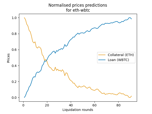
(a)

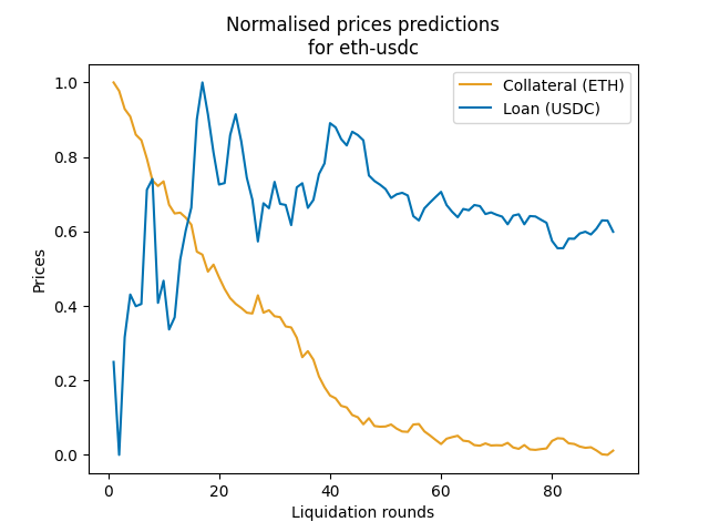
(b)

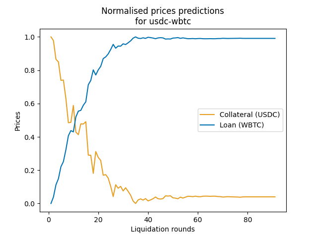
(c)

Figure 10: Prices predictions produced, for each scenario in Table 3, by GBMs instantiated with the parameters in Figure 5.

We have used the MultiVeStA statistical analyzer to examine the prices predictions generated by the GBM in each of the scenarios explained in Section 3.2.2. The details are provided in the appendix ( Figure 10), and show the normalised trend of the price scenarios, discussed in Section 3.2.2. The figures in the appendix show that the expected behaviour, expressed in Table 3 is obtained in all the considered scenarios. Additionally, in Figures 10(a) and 10(c) prices predictions are strongly correlated as it is expected. In fact, the GBMs pairs were instantiated as negatively correlated processes accordingly to [20], Section 14.5. Contrarily, Figure 10(b) shows less correlated prices predictions. This is probably due to the fact that the computation was bounded to execute maximum $5,010$ simulations. In fact, from experimental evidence, the approximation seem to converge at a very slow speed.

4 Statistical Analysis of Liquidation Scenarios

We have experimented with the LP model simulator described in Section 3 in order to answer the question: given a specific scenario, what is the impact of the pair of LP parameters $C_{\mathrm{min}}$ and $r_{\mathrm{liq}}$?

We have considered scenarios generated by four factors. First, the liquidator logic defined in Section 3.1, determines immediate and quick liquidations, causing a significant financial loss to the liquidated party. Secondly, the agent to be liquidated is selected so to maximise the value of seized collateral, which is the most beneficial and rational option for liquidators. Thirdly, liquidators are assumed to hold an unbounded amount of resources, which allows them to repeat liquidations as long as there exists an undercollaterized agent. Finally, cryptoasset prices evolve following a trend aimed at causing borrowers to suddenly become undercollaterized.

Figure 6: Distribution of collateralization in initial configurations.

We recall that the effect of the pair $C_{\mathrm{min}}$ and $r_{\mathrm{liq}}$ we are looking for is one that minimises the number of undercollaterized borrowers. We have explored the space of choices for the pair by executing MultiVeStA experiments for all $C_{\mathrm{min}}$ ranging, with step $0.1$, from $1.2$ to $1.5$ and $r_{\mathrm{liq}}$ ranging from $1.1$ to $C_{\mathrm{min}}-0.1$. These ranges were selected based on the values typically assigned to these parameters in the actual implementations: $C_{\mathrm{min}}=1.5$ and $r_{\mathrm{liq}}=1.1$ [6].

On these premises, we first illustrate the LP model initial configurations used for the subsequent experimentation. Next, we present the results of the performed experiments.

4.0.1 Initial configurations

The initial configurations were designed to test the resistance of different borrowers’ collateralization to becoming unrecoverable, when subject to repeated liquidations. Since the intention is to observe the model behaviour under three price models (Section 3.2.2), three different initial configurations are produced, each having a different price for collateral and loan assets. All the configurations share the same amount and types of agents. Specifically, a generic initial configuration comprises ten borrowers having collateralization ranging from 1.0 to 2.0, with step 0.1. This is depicted in Figure 6, where $b_{i}$ represents the generic borrower $\mathit{B_{i}}$’s collateralization ($C_{\Gamma^{i}}(\mathit{B_{i}})$), for $\Gamma^{i}$ initial configuration. Additionally, an arbitrary number of liquidators (three) are added to each configuration.

4.0.2 Experimental results

The results discussed here were obtained by performing MultiVeStA experiments of the LP simulator. Specifically, the inputs to the tool are: the LP simulator discussed in Section 3, a MultiQuaTEx property to express the desired measure to be estimated (the expected collateralization value at each liquidation round for each borrower), and a pair of statistical parameters defining the confidence interval (CI) of interest: the maximum confidence interval width $\delta$ and the confidence level $\alpha=0.05$ which provides 95% statistical confidence that the estimated value is in the confidence interval. For each property, MultiVeStA will generate enough simulation to meet the required CI.

Figure 7: Per-borrower collateralization ($\mathrm{b_{1}\ to\ b_{10}}$) in the ETH-WBTC prices scenario, for varying liquidation rounds and CMin-Rliq choices.

Figure 7 shows the per-borrower collateralization for varying liquidation rounds and choices of $C_{\mathrm{min}}$ and $r_{\mathrm{liq}}$ in the eth-wbtc prices scenario, with a fixed $r_{\mathrm{liq}}=1.1$. In this scenario, one can see that undercollaterized agents have a very different behaviour than overcollaterized ones. Specifically, the undercollaterized agents undergo very serious liquidations, which often lead them to unrecoverability, as their collateralization converges to a constant below $C_{\mathrm{min}}$. Contrarily, overcollaterized agents do not incur in severe financial losses.

Additionally, our experiments (presented in detail in the Appendix, Figures 11(a), 11(b) and 11(c)) show that the $C_{\mathrm{min}}$ and $r_{\mathrm{liq}}$ having the least negative effects on undercollaterized balances is $C_{\mathrm{min}}=1.5$, $r_{\mathrm{liq}}=1.1$. This is also quantitatively confirmed by the numbers in Figure 8. Intuitively, this is a consequence of the fact that when $C_{\mathrm{min}}=1.5$ and $r_{\mathrm{liq}}=1.1$ the collateralization of each agent $b_{1}$ to $b_{5}$ is higher on average than for any other $C_{\mathrm{min}}$ and $r_{\mathrm{liq}}$ pairs. As a result, the number of unrecoverable loans, the ones held by agents whose collateralization is below $1$, is minimised.

Price scenario	(CMin-Rliq)
	(1.5-1.1)	(1.4-1.1)	(1.3-1.1)
ETH-WBTC	0.7115	0.6518	0.6137
ETH-USDC	0.7106	0.6583	0.6231
USDC-WBTC	0.8381	0.7739	0.7299

Figure 8: Minimum average $C_{\Gamma}(\mathit{B_{1}})$

Finally, our experiments (presented in detail in the Appendix, Figures 12(a), 12(b) and 12(c)) show that overcollaterized borrowers could still incur in liquidations, in case the prices abruptly change as in the prices scenario ETH-WBTC. Differently, in the other scenarios, employing the stable coin USDC, overcollaterized agents are, on average, rarely liquidated.

5 Related Works

Verification of DeFi applications is a fairly recent research area where several techniques have been applied. We focus our discussion on works devoted to formal modelling and reasoning of DeFi applications, which typically follow two parallel directions: verification of the model properties [9, 5, 2, 32], and statistical analysis of the model variables [4, 14, 22, 13, 19].

The work in [9] is one of the first addressing formal verification of smart contract properties. Their study combines a game-theoretic approach with probabilistic model checking, ultimately validating their results with the model checker PRISM [23]. Another example of research in this direction is Tolmach et al. [32] which developed the first multi-pools model and verified invariant properties initially formulated by [8]. Finally, [2] proposed a very relevant study on smart contracts, by modelling not only the contracts and the agents’ behaviour but also the underlying blockchain using the BIP framework [7] and statistical model checking (as we do). The work in  [2] employs statistical methods too. However, in their case, statistics is useful to estimate unknown variables of the analysed model, hence deriving desirable properties. The quantitative variables estimation is also achieved by performing Monte-Carlo simulations, with a more closely look at the behaviours displayed by agents [14]. In fact, most of this research in this line [22, 13, 4] bases its results on Agent-Based Simulations, which is employed to stress test the actual smart contracts implementations being executed on a “custom-built Ethereum virtual machine that is written in C++” [22]. This research direction, although suggesting promising results, is not ultimately supported by strong statistical guarantees, since the number of Monte Carlo simulations performed to run their analyses is arbitrarily chosen and not backed by a formal justification [22, 19]. Nonetheless, a work relevant to ours is the analysis conducted in [22] on the Compound protocol scalability in face of high stock market prices volatility. Similarly to our work, their analysis models the prices by the use of the GBM. However, their data collection and analysis methodologies are very different. In fact, they do not sample entire historical periods as illustrated in Section 3.2 for estimating prices volatility. Contrarily, they simply evaluate the minimum and maximum volatility values ever observed and instantiate the GBM for different prices volatilities so to simulate several market environments. Finally, the prices model in Section 3.2 has been mostly inspired by [19]. Similarly to [22], they stress-test an LP model, not a specific implementation, by using the same price model explained in Section 3.2. Nonetheless, a remarkable difference is that they instantiate the predictions of the collateral and loan assets pairs with three different correlation parameters. We assume instead predictions of prices pairs to be strongly negatively correlated ($\rho=-1$), in order to simulate the worst-case scenario. Additionally, we reproduced [19]’s environment by using historical data of three different real cryptoassets on the market.

6 Conclusions

We have presented a tool for the analysis of lending pools, an archetypal DeFi application. Overall the tool consists of (i) an accurate LP simulator based on the model of [6] which can support both the study of vulnerabilities and attacks of LPs; (ii) a model checker capable of doing simple reachability analysis and verifying whether LTL properties hold of specific configurations; and (iii) a tool for statistical analysis backed by the statistical model checker MultiVeStA. In this paper, we have focused on (iii) and we have shown how to use it to optimize the LP parameters under specific scenarios. Details on (i) and (ii) as well as further examples, including reproduction of price oracle attacks using reachability analysis and LTL model checking are available in [25].

Future research supported by the developed tool could include the formalization of further attacks and properties of the model. Specifically, one could study resistance to illiquidity, as suggested by [22], or the behaviour of multi-pools configurations, each offering different market opportunities to agents, as proposed by [35] and partially developed in [32].

Acknowledgements

Massimo Bartoletti is partially supported by Conv. Fondazione di Sardegna & Atenei Sardi project F75F21001220007 ASTRID. James Hsin-yu Chiang is supported by the PhD School of DTU Compute. Alberto Lluch Lafuente is partially supported by the EU H2020-SU-ICT-03-2018 Project No. 830929 CyberSec4Europe (cybersec4europe.eu). Andrea Vandin is partially supported by the DFF project REDUCTO 9040-00224B.

Appendix 0.A Figures

(a) 13/01/2018-14/04/2018

(b) 01/01/2020-01/04/2020

(c) 24/11/2020-23/02/2021

Figure 9: Trimester closing prices, collected from CoinGecko APIs

(a) Scenario: eth-wbtc.

(b) Scenario: eth-usdc.

(c) Scenario: usdc-wbtc.

Figure 11: Per-borrower collateralization ($\mathrm{b_{1}}$ to $\mathrm{b_{5}}$) in the three prices scenarios, for varying CMin-rliq choices.

(a) Scenario: eth-wbtc.

(b) Scenario: eth-usdc.

(c) Scenario: usdc-wbtc.

Figure 12: Per-borrower collateralization ($\mathrm{b_{3}}$ to $\mathrm{b_{7}}$) in the three prices scenarios, for varying CMin-rliq choices.

References

- [1] Aave, S.: Aave markets - webpage. https://aave.com/ (2021)
- [2] Abdellatif, T., Brousmiche, K.L.: Formal verification of smart contracts based on users and blockchain behaviors models. In: 2018 9th IFIP International Conference on New Technologies, Mobility and Security (NTMS). pp. 1–5. IEEE (2018)
- [3] Agha, G., Palmskog, K.: A survey of statistical model checking. ACM Transactions on Modeling and Computer Simulation (TOMACS) 28(1), 1–39 (2018)
- [4] Angeris, G., Kao, H.T., Chiang, R., Noyes, C., Chitra, T.: An analysis of Uniswap markets. Cryptoeconomic Systems (1) (2021). https://doi.org/10.21428/58320208.c9738e64
- [5] Bai, X., Cheng, Z., Duan, Z., Hu, K.: Formal modeling and verification of smart contracts. In: Proceedings of the 2018 7th International Conference on Software and Computer Applications. pp. 322–326 (2018)
- [6] Bartoletti, M., Chiang, J.H., Lluch-Lafuente, A.: SoK: Lending pools in decentralized finance. In: Financial Cryptography Workshops. LNCS, vol. 12676, pp. 553–578. Springer (2021). https://doi.org/10.1007/978-3-662-63958-0_40, the Lending Pools model used in this paper is taken from a preliminary version of the paper, published as arXiv preprint 2012.13230.
- [7] Basu, A., Bensalem, B., Bozga, M., Combaz, J., Jaber, M., Nguyen, T.H., Sifakis, J.: Rigorous component-based system design using the BIP framework. IEEE software 28(3), 41–48 (2011)
- [8] Bernardi, T., Dor, N., Fedotov, A., Grossman, S., Immerman, N., Jackson, D., Nutz, A., Oppenheim, L., Pistiner, O., Rinetzky, N., et al.: Wip: Finding bugs automatically in smart contracts with parameterized invariants. https://groups.csail.mit.edu/sdg/pubs/2020/sbc2020.pdf (2020)
- [9] Bigi, G., Bracciali, A., Meacci, G., Tuosto, E.: Validation of decentralised smart contracts through game theory and formal methods. In: Programming Languages with Applications to Biology and Security, pp. 142–161. Springer (2015)
- [10] Boado, E.: Aave whitepaper. https://github.com/aave/protocol-v2/blob/master/aave-v2-whitepaper.pdf (2020), accessed on 26.02.2021 - commit aeded1520c667e59a564cf69f33a6e489b2fe489
- [11] Boado, E., Aave, S.: Aave protocol maximum liquidate threshold. https://github.com/aave/aave-protocol/blob/1ff8418eb5c73ce233ac44bfb7541d07828b273f/contracts/lendingpool/LendingPoolLiquidationManager.sol#L181 (2021)
- [12] Buterin, V.: Ethereum whitepaper. https://ethereum.org/en/whitepaper/ (2013), accessed on 24.02.2021
- [13] Chitra, T., Evans, A.: Why stake when you can borrow? CoRR abs/2006.11156 (2020), https://arxiv.org/abs/2006.11156
- [14] Chitra, T., Quaintance, M., Haber, S., Martino, W.: Agent-based simulations of blockchain protocols illustrated via Kadena’s chainweb. In: 2019 IEEE European Symposium on Security and Privacy Workshops (EuroS&PW). pp. 386–395. IEEE (2019)
- [15] Clavel, M., Durán, F., Eker, S., Escobar, S., Lincoln, P., Martı-Oliet, N., Meseguer, J., Rubio, R., Talcott, C.: Maude manual (version 3.0). Tech. rep., Technical report, SRI International Computer Science Laboratory (2020)
- [16] Compound Labs, I.: Compound markets - webpage. https://compound.finance/markets (2021)
- [17] Dmouj, A.: Stock price modelling: Theory and practice. Masters Degree Thesis, Vrije Universiteit (2006)
- [18] Entriken, W.: Introduction to smart contracts. https://ethereum.org/en/developers/docs/smart-contracts/ (2020), accessed on 27.02.2021
- [19] Gudgeon, L., Perez, D., Harz, D., Livshits, B., Gervais, A.: The decentralized financial crisis. In: 2020 Crypto Valley Conference on Blockchain Technology (CVCBT). pp. 1–15. IEEE (2020)
- [20] Hull, J.C.: Options futures and other derivatives. Pearson Education India (2003)
- [21] Jeffrey, G.: Compound price oracle attack. https://news.bitcoin.com/100-million-liquidated-on-defi-protocol-compound-following-oracle-exploit/ (2020)
- [22] Kao, H.T., Chitra, T., Chiang, R., Morrow, J.: An analysis of the market risk to participants in the Compound protocol. In: Third International Symposium on Foundations and Applications of Blockchains (2020)
- [23] Kwiatkowska, M., Norman, G., Parker, D.: PRISM 4.0: Verification of probabilistic real-time systems. In: Gopalakrishnan, G., Qadeer, S. (eds.) Proc. 23rd International Conference on Computer Aided Verification (CAV’11). LNCS, vol. 6806, pp. 585–591. Springer (2011)
- [24] Leshner, R., Hayes, G.: Compound: The money market protocol. https://compound.finance/documents/Compound.Whitepaper.v04.pdf (2019)
- [25] Mirelli, M.: A formal verification tool for Lending Pools. Master’s thesis, Aalto University. School of Science (2021), http://urn.fi/URN:NBN:fi:aalto-202108298504
- [26] Mirelli, M.: A Maude simulator for Lending Pools. https://github.com/MMirelli/maude-lp (2021), accessed on 22.06.2022 - commit 2dae39b035938f5f9791040c53121fb473b4b7dd
- [27] Perez, D., Werner, S.M., Xu, J., Livshits, B.: Liquidations: DeFi on a knife-edge. In: Financial Cryptography and Data Security. LNCS, vol. 12675, pp. 457–476. Springer (2021). https://doi.org/10.1007/978-3-662-64331-0_24
- [28] Peterins, E., Flatow, J., Hayes, G., Wolff, M., Greenberg, A.: Compound protocol maximum liquidate threshold. https://github.com/compound-finance/compound-protocol/blob/4e99ea3a64ab4f1bdf9c07c7a1bf325db09ab809/scenario/src/Event/ComptrollerEvent.ts#L170 (2021)
- [29] Pulse: Defi pulse - webpage. https://defipulse.com (2021), accessed on 07.06.2021
- [30] Qin, K., Zhou, L., Livshits, B., Gervais, A.: Attacking the DeFi ecosystem with flash loans for fun and profit. In: Financial Cryptography. LNCS, vol. 12674, pp. 3–32. Springer (2021). https://doi.org/10.1007/978-3-662-64322-8_1
- [31] Sebastio, S., Vandin, A.: Multivesta: Statistical model checking for discrete event simulators. Tech. rep., IMT Institute for Advanced Studies Lucca (2013)
- [32] Tolmach, P., Li, Y., Lin, S.W., Liu, Y.: Formal analysis of composable defi protocols. arXiv preprint arXiv:2103.00540 (2021)
- [33] Vandin, A., Giachini, D., Lamperti, F., Chiaromonte, F.: Automated and distributed statistical analysis of economic agent-based models. arXiv preprint arXiv:2102.05405 (2021)
- [34] Wackerow, P., Rhechler: Decentralized finance (defi) - webpage. https://ethereum.org/en/defi/ (2021), accessed on 02.06.2021
- [35] Werner, S.M., Perez, D., Gudgeon, L., Klages-Mundt, A., Harz, D., Knottenbelt, W.J.: SoK: Decentralized Finance (DeFi). CoRR abs/2101.08778 (2021), https://arxiv.org/abs/2101.08778
- [36] Zhou, L., Qin, K., Cully, A., Livshits, B., Gervais, A.: On the just-in-time discovery of profit-generating transactions in DeFi protocols. In: IEEE Symposium on Security and Privacy. pp. 919–936. IEEE (2021). https://doi.org/10.1109/SP40001.2021.00113