Decentralized Training of Foundation Models in Heterogeneous Environments

Abstract

Training foundation models, such as GPT-3 and PaLM, can be extremely expensive, often involving tens of thousands of GPUs running continuously for months. These models are typically trained in specialized clusters featuring fast, homogeneous interconnects and using carefully designed software systems that support both data parallelism and model/pipeline parallelism. Such dedicated clusters can be costly and difficult to obtain. Can we instead leverage the much greater amount of decentralized, heterogeneous, and lower-bandwidth interconnected compute? Previous works examining the heterogeneous, decentralized setting focus on relatively small models that can be trained in a purely data parallel manner. State-of-the-art schemes for model parallel foundation model training, such as Megatron and Deepspeed, only consider the homogeneous data center setting. In this paper, we present the first study of training large foundation models with model parallelism in a decentralized regime over a heterogeneous network. Our key technical contribution is a scheduling algorithm that allocates different computational “tasklets” in the training of foundation models to a group of decentralized GPU devices connected by a slow heterogeneous network. We provide a formal cost model and further propose an efficient evolutionary algorithm to find the optimal allocation strategy. We conduct extensive experiments that represent different scenarios for learning over geo-distributed devices simulated using real-world network measurements. In the most extreme case, across 8 different cities spanning 3 continents, our approach is 4.8$\times$ faster than prior state-of-the-art training systems.

1 Introduction

Recent years have witnessed the rapid development of deep learning models, particularly foundation models (FMs) Bommasani et al. (2021) such as GPT-3 Brown et al. (2020) and PaLM Chowdhery et al. (2022). Along with these rapid advancements, however, comes computational challenges in training these models: the training of these FMs can be very expensive — a single GPT3-175B training run takes 3.6K Petaflops-days Brown et al. (2020)— this amounts to $4M on today’s AWS on demand instances, even assuming 50% device utilization (V100 GPUs peak at 125 TeraFLOPS)! Even the smaller scale language models, e.g., GPT3-1.3B (1.3 billion parameters), on which this paper evaluates, require 64 Tesla V100 GPUs to run for one week, costing $32K on AWS. As a result, speeding up training and decreasing the cost of FMs have been active research areas. Due to their vast number of model parameters, state-of-the-art systems (e.g., MegatronShoeybi et al. (2019), DeepspeedRasley et al. (2020), FairscaleBaines et al. (2021)) leverage multiple forms of parallelism Shoeybi et al. (2019); Xu et al. (2021); Zheng et al. (2022); Li et al. (2021); Rajbhandari et al. (2020); Ren et al. (2021). However, their design is only tailored to fast, homogeneous data center networks.

Figure 1: Given ① a set of computation tasklets involved in training foundation models (corresponding to different micro-batches and layers), and ② a heterogeneous network between devices, the goal is to find the optimal ③ allocation of tasklets to devices.

On the other hand, decentralization is a natural and promising direction. Jon Peddie Research reports that the PC and AIB GPU market shipped 101 million units in Q4 2021 alone gpu . Furthermore, many of these GPUs are underutilized. Leveraging this fact, volunteer computing projects such as Folding@Home Shirts and Pande (2000) have sourced upwards of 40K Nvidia and AMD GPUs continuously fol (2022). Moreover, the incremental electricity and HVAC costs of running a V100 GPU for a volunteer are 50–100$\times$ lower than the spot prices for an equivalent device on AWS eco . If we could make use of these devices in a decentralized open-volunteering paradigm for foundation model training, this would be a revolutionary alternative to the expensive solutions offered by data centers.

This vision inspired many recent efforts in decentralized learning, including both those that are theoretical and algorithmic Lian et al. (2017); Koloskova et al. (2019, 2020), as well as recent prototypes such as Learning@Home Ryabinin and Gusev (2020) and DeDLOC Diskin et al. (2021). However, efforts to-date in decentralized training either focus solely on data parallelism Lian et al. (2017); Koloskova et al. (2019, 2020); Diskin et al. (2021), which alone is insufficient for FMs whose parameters exceed the capacity of a single device, or orient around alternative architectures, e.g., mixture of experts Ryabinin and Gusev (2020). These alternative architectures provide promising directions for decentralized learning, however, they are currently only trained and evaluated on smaller datasets and at a smaller computational scale (e.g., MNIST and WikiText-2 in Ryabinin and Gusev (2020)) than their state-of-the-art counterparts, e.g., GLaM Du et al. (2021). In this paper, we focus on a standard GPT-style architecture, without considering any changes that might alter the model architecture or the convergence behaviour during training.

To fulfill the potential of decentralization for the training of FMs, we need to be able to (1) take advantage of computational devices connected via heterogeneous networks with limited bandwidth and significant latency, and (2) support forms of parallelism beyond pure data parallelism. In this paper, we tackle one fundamental aspect of this goal — how can we assign different computational “tasklets”, corresponding to a micro-batch and a subset of layers, to a collection of geo-distributed devices connected via heterogeneous, slow networks? This is not an easy task — even for fast and homogeneous data center networks, such assignments are still an open ongoing research challenge Narayanan et al. (2019); Tarnawski et al. (2020, 2021); Fan et al. (2021); Park et al. (2020). For the heterogeneous setting, it becomes even more challenging as the size of the search space increases dramatically. In the homogeneous setting, the homogeneity of the edges in the communication graph reduces the search space into many equivalent classes representing allocation strategies with the same communication costs, enabling efficient polynomial runtime algorithms Tarnawski et al. (2020, 2021); Narayanan et al. (2019); Fan et al. (2021); Park et al. (2020); however, in the heterogeneous setting, one has to consider potentially exponentially many more distinct allocation strategies — as we will see later, because of the heterogeneity of the communication matrix, even the sub-problem of finding the best pipeline parallelism strategy equates to a hard open loop travelling salesman problem Papadimitriou (1977).

In this paper, we focus on this challenging scheduling problem of decentralized training of FMs over slow, heterogeneous networks, and make the following contributions:

• We study the problem of allocating distributed training jobs over a group of decentralized GPU devices connected via a slow heterogeneous network. More specifically:

  • To capture the complex communication cost for training FMs, we propose a natural, but novel, formulation involving decomposing the cost model into two levels: the first level is a balanced graph partitioning problem corresponding to the communication cost of data parallelism, whereas the second level is a joint graph matching and traveling salesman problem corresponding to the communication cost of pipeline parallelism.

  • We propose a novel scheduling algorithm to search for the optimal allocation strategy given our cost model. Developing a direct solution to this optimization problem is hard; thus, we propose an efficient evolutionary algorithm based on a collection of novel heuristics, going beyond the traditional heuristics used in standard graph partitioning methods Kang and Moon (2000).

• We carefully designed and implemented a collection of system optimizations to hide communication within the computation to further reduce the impact of slow connections.

• We conduct extensive experiments that represent different scenarios of collaborative decentralized learning, simulated by using network measurements from different geographical regions of AWS. In the worldwide setting with 64 GPUs across 8 regions (Oregon, Virginia, Ohio, Tokyo, Seoul, London, Frankfurt, Ireland), we show that our system is 3.8-4.8$\times$ faster, in end-to-end runtime, than the state-of-the-art systems, for training GPT3-1.3B, without any difference in what is computed or convergence dynamics. In addition, we also provide careful ablation studies to show the individual effectiveness of the scheduler and system optimizations.

• We shed light on the potential of decentralized learning — our prototype in the global heterogeneous setting is only 1.7-3.5$\times$ slower than Megatron/Deepspeed in data centers even though its network can be 100$\times$ slower. We hope this paper can inspire future explorations of decentralized learning for FMs, over geo-distributed servers, desktops, laptops, or even mobile devices.

Limitations and Moving Forward. In this paper, we tackle one foundational aspect of decentralized learning but leave as future work many problems that are important for a practical system. We assume that communication between devices is relatively stable for a reasonable amount of time and that all devices are always online without failure or eviction. Note that we also do not train a full system to full convergence, instead running partial training to confirm intermediate result equivalence across regimes. Scheduling over a dynamic, heterogeneous environment and providing fault tolerance, potentially with checkpointing, while training to convergence are directions for future exploration.

2 Decentralized Training of Foundation Models: Problem Formulation

We first introduce concepts, technical terms, and the procedure of decentralized training. Then we formally define the scheduling problem this paper tackles.

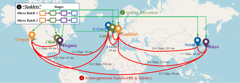
Decentralized setting. We assume a group of devices (GPUs) participating in collaborative training of a foundation model. Each pair of devices has a connection with potentially different delay and bandwidth. These devices can be geo-distributed, as illustrated in Figure 1, with vastly different pairwise communication bandwidth and latency. In decentralized training, all layers of a model are split into multiple stages, where each device handles a consecutive sequence of layers, e.g., several transformer blocks Vaswani et al. (2017). In addition, since the input for foundation model pre-training is huge, e.g., a few millions of tokens, it is also split into multiple micro-batches that can be handled in parallel.

Problem definition. We define tasklets as a collection of computational tasks in foundation model training — Tasklet $t_{i,j}$ is the forward and backward computation for a stage $j$ with a micro-batch $i$ of training data in a training iteration. We aim to design an effective scheduler to assign each tasklet to a particular device so that the training throughput is maximized in decentralized training.

Parallelism. The above setting involves two forms of parallelism, pipeline and data. In pipeline parallelism, the compute in multiple stages is parallelized — each device handles activation or gradient computation for different micro-batches in parallel and the results can be communicated or passed to subsequent stages. Data parallelism means that devices compute the gradient for different micro-batches independently, but need to synchronize these gradients through communication. In a decentralized environment, the training procedure is communication-bounded. The scheduling problem is to accelerate the communication procedure by allocating tasklets that require high communication volumes between them to devices with faster connections.

Formalization of the scheduling problem. Formally, our scheduling problem is as follows.

• Let $\mathbf{D}=\{d_{1}\ldots d_{N}\}$ be a set of $N$ devices; $\mathbf{A}\in\mathbb{R}_{+}^{N\times N}$ and $\mathbf{B}\in\mathbb{R}_{+}^{N\times N}$ be the communication matrix between these devices describing the delay and bandwidth respectively, where the delay and bandwidth between device $d$ and $d^{\prime}$ is $\alpha_{d,d^{\prime}}$ and $\beta_{d,d^{\prime}}$.

• Given the communication matrix $\mathbf{A}$ and $\mathbf{B}$, we construct a communication graph $\mathbf{G}$ (Figure 2(a)) — each device corresponds to a node in $\mathbf{G}$ and each edge between $d$ and $d^{\prime}$ is labeled with the average latency and bandwidth between $d$ and $d^{\prime}$: $((\alpha_{d,d^{\prime}}+\alpha_{d^{\prime},d})/2,(\beta_{d,d^{\prime}}+\beta_{d^{\prime},d})/2)$. Even though $\mathbf{A}$ and $\mathbf{B}$ are asymmetric (i.e., upload and download speeds might be different), the communication graph $\mathbf{G}$ is symmetric because in our workloads all communications between two devices happen to involve the same amount of upload and download.

• The number of stages that a micro-batch needs to go through is $D_{\textsc{pp}}$ (noted as pipeline parallel degree); the number of batch partition that needs to run model gradient synchronization is $D_{\textsc{dp}}$ (noted as data parallel degree); we have $D_{\textsc{dp}}\times D_{\textsc{pp}}=N$, i.e., the total number of devices.

• $c_{\textsc{pp}}$ (resp. $c_{\textsc{dp}}$) represent the number of bytes of activations for a micro-batch (resp. parameters/gradients for a stage) communicated in pipeline parallelism (resp. data parallelism).

• We denote a training tasklet as $t_{i,j}$, where $i\in\{1,...,D_{\textsc{dp}}\}$ and $j\in\{1,...,D_{\textsc{pp}}\}$, each of which corresponds to one specific micro-batch $i$ and pipeline stage $j$.

• An assignment strategy $\sigma\in\mathbf{D}^{D_{\text{DP}}\times D_{\text{PP}}}$ assigns, for each tasklet $t_{i,j}$, a device $\sigma_{i,j}\in\mathbf{D}$, which means that device $\sigma_{i,j}$ runs the training tasklet $t_{i,j}$. A valid assignment needs to be unique, i.e., $\forall(i,j)\neq(i^{\prime},j^{\prime})$: $\sigma_{i,j}\neq\sigma_{i^{\prime},j^{\prime}}$. We use $\Sigma$ to denote the set of all valid assignments.

• An optimal assignment strategy is an assignment $\sigma$ that minimizes the communication cost

  $$\sigma^{*}=\arg\min_{\sigma\in\Sigma}\textsc{Comm-Cost}\left(\sigma\right)$$

Challenges and Goals. Our goal is to find the optimal assignment strategy, which involves two challenges: (1) How to effectively model the communication cost $\textsc{Comm-Cost}(\sigma)$ for a given assignment $\sigma$ under a heterogeneous network environment? and (2) How to effectively search for the optimal assignment strategy that minimizes such a cost? We tackle these two questions in Section 3.

3 Scheduling in Heterogeneous Environments

Scheduling in the heterogeneous setting is a challenging task, as the size of the search space increases dramatically compared to that of the homogeneous case. In the homogeneous data-center case, the network delay can be usually ignored (e.g., $\mathbf{A}=\mathbf{0}$) and the bandwidth $\mathbf{B}$ are assumed to be formed by just a few constants — e.g., the communication bandwidths between different machines on the same rack are assumed to be same Tarnawski et al. (2020, 2021); Narayanan et al. (2019, 2019); Park et al. (2020). This significantly constrains the search space — one can ignore the influence of communication given uniform connections Tarnawski et al. (2020, 2021); Narayanan et al. (2019), or organize the device with a hierarchical structure Narayanan et al. (2019); Park et al. (2020), making the scheduling problem solvable in polynomial time in terms of the number of machines.

In contrast, in the fully heterogeneous scenario the communication matrix $\mathbf{A}$ and $\mathbf{B}$ consists of distinct values, which can make the search space grows exponentially. In this section, we describe our scheduler that searches for an optimal strategy in the complex search space.

Figure 2: (a) Communication graph $\mathbf{G}$; and (b, c, d, e) an illustration of the cost model given $\mathbf{G}$.

3.1 Overview of the scheduler

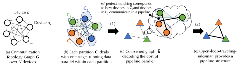
We carefully design a bi-level scheduling algorithm based on extended balanced graph partition problem (see Figure 2), and solve this problem by an evolutionary algorithm with a carefully designed local search strategy. Given an assignment strategy $\sigma=\{\sigma_{i,j}\}$ for all tasklets $\{t_{i,j}\}$, we first model its communication cost. During the training of FMs, the communication costs come from two different sources: (1) Data parallel: All devices that are assigned with the tasklets dealing with the same stage $j$ (handling the same layers) of different micro-batches need to communicate within themselves to exchange gradients of these layers. For layer $j$, we call these devices its data parallel group: $\mathbf{C}_{j}=\{\sigma_{i,j}~{}|~{}\forall i\in\left[D_{\textsc{dp}}\right]\}$. We can implement the communication using different primitives, e.g., AllReduce Sergeev and Del Balso (2018), ScatterGatter Jiang et al. (2020), or other decentralized average protocols Lian et al. (2017). (2) Pipeline parallel: All devices that are assigned with the tasklets dealing with the same micro-batch $i$ of different stages need to form a pipeline, communicating within themselves to exchange activations and backward gradients. For micro-batch $i$, these devices are $\mathbf{P}_{i}=\{\sigma_{i,j}~{}|~{}\forall j\in[D_{\textsc{pp}}]\}$. Because these devices need to form a linear pipeline, any permutation over $\mathbf{P}_{i}$ corresponds to one strategy of how these machines can conduct pipeline parallelism within them.

Scheduling Problem. The goal of our scheduler is to minimize both costs. One design decision that we made is to decompose this complex optimization problem into two levels. At the first level, we consider the best way of forming $\mathbf{C}_{j}$’s, incurring data parallel communication costs within them. At the second level, we consider the cost of pipeline parallelism given an layout from the first level:

$$\min_{\mathbf{C}_{1}...\mathbf{C}_{D_{\textsc{pp}}}}\textsc{Comm-Cost}\left(\mathbf{C}_{1}...\mathbf{C}_{D_{\textsc{pp}}}\right):= \textsc{DataP-Cost}(\mathbf{C}_{1}...\mathbf{C}_{D_{\textsc{pp}}})$$ (1)

$$+\textsc{PipelineP-Cost}(\mathbf{C}_{1}...\mathbf{C}_{D_{\textsc{pp}}})$$

$$s.t.\quad|\mathbf{C}_{1}|=....=|\mathbf{C}_{D_{\textsc{pp}}}|=D_{\textsc{dp}}, \forall j,j^{\prime}:\mathbf{C}_{j}\cap\mathbf{C}_{j^{\prime}}=\emptyset,\mathbf{C}_{1}\cup...\cup\mathbf{C}_{D_{\textsc{pp}}}=\mathbf{D}$$

where computing $\textsc{PipelineP-Cost}(\mathbf{C}_{1}...\mathbf{C}_{D_{\textsc{pp}}})$ involves finding the optimal pipeline structure.

In Section 3.2 and Section 3.3, we provide details on $\textsc{Comm-Cost}\left(\mathbf{C}_{1}...\mathbf{C}_{D_{\textsc{pp}}}\right)$. Notice that this modified objective makes our problem different from the textbook graph partition problem; thus, we need a carefully designed evolutionary algorithm for finding such a solution introduced in Section 3.4.

3.2 Modelling data parallel communication cost

Given the communication graph $\mathbf{G}$ forming data parallel groups $\mathbf{C}_{1}...\mathbf{C}_{D_{\textsc{pp}}}$ corresponds to a partition of $\mathbf{G}$— In Figure 2(b), different colors correspond to devices in the same $\mathbf{C}_{j}$. The data parallel cost within $\mathbf{C}_{j}$ only relies on all communication channels (edges in the communication graph) connecting devices in $\mathbf{C}_{j}$. If we assume a colocated sharded parameter server Jiang et al. (2020) implementation for communicating within each $\mathbf{C}_{j}$, and recall that $c_{\textsc{dp}}$ represents the total amount of data (in bytes) that needs to be exchanged during gradient aggregation — each device in $\mathbf{C}_{j}$ needs to manage ${c_{\textsc{dp}}}/{D_{\textsc{dp}}}$ bytes of parameter shard. Once the gradient is ready, each device needs to send each of its local shards to the corresponding device; next, each device can aggregate the gradients it receives from all other devices in $\mathbf{C}_{j}$; and finally, each device will send the aggregated gradient shard to all other devices. Therefore, we can model the data parallel cost for $\mathbf{C}_{j}$ as follows:

$$\textsc{DataP-Cost}(\mathbf{C}_{j})=\max_{d\in\mathbf{C}_{j}}\sum_{d^{\prime}\in\mathbf{C}_{j}-\{d\}}2\cdot\left(\alpha_{d,d^{\prime}}+\frac{c_{\text{dp}}}{D_{\textsc{dp}}{\beta}_{d,d^{\prime}}}\right).$$ (2)

Here, the total cost is bounded by the slowest device ($\max_{d\in\mathbf{C}_{j}}$), which needs to exchange data with all other machines ($\sum_{d^{\prime}\in\mathbf{C}_{j}-\{d\}}$). Because the communication of these different data parallel groups $\mathbf{C}_{1}...\mathbf{C}_{D_{\textsc{pp}}}$ can be conducted in parallel and we are only bounded by the slowest data parallel group. This allows us to model the total communication cost for data parallelism as:

$$\textsc{DataP-Cost}(\mathbf{C}_{1}...\mathbf{C}_{D_{\textsc{pp}}})=\max_{j\in\left[D_{\textsc{pp}}\right]}\textsc{DataP-Cost}(\mathbf{C}_{j})$$

3.3 Modeling pipeline parallel communication cost

Given $\mathbf{C}_{1}...\mathbf{C}_{D_{\textsc{pp}}}$, to model the communication cost of pipeline parallelism, we need to consider two factors: (1) each permutation $\pi$ of {$\mathbf{C}_{1}...\mathbf{C}_{D_{\textsc{pp}}}$} corresponds to a specific pipeline strategy — devices in $\mathbf{C}_{\pi_{j}}$ and devices in $\mathbf{C}_{\pi_{j+1}}$ communicates to exchange activations (during forward pass) and gradients on activations (during backward pass); and (2) devices in $\mathbf{C}_{\pi_{j}}$ and devices in $\mathbf{C}_{\pi_{j+1}}$ need to be “matched” — only devices that are dealing with the same micro-batch needs to communicate. This makes modeling the cost of pipeline parallel communication more complex.

To model the cost of pipeline parallel communication, we first consider the best possible way that devices in $\mathbf{C}_{j}$ and $\mathbf{C}_{j^{\prime}}$ can be matched. We do this by creating a coarsened communication graph (Figure 2(c)). A coarsened communication graph ${\mathbf{\widehat{G}}}_{\mathbf{C}_{1}...\mathbf{C}_{D_{\textsc{pp}}}}$ is a fully connected graph, and each partition $\mathbf{C}_{j}$ in the original communication graph $\mathbf{G}$ corresponds to a node in ${\mathbf{\widehat{G}}}_{\mathbf{C}_{1}...\mathbf{C}_{D_{\textsc{pp}}}}$.

In the coarsened graph ${\mathbf{\widehat{G}}}$, the weight on an edge between $\mathbf{C}_{j}$ and $\mathbf{C}_{j^{\prime}}$ corresponds to the following — if $\mathbf{C}_{j}$ and $\mathbf{C}_{j^{\prime}}$ need to communicate in a pipeline, what is the communicate cost of the optimal matching strategy between devices in $\mathbf{C}_{j}$ and devices in $\mathbf{C}_{j^{\prime}}$? Recall that $c_{\textsc{pp}}$ represents the amount of data between two devices for pipeline parallel communication, we can model this cost by

$$\min_{\mathcal{M}}\max_{(d,d^{\prime})\in\mathcal{M}}2\left(\alpha_{d,d^{\prime}}+\frac{c_{\textsc{pp}}}{\beta_{d,d^{\prime}}}\right)$$ (3)

where $\mathcal{M}$ is a perfect matching between $\mathbf{C}_{j}$ and $\mathbf{C}_{j^{\prime}}$ — $(d,d^{\prime})\in\mathcal{M}$ means that device $d\in\mathbf{C}_{j}$ will communicate with device $d^{\prime}\in\mathbf{C}_{j^{\prime}}$ (i.e., they deal with the same micro-batch). Computing this value is similar to the classical minimal sum weight perfect matching problem (MinSumWPM) in bipartite graphs Goemans (2009), with the only difference being that we compute the max instead of the sum. As we will show in the supplementary material, similar to MinSumWPM, Eq 3 can also be solved in PTIME.

The coarsened communication graph captures the pipeline parallel communication cost between two groups of devices, assuming they become neighbors in the pipeline. Given this, we need to find an optimal permutation of $\mathbf{C}_{1}...\mathbf{C}_{D_{\textsc{pp}}}$, corresponds to the structure of the pipeline. This becomes the open-loop traveling salesman problem Papadimitriou (1977) over this condensed graph (Figure 2(e)). Formally, we have the following definition of the pipeline parallel cost:

$$\textsc{PipelineP-Cost}\left(\mathbf{C}_{1}...\mathbf{C}_{D_{\textsc{pp}}}\right)=\textsc{OpenLoopTSP}\left({\mathbf{\widehat{G}}}_{\mathbf{C}_{1}...\mathbf{C}_{D_{\textsc{pp}}}}\right)$$ (4)

where ${\mathbf{\widehat{G}}}_{\mathbf{C}_{1}...\mathbf{C}_{D_{\textsc{pp}}}}$ is the coarsened graph defined above.

3.4 Searching via hybrid genetic algorithm

The scheduling problem solves the optimization problem in Eq 1, which corresponds to a balanced graph partition problem with a complex objective corresponding to the communication cost. Balanced graph partition problem is a challenging NP-hard problem Garey and Johnson (1979). Over the years, researchers have been tackling this problem via different ways Andreev and Racke (2006); Sanders and Schulz (2013); Buluç et al. (2016). We follow the line of research that uses hybrid genetic algorithm El-Mihoub et al. (2006); Kang and Moon (2000) since it provides us the flexibility in dealing with complex objective.

Hybrid Genetic Algorithm. A hybrid genetic algorithm for balanced graph partition usually follows a structure as as follows. The input is a set of candidate balanced graph partitions which serves as the initial population. The algorithm generates the next generation as follows. It first generates a new “offspring” $o$ given two randomly selected “parents” $p_{1}$ and $p_{2}$. One popular way is to randomly swap some nodes between these two parents (we follow Kang and Moon (2000)). Given this offspring $o$, we then conduct local search starting at $o$ to find a new balanced partitioning strategy $o^{*}$ that leads to better cost. We then add $o^{*}$ to the population and remove the worst partition candidate in the population if $o^{*}$ has a better cost. As suggested by El-Mihoub et al. (2006), the combination of heuristic-based local search algorithms and genetic algorithm can accelerate convergence by striking the balance between local and global optimum.

Existing Local Search Strategy. The key in designing this algorithm is to come up with a good local search strategy. For traditional graph partitioning task, one popular choice is to use the Kernighan-Lin Algorithm Bui and Moon (1996). Which, at each iteration, tries to find a pair of nodes: $d$ in partition $\mathbf{C}_{j}$ and $d^{\prime}$ in partition $\mathbf{C}_{j^{\prime}}$, to swap. To find such a pair to swap, it uses the following “gain” function:

$$\textsc{gain}_{KL}((d,\mathbf{C}_{j})\leftrightarrow(d^{\prime},\mathbf{C}_{j^{\prime}}))= \sum_{d^{\prime\prime}\in\mathbf{C}_{j^{\prime}}}w_{d,d^{\prime\prime}}-\sum_{d^{\prime\prime}\in\mathbf{C}_{j}-\left\{d\right\}}w_{d,d^{\prime\prime}}$$

$$+\sum_{d^{\prime\prime}\in\mathbf{C}_{j}}w_{d^{\prime},d^{\prime\prime}}-\sum_{d^{\prime\prime}\in\mathbf{C}_{j^{\prime}}-\left\{d^{\prime}\right\}}w_{d^{\prime},d^{\prime\prime}}-2w_{d,d^{\prime}}$$

where $w_{i,j}$ corresponds to the weight between node $i$ and $j$ in the graph. However, directly applying this local search strategy, as we will also show in the experiment (Section 4) does not work well. Greedily following $\textsc{gain}_{KL}$ does not decrease the communication cost of foundation model training. Therefore, we have to design a new local search strategy tailored to our cost model.

Improving Local Search Strategy. Our local search strategy is inspired by two observations:

1. Removing the device $d_{1}$ with a fast connection (say with $d_{2}$) within partition $\mathbf{C}_{j}$ will not tend to change the data parallel cost within $\mathbf{C}_{j}$, since it is only bounded by the slowest connections.

2. Once $d_{1}$ is moved to $\mathbf{C}_{j^{\prime}}$, highly likely the pipeline parallel matching between $\mathbf{C}_{j}$ and $\mathbf{C}_{j^{\prime}}$ will consist of the link $d_{1}\leftrightarrow d_{2}$, since it is a fast connection.

Therefore, in our local search strategy we only consider the fastest connection within $\mathbf{C}_{j}$: $d_{1}\leftrightarrow d_{2}$ and the fastest connection within $\mathbf{C}_{j^{\prime}}$: $d_{1}^{\prime}\leftrightarrow d_{2}^{\prime}$ and generate four swap candidates: $d_{1}\leftrightarrow d_{1}^{\prime}$, $d_{1}\leftrightarrow d_{2}^{\prime}$, $d_{2}\leftrightarrow d_{1}^{\prime}$, $d_{2}\leftrightarrow d_{2}^{\prime}$. We use the following gain function (take $d_{1}\leftrightarrow d_{1}^{\prime}$ as an example):

$$\textsc{Gain}((d,\mathbf{C}_{j})\leftrightarrow(d^{\prime},\mathbf{C}_{j^{\prime}}))=\frac{1}{|\mathbf{C}_{j^{\prime}}|}\sum_{d^{\prime\prime}\in\mathbf{C}_{j^{\prime}}}w_{d_{1},d^{\prime\prime}}-w_{d_{1},d_{2}}+\frac{1}{|\mathbf{C}_{j}|}\sum_{d^{\prime\prime}\in\mathbf{C}_{j}}w_{d_{1}^{\prime},d^{\prime\prime}}-w_{d_{1}^{\prime},d_{2}^{\prime}}$$

where $\frac{1}{|\mathbf{C}_{j^{\prime}}|}\sum_{d^{\prime\prime}\in\mathbf{C}_{j^{\prime}}}w_{d_{1},d^{\prime\prime}}$ measures the expected pipeline parallel cost of connecting $d_{1}$ with other devices in $\mathbf{C}_{j^{\prime}}$ before the swap, and $w_{d_{1},d_{2}}$ is the cost of connecting $d_{1}$ with other devices in $\mathbf{C}_{j^{\prime}}$ after the swap, assuming this fast link $d_{1}\leftrightarrow d_{2}$ will now be used for pipeline parallelism.

Just like how Kernighan-Lin Algorithm Bui and Moon (1996) can be extended to a circular version Kang and Moon (2000) to swap multiple nodes beyond a pair, we can also extend our method into a circular one, following procedure as circular KL with our new gain function.

3.5 Other System Optimizations

We also have some system optimizations to further improve the performance. The most important optimization involves pipelining of communications and computations. We divide each stage in the pipeline into three slots: a receiving slot, a computation slot, and a sending slot. The receiving slot of stage $j$ needs to build connections to receive activations from the stage $j-1$ in forward propagation and to receive gradients of activations from stage $j+1$. The computation slot handles the computation in forward and backward propagation. Symmetric to the receiving slot, the sending slot of stage $j$ needs to build connections to send activations to stage $j+1$ in the forward propagation and send gradients of activations to stage $j-1$ in the backward propagations. These three slots are assigned to three CUDA streams so that they will be further pipelined efficiently; as a result, communication will overlap with computation. In the decentralized scenario (communication bound), computation can be fully hidden inside the communication time.

4 Evaluation

We demonstrate that our system can speed up foundation model training in decentralized setting. Specifically, (1) We show that our system is 4.8$\times$ faster, in end-to-end runtime, than the state-of-the-art systems (Megatron and Deepspeed) training GPT3-1.3B in world-wide geo-distributed setting. Surprisingly, it is only $1.7-2.3\times$ slower than these systems in data centers. This indicates that we can bridge the gap between decentralized and data center training (up to $100\times$ slower networks) through scheduling and system optimization; (2) We demonstrate the necessity of our scheduler through an ablation study. We show that with the scheduler, our system is 2.7$\times$ faster in world-wide geo-distributed setting.

Figure 3: End to end compassion of our system with Megatron and Deepspeed in 5 different scenarios. Column (a) and (b) visualize the delay and bandwidth of 5 scenario respectively; Column (c) illustrate the comparison of Megatron, Deepspeed and our system w and w/o scheduler.

4.1 Experimental Setup.

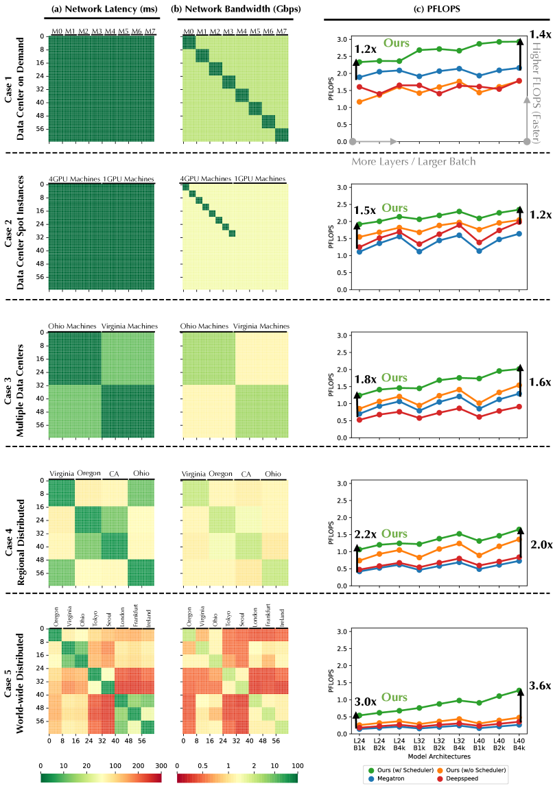
To simulate the decentralized setting, we use 8 different AWS regions (Oregon, Virginia, Ohio, Tokyo, Seoul, London, Frankfurt, and Ireland) and measure the latency and bandwidth between these regions (we consider the bandwidth that we can realistically obtain using NCCL and UDP hole punching between these regions). Given these measurements, we use 64 Tesla V100 GPUs and control their pairwise communication latency and bandwidth for five different cases:

Case 1. Data center on demand. This is a standard setting that a user can obtain to train foundation models. we use 8 AWS p3.16xlarge nodes (each with 8 V100 GPUs); the intra-node connection is NVLink of 300 GB/s bi-directional bandwidth (150 GB/s unidirectional), and the inter-node connection has a bandwidth of 25 Gbps. We do not manually control latency and bandwidth here.

Case 2. Data center spot instances. Spot GPUs are cheaper in a data center, but can be located on different types of machine. In this case, we rent 4 AWS p3.8xlarge nodes (each with 4 V100) and 32 p3.2xlarge nodes (each with 1 V100); the intra- p3.8xlarge node connection has a bandwidth of 100 Gbps, and the inter-node connection has a bandwidth of 10 Gbps. We do not manually control latency and bandwidth in this case.

Case 3. Multiple Data Centers. We consider two organizations, one in Ohio and another in Virginia, each organization contributes 32 V100 GPUs; within each organization, the bandwidth is 10 Gbps, and connections cross different campuses have a delay of 10 ms and bandwidth of 1.12 Gbps.

Case 4. Regional geo-distributed. We consider individual GPUs cross four different regions in US (California, Ohio, Oregon, and Virginia) ; within each region, the delay is 5 ms and bandwidth is 2 Gbps; cross different regions, the delay is $10{\sim}70$ms and the bandwidth is $1.0{\sim}1.3$ Gbps.

Case 5. World-wide geo-distributed. We consider individual GPUs cross eight different regions world-wide (Oregon, Virginia, Ohio, Tokyo, Seoul, London, Frankfurt, and Ireland); within each region, the delay is 5 ms and bandwidth is 2 Gbps; cross different regions, the delay is $10{\sim}250$ms and the bandwidth is $0.3{\sim}1.3$Gbps.

Metrics and Model Architecture. Since we do not introduce any optimizations that might change the computation or convergence, we can compare all methods by its throughput, we can compare all systems by the total number of floating point operations per second (PFLOPS), which is inverse proportional to the runtime of each iteration (which we show in Appendix). We use the standard GPT3-1.3B architecture Brown et al. (2020), while also benchmarked different number of layers $\{24,32,40\}$, and batch sizes $\{1024,2048,4096\}$.

Tuning of Megatron and Deepspeed. We did a careful grid search of different parallelism settings and report the optimal results in each case—in Case 1, the optimal setting includes tensor model parallelism in Megatron and ZeRO-S3 in Deepspeed; in all other cases, the optimal settings are based on pipeline and data parallelism. We discuss more details in Appendix.

4.2 Results

End-to-end Comparison.

Figure 3(c) shows the end-to-end comparison in terms of averaged PFLOPS achieved across different settings and different batch sizes and number of layers. In the world-wide geo-distributed cases, we achieve an $4.8\times$ speedup of Megatron, ($3.6\times$ speedup of Deepspeed). While in all other cases, our system can be $1.2-2.5\times$ faster. If we compare our system in Case 5 (world-wide geo-distributed) and Megatron/Deepspeed in Case 1 (data center on demand), it is exciting to see that the performance slowdown caused by decentralization is only $1.7-3.5\times$! This illustrates the great potential of decentralized training for foundation models. Additionally, Figure 3(c) illustrates another interesting behavior pattern. As increasing the batch size does not increases the communication cost of data parallelism and increasing # layers per device does not increases the communication cost of pipeline parallelism, with a larger batch size and a deeper model, the gap between centralized Megatron/Deepspeed and our decentralized system is even smaller.

Figure 4: Comparison of Search Strategies.

Effectiveness of Scheduler.

To evaluate the effectiveness of the scheduler, we disable it and use a random assignment in all cases and the results are also illustrated in Figure 3(c). We see that with our scheduler provides up to $2.7\times$ speeds up. To evaluate our local search strategy, we also compare our scheduler with a scheduler that uses the standard Kernighan-Lin algorithm for local search, illustrated in Figure 4. We see that, while both outperform random, our carefully designed local search strategy significantly outperforms Kernighan-Lin.

5 Related Work

Foundation models. Foundation modelsBommasani et al. (2021) refer to models that are trained on large-scale data and can be adapted (e.g., fine-tuned) to a wide range of downstream tasks. Current examples include BERT Devlin et al. (2018), GPT-3 Brown et al. (2020), and CLIPRadford et al. (2021). Foundation models are usually trained in a data center, where the connection between GPUs is fast and homogeneous. ML infrastructures such as MegatronShoeybi et al. (2019) and ZeRORajbhandari et al. (2020); Ren et al. (2021) have been proposed to distribute the training of these foundation models in a data center. Megatron uses AllReduce to synchronize activations in tensor model parallelism; ZeRO adopts ScatterGather to dispatch sharded parameters for layer-wise data parallelism. However, such collective communication paradigms would cause serious performance problems with slow and heterogeneous connections (see Appendix for detailed discussions).

Decentralized optimization. Decentralized training is first proposed within the scope of data parallelism, where each worker only synchronizes gradients with its neighbors (instead of all workers) to remove the latency bottleneck Koloskova et al. (2019); Li et al. (2018); Lian et al. (2017, 2018); Tang et al. (2018a, b). Recently, Diskin et al. (2021); Ryabinin et al. (2023) has also modified the implementation of data or pipeline parallelism to support training in an open collaborative environment. Varuna Athlur et al. (2022) is released by Microsoft to support the training of GPT models in spot instances from a cloud service provider, which has the potential to be extended to the open collective scenario, but there is limited consideration with respect to the challenges of heterogeneous connections.

Volunteer computing. Distributing computationally intensive tasks over an open collaborative environment has been advocated for a few decades since the development of BOINCAnderson (2004); for example, the folding@home project Shirts and Pande (2000) has been running simulations about protein dynamics on volunteers’ personal computers for more than 20 years. Recently, the learning@home projectRyabinin and Gusev (2020) starts to consider training of mixture-of-expert transformers in such a volunteer computing setting.

6 Conclusion

In this paper, we probe the opportunity to train foundation models via a decentralized training regime with devices connected over a heterogeneous network. We propose an effective scheduling algorithm to assign tasklets from the foundation model pre-train computation. Empirical studies suggest that, in the worldwide geo-distributed scenario, our proposed scheduling algorithm enables a $4.8\times$ speed-up compared to prior state-of-the-art training systems. We believe that the decentralization and democratization of the training of FMs can shift the balance of power positively, but also necessitate new governance structures to help ensure the responsible development and deployment of FMs.

7 Social Impact of Decentralized Training

In this paper, we find that decentralized training shows great potential for foundation models — such a technique would lead to significant positive social impacts. For example, decentralized training can utilize more inexpensive computational resources, which can significantly reduce the budget for the training of foundation models. This would increase the accessibility of foundation models for small research and commercial institutions. In fact, if the expense would be significantly reduced, large organizations would also receive some benefit from adopting such technology. On the other hand, we also notice that decentralization and democratization can also lead to a lack of control of cheaper computing resources and accelerate the risks of foundation models Bommasani et al. [2021]. We look forward to actively engaging the community on governance questions.

8 Limitation and Future Work

There are still some limitations of the current approach that could be explored further in future work.

First, we assume a homogeneous compute GPU resource in the scheduling algorithm, and in practice, different types of GPU could join the training computations. A native extension of the current solution could be to further split the tasklets into smaller pieces and to assign different numbers of pieces in different types of GPUs considering their memory budget and compute power as constraints. However, there are many opportunities for further improvement.

Second, there is still lots of room for the improvement of our scheduling algorithm, and strengthen our argument about the end-to-end speedup. In this paper, we hope to first provide some positive insights to the community that the potential of decentralized training can make it deployable for giant foundation models. On the other hand, there are many recent advances in system optimization that could lead to further improvement. For example, exploring recent advances in reinforcement learning Shyalika et al. [2020] to solve our scheduling algorithm would be an interesting future direction. We believe that any improvement there can only improve the decentralized performance, which is consistent with the central message we try to share in this paper.

Last but not least, there are still some important open questions on the system side to handle the dynamics in decentralized environments. For example, some mechanism should be necessary to handle the dynamic join and leave of GPU nodes. On the other hand, failure happens more frequently in the decentralized environment, as fault tolerance should be considered for deployment, we believe that the current strategy such as checkpointing the model periodically could be adopted for this problem, but there would be some suitable solutions for the decentralized training runtime.

9 Anatomy of the Current ML Systems for Foundation Model Training

Training foundation models Bommasani et al. [2021] is a challenging task due to the enormous scale of such models — even the most powerful GPU cannot hold a complete copy of parameters for such models Smith et al. [2022]. Thus, one cannot train such a model without distribution or using vanilla data parallelism.

Two popular approaches have been proposed to distribute the training of such foundation models in a data center:

• Megatron Shoeybi et al. [2019] distributes training by combining its proposed tensor model parallelism with pipeline parallelism Huang et al. [2019], Narayanan et al. [2019] and data parallelism Li et al. [2020]. The tensor model parallelism partitions individual layers across a group of workers and must run one AllReduce for the output activations of each layer in forward propagation and one AllReduce for the corresponding gradients in backward propagation for each layer.

• ZeRO Rajbhandari et al. [2020] can be viewed as an effective optimization for data parallelism. The most effective mode is called ZeRO stage-3 from the Deepspeed implementation Rasley et al. [2020], and the equivalent implementation is known as Fully Sharded Data Parallelism (FSDP) from Fairscale Baines et al. [2021]). In this mode, the parameter is sharded among all workers — in forward propagation, each worker conducts one AllGather to collect the parameters demanded for the current layer and discard the parameter after the forward computation; in backward propagation, each worker uses one AllGather to collect the parameter again and run one ReduceScatter to synchronize the gradients of this layer after the backward computation.

Both Megatron and ZeRO take a heavy usage of collective communication paradigms Chan et al. [2007], which leads to two fundamental problems when it is deployed with heterogeneous and slow connections:

• Demanding high bandwidth connections. Both Megatron and ZeRO require high bandwidth connections for collective communications, since the compute cores are idled during communication slots. As long as communication takes an increasing share (due to lower bandwidth) of the execution time, the hardware efficiency drops dramatically. In fact, tensor model parallelism is recommended only within a single DGX server equipped with high-bandwidth NVLinks Smith et al. [2022].

• Sensitive to straggler. The design and implementation of state-of-the-art collective communication libraries, e.g., NCCL ncc , assume highly homogeneous connections within a data center, thus there is not sufficient robustness to handle the straggler among workers due to the heterogeneity of the open collective runtime. Furthermore, the layer-wise usage of collective communications in both Megatron and ZeRO has intensified this problem.

To bridge the performance gap between the data center and the decentralized open environment, we need to rethink the communication paradigms in different parallel strategies.

• Pipeline parallelism is communication efficient. Pipeline parallelism Huang et al. [2019], Narayanan et al. [2019, 2021] partitions the model into multiple stages and a batch into multiple mini-batches, where once a worker finished the forward computation of a micro-batch, this worker will send the activations to the worker running the next stages; on the other hand, a worker needs to send the gradients of the activation back to the last stage in the backward propagation. Notice that pipeline parallelism utilizes point-to-point communications instead of collective paradigms. As long as one can put an increasing amount of computation inside a stage, the ratio of communication cost will also drop, leading to more efficient utilization of compute cores. On the other hand, pipeline parallelism has its own limitation — one can only partition a model to a limited number of stages, which cannot scale out to lots of GPUs. We need to combine pipeline parallelism with data parallelism to scale out the training.

• Scheduling is essential. The point-to-point communication pattern in pipeline parallelism provides good opportunities to assign the training procedure on the decentralized environment that utilizes fast links and avoids slow links by a carefully designed scheduler, as presented in Section 3.

10 Additional Details of Experimental Evaluation

We enumerate some additional details about our experiments.

10.1 Multiple Execution of the Benchmark

We repeated all the benchmarks of 5 different scenarios listed in Section 4 three times. For our system with scheduler, since the scheduled layout is the same, we simply issued three independent executions in each scenarios; For our system without scheduler, we used three different random seeds (2022, 2023, 2024) to generate three layouts, and issued one execution for each layout in each scenario. The number in Figure 3 is based on an average of three different runs for each scenario — to avoid visual confusion, we did not plot the error bar within this line plot. We also repeated the scheduling algorithms three times with random seeds (0, 1, 2) to generate scheduled layouts and reported the average estimated cost (seconds) in Figure 4. In Figure 6, we plot runtime of each iteration as a bar chart with error bars. Notice that the variance of all executions in each setting is within $5\%$.

10.2 Tuning of Megatron and Deepspeed

Megatron. We carefully tuned Megatron to perform a fair comparison with our system. As we mentioned in Section 9. Megatron has three free degrees of parallel strategies: tensor model parallelism, pipeline parallelism, and data parallelism, we note the degrees of these parallel strategies as $D_{\textsc{tp}}$, $D_{\textsc{pp}}$, and $D_{\textsc{dp}}$ respectively. We conduct a complete grid search of the combinations of these hyper-parameters in the space of:

$$\left\{\left(D_{\textsc{tp}},D_{\textsc{pp}},D_{\textsc{dp}}\right)|D_{\textsc{tp}},D_{\textsc{pp}},D_{\textsc{dp}}\in\{1,2,4,8\}\text{ and }D_{\textsc{tp}}\times D_{\textsc{pp}}\times D_{\textsc{dp}}=64\right\}.$$

And we reported the optimal setting as the results for Megatron. Interestingly, only in Case 1 (data center on demand), the optimal setting includes tensor model parallelism (i.e., $D_{\textsc{tp}}\neq 1$), where $D_{\textsc{tp}}=2,D_{\textsc{pp}}=4,D_{\textsc{dp}}=8$; in all other scenarios, the optimal setting is $D_{\textsc{tp}}=1,D_{\textsc{pp}}=8,D_{\textsc{dp}}=8$. This illustrates that tensor model parallelism is not suitable in slow and heterogeneous settings, consistent with our analysis in Section 9. Since Megatron does not include a similar scheduler as its own components, we use the same random layouts as what we test for our system without scheduler.

Deepspeed. To run Deepspeed, we start with ZeRO-S3, which is usually viewed as the most significant technical contribution of the Deepspeed system. Under the same settings, the execution time of ZeRO-S3 is much longer comparing to both Megatron and our system (See Figure 5). This is consistent with our analysis in Appendix B. We then try to combine the pipeline parallel implementation in Deepspeed with its different implementations of data parallelism (e.g., ZeRO-S 1, 2 and 3)—it turns out that even the latest version of Deepspeed (0.6.7) only allows ZeRO-S1 to combine with pipeline parallelism. We find this combination outperforms ZeRO-S3 in most of the settings in Case 1 and all settings in Case 2,3,4 and 5. Notice that results of Deepspeed we report in Figure 3 is based on the optimal result of these two settings.

Figure 5: The performance of ZeRO-S3 from Deepspeed in terms of runtime of each iteration in 5 different Scenarios.

10.3 Network Benchmark.

To obtain the network delay and bandwidth between different regions across the world, we rent AWS instances in 9 different data centers (California, Oregon, Virginia, Ohio, Tokyo, Seoul, London, Frankfurt, and Ireland). Instead of using AWS VPC, we setup our own VPN (using StrongSwan str ) established on the public IP of these instances—any GPU machine connected to Internet can be linked in the same way. The strongSwan VPN would expose a private IP associated with a visible network interface, we can bind the NCCL communication on this network interface. The delay and bandwidth we obtained for cross-region NCCL connections are summarized in Table 1 for Case 4 regional geo-distributed scenario and and Table 2 for Case 5 world-wide geo-distributed scenario.

Delay (ms)
	California	Ohio	Oregon	Virginia
California	-	52	12	59
Ohio	52	-	49	11
Oregon	12	49	-	67
Virginia	59	11	67	-
Bandwidth (Gbps)
	California	Ohio	Oregon	Virginia
California	-	1.02	1.25	1.05
Ohio	1.02	-	1.10	1.12
Oregon	1.25	1.10	-	1.15
Virginia	1.05	1.12	1.15	-

Table 1: Delay (in milliseconds) and bandwidth (in Gbps) obtained by NCCL for Case 4 regional distributed scenario.

Delay (ms)
	Oregon	Virginia	Ohio	Tokyo	Seoul	London	Frankfurt	Ireland
Oregon	-	67	49	96	124	136	143	124
Virginia	67	-	11	143	172	76	90	67
Ohio	49	11	-	130	159	86	99	77
Tokyo	96	143	130	-	34	210	235	199
Seoul	124	172	159	34	-	238	235	228
London	136	76	86	210	238	-	14	12
Frankfurt	143	90	99	235	235	14	-	24
Ireland	124	67	77	199	228	12	24	-
Bandwidth (Gbps)
	Oregon	Virginia	Ohio	Tokyo	Seoul	London	Frankfurt	Ireland
Oregon	-	1.15	1.10	0.523	0.46	0.42	0.404	0.482
Virginia	1.15	-	1.12	0.524	0.500	0.364	1.02	1.05
Ohio	1.10	1.12	-	0.694	0.529	1.05	0.799	1.14
Tokyo	0.523	0.524	0.694	-	1.1	0.366	0.36	0.465
Seoul	0.46	0.500	0.529	1.1	-	0.342	0.358	0.335
London	0.42	0.364	1.05	0.366	0.342	-	1.14	1.09
Frankfurt	0.404	1.02	0.799	0.36	0.358	1.14	-	1.08
Ireland	0.482	1.05	1.14	0.465	0.335	1.09	1.08	-

Table 2: Delay (in milliseconds) and bandwidth (in Gbps) obtained by NCCL for Case 5 world-wide distributed scenario.

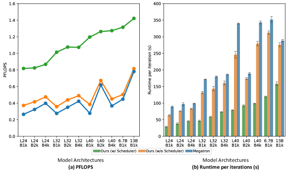
10.4 Other Presentation of Experimental Results

In Figure 6, we plot runtime of each iteration for each scenario; this is a supplement to Figure 3.

Figure 6: End to end compassion of in terms of runtime of each iteration in 5 different scenarios. We illustrate the comparison of Megatron, Deepspeed and our system with and without scheduler.

10.5 Deployment on FluidStack

We believe that having more realistic measurements and an end-to-end run can provide more pervasive statements for decentralized training. To this end, we conducted an additional experiment.

We rent 32 A40 GPUs (each with 48GB GPU memory, and 149.7 peak FP16 TFLOPS) from FluidStack flu , which consists of a group of geo-distributed GPU clusters, in (1) US Mid and (2) US East. We get the communication delay and bandwidths between GPUs as below:

• Intra-US Mid: delay $0.5_{\pm 0.1}$ ms; bandwidth $10.40_{\pm 1.11}$ Gbps;

• Intra-US East: delay $0.5_{\pm 0.1}$ ms; bandwidth $11.98_{\pm 1.92}$ Gbps;

• US Mid to US East: delay $21.8_{\pm 0.3}$ ms; bandwidth $3.87_{\pm 1.07}$ Gbps;

• US East to US Mid: delay $21.8_{\pm 0.3}$ ms; bandwidth $3.73_{\pm 1.38}$ Gbps.

We conducted an end-to-end run of the same training task of GPT3-1.3B without artificially controlling the bandwidth and latency. We also explore the training tasks of larger scale GPT3 models, including GPT3-6.7B, and GPT3-13B with a batch size of 1024. The performance in terms of the total number of floating point operations per second (PFLOPS) and runtime of each iteration are illustrated in Figure 7. This is a promising result of decentralized training — for GPT3-1.3B model with 40 layers and 4K batch size, we archive $27.4\%$ of the peak FLOPS of the cluster, for GPT3-6.7B and GPT3-13B, we obtain $26.4\%$ and $29.7\%$ respectively.

Figure 7: End to end compassion of in terms of the cluster’s whole PFLOPS in (a) and runtime of each iteration in (b). We illustrate the comparison of Megatron and our system with and without scheduler.

References

- Bommasani et al. [2021] Rishi Bommasani, Drew A Hudson, Ehsan Adeli, Russ Altman, Simran Arora, Sydney von Arx, Michael S Bernstein, Jeannette Bohg, Antoine Bosselut, Emma Brunskill, et al. On the opportunities and risks of foundation models. arXiv preprint arXiv:2108.07258, 2021.
- Brown et al. [2020] Tom Brown, Benjamin Mann, Nick Ryder, Melanie Subbiah, Jared D Kaplan, Prafulla Dhariwal, Arvind Neelakantan, Pranav Shyam, Girish Sastry, Amanda Askell, et al. Language models are few-shot learners. Advances in neural information processing systems, 33:1877–1901, 2020.
- Chowdhery et al. [2022] Aakanksha Chowdhery, Sharan Narang, Jacob Devlin, Maarten Bosma, Gaurav Mishra, Adam Roberts, Paul Barham, Hyung Won Chung, Charles Sutton, Sebastian Gehrmann, et al. Palm: Scaling language modeling with pathways. arXiv preprint arXiv:2204.02311, 2022.
- Shoeybi et al. [2019] Mohammad Shoeybi, Mostofa Patwary, Raul Puri, Patrick LeGresley, Jared Casper, and Bryan Catanzaro. Megatron-lm: Training multi-billion parameter language models using model parallelism. arXiv preprint arXiv:1909.08053, 2019.
- Rasley et al. [2020] Jeff Rasley, Samyam Rajbhandari, Olatunji Ruwase, and Yuxiong He. Deepspeed: System optimizations enable training deep learning models with over 100 billion parameters. In Proceedings of the 26th ACM SIGKDD International Conference on Knowledge Discovery & Data Mining, pages 3505–3506, 2020.
- Baines et al. [2021] Mandeep Baines, Shruti Bhosale, Vittorio Caggiano, Naman Goyal, Siddharth Goyal, Myle Ott, Benjamin Lefaudeux, Vitaliy Liptchinsky, Mike Rabbat, Sam Sheiffer, et al. Fairscale: A general purpose modular pytorch library for high performance and large scale training, 2021.
- Xu et al. [2021] Yuanzhong Xu, HyoukJoong Lee, Dehao Chen, Blake Hechtman, Yanping Huang, Rahul Joshi, Maxim Krikun, Dmitry Lepikhin, Andy Ly, Marcello Maggioni, et al. Gspmd: general and scalable parallelization for ml computation graphs. arXiv preprint arXiv:2105.04663, 2021.
- Zheng et al. [2022] Lianmin Zheng, Zhuohan Li, Hao Zhang, Yonghao Zhuang, Zhifeng Chen, Yanping Huang, Yida Wang, Yuanzhong Xu, Danyang Zhuo, Joseph E Gonzalez, et al. Alpa: Automating inter-and intra-operator parallelism for distributed deep learning. arXiv preprint arXiv:2201.12023, 2022.
- Li et al. [2021] Zhuohan Li, Siyuan Zhuang, Shiyuan Guo, Danyang Zhuo, Hao Zhang, Dawn Song, and Ion Stoica. Terapipe: Token-level pipeline parallelism for training large-scale language models. In International Conference on Machine Learning, pages 6543–6552. PMLR, 2021.
- Rajbhandari et al. [2020] Samyam Rajbhandari, Jeff Rasley, Olatunji Ruwase, and Yuxiong He. Zero: Memory optimizations toward training trillion parameter models. In SC20: International Conference for High Performance Computing, Networking, Storage and Analysis, pages 1–16. IEEE, 2020.
- Ren et al. [2021] Jie Ren, Samyam Rajbhandari, Reza Yazdani Aminabadi, Olatunji Ruwase, Shuangyan Yang, Minjia Zhang, Dong Li, and Yuxiong He. ZeRO-Offload: Democratizing Billion-Scale model training. In 2021 USENIX Annual Technical Conference (USENIX ATC 21), pages 551–564, 2021.
- [12] Q4’21 sees a nominal rise in gpu and pc shipments quarter-to-quarter. https://www.jonpeddie.com/press-releases/q421-sees-a-nominal-rise-in-gpu-and-pc-shipments-quarter-to-quarter.
- Shirts and Pande [2000] Michael Shirts and Vijay S Pande. Screen savers of the world unite! Science, 290(5498):1903–1904, 2000.
- fol [2022] OS Statistics. https://stats.foldingathome.org/os, 2022. [Online; accessed 15-May-2022].
- [15] Gpu economics cost analysis. https://venturebeat.com/2018/02/25/the-real-cost-of-mining-ethereum/.
- Lian et al. [2017] Xiangru Lian, Ce Zhang, Huan Zhang, Cho-Jui Hsieh, Wei Zhang, and Ji Liu. Can decentralized algorithms outperform centralized algorithms? a case study for decentralized parallel stochastic gradient descent. Advances in Neural Information Processing Systems, 30, 2017.
- Koloskova et al. [2019] Anastasia Koloskova, Sebastian Stich, and Martin Jaggi. Decentralized stochastic optimization and gossip algorithms with compressed communication. In International Conference on Machine Learning, pages 3478–3487. PMLR, 2019.
- Koloskova et al. [2020] Anastasia Koloskova, Nicolas Loizou, Sadra Boreiri, Martin Jaggi, and Sebastian Stich. A unified theory of decentralized sgd with changing topology and local updates. In International Conference on Machine Learning, pages 5381–5393. PMLR, 2020.
- Ryabinin and Gusev [2020] Max Ryabinin and Anton Gusev. Towards crowdsourced training of large neural networks using decentralized mixture-of-experts. Advances in Neural Information Processing Systems, 33:3659–3672, 2020.
- Diskin et al. [2021] Michael Diskin, Alexey Bukhtiyarov, Max Ryabinin, Lucile Saulnier, Anton Sinitsin, Dmitry Popov, Dmitry V Pyrkin, Maxim Kashirin, Alexander Borzunov, Albert Villanova del Moral, et al. Distributed deep learning in open collaborations. Advances in Neural Information Processing Systems, 34:7879–7897, 2021.
- Du et al. [2021] Nan Du, Yanping Huang, Andrew M. Dai, Simon Tong, Dmitry Lepikhin, Yuanzhong Xu, Maxim Krikun, Yanqi Zhou, Adams Wei Yu, Orhan Firat, Barret Zoph, Liam Fedus, Maarten Bosma, Zongwei Zhou, Tao Wang, Yu Emma Wang, Kellie Webster, Marie Pellat, Kevin Robinson, Kathy Meier-Hellstern, Toju Duke, Lucas Dixon, Kun Zhang, Quoc V. Le, Yonghui Wu, Zhifeng Chen, and Claire Cui. Glam: Efficient scaling of language models with mixture-of-experts. CoRR, abs/2112.06905, 2021. URL https://arxiv.org/abs/2112.06905.
- Narayanan et al. [2019] Deepak Narayanan, Aaron Harlap, Amar Phanishayee, Vivek Seshadri, Nikhil R Devanur, Gregory R Ganger, Phillip B Gibbons, and Matei Zaharia. Pipedream: generalized pipeline parallelism for dnn training. In Proceedings of the 27th ACM Symposium on Operating Systems Principles, pages 1–15, 2019.
- Tarnawski et al. [2020] Jakub M Tarnawski, Amar Phanishayee, Nikhil Devanur, Divya Mahajan, and Fanny Nina Paravecino. Efficient algorithms for device placement of dnn graph operators. Advances in Neural Information Processing Systems, 33:15451–15463, 2020.
- Tarnawski et al. [2021] Jakub M Tarnawski, Deepak Narayanan, and Amar Phanishayee. Piper: Multidimensional planner for dnn parallelization. Advances in Neural Information Processing Systems, 34, 2021.
- Fan et al. [2021] Shiqing Fan, Yi Rong, Chen Meng, Zongyan Cao, Siyu Wang, Zhen Zheng, Chuan Wu, Guoping Long, Jun Yang, Lixue Xia, et al. Dapple: A pipelined data parallel approach for training large models. In Proceedings of the 26th ACM SIGPLAN Symposium on Principles and Practice of Parallel Programming, pages 431–445, 2021.
- Park et al. [2020] Jay H Park, Gyeongchan Yun, M Yi Chang, Nguyen T Nguyen, Seungmin Lee, Jaesik Choi, Sam H Noh, and Young-ri Choi. HetPipe: Enabling large DNN training on (whimpy) heterogeneous GPU clusters through integration of pipelined model parallelism and data parallelism. In 2020 USENIX Annual Technical Conference (USENIX ATC 20), pages 307–321, 2020.
- Papadimitriou [1977] Christos H Papadimitriou. The euclidean travelling salesman problem is np-complete. Theoretical computer science, 4(3):237–244, 1977.
- Kang and Moon [2000] So-Jin Kang and Byung-Ro Moon. A hybrid genetic algorithm for multiway graph partitioning. In Proceedings of the 2nd Annual Conference on Genetic and Evolutionary Computation, pages 159–166. Citeseer, 2000.
- Vaswani et al. [2017] Ashish Vaswani, Noam Shazeer, Niki Parmar, Jakob Uszkoreit, Llion Jones, Aidan N Gomez, Łukasz Kaiser, and Illia Polosukhin. Attention is all you need. Advances in neural information processing systems, 30, 2017.
- Sergeev and Del Balso [2018] Alexander Sergeev and Mike Del Balso. Horovod: fast and easy distributed deep learning in tensorflow. arXiv preprint arXiv:1802.05799, 2018.
- Jiang et al. [2020] Yimin Jiang, Yibo Zhu, Chang Lan, Bairen Yi, Yong Cui, and Chuanxiong Guo. A unified architecture for accelerating distributed DNN training in heterogeneous GPU/CPU clusters. In 14th USENIX Symposium on Operating Systems Design and Implementation (OSDI 20), pages 463–479, 2020.
- Goemans [2009] Michel X Goemans. Lecture notes on bipartite matching. Massachusetts Institute of Technology, 2009.
- Garey and Johnson [1979] Michael R Garey and David S Johnson. Computers and intractability, volume 174. freeman San Francisco, 1979.
- Andreev and Racke [2006] Konstantin Andreev and Harald Racke. Balanced graph partitioning. Theory of Computing Systems, 39(6):929–939, 2006.
- Sanders and Schulz [2013] Peter Sanders and Christian Schulz. Think locally, act globally: Highly balanced graph partitioning. In International Symposium on Experimental Algorithms, pages 164–175. Springer, 2013.
- Buluç et al. [2016] Aydın Buluç, Henning Meyerhenke, Ilya Safro, Peter Sanders, and Christian Schulz. Recent advances in graph partitioning. Algorithm engineering, pages 117–158, 2016.
- El-Mihoub et al. [2006] Tarek A El-Mihoub, Adrian A Hopgood, Lars Nolle, and Alan Battersby. Hybrid genetic algorithms: A review. Eng. Lett., 13(2):124–137, 2006.
- Bui and Moon [1996] Thang Nguyen Bui and Byung Ro Moon. Genetic algorithm and graph partitioning. IEEE Transactions on computers, 45(7):841–855, 1996.
- Devlin et al. [2018] Jacob Devlin, Ming-Wei Chang, Kenton Lee, and Kristina Toutanova. Bert: Pre-training of deep bidirectional transformers for language understanding. arXiv preprint arXiv:1810.04805, 2018.
- Radford et al. [2021] Alec Radford, Jong Wook Kim, Chris Hallacy, Aditya Ramesh, Gabriel Goh, Sandhini Agarwal, Girish Sastry, Amanda Askell, Pamela Mishkin, Jack Clark, et al. Learning transferable visual models from natural language supervision. In International Conference on Machine Learning, pages 8748–8763. PMLR, 2021.
- Li et al. [2018] Youjie Li, Mingchao Yu, Songze Li, Salman Avestimehr, Nam Sung Kim, and Alexander Schwing. Pipe-sgd: a decentralized pipelined sgd framework for distributed deep net training. In Proceedings of the 32nd International Conference on Neural Information Processing Systems, pages 8056–8067, 2018.
- Lian et al. [2018] Xiangru Lian, Wei Zhang, Ce Zhang, and Ji Liu. Asynchronous decentralized parallel stochastic gradient descent. In International Conference on Machine Learning, pages 3043–3052. PMLR, 2018.
- Tang et al. [2018a] Hanlin Tang, Shaoduo Gan, Ce Zhang, Tong Zhang, and Ji Liu. Communication compression for decentralized training. In Proceedings of the 32nd International Conference on Neural Information Processing Systems, pages 7663–7673, 2018a.
- Tang et al. [2018b] Hanlin Tang, Xiangru Lian, Ming Yan, Ce Zhang, and Ji Liu. D2: Decentralized training over decentralized data. In International Conference on Machine Learning, pages 4848–4856. PMLR, 2018b.
- Ryabinin et al. [2023] Max Ryabinin, Tim Dettmers, Michael Diskin, and Alexander Borzunov. Swarm parallelism: Training large models can be surprisingly communication-efficient. 2023.
- Athlur et al. [2022] Sanjith Athlur, Nitika Saran, Muthian Sivathanu, Ramachandran Ramjee, and Nipun Kwatra. Varuna: scalable, low-cost training of massive deep learning models. In Proceedings of the Seventeenth European Conference on Computer Systems, pages 472–487, 2022.
- Anderson [2004] David P Anderson. Boinc: A system for public-resource computing and storage. In Fifth IEEE/ACM international workshop on grid computing, pages 4–10. IEEE, 2004.
- Shyalika et al. [2020] Chathurangi Shyalika, Thushari Silva, and Asoka Karunananda. Reinforcement learning in dynamic task scheduling: A review. SN Computer Science, 1(6):1–17, 2020.
- Smith et al. [2022] Shaden Smith, Mostofa Patwary, Brandon Norick, Patrick LeGresley, Samyam Rajbhandari, Jared Casper, Zhun Liu, Shrimai Prabhumoye, George Zerveas, Vijay Korthikanti, et al. Using deepspeed and megatron to train megatron-turing nlg 530b, a large-scale generative language model. arXiv preprint arXiv:2201.11990, 2022.
- Huang et al. [2019] Yanping Huang, Youlong Cheng, Ankur Bapna, Orhan Firat, Dehao Chen, Mia Chen, HyoukJoong Lee, Jiquan Ngiam, Quoc V Le, Yonghui Wu, et al. Gpipe: Efficient training of giant neural networks using pipeline parallelism. Advances in neural information processing systems, 32, 2019.
- Li et al. [2020] Shen Li, Yanli Zhao, Rohan Varma, Omkar Salpekar, Pieter Noordhuis, Teng Li, Adam Paszke, Jeff Smith, Brian Vaughan, Pritam Damania, et al. Pytorch distributed: experiences on accelerating data parallel training. Proceedings of the VLDB Endowment, 13(12):3005–3018, 2020.
- Chan et al. [2007] Ernie Chan, Marcel Heimlich, Avi Purkayastha, and Robert Van De Geijn. Collective communication: theory, practice, and experience. Concurrency and Computation: Practice and Experience, 19(13):1749–1783, 2007.
- [53] Nccl. https://developer.nvidia.com/nccl.
- Narayanan et al. [2021] Deepak Narayanan, Amar Phanishayee, Kaiyu Shi, Xie Chen, and Matei Zaharia. Memory-efficient pipeline-parallel dnn training. In International Conference on Machine Learning, pages 7937–7947. PMLR, 2021.
- [55] Strongswan vpn. https://www.strongswan.org/.
- [56] Fluidstack. https://www.fluidstack.io/.