Inclusive Thermodynamics of Computational Machines

Abstract

We introduce a framework designed to analyze the thermodynamics of an abstractly defined logical computer like a deterministic finite automaton (DFA) or a Turing machine, without specifying any extraneous parameters (like rate matrices, Hamiltonians, etc.) of a physical process that implements the computer. Earlier investigations of how to do this were based on the continuous-time Markov chain (CTMC) formulation of stochastic thermodynamics. These investigations either assumed that there was exactly zero irreversible entropy production (EP) generated by the physical system implementing the computation, or allowed the EP to be nonzero but only considered the “mismatch cost” component of the EP. In addition, they only applied to a single type of computer. Our framework neither requires that EP equal zero nor restricts attention to the mismatch cost component of EP, and is designed to apply to all types of computational machines. In contrast to earlier investigations using the CTMC-based formulation, our framework is based on the inclusive Hamiltonian formulation, in which the combination of the system of interest and the baths evolve in a Hamiltonian (or unitary) dynamics. Here, we use our framework to derive an integral fluctuation theorem for computers, in which the expectation value is strictly less than 1. We also derive an exchange fluctuation theorem, and a mismatch cost formula involving first-passage times. We analyze the EP generated by a DFA, a Markov information source, and a noisy communication channel. In particular, we use the Myhill-Nerode theorem of computer science to prove that out of all DFAs which recognize the same language, the “minimal complexity DFA” is the one with minimal EP for all dynamics and at all iterations.

I Introduction

I.1 Background

The thermodynamic costs of computation has been a central topic of concern for physicists and mathematicians for over a century. Early work ranges from Szilard’s analyses of Maxwell’s Demon [1] to remarks by von Neumann, in which he argued that a computer operating at temperature $T$ must dissipate at least $kT\ln 2$ Joule per elementary bit operation [2]. Landauer, Bennett, Zurek, Caves and other collaborators then built on these earlier investigations with a more extended, semi-formal analysis in the mid- to late twentieth century [3, 4, 5].

All these early investigations were based on equilibrium thermodynamics. However, real-world computers almost always operate (extremely) far from thermodynamic equilibrium. This indicates that a more complete and detailed understanding of the thermodynamics of computation, extending beyond the analyses of the last century, must involve a formalism explicitly designed to apply to non-equilibrium systems.

Fortunately, the last two decades have witnessed substantial advances which have extended statistical physics to include systems operating arbitrarily far from equilibrium. One of the core ideas underlying these recent advances is to extend the definitions of thermodynamic quantities to the level of individual trajectories of a system, i.e., to define work, heat, etc., for individual samples of the stochastic process governing dynamics of that system [6]. This has allowed the derivation of powerful “fluctuation theorems” (FTs) [7, 8, 9, 10] that govern the probability density function of how much work is dissipated in a process. More recent results include “speed limit theorems” bounding how fast a thermodynamic system can change its state distribution by the amount of dissipated work it produces [11, 12, 13, 14]. Similarly, “thermodynamic uncertainty relations” (TURs [15, 16, 17, 18, 19, 20]) bound the statistical precision of any type of current within a system by the amount of dissipated work it generates. Other recent results include various bounds relating dissipated work to stopping times and first-passage times [21, 22, 23, 20, 24].

This new field is called stochastic thermodynamics (ST), and has two main approaches. Most of the research in ST has been based on considering systems of interest (SOIs) that are coupled to one or more infinite external reservoirs (also called baths). In this standard approach, the reservoirs are assumed to always be at thermal equilibrium, e.g., due to separation of timescales or coarse-graining [25, 26, 9, 27]. Therefore there is no dynamic model of the reservoirs, and typically only an indirect model of the coupling of the reservoirs to the SOI, via conditions on the allowed dynamics of the SOI. In this approach the SOI itself evolves according to a continuous-time Markov chain (CTMC) [26].

As described below, one of the central results in CTMC-based stochastic thermodynamics is a formula for the time-derivative of the Shannon entropy of distribution $p_{t}$ over the states of the SOI at time $t$:

$$\dfrac{dS(p_{t})}{dt}=\dot{Q}(p_{t})+\dot{\Sigma}(p_{t})$$ (1)

The first term on the RHS is called the “entropy flow” rate (EF). In many settings it can be identified with the rate of heat exchanged between the SOI and the reservoirs. The second term is called the “entropy production” rate (EP). Crucially, it is never negative. (In many scenarios the second law of thermodynamics is a consequence of this non-negativity.) The physical process of the system evolving according to the CTMC is thermodynamically reversible iff the EP rate equals $0$. In general, that can only occur if the process is proceeding semi-statically slowly [26].

Another substantial portion of ST research instead adopts an “inclusive Hamiltonian framework”. In this approach the external reservoirs can be finite or infinite, but they have a finite number of degrees of freedom. Moreover, it is not assumed that they are always at thermal equilibrium. Instead, a deterministic invertible dynamics is defined over the full physical system, including both the SOI and the external reservoirs. Often, it is also assumed that the initial distribution over the joint SOI-reservoirs is a product distribution, i.e., that the SOI and the reservoirs are initialized in statistically independent processes [8, 28, 29, 30, 31, 32, 33, 34].

Importantly, this Hamiltonian framework is not only applicable to classical systems. It is also one of the common ways to model open quantum systems. In those quantum models, one explicitly specifies a unitary operator governing the joint dynamics of an SOI together with the external systems coupled to the SOI, with partial traces used to evaluate the dynamics of the SOI by itself [35, 36]. This model of quantum systems is central to recent research on quantum information processing [35].

Our goal in this paper is to build on this previous work in ST, to construct a formalism for analyzing the thermodynamics of arbitrary computational systems that depends solely on the logical dynamics of those systems, without further specifying any of the low-level details of the physical process that implements that machine. We want to be able to analyze the thermodynamics of just the dynamics of the computational machine, with our conclusions not changing based on extraneous physical parameters that are not fixed by the dynamics of the computational machine.

The CTMC-based approach to ST has made some progress towards this goal. Previous research in this category has fallen into two classes:

1. In the first class, it is assumed that EP = 0 [37, 38, 39]. As mentioned above, in general this restricts us to considering systems that are evolving infinitesimally slowly. In this situation, the total EF — the total heat exchange with the reservoirs — is the change in the Shannon entropy. This allows us to derive expressions for the EF by considering only the logical computation implemented by the system, together with the initial distribution over its states, without considering any extraneous physical parameters;

2. The second class of investigations focuses on the EP, ignoring the EF [38, 40]. Specifically, these papers focus on what is called the “mismatch cost” contribution to the EP. This contribution to the EP is always non-negative. Like the EF in systems with zero EP, this contribution to the EP is determined fully by the logical computation that the system implements, together with the initial distribution over its states, without any dependence on extraneous physical parameters. Moreover, this contribution to EP is nonzero if we assume the physical system implementing the computation evolves periodically, with one iteration of the computation performed in each period. This is almost always the case in real-world computers.

These analyses have revealed that there are unavoidable trade-offs among the thermodynamic resources used in specific nonequilibrium physical systems, in particular systems that perform computation. Some of the trade-offs uncovered relate to the speed of a computation, its noise level, and whether the computational system is thermodynamically “tailored” to perform a given computational task [41, 37, 38, 42, 33, 43, 44, 45].

Figure 1: Schematic depiction of a full thermodynamic cycle of a DFA, special type of logical computer. The cycle starts with the DFA in its initial state and the environment’s state — a bit string — set to a random sample of an associated distribution, modeled as a Boltzmann distribution for a bath Hamiltonian. The forward process of the DFA occurs as the DFA reads in the input string generated by the environment. Once the DFA halts, an infinite external reservoir is connected to the DFA, and a second, independent one is connected to the environment. These external reservoirs are used to reinitialize the DFA and environment, respectively, in preparation for the next run of the DFA.

In this paper we show that by adapting the Hamiltonian framework, we can analyze the energetic costs associated with a computational task in toto, without specifying any extraneous physical parameters that are not already given in the computer science (CS) theory definition of the computation. In particular, by using this version of the Hamiltonian framework we can avoid the need for making restrictive assumptions on the speed of the process (in contrast to (1)) or for ignoring components of the energetic cost (as in (2)). In addition, our new framework applies to arbitrary computational machines. Moreover, it is based on the assumption of the Hamiltonian framework that the the states of SOI and the of the bath(s) are independent of one another when the process starts. This assumption is perfectly suited to analyzing computational machines that receive external inputs after they have been initialized — which is the case in all CS theory.

As a result of these attributes, the framework we introduce opens the possibility of analyzing the trade-offs among all of the thermodynamic resources that are consumed in any computation, in the sense of the term meant in computer science involving abstract logical variables, rather than focus on the thermodynamic resources consumed in a specific physical system that implements some specific computation.

Trade-offs among the minimal amounts of resources required to perform a given computation have not only been considered in ST. Indeed, such trade-off are a central concern of CS theory. However, traditional CS theory has considered trade-offs among quantities different from those considered in the thermodynamics of computation [46]. For instance, one of the most important examples of a trade-off considered in CS theory is the relation between the amount of memory needed by a computational machine to perform a given computation and the number of iterations required to perform that computation [47].

Despite this parallel between the interests of ST and CS theory in the trade-offs among the resource costs involved in computation, very little research has been done on how the resource costs investigated in ST are related to the resource costs so central to CS. In this paper, after introducing our framework, we use it to start to lay the foundations for investigating that relationship.

I.2 Reinitialization entropy production

Our starting point is to note that many models of computational systems can be decomposed into two or more interacting subsystems [48]. The first is the computational machine itself. Examples of such machines range from deterministic finite automata (DFAs) to Turing machines (TMs) to concurrent processes. In addition to the computational machine, there are always one or more external processes which provide inputs to and receive outputs from the computational machine.

We physically ground this decomposition by supposing that there are two types of degrees of freedoms in physical devices that implement computational machines . First, the accessible degrees of freedom are those that arise directly in the specification of the computational machine executing a well-defined computational task. As an example, in a DFA, one could take the accessible degrees of freedom to be the computational state of the DFA. Whatever our computational machine is, we suppose that there is an engineer who builds a physical device that implements that computational machine. More precisely, we suppose that they build a physical device some of whose physical variables correspond to the accessible degrees of freedom of the computational machine. So the dynamics of the physical device implements the computational task across the accessible degrees of freedom.

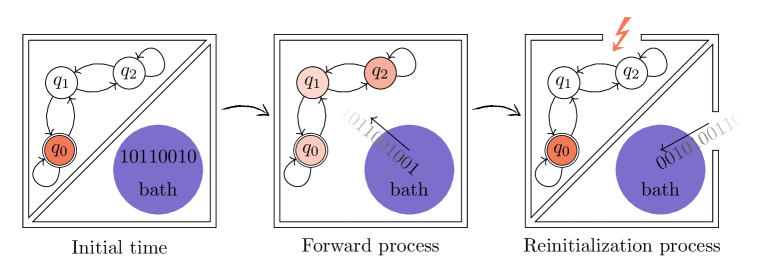
We refer to the dynamics of the full physical system as it implements a given computation as the forward process. In real world scenarios, it is expected that the engineer will use the physical device repeatedly. So after every use of the device in the forward process, the device needs to be reinitialized for its next use, as illustrated in Fig. 1. We suppose that the engineer has complete freedom to design how the physical device controls the accessible degrees of freedom during that re-initialization (hence the name “accessible”).

The dynamics of the physical device is driven by the external world which provides stochastic inputs to the device. Supposing that the distribution of those inputs is fully specified, at all times there is a well-defined probability distribution over the accessible degrees of freedom in the physical device. We suppose that the engineer knows exactly what that probability distribution is at the time that the device has completed a computation, and can use that knowledge to design a thermodynamically efficient physical process to re-initialize those accessible degrees of freedom.

Formally, as described in the following sections, these properties mean that we can lower-bound the amount of work the engineer will need to spend to re-initialize the (accessible degrees of freedom in the) computational machine. This lower bound is given by how the non-equilibrium free energy over those degrees of freedom changes, when the engineer transforms the ending distribution over the accessible degrees of freedom back to the initial distribution.

In addition to the accessible degrees of freedom, there is also a set of degrees of freedom that are inaccessible to the engineer, that comprise the external world which interacts with the computational machine. For example, in the case of a DFA, one could consider the entire string of inputs read into the DFA as being inaccessible. We suppose that the engineer knows the distribution over the inaccessible degrees of freedom when the computation halts, just like they know the distribution over the accessible degrees of freedom. However, we also suppose that the engineer has no control over how the inaccessible degrees of freedom are re-initialized. Formally, as described in the following sections, this means that we can upper-bound the amount of work the engineer can extract when the inaccessible degrees of freedom are reinitialized. This upper bound is given by the amount of heat that would be produced if those degrees of freedom were re-initialized in an uncontrolled manner, i.e., by coupling them to an idealized, infinite heat bath whose Boltzmann distribution is the initial distribution over the inaccessible degrees of freedom .

The difference between this minimal amount of work that needs to be spent (to re-initialize the accessible degrees of freedom) and the maximal amount of work that can be extracted (by re-initializing the inaccessible degrees of freedom) combine to provide a lower bound on the amount of work that will be dissipated — irretrievably lost — every time the computational machine is run. This bound applies independent of the details of the actual physical system that implements the computational machine, since by the second law of thermodynamics, those details can increase the total amount of dissipated work, but cannot reduce it.

Importantly, this bound on the expected disssipated work of the reinitialization process exactly equals the expected entropy production of the forward process [29]. Accordingly, we will refer to this bound as the expected reinitialization entropy production (REP) of the system. It is important to emphasize that the REP depends only on the thermodynamics of re-initializing the machine after it has completed a computational task. It does not reflect any extra dissipated work that arises in the forward process, while that computation runs.

From now on we will refer to the physical variables that we suppose the engineer is directly interested in, and that are accessible to them, as the system of interest (SOI). (So these are the variables in the physical device that the engineer is directly interested in.) All variables not in the physical device are considered to be inaccessible. These are partitioned into one or more baths (or reservoirs). (As illustrated below, the baths will implement the sequence of inputs into and outputs from the computer.)

Sometimes we will need to distinguish between the abstract computer together with its abstract sequence of inputs, as considered in CS, and the physical system that implements that computer together with its inputs. In such cases we refer to the former as the logical computer, and refer to the latter as the physical computer. So for example, the physical computer comprises the SOI and the set of all the baths.

A key part of our framework is a coordinate transformation between states of the logical computer and those of the physical computer. However, when care to distinguish those two types of computer is not needed, we will sometimes just use the term computational system, implicitly relying on context to determine whether we mean the logical computer or the physical computer. We will also sometime use the term computational machine to refer to that part of the computational system that does not involve the inputs, again relying on context to determine whether we mean the SOI or the abstract, mathematical computer that the SOI implements.

I.3 The forward processes

To investigate the thermodynamics of the forward process, we need to specify the initial distribution over the set of all the variables in the computational system, both those in the SOI and those in the baths. Often this step is skipped in CS, since that distribution is not relevant to the questions being investigated. However, this step is crucial for us. Indeed, when combined with the dynamics of the full computational system, that initial distribution fixes the final distribution — and it is the relation of those two distributions that determines the value of the EP.

Typically in computational models, if the initial distribution over the full computational system is in fact specified, it is a product distribution over the SOI and the bath(s). Concretely, it is almost always the case in those analyses that the initial state of the computational machine is statistically independent of the initial state of the external world generating the stream of inputs. Accordingly, in our analysis we presume that the joint physical system is initially in a product distribution.

Next, we need to specify the dynamics of the physical computer during the forward process, starting from such a product distribution. We suppose that the dynamics during the forward process is logically reversible (and therefore deterministic). There are three reasons for this:

• Define the “physical computer EP” (PEP) to be the EP that would be generated by a physical computer that completes a given computation. There are infinitely many Markov processes that could be used for that physical computer and that are thermodynamically reversible, resulting in zero PEP. In particular, a deterministic and reversible process is such a Markov process. These processes have a special property though: by the mismatch cost theorems [51], any forward process that generates zero PEP for one initial distribution over the joint system will also generate zero PEP if run with a different initial distribution if that process is reversible and deterministic. In contrast, if the forward process is non-invertible, then it is possible to implement it with zero PEP only for one specific initial distribution. Moreover, the mismatch cost theorem also establishes that any other initial distribution for such a non-invertible dynamics will generate strictly positive PEP, no matter what the precise form of that (non-invertible) dynamics.

  In other words, if the forward process is non-invertible, then in general there must be nonzero dissipated work if one does not initialize the full system with the unique initial “prior” distribution of the (full system) physical process. Moreover, the precise amount of that dissipated work will depend both on the actual distribution and on the prior distribution. Accordingly, one cannot calculate PEP without specifying that prior distribution for such a stochastic process.

  The prior distribution is in turn specified by the precise details of the physical computer, details that have nothing to do with they dynamics of the logical computer. The result is that for such non-invertible stochastic processes, we cannot calculate the PEP without specifying some of those precise details of the physical computer which are absent in the associated logical computer. In contrast, a physical computer that has invertible dynamics can generate zero PEP no matter what the initial distribution and prior distributions are.

  This means we can ignore the issue of what the prior distribution is — so long as the dynamics is invertible. So by using an invertible dynamics we can focus on the thermodynamics arising from just the logical computer, without concern for the parameters of the underlying physical process that implements that computer.

• Many of the machines considered in CS theory are deterministic, and many are stochastic. We want our framework to be able to represent systems with either kind of dynamics in a straightforward way. As we show below, this can be done if we restrict attention to systems with deterministic dynamics. In particular, it is straightforward to implement an arbitrary stochastic evolution of the SOI using a fully deterministic and invertible joint system. (This can be done by using the random initialization of the baths to introduce stochasticity into the dynamics of the SOI as and when needed.)

• Another advantage of our using deterministic, invertible dynamics of a system is that if the full system, including the baths, has only a finite number of degrees of freedom, then we are in precisely the setting of the inclusive Hamiltonian framework, mentioned above. This means in particular that our results should carry over with minor modifications to the quantum thermodynamics of open quantum systems. (In contrast, there are nontrivial difficulties in formulating the dynamics of the SOI in open quantum systems in terms of CTMCs, which substantially restricts our ability to analyze such systems using the CTMC-based version of stochastic thermodynamics.)

  Accordingly, to complement our analysis of the REP, below we also present some new results concerning the PEP as defined under the Hamiltonian framework of the forward process; we refer to this quantity as the HEP (Hamiltonian framework EP).

First, we show below that the expected value of the HEP equals the expected value of the REP. Next, we derive an integral fluctuation theorem (IFT) and an exchange FT (XFT) for the HEP. As a final contribution to understanding of the HEP, we confirm that the mismatch cost formula holds for the HEP .

I.4 Results and roadmap

We refer to this minimal model of the thermodynamics of a computational machine and its external environment during a forward process followed by a reinitialization process as the inclusive thermodynamics of computational machines.

At a high level, we have two sets of results concerning inclusive thermodynamics:

1. Some of our results concern the the thermodynamics of the forward process, considered from the perspective of the Hamiltonian framework, adapted to computational machines. We emphasize that these results are actually more general than our analysis of computational machines, as they apply to any use of the Hamiltonian framework. Specifically, we have derived the mismatch cost formula for the Hamiltonian framework, and also an IFT and an XFT within this framework.

2. One might be concerned about the applicability of the Hamiltonian framework particularly to systems like DFAs, since that framework would only apply if we could assume that input strings to the DFA were generated by repeatedly sampling a Boltzmann distribution: in the real world, input strings are generated by engineers. Accordingly, we consider a lower bound on the expected dissipated work of the reinitialization process. We show that the lower bound derived this way –which is the REP– also lower bounds the EP of the Hamiltonian framework. Hence, all our results concerning a lower bound on the expected dissipated work in the reinitialization process of an inclusive model of a computational machine also apply to the HEP of that machine.

More specifically, in this paper, we employ our framework to investigate the dissipation costs of three computational systems:

1. DFA, which is a foundational model of computation that underlies more general models such as the TM,

2. Markov sources of information theory,

3. Communication channels central to the theory of communication.

Our paper is organized as follows: In Section II, we provide the elementary concepts of the inclusive framework. In Section III, we formally define the three different computational systems we analyze in this paper. In Section IV, we present the mathematical basis for our framework. In Section IV.2, we develop the inclusive thermodynamics of DFAs and derive the lower bound on dissipated work as REP. In Section V.2, we use a special class of DFAs to model Markov information sources. In Section V.5, we extend Section V.2 to model communication channels. Subsequently in Section V.7, we formulate the rate-distortion problem in the theory of communication using the inclusive thermodynamic quantities.

In Section V.3, Section V.4, and Section V.8 we present our results concerning the thermodynamics of the forward processes of physical computers which implement DFAs. In Section V.3 we derive an IFT for the HEP. In contrast to conventional IFTs though, here we find that the expectation of (the exponential of negative of the) HEP is upper-bounded by $1$, rather than equal $1$ exactly, as it is the case in conventional IFTs. Intuitively, this is because typically the logical computers considered in CS theory have a single, unique initial state. So the distribution over the states of the SOI at $t=0$ is a delta function. This means that any reverse trajectory that does not end in that initial state does not contribute to the IFT calculation. In other words, the IFT we derive equals $1$ minus the probability of such an impossible reverse trajectory. In Section V.4, we derive a mismatch cost result concerning the PEP of the Hamiltonian framework. We derive our mismatch cost result with respect to marginal distribution over the states of the SOI, so it differs from the mismatch cost of the full system discussed in Section I.3. Next in Section V.8, we extend a previously derived XFT for the HEP to scenarios with multiple baths.

In the remaining sections, we analyze the connections between a CS measure of complexity over DFAs and the EP of executing DFAs. We prove in Section V.9.2 that for equivalent DFAs with different size complexities, executing a minimal complexity DFA results in the minimal EP at all iterations.

We conclude with a discussion, where we describe methods and features essential to both CS and inclusive thermodynamics. We describe a few research directions where our framework might prove fruitful.

As we will later come back in Section VII, we are interested in implementing our framework to analyze many computational systems, ranging from push-down automata to TMs. In this work, we mainly focus on introducing the framework and illustrating it through computational systems which can implement DFAs.

II General framework: Inclusive formulations of computational systems

We will consider physical systems which evolve in discrete time. These systems have at least two components: an SOI, and a set of one or more external environments which interact with the SOI, and are referred to as baths. The discrete time physical forward processes will evolve the joint system of the SOI and the bath(s) from an initial joint distribution, until some ending condition is reached (i.e., until computational task is implemented fully). After that the joint distribution is reinitialized, to start a next physical forward process, where another computational task is implemented. We use the term computational cycle to mean such an entire process, taking the physical system from one initialized distribution to the next.

As an example, much of our analysis below concerns DFAs, a special type of logical computer. Loosely speaking, a DFA is a system with a finite state space $S$, having elements $s$. Initially the DFA is initialized to a special “start state”. After that it receives a sequence of exogeneously generated symbols called a “string”. Those symbols are all elements of a finite alphabet, $\Sigma$ (e.g., the binary alphabet $\Sigma_{0,1}$). As the DFA iteratively receives those symbols it makes associated transitions among its possible states. The state of the DFA when a termination condition is reached (e.g., when the string ends) defines the computation that the DFA performs on that string it received. After it performs such a computation, the DFA is reinitialized in its start state. (See Section III for the formal definition of a DFA.)

We write a generic symbol from $\Sigma$ as $y$. In this paper, we suppose that $\Sigma$ includes a special blank symbol “$\varepsilon$”. As usual, we denote the set of finite strings of symbols from the alphabet as $\Sigma^{*}$ [48]. We write a string that a DFA receives as $\omega$, having length $|\omega|$. In our simplest physical model of the DFA, we identify the state of the DFA as the state of the SOI, and the string $\omega$ with the state of the bath. In this version we consider below, the state of the bath does not change during a computational cycle. This has two consequences. First, it means that we identify the initial distribution of the state of the bath with the distribution over strings that will be received by the DFA. Moreover, it means we must augment the state space of the SOI. In addition to specifying the state of the DFA, the state of the SOI must specify an integer-valued pointer, $z$, to keep track of which element of the string $\omega$ is the current one. In other words, $z$ gives the iteration time $t$ at which the symbol $\omega[z=t]=y$ is received by the DFA. For later convenience, we define $\omega[-z]$ to mean the string of symbols of $\omega$ that are not read at iteration $t=z$, $\omega[t=1]\dots\omega[t=z-1]\omega[t=z+1]\dots\omega[t=|\omega|]$.

In this simple implementation of a DFA, the state space of the full computational system is the set of all triples $(s,z,\omega)$. For the reasons given above, we suppose that the dynamics governing this full space is deterministic. We will let strings $\omega$ be sampled at the beginning of each computational cycle, so that $\omega$ is time independent, and it is always possible to reconstruct the past history of a DFA’s states. As a result, any distribution over the full state evolves by permuting which state has which probability, but doesn’t actually change the multiset of the probability values of all joint states. Since entropy is a unique function of that multiset of probability values, this means that the entropy over the full state space is constant in time.

In order to investigate the associated thermodynamics, we must explicitly decompose the full state space into a Cartesian product of two spaces: the set of states of the SOI and the set of states of the bath. The states of the SOI contain the accessible degrees of freedom, whereas the states of the bath are those inaccessible degrees of freedom.

As pointed out in Section I.2, we assume that the state of the SOI is “accessible” to the engineer once the DFA has completed a run. This implies that the engineer is allowed to reinitialize the initial distribution of SOI states by implementing any desired external work protocol over the SOI, while the SOI is coupled to an infinite external thermal reservoir at temperature $1/k_{B}$. In addition, as is conventional in the ST literature of information processing, we assume that the Hamiltonian of the SOI is uniform at both the beginning and end of any run, with the same value at those two times [39]. More precisely, we say that there is a constant $\mathrm{A}$ such that both the Hamiltonian of the SOI at the beginning of the run and at end of the run have the value $\mathrm{A}$, independent of the state of the SOI.

Based on these two assumptions, we can exploit the generalized Landauer bound of modern ST: the minimal free energy needed for re-initializating an SOI is given by the change in the entropy (of the distribution over states) between the SOI’s ending distribution and its re-initialized distribution .

For the reservoirs, we assume that their states are “inaccessible” to the engineer once the DFA has completed a run. Suppose that at the end of the computational process, the distribution over states of the bath is re-initialized, just like the distribution over states of the SOI. Since the states of the bath are inaccessible, the engineer will not be able to implement this reinitialization in a thermodynamically optimal manner. We suppose that the maximal free energy that can be extracted in this reinitialization of the bath distribution would occur by the bath’s relaxing to the thermal equilibrium of a fixed Hamiltonian, while being coupled to to an infinite external thermal reservoir at temperature $1/k_{B}$. This Hamiltonian is chosen so that the associated Boltzmann distribution is the desired initial distribution of bath states at the beginning of the subsequent run. As opposed to the re-initialization of the SOI distribution, the engineer is not allowed to implement any external work protocol acting on the bath distribution as it is reinitialized.

III Preliminaries

In this section we provide the definitions of DFAs, Markov information sources, and communication channels, as they are used in our paper.

III.1 Basic concepts and terminology

III.1.1 Regular languages and finite automata

A deterministic finite automaton (DFA) is a five-tuple $M=\left(S,\Sigma,f,q_{0},K\right)$, where $S$ is a finite set of states, $\Sigma$ is a finite alphabet of observable symbols, $f:S\times\Sigma\rightarrow S$ is a transition function mapping a current input symbol and the current state to another state, $q_{0}$ is a start state, and $K$ is a set of accepting states. An input string $\omega$, i.e. a sequence of symbols from $\Sigma$, is accepted by a DFA if the last state entered by the machine on that input string is in $K$. A language recognized by a DFA is the set of strings that it accepts, $L(M)=\{\omega\in\Sigma^{*}\mid{f}\left(q_{0},w\right)$ $\in$ $\left.K\right\}$. Equivalently, the language of a DFA is the decision problem it solves . $L$ is a regular language if there is a DFA $M$ which recognizes $L$.

Given a language $L\subseteq\Sigma^{*}$, a pair of strings $a,b\in\Sigma^{*}$ are equivalent with respect to $L$, i.e. $a\sim_{L}b$, if for all $w\in\Sigma^{*}$ we have $aw\in L$ if and only if $bw\in L$. $\sim_{L}$ is an equivalence relation over $L$. For each string $a$, its equivalence class $[a]$ is the set of strings equivalent to it, $[a]=\left\{b\in\Sigma^{*}\mid a\sim_{L}b\right\}$. A minimal DFA that recognizes a regular language $L$ is a DFA which has one state for each equivalence class $[a]$. For any regular language $L$, the Myhill-Nerode theorem (MN) says that the minimal DFA $M_{\text{min}}$ in the set $\Omega(L)$ of all possible DFAs that recognize $L$ is unique up to relabeling of the DFA states (See Fig. 2 and Fig. 3). Key concepts and the generic proofs of the MN can be found in [56, 48].

Figure 2: The minimal DFA $M_{\text{min}}$ which recognizes the language $L$ of strings divisible by $3$.

Figure 3: A non-minimal DFA $M^{\prime}$ which recognizes the language $L$ of strings divisible by $3$. $M^{\prime}$ can be minimized by partitioning its states into groups of states that are mutually indistinguishable with respect to $\sim_{L}$. If we replace each such group with a single state, we get an equivalent DFA with minimum number of states, isomorphic to $M_{\text{min}}$ of Fig. 2.

The implementations of regular languages (as decision problems solved by DFAs) concern CS problems of computational complexity. There are two central complexity issues of interest: time and space complexity, and descriptional complexity [57]. The focus of this article is on the size complexity, which is a primary definition of descriptional complexity for regular languages and DFAs [56, 58]. In accordance with the CS conventions, we define the size complexity of a given DFA as the number of states of that DFA.

Formally, DFAs can process both finite length and semi-infinite length strings (or even bi-infinite strings, as considered for example in the literature on sofic shifts [59]). Moreover, if the length of the string is finite, in general the precise length is allowed to vary.

In our main text though, for simplicity, we consider scenarios where the computational system runs for $\tau$ iterations before it is reinitialized. Accordingly the iteration $t$ will take values in the set $\mathcal{T}:=\{0,1,2,\ldots,\tau\}$. To capture the possibility that the input string might have length $n<\tau$, we simply set all symbols $\omega[i]$ for $n<i\leq\tau$ to the blank symbol, which does not occur anywhere earlier in $\omega$. We then require that no matter what state the DFA is in, if the input symbol is a blank, it stays where it is. (See Appendix B and Appendix C for discussion on how to extend our thermodynamic analysis, provided in Section V, to semi-infinite and bi-infinite length strings, respectively.)

III.1.2 Information sources and communication channels

DFAs serve as the core information-processing system of many logical computers. In particular, Markov information sources are DFAs with the modification that rather than read in random symbols and change states accordingly, they make stochastic state transitions and emit symbols accordingly. If noise gets added to the symbols emitted by such a Markov source, the result is a noisy communication channel.

More precisely, an information source is a stochastic process which generates a sequence of random variables $Y_{0},Y_{1},Y_{2},\dots$, where each $Y_{i}$ takes values in a finite alphabet $\mathcal{Y}$. A Markov source is an information source whose underlying dynamics is given by a non-observable Markov chain, i.e., it is a hidden Markov model (HMM) [60]. Note that in a Markov source, each random variable $Y_{i}$ is parameterized by the associated hidden state of the Markov model.

In the real world, after a Markov source generates a symbol, this symbol is fed into a communication channel to be delivered to a receiver. Formally, a discrete communication channel is a system consisting of an input alphabet $\mathcal{Y}$, output alphabet $\mathcal{R}$, and a transition matrix characterizing the probability masses $Q({r}\mid{y})$ of observing the output symbol $r\in\mathcal{R}$ given that the input symbol is $y\in\mathcal{Y}$. In this work, we consider discrete memoryless channels, where for any input string (sequence of symbols) ${\underline{y}}=\left(y_{1},\ldots,y_{N}\right)$ and the output string ${\underline{r}}=\left(r_{1},\ldots,r_{N}\right)$, the overall probability transition matrix $Q({\underline{r}}\mid{\underline{y}})$ can be written as $Q(\underline{r}\mid{\underline{y}})=\prod_{i=1}^{N}Q\left(r_{i}\mid y_{i}\right)$, and each transition probability $Q\left(y_{i}\mid r_{i}\right)$ is independent of $i$.

IV Inclusive formulation of DFAs

IV.1 Decomposing the full state space of a DFA

Recall that the state space of a physical computer implementing a particular logical computer is a Cartesian product of a set of accessible variables and a set of inaccessible variables (or of multiple such sets of inaccessible variables, more generally). This Cartesian product provides a coordinate system for the physical computer, and the dynamics of probability distributions through those coordinates determines the thermodynamics of the physical computer.

However, in general this Cartesian product coordinate system will not be the coordinate system used directly to specify the dynamics of the logical computer in its conventional, CS theory formulation. As an example, suppose the physical computer implements a DFA. As illustrated below, we can design such a computer which contains the SOI and a single bath. So this is a coordinate system with two coordinates. However, the update function of the DFA, which determines the dynamics of the individual states of the full physical system, is directly provided in terms of the set of triples $(s,z,\omega)$. That set of triples provides a second coordinate system, which differs from the first one in general.

Accordingly, to analyze the thermodynamics of a given DFA and its update function, we need to specify a map from the coordinate system of the logical computer to the Cartesian product of accessible and inaccessible variables that comprise the physical computer. We refer to such a map as a a decomposition of the variables of the logical computer. So for example, the map from the set of triples $(s,z,\omega)$ of a DFA to a Cartesian product of accessible and inaccessible variables is a decomposition of the set of such triples.

In general, even for a fixed DFA, the decomposition that is most appropriate will vary with different choices of the accessible and inaccessible variables, i.e., with different ways that an engineer could design the DFA. Here we require that the state spaces of the physical computer and the logical computer, together with the decomposition between the two, meet the following desiderata:

1. The full state space of the physical computer can be written as a Cartesian product $\mathrm{U}\bm{\times}\Pi_{i}\mathrm{V}^{i}$, where $\mathrm{U}$ is the state space of the SOI with states $u\in\mathrm{U}$, and $\mathrm{V}^{i}$ is the state space of the bath $i$ with states $v^{i}\in\mathrm{V}^{i}$.

2. The state of the SOI and those of the baths are statistically independent at the initial time $t=0$, i.e., $P_{0}=p_{0}\bm{\times}\Pi_{i}\rho_{0}^{{i}}$, where $p_{0}$ is the initial distribution over the states of the SOI, and $\rho_{0}^{{i}}$ is that of the bath $i$.

3. For each bath, its initial distribution $\rho_{0}^{{i}}$ can be written as a Boltzmann distribution for an associated finite bath Hamiltonian, $B_{i}(v_{0}^{i}=v^{i})$, which does not change with time. So for all baths $i$, we need the function

   $$B_{i}(v^{i}):=-\ln\rho_{0}^{i}(v^{i})$$ (2)

   to be finite-valued for all $v^{i}$ that can occur at any iteration (not just iteration $0$) with nonzero probability.

4. The decomposition map is injective for all states of the logical computer that can occur with nonzero probability.

5. The dynamics across the state space of the physical computer is deterministic and invertible for all of its states that occur with nonzero probability.

Below we show that two particular decompositions satisfy these desiderata:

1. Unilateral decomposition: $\mathrm{U}=$ {($s,z)$} and $\mathrm{V}=$ {$(\omega)$},

2. Bilateral decomposition: $\mathrm{U}=$ {$(s,z,\omega[z])$} and $\mathrm{V}=$ {$(\omega[-z])$}

The unilateral decomposition is appropriate for analyzing DFAs, in the sense that the associated choice of accessible and inaccessible variables is “reasonable” as a model of how an engineer would in fact be able to design a DFA. The presumption here is that the engineer can access the (physical variables specifying) the state of the DFA, $s$, and the pointer, $z$, but cannot do the same for the string $\omega$ that will be input to the DFA.

The bilateral decomposition is instead appropriate for analyzing Markov information sources and communication systems, again in the sense that a real-world engineer will typically be able to build a device that directly manipulates the associated accessible variables, but not the associated inaccessible variables. In Section V.5, we introduce a third decomposition, the multilateral decomposition, which is an extension of the bilateral decomposition to scenarios with multiple baths. This last decomposition is appropriate for analyzing the thermodynamics of communication channels.

In the next subsection we provide a fully formal definition of the dynamics of a DFA over a set of triples $(s,z,\omega)$. In the following subsection, we describe how to transform the dynamics from that coordinate system of triples to the Cartesian product coordinate system $\mathrm{U}\bm{\times}_{i}\Pi_{i}\mathrm{V}^{i}$ (Until Section V.5, we will concentrate on physical scenarios where there is only one bath coupled to the SOI, and so for simplicity write $\mathrm{U}$ $\bm{\times}$ $\mathrm{V}$). We then use this description to satisfy our first desideratum. In the last subsection of this section, we discuss how to ensure that the remaining two desiderata are also satisfied.

We emphasize that while we consider transformations from one coordinate system to another for the case of DFAs, all of our analysis below would apply to many other computational systems which satisfy our desiderata. In general, this requires paying special care to what variables in the logical computer are exogeneous inputs, not defined in the CS definition of the computer, and so need to be identified with states of the bath(s) of the physical computer.

IV.2 The dynamics over the full DFA state space

Here we will only consider maps from the logical computer’s state space to that of the physical computer that obey the fourth desideratum above. As a result, the fifth desideratum holds iff the dynamics across the state space of the logical computer is deterministic and invertible for all of its states that occur with nonzero probability. Note though that considered as a function of just the DFA state $s$, the update function of a DFA need not be invertible in general, even if its dynamics is deterministic.

This reflects the fact that in general, one cannot use a simple “translation” to go back and forth between the variables in a physical computer and those of the associated logical computer. Rather a somewhat subtle coordinate transformation is required. The next three subsections introduce a broad set of such coordinate transformations, which will suffice for our purposes in this paper.

To begin, note that in general there may be multiple pairs of a state of a DFA, $s$, and an input symbol, $y\in\omega$, which are all mapped by $f$ to the same next state of the DFA, $s^{\prime}$. This would appear to violate our desideratum of invertible dynamics of the logical computer. However, recall that the state space of the full system is the space of all triples $(s,z,\omega)$. We need to ensure that the dynamics over this space is invertible, for all such triples that can occur with nonzero probability. Fortunately, we can always do that, even if the update function applied to just the DFA’s state is not invertible.

To do this, it is convenient to distinguish two kinds of triples, which we refer to as “legal” and “illegal”. Formally, a triple $(s,z,\omega)$ is legal if either of the following conditions is satisfied:

1. $z=0,s=q_{0}$;

2. $(s,z,\omega)=(f(s^{\prime},\omega[z]),z,\omega)$ for some legal triple, $(s^{\prime},z-1,\omega)$

If a triple is not legal, it is called “illegal”.

We write $\Phi$ for the one-step iteration function for the dynamics of the full state space defined over all triples $(s,z,\omega)$. $\Phi$ must be deterministic and invertible. Accordingly, for any $0\leq z<\tau$, and any legal triple $(s,z,\omega$), we set $\Phi$ to

$$\Phi:(s,z,\omega)\rightarrow(f(s,\omega[z]),z+1,\omega)$$ (3)

Hence $\Phi$ implements the DFA’s update function, as desired, when it is run on a legal triple.

As the start state $q_{0}$ of the DFA is specified, given any current legal triple $(s,z,\omega)$, we know that the initial state was in fact $(q_{0},0,\omega)$. Therefore we can recover the state for any value of the pointer uniquely, by evolving $(q_{0},0,\omega)$ forward for that number of iterations. In particular, we can recover the predecessor state of $(s,z,\omega)$ uniquely by evolving $(q_{0},0,\omega)$ forward $z-1$ times. Thus, $\Phi^{-1}$ is a well-defined function for all legal triples $(s,z,\omega)$, where $0\leq z<\tau$.

Next, for any legal triple $(s,z=\tau,\omega)$, set

$$\Phi(s,\tau,\omega):=(q_{0},z,\omega)$$ (4)

This means that $(s,\tau,\omega)$ is a predecessor state of $(q_{0},0,\omega)$. Note that since $\tau$ is fixed, we can evolve $(q_{0},0,\omega)$ forward $\tau$ iterations to uniquely obtain state $s$ in Eq. 3. However, no legal states that are not of the form $(s,\tau,\omega)$ get mapped by $\Phi$ to $(q_{0},0,\omega)$. Combining establishes that this map from $(s,\tau,\omega)$ to $(q_{0},0,\omega)$ is also invertible.

In addition, we stipulate that while $\Phi$ can be stochastic, there is probability zero of it mapping an illegal state into a legal state. (As an example, in much of the analysis below, for simplicity we take $\Phi$ to be the identity function when applied to any illegal state.) Hence, to ensure that the update function of the DFA gets implemented in a deterministic invertible manner, we need to confirm that there is zero probability that $\Phi$ ever gets run on an illegal triple. So long as we require that the initial distribution has support restricted to legal triples. So under this requirement, the dynamics of the logical computer is deterministic and invertible for all states with nonzero probability, as required.

Note that this $\Phi$ is time-independent. However, as described in [8], most of the calculations in the next section can be naturally extended to allow the dynamics to change with time. Furthermore, for our preliminary analyses of the thermodynamics of DFAs we only need one bath, to specify the randomly chosen input string. However, for other analyses below, e.g. those involving communication channels, we need to have more than one bath, since there are multiple statistically independent random processes affecting the SOI’s evolution.

IV.3 Decompositions of DFAs

We write the decomposition from the space of triples $(s,z,\omega)$ to $\mathrm{U}\bm{\times}\mathrm{V}$ as a bijective, vector-valued function $g=(g^{U},g^{V})$ with domain $\mathcal{T}\times S\times\Sigma^{\tau+1}$. The first component of this function gives the mapping to the state of the SOI, and the second component gives the mapping to the state of the bath. We write this as $g^{U}:\mathcal{T}\times S\times\Sigma^{\tau+1}\rightarrow\mathrm{U}$, and $g^{V}:\mathcal{T}\times S\times\Sigma^{\tau+1}\rightarrow\mathrm{V}$, respectively (with an obvious extension to vector-valued functions $g$ whose image has more components when there are multiple baths).

So we can write the dynamics over the Cartesian product coordinate system of the physical computer as

$$\Phi^{comp}(u,v)=g(\Phi[g^{-1}(u,v)])$$ (5)

We will often abbreviate this as $\Phi=g\Phi g^{-1}$, where the $\Phi$ on the RHS is a function of $(s,z,\omega)$ while the $\Phi$ on the LHS is a function of $(u,v)$. We can use Eq. 5 to specify how any distribution over $\mathrm{U}\bm{\times}\mathrm{V}$ evolves:

$$P_{t+1}(u,v)=P_{t}(\Phi^{-1}(u,v))$$ (6)

As an example, under the bilateral decomposition,

$$\begin{split}g^{U}_{bi}(s,z,\omega)&:=(s,z,\omega[z])\\ g^{V}_{bi}(s,z,\omega)&:=(\omega[-z])\end{split}$$ (7)

with the bijection

$$g_{bi}(s,z,\omega):=(g^{U}_{bi}(s,z,\omega),g^{V}_{bi}(s,z,\omega))$$ (8)

Since the function $g$ is bijective, the fourth desideratum is met. Together with the fact that the logical computer’s dynamics is deterministic and invertible, as established in the previous subsection, this means that the fifth desideratum is also met.

IV.4 Ensuring the second and third desiderata are met

The second desideratum is automatically satisfied so long as we choose an appropriate initial distribution over the set of triples $(s,z,\omega)$. For example, in the unilateral decomposition, the initial distribution over the SOI states is a delta function over the $(s,z)$ pairs, equalling $1$ for $(s=q_{0},z=1)$. The initial bath state instead specifies the input string to the DFA, and is given by sampling an appropriate distribution over such strings. In general, we impose no restrictions on that distribution, except that it be well-defined. In particular, we do not require that its support be restricted to strings that are in the language accepted by the DFA.

Note that in the unilateral decomposition, due to the dynamics over triples $(s,z,\omega)$, the state of the bath never changes from its initial one. Accordingly, even if there are some values $v$ such that $\rho_{0}(v)=0$, and so $B(v)=\infty$, those values can never occur at any iteration. So the third desideratum is automatically obeyed in the unilateral decomposition.

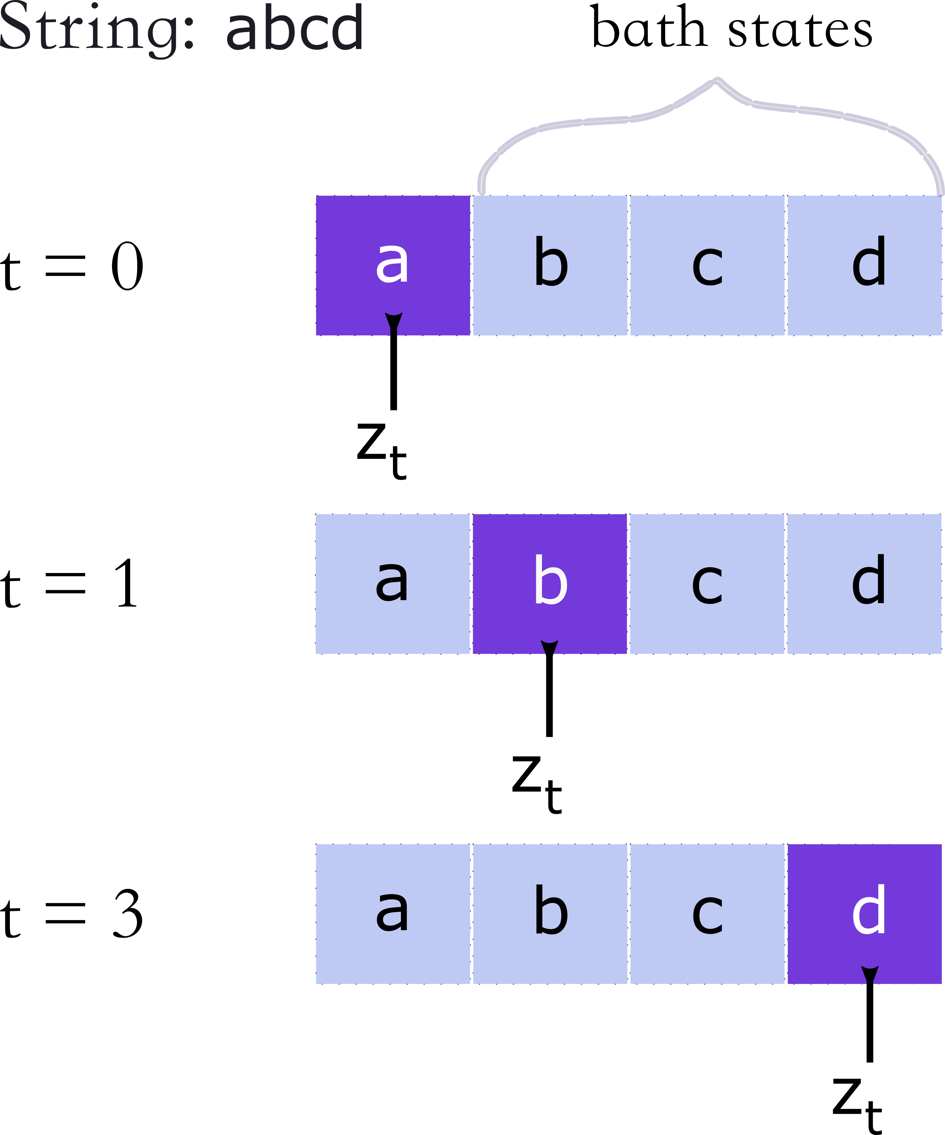
The time evolution of bath states in the bilateral decomposition is shown in Fig. 4. Just as with the unilateral decomposition, the second desideratum is automatically satisfied for the bilateral decomposition so long as we choose an appropriate initial distribution over the set of triples $(s,z,\omega)$.

There are some extra subtleties with establishing the third desideratum for the bilateral decomposition. Note that the full string $\omega$ at $t=0$ is generated as two separate substrings. The first symbol, $\omega[0]$, is one component of the SOI, and so is generated by sampling the SOI. The string of the remaining symbols, $\omega[-0]$, is the full state of the bath at $t=0$. So the full string $\omega$ is generated at $t=0$ by sampling $p_{0}(\omega[0])\rho_{0}(\omega[-0])$. The associated value of the bath Hamiltonian is $B(\omega[-0])=-\ln\rho_{0}(\omega[-0])$.

As the state of the bath at some later iteration $z=t$ will be $\omega[-z]$, we must ensure that its value under the function $B$ is nonzero for any string $\omega$ that can occur with nonzero probability. In other words, it must be the case that for all $\omega\in\rm{supp}\left[p_{0}(\omega[0])\rho_{0}(\omega[-0])\right]$, for all $t$, $B(\omega[-z])$ is finite. This condition requires in turn that $p_{0}(\omega[0])\rho_{0}(\omega[-z])$ is also nonzero for that string $\omega$. In general, whether this condition is met will depend on the details of the update function of the DFA, as well as the precise distributions $p_{0}$ and $\rho_{0}$. However, this condition is always met if both $p_{0}$ and $\rho_{0}$ have full support, since that ensures that every $\omega$ has nonzero probability of being generated at $t=0$. In such a case, the third desideratum is automatically satisfied for the bilateral decomposition.

Figure 4: Recall that states of the baths are encoded as binary strings. In bilateral decomposition, in going from $t=0$ to $t=1$, the bath state changes from $\mathrm{bcd}$ to $\mathrm{acd}$.

V Inclusive thermodynamics of DFAs

In this section, we build on the inclusive formulation of the dynamics of physical computers which implement DFAs discussed just above, to introduce the inclusive thermodynamics of logical computers.

First, in Section V.1, we derive the expression for the REP, i.e., we derive a lower bound on the expected dissipated work during the reinitialization. Next, in Section V.2.1 we show how to formulate Markov information sources (also known as HMMs or probabilistic DFAs), and in Section V.2.2 we provide exact expressions for the expected EP incurred in the computational cycle of a Markov source. Building on these analyses in Section V.2, in the following subsections we present our IFT and mismatch cost result for the forward dynamics of logical computers which are modeled by the inclusive formulation. After that, in Section V.6 and Section V.7 we extend the formulation of Markov sources to include multiple baths, and show how to interpret such systems as models of communication channels. Next we consider systems with multiple baths and derive a modified XFT which applies to not only our inclusive formulation of communication channels, but also to finite systems coupled to multiple finite baths as in Hamiltonian formulation.

Finally in Section V.9.1, we review some classical results from set theory, relevant to DFAs. Then in Section V.9.2, we combine those results with our expression for EP in Section V.1, to prove that for any regular language $L$, the DFA in $\Omega(L)$ which has minimal EP is the one with minimal size complexity. Our proof holds for all decompositions that satisfy the desiderata in Section IV.1, for all dynamics, and for all iterations.

V.1 Derivation of the expression for REP

In general, reinitizaliation of a physical computer involves a set of physically decoupled processes. The first of these processes reinitializes the accessible degrees of freedom of the SOI. The other processes reinitialize the separate baths. (Since we are for now focusing on the case of one bath, we will have a total of two processes.)

We do not make any assumptions for how the engineer reinitializes the accessible degrees of freedom. Because they can control these degrees of freedom, it’s even conceivable that they could use the optimal thermodynamic protocol, involving a conventional, infinite external heat reservoir with $k_{B}T=1$ to perform this reinitialization. Therefore we can only lower-bound the amount of work they need to expend in that reinitialization, by the amount that would be needed under that optimal thermodynamic protocol. Since we assume a uniform Hamiltonian over the states of the SOI, this minimal amount of work is given by the generalized Landauer bound [10, 41], as the change in the expected Shannon entropy of the SOI variables between the beginning and end of the reinitialization of the SOI:

$$\Delta H=[H(p_{t}(u))-H(p_{0}(u))]$$ (9)

We know that the engineer needs to expend work in reinitializing the SOI, since the ending distribution of that reinitialization is a delta function. However, in general they might be able to recover some work when they reinitialize the inaccessible degrees of freedom in the bath. As the engineer has no direct control over how those inaccessible degrees of freedom are reinitialized, we adopt the ansatz that the amount of work which they can recover is upper-bounded, by the amount of heat that would flow into a conventional, infinite thermal reservoir with $k_{B}T=1$, if the inaccessible degrees of freedom freely relaxed to the Boltzmann distribution of the Hamiltonian $B$ while coupled to that reservoir. Since energy is conserved under free relaxation, this heat flow is just the change in the expected energy of the inaccessible degrees of freedom:

$$\bar{Q}=[\mathbb{E}_{\rho_{0}}(B(v))-\mathbb{E}_{\rho_{t}}(B(v))]$$ (10)

The dissipated work incurred in the reinitialization of the physical computer is given by the difference between the amount of work spent on the SOI during that reinitialization, and the amount of work that can be recovered from the bath(s) during that reinitialization. A lower bound on this dissipated work is given by our lower bound on the amount of work that must be spent on the SOI, and the upper bound on the amount of work that can be extracted from the bath. Hence, the dissipated work is lower-bounded by

$$\overline{\sigma}=\Delta H-\bar{Q}$$ (11)

As mentioned, we call $\overline{\sigma}$ the reinitialization EP (REP). $\bar{Q}$ in Eq. 12 is called the expected entropy flow (EF) in the Hamiltonian framework. We will adopt the same terminology here.

As an example, in the unilateral decomposition of a DFA, since the state of the bath does not change during the process, $\overline{Q}=0$. Therefore $\overline{\sigma}=\Delta H$. (In other words, the EP in this case equals the generalized Landauer cost of the SOI, i.e., the minimal EF that could occur under the CTMC-based version of ST.) So in particular, if the initial distribution of the SOI is a delta function — as is the case for example in a DFA — then the expression for the EP simplifies further, to $\overline{\sigma}=H(\rho_{t})$.

Eq. 11 was motivated in [29] through different physical considerations, identifying $\overline{\sigma}$ as the expected entropy production of the forward process, without any consideration of reinitialization. (We refer the reader to Appendix A for a short review of that argument in [29].) The analysis in that paper can be adapted to show that in the general case where there are $N$ baths, which are reinitialized separately of one another, in independent processes, Eq. 11 can be also written as

$$\overline{\sigma}=I(p_{t};\rho_{t}^{1};\dots;\rho_{t}^{N})+\sum_{i=1}^{N}D\left[\rho_{t}^{i}\|\rho_{0}{{}^{i}}\right]$$ (12)

where the first term on RHS is the multi-information between the SOI and all the baths at time $t$, and the second term is the sum of KL divergences between the initial time $t=0$ distribution and the ending time distribution for each bath [61].

V.2 Inclusive thermodynamics of Markov sources

In this section, we present some preliminary results concerning the thermodynamics of Markov information sources. We start in Section V.2.1 by showing how to formulate Markov sources in terms of DFAs. Subsequently in Section V.2.2 we discuss the thermodynamic implications of modeling Markov sources as in Section V.2.1.

V.2.1 Coding efficiency and Markov sources

Recall that in a standard DFA, at each iteration $t$ the DFA is currently in some associated state $s_{t}$, and then receives some symbol $\omega[t]$ to determine the next state $s_{t+1}$, as specified by its update function $f$.

In the standard interpretation of DFAs, we view each such transition-specific symbol $\omega[t]$ as being received by the DFA, and causing the DFA to implement that transition (due to the update function of the DFA). We can just as well view the exact same process as one in which the DFA is currently in state $s_{t}$, and then generates a symbol $y_{t}=\omega[t]$, as it makes the (stochastic) transition from $s_{t}$ to $s_{t+1}$.

Now restrict attention to the case where there is a conditional distribution $\pi(y|s)$ defined at every state of the DFA, and the the strings $\omega$ of the DFA are generated by first sampling a distribution $\mathrm{P}(|\omega|)$ to generate a length of a string, and then running the process given in Algorithm a total of $|\omega|$ times, to generate an associated sequence of symbols from $\Sigma$. This gives us a distribution $\mathrm{P}(\omega)$.

Next, recall from Section III that a Markov source is an HMM, which at each iteration $t$ generates a symbol $y\in{\mathcal{Y}}$ by sampling a distribution that depends on the current state of the hidden variable. Each successive symbol $y$ produced in this stochastic process specifies a state transition map over the set of hidden states, $\left(m\rightarrow m^{\prime}\right)$. Furthermore, any transition between hidden states allowed by the HMM’s adjacency matrix, $\left(m\rightarrow m^{\prime}\right)$, is specified by a unique symbol $y\in\mathcal{Y}$.

This establishes that we can view the pseudo-code showing how to generate strings with Markov sources as an HMM,

for ( $i=1;\ |\omega|;\ i++$ ) $\{$

      Sample $\pi(y[i]\mid s[i-1])$ to get $y[i]$;

      Set $s[i]=f(s[i-1],i-1,y[i])$

      $\}$

where the states $s$ of the DFA are reinterpreted as hidden states $m$ of an HMM, and we identify the set of symbols that the HMM can generate, $\cal{Y}$, as the alphabet of the associated DFA $\Sigma$. Note that an important special case is where $\pi(y\mid s)$ is independent of $s$ for all iterations, so that the distribution over strings is given by IID sampling a fixed distribution. More precisely, when $\omega=\left(\omega_{t}\right)_{t\geq 1}$ is a sequence of $\Sigma$-valued IID random variables, the successively visited states over the DFA obtained by processing $\omega$ gives a first-order homogeneous Markov chain [62]. In general though, $\pi(y|s)$ is dependent on $s$ and the Markov source induces an HMM over the DFA states.

Now suppose that the symbol $y_{t}$ generated at iteration $t$ of the HMM is first encoded according to a codebook, and then sent through a lossless channel to a receiver. Also assume that the receiver knows the mapping rules associating each hidden state transition with a unique symbol. The receiver decodes the output of the channel to reconstruct $y_{t}$. If the receiver knows the previous hidden state $s_{t-1}$ at iteration $t$ (i.e., they know the previous state of the DFA), then once they reconstruct $y_{t}$, they know the current state, $s_{t}$, exactly. By induction, this means that (assuming they know the initial state of the DFA) they will always know what state $s_{t-1}$ was upon reconstructing $y_{t}$.

Without loss of generality, assume that the codebook is a separate prefix-free code for each state $s$ of the DFA. Hence the codeword lengths for the code used in the DFA state $s$ must satisfy the Kraft inequality $\sum_{y}2^{-l(y,s)}\leq 1$, where $l(y,s)$ gives the length of the associated prefix-free code for symbols $y$, parameterized by the state $s$. The minimum expected codeword length $\bar{L}_{\min}(s)$ for each such $s$-parameterized code generated by the information source at each iteration $t$ satisfies [63]:

$$H(Y_{t}\mid S_{t-1})\leq\bar{L}^{t}_{\min}(S)<H(Y_{t}\mid S_{t-1})+1$$ (13)

where

$$H(Y_{t}\mid S_{t-1})=-\sum_{s_{t-1}\in\mathcal{S}}\sum_{y_{t}\in\mathcal{Y}}P(s_{t-1})\pi(y_{t}\mid s_{t-1})\log\pi(y_{t}\mid s_{t-1})$$ (14)

and $\pi(y|s)$ is the conditional distribution of symbols $y$ generated by the HMM at state $s$.

V.2.2 Thermodynamic interpretation of Markov sources

As we emphasized in Section V.2.1, for the bilateral decomposition of Markov sources there are two cases of interest: the simpler case considers $\pi(y|s)$ being independent of $s$ at all iterations, while the more general case considers $\pi(y|s)$ being dependent on $s$. Here, for both of those cases, we provide the exact expressions for the expected EP incurred in a computational cycle of a Markov source.

First, we express the EP incurred in the time interval $[0,\tau]$ as

$$\begin{split}\overline{\sigma}&=\Delta H(S,Y,Z)-\bar{Q}\\ &=\Delta H(S,Y)+\Delta H(Z|S,Y)-\bar{Q}\end{split}$$ (15)

Because $z$ is a deterministic variable, $\Delta H(Z|S,Y)=H_{\tau}(Z|S,Y)-H_{0}(Z|S,Y)]$ is zero. In addition, since $s$ is fixed at $t=0$, we can rewrite the above equation as

$$\begin{split}\overline{\sigma}&=H_{\tau}(S,Y)-H_{0}(Y)-\bar{Q}\\ &=H_{\tau}(S|Y)+H_{\tau}(Y)-H_{0}(Y)-\bar{Q}\end{split}$$ (16)

Similarly, we can write for the EP

$$\overline{\sigma}=H_{\tau}(Y|S)+H_{\tau}(S)-H_{0}(Y)-\bar{Q}$$ (17)

These are our first two results concerning the thermodynamics of DFA-based Markov sources.

Note that for any given DFA modeled under the unilateral decomposition, the three quantities $H_{\tau}(Y),H_{0}(Y),$ and $\bar{Q}$ only depend on the distribution over strings. In particular, they are independent of the number of states of the DFA, or its update function. However, given that we define Markov sources in terms of $\pi(y|s)$, changes to the update function for a fixed $\pi(y|s)$ results in changes to all three of those quantities, in general.

Now, consider the first case we mentioned above, where $\pi(y|s)$ is chosen to be independent of $s$. Then those three quantities are independent of all details of the DFA. So for this situation, we can easily compare any two DFAs, $A$ and $B$, based on their EP values incurred in a computational cycle using the same $\pi(y)$. Using Eq. 16, the difference in their EPs is given by

$$H^{A}_{\tau}(S|Y)-H^{B}_{\tau}(S|Y)$$ (18)

This has a simple information-theoretic description: it is the difference in how much information the ending symbol provides about the associated state of the hidden variable for the two associated HMMs.

In the second case considered above, regardless of $\pi$, using the equation for EP from Eq. 17 we can write

$$\overline{\sigma}=\bar{L}^{\tau}_{\min}(S)+H_{\tau}(S)-\bar{Q}$$ (19)

In particular, given any two HMMs generated with the same $\pi(y|s)$, $A$ and $B$, the difference in their EPs is

$$\bar{L}^{A}_{\min}(S)-\bar{L}^{B}_{\min}(S)+H_{\tau}^{A}(S)-H_{\tau}^{B}(S)$$ (20)

(where $\tau$ is implicit.) This gives a succinct relation between the thermodynamic cost of executing Markov sources with respect to a codebook: In going from one HMM to another, the EP changes by the sum of the associated change in minimal expected codeword length plus the associated change in the entropy of the ending distribution over hidden states.

V.3 The integral fluctuation theorem for forward dynamics of computational machines

Recall that the state of the full computational system is written as $x\in X$, and we consider its values at integer-valued times, $x_{0},x_{1},\ldots,x_{\tau}$. We write that entire trajectory of $\tau+1$ successive values of $x$ as ${\pmb{x}}$. Formally, this is what we refer to as a forward trajectory, to distinguish it from the dynamics when the computational system gets reinitialized. We will decompose that trajectory into a trajectory of the SOI, ${\pmb{u}}$, together with the trajectory of the bath, ${\pmb{v}}$. (When there are multiple baths, we have multiple such bath trajectories, indicated as ${\pmb{v}}_{i}$.)

Since the Hamiltonian framework is a topic of broad interest in the literature, in this section we derive an IFT constraining the distribution of the values $\sigma({\pmb{x}})$, the EP of the forward process that is the central concern in the inclusive Hamiltonian framework. While our approach applies more generally, we focus on forward processes that implement the dynamics of DFA.

Recall that the the main focus of the Hamiltonian framework is the thermodynamics of forward trajectories (where one also imposes some assumptions concerning the Hamiltonian of the full system that are not necessary here). Accordingly, here we will use the terminology adopted in both the classical physics version of the Hamiltonian framework [8, 64, 65] as well as the quantum-mechanical version of the Hamiltonian framework (sometimes referred to as the thermodynamics of “open systems” [66, 67]).

To begin, we define the trajectory-level EP as

$$\sigma({\pmb{x}}):=\left[\ln p_{0}(u_{0})-\ln p_{\tau}(u_{\tau})\right]-\left[B(v_{0})-B(v_{\tau})\right]$$ (21)

The expectation of $\sigma({\pmb{x}})$ over all trajectories ${\pmb{x}}$ is just $\overline{\sigma}$, the expected EP during the reinitialization process. Similarly, the expectation of the entropy flow $Q=\left[B(v_{0})-B(v_{\tau})\right]$ over all trajectories is the expected EF $\bar{Q}$ occurring in the reinitialization process (see Eq. 11).

In addition though, assuming an appropriate joint Hamiltonian over the state of the SOI and the bath, the quantity on the RHS of Eq. 21 can be motivated without any presumption of a reinitialization process, as the expected entropy production that arises in the forward process. (Indeed, showing that this quantity can be identified with the expected EP in the forward process is one of the major results of the Hamiltonian framework [29, 28].)

Note also that the distribution of values $\sigma$ is the distribution of values of forward process EP that would arise in repeated sampling of the forward process. For the reasons just given, we know that those two distributions over EP result in the same value of expected EP. In general though, the distribution of values of EP generated during the forward process differs from the distribution of values of EP that would arise by reinitialization.

V.3.1 Time-reversed processes

Here we introduce a few more concepts useful for deriving the IFT for the EP incurred during the forward computational process for a full system consisting of an SOI and a single bath. These concepts and our derivation can be easily generalized to include multiple baths.

Recall that for any decomposition of computational systems, where $\mathrm{U}$ is the SOI and $\mathrm{V}$ is the bath, we stipulate that the initial distribution over $\mathrm{U}\bm{\times}\mathrm{V}$ is a product distribution, and write ${P}_{0}(s,z,\omega)={p}_{0}{\rho}_{0}$. Also recall that we require the support of ${P}_{0}$ to be restricted to legal triples in any decomposition. Note that for many decompositions, the state of the bath $\mathrm{V}$ changes from one iteration $t$ to the next. Hence, as the SOI and the bath dynamically evolve, we must ensure that there is zero probability of $B(v_{t})$ ever being infinite for accessible regions of the state space of the bath. (Recall the third desideratum in Section IV.1.)

We define the reverse process in two steps. First, the distribution over states of the bath at the beginning of the reverse process is given by $\rho_{0}$, the same distribution that is set at beginning of the forward process. After this distribution is sampled, the reverse process is generated by running the forward process backwards in time. Using the formulation introduced in Section IV, this means that reverse processes over DFAs are obtained by iterating $\Phi^{-1}$ starting from the ending state of corresponding forward processes.

For any forward trajectory ${\pmb{x}}$, we write the reverse of that trajectory as $\tilde{{\pmb{x}}}$. The initial distribution of the reverse process and the dynamics of the reverse process provides a distribution over the entire set of reverse trajectories, which we write as $R(\tilde{{\pmb{x}}})$. We indicate marginalizations of that distribution in the usual way. In particular, given a forward trajectory ${\pmb{x}}$ going from $(q_{0},z_{0},\omega_{0})$ to $(s_{\tau},z_{\tau},\omega_{\tau})$ the probability $R(.)$ of the initial and final points in the associated reversed trajectory $\tilde{{\pmb{x}}}$ evolving from $\tilde{{\pmb{x}}}_{\tau}$ to $\tilde{{\pmb{x}}}_{0}$ is

$$R(\tilde{{\pmb{x}}}_{\tau},\tilde{{\pmb{x}}}_{0})=R((s_{\tau},z_{\tau},\omega_{\tau}),(q_{0},z_{0},\omega_{0}))$$ (22)

Using this notation, the conditional distribution

$$R(\tilde{{\pmb{x}}}_{0}=(q_{0},z_{0},\omega_{0})\,|\,\tilde{{\pmb{x}}}_{\tau}=(s_{\tau},\tau,\omega_{\tau}))$$ (23)

is well-defined for all triples $(s_{\tau},\tau,\omega_{\tau})$. In addition, it equals $0$ for all illegal triples $(s_{\tau},\tau,\omega_{\tau})$ unless $(q_{0},z_{0},\omega_{0})=(s_{\tau},\tau,\omega_{\tau})$.

To define the conditional distribution in Eq. 23 more formally, we introduce $F(s,z,\omega)$ (resp. its inverse, $F^{-1}$) as the joint state of the full system, obtained by applying $\Phi$ (resp. $\Phi^{-1}$) a total of $\tau$ times, starting with $(s,z,\omega)$.

Then the conditional distribution of the entire reverse trajectory, given the entire forward trajectory, can be written as

$$R(\tilde{{\pmb{x}}}_{0}\,|\,\tilde{{\pmb{x}}}_{\tau})=\delta(F^{-1}(\tilde{{\pmb{x}}}_{\tau}),\tilde{{\pmb{x}}}_{0})$$ (24)

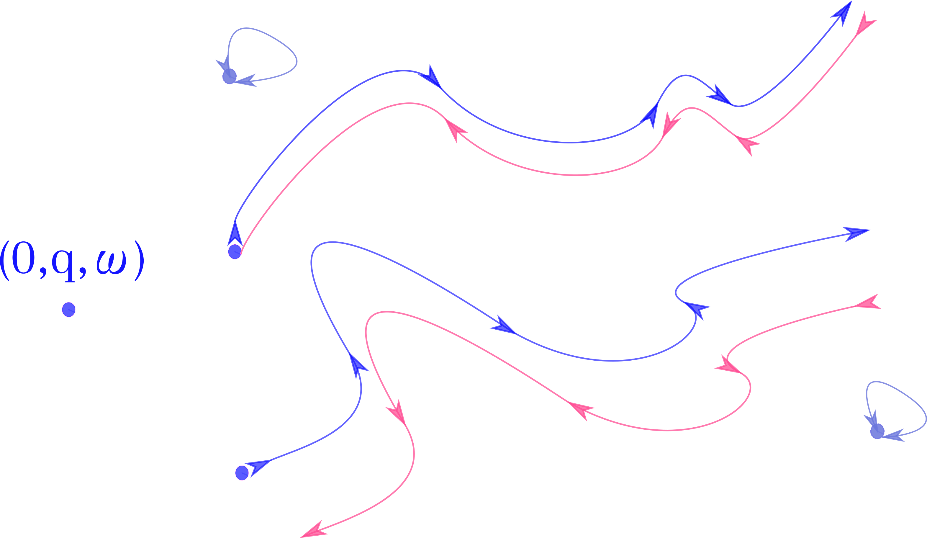
Combining the above with the specification of the initial distribution over the full system in the reverse process, where we write $R_{0}=p_{0}\rho_{0}$, we complete the definition of the reverse dynamics. A subtle point is that mostly, for the initial distribution of the reverse process to have this form of $R_{0}$, there must be nonzero probability of an initial state of the reverse process (an initial state for which $z=\tau$) that is illegal. Those triples cannot possibly arise in the forward process. As we run that reverse process, due to our definition of $\Phi$, any such illegal point can only be mapped to other illegal points, as illustrated in Fig. 5.

Figure 5: Schematical illustration of forward (in blue) reverse (in orange) trajectories, which can be defined over legal triples $\{(s,z,\omega)\}$. Illegal triples can evolve under arbitrary dynamics so long as they are only mapped to illegal triples at each iteration. The indicated dynamics is the special case where every illegal state is mapped back to itself.

V.3.2 Derivation

Suppose that we are provided a pair of (possibly vector-valued) functions $\mathrm{U}$ and $\mathrm{V}$, both defined over the space $\mathcal{T}\times S\times\Sigma^{\tau}$, such that the function $g(.,.,.)$ is a bijection. As described above, the value $u=u(s,z,\omega)$ is the state of the SOI and the value $v=v(s,z,\omega)$ is the state of the bath. We write the random variable of the trajectory of states of the SOI given by the forward process as ${\pmb{u}}=({\pmb{u}}_{0},\ldots,{\pmb{u}}_{\tau})$. A particular value of that random variable is $(u_{0},\ldots,u_{\tau})$. Similarly, we write the random variable of the trajectory of states of the SOI given by the reverse process as $\tilde{{\pmb{u}}}=(\tilde{{\pmb{u}}}_{0},\ldots,\tilde{{\pmb{u}}}_{\tau})$, where a particular value of that random variable is $(\tilde{u}_{0},\ldots,\tilde{u}_{\tau})=(u_{\tau},\ldots,u_{0})$ (Note that $\tilde{{\pmb{u}}}$ is a bijective function of ${u}$; they are not statistically independent variables in any of the equations below.) We extend this notation in the obvious way to the bath, defining the forward process random variable of the trajectory of the bath as ${\pmb{v}}=({\pmb{v}}_{0},\ldots,{\pmb{v}}_{\tau})$ with values given by vectors $(v_{0},\ldots,v_{\tau})$, and the associated reverse process trajectory as $\tilde{{\pmb{v}}}=(\tilde{{\pmb{v}}}_{0},\ldots,\tilde{{\pmb{v}}}_{\tau})$ with a particular value of that random variable written as the vector $(\tilde{v}_{0},\ldots,\tilde{v}_{\tau})=(v_{\tau},\ldots,v_{0})$.

Recall that the EF for any given forward trajectory is $Q(v_{0},v_{\tau}):=[B(v_{0})-B(v_{\tau})]$. Moreover, we can write

$$e^{Q(v_{0},v_{\tau})}=\frac{P\left(v_{\tau}\right)}{P\left(v_{0}\right)}$$ (25)

In addition,

$$Q(\tilde{v}_{0},\tilde{v}_{\tau})=Q({v}_{\tau},{v}_{0})=-Q({v}_{0},{v}_{\tau})$$ (26)

i.e., the EF generated by a reverse of a forward trajectory is the negative of the EF generated under that forward trajectory.

Given how the reverse process is defined in terms of the forward process, with the forward trajectory being $(u_{0},v_{0},u_{\tau},v_{\tau})$ and the reverse trajectory being $(u_{\tau},v_{\tau},u_{0},v_{0})$,

$$\begin{split}\frac{P(u_{0},v_{0},u_{\tau},v_{\tau})}{R(u_{\tau},v_{\tau},u_{0},v_{0})}&=\frac{P(u_{\tau},v_{\tau}|u_{0},v_{0})P(u_{0},v_{0})}{R(u_{0},v_{0}|u_{\tau},v_{\tau})R(u_{\tau},v_{\tau})}\\ &=\frac{P(u_{\tau},v_{\tau}|u_{0},v_{0})P(u_{0})P(v_{0})}{R(u_{0},v_{0}|u_{\tau},v_{\tau})R(u_{\tau})R(v_{\tau})}\\ &=\frac{P(u_{\tau},v_{\tau}|u_{0},v_{0})P(u_{0})P(v_{0})}{R(u_{0},v_{0}|u_{\tau},v_{\tau}){P}(u_{\tau})R(v_{\tau})}\\ &=\frac{e^{[\ln P_{0}(u_{0})]-B(v_{0})}}{e^{[\ln P(u_{\tau})]-B(v_{\tau})}}\\ &=e^{\sigma(u_{0},v_{0},u_{\tau},v_{\tau})}\end{split}$$ (27)

Next, as in the usual way of deriving an IFT from a DFT, we clear terms to write

$$e^{-\sigma(u_{0},v_{0},u_{\tau},v_{\tau})}P(u_{0},v_{0},u_{\tau},v_{\tau})=R(u_{\tau},v_{\tau},u_{0},v_{0})$$ (28)

If we now integrate both sides over those quadruples $(u_{0},v_{0},u_{\tau},v_{\tau})$ that can occur in the forward process, we get

$$\langle e^{\sigma}\rangle=1-\kappa$$ (29)

In this equation, $\kappa$ is the probability of generating a trajectory $(u_{\tau},v_{\tau},u_{0},v_{0})$ under the reverse process such that the forward version of that trajectory, $(u_{0},v_{0},u_{\tau},v_{\tau})$, cannot be realized under the forward process, due to the restriction that the SOI start in its initialized state . So the RHS of the IFT is not $1$ but rather less than $1$ because the support of the joint distribution at $t=0$ is less than the full joint space.

V.4 Mismatch costs for forward dynamics of computational machines

Note that no matter how a given DFA is implemented as a physical system, in general it can be initialized with an arbitrary initial distribution $p_{0}$. In this section, we analyze how changes to that initial distribution of a fixed physical system implementing a DFA affects the EP that is generated in any forward process of the computational cycle of the DFA .

Consider a physical system evolving from time $t_{0}=0$ to $t_{f}=\tau$ in a fixed physical process. In general, as we vary the distribution over the states of the system at $t_{0}$, we change the total EP generated in the (fixed) physical process. Let $\alpha_{t_{0}}$ be the distribution which results in minimal EP of that fixed physical process,

$$\alpha_{t_{0}}:=\underset{p_{t_{0}}}{\arg\min}\overline{\sigma}\left(p_{t_{0}}\right)$$ (30)

Following earlier terminology in the literature, we refer to $\alpha_{t_{0}}$ as the prior distribution for the process. While $\alpha_{t_{0}}$ is an initial distribution that results in minimal EP, in general the process might begin with a different initial distribution $\beta_{t_{0}}$, resulting in a mismatch cost $\mathcal{W}$, defined as the extra EP due to using a non-optimal intial distribution, $\mathcal{W}=\overline{\sigma}\left(\beta_{t_{0}}\right)-\overline{\sigma}\left(\alpha_{t_{0}}\right)\geqslant 0$ [51, 41].

The main result of [51] is that for a system evolving under a CTMC from $t_{0}$ to $\tau$, $\mathcal{W}$ is the change from $t_{0}$ to $\tau$ of the KL divergences between $\alpha_{t}$ and $\beta_{t}$:

$$\mathcal{W}=D\left(\beta_{t_{0}}\|\alpha_{t_{0}}\right)-D\left(\beta_{\tau}\|\alpha_{\tau}\right)$$ (31)

This result was extended in [70, 65] to apply to Langevin dynamics and to open quantum systems evolving in continuous time. In addition, fluctuation theorems for mismatch cost were derived in those papers, as were differential formulas for the instantaneous dynamics of mismatch cost.

Recall that in [70] we calculated the dissipated work incurred in the reinitialization process of the computational system using the CTMC-based approach to stochastic thermodynamics. Therefore we can use Eq. 31 to calculate the mismatch cost of that reinitialization, getting

$$\mathcal{W}_{reinit}=D\left(P_{\tau}(U,V)\|\alpha_{\tau}\right)-D\left(P_{t_{0}}(U,V)\|\alpha_{t_{0}}\right)$$ (32)

where $\alpha_{\tau}$ is the joint distribution over $U\times V$ at time $\tau$ that would result in minimal EP in the reinitialization, and $\alpha_{t_{0}}$ is the form that distribution takes after evolving according to the reinitialization process described in LABEL:PhysRevE.104.054107.

However, we cannot apply Eq. 31 to analyze the mismatch cost of the forward process, since unlike the reinitialization process, it is based on the inclusive Hamiltonian approach, not the CTMC-based approach. In this section we fill in this gap in the literature, by proving that Eq. 31 also applies in an inclusive Hamiltonian setting, even when the stopping time $\tau$ is a random variable .

The derivations of Eq. 31 in earlier analyses were based on how the change in nonequilibrium free energy of the SOI from the beginning to the end of the process gets modified if the initial distribution only is changed, with the thermodynamic process itself not changing. These nonequilibrium free energies are defined as the difference between the entropy of the SOI and the expected energy of the SOI. In the inclusive Hamiltonian framework though, the EP is defined in terms of the difference between the entropy of the SOI and the expected energy of the bath, and so requires a different analysis.

To begin this analysis, for simplicity we presume that $\alpha_{0}$ has full support, i.e., it is in the interior of the unit simplex . Under this assumption, for any initial state distribution $\beta_{t_{0}}$, the directional derivative at $\alpha_{t_{0}}$ obeys

$$\left(\beta_{0}-\alpha_{0}\right)\cdot\nabla\overline{\sigma}\left(p_{0}\right)|_{p_{0}=\alpha_{0}}=0$$ (33)

where the gradient is with respect to the components of the distribution $p_{0}$.

Note that the term $\nabla\overline{\sigma}\left(p_{0}\right)|_{p_{0}}=\alpha_{0}$ in Eq. 33 is not restricted to lie in the unit simplex in general, i.e., it can point in a direction that results in probabilities that are not normalized. Plugging in from Eq. 11, that gradient is

$$\nabla\overline{\sigma}\left(p_{0}\right)|_{p_{0}}=\nabla\Delta H\left(p_{0}\right)|_{p_{0}}-\nabla\bar{Q}\left(p_{0}\right)|_{p_{0}}$$ (34)

Consider the second gradient in Eq. 34. Component $u_{0}$ of that gradient is

$$\frac{\partial\bar{Q}(p_{0},\rho_{0})}{\partial p_{0}(u_{0})} =\frac{\partial}{\partial p_{0}(u_{0})}\left(\sum_{v}\rho_{\tau}(v)B(v)-\sum_{v}\rho_{0}(v)B(v)\right)$$ (35)

While $\rho_{0}(v)$ is independent of $p_{0}(u_{0})$ for all states $v$, that is not true of $\rho_{t}(v)$ in general, due to interactions between the SOI and the bath during the interval $[0,\tau]$. So Eq. 35 reduces to

$$\frac{\partial\bar{Q}(p_{0},\rho_{0})}{\partial p_{0}(u_{0})} =\frac{\partial}{\partial p_{0}(u_{0})}\sum_{u_{\tau},v_{\tau}}P_{\tau}(u_{\tau},v_{\tau})B(v_{\tau})$$ (36)

where $P_{\tau}(u_{\tau},v_{\tau})$ is the distribution at $t=\tau$ over the joint states of the full system. Since at $t=0$ the joint distribution is a product distribution, we can expand $P_{\tau}(u_{\tau},v_{\tau})$ as

$$p_{0}\left[F^{-1}_{U}(u_{\tau},v_{\tau})\right]\rho_{0}\left[F^{-1}_{V}(u_{\tau},v_{\tau})\right]$$ (37)

where as before, $F^{-1}(u_{\tau},v_{\tau})$ is the inverse dynamics function taking the final state $(u_{\tau},v_{\tau})$ to the (unique) associated initial state, $(u_{0},v_{0})$, with $F^{-1}_{U}(u_{\tau},v_{\tau})$ being that associated $u_{0}$ and $F^{-1}_{V}(u_{\tau},v_{\tau})$ being the associated $v_{0}$. Plugging in,

$$\begin{split}\frac{\partial\bar{Q}(p_{0},\rho_{0})}{\partial p_{0}(u_{0})}&=\sum_{u_{\tau},v_{\tau}}B(v_{\tau})\rho_{0}\left[F^{-1}_{V}(u_{\tau},v_{\tau})\right]\frac{\partial p_{0}\left[F^{-1}_{U}(u_{\tau},v_{\tau})\right]}{\partial p_{0}(u_{0})}\\ &=\sum_{u_{\tau},v_{\tau}}B(v_{\tau})\rho_{0}\left[F^{-1}_{V}(u_{\tau},v_{\tau})\right]\delta(u_{0},F^{-1}_{U}(u_{\tau},v_{\tau}))\\ &:=Q(u_{0})\end{split}$$ (38)

$Q(u_{0})$ depends on $u_{0}$ but is independent of the associated value $p_{0}(u_{0})$. Since this is true for all $u_{0}$, we can write $\bar{Q}(p_{0},\rho_{0})=\sum_{u_{0}}p_{0}(u_{0})Q(u_{0})$, i.e., the change in the expected heat of the bath is a linear function of the initial distribution over states of the SOI.

We can combine Eq. 34 with this result to evaluate the components of $\nabla\overline{\sigma}\left(p_{0}\right)$:

$$\begin{split}\frac{\partial{\overline{\sigma}\left(p_{0}\right)}}{\partial p_{0}\left(u_{0}\right)}&=\left[-\sum_{u_{\tau}}p\left(u_{\tau}\mid u_{0}\right)\ln\left(\sum_{u_{0}^{\prime}}p_{0}\left(u_{0}^{\prime}\right)p\left(u_{\tau}\mid u_{0}^{\prime}\right)\right)-1\right]\\ &\qquad+\left[\ln p\left(u_{0}\right)+1\right]-Q\left(u_{0})\right)\\ &=-\sum_{u_{\tau}}p\left(u_{\tau}\mid u_{0}\right)\ln p_{1}\left(u_{\tau}\right)+\ln p_{0}\left(v_{0}\right)-Q\left(u_{0}\right)\end{split}$$ (39)

Using equations Eq. 39 and Eq. 11, we express the inner products in the following form

$$\begin{split}\alpha_{0}\cdot\nabla\overline{\sigma}\left(\alpha_{0}\right)&=H\left(\alpha_{\tau}\right)-H\left(\alpha_{0}\right)-\bar{Q}=\overline{\sigma}\left(\alpha_{0}\right)\\ \beta_{0}\cdot\nabla\overline{\sigma}\left(\alpha_{0}\right)&=C\left(\beta_{\tau}\|\alpha_{\tau}\right)-C\left(\beta_{0}\|\alpha_{0}\right)-\bar{Q}\\ &=D\left(\beta_{\tau}\|\alpha_{\tau}\right)-D\left(\beta_{0}\|\alpha_{0}\right)+\overline{\sigma}(\beta_{0})\end{split}$$ (40)

where $C(p\|q):=-\sum_{x}p(x)\ln q(x)$ is the cross-entropy between two distributions. Combining with Eq. 33, Eq. 40 gives Eq. 31 for $\mathcal{W}$, as claimed.

There are several comments worth making. First, note that the same kind of reasoning used above not only gives the dependence of the EP on the initial distribution, but also (for appropriately redefined priors $\alpha_{t_{0}}$) gives the dependence on the initial distribution of the change in entropy of the SOI; of the non-adiabatic EP; and of the change in non-equilibrium free energy .

Second, when analyzing the thermodynamics of DFAs, it makes sense not only to consider total EP generated up to a fixed time $\tau$, but also to consider total EP generated up to either $\tau$ or the earliest time that the DFA enters an accept state, $\tau_{accept}(\mathbb{x})$, whichever comes first. In other words, when considering the thermodynamics of computational machines, we are often interested in the thermodynamics up to a stopping time that is a random variable, set by the earliest instance when a particular stopping condition (e.g., an accept state being reached) is met. This is true in particular for DFAs.

Formally, to accommodate such a random stopping time means that in defining the expected EP, we should average over values $T(\mathbb{x}):=\min[\tau,\tau_{accept}(\mathbb{x})]$, as well as average over trajectories $\mathbb{x}$. It turns out we can do this simply by fixing the update function of the DFA to never again change the state of the DFA once it enters the accept state . To see this, note that since the input string doesn’t change its state at any times, the mutual information between the SOI and the bath won’t change once the DFA enters the accept state. So with this update function, the average of EP integrated up to the random time $T(\mathbb{x})$ is equivalent to the usual integrated EP, where we always integrate up to the fixed time $\tau$.

V.5 Inclusive formulation of communication systems

In this section, we apply the inclusive formulation of DFAs to communication channels. Specifically, we extend the formulation of the bilateral decomposition for Markov sources, so that in addition to a random process representing an information source, there is a second random process representing the noise in a channel that communicates the output of that information source to a receiver. We start with Section V.6, where we formalize this extension by introducing multiple baths (e.g., a second bath provides the noise in that communication channel). We name the resulting decomposition which is suitable to model communication channels as the multilateral decomposition. In Section V.6, we also show how to expand the formalism in Section IV.3 to this decomposition. In Section V.7, we present two thermodynamically motivated distortion functions for communication channels. In Section V.8, we exploit the properties of the multilateral decomposition to derive a modified version of XFTs.

V.6 Multiple baths coordinate systems for communication channels

We start by considering a Markov information source where as above, its states are written as $s$, and each state transition at iteration $t$ generates a unique associated output symbol $y$. Recall that $\omega$ is independent of $t$, being set by sampling an appropriate distribution $\mathrm{P}_{0}(\omega)$ before the SOI starts dynamically evolving. In the bilateral decomposition of Markov sources, we used one finite bath $\mathrm{B}_{1}$ to perturb the dynamics of the SOI, as Markov sources are only associated with one random process at a time (i.e., stochastic generation of symbols as the SOI evolves). We now extend this setup by including a communication channel which takes the input strings generated a Markov source, and provides outputs under noise.

Note that communication channels are concerned with (at least) two distinct dynamical processes, first one being the generation of strings, and the second being the transfer of those strings via a noisy medium. To model communication channels, we ascribe this first process to the coupling of the SOI to bath $\mathrm{B}_{1}$, while we ascribe the latter to the coupling of the SOI to another bath to $\mathrm{B}_{2}$. The second bath manufactures the inherent noise of a communication channel, in coherence with the usual communication theory formulation.

We write $\nu$ for a string of length $\tau$, which gives the state space of the second bath $\mathrm{B}_{2}$, sampled at the beginning of the computational cycle, just as $\omega$. As in Markov sources, we interpret the transition $s_{t}\rightarrow s_{t+1}$ as a generation of an input symbol $y_{t+1}$, which then goes through a channel $\mathrm{P}(r_{t+1}\mid y_{t+1})$, producing a channel output $r_{t+1}=(\omega[z_{t}]+\nu[z_{t}])\,\mathrm{mod\,2}.$ We assume that output strings of the channel are generated according to a distribution $\mathrm{P}(\rho\mid\omega)$, which is obtained by an IID sampling of the channel, where $\rho[z_{t+1}]=r_{t+1}$ for all $t$.

This model of communication channels naturally leads to the following decomposition of the joint state space $\mathrm{U}\bm{\times}\Pi_{i}\mathrm{V}^{i}$, where we define the SOI state space over quadruples: $\mathrm{U}=\{s_{t},\omega[z_{t}],(\omega[z_{t}]+\nu[z_{t}])\,\mathrm{mod\,2},z_{t}\}$, and there are two distinct baths with state spaces $\mathrm{V}_{1}=\{\omega[-z_{t}]\}$, $\mathrm{V}_{2}=\{\nu[-z_{t}]\}$, respectively. We henceforth refer to this decomposition as the multilateral decomposition. In this decomposition, the set of elements of $\omega$ that give the state of the bath $\mathrm{B}_{1}$ change from one iteration to the next, as well as the set of elements of $\nu$. Although, as in bilateral decomposition, we do not change the definition of the bath from one iteration to the next in that decomposition. So in a similar way to Section IV.3, we provide below the bijective function $g$ for multilateral decomposition, which ensures the consistency of our approach.

Recall that $g$ maps any triple $(s,z,\omega)$ into an element of a fixed Cartesian product space $\mathrm{U}\bm{\times}\Pi_{i}\mathrm{V_{i}}$. For the multilateral decomposition, using the notation from Section IV.3, the space of the full system is given by $\mathcal{T}\times S\times\Sigma^{\tau+1}\times\Sigma_{0,1}^{\tau+1}$, where $\mathrm{U}:=\mathcal{T}\times S\times\Sigma\times\Sigma_{0,1}$, and $\mathrm{V}_{1}:=\Sigma^{\tau},$ $\mathrm{V}_{2}=\Sigma_{0,1}^{\tau}$. Here we define three associated functions $g^{U}_{ml}:\mathcal{T}\times S\times\Sigma^{\tau+1}\times\Sigma_{0,1}^{\tau+1}\rightarrow U$, $g^{V_{1}}_{ml}:\mathcal{T}\times S\times\Sigma^{\tau+1}\times\Sigma_{0,1}^{\tau+1}\rightarrow\mathrm{V}_{1},$ and $g^{V_{2}}_{ml}:\mathcal{T}\times S\times\Sigma^{\tau+1}\times\Sigma_{0,1}^{\tau+1}\rightarrow\mathrm{V}_{2}$:

$$g^{U}_{ml}(s,z,\omega,\nu) :=(s,\omega[z],\omega[z]+\nu[z]\,\mathrm{mod\,2},z)$$ (41)

$$g^{V_{1}}_{ml}(s,z,\omega,\nu) :=\omega[-z]$$ (42)

$$g^{V_{2}}_{ml}(s,z,\omega,\nu) :=\nu[-z]$$ (43)

which in turn allows us to express the dynamics over computational systems, including communication channels, which can be modeled by the multilateral decomposition.

V.7 Thermodynamic rate-distortion functions

Assume that we have a discrete source that produces a sequence of symbols $Y_{1},Y_{2},\ldots,Y_{n}$ i.i.d. $\sim p(y),y\in\mathcal{Y}$, where each $Y_{k}$ assumes values in the source alphabet $\mathcal{Y}$. We consider the distortion that results when the source produces a symbol $y$, and an associated test communication channel delivers another symbol $r$ from the alphabet $\mathcal{R}$, as its representation of $y$. In general, it is possible to express such distortion as $d\left(y_{k},r_{k}\right)$, where $d(\cdot,\cdot):\mathcal{Y}\times\mathcal{R}\rightarrow[0,\infty)$ [76].

Recall from Section III that $Q=\{Q(r\mid y),y\in\mathcal{Y},r\in\mathcal{R}\}$ formulates a communication channel. Given a source distribution $\{p(y)\}$, we associate with any such channel $Q$ two non-negative quantities $d(Q)$ and $I(Q)$ defined by

$$\begin{split}&d(Q)=\sum_{y\in\mathcal{Y}}\sum_{r\in\mathcal{R}}p(y)Q(r\mid y)d(y,r)\\ &I(Q)=\sum_{y\in\mathcal{Y}}\sum_{r\in\mathcal{R}}p(y)Q(r\mid y)\log\left(\frac{Q(r\mid y)}{q(r)}\right)\end{split}$$ (44)

where

$$q(r)=\sum_{y\in\mathcal{Y}}p(y)Q(r\mid y).$$ (45)

The quantities $d(Q)$ and $I(Q)$ are, respectively, the average distortion and the average Shannon mutual information associated with channel $Q$. The rate-distortion function of the i.i.d. source with symbol distribution $\left\{p(y)\right\}$ given the distortion constraint $d(\cdot,\cdot)$ is defined as the solution to the minimization problem:

$$R(D)=\min_{Q:d(Q)\leq D}I(Q).$$ (46)

which is solved over all conditional distributions $p(r\mid y)$ for which the joint distribution $p(y,r)=p(y)p(r\mid y)$ satisfies the expected distortion constraint.

There are many possible distortion functions; which one to consider depends on the concerns of the engineer using the communication channel. We conjecture two possible, thermodynamically motivated distortion functions including EP below.

$$\begin{split}d^{I}_{z}(y,r)&=\mathbb{E}(\sigma\mid r,z)-\mathbb{E}(\sigma\mid y,z)\\ &=\sum_{y^{\prime}}P(y^{\prime}\mid r,z)\mathbb{E}(\sigma\mid r,y^{\prime},z)\\ &\qquad-\sum_{r^{\prime}}P(r^{\prime}\mid y,z)\mathbb{E}(\sigma\mid r^{\prime},y,z)\end{split}$$ (47)

$$\begin{split}d^{II}_{z}(y,r)&=\mathbb{E}(\sigma\mid y,r,z)-\mathbb{E}(\sigma\mid y,z)\end{split}$$ (48)

(Note that so long as the state spaces of the variables in Eq. 47 and Eq. 48 are finite, we can always ensure non-negativity of those two candidate distortion functions simply by subtracting their respective minimal values.)

V.8 Modified XFTs for forward dynamics of computational machines

In the Hamiltonian framework, an XFT is a symmetry relation concerning the heat exchange incurred during a thermodynamic process including multiple finite baths that are connected with one another, and that are initially prepared at different temperatures [31, 30]. The simplest form of an XFT, for two baths, is

$$\ln\frac{p_{\tau}(+Q)}{p_{\tau}(-Q)}=\Delta\beta Q$$ (49)

where $\Delta\beta=\beta_{1}-\beta_{2}$ is the difference between the inverse temperatures at which the baths are prepared, and $Q$ is the heat flow between them during a thermodynamic process. These XFTs apply when there the baths are only connected to one another, without any SOI.

In this subsection, we show how to derive a modified version of the XFTs for the inclusive framework, in which there an SOI coupled with multiple baths, e.g., in the inclusive framework formulation of communication channels. This XFT relates the work expended on the SOI during the forward process and the net heat flow among the baths during the forward process. (There is no simple variant of the standard inclusive Hamiltonian XFT for the reinitialization process, since that process involves coupling to infinite thermal reservoirs.)

We follow [31] in how we construct an XFT, considering the case of two baths for simplicity. (The generalization to scenarios involving more than two baths is straight-forward.) Write the inverse temperatures of the two baths, $\mathrm{B}_{1}$ and $\mathrm{B}_{2}$, as $\beta_{1}$ and $\beta_{2}$, respectively. We suppose that in the forward process the two baths are coupled to the SOI via an interaction term turned on at $t=0$ and turned off at $t=\tau$. We also assume that the work performed in switching all the interaction terms (both between the baths and between each bath and the SOI) on and off can be neglected. As in our derivation of an IFT, we will also consider a reverse process that is initialized to a Boltzmann distribution.

Next, recall our assumption that the initial and final Hamiltonians of the SOI are uniform. This means that the total change in the internal energy of the SOI during the forward process is zero, and the total work $W$ done on the SOI by any infinite external work reservoir changing the Hamiltonian of the SOI is simply the sum of the total heat flow into the baths, i.e.,

$$W=\sum_{i}{Q}_{i}$$ (50)

Since both the forward process and the reverse process are initialized by sampling the respective Boltzmann distributions, the ratio of probabilities of a given forward trajectory and its reverse is

$$e^{\beta_{1}\Delta B_{1}+\beta_{2}\Delta B_{2}}$$ (51)

where the changes are evaluated at respective values at the iterations $t=0$ and $t=\tau$. Next, note that the two heat flow terms in Eq. 50 are precisely $\Delta B_{1}$ and $\Delta B_{2}$, respectively. Combining, we write the ratio of the probability of the forward trajectory to that of the reverse trajectory as

$$\frac{P({\pmb{x}}_{0})}{R(\tilde{{\pmb{x}}}_{0})}=e^{\beta_{1}Q_{1}+\beta_{2}Q_{2}}=e^{\beta_{1}Q+\beta_{2}[W-Q]}=e^{Q\Delta\beta+\beta_{2}W}$$ (52)

where $Q$ is shorthand for $Q_{1}$. Next, recall that by Eq. 26, the heat transfer during a forward trajectory is the opposite of that during the reverse of that trajectory. Combining, we write

$$\begin{split}p_{\tau}(Q)&=\int d{\pmb{x}}_{0}P({\pmb{x}}_{0})\delta(Q-Q({\pmb{x}}_{0}))\\ &=e^{Q\Delta\beta+\beta_{2}W}\int d\tilde{{\pmb{x}}}_{0}R(\tilde{{\pmb{x}}}_{0})\delta(Q+Q(\tilde{{\pmb{x}}}_{0}))\\ &=e^{Q\Delta\beta+\beta_{2}W}p_{\tau}(-Q)\end{split}$$ (53)

Note that Eq. 53 is in the form of the XFT derived by Jarzynski and Wojcik, except here we have an SOI, whose Hamiltonian might change with time.

V.9 Thermodynamic costs of computation and size complexity of DFAs

In this section, we prove that out of all DFAs which recognize the same language, the minimal complexity DFA (as defined in Section III) is the one with minimal EP at all iterations and for all dynamics.

V.9.1 Additional relevant aspects of DFAs

To proceed with our analysis, we need to first review some elementary concepts from set theory and the theory of automata. Suppose $\alpha=\left\{A_{1},A_{2},\ldots\right\}$ and $\beta=\left\{B_{1},B_{2},\ldots\right\}$ are two partitions of $\Sigma^{*}$, with blocks $A_{i}$, and $B_{j}$, respectively. We write $\alpha\preceq\beta$ if each block $B_{j}$ of $\beta$ is a union of blocks of $\alpha$, and in this case say that $\beta$ is a (partition) refinement of $\alpha$. Given two partitions $\alpha$ and $\beta$, their meet, $\alpha\wedge\beta$, (respectively, their join, $\alpha\vee\beta$ ) is the coarsest (finest) partition which refines (is refined by) both $\alpha$ and $\beta$. The meet consists of all nonempty intersections of each block of $\alpha$ with each block of $\beta$. The join consists of the smallest subsets which are a union of blocks from both $\alpha$ and $\beta$,

$$\alpha\vee\beta=\left\{A_{i}\cap B_{j}\mid A_{i}\in\alpha,B_{j}\in\beta\right\}$$ (54)

(Note that $\alpha\vee\beta=\beta$ if $\beta\preceq\alpha$.) Since any two blocks have such a meet and a join, this combination of meets and joins is a lattice, which is known as the partition lattice.

Next, recall the definition of equivalence relation $\sim_{L}$ from Section III, which provides a partition over the strings in $L$. Another equivalence relation, denoted by $\sim_{M(L)}$ (or just $\sim_{M}$ for short), is defined over the same set as $\sim_{L}$, and is specified by a particular DFA $M$ that recognizes $L$. Two strings $a,b$ are equivalent with respect to $\sim_{M}$ if processing them from the start state of $M$ puts $M$ in the same state:

$$a\sim_{M}b\Leftrightarrow f^{*}\left(q_{0},a\right)=f^{*}\left(q_{0},b\right)$$ (55)

We write the partition lattice of (the strings in) $L$ as $\Pi_{L}$ [77].

We will sometimes refer to refinements of partitions as refinements of the associated equivalence relations. More precisely, we say that the equivalence relation $\sim$ is finer than the equivalence relation $\sim^{\prime}$ if for any two $a,b\in\Sigma^{*}$

$$a\sim b\Longrightarrow a\sim^{\prime}b$$ (56)

Figure 6: Bold lines distinguish the equivalence classes of the language $L=\{\omega\mid\omega\text{ is divisible by }3\}$. $\sim_{L}$ introduces three equivalence classes over $L$, which can be bijectively mapped to the equivalence classes of $\sim_{M_{\text{min}}}$. A non-minimal DFA $M^{\prime}$ which recognizes $L$ with a larger size, as in Fig. 2, is obtained by a coarser relation $\sim_{M^{\prime}}$, whose equivalence classes are sketched by the bold and dashed lines combined.

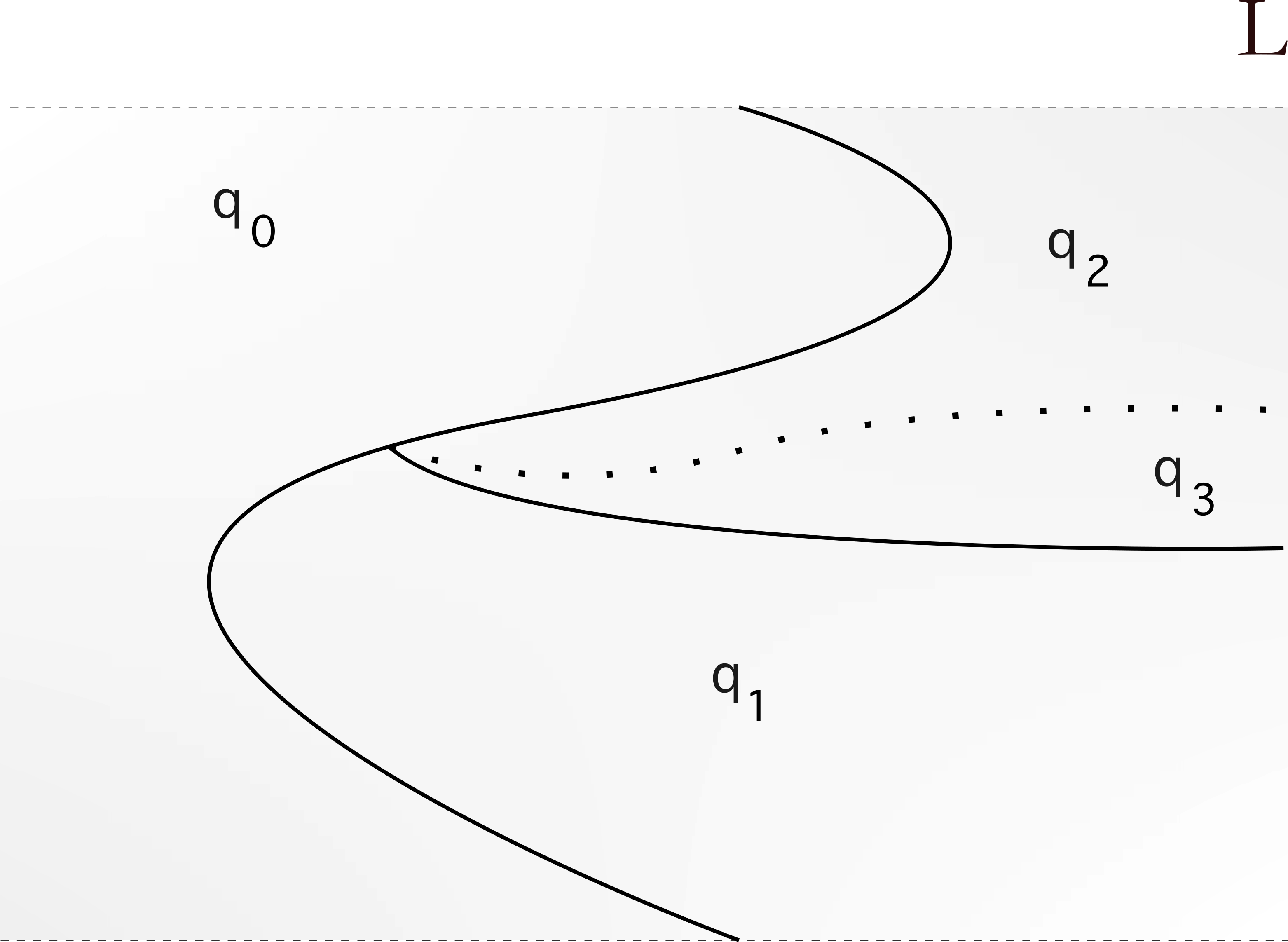
Recall that by the MN theorem, for any language $L$, the equivalence classes of $\sim_{L}$ specify a unique minimal automaton $M_{\text{min}}$. Moreover, the equivalence classes of $\sim_{M_{\text{min}}}$ (equivalently, the states of $M_{\text{min}}$) can be bijectively mapped to those of $\sim_{L}$, i.e., these equivalence classes are identical. In contrast, for any non-minimal DFA, $\sim_{M^{\prime}}$ is always coarser than both $\sim_{M}$ and $\sim_{L}$ (we illustrate this by Fig. 6).

Let $\eta$ denote the partition of $\Sigma^{*}$ corresponding to the equivalence relation $\sim_{M_{\text{min}}}$ for some regular language $L$. Any refinement $\zeta$ of $\eta$ specifies some non-minimal DFA $M^{\prime}$ which recognizes the same language $L$ that $M_{\text{min}}$ does. So the coarsest element of the lattice $\Pi_{L}$ defined above is given by the partition $\eta$. Finer elements of $\Pi_{L}$ correspond to non-minimal automata of different sizes, each formed by some refinement of $\sim_{M}$ or $\sim_{L}$. We write $H(p_{t}^{\eta})$ to express the entropy of the (probability distribution over the) equivalence classes of a minimal DFA $M_{\text{min}}$, and $H(p_{t}^{\zeta})$ to express the entropy of the (probability distribution over the) equivalence classes of a non-minimal DFA $M^{\prime}$ equivalent to $M_{\text{min}}$.

V.9.2 Minimal size complexity DFA is the one with minimal REP

In this subsection, we use the above to prove a relation between the size complexity of DFAs and the EP costs of executing DFAs.

Lemma V.1.

Under the unilateral decomposition, at all iterations $t$, for any regular language $L$, the minimal DFA for $L$ has least EP of all DFAs that recognize $L$.

Proof.

Without loss of generality, assume that any two DFAs in $\Omega(L)$ process the same set of strings sampled at time $t=0$. Since there is a bijection between the set of the states of any DFA $M$ and the equivalence classes of $\sim_{M}$, the entropy of the distribution over the states of the DFA $M$ at any iteration equals the entropy of the distribution over the equivalence class $\sim_{M}$ at that iteration. So in particular, $H(p_{t}^{\zeta})$ is the entropy at iteration $t$ of the distribution over the states of the non-minimal DFA $M^{\prime}$, and $H(p_{t}^{\eta})$ is the entropy at iteration $t$ of the distribution over the states of the minimal DFA $M_{\text{min}}$.

Next, a classic result in ergodic theory is that for any distribution over a state space, and any two partitions of that state space, $\alpha,\beta$, where $\beta$ is a refinement of $\alpha$, $H(\beta)\geq H(\alpha)$, where $H(.)$ denotes the Shannon entropy of a distribution over a partition. (Proof follows by the chain rule of entropy for partitions [78].) So in particular, $H(p_{t}^{\zeta})\geq H(p_{t}^{\eta})$. Combining establishes that at any iteration $t$

$$H_{M^{\prime}}\geq H_{M_{\text{min}}}$$ (57)

where we use $H_{M}$ as the shorthand notation for the entropy over the associated DFA states.

Next, since the dynamics of $z$ is deterministic,

$$\begin{split}H(p_{t}(s,z))&=H(p_{t}(s|z))+H(p_{t}(z))\\ &=H(p_{t}(s))\end{split}$$ (58)

for any fixed iteration $t$. So under the unilateral decomposition, the change in entropy from iteration $0$ to $t$ of the (distribution over) the states of the SOI reduces to the associated change in the entropy of the (distribution over) the state of the DFA.

Moreover, because all DFAs are initialized to a single state, $H_{t=0}=0$, and so $\Delta H_{t=\tau}=H_{t=\tau}$. Using this, we write Eq. 57 as

$$\Delta H_{M^{\prime}}\geq\Delta H_{M_{\text{min}}}$$ (59)

In the unilateral decomposition, the lower bound on the dissipated work for any DFA is given by the change in the Shannon entropy over dynamical evolution. Hence, Eq. 59 completes the proof. ∎

Lemma V.1 only concerns the unilateral decomposition. However, we can use it to derive a general result that holds for all decompositions:

Theorem V.2.

Under any decomposition, at all iterations $t$, for any regular language $L$, the minimal DFA for $L$ has least EP of all DFAs that recognize $L$.

Proof.

Without loss of generality, assume that the bath dynamics are identical for any two DFAs in $\Omega(L)$. In other words, we consider any two equivalent DFAs that process the same arbitrary set of strings being generated under some fixed dynamics. This allows us compare the dissipation costs depending only on the size complexity. Here for simplicity, we write the expected EP in the form of Eq. 12, considering one bath (although our proof can be simply generalized to multiple baths)

$$\overline{\sigma}=I\left(p_{t};\rho_{t}\right)+D\left(\rho_{t}\|\rho_{0}\right)$$ (60)

Note that the second term on the RHS is the same for any two equivalent DFAs which process the same set of strings generated by identical physical processes. However, the first term on the RHS, which gives the mutual information between the SOI and the bath at any iteration $t$, might differ for equivalent minimal and non-minimal DFAs. We express this term for a minimal and a non-minimal DFA, respectively, as follows

$$\begin{split}&I(p_{t}^{\zeta};\rho_{t})=H(\rho_{t})-H(\rho_{t}\mid p_{t}^{\zeta})\\ &I(p_{t}^{\eta};\rho_{t})=H(\rho_{t})-H(\rho_{t}\mid p_{t}^{\eta})\end{split}$$ (61)

Since conditioning cannot increase entropy, $H(\rho_{t}\mid p_{t}^{\zeta})\leq H(\rho_{t}\mid p_{t}^{\eta})$. Hence, $I(p_{t}^{\zeta};\rho_{t})\geq I(p_{t}^{\eta};\rho_{t})$. Substituting to Eq. 60 completes the proof. ∎

Recall that in conventional, CTMC-based ST, the EP given by a coarse-grained dynamics of a physical system is an upper bound on the actual EP given by the fine-grained dynamics of that system. Thus, if all we’re interested in is achieving a certain coarse-grained dynamics, the information concerning the fine-grained dynamics within each coarse-grained bin (of the phase space where dynamical evolution takes place) is redundant. Such redundancy results in extra EP without any compensating benefit for implementing the desired coarse-grained dynamics [79].

This line of reasoning does not apply directly in the inclusive framework, since the physical system implementing a minimal DFA will not be a coarse-grained version of a physical system implementing a non-minimal DFA that recognizes the same language, in general. However Theorem V.2 provides an analogous result. The partition over the set of all strings processed by a non-minimal DFA is finer-grained than it needs to be. Essentially, to avoid extra EP, it suffices to implement the same computation with a DFA whose partition would give a minimal number of bins, while retaining the needed information about the actual dynamics. For all regular languages, this is given by the minimal DFA. What Theorem V.2 shows is that the EP of that minimal DFA is the least that’s possible.

VI Related literature

There is a lot of previous research at the intersection of statistical physics and CS which focuses on using the formal tools that have been developed for analyzing systems that are in a local thermal equilibrium and applying those tools to questions in CS [80]. One example of this work is the use of the replica method to analyze neural nets [81]. Another is the use of spin glass models and associated phenomena like phase transitions to investigate computational complexity questions [82, 80, 83].

This previous research does not concern the energetic costs of real physical systems that perform computation, which is the focus of the research presented in this paper. There has already been some preliminary research on this issue. Most of this work on the thermodynamics of computation thus far focused on TMs. Early work mainly addressed TMs evolving under deterministic and logically reversible dynamics. More recently, [38] provided an ST analysis of general-purpose TMs performing irreversible computation. However, it is well known that even for basic calculations it is not possible to provide an a priori upper bound on the amount of tape a TM will use for any computational task [47]. (In fact, in part due to this, the CS research developed DFAs which can model real computers with finite resources [84]).

It is possible to compare the analyses of the inclusive framework to the standard ST analyses of computational machines, e.g., to those of TMs. In these standard analyses, the EP is taken to be zero. So all that can be calculated is the EF, which (under the usual uniform Hamiltonian assumption) is given by the drop in entropy from the beginning to the end of the computational cycle. That EF is equated with the minimal amount of work that needs to be applied by an engineer, for a computational system to complete a computational cycle.

Furthermore, under this standard approach, it’s not clear how to deal with systems that get streams of stochastic inputs (like a DFA), as the computational cycle unfolds, rather than getting all their inputs at once, when the system is initialized (like a TM does, as the initial string on its input tape) . Note as well that in this approach, if one re-initializes the system after a run, all of the expended work is recovered, and the physically vacuous conclusion is that there is zero work, independent of the details of the computational system.

As in the standard approach, we assume that a lower bound on the dissipated work during the forward process is zero. Unlike the standard approach though, we note that there is in general nonzero dissipated work in the re-initialization. This follows from the observation underlying our inclusive formulation, that there is always a difference between accessible and inaccessible degrees of freedom. This difference results in a strictly positive value for the minimal dissipated work that occurs in a complete cycle of a computational system. It also allows us to, e.g., derive a non-trivial IFT, whereas in the standard approaches with semi-static dynamics assumption, the distribution over EP values is a delta function about the value zero. As another generalization, we point out that prior work mostly assumed that a computational machine is implemented by a CTMC. Our inclusive framework allow the dynamics to be non-Markovian as well.

We propose that an inclusive thermodynamics of computation will offer rigorous tools to both advance theoretical research and engineer devices with enhanced performance. For instance, digital computers include hardware-implemented finite automata, and DFAs and NFAs are used to build systematic approaches for designing sequential circuits. The optimal design procedures of finite automata allow optimal or near-optimal physical circuit implementations [86]. Besides, in traditional architectures (CPU or GPU based), execution of an NFA may lead to a state space explosion leading to exponential run-time complexity. Hence, special-purpose architectures are required to run them . We expect that the relations between the structural constraints, CS-based complexity, and thermodynamic bounds on computation will yield valuable design-inputs for next generation of the processors in computers .

There might also be advantages for computers run to analyze data sets in the more general natural sciences. For instance, modern biology research uses DFAs for the characterization of protein sequences through the identification of motifs present in them. High efficiency DFAs work as an accelerator for many applications in bioinformatics and data-mining [89]. It is well-known that the computational efficiency of DFAs is encoded in the descriptional complexity of DFAs, which we showed to be related to the thermodynamic costs of physically executing DFAs.

Finally, there have been some recent papers that considered non-equilibrium thermodynamics of finite automata, using a different approach from ours [90, 91, 40]. In particular, [40] uses the CTMC version of stochastic thermodynamics, and starts by recognizing that real-world (synchronous) physical computers use a central clock to ensure that their dynamics is periodic. As a result, the prior for the dynamics at each successive iteration of such a computer is the same. However, the distribution over states of the computer will vary from one iteration to the next. Thus, there is unavoidable mismatch cost in such a computer. [40] analyzes this mismatch cost for DFAs, along with the “local” mismatch cost arising if the rate matrix governing the dynamics of the DFA’s state only has access to the current input symbol rather than the full input string. In contrast, our paper uses the inclusive Hamiltonian version of stochastic thermodynamics, and considers the full EP, not just mismatch cost. Also, we make no assumptions that the process is “periodic” or “local” in any sense.

In addition, [70] derives a formula for expected mismatch cost for the classical setting and a non-infinite bath. That is very similar to what we do here. However, [70] explicitly assumes that the SOI has a continuous-state state space, not a finite or countably infinite state space like the ones considered in this paper. In addition,  [70] explicitly states that its results hold for the Hamiltonian of mean force formulation of EP, which differs from the inclusive Hamiltonian formulation of EP considered in this paper . Finally, the results in [70] all assume that there is a fixed time $\tau$ at which the process ends, and considers all EP generated at times $t$ up to $\tau$. It does not consider the case where there is a random variable giving the time that a stopping condition is first satisfied, where the EP of interest is only the EP up to that stopping time. The results in this paper also apply to the case where the EP is integrated up to when a stopping condition is met.

VII Discussion

In this paper, we introduced a novel approach to quantify the thermodynamic costs of computation in systems operating far-from-equilibrium. In particular, we considered DFA-based computational machines, and derived a lower bound on the dissipated work that occurs in a cycle of any physical process that implements those machines. We showed that this lower bound is independent of the details of the physical process, and is formally identical to the irreversible EP arising in the Hamiltonian formulation of ST.

There are several possible directions for future work. One is to apply the inclusive framework to other computational machines in the Chomsky hierarchy, e.g., pushdown automata, or TMs. In particular, suppose we have a conventional finite cellular automaton (CA), whose initial state is determined randomly, after which is evolves in a deterministic process [93]. Such a system can be modeled as a slight variant of the unilateral decomposition of a DFA, by identifying each state of the DFA with a different state of the CA. For simplicity, suppose that the CA state is a binary string of length $k$, with the dynamics of that string given by the CA evolution rule. So the associated DFA has $2^{k}$ states. We suppose as well the bath’s state is a string of $k$ bits. At $t=-1$, the string in the bath is generated by random sampling. Then at $t=0$, the state of the DFA is set to that state of the bath, i.e., the bit string in the bath is copied into the state of the DFA / CA. After that the DFA / CA undergoes deterministic dynamics, according to the associated evolution rule of the CA. The analysis above for the inclusive thermodynamics of DFAs under the unilateral decomposition carries over almost directly, with minimal change.

Another interesting direction for future work might explore more elaborate problems in CS. For instance, a way of building computational machines that recognize more complex regular languages is to combine simple languages by using Boolean operations, and construct DFAs that recognize the composite languages obtained from the elementary ones. It is an open question whether or not there are any concise relations between thermodynamic costs concerning such composite systems and the complexity of associated language operations. Along these lines, we also hope to investigate potential connections to generative grammars [94] in the future work. Apart from that, it might be possible to translate our framework into the language of dynamical systems theory, vice versa, e.g., by considering the shift processes of DFAs [59, 95]. All in all, we anticipate that there remains much more to understand about how our thermodynamic framework can be utilized for a further exploration of (the theory of) automata and formal languages, in a way that is reminiscent of von Neumann’s notes [2].

Another open question is how the thermodynamics in the inclusive framework changes if we allow the length of the string input to the DFA to vary stochastically, and to then consider running a given DFA with a randomly set string length multiple times in succession [21].

Future work might also involve extending our mismatch cost result to performing an analysis for the mismatch cost of the reinitialization process. (Note that the reinitialization process ends with the distribution over states of the SOI being a delta function. Analyzing the mismatch cost for such a process requires the use of islands, in general.) Analogously, the IFT derived in the main text concerns the inclusive Hamiltonian definition of EP generated during the forward process. Some important future work would be to derive an IFT concerning the REP instead.

We conclude with two remarks. First, recall that reinitialization involves two parallel dynamic processes. The first is a quasi-statically slow change of a Hamiltonian of the SOI, so that the distribution of states of the SOI changes from $P_{\tau}(u_{\tau})$ back to its initialized form (which in the case of DFAs is a delta function). The SOI is in a Boltzmann distribution for its associated Hamiltonian throughout this process.

In contrast, the second process is a free relaxation of the bath under the Hamiltonian whose Boltzmann distribution is the initial distribution of the states of the bath. That relaxation takes the distribution $P_{\tau}(v_{\tau})$ to the initial distribution over bath states without any change to the Hamiltonian. The distribution of values of the EP during the reinitialization is given by subtracting the random variable of the work required in the first process from the random variable of the work extracted in the second process. In general, that distribution will differ from the distribution of values of $\sigma$, calculated above. This is true despite the fact that the expected EP in the forward process must exactly cancel the expected EP in the reinitialization process, since the sequence of reinitialization after a forward process results in the exact same distribution over states of the joint system. We refer the reader to Appendix D and Appendix E for more comments on this.

Finally, it is important to note that while DFAs and HMMs are closely related mathematically, their inclusive thermodynamic properties are quite different. Mathematically, HMMs are somewhat related to what in computer science are called “automata groups”, and are called “information ratchets in [41]. However again, this has no implications for how the inclusive thermodynamics of HMMs is related to analyses in the literature based on CTMCs for the thermodynamics of automata groups. So in particular, our HMM results do not apply to the information ratchets considered in detail in [96].

VIII Acknowledgments

David Wolpert was supported by the Santa Fe Institute and the National Science Foundation award CCF - 2221345. Gülce Kardeş thanks Matteo Marsili for stimulating discussions, and Pedro Harunari and Artemy Kolchinsky for very useful feedback on this manuscript. Gülce Kardeş acknowledges support by the Quantitative Life Sciences, International Centre for Theoretical Physics.

IX Appendices

Appendix A Expression for HEP

As in [29], consider a finite setup composed of a finite SOI and finite bath(s). Initially, at time $t=0$, the system and the baths are decoupled, $P(0)=p(0)\prod_{i}\rho_{i}^{\mathrm{eq}}$. In turn, the baths are initialized to

$$\rho_{i}(0)=\rho_{i}^{\mathrm{eq}}=\exp\left(-\beta_{i}\mathrm{H_{i}}\right)/Z_{i}$$ (62)

with $\mathrm{H_{i}}$ and $Z_{i}$ the corresponding bath Hamiltonian, and the partition function at $t=0$, respectively. The time evolution of all degrees of freedom in the joint system of the SOI and baths is governed by Hamiltonian (invertible) dynamics, with a Hamiltonian $\mathrm{H}(t)=\text{H}_{system}(t)+\sum_{i}\mathrm{H_{i}}+V(t)$. Here, $V(t)$ is an interaction term coupling the system and the baths, with the result that considered in isolation, the SOI evolves stochastically rather than deterministically.

[29] analyzes this scenario. This analysis shows that the change in the Shannon entropy of the system from the initial time $t=0$ to any later time $t>0$ can be written as $\Delta H(t)=\Delta_{i}S(t)+\Delta_{e}S(t)$, with the conventional thermodynamic interpretation of $\Delta_{e}S(t)$ as the change in expected energy of the baths divided by the associated temperatures (see Eqn. 1–7 in [29]). In our paper, we use a different notation ($\bar{\sigma}$ for $\Delta_{i}S(t)$ and $\bar{Q}$ for $\Delta_{e}S(t)$) and mainly consider classical systems. However, the decomposition of $\Delta H(t)$ in our paper is identical to that in [29]. Moreover, like the decomposition in [29], our REP result applies to both classical and quantum systems.

Appendix B EP and EF for a Markov source processing semi-infinite strings

Here, we expand the EP and EF expressions presented in Section IV for Markov sources which process semi-infinite strings (hence the state space is countably infinite).

Recall that in the bilateral decomposition of Markov sources, we identify the finite set of triples {$s,z,\omega[z]$} as the SOI state space $\mathrm{U}$, while the set of all possible {$\omega[-z]$} correspond to the bath state space $\mathrm{V}$. The bath represents the data stream which provides the subsequent symbols to be processed by the SOI. As in the main text, we write $\omega[z=t]=y$. Notably in the bilateral decomposition, the state of the bath $\omega[-z]$ changes in time, thus resulting in non-zero EF.

We formulate the expected energy of the bath at iteration $t\geq 1$ with $B(.)$ the Hamiltonian of the bath, and $\xi$ is a semi-infinite string tracked by the pointer,

$$\begin{split}\mathbb{E}(B_{t})&=\sum_{\xi_{0:\infty}}P_{t}B_{t}(\xi_{0:t-1},\xi_{t+1:\infty})\\ &=-\sum_{\xi_{0:\infty}}P_{t}\ln P(\omega_{1:t}=\xi_{0:t-1},\omega_{t+1:\infty}=\xi_{t+1:\infty})\end{split}$$ (63)

where $P_{t}=P_{t}(\omega_{0:t-1}=\xi_{0:t-1},w_{t}=\xi_{t},\omega_{t+1:\infty}=\xi_{t+1:\infty}).$ Since for general semi-infinite strings $\zeta_{1:\infty}$, we have

$$B(\zeta)=-\ln P(\omega_{1:\infty}=\zeta_{1:\infty})$$ (64)

EF for the bath at iteration $t=\tau$ can be written as

$$\bar{Q}=\mathbb{E}(B_{t=0})-\mathbb{E}(B_{t=\tau})$$ (65)

In certain scenarios we can analytically calculate EP and EF, given by these equations above. Consider for instance the Markov source which generates strings by emitting symbols drawn from a distribution $\pi(y\mid s)$, which is independent of $s$. So the change in the expected energy of the bath from $t=0$ to $t=n>0$ is

$$\bar{Q}: =\sum_{\xi_{1:n}}\ln[P(\omega_{1:n}=\xi_{1:n})]P(\omega_{1:n}=\xi_{1:n})$$ (66)

$$\quad-\sum_{\xi_{1:n}}\ln[P(\omega_{1:n}=\xi_{1:n})]P(\omega_{0:n-1}=\xi_{1:n})$$ (67)

$$=-H(P(\omega_{0}))-\sum_{i=1}^{n}H(P(\omega_{i}\mid\omega_{i-1}))$$ (68)

$$\quad-\sum_{\xi_{1:n}}\ln[P(\omega_{1:n}=\xi_{1:n})]P(\omega_{0:n-1}=\xi_{1:n})$$ (69)

Similarly, since in any iteration $t$, $z=t$ with probability $1$, the change in entropy is

$$\Delta H :=H(P(S_{n},Z_{n},\omega_{n}))-H(P(S_{0},Z_{0},\omega_{0}))$$ (70)

$$=H(P(S_{n},\omega_{n}))-H(P(\omega_{0}))$$ (71)

$$=H(P(\omega_{n}\mid S_{n}))+H(S_{n})-H(\omega_{0})$$ (72)

EP is given by combining $\Delta H$ and $\bar{Q}$.

Appendix C Inclusive formulation of a DFA with bi-infinite strings

Here, we extend the formulation in Section IV.2 to bi-infinite strings. In general, recall that the countably infinite state space of the full system is $(\{s,z,\omega\})$ where $s\in S$ is a state of the DFA, and $\omega$ is a string. As mentioned in the main text, $\omega$ need not be finite but it can also be bi-infinite, $\omega^{\mathbb{Z}}=\left\{y=\left(y_{z}\right)_{z\in\mathbb{Z}}:y_{z}\in A\right.$ for all $\left.z\in\mathbb{Z}\right\}$. Each entry in $\omega$ is still a member of a finite alphabet $\Sigma$ that includes a special blank symbol.

Processing a bi-infinite string generates a bi-infinite trajectory over DFA states $\mathcal{S}^{\mathbb{Z}}=\left\{s=\left(s_{z}\right)_{z\in\mathbb{Z}}:s_{z}\in S\right.$ for all $\left.z\in\mathbb{Z}\right\}$. This allows us to extend the formulation in Section IV by only slightly changing the definition of legal (resp. illegal) triples.

For bi-infinite strings, we say that a triple $(s,z,\omega)$ is legal if either of the following conditions is satisfied: $z\leq 0,s=q$, or $(s,z,\omega)=(z,f(s^{\prime},\omega[z]),\omega)$ for some legal triple, $(z-1,s^{\prime},\omega)$. To ensure that the support of the system is restricted to legal triples, we impose that $p(z,s)=1$ for $(z,s)=(0,q)$, i.e., $P_{0}(s,z,\omega)=0$ if either $z\neq 0$ and/or $s\neq q$.

Appendix D Interpretation of entropy production

Consider the inclusive Hamiltonian formula for EP generated between initialization at $t_{0}$ and some arbitrary $t>t_{0}$:

$$\bar{\sigma}_{t_{0},t} =I_{t}(p_{t};\rho_{t})-I_{t_{0}}(p_{0};\rho_{0})+D(\rho_{t}||\rho_{0})$$ (73)

$$=\Delta_{t_{0},t}I+D(\rho_{t}||\rho_{t_{0}})$$ (74)

The first term on the RHS in the second equation is additive over successive time intervals, i.e., for any pair of times $t_{1}<t_{2}$ both occurring after the initialization time $t_{0}$, it is true that

$$\Delta_{t_{0},t_{2}}I=\Delta_{t_{0},t_{1}}I+\Delta_{t_{1},t_{2}}I$$ (75)

So the first component of the formula for EP is additive. However, the second component is not:

$$D(\rho_{t_{2}}||\rho_{t_{0}})\neq D(\rho_{t_{2}}||\rho_{t_{1}})+D(\rho_{t_{1}}||\rho_{t_{0}})$$ (76)

Hence the entire formula for EP is not additive over time,

$$\sigma_{t_{0},t_{2}}\neq\sigma_{t_{0},t_{1}}+\sigma_{t_{1},t_{2}}$$ (77)

That is in stark contrast to the meaning of EP as dissipated work in the CTMC-based approach to stochastic thermodynamics. It means that it is not correct to identify $\sigma_{t_{0},t_{2}}-\sigma_{t_{0},t_{1}}$ as the “EP” in going from $t_{1}$ to $t_{2}$. Indeed, while the full EP from $t=t_{0}$ cannot be negative, the change in that full EP as we go from $t_{1}$ to $t_{2}$ can be negative. This would arguably violate the second law if in fact that change in EP were interpreted as conventional thermodynamic dissipated work. Another example of how problematic it would be to interpret $\sigma_{t_{1},t_{2}}$ as the EP in going from $t_{1}$ to $t_{2}$ is that it’s not clear what “mismatch cost contribution to EP in going from iteration $t_{1}$ to $t_{2}$” could mean.

As a final illustration of this phenomenon, note that there is no function whose only arguments are the distributions $P(u_{t_{1}},v_{t_{1}})$ and $P(u_{t_{2}},v_{t_{2}})$ that gives the change in EP between $t_{1}$ and $t_{2}$, $\sigma_{t_{0},t_{2}}-\sigma_{t_{0},t_{1}}$. In this sense, change in full EP between those two times differs from the full EP of either of those times individually — those two full EPs can both be calculated from just the associated two distributions. Now it would be possible to calculate $\sigma_{t_{0},t_{2}}-\sigma_{t_{0},t_{1}}$ with a function that has those two distributions as arguments along with the bath’s Hamiltonian function. But the latter is not needed as an argument for calculating just EP from $t_{0}$ to $t$, $\sigma_{t_{0},t}$, due to the assumption that the bath is in a Boltzmann distribution at $t_{0}$.

In summary, one should not interpret EP in the inclusive Hamiltonian framework as “dissipated work”, but as “dissipated work relative to the distribution at $t_{0}$. Viewed differently, the EP at time $t_{1}$ in the inclusive Hamiltonian framework is the total work that has been dissipated into the inaccessible degrees of freedom relative to the distribution at $t_{0}$ and so cannot be directly recovered at $t_{1}$. Moreover, as mentioned above, this EP — this work that has been dissipated into the inaccessible degrees of freedom — can decrease between $t_{1}$ and $t_{2}>t_{1}$. This reflects the fact that while the engineer cannot access the inaccessible degrees of freedom directly at $t_{1}$ and recover work, in the time following $t_{1}$ some of the energy that was put into these inaccessible degrees of freedom during $[t_{0},t_{1}]$ would be transferred back into the accessible degrees of freedom.

Appendix E Relations among different approaches

One of the advantages of the inclusive thermodynamics framework is that by ignoring all details of a physical process besides the computation it achieves, it helps focus on the thermodynamics properties inherent in just that computation. As an example, there is still misunderstanding among some researchers concerning the possible thermodynamic advantages of “logically reversible Turing machines”, or (logically reversible) “Toffoli circuits” [97]. These systems are used to compute logically irreversible deterministic maps $f:x\in X\rightarrow f(x)$ without requiring any work. Broadly speaking, to do this they replace the calculation of $f$ with the calculation of $g:(x\in X,0)\rightarrow(x,f(x))$, where the initial value $x$ is distributed according to some distribution over inputs, $p(x)$. Since $f$ is deterministic, the initial entropy of $(x,0)$ equals the ending entropy of $(x,f(x))$, and so the generalized Landauer cost implementing $g$ is zero. In contrast, if $f$ is logically irreversible, then the entropy of $p(x)$ is greater than the entropy of $p(f(x))$, and so the generalized Landauer cost of implementing $f$ is greater than $0$. This is interpreted to mean that implementing the reversible function $g$ is thermodynamically superior to implementing the irreversible function $f$.

Consider this scenario from the perspective of the inclusive framework however. The system implementing $g$ has an extra accessible variable which is not accessible to the system implementing $f$, a variable that must be initialized to $0$. (Formally, $f$ is a map over $X$ whereas $g$ is a map over $X^{2}$.) Therefore to “compare apples to apples”, we should give the system implementing $f$ access to that extra coordinate which is initialized to $0$, just like the system implementing $g$. Note though that the precise value of that extra coordinate at the end of the computation is irrelevant when we implement the irreversible map $f$, in contrast to the case with $g$. So we can suppose that in implementing this variant of $f$, we use the extra, initialized coordinate as an information reservoir, thermalizing it as we run the computation. Formally, we replace $f$ with the stochastic map, $f^{*}:(x\in X,0)\rightarrow(f(x),y)$, where $y$ is distributed according to an appropriate Boltzmann distribution, $P(y)$. In general, the Landauer cost of $f^{*}$ may be greater than that of $g$, equal to it — or less than it. So in this more fair comparison, where both systems being compared have access to the initialized coordinate, there is no a priori advantage to using a reversible computer rather than an irreversible one to implement $f$.

References

- Szilard [1929] L. Szilard, über die Entropieverminderung in einem thermodynamischen System bei Eingriffen intelligenter Wesen, Zeitschrift fur Physik 53, 840 (1929).
- von Neumann and Taub [1961] J. von Neumann and A. H. Taub, John von Neumann Collected Works (1961).
- Zurek [1990] W. H. Zurek, Complexity, Entropy and the Physics of Information (1990).
- Bennett [2003] C. H. Bennett, Notes on Landauer’s principle, reversible computation, and Maxwell’s Demon, Studies in History and Philosophy of Science Part B: Studies in History and Philosophy of Modern Physics 34, 501 (2003).
- Caves and Schack [1997] C. M. Caves and R. Schack, Unpredictability, information, and chaos, Complex. 3, 46–57 (1997).
- Sekimoto and ichi Sasa [1997] K. Sekimoto and S. ichi Sasa, Complementarity relation for irreversible process derived from stochastic energetics, Journal of the Physical Society of Japan 66, 3326 (1997).
- Crooks [1999] G. E. Crooks, Entropy production fluctuation theorem and the nonequilibrium work relation for free energy differences, Physical Review E 60, 2721 (1999).
- Jarzynski [1999] C. Jarzynski, Hamiltonian Derivation of a Detailed Fluctuation Theorem, Journal of Statistical Physics 98, 77 (1999).
- Peliti and Pigolotti [2021] L. Peliti and S. Pigolotti, Stochastic Thermodynamics: An Introduction (Princeton University Press, 2021).
- Esposito and den Broeck [2010] M. Esposito and C. V. den Broeck, Three detailed fluctuation theorems, Physical Review Letters 104, 10.1103/physrevlett.104.090601 (2010).
- Shiraishi et al. [2018] N. Shiraishi, K. Funo, and K. Saito, Speed limit for classical stochastic processes, Physical Review Letters 121, 10.1103/physrevlett.121.070601 (2018).
- Funo et al. [2019] K. Funo, N. Shiraishi, and K. Saito, Speed limit for open quantum systems, New Journal of Physics 21, 013006 (2019).
- Shiraishi and Saito [2019] N. Shiraishi and K. Saito, Information-Theoretical Bound of the Irreversibility in Thermal Relaxation Processes, Phys. Rev. Lett. 123, 110603 (2019).
- García-Pintos et al. [2021] L. P. García-Pintos, S. Nicholson, J. R. Green, A. del Campo, and A. V. Gorshkov, Unifying quantum and classical speed limits on observables (2021).
- Horowitz and Gingrich [2019] J. M. Horowitz and T. R. Gingrich, Thermodynamic uncertainty relations constrain non-equilibrium fluctuations, Nature Physics 16, 15 (2019).
- Liu et al. [2020] K. Liu, Z. Gong, and M. Ueda, Thermodynamic uncertainty relation for arbitrary initial states, Physical Review Letters 125, 10.1103/physrevlett.125.140602 (2020).
- Kardeş and Wolpert [2021] G. Kardeş and D. H. Wolpert, Thermodynamic uncertainty relations for multipartite processes (2021).
- Hasegawa and Vu [2019] Y. Hasegawa and T. V. Vu, Fluctuation theorem uncertainty relation, Physical Review Letters 123, 10.1103/physrevlett.123.110602 (2019).
- Barato and Seifert [2015] A. C. Barato and U. Seifert, Thermodynamic Uncertainty Relation for Biomolecular Processes, Phys. Rev. Lett. 114, 158101 (2015).
- Falasco and Esposito [2020] G. Falasco and M. Esposito, Dissipation-Time Uncertainty Relation, Phys. Rev. Lett. 125, 120604 (2020).
- Neri et al. [2017] I. Neri, E. Roldán, and F. Jülicher, Statistics of Infima and Stopping Times of Entropy Production and Applications to Active Molecular Processes, Phys. Rev. X 7, 011019 (2017).
- Manzano et al. [2021] G. Manzano, D. Subero, O. Maillet, R. Fazio, J. P. Pekola, and É . Roldán, Thermodynamics of gambling demons, Physical Review Letters 126, 10.1103/physrevlett.126.080603 (2021).
- Gingrich and Horowitz [2017] T. R. Gingrich and J. M. Horowitz, Fundamental bounds on first passage time fluctuations for currents, Physical Review Letters 119, 10.1103/physrevlett.119.170601 (2017).
- Garrahan [2017] J. P. Garrahan, Simple bounds on fluctuations and uncertainty relations for first-passage times of counting observables, Physical Review E 95, 10.1103/physreve.95.032134 (2017).
- Seifert [2012] U. Seifert, Stochastic thermodynamics, fluctuation theorems and molecular machines, Reports on Progress in Physics 75, 126001 (2012).
- Van den Broeck and Esposito [2015] C. Van den Broeck and M. Esposito, Ensemble and trajectory thermodynamics: A brief introduction, Physica A: Statistical Mechanics and its Applications 418, 6 (2015), proceedings of the 13th International Summer School on Fundamental Problems in Statistical Physics.
- Strasberg et al. [2017] P. Strasberg, G. Schaller, T. Brandes, and M. Esposito, Quantum and Information Thermodynamics: A Unifying Framework Based on Repeated Interactions, Phys. Rev. X 7, 021003 (2017).
- Ptaszyński and Esposito [2019] K. Ptaszyński and M. Esposito, Thermodynamics of Quantum Information Flows, Phys. Rev. Lett. 122, 150603 (2019).
- Esposito et al. [2010] M. Esposito, K. Lindenberg, and C. V. den Broeck, Entropy production as correlation between system and reservoir, New J. Phys. 12, 013013 (2010).
- Timpanaro et al. [2019] A. M. Timpanaro, G. Guarnieri, J. Goold, and G. T. Landi, Thermodynamic Uncertainty Relations from Exchange Fluctuation Theorems, Phys. Rev. Lett. 123, 090604 (2019).
- Jarzynski and Wójcik [2004] C. Jarzynski and D. K. Wójcik, Classical and Quantum Fluctuation Theorems for Heat Exchange, Phys. Rev. Lett. 92, 230602 (2004).
- Seifert [2016] U. Seifert, First and Second Law of Thermodynamics at Strong Coupling, Phys. Rev. Lett. 116, 020601 (2016).
- Strasberg et al. [2015] P. Strasberg, J. Cerrillo, G. Schaller, and T. Brandes, Thermodynamics of stochastic turing machines, Phys. Rev. E 92, 042104 (2015).
- Talkner and Hänggi [2020] P. Talkner and P. Hänggi, Comment on “measurability of nonequilibrium thermodynamics in terms of the hamiltonian of mean force”, Phys. Rev. E 102, 066101 (2020).
- Nielsen and Chuang [2010] M. A. Nielsen and I. L. Chuang, Quantum Computation and Quantum Information: 10th Anniversary Edition (Cambridge University Press, 2010).
- Breuer and Petruccione [2002] H. P. Breuer and F. Petruccione, The Theory of Open Quantum Systems (2002).
- Wolpert and Kolchinsky [2020] D. H. Wolpert and A. Kolchinsky, Thermodynamics of computing with circuits, New Journal of Physics 22, 063047 (2020).
- Kolchinsky and Wolpert [2020] A. Kolchinsky and D. H. Wolpert, Thermodynamic costs of turing machines, Physical Review Research 2, 10.1103/physrevresearch.2.033312 (2020).
- Parrondo et al. [2015] J. Parrondo, J. Horowitz, and T. Sagawa, Thermodynamics of information, Nature Phys 11, 131–139 (2015).
- Ouldridge and Wolpert [2022] T. E. Ouldridge and D. H. Wolpert, Thermodynamics of deterministic finite automata operating locally and periodically (2022).
- Wolpert [2019] D. H. Wolpert, The stochastic thermodynamics of computation, Journal of Physics A: Mathematical and Theoretical 52, 193001 (2019).
- Brittain et al. [2021] R. A. Brittain, N. S. Jones, and T. E. Ouldridge, What would it take to build a thermodynamically reversible Universal Turing machine? Computational and thermodynamic constraints in a molecular design (2021), arXiv:2102.03388 [cond-mat.stat-mech] .
- Freitas et al. [2021] N. Freitas, J.-C. Delvenne, and M. Esposito, Stochastic thermodynamics of nonlinear electronic circuits: A realistic framework for computing around kt, Physical Review X 11, 10.1103/physrevx.11.031064 (2021).
- Gao and Limmer [2021] C. Y. Gao and D. T. Limmer, Principles of low dissipation computing from a stochastic circuit model, Physical Review Research 3, 10.1103/physrevresearch.3.033169 (2021).
- Sheng et al. [2019] S. Sheng, T. Herpich, G. Diana, and M. Esposito, Thermodynamics of Majority-Logic Decoding in Information Erasure, Entropy 21, 10.3390/e21030284 (2019).
- Aaronson [2005] S. Aaronson, NP-complete Problems and Physical Reality, Electron. Colloquium Comput. Complex. (2005).
- Arora and Barak [2009] S. Arora and B. Barak, Computational Complexity: A Modern Approach, 1st ed. (Cambridge University Press, USA, 2009).
- Lewis and Papadimitriou [1997] H. R. Lewis and C. H. Papadimitriou, Elements of the Theory of Computation, 2nd ed. (Prentice Hall PTR, USA, 1997).
- Note [1] In the real world there will be many more types of degree of freedom of the full computational system than just “accessible” and “inaccessible”, i.e., different degrees of freedom will lead to different kinds of thermodynamic interpretations. Here, for simplicity, we assume just the fundamental two.
- Note [2] In many real world scenarios, the engineer in fact cannot extract any work from the re-initialization of the inaccessible degrees of freedom. Here, we are simply stipulating that the best they could possibly do, in any model of any computational machine, is extract this heat transferred in from an infinite, external bath — that is essentially our definition of inaccessible degrees of freedom.
- Wolpert and Kolchinsky [2017] D. H. Wolpert and A. Kolchinsky, Dependence of dissipation on the initial distribution over states, Journal of Statistical Mechanics: Theory and Experiment 2017, 083202 (2017).
- Note [3] As an aside, note that even though deterministic invertible dynamics for the full computational system is typically used to motivate the formula for the HEP, given that formula, the actual dynamics during the forward process has no effect on the expected value of the HEP; that expected value is fixed by the initial and final (pre-reinitialization) distributions of the joint system, no matter how that final distribution is generated from the initial distribution.
- Note [4] As emphasized in Section I.3, full system mismatch cost is independent of the actual initial distribution since the full system dynamics is deterministic and invertible.
- Note [5] This use of ST implicitly assumes that the re-initialization is done via a CTMC, whereas we are careful not to assume that the DFA itself evolves in a Markov process.
- Note [6] A DFA gives a Boolean answer on any input string by answering True if the state after reading the string is an accept state and by answering False otherwise.
- Hopcroft et al. [2001] J. E. Hopcroft, R. Motwani, and J. D. Ullman, Introduction to automata theory, languages, and computation, 2nd edition, SIGACT News 32, 60–65 (2001).
- Brzozowski [2017] J. A. Brzozowski, Towards a theory of complexity of regular languages (2017).
- Holzer and Kutrib [2011] M. Holzer and M. Kutrib, Descriptional and computational complexity of finite automata—a survey, Information and Computation 209, 456 (2011), special Issue: 3rd International Conference on Language and Automata Theory and Applications (LATA 2009).
- Kitchens [1997] B. Kitchens, Symbolic Dynamics: One-sided, Two-sided and Countable State Markov Shifts (1997).
- Ephraim and Merhav [2002] Y. Ephraim and N. Merhav, Hidden Markov processes, IEEE Trans. Inf. Theory 48, 1518 (2002).
- Watanabe [1960] S. Watanabe, Information Theoretical Analysis of Multivariate Correlation, IBM Journal of Research and Development 4, 66 (1960).
- Lladser et al. [2008] M. Lladser, M. D. Betterton, and R. Knight, Multiple pattern matching: a Markov chain approach, Journal of Mathematical Biology 56, 51 (2008).
- Gray [1990] R. M. Gray, Entropy and Information Theory, in Entropy and Information Theory (1990).
- Strasberg and Esposito [2017] P. Strasberg and M. Esposito, Stochastic thermodynamics in the strong coupling regime: An unambiguous approach based on coarse graining, Phys. Rev. E 95, 062101 (2017).
- Riechers et al. [2020] P. M. Riechers, A. B. Boyd, G. W. Wimsatt, and J. P. Crutchfield, Balancing error and dissipation in computing, Phys. Rev. Research 2, 033524 (2020).
- Funo et al. [2018] K. Funo, M. Ueda, and T. Sagawa, Quantum fluctuation theorems, in Fundamental Theories of Physics (Springer International Publishing, 2018) pp. 249–273.
- Manzano et al. [2018] G. Manzano, J. M. Horowitz, and J. M. R. Parrondo, Quantum Fluctuation Theorems for Arbitrary Environments: Adiabatic and Nonadiabatic Entropy Production, Phys. Rev. X 8, 031037 (2018).
- Note [7] Note that if we were to integrate over all quadruples , that would include some for which the logarithm in the exponent in Eq.\tmspace+.1667em4 is infinite, so that the integral would run over values for which the integrand is undefined.
- Note [8] Recall that the computational cycle consist of two physical processes: one of them is the forward process where the DFA processes strings, and the other is the reinitialization. For reasons of space, we leave the extension of our analysis to reinizialiation process to future research.
- Kolchinsky and Wolpert [2021] A. Kolchinsky and D. H. Wolpert, Dependence of integrated, instantaneous, and fluctuating entropy production on the initial state in quantum and classical processes, Phys. Rev. E 104, 054107 (2021).
- Note [9] Recall that as mentioned above, the formulation of open quantum thermodynamics involving partial traces [35] is similar to the inclusive Hamiltonian framework. Mismatch cost for that open quantum scenario is derived in [70]. In particular, an appendix in that paper presents an analysis that similar to the result derived here.
- Note [10] Note that when analyzing mismatch cost we are considering changes to the distribution over the state of the SOI only, not to the distribution over the full system. In particular, our full support condition only concerns the distribution over states of the SOI. Moreover, in light of Appendix D of [51] we can ensure that this full support condition is met if we can ensure that the distribution has full support. In turn, one way to ensure that this conditional distribution is by appropriate choice of the update function of the DFA and the distribution over input strings. Another way is by introducing appropriate stochasticity in the dynamics of illegal states.
- Note [11] A more general analysis would not need this assumption. That analysis relies on defining “islands” and associated mathematical machinery [37], and so we leave it to future work.
- Note [12] Formally, all these results follow by simply replacing the linear function in Eq. 34 with some other linear function. For example, the formula for the dependence on the initial distribution of the change in entropy of the SOI is given by replacing with the “linear” function . See [70].
- Note [13] To confirm that this update function is invertible (as required by our analysis), note that the pointer keeps changing its value even after the DFA enters the accept state. This means that every legal state has a unique legal predecessor state for this update function, as required.
- doi [2005] Channel Capacity, in Elements of Information Theory (John Wiley & Sons, Ltd, 2005) Chap. 7, pp. 183–241.
- Birkhoff [1950] G. Birkhoff, Lattice Theory, Journal of Symbolic Logic 15, 59 (1950).
- Arnold and Avez [1968] V. I. Arnold and A. Avez, Ergodic problems of classical mechanics (1968).
- Esposito [2012] M. Esposito, Stochastic thermodynamics under coarse graining, Phys. Rev. E 85, 041125 (2012).
- Percus et al. [2006] A. Percus, G. Istrate, and M. Cristopher, Computational Complexity and Statistical Physics (Santa Fe Institute Studies in the Sciences of Complexity Proceedings) (Oxford University Press, Inc., USA, 2006).
- Agliari et al. [2020] E. Agliari, L. Albanese, A. Barra, and G. Ottaviani, Replica symmetry breaking in neural networks: a few steps toward rigorous results (2020).
- Moore and Mertens [2011] C. Moore and S. Mertens, The Nature of Computation (Oxford University Press, Inc., USA, 2011).
- Martin et al. [2001] O. C. Martin, R. Monasson, and R. Zecchina, Statistical mechanics methods and phase transitions in optimization problems, Theoretical Computer Science 265, 3 (2001), phase Transitions in Combinatorial Problems.
- Rabin and Scott [1959] M. O. Rabin and D. Scott, Finite Automata and Their Decision Problems, IBM Journal of Research and Development 3, 114 (1959).
- Note [14] Of course, one could apply the same trick we do in our inclusive analysis of DFAs, to re-express a stream of inputs as a single string of inputs that is determined when the system is initialized. If one does that though, then the entropy drop of the full system during a computational cycle is zero, and the analysis is rendered vacuous.
- Pedroni [2013] V. A. Pedroni, Finite State Machines in Hardware: Theory and Design (with VHDL and SystemVerilog) (The MIT Press, 2013).
- Note [15] Micron’s Automata Processor (MAP) uses massively parallel in-memory processing capability of dynamic random-access memory for running the NFAs, so it can provide orders of magnitude performance improvement compared to traditional architectures [98]. MAP is the first non-Von Neumann semiconductor device which can be programmed to execute thousands of NFAs in parallel to identify patterns in a data stream.
- Note [16] For instance, [99] corroborates our motive to particularly study the relations between energetics and size complexity, where an NFA partitioning algorithm that minimizes the number of state replications is introduced to maintain functionality –provided by a larger equivalent NFA– with increased performance.
- Roy and Aluru [2014] I. Roy and S. Aluru, Finding Motifs in Biological Sequences Using the Micron Automata Processor, in 2014 IEEE 28th International Parallel and Distributed Processing Symposium (2014) pp. 415–424.
- Ganesh and Anderson [2013] N. Ganesh and N. G. Anderson, Irreversibility and dissipation in finite-state automata, Physics Letters A 377, 3266 (2013).
- Chu and Spinney [2018] D. Chu and R. E. Spinney, A thermodynamically consistent model of finite-state machines, Interface Focus 8, 20180037 (2018).
- Note [17] In the Hamiltonian of mean force formulation, the initial joint distribution of the SOI and the bath(s) is not a product distribution, in contrast to the case with the inclusive Hamiltonian formulation considered in this paper. In addition, the precise definition of EP differs in the two formulations, despite what is implied by the text above Eq. 20 of [64]. (See Appendix A of [64] for a more careful discussion confirming that the two formulations of EP differ).
- Wolfram [1983] S. Wolfram, Statistical mechanics of cellular automata, Rev. Mod. Phys. 55, 601 (1983).
- DeGiuli [2019] E. DeGiuli, Random language model, Physical Review Letters 122, 10.1103/physrevlett.122.128301 (2019).
- Delvenne et al. [2004] J.-C. Delvenne, P. Kurka, and V. Blondel, Decidability and universality in symbolic dynamical systems (2004).
- Boyd et al. [2017] A. B. Boyd, D. Mandal, P. M. Riechers, and J. P. Crutchfield, Transient dissipation and structural costs of physical information transduction, Physical Review Letters 118, 10.1103/physrevlett.118.220602 (2017).
- Landauer [1961] R. Landauer, Irreversibility and heat generation in the computing process, IBM J. Res. Dev. 5, 183 (1961).
- Dlugosch et al. [2014] P. Dlugosch, D. Brown, P. Glendenning, M. Leventhal, and H. Noyes, An Efficient and Scalable Semiconductor Architecture for Parallel Automata Processing, IEEE Transactions on Parallel and Distributed Systems 25, 3088 (2014).
- Nourian et al. [2017] M. Nourian, X. Wang, X. Yu, W.-c. Feng, and M. Becchi, Demystifying automata processing: Gpus, fpgas or micron’s ap?, in Proceedings of the International Conference on Supercomputing, ICS ’17 (Association for Computing Machinery, New York, NY, USA, 2017).