Constraining $F(R)$ bouncing cosmologies through primordial black holes

Abstract

The phenomenology of primordial black hole (PBH) physics and the associated PBH abundance constraints, can be used in order to probe the physics of the early Universe. In this work, we investigate the PBH formation during the standard radiation-dominated era by studying the effect of an early F(R) modified gravity phase with a bouncing behavior which is introduced to avoid the initial spacetime singularity problem. In particular, we calculate the energy density power spectrum at horizon crossing time and then we extract the PBH abundance in the context of peak theory as a function of the parameter $\alpha$ of our $F(R)$ gravity bouncing model at hand. Interestingly, we find that in order to avoid GW overproduction from an early PBH dominated era before Big Bang Nucleosynthesis (BBN), $\alpha$ should lie within the range $\alpha\leq 10^{-19}M_{\scriptscriptstyle{\mathrm{Pl}}}^{2}$. This constraint can be translated to a constraint on the energy scale at the onset of the Hot Big Bang (HBB) phase, $H_{\mathrm{RD}}\sim\mathchoice{{\hbox{$\displaystyle\sqrt{\alpha\,}$}\lower 0.4pt\hbox{\vrule height=4.30554pt,depth=-3.44446pt}}}{{\hbox{$\textstyle\sqrt{\alpha\,}$}\lower 0.4pt\hbox{\vrule height=4.30554pt,depth=-3.44446pt}}}{{\hbox{$\scriptstyle\sqrt{\alpha\,}$}\lower 0.4pt\hbox{\vrule height=3.01389pt,depth=-2.41113pt}}}{{\hbox{$\scriptscriptstyle\sqrt{\alpha\,}$}\lower 0.4pt\hbox{\vrule height=2.15277pt,depth=-1.72223pt}}}/2$ which can be recast as $H_{\mathrm{RD}}<10^{-10}M_{\scriptscriptstyle{\mathrm{Pl}}}$.

I Introduction

The theory of inflation Starobinsky:1980te ; Guth:1980zm ; Linde:1981mu ; Albrecht:1982wi ; Linde:1983gd constitutes a very promising paradigm to account for the physical conditions that prevailed in early universe, being able to address a number of cosmological issues like the horizon and the flatness problems. However, inflationary theories face the problem of initial singularity Borde:1996pt . One attractive alternative to inflation is the non-singular bouncing cosmological paradigm PhysRevLett.68.1969 ; Brandenberger:1993ef , which assumes that the universe existed forever before the HBB era in a contracting phase and at some point transitioned into the expanding universe that we observe today. Apart from solving the singularity problem the bounce realization can also address the usual flatness and horizon problems of standard Big Bang cosmology (for a review on bouncing cosmologies, see Novello:2008ra ) and give rise to an observationally compatible cosmological power spectrum LILLEY20151038 ; Battefeld:2014uga ; PhysRevD.78.063506 .

In order to acquire a non-singular bouncing phase, violation of the null energy condition is necessary. Consequently, modified gravity theories CANTATA:2021ktz ; Nojiri:2006ri ; Capozziello:2011et ; Benisty:2021sul ; Benisty:2021laq provide an ideal framework for obtaining a bouncing universe. Hence, such bouncing solutions have been constructed through various approaches to modified gravity, such as the Pre-Big-Bang Veneziano:1991ek and the Ekpyrotic Khoury:2001wf ; Khoury:2001bz models, gravitational theories whose gravity actions contain higher order corrections Biswas:2005qr ; Nojiri:2013ru , $F(R)$ gravity Bamba:2013fha ; Nojiri:2014zqa , $f(T)$ gravity Cai:2011tc models, braneworld scenarios Shtanov:2002mb ; Saridakis:2007cf , non-relativistic gravity Cai:2009in ; Saridakis:2009bv , massive gravity Cai:2012ag , etc. The above scenarios can be further extended to the paradigm of cyclic cosmology Lehners:2008vx ; Banerjee:2016hom ; Saridakis:2018fth .

As a potential candidate, the bounce scenario is expected to be consistent with current cosmological observations and to be distinguishable from the experimental predictions of cosmic inflation as well as other paradigms Cai:2014bea ; Cai:2014xxa . One interesting way to constrain such bouncing scenarios is the study of their effect on the formation of primordial black holes (PBHs) Carr:1975qj ; Carr:2009jm .

Primordial black holes, first proposed in early ’70s  1967SvA….10..602Z ; Carr:1974nx ; 1975ApJ…201….1C , are considered to form in the very early universe out of the gravitational collapse of very high overdensity regions, whose energy density is higher than a critical threshold Harada:2013epa ; Musco:2018rwt ; Kehagias:2019eil ; Musco:2020jjb ; Musco:2021sva ; Addazi:2021xuf ; Papanikolaou:2022cvo . According to recent arguments, PBHs can naturally act as a viable dark matter candidate  Chapline:1975ojl ; Clesse:2017bsw and potentially explain the generation of large-scale structures through Poisson fluctuations Meszaros:1975ef ; Afshordi:2003zb , while they can also seed the supermassive black holes residing in galactic centres  1984MNRAS.206..315C ; Bean:2002kx . Furthermore, they are associated with numerous gravitational-wave (GW) signals, from black-hole merging events Nakamura:1997sm ; Ioka:1998nz ; Eroshenko:2016hmn ; Zagorac:2019ekv ; Raidal:2017mfl up to primordial second-order scalar induced GWs from primordial curvature perturbations Bugaev:2009zh ; Saito_2009 ; Nakama_2015 ; Yuan:2019udt ; Zhou:2020kkf ; Fumagalli:2020nvq (for a recent review see Domenech:2021ztg ) or from Poisson PBH energy density fluctuations Papanikolaou:2020qtd ; Domenech:2020ssp ; Kozaczuk:2021wcl . Other indications in favor of the PBH scenario can be found in  2018PDU….22..137C . Their abundance is constrained from a wide variety of probes Carr:2017jsz ; Kuhnel:2017pwq ; Bellomo:2017zsr ; Clesse:2017bsw ; Green:2014faa ; Sasaki:2018dmp over a range of masses from $10\mathrm{g}$ up to $10^{20}M_{\odot}$, thus giving us access to a very rich phenomenology.

Up to now, the majority of the literature studied PBH formation within single-field Garcia-Bellido:2017mdw ; Motohashi:2017kbs ; Ezquiaga:2017fvi ; Martin:2019nuw or multi-field Clesse:2015wea ; Palma:2020ejf ; Fumagalli:2020adf inflationary cosmology. It was also studied within modified theory set-ups Kawai:2021edk ; Yi:2022anu ; Zhang:2021rqs . However, the study of PBHs in bouncing scenarios is limited Carr:2011hv ; Carr:2014eya ; Quintin:2016qro ; Chen:2016kjx ; Clifton:2017hvg , most of which has been done with a generalised approach, without any falsification of the bouncing scenarios. Therefore, given the aforementioned rich phenomenology and the associated PBH abundance constraints over a range of masses which span more than $50$ orders of magnitude, PBHs can clearly provide a novel promising way to test and constrain various bounce scenarios.

In this work, we investigate the bounce realization within one of the simplest modifications of general relativity which can violate the null energy condition and thus give rise to a bouncing phase, namely the $F(R)$ gravity theory. $F(R)$ gravity forms a particular class of theories in which the Einstein–Hilbert action is upgraded to a general function of the Ricci scalar $R$  Nojiri:2006ri . $F(R)$ theories have been studied extensively in the context of inflation Inagaki:2019hmm ; Nojiri:2007as ; Nojiri:2017qvx , bounce Odintsov:2020zct ; Bamba:2013fha ; Nojiri:2014zqa and late-time acceleration Hu:2007nk ; Odintsov:2020zct ; Carroll:2003wy . Additionally, this class of theories has been highly successful in explaining both late and early time acceleration along with the intermediate thermal history of the Universe (see DeFelice:2010aj ; Nojiri:2010wj for reviews). Therefore, it would be very interesting to examine how such theories can be constrained or ruled out through the study of PBH formation within them.

The manuscript is organised as follows: In Sec. II we introduce a class of $F(R)$ gravity theories which can induce a bouncing scale factor. Then, in Sec. III we extract the curvature power spectrum close to the bounce as a function of the theoretical parameters evolved, namely the bouncing parameter $\alpha$, matching it to the curvature power spectrum during the standard radiation era when PBHs are assumed to form. Subsequently, in Sec. IV, we present the formalism to compute the PBH mass function $\beta(M)$ within peak theory. Followingly, in Sec. V after investigating the effect of an initial $F(R)$ gravity phase close to the bounce on the curvature power spectrum $\mathcal{P}_{\mathrm{\delta}}(k)$ and the PBH mass function $\beta(M)$ we set constraints on $\alpha$ by requiring that GWs induced from PBH Poisson fluctuations during an early PBH dominated era before BBN are not overproduced. Finally, Sec. VI is devoted to conclusions.

II Bounce cosmology through $F(R)$ gravity

For the present analysis we consider the flat Friedman-Lêmaitre-Robertson-Walker (FLRW) background metric

$$\mathrm{d}s^{2}=-\mathrm{d}t^{2}+a^{2}(t)\delta_{ij}\mathrm{d}x^{i}\mathrm{d}x^{j},$$ (1)

where $a(t)$ is the scale factor while the gravitational action for $F(R)$ gravity in vacuum can be written as:

$$\begin{split}S&=\frac{1}{2\kappa^{2}}\int\mathrm{d}^{4}x\mathchoice{{\hbox{$\displaystyle\sqrt{-g\,}$}\lower 0.4pt\hbox{\vrule height=4.30554pt,depth=-3.44446pt}}}{{\hbox{$\textstyle\sqrt{-g\,}$}\lower 0.4pt\hbox{\vrule height=4.30554pt,depth=-3.44446pt}}}{{\hbox{$\scriptstyle\sqrt{-g\,}$}\lower 0.4pt\hbox{\vrule height=3.01389pt,depth=-2.41113pt}}}{{\hbox{$\scriptscriptstyle\sqrt{-g\,}$}\lower 0.4pt\hbox{\vrule height=2.15277pt,depth=-1.72223pt}}}F(R)\\ &=\frac{1}{2\kappa^{2}}\int\mathrm{d}^{4}x\mathchoice{{\hbox{$\displaystyle\sqrt{-g\,}$}\lower 0.4pt\hbox{\vrule height=4.30554pt,depth=-3.44446pt}}}{{\hbox{$\textstyle\sqrt{-g\,}$}\lower 0.4pt\hbox{\vrule height=4.30554pt,depth=-3.44446pt}}}{{\hbox{$\scriptstyle\sqrt{-g\,}$}\lower 0.4pt\hbox{\vrule height=3.01389pt,depth=-2.41113pt}}}{{\hbox{$\scriptscriptstyle\sqrt{-g\,}$}\lower 0.4pt\hbox{\vrule height=2.15277pt,depth=-1.72223pt}}}R+\frac{1}{2\kappa^{2}}\int\mathrm{d}^{4}x\mathchoice{{\hbox{$\displaystyle\sqrt{-g\,}$}\lower 0.4pt\hbox{\vrule height=4.30554pt,depth=-3.44446pt}}}{{\hbox{$\textstyle\sqrt{-g\,}$}\lower 0.4pt\hbox{\vrule height=4.30554pt,depth=-3.44446pt}}}{{\hbox{$\scriptstyle\sqrt{-g\,}$}\lower 0.4pt\hbox{\vrule height=3.01389pt,depth=-2.41113pt}}}{{\hbox{$\scriptscriptstyle\sqrt{-g\,}$}\lower 0.4pt\hbox{\vrule height=2.15277pt,depth=-1.72223pt}}}f(R),\end{split}$$ (2)

where $\kappa^{2}=8\pi G=\frac{1}{M_{\mathrm{Pl}}^{2}}$, with $M_{\mathrm{Pl}}$ being the reduced Planck mass. Here, we choose $F(R)=R+f(R)$, with the function $f(R)$ capturing deviation effects from General Relativity (GR). In the following, we assume that the terms coming from the function $f(R)$ have considerable contributions in and around the bounce. This is because we introduce this extra $f(R)$ function at the level of the gravitational action in order to account for the problem of the initial spacetime singularity. On the other hand, as we move away from the bounce into the standard radiation-dominated (RD) era, we gradually switch-off the $f(R)$ contribution and the action reduces to that of GR, given also its very good agreement with the current cosmological data up to the era of Big Bang Nucleosynthesis.

We proceed now to the reconstruction of the $f(R)$ function close to the bounce. The corresponding Friedmann equations close to the bounce turn out to be

$$\begin{split}3H^{2}=-\frac{f(R)}{2}+&3\big{(}H^{2}+\dot{H}\big{)}f^{\prime}(R)\\ &-18\big{(}4H^{2}\dot{H}+H\ddot{H}\big{)}f^{\prime\prime}(R)\end{split}$$ (3)

$$\begin{split}\frac{f(R)}{2}&=\big{(}3H^{2}+\dot{H}\big{)}f^{\prime}(R)\\ &-6\big{(}8H^{2}\dot{H}+4\dot{H}^{2}+6H\ddot{H}+\dddot{H}\big{)}f^{\prime\prime}(R)\\ &-36\big{(}4H\dot{H}+\ddot{H}\big{)}^{2}f^{\prime\prime\prime}(R),\end{split}$$ (4)

where $H(t)\equiv\dot{a}/a$ is the Hubble parameter.

Since we are interested in studying the bounce realization within $F(R)$ gravity, we choose the scale factor accordingly. The general evolution of the universe in bouncing cosmology consists of a period of contraction followed by a cosmological bounce and then by the standard expanding universe. Any form of the scale factor satisfying $a(t_{b})>0,\ \dot{a}(t_{b})=0,\ \ddot{a}(t_{b})>0$, is capable for giving rise to a bouncing cosmology, where $t_{b}$ corresponds to the time when the bounce occurs.

Let us now present the bounce realization at the background level. Without loss of generality we consider a bouncing scale factor of the form

$$a_{b}(t)=1+\alpha t^{2},$$ (5)

with $\alpha$ being a free parameter and the bounce happening at $t=0$. The above form of scale factor has been obtained by keeping terms up to quadratic order in $t$ in the Taylor expansion of $a(t)$ near the bounce. We neglect higher order terms as we are interested for solutions near the bounce. Finally, note that the bounce realization conditions mentioned above indicate that $\alpha>0$. For different parametrisations of the scale factor close to the bounce see Appendix A.

Using the above form of the scale factor, we obtain the expressions for the Hubble parameter and the Ricci scalar (keeping terms up to $\mathcal{O}(\alpha t^{2})$) as:

$$\begin{split}H(t)&=\frac{2\alpha t}{1+\alpha t^{2}}\simeq 2\alpha t,\\ R(t)&=12H^{2}+6\dot{H}=\frac{12\alpha(1+3\alpha t^{2})}{(1+\alpha t^{2})^{2}}\\ &\simeq 12\alpha+12\alpha^{2}t^{2}.\end{split}$$ (6)

As we can see from the above relations, the Hubble parameter varies linearly with time around the bounce, and becomes zero at the bounce point, as expected. Moreover, the Ricci scalar at the bounce is $R(0)=12\alpha$. Inserting the above expressions into Eq. (3) we acquire

$$\begin{split}24\alpha(R-12\alpha)f_{b}^{\prime\prime}(R)+&(R-24\alpha)f_{b}^{\prime}(R)\\ &+f_{b}(R)+2(R-12\alpha)=0,\end{split}$$ (7)

where the index $b$ refers to background quantities. Finally, solving the above equation for $f_{b}(R)$ and keeping terms up to $\mathcal{O}(\alpha t^{2})$, the solution for $F_{b}(R)$ near the bounce can be recast as Odintsov:2020zct

$$\begin{split}F_{b}=R+&e^{-\frac{R}{24\alpha}}\Big{(}\frac{12\alpha-C}{216\alpha}\Big{)}\Biggl{[}12e^{\frac{R}{24\alpha}}R\\ &+\mathchoice{{\hbox{$\displaystyle\sqrt{\frac{6e\pi}{\alpha}\,}$}\lower 0.4pt\hbox{\vrule height=8.59721pt,depth=-6.8778pt}}}{{\hbox{$\textstyle\sqrt{\frac{6e\pi}{\alpha}\,}$}\lower 0.4pt\hbox{\vrule height=6.01805pt,depth=-4.81447pt}}}{{\hbox{$\scriptstyle\sqrt{\frac{6e\pi}{\alpha}\,}$}\lower 0.4pt\hbox{\vrule height=4.2986pt,depth=-3.4389pt}}}{{\hbox{$\scriptscriptstyle\sqrt{\frac{6e\pi}{\alpha}\,}$}\lower 0.4pt\hbox{\vrule height=4.2986pt,depth=-3.4389pt}}}(R-12\alpha)^{3/2}\mathrm{Erfi}\left(\mathchoice{{\hbox{$\displaystyle\sqrt{\frac{R-12\alpha}{24\alpha}\,}$}\lower 0.4pt\hbox{\vrule height=10.05553pt,depth=-8.04446pt}}}{{\hbox{$\textstyle\sqrt{\frac{R-12\alpha}{24\alpha}\,}$}\lower 0.4pt\hbox{\vrule height=7.03888pt,depth=-5.63113pt}}}{{\hbox{$\scriptstyle\sqrt{\frac{R-12\alpha}{24\alpha}\,}$}\lower 0.4pt\hbox{\vrule height=5.02776pt,depth=-4.02223pt}}}{{\hbox{$\scriptscriptstyle\sqrt{\frac{R-12\alpha}{24\alpha}\,}$}\lower 0.4pt\hbox{\vrule height=5.02776pt,depth=-4.02223pt}}}\right)\Biggr{]},\\ \end{split}$$ (8)

where $\mathrm{Erfi}(z)$ is the imaginary error function defined as $\mathrm{Erfi}(z)=-i\mathrm{Erf}(iz)$ and $C$ is an integration constant which will be fixed later. Hence, from now on the parameter $\alpha$ can be considered as the $F(R)$ model parameter.

The form of $F(R)$ obtained above is valid in and around the bounce i.e. in the region where the form of the scale factor is given by Eq. (5) with $\alpha t^{2}\lesssim 1$. For this reason, in the following we will naturally consider that the transition to the RD era, where one recovers the standard GR evolution, happens around the time when the perturbative expansion of the scale factor in Eq. (5) breaks down, namely when $\alpha t^{2}\sim 1$. Consequently, one gets that $t_{\mathrm{RD}}$ is given by

$$t_{\mathrm{RD}}\sim\frac{1}{\mathchoice{{\hbox{$\displaystyle\sqrt{\alpha\,}$}\lower 0.4pt\hbox{\vrule height=4.30554pt,depth=-3.44446pt}}}{{\hbox{$\textstyle\sqrt{\alpha\,}$}\lower 0.4pt\hbox{\vrule height=4.30554pt,depth=-3.44446pt}}}{{\hbox{$\scriptstyle\sqrt{\alpha\,}$}\lower 0.4pt\hbox{\vrule height=3.01389pt,depth=-2.41113pt}}}{{\hbox{$\scriptscriptstyle\sqrt{\alpha\,}$}\lower 0.4pt\hbox{\vrule height=2.15277pt,depth=-1.72223pt}}}}.$$ (9)

Before deriving in the next section the comoving curvature perturbation within our $F(R)$ bouncing model we need to make here an instability analysis of the underlying gravity theory close to the bounce. In particular, in order to avoid ghosts DeFelice:2006pg , the first derivative of the function $F(R)$ should be positive, i.e. $F^{\prime}\equiv\partial F/\partial R>0$ while at the same time, in order to avoid tachyonic instabilities, the square of the mass of scalaron field $M^{2}$, where $M^{2}\sim 1/F^{\prime\prime}$ with $F^{\prime\prime}\equiv\partial^{2}F/\partial R^{2}$, should be positive DeFelice:2010aj . These in turn arise from the perturbation analysis of the theory performed in Amendola:2006we ; Starobinsky:2007hu , and in particular from the comoving curvature perturbation $\mathcal{R}$, under the requirement to have a successful cosmological evolution from radiation era till matter domination. Thus, the conditions for a viable $F(R)$ bouncing model are the following:

$$F^{\prime}>0\quad\mathrm{and}\quad F^{\prime\prime}>0.$$ (10)

From Eq. (8) one can derive $F^{\prime}$ and $F^{\prime\prime}$ which can be recast as

$$\begin{split}F^{\prime}\left[R(t)\right]&=\frac{(12\alpha-C)}{36t\alpha^{2}}\Bigl{[}2t\alpha+t^{3}\alpha^{2}\\ &+\mathchoice{{\hbox{$\displaystyle\sqrt{2\alpha\,}$}\lower 0.4pt\hbox{\vrule height=6.44444pt,depth=-5.15558pt}}}{{\hbox{$\textstyle\sqrt{2\alpha\,}$}\lower 0.4pt\hbox{\vrule height=6.44444pt,depth=-5.15558pt}}}{{\hbox{$\scriptstyle\sqrt{2\alpha\,}$}\lower 0.4pt\hbox{\vrule height=4.51111pt,depth=-3.6089pt}}}{{\hbox{$\scriptscriptstyle\sqrt{2\alpha\,}$}\lower 0.4pt\hbox{\vrule height=3.22221pt,depth=-2.57779pt}}}t^{2}\alpha(3-t^{2}\alpha)F_{\mathrm{D}}\left(\frac{t\mathchoice{{\hbox{$\displaystyle\sqrt{\alpha\,}$}\lower 0.4pt\hbox{\vrule height=4.30554pt,depth=-3.44446pt}}}{{\hbox{$\textstyle\sqrt{\alpha\,}$}\lower 0.4pt\hbox{\vrule height=4.30554pt,depth=-3.44446pt}}}{{\hbox{$\scriptstyle\sqrt{\alpha\,}$}\lower 0.4pt\hbox{\vrule height=3.01389pt,depth=-2.41113pt}}}{{\hbox{$\scriptscriptstyle\sqrt{\alpha\,}$}\lower 0.4pt\hbox{\vrule height=2.15277pt,depth=-1.72223pt}}}}{\mathchoice{{\hbox{$\displaystyle\sqrt{2\,}$}\lower 0.4pt\hbox{\vrule height=6.44444pt,depth=-5.15558pt}}}{{\hbox{$\textstyle\sqrt{2\,}$}\lower 0.4pt\hbox{\vrule height=6.44444pt,depth=-5.15558pt}}}{{\hbox{$\scriptstyle\sqrt{2\,}$}\lower 0.4pt\hbox{\vrule height=4.51111pt,depth=-3.6089pt}}}{{\hbox{$\scriptscriptstyle\sqrt{2\,}$}\lower 0.4pt\hbox{\vrule height=3.22221pt,depth=-2.57779pt}}}}\right)\Bigr{]},\end{split}$$ (11)

$$\begin{split}F^{\prime\prime}\left[R(t)\right]&=\frac{(12\alpha-C)}{864\alpha^{3}t^{2}}\Bigl{\{}\alpha t^{2}(5-\alpha t^{2})+\mathchoice{{\hbox{$\displaystyle\sqrt{2\alpha t^{2}\,}$}\lower 0.4pt\hbox{\vrule height=7.95523pt,depth=-6.36421pt}}}{{\hbox{$\textstyle\sqrt{2\alpha t^{2}\,}$}\lower 0.4pt\hbox{\vrule height=7.95523pt,depth=-6.36421pt}}}{{\hbox{$\scriptstyle\sqrt{2\alpha t^{2}\,}$}\lower 0.4pt\hbox{\vrule height=5.59444pt,depth=-4.47557pt}}}{{\hbox{$\scriptscriptstyle\sqrt{2\alpha t^{2}\,}$}\lower 0.4pt\hbox{\vrule height=4.36427pt,depth=-3.49144pt}}}[3\\ &+\alpha t^{2}(\alpha t^{2}-6)]F_{\mathrm{D}}\left(\frac{t\mathchoice{{\hbox{$\displaystyle\sqrt{\alpha\,}$}\lower 0.4pt\hbox{\vrule height=4.30554pt,depth=-3.44446pt}}}{{\hbox{$\textstyle\sqrt{\alpha\,}$}\lower 0.4pt\hbox{\vrule height=4.30554pt,depth=-3.44446pt}}}{{\hbox{$\scriptstyle\sqrt{\alpha\,}$}\lower 0.4pt\hbox{\vrule height=3.01389pt,depth=-2.41113pt}}}{{\hbox{$\scriptscriptstyle\sqrt{\alpha\,}$}\lower 0.4pt\hbox{\vrule height=2.15277pt,depth=-1.72223pt}}}}{\mathchoice{{\hbox{$\displaystyle\sqrt{2\,}$}\lower 0.4pt\hbox{\vrule height=6.44444pt,depth=-5.15558pt}}}{{\hbox{$\textstyle\sqrt{2\,}$}\lower 0.4pt\hbox{\vrule height=6.44444pt,depth=-5.15558pt}}}{{\hbox{$\scriptstyle\sqrt{2\,}$}\lower 0.4pt\hbox{\vrule height=4.51111pt,depth=-3.6089pt}}}{{\hbox{$\scriptscriptstyle\sqrt{2\,}$}\lower 0.4pt\hbox{\vrule height=3.22221pt,depth=-2.57779pt}}}}\right)\Bigr{\}},\end{split}$$ (12)

where $F_{\mathrm{D}}(x)$ is the Dawson function. Below, we plot the functions $F$, $F^{\prime}$ and $F^{\prime\prime}$ as a function of time, by using $x\equiv\alpha t^{2}$ as the time variable. Thus, we reach times up to $x=1$ when the perturbative expansion of the scale factor in Eq. (5) breaks down and one enters the standard RD era as explained before. We choose the value of the integration constant $C$ to be such as that $C<12\alpha$ so that the conditions in 10 are satisfied. As it can be seen from Fig. 1, for $C<12\alpha$ the conditions Eq. (10) are satisfied making our $F(R)$ bouncing model free of ghosts and tachyonic instabilities.

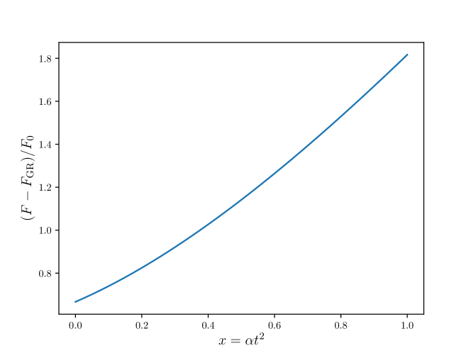
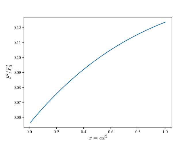
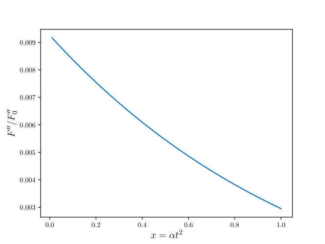
Figure 1: The functions $F$ (upper graph), $F^{\prime}$ (middle graph) and $F^{\prime\prime}$ (lower graph), in terms of the time variable $x$ defined as $x\equiv\alpha t^{2}$, with $F_{\mathrm{GR}}=R$ and $F_{0}=(12\alpha-C)$,$F^{\prime}_{0}=(12\alpha-C)/alpha$ and $F^{\prime\prime}_{0}=(12\alpha-C)/\alpha^{2}$.

III The curvature power spectrum

Since we have studied in the previous section the background behavior of a bouncing scenario realized within $F(R)$ gravity and we have extracted the function $F(R)$ around the bounce, we proceed to the calculation of the curvature power spectrum by deriving the corresponding comoving curvature perturbation.

III.1 The curvature perturbation

Before launching our calculation, we should examine which primordial perturbation modes are relevant for present-day observation. As we saw above, the Hubble parameter vanishes at the bounce point, thus giving rise to an infinite comoving Hubble radius ($1/aH$) there. In the following, we match the bouncing phase with the standard Hot Big Bang radiation phase, which in turn, according to the standard cosmological evolution as dictated by the current cosmological probes, is connected to a matter epoch and then at late times with an accelerated expansion phase. Consequently, the Hubble horizon decreases and tends to zero for late times, while for cosmic times near the bouncing point the Hubble horizon has an infinite size. Therefore, all the perturbation modes at that time are contained within the horizon, and at later epochs they cross the Hubble radius becoming relevant for current observations. Hence, in the following we focus on the perturbation equations near the bounce, namely near $t=0$.

Choosing to work in the comoving gauge, the spatial part of the perturbed scalar metric tensor reads as

$$\delta g_{ij}=a^{2}(t)\big{[}1-2\zeta(\vec{x},t)]\delta_{ij},$$ (13)

where $\zeta(\vec{x},t)$ denotes the comoving curvature perturbation. The corresponding action for the scalar perturbations reads as Hwang:2005hb ; Noh:2001ia ; Hwang:2002fp

$$\delta S_{\zeta}=\int\mathrm{d}t\mathrm{d}^{3}\vec{x}a(t)z(t)^{2}\left[\dot{\zeta}^{2}-\frac{1}{a^{2}}\left(\partial_{i}\zeta\right)^{2}\right]\,,$$ (14)

with $z(t)$ given by the following expression Odintsov:2020zct :

$$z(t)=\frac{a(t)}{\kappa\bigg{[}H(t)+\frac{1}{2F^{\prime}(R)}\frac{dF^{\prime}(R)}{dt}\bigg{]}}\mathchoice{{\hbox{$\displaystyle\sqrt{\frac{3}{2F^{\prime}(R)}\bigg{[}\frac{dF^{\prime}(R)}{dt}\bigg{]}^{2}\,}$}\lower 0.4pt\hbox{\vrule height=17.55444pt,depth=-14.04361pt}}}{{\hbox{$\textstyle\sqrt{\frac{3}{2F^{\prime}(R)}\bigg{[}\frac{dF^{\prime}(R)}{dt}\bigg{]}^{2}\,}$}\lower 0.4pt\hbox{\vrule height=17.55444pt,depth=-14.04361pt}}}{{\hbox{$\scriptstyle\sqrt{\frac{3}{2F^{\prime}(R)}\bigg{[}\frac{dF^{\prime}(R)}{dt}\bigg{]}^{2}\,}$}\lower 0.4pt\hbox{\vrule height=17.03888pt,depth=-13.63116pt}}}{{\hbox{$\scriptscriptstyle\sqrt{\frac{3}{2F^{\prime}(R)}\bigg{[}\frac{dF^{\prime}(R)}{dt}\bigg{]}^{2}\,}$}\lower 0.4pt\hbox{\vrule height=17.03888pt,depth=-13.63116pt}}}.$$ (15)

Using the solution for $F(R)$, i.e. Eq. (8), the expression for $\mathrm{d}F^{\prime}(R)/\mathrm{d}t$ where ^′ denotes differentiation with respect to the Ricci scalar, is given by

$$\frac{\mathrm{d}F^{\prime}(R(t))}{\mathrm{d}t}=\frac{t(12\alpha-C)\left\{t^{2}\alpha(5-t^{2}\alpha)\right\}}{36t^{2}\alpha}$$

$$+\frac{t(12\alpha-C)\left\{\mathchoice{{\hbox{$\displaystyle\sqrt{2\alpha\,}$}\lower 0.4pt\hbox{\vrule height=6.44444pt,depth=-5.15558pt}}}{{\hbox{$\textstyle\sqrt{2\alpha\,}$}\lower 0.4pt\hbox{\vrule height=6.44444pt,depth=-5.15558pt}}}{{\hbox{$\scriptstyle\sqrt{2\alpha\,}$}\lower 0.4pt\hbox{\vrule height=4.51111pt,depth=-3.6089pt}}}{{\hbox{$\scriptscriptstyle\sqrt{2\alpha\,}$}\lower 0.4pt\hbox{\vrule height=3.22221pt,depth=-2.57779pt}}}t[3+t^{2}\alpha(-6+t^{2}\alpha)]F_{\mathrm{D}}\left(\frac{t\mathchoice{{\hbox{$\displaystyle\sqrt{\alpha\,}$}\lower 0.4pt\hbox{\vrule height=3.01389pt,depth=-2.41113pt}}}{{\hbox{$\textstyle\sqrt{\alpha\,}$}\lower 0.4pt\hbox{\vrule height=3.01389pt,depth=-2.41113pt}}}{{\hbox{$\scriptstyle\sqrt{\alpha\,}$}\lower 0.4pt\hbox{\vrule height=2.10971pt,depth=-1.68779pt}}}{{\hbox{$\scriptscriptstyle\sqrt{\alpha\,}$}\lower 0.4pt\hbox{\vrule height=1.50694pt,depth=-1.20557pt}}}}{\mathchoice{{\hbox{$\displaystyle\sqrt{2\,}$}\lower 0.4pt\hbox{\vrule height=4.51111pt,depth=-3.6089pt}}}{{\hbox{$\textstyle\sqrt{2\,}$}\lower 0.4pt\hbox{\vrule height=4.51111pt,depth=-3.6089pt}}}{{\hbox{$\scriptstyle\sqrt{2\,}$}\lower 0.4pt\hbox{\vrule height=3.15778pt,depth=-2.52625pt}}}{{\hbox{$\scriptscriptstyle\sqrt{2\,}$}\lower 0.4pt\hbox{\vrule height=2.25555pt,depth=-1.80446pt}}}}\right)\right\}}{36t^{2}\alpha}.$$

$F^{\prime}(R)$ is given by Eq. (11).

As mentioned earlier, the perturbation modes are generated close to the bounce, therefore we solve the above equation for cosmic times near the bouncing point. As a result, we keep terms upto $\mathcal{O}(\alpha t^{2})$ for the rest of our analysis. The corresponding expression for $z(t)$, keeping terms up to $\mathcal{O}(\alpha t^{2})$ in $F^{\prime}(R)$ and $\frac{\mathrm{d}F^{\prime}(R(t))}{\mathrm{d}t}$, becomes

$$z(t)=\frac{(1/\alpha)^{3/2}\alpha\mathchoice{{\hbox{$\displaystyle\sqrt{12\alpha-C\,}$}\lower 0.4pt\hbox{\vrule height=6.83331pt,depth=-5.46667pt}}}{{\hbox{$\textstyle\sqrt{12\alpha-C\,}$}\lower 0.4pt\hbox{\vrule height=6.83331pt,depth=-5.46667pt}}}{{\hbox{$\scriptstyle\sqrt{12\alpha-C\,}$}\lower 0.4pt\hbox{\vrule height=4.78333pt,depth=-3.82668pt}}}{{\hbox{$\scriptscriptstyle\sqrt{12\alpha-C\,}$}\lower 0.4pt\hbox{\vrule height=3.41666pt,depth=-2.73334pt}}}}{3^{1/2}(t^{2}+1)\kappa}+\frac{2\alpha^{2}\mathchoice{{\hbox{$\displaystyle\sqrt{12\alpha-C\,}$}\lower 0.4pt\hbox{\vrule height=6.83331pt,depth=-5.46667pt}}}{{\hbox{$\textstyle\sqrt{12\alpha-C\,}$}\lower 0.4pt\hbox{\vrule height=6.83331pt,depth=-5.46667pt}}}{{\hbox{$\scriptstyle\sqrt{12\alpha-C\,}$}\lower 0.4pt\hbox{\vrule height=4.78333pt,depth=-3.82668pt}}}{{\hbox{$\scriptscriptstyle\sqrt{12\alpha-C\,}$}\lower 0.4pt\hbox{\vrule height=3.41666pt,depth=-2.73334pt}}}t^{2}}{3^{1/2}4\alpha^{3/2}\kappa}.$$ (17)

At the end, the perturbed action leads to the following Lagrange equation for the Fourier mode of the comoving curvature perturbation, $\zeta_{k}$:

$$\frac{1}{a(t)z^{2}(t)}\frac{d}{dt}\bigg{[}a(t)z^{2}(t)\dot{\zeta}_{k}\bigg{]}+\frac{k^{2}}{a^{2}}\zeta_{k}(t)=0.$$ (18)

In the above equation, by using (17) and keeping terms upto $\mathcal{O}(\alpha t^{2})$, the quantity $a(t)z(t)^{2}$ becomes:

$$a(t)z(t)^{2}=U+Vt^{2},$$ (19)

with $U=\frac{(12\alpha-C)}{12\alpha\kappa^{2}}$, $V=\frac{(12\alpha-C)}{4\kappa^{2}}$.

At the end, the Lagrange equation for $\zeta_{k}$ can be recast at leading order as

$$\ddot{\zeta}_{k}+\frac{2V}{U}t\dot{\zeta}_{k}+k^{2}\zeta_{k}(t)=0,$$ (20)

whose solution is

$$\!\!\!\!\!\!\!\!\!\!\!\!\!\!\!\!\!\zeta_{k}(t)=C_{1}(k)~{}e^{-\frac{V}{U}t^{2}}~{}H\left(-1+\frac{k^{2}U}{2V},\mathchoice{{\hbox{$\displaystyle\sqrt{\frac{V}{U}\,}$}\lower 0.4pt\hbox{\vrule height=10.24997pt,depth=-8.20001pt}}}{{\hbox{$\textstyle\sqrt{\frac{V}{U}\,}$}\lower 0.4pt\hbox{\vrule height=7.17499pt,depth=-5.74002pt}}}{{\hbox{$\scriptstyle\sqrt{\frac{V}{U}\,}$}\lower 0.4pt\hbox{\vrule height=5.12498pt,depth=-4.1pt}}}{{\hbox{$\scriptscriptstyle\sqrt{\frac{V}{U}\,}$}\lower 0.4pt\hbox{\vrule height=5.12498pt,depth=-4.1pt}}}~{}t\right)$$ (21)

$$\ \ +C_{2}(k)~{}e^{-\frac{V}{U}t^{2}}~{}{}_{1}F_{1}\left(\frac{1}{2}-\frac{k^{2}U}{4V},\frac{1}{2},\mathchoice{{\hbox{$\displaystyle\sqrt{\frac{V}{U}\,}$}\lower 0.4pt\hbox{\vrule height=10.24997pt,depth=-8.20001pt}}}{{\hbox{$\textstyle\sqrt{\frac{V}{U}\,}$}\lower 0.4pt\hbox{\vrule height=7.17499pt,depth=-5.74002pt}}}{{\hbox{$\scriptstyle\sqrt{\frac{V}{U}\,}$}\lower 0.4pt\hbox{\vrule height=5.12498pt,depth=-4.1pt}}}{{\hbox{$\scriptscriptstyle\sqrt{\frac{V}{U}\,}$}\lower 0.4pt\hbox{\vrule height=5.12498pt,depth=-4.1pt}}}~{}t^{2}\right),$$

where $C_{1}(k),\ C_{2}(k)$ are integration constants, $H(n,x)$ is the n-th order Hermite polynomial, and ${}_{1}F_{1}(a,b,x)$ is the Kummer confluent hypergeometric function.

The expressions for the integration constants $C_{1}(k),\ C_{2}(k)$ are obtained by setting the initial conditions for the curvature perturbations. Given the fact that close to the bounce the Hubble radius is infinitely large as mentioned above, the primordial modes are well inside the Hubble radius thus satisfying the condition $k\gg aH$. Therefore, the initial conditions for $\zeta_{k}$ will be set through the Mukhanov-Sasaki variable, defined in the present context as $v_{k}(t)\equiv z(t)\zeta_{k}(t)$ Odintsov:2020zct , and whose value on sub-Hubble scales is set by the Bunch-Davies vacuum state, i.e.

$$v_{k,k\ll aH}=\frac{e^{-ik\eta}}{\mathchoice{{\hbox{$\displaystyle\sqrt{2k\,}$}\lower 0.4pt\hbox{\vrule height=6.94444pt,depth=-5.55559pt}}}{{\hbox{$\textstyle\sqrt{2k\,}$}\lower 0.4pt\hbox{\vrule height=6.94444pt,depth=-5.55559pt}}}{{\hbox{$\scriptstyle\sqrt{2k\,}$}\lower 0.4pt\hbox{\vrule height=4.8611pt,depth=-3.8889pt}}}{{\hbox{$\scriptscriptstyle\sqrt{2k\,}$}\lower 0.4pt\hbox{\vrule height=3.47221pt,depth=-2.77779pt}}}},$$ (22)

where the time variable $\eta$ is the conformal time defined by $\mathrm{d}\eta\equiv\mathrm{d}t/a(t)$. Using the expression (5) for the scale factor near the bounce, we obtain from Eq. (22) that

$$\eta=\int^{t}_{0}\mathrm{d}t^{\prime}/a(t^{\prime})=\frac{\arctan(\mathchoice{{\hbox{$\displaystyle\sqrt{\alpha\,}$}\lower 0.4pt\hbox{\vrule height=4.30554pt,depth=-3.44446pt}}}{{\hbox{$\textstyle\sqrt{\alpha\,}$}\lower 0.4pt\hbox{\vrule height=4.30554pt,depth=-3.44446pt}}}{{\hbox{$\scriptstyle\sqrt{\alpha\,}$}\lower 0.4pt\hbox{\vrule height=3.01389pt,depth=-2.41113pt}}}{{\hbox{$\scriptscriptstyle\sqrt{\alpha\,}$}\lower 0.4pt\hbox{\vrule height=2.15277pt,depth=-1.72223pt}}}t)}{\mathchoice{{\hbox{$\displaystyle\sqrt{\alpha\,}$}\lower 0.4pt\hbox{\vrule height=4.30554pt,depth=-3.44446pt}}}{{\hbox{$\textstyle\sqrt{\alpha\,}$}\lower 0.4pt\hbox{\vrule height=4.30554pt,depth=-3.44446pt}}}{{\hbox{$\scriptstyle\sqrt{\alpha\,}$}\lower 0.4pt\hbox{\vrule height=3.01389pt,depth=-2.41113pt}}}{{\hbox{$\scriptscriptstyle\sqrt{\alpha\,}$}\lower 0.4pt\hbox{\vrule height=2.15277pt,depth=-1.72223pt}}}}.$$ (23)

Consequently, the initial conditions satisfied by $v_{k}$ and its derivative become:

$$v_{k}(t\rightarrow 0)=\frac{1}{\mathchoice{{\hbox{$\displaystyle\sqrt{2k\,}$}\lower 0.4pt\hbox{\vrule height=6.94444pt,depth=-5.55559pt}}}{{\hbox{$\textstyle\sqrt{2k\,}$}\lower 0.4pt\hbox{\vrule height=6.94444pt,depth=-5.55559pt}}}{{\hbox{$\scriptstyle\sqrt{2k\,}$}\lower 0.4pt\hbox{\vrule height=4.8611pt,depth=-3.8889pt}}}{{\hbox{$\scriptscriptstyle\sqrt{2k\,}$}\lower 0.4pt\hbox{\vrule height=3.47221pt,depth=-2.77779pt}}}},$$

$$\dot{v}_{k}(t\rightarrow 0)=-\frac{ik\mathchoice{{\hbox{$\displaystyle\sqrt{\alpha\,}$}\lower 0.4pt\hbox{\vrule height=4.30554pt,depth=-3.44446pt}}}{{\hbox{$\textstyle\sqrt{\alpha\,}$}\lower 0.4pt\hbox{\vrule height=4.30554pt,depth=-3.44446pt}}}{{\hbox{$\scriptstyle\sqrt{\alpha\,}$}\lower 0.4pt\hbox{\vrule height=3.01389pt,depth=-2.41113pt}}}{{\hbox{$\scriptscriptstyle\sqrt{\alpha\,}$}\lower 0.4pt\hbox{\vrule height=2.15277pt,depth=-1.72223pt}}}}{\mathchoice{{\hbox{$\displaystyle\sqrt{2k\,}$}\lower 0.4pt\hbox{\vrule height=6.94444pt,depth=-5.55559pt}}}{{\hbox{$\textstyle\sqrt{2k\,}$}\lower 0.4pt\hbox{\vrule height=6.94444pt,depth=-5.55559pt}}}{{\hbox{$\scriptstyle\sqrt{2k\,}$}\lower 0.4pt\hbox{\vrule height=4.8611pt,depth=-3.8889pt}}}{{\hbox{$\scriptscriptstyle\sqrt{2k\,}$}\lower 0.4pt\hbox{\vrule height=3.47221pt,depth=-2.77779pt}}}}.$$ (24)

Using these conditions and the fact that $\dot{z}(t\rightarrow 0)=0$, we finally acquire straightforwardly the expressions for the integration constants $C_{1},\ C_{2}$ as

$$C_{1}(k)=\frac{3i\kappa 2^{\frac{5}{2}-\frac{k^{2}}{6\alpha}}\mathchoice{{\hbox{$\displaystyle\sqrt{k\,}$}\lower 0.4pt\hbox{\vrule height=6.94444pt,depth=-5.55559pt}}}{{\hbox{$\textstyle\sqrt{k\,}$}\lower 0.4pt\hbox{\vrule height=6.94444pt,depth=-5.55559pt}}}{{\hbox{$\scriptstyle\sqrt{k\,}$}\lower 0.4pt\hbox{\vrule height=4.8611pt,depth=-3.8889pt}}}{{\hbox{$\scriptscriptstyle\sqrt{k\,}$}\lower 0.4pt\hbox{\vrule height=3.47221pt,depth=-2.77779pt}}}\alpha^{3/2}\Gamma\left(\frac{3}{2}-\frac{k^{2}}{12\alpha}\right)}{\mathchoice{{\hbox{$\displaystyle\sqrt{\pi\,}$}\lower 0.4pt\hbox{\vrule height=4.30554pt,depth=-3.44446pt}}}{{\hbox{$\textstyle\sqrt{\pi\,}$}\lower 0.4pt\hbox{\vrule height=4.30554pt,depth=-3.44446pt}}}{{\hbox{$\scriptstyle\sqrt{\pi\,}$}\lower 0.4pt\hbox{\vrule height=3.01389pt,depth=-2.41113pt}}}{{\hbox{$\scriptscriptstyle\sqrt{\pi\,}$}\lower 0.4pt\hbox{\vrule height=2.15277pt,depth=-1.72223pt}}}(6\alpha-k^{2})\mathchoice{{\hbox{$\displaystyle\sqrt{12\alpha-C\,}$}\lower 0.4pt\hbox{\vrule height=6.83331pt,depth=-5.46667pt}}}{{\hbox{$\textstyle\sqrt{12\alpha-C\,}$}\lower 0.4pt\hbox{\vrule height=6.83331pt,depth=-5.46667pt}}}{{\hbox{$\scriptstyle\sqrt{12\alpha-C\,}$}\lower 0.4pt\hbox{\vrule height=4.78333pt,depth=-3.82668pt}}}{{\hbox{$\scriptscriptstyle\sqrt{12\alpha-C\,}$}\lower 0.4pt\hbox{\vrule height=3.41666pt,depth=-2.73334pt}}}}$$ (25)

$$\begin{split}C_{2}(k)&=\frac{\mathchoice{{\hbox{$\displaystyle\sqrt{2\,}$}\lower 0.4pt\hbox{\vrule height=6.44444pt,depth=-5.15558pt}}}{{\hbox{$\textstyle\sqrt{2\,}$}\lower 0.4pt\hbox{\vrule height=6.44444pt,depth=-5.15558pt}}}{{\hbox{$\scriptstyle\sqrt{2\,}$}\lower 0.4pt\hbox{\vrule height=4.51111pt,depth=-3.6089pt}}}{{\hbox{$\scriptscriptstyle\sqrt{2\,}$}\lower 0.4pt\hbox{\vrule height=3.22221pt,depth=-2.57779pt}}}\kappa}{k^{1/2}(6\alpha-k^{2})\mathchoice{{\hbox{$\displaystyle\sqrt{12\alpha-C\,}$}\lower 0.4pt\hbox{\vrule height=6.83331pt,depth=-5.46667pt}}}{{\hbox{$\textstyle\sqrt{12\alpha-C\,}$}\lower 0.4pt\hbox{\vrule height=6.83331pt,depth=-5.46667pt}}}{{\hbox{$\scriptstyle\sqrt{12\alpha-C\,}$}\lower 0.4pt\hbox{\vrule height=4.78333pt,depth=-3.82668pt}}}{{\hbox{$\scriptscriptstyle\sqrt{12\alpha-C\,}$}\lower 0.4pt\hbox{\vrule height=3.41666pt,depth=-2.73334pt}}}\Gamma\left(1-\frac{k^{2}}{12\alpha}\right)}\Bigl{[}-6ik\alpha^{3/2}\\ &\times\Gamma\left(\frac{3}{2}-\frac{k^{2}}{12\alpha}\right)+\mathchoice{{\hbox{$\displaystyle\sqrt{3\alpha\,}$}\lower 0.4pt\hbox{\vrule height=6.44444pt,depth=-5.15558pt}}}{{\hbox{$\textstyle\sqrt{3\alpha\,}$}\lower 0.4pt\hbox{\vrule height=6.44444pt,depth=-5.15558pt}}}{{\hbox{$\scriptstyle\sqrt{3\alpha\,}$}\lower 0.4pt\hbox{\vrule height=4.51111pt,depth=-3.6089pt}}}{{\hbox{$\scriptscriptstyle\sqrt{3\alpha\,}$}\lower 0.4pt\hbox{\vrule height=3.22221pt,depth=-2.57779pt}}}\left(6\alpha-k^{2}\right)\Gamma\left(1-\frac{k^{2}}{12\alpha}\right)\Bigr{]},\end{split}$$ (26)

where $\Gamma(x)$ denotes the Gamma function. At the end, the corresponding curvature power spectrum can be recast as follows:

$$\!\!\!\!\!\!\!\!\!\!\!\!\!\!\!\!\!\!\!\!\!\!\!\!\!\!\!\!\!\begin{split}\mathcal{P}_{\zeta}(k,t)&\equiv\frac{k^{3}}{2\pi^{2}}~{}\bigg{|}\zeta_{k}(t)\bigg{|}^{2}\\ &=\frac{k^{3}}{2\pi^{2}}~{}\bigg{|}C_{1}(k)~{}e^{-\frac{V}{U}t^{2}}~{}H\bigg{[}-1+\frac{k^{2}U}{2V},\mathchoice{{\hbox{$\displaystyle\sqrt{\frac{V}{U}\,}$}\lower 0.4pt\hbox{\vrule height=10.24997pt,depth=-8.20001pt}}}{{\hbox{$\textstyle\sqrt{\frac{V}{U}\,}$}\lower 0.4pt\hbox{\vrule height=7.17499pt,depth=-5.74002pt}}}{{\hbox{$\scriptstyle\sqrt{\frac{V}{U}\,}$}\lower 0.4pt\hbox{\vrule height=5.12498pt,depth=-4.1pt}}}{{\hbox{$\scriptscriptstyle\sqrt{\frac{V}{U}\,}$}\lower 0.4pt\hbox{\vrule height=5.12498pt,depth=-4.1pt}}}~{}t\bigg{]}\\ &+C_{2}(k)~{}e^{-\frac{V}{U}t^{2}}~{}{}_{1}F_{1}\bigg{[}\frac{1}{2}-\frac{k^{2}U}{4V},\frac{1}{2},\mathchoice{{\hbox{$\displaystyle\sqrt{\frac{V}{U}\,}$}\lower 0.4pt\hbox{\vrule height=10.24997pt,depth=-8.20001pt}}}{{\hbox{$\textstyle\sqrt{\frac{V}{U}\,}$}\lower 0.4pt\hbox{\vrule height=7.17499pt,depth=-5.74002pt}}}{{\hbox{$\scriptstyle\sqrt{\frac{V}{U}\,}$}\lower 0.4pt\hbox{\vrule height=5.12498pt,depth=-4.1pt}}}{{\hbox{$\scriptscriptstyle\sqrt{\frac{V}{U}\,}$}\lower 0.4pt\hbox{\vrule height=5.12498pt,depth=-4.1pt}}}~{}t^{2}\bigg{]}\bigg{|}^{2}.\end{split}$$ (27)

III.2 Matching the bounce with a radiation-dominated era

As explained in Sec. II, close to the bounce the underlying gravity theory is described by a $F(R)$ modified gravity setup with $F(R)$ given by Eq. (8). During this phase, the scale factor evolution is dictated by Eq. (5), which is nothing else than a perturbative expansion close to the bounce, valid for $\alpha t^{2}\lesssim 1$, and corresponds to a fluid dominated Universe with an equation-of-state parameter $w=-2/3$. Then, $F(R)$ gravity modifications are switched off and one recovers the standard HBB phase which is described by GR. Consequently, matching the two phases and requiring continuity of the scale factor at the onset of the RD era one gets that

$$a(t)=\begin{cases}1+\alpha t^{2}\mathrm{\;,\;}t<t_{\mathrm{RD}}\\ a_{\mathrm{RD}}\left(\frac{t}{t_{\mathrm{RD}}}\right)^{1/2}\mathrm{\;,\;}t>t_{\mathrm{RD}},\end{cases}$$ (28)

with $t_{\mathrm{RD}}$ being the transition time between the exotic phase close to the bounce with $w=-2/3$ and the RD phase given by Eq. (9), and $a_{\mathrm{RD}}$ the respective scale factor at the onset of the RD era. We mention that in order to keep the scale factor continuous during the transition we choose $a_{\mathrm{RD}}$ to be $a_{\mathrm{RD}}=1+\alpha t^{2}_{\mathrm{RD}}$.

Given the fact that in the following we elaborate the power spectrum at the horizon crossing time during the RD era, i.e. $k=a(t)H(t)$ with $t>t_{\mathrm{RD}}$, one can find the horizon crossing time $t_{\mathrm{HC}}(k,\alpha)$ by solving $k=aH$ with $a(t)=a_{\mathrm{RD}}\left(\frac{t}{t_{\mathrm{RD}}}\right)^{1/2}$ and $H(t)=\frac{1}{2t}$. At the end, we extract that

$$t_{\mathrm{HC}}(k,\alpha)=\frac{\mathchoice{{\hbox{$\displaystyle\sqrt{\alpha\,}$}\lower 0.4pt\hbox{\vrule height=4.30554pt,depth=-3.44446pt}}}{{\hbox{$\textstyle\sqrt{\alpha\,}$}\lower 0.4pt\hbox{\vrule height=4.30554pt,depth=-3.44446pt}}}{{\hbox{$\scriptstyle\sqrt{\alpha\,}$}\lower 0.4pt\hbox{\vrule height=3.01389pt,depth=-2.41113pt}}}{{\hbox{$\scriptscriptstyle\sqrt{\alpha\,}$}\lower 0.4pt\hbox{\vrule height=2.15277pt,depth=-1.72223pt}}}}{k^{2}}.$$ (29)

At this point it is important to stress out that in the expression (27) we derived the curvature power spectrum close to the bounce by parametrizing the scale factor as in Eq. (5). Eq. (5) describes actually quite well the background dynamical evolution up to the onset of the RD era when the perturbative expansion of the scale factor breaks down. Hence, one can compute $\mathcal{P}_{\zeta}(k,t)$ at horizon exiting time during the initial $F(R)$ gravity phase before the RD era, namely when $k=a(t)H(t)$ with $t<t_{\mathrm{RD}}$. At this point, we need to stress that in general within the context of bouncing cosmologies, as we pass from the contraction to the expansion phase the comoving curvature perturbation $\zeta_{k}$ is not necessarily conserved Battefeld:2014uga . However, for non-singular bouncing scenarios as the one we consider here one finds a non-singular evolution of $\zeta_{k}$ through the bounce Allen:2004vz ; Cartier:2003jz and a conservation of the curvature perturbation on superhorizon scales during the expanding phase Peter:2002cn ; Kumar:2013koa ; Battarra:2014tga . The conservation of $\zeta_{k}$ on superhorizon scales can be viewed as well as a consequence of the local energy conservation which is valid for any relativistic gravitational theory Lyth:2004gb ; Wands:2000dp . In view of these considerations, the curvature power spectrum at horizon crossing time during the RD era will be the same as the curvature power spectrum at horizon exiting time during the initial $F(R)$ gravity phase between the bounce and the RD era, namely

$$\mathcal{P}_{\zeta}\left[k,t_{\mathrm{HC}}(k,\alpha)\right]=\mathcal{P}_{\zeta}\left[k,t_{\mathrm{exit}}(k,\alpha)\right],$$ (30)

where $t_{\mathrm{HC}}(k,\alpha)$ is given by (29) and $t_{\mathrm{exit}}(k,\alpha)=\frac{k}{2\alpha}$. Finally, we can then use $\mathcal{P}_{\zeta}\left[k,t_{\mathrm{HC}}(k,\alpha)\right]$ and proceed to the calculation of the PBH abundance at horizon crossing time during the RD era, which is considered to be the PBH formation time.

III.3 The scales involved

Regarding the relevant scales for the problem at hand, here we consider modes whose first horizon crossing time, i.e. when the modes exit the horizon, occurs before the RD era, that is $t_{\mathrm{exit}}<t_{\mathrm{RD}}$. Thus, accounting for the fact that $t_{\mathrm{exit}}(k,\alpha)=\frac{k}{2\alpha}$ and $t_{\mathrm{RD}}=1/\mathchoice{{\hbox{$\displaystyle\sqrt{\alpha\,}$}\lower 0.4pt\hbox{\vrule height=4.30554pt,depth=-3.44446pt}}}{{\hbox{$\textstyle\sqrt{\alpha\,}$}\lower 0.4pt\hbox{\vrule height=4.30554pt,depth=-3.44446pt}}}{{\hbox{$\scriptstyle\sqrt{\alpha\,}$}\lower 0.4pt\hbox{\vrule height=3.01389pt,depth=-2.41113pt}}}{{\hbox{$\scriptscriptstyle\sqrt{\alpha\,}$}\lower 0.4pt\hbox{\vrule height=2.15277pt,depth=-1.72223pt}}}$, one can trivially find an upper bound on the comoving scale $k$ reading as

$$k<2\mathchoice{{\hbox{$\displaystyle\sqrt{\alpha\,}$}\lower 0.4pt\hbox{\vrule height=4.30554pt,depth=-3.44446pt}}}{{\hbox{$\textstyle\sqrt{\alpha\,}$}\lower 0.4pt\hbox{\vrule height=4.30554pt,depth=-3.44446pt}}}{{\hbox{$\scriptstyle\sqrt{\alpha\,}$}\lower 0.4pt\hbox{\vrule height=3.01389pt,depth=-2.41113pt}}}{{\hbox{$\scriptscriptstyle\sqrt{\alpha\,}$}\lower 0.4pt\hbox{\vrule height=2.15277pt,depth=-1.72223pt}}}.$$ (31)

This upper bound on $k$ is equivalent with a minimum PBH mass. In particular, considering the fact that the PBH mass is roughly the mass within the cosmological horizon at horizon crossing time during the RD era, one can trivially find that

$$M>\frac{2\pi M_{\scriptscriptstyle{\mathrm{Pl}}}^{2}}{\mathchoice{{\hbox{$\displaystyle\sqrt{\alpha\,}$}\lower 0.4pt\hbox{\vrule height=4.30554pt,depth=-3.44446pt}}}{{\hbox{$\textstyle\sqrt{\alpha\,}$}\lower 0.4pt\hbox{\vrule height=4.30554pt,depth=-3.44446pt}}}{{\hbox{$\scriptstyle\sqrt{\alpha\,}$}\lower 0.4pt\hbox{\vrule height=3.01389pt,depth=-2.41113pt}}}{{\hbox{$\scriptscriptstyle\sqrt{\alpha\,}$}\lower 0.4pt\hbox{\vrule height=2.15277pt,depth=-1.72223pt}}}}$$ (32)

IV The PBH Formation Formalism

In this section we present a general formalism for the computation of the mass function of PBHs formed due to the collapse of enhanced cosmological perturbations once they reenter the cosmological horizon. Basically, this happens when the energy density contrast of the collapsing overdensity region, or the respective comoving curvature perturbation, becomes greater than a critical threshold $\delta_{\mathrm{c}}$ or $\zeta_{\mathrm{c}}$. In the following, we firstly describe how the comoving curvature perturbation is connected to the energy density contrast, extracting the non-linear relation between them, and then we proceed by presenting the formalism for the computation of the PBH mass function and the PBH abundance within the context of peak theory Bardeen:1985tr . At this point, it is important to highlight that we study PBH formation during the standard RD era described by general relativity. Therefore, the use of the peak theory formalism, developed within GR, for the computation of the PBH abundance is absolutely legitimate within our work.

IV.1 From the comoving curvature perturbation to the energy density contrast

Assuming spherical symmetry on superhorizon scales , the local region of the universe describing the aforementioned collapsing cosmological perturbations is described by the following asymptotic form of the metric

$$\mathrm{d}s^{2}=-\mathrm{d}t^{2}+a^{2}(t)e^{\zeta(r)}\left[\mathrm{d}r^{2}+r^{2}\mathrm{d}\Omega^{2}\right],$$ (33)

where $a(t)$ is the scale factor and $\zeta(r)$ is the comoving curvature perturbation which is conserved on superhorizon scales. In this regime one can perform a gradient expansion approximation, where all the hydrodynamic and metric quantities are nearly homogeneous, and their perturbations are small deviations away from their background values Shibata_1999 ; Salopek:1990jq ; Wands:2000dp ; Lyth:2004gb . In this approximation, the energy density perturbation profile is related to the comoving curvature perturbation through the following expression Harada:2015yda ; Yoo:2018kvb ; Musco:2018rwt :

$$\frac{\delta\rho}{\rho_{\mathrm{b}}} \equiv\frac{\rho(r,t)-\rho_{\mathrm{b}}(t)}{\rho_{\mathrm{b}}(t)}$$

$$=-\left(\frac{1}{aH}\right)^{2}\frac{4(1+w)}{5+3w}e^{-5\zeta(r)/2}\nabla^{2}e^{\zeta(r)/2},$$ (34)

where $w$ is the total equation-of-state parameter defined as the ratio between the total pressure $p$ and the total energy density $\rho$, i.e. $w\equiv p/\rho$. In the linear regime, where $\zeta\ll 1$, the above expression is reduced to

$$\frac{\delta\rho}{\rho_{\mathrm{b}}} \simeq-\frac{1}{a^{2}H^{2}}\frac{2(1+w)}{5+3w}\nabla^{2}\zeta(r)$$

$$\Longrightarrow\delta_{k}=-\frac{k^{2}}{a^{2}H^{2}}\frac{2(1+w)}{5+3w}\zeta_{k}.$$ (35)

Note that the last expression is obtained by Fourier transforming the energy density contrast $\delta$ and the curvature perturbation $\zeta$.

From the above form we can see that there is a one-to-one relation between the comoving curvature perturbation and the energy density contrast. Thus, if the curvature perturbation is a Gaussian variable then the same is true for the density contrast within the linear regime described by (IV.1). However, the amplitude of the critical threshold $\delta_{\mathrm{c}}$ or $\zeta_{\mathrm{c}}$ is in general non-linear, and as a consequence one should consider the full non-linear expression between $\zeta$ and $\delta$, namely (IV.1).

Here it is very important to stress that within the context of bouncing cosmological scenarios one expects in general the presence of non Gaussianities with an amplitude larger than the one predicted in simple inflationary setups Quintin:2015rta ; Gao:2014eaa . In particular, for our case for perturbations whose first horizon crossing is before the onset of the RD era, the curvature perturbation $\zeta$ will become super-horizon during the intermediate exotic contracting phase with $w=-2/3$ possibly developing non-Gaussianity and eventually becoming highly non linear. After the onset of the RD era, due to the conservation of $\zeta$ in the expanding phase, it will remain constant. In view of these considerations we assume that the curvature perturbation field remains Gaussian and linear (to avoid breaking of perturbation theory) during the intermediate phase which connects the bounce with the RD era Cai:2009fn .

At this point, we should also highlight the fact that the use of $\zeta$ for the computation of the PBH abundance vastly overestimates the number of PBHs, since scales larger than the PBH scale, which are unobservable, are not properly removed when the PBH distribution is smoothed Young:2014ana . Therefore, one should instead use the energy density contrast, given the fact that with this prescription the superhorizon scales are naturally damped by $k^{2}$, as it can be seen by (IV.1).

From a mathematical point of view, by performing a coordinate transformation on superhorizon scales, one can always shift the comoving curvature perturbation by an arbitrary constant, making the calculation of the PBH abundance not physical. On the other hand, if the density contrast is adopted instead, a dependence on spatial derivatives of the curvature perturbation is obtained as it can be seen by Eq. (IV.1), making the problem physical. This is another way to see that the choice to work with $\delta$ instead of $\zeta$ for the computation of the PBH abundance is the correct one.

Consequently, smoothing the energy density contrast with a Gaussian window function over scales smaller than the horizon scale and using (IV.1), we can straightforwardly find that the smoothed energy density contrast is related to the comoving curvature perturbation in radiation era, where $w=1/3$, as Young:2019yug

$$\delta_{\mathrm{m}}=-\frac{2}{3}r_{\mathrm{m}}\zeta^{\prime}(r_{\mathrm{m}})\left[2+r_{\mathrm{m}}\zeta^{\prime}(r_{\mathrm{m}})\right].$$ (36)

The scale $r_{\mathrm{m}}$ is the comoving scale of the collapsing overdensity, which can be found by maximizing the compaction function $\mathcal{C}$ defined as Musco:2018rwt

$$\mathcal{C}(r,t)\equiv 2\frac{M(r,t)-M_{\mathrm{b}}(r,t)}{R(r,t)},$$ (37)

where $R(r,t)$ is the areal radius, $M(r,t)$ is the Misner-Sharp mass Misner:1964je ; Hayward:1994bu within a sphere of a radius $R$, and $M_{\mathrm{b}}=4\pi R^{3}(r,t)/3$ is the background mass with respect to a FLRW metric. Finally, by maximizing the compaction function, namely $\mathcal{C}^{\prime}(r_{\mathrm{m}})=0$, the $r_{\mathrm{m}}$ scale will be given by the solution of the following equation:

$$\zeta^{\prime}(r_{\mathrm{m}})+r_{\mathrm{m}}\zeta(r_{\mathrm{m}})=0.$$ (38)

Now, given the fact that $\zeta$ is assumed to have a Gaussian distribution, its derivative will have a Gaussian distribution too. Hence, we can identify a linear Gaussian variable $\delta_{l}=-\frac{4}{3}r_{\mathrm{m}}\zeta^{\prime}(r_{\mathrm{m}})$ with a probability distribution function (PDF) given by

$$P(\delta_{l})=\frac{1}{\mathchoice{{\hbox{$\displaystyle\sqrt{2\pi\sigma\,}$}\lower 0.4pt\hbox{\vrule height=6.44444pt,depth=-5.15558pt}}}{{\hbox{$\textstyle\sqrt{2\pi\sigma\,}$}\lower 0.4pt\hbox{\vrule height=6.44444pt,depth=-5.15558pt}}}{{\hbox{$\scriptstyle\sqrt{2\pi\sigma\,}$}\lower 0.4pt\hbox{\vrule height=4.51111pt,depth=-3.6089pt}}}{{\hbox{$\scriptscriptstyle\sqrt{2\pi\sigma\,}$}\lower 0.4pt\hbox{\vrule height=3.22221pt,depth=-2.57779pt}}}}e^{-\frac{\delta^{2}_{l}}{2\sigma^{2}}},$$ (39)

where $\sigma$ is the smoothed variance of $\delta_{l}$ written as

$$\sigma^{2} \equiv\langle\delta^{2}_{l}\rangle=\int_{0}^{\infty}\frac{\mathrm{d}k}{k}\mathcal{P}_{\delta_{l}}(k,R)$$

$$=\frac{16}{81}\int_{0}^{\infty}\frac{\mathrm{d}k}{k}(kR)^{4}\tilde{W}^{2}(k,R)\mathcal{P}_{\zeta}(k).$$ (40)

The function $\tilde{W}(k,R)$ is the Fourier transformation of a Gaussian window function  and reads as

$$\tilde{W}(k,R)=e^{-k^{2}R^{2}/2},$$ (41)

Finally, the smoothed energy density contrast is related with the linear Gaussian energy density contrast through the following expression DeLuca:2019qsy ; Young:2019yug :

$$\delta_{\mathrm{m}}=\delta_{l}-\frac{3}{8}\delta^{2}_{l}.$$ (42)

IV.2 The PBH mass function within peak theory

In order to extract the mass function of PBHs which form due to the gravitational collapse of non-Gaussian energy density perturbations, we work with the Gaussian component of the smoothed non-Gaussian energy density contrast denoted as $\delta_{l}$. Regarding the critical threshold of the linear Gaussian component, this can be found by solving Eq. (42) for $\delta_{l}$ with $\delta_{\mathrm{m}}=\delta_{\mathrm{c}}$. Hence, we find that

$$\delta_{\mathrm{c},l\pm}=\frac{4}{3}\left(1\pm\mathchoice{{\hbox{$\displaystyle\sqrt{\frac{2-3\delta_{\mathrm{c}}}{2}\,}$}\lower 0.4pt\hbox{\vrule height=11.37221pt,depth=-9.09781pt}}}{{\hbox{$\textstyle\sqrt{\frac{2-3\delta_{\mathrm{c}}}{2}\,}$}\lower 0.4pt\hbox{\vrule height=7.97777pt,depth=-6.38225pt}}}{{\hbox{$\scriptstyle\sqrt{\frac{2-3\delta_{\mathrm{c}}}{2}\,}$}\lower 0.4pt\hbox{\vrule height=5.94443pt,depth=-4.75557pt}}}{{\hbox{$\scriptscriptstyle\sqrt{\frac{2-3\delta_{\mathrm{c}}}{2}\,}$}\lower 0.4pt\hbox{\vrule height=5.94443pt,depth=-4.75557pt}}}\right).$$ (43)

From the above expression we acquire a critical threshold for $\delta_{l}$. As explained in Young:2019yug , only $\delta_{\mathrm{c},l-}$ corresponds to a physical solution, and since the argument of the square root should be positive we require $\delta_{\mathrm{c}}<2/3$. In summary, we find that the physical range of $\delta_{l}$ is $\delta_{\mathrm{c},l-}<\delta_{l}<4/3$.

Regarding the PBH mass, it should be of the order of the horizon mass at PBH formation time, which is considered as the horizon crossing time. More precisely, the PBH mass spectrum, as it has been shown in Niemeyer:1997mt ; Niemeyer:1999ak ; Musco:2008hv ; Musco:2012au , should follow a critical collapse scaling law which can be recast as

$$M_{\mathrm{PBH}}=M_{\mathrm{H}}\mathcal{K}(\delta-\delta_{\mathrm{c}})^{\gamma},$$ (44)

where $M_{\mathrm{H}}$ is the mass within the cosmological horizon at horizon crossing time, and $\gamma$ is the critical exponent which depends on the equation-of-state parameter at the time of PBH formation and for radiation it is $\gamma\simeq 0.36$. The parameter $\mathcal{K}$ is a parameter that depends on the equation-of-state parameter and on the particular shape of the collapsing overdensity region. In the following we consider a representative value of $\mathcal{K}\simeq 4$.

Concerning now the value of the PBH formation threshold $\delta_{\mathrm{c}}$, its value should vary roughly within the range $0.4\lesssim\delta_{\mathrm{c}}\lesssim 0.6$ depending on the shape of the curvature power spectrum $\mathcal{P}_{\zeta}(k)$. Following the procedure developed in Musco:2020jjb we found that for the values of $\alpha$ studied here, namely for $\alpha\in[10^{-24}M_{\scriptscriptstyle{\mathrm{Pl}}}^{2}\leq\alpha\leq 10^{-14}M_{\scriptscriptstyle{\mathrm{Pl}}}^{2}]$, $\delta_{\mathrm{c}}\simeq 0.5898$ independently of the value of $\alpha$. This is somehow expected since as it can be seen from Fig. 2 the shape of $\mathcal{P}_{\zeta}(k)$ slightly changes with respect to $\alpha$. In particular, as one varies $\alpha$, we observe a change in terms of the overall amplitude of $\mathcal{P}_{\zeta}(k)$ and not in terms of its shape.

Thus, working with the Gaussian linear component of the energy density contrast, we can calculate the PBH abundance in the context of peak theory, where the density of sufficiently rare and large peaks for a random Gaussian density field in spherical symmetry is given by Bardeen:1985tr

$$\mathcal{N}(\nu)=\frac{\mu^{3}}{4\pi^{2}}\frac{\nu^{3}}{\sigma^{3}}e^{-\nu^{2}/2}.$$ (45)

In this expression, $\nu\equiv\delta/\sigma$ and $\sigma$ is given by (IV.1), while the parameter $\mu$ is the first moment of the smoothed power spectrum given by

$$\mu^{2} =\int_{0}^{\infty}\frac{\mathrm{d}k}{k}\mathcal{P}_{\delta_{l}}(k,R)\left(\frac{k}{aH}\right)^{2}=$$

$$\frac{16}{81}\int_{0}^{\infty}\frac{\mathrm{d}k}{k}(kR)^{4}\tilde{W}^{2}(k,R)\mathcal{P}_{\zeta}(k)\left(\frac{k}{aH}\right)^{2}.$$ (46)

Finally, the fraction $\beta_{\nu}$ of the energy of the universe at a peak of a given height $\nu$, which collapses to form a PBH, will be given by

$$\beta_{\nu}=\frac{M_{\mathrm{PBH}}(\nu)}{M_{\mathrm{H}}}\mathcal{N}(\nu)\Theta(\nu-\nu_{\mathrm{c}})$$ (47)

and the total energy fraction of the universe contained in PBHs of mass $M$ can be recast as

$$\beta(M)=\int_{\nu_{\mathrm{c-}}}^{\frac{4}{3\sigma}}\mathrm{d}\nu\frac{\mathcal{K}}{4\pi^{2}}\left(\nu\sigma-\frac{3}{8}\nu^{2}\sigma^{2}-\delta_{\mathrm{c}}\right)^{\gamma}\left(\frac{\mu}{\sigma}\right)^{3}\nu^{3}e^{-\nu^{2}/2},$$ (48)

where $\nu_{\mathrm{c-}}=\delta_{\mathrm{c},l}/\sigma$. Lastly, the overall PBH abundance, defined as $\Omega_{\mathrm{PBH}}\equiv\frac{\rho_{\mathrm{PBH}}}{\rho_{\mathrm{tot}}}$, where $\rho_{\mathrm{tot}}$ is the total energy density of the universe, will be the integrated PBH mass function. Thus, at time $t$ during the RD era, $\Omega_{\mathrm{PBH}}$ will be recast as

$$\Omega_{\mathrm{PBH}}(t)=\int_{M_{\mathrm{min}}}^{M_{\mathrm{max}}}\left(\frac{M_{\mathrm{H}}(t)}{M}\right)^{1/2}\beta(M)\mathrm{d}\ln M,$$ (49)

where $M_{\mathrm{H}}(t)$ is the mass within the cosmological horizon at time $t$. Note that in Eq. (49) we have accounted for the fact that during the RD era $M_{\mathrm{H}}\sim a^{2}$.

V Results

In the previous sections we extracted the curvature power spectrum and we presented the mathematical setup through which one can calculate the PBH mass function and abundance during the standard RD era which follows the exotic $F(R)$ gravity phase close to the bounce. Thus, in this section we present the main results of our work. Initially, we study the behaviour of the curvature power spectrum by varying the parameters of the problem at hand, namely the bouncing parameter $\alpha$. Then, we compute numerically the PBH mass function and we show how it varies by changing $\alpha$. Finally, by demanding that GWs induced from PBH Poisson fluctuations during an early PBH dominated era before BBN are not overproduced, we set constraints on $\alpha$.

V.1 The curvature power spectrum

Given the fact that the scales collapsing to PBHs are initially super-Hubble before crossing the Hubble radius and collapse to PBHs, we perform a Taylor expansion of the comoving curvature perturbation (21) on super-Hubble scales, i.e. when $k\ll aH$. By keeping terms up to $\mathcal{O}\left[\left(\frac{k}{aH}\right)^{3/2}\right]$ we obtain that

$$\zeta_{k,k\ll aH}\simeq\kappa e^{3\alpha t^{2}}\mathchoice{{\hbox{$\displaystyle\sqrt{\frac{3}{t(12\alpha-C)}\,}$}\lower 0.4pt\hbox{\vrule height=11.44444pt,depth=-9.1556pt}}}{{\hbox{$\textstyle\sqrt{\frac{3}{t(12\alpha-C)}\,}$}\lower 0.4pt\hbox{\vrule height=8.01111pt,depth=-6.40892pt}}}{{\hbox{$\scriptstyle\sqrt{\frac{3}{t(12\alpha-C)}\,}$}\lower 0.4pt\hbox{\vrule height=5.72221pt,depth=-4.57779pt}}}{{\hbox{$\scriptscriptstyle\sqrt{\frac{3}{t(12\alpha-C)}\,}$}\lower 0.4pt\hbox{\vrule height=5.72221pt,depth=-4.57779pt}}}\left[\frac{k}{a(t)H(t)}\right]^{-1/2}$$

$$-i\frac{\kappa\alpha t}{\mathchoice{{\hbox{$\displaystyle\sqrt{t(12\alpha-C)\,}$}\lower 0.4pt\hbox{\vrule height=7.5pt,depth=-6.00003pt}}}{{\hbox{$\textstyle\sqrt{t(12\alpha-C)\,}$}\lower 0.4pt\hbox{\vrule height=7.5pt,depth=-6.00003pt}}}{{\hbox{$\scriptstyle\sqrt{t(12\alpha-C)\,}$}\lower 0.4pt\hbox{\vrule height=5.25pt,depth=-4.20003pt}}}{{\hbox{$\scriptscriptstyle\sqrt{t(12\alpha-C)\,}$}\lower 0.4pt\hbox{\vrule height=3.75pt,depth=-3.00002pt}}}}\left[e^{3\alpha t^{2}}\mathchoice{{\hbox{$\displaystyle\sqrt{\pi\,}$}\lower 0.4pt\hbox{\vrule height=4.30554pt,depth=-3.44446pt}}}{{\hbox{$\textstyle\sqrt{\pi\,}$}\lower 0.4pt\hbox{\vrule height=4.30554pt,depth=-3.44446pt}}}{{\hbox{$\scriptstyle\sqrt{\pi\,}$}\lower 0.4pt\hbox{\vrule height=3.01389pt,depth=-2.41113pt}}}{{\hbox{$\scriptscriptstyle\sqrt{\pi\,}$}\lower 0.4pt\hbox{\vrule height=2.15277pt,depth=-1.72223pt}}}-2H\left(-1,t\mathchoice{{\hbox{$\displaystyle\sqrt{3\alpha\,}$}\lower 0.4pt\hbox{\vrule height=6.44444pt,depth=-5.15558pt}}}{{\hbox{$\textstyle\sqrt{3\alpha\,}$}\lower 0.4pt\hbox{\vrule height=6.44444pt,depth=-5.15558pt}}}{{\hbox{$\scriptstyle\sqrt{3\alpha\,}$}\lower 0.4pt\hbox{\vrule height=4.51111pt,depth=-3.6089pt}}}{{\hbox{$\scriptscriptstyle\sqrt{3\alpha\,}$}\lower 0.4pt\hbox{\vrule height=3.22221pt,depth=-2.57779pt}}}\right)\right]\mathchoice{{\hbox{$\displaystyle\sqrt{\frac{k}{a(t)H(t)}\,}$}\lower 0.4pt\hbox{\vrule height=11.94444pt,depth=-9.5556pt}}}{{\hbox{$\textstyle\sqrt{\frac{k}{a(t)H(t)}\,}$}\lower 0.4pt\hbox{\vrule height=8.3611pt,depth=-6.68892pt}}}{{\hbox{$\scriptstyle\sqrt{\frac{k}{a(t)H(t)}\,}$}\lower 0.4pt\hbox{\vrule height=5.97221pt,depth=-4.7778pt}}}{{\hbox{$\scriptscriptstyle\sqrt{\frac{k}{a(t)H(t)}\,}$}\lower 0.4pt\hbox{\vrule height=5.97221pt,depth=-4.7778pt}}}$$

$$-\frac{\kappa\alpha t^{3/2}}{\mathchoice{{\hbox{$\displaystyle\sqrt{3(12\alpha-C\,}$}\lower 0.4pt\hbox{\vrule height=7.5pt,depth=-6.00003pt}}}{{\hbox{$\textstyle\sqrt{3(12\alpha-C\,}$}\lower 0.4pt\hbox{\vrule height=7.5pt,depth=-6.00003pt}}}{{\hbox{$\scriptstyle\sqrt{3(12\alpha-C\,}$}\lower 0.4pt\hbox{\vrule height=5.25pt,depth=-4.20003pt}}}{{\hbox{$\scriptscriptstyle\sqrt{3(12\alpha-C\,}$}\lower 0.4pt\hbox{\vrule height=3.75pt,depth=-3.00002pt}}}}{}_{1}F^{(1,0,0)}_{1}\left(\frac{1}{2},\frac{1}{2},3\alpha t^{2}\right)\left[\frac{k}{a(t)H(t)}\right]^{3/2},$$ (50)

where ${}_{1}F^{(1,0,0)}_{1}(x,y,z)$ stands for the derivative of the Kummer confluent hypergeometric function with respect to its first argument.

Therefore, inserting this expression in Eq. (27) and following the procedure described in Sec. IV, we can calculate the curvature power spectrum $\mathcal{P}_{\zeta}(k)$ at horizon crossing time by fixing the bouncing parameter $\alpha$ and the integration constant $C$. As it was checked numerically, $\mathcal{P}_{\zeta}(k)$ is independent on the value of $C$ and in the following we will fix its value to $C=0.1\alpha$. In the following, we will use the above expression for $\zeta_{k,k\ll aH}$ when computing the comoving curvature perturbation and subsequently the matter power spectrum $\mathcal{P}_{\delta}(k)$ following the procedure described in Sec. IV. As it was confirmed numerically the curvature power spectrum $\mathcal{P}_{\zeta}(k)$ computed using Eq. (V.1) matches quite well the exact $\mathcal{P}_{\zeta}(k)$ all along the $k$ range.

In Fig. 2, we depict the curvature power spectrum $\mathcal{P}_{\zeta}(k)$ [Eq. (27)] on superhorizon scales, for different values of $\alpha$ and for $C=0.1\alpha$. As we can see, the power spectrum increases by increasing the value of $\alpha$. This behaviour can be understood if one sees how the maximum allowed value of $k$, which corresponds to the lowest scale of the problem at hand, varies with $\alpha$. In particular, as we can see from Eq. (31), the value of $k_{\mathrm{max}}$ increases with an increase of $\alpha$, hence the power spectrum shifts to higher values of $k$, i.e. to smaller scales. Consequently, as approaching smaller and smaller scales one starts to probe the granularity of the energy density field, entering in this way the non linear regime where $\mathcal{P}_{\mathrm{\zeta}}(k)\gg 1$. Hence, one can clearly understand the tendency of the power spectrum to increase with increasing $\alpha$, given the fact that it probes smaller scales which become non-linear.

In order to avoid the presence of non linearities, one could abruptly cut the curvature power spectrum at values smaller than unity in order to ensure the validity of the linear perturbative regime. However, given the fact that PBH formation is a non-linear process since it takes place in overdensity regions where $\delta>\delta_{\mathrm{c}}\sim\mathcal{O}(1)$ the introduction of an abrupt cutoff would dramatically decrease the PBH abundance to values orders of magnitude smaller than its real value. The correct way to remove these non-linear scales is actually through the introduction of the non-linear transfer function which has not yet been extracted and requires high cost $N$ body simulations which go beyond the scope of this work Young:2019osy . Consequently, as it is standardly adopted within the context of the PBH literature, these small non-linear scales are naturally smoothed out when computing the PBH mass function through the use of a window function introduced in Sec. IV.

Figure 2: The curvature power spectrum versus $k$ for different values of $\alpha$.

V.2 The PBH mass function

Since we have extracted above the curvature power spectra for different values of $\alpha$, we proceed to the calculation of the PBH mass function within peak theory. In particular, we follow the mathematical formalism presented in Sec. IV.2, accounting for the non-linear relation between $\delta$ and $\zeta$ as well as the critical collapse law for the PBH masses. Below, we show how the PBH mass function changes by varying the parameter $\alpha$. As a first general comment, one may notice from Fig. 3 that we are met with an extended PBH mass distribution as it can be expected if one sees Fig. 2 where $\mathcal{P}_{\zeta}(k)$ is not peaked but instead varies over a wide range of comoving scales $k$.

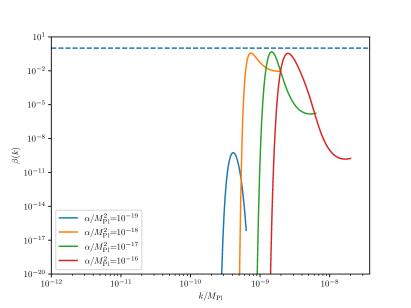
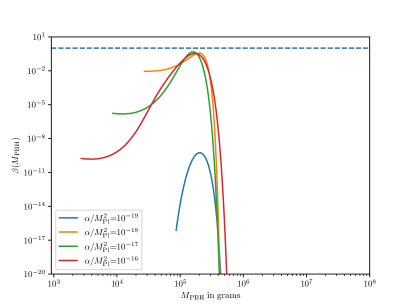
Figure 3: Left panel: The PBH mass function $\beta(k)$ as a function of the comoving number $k$ for different values of the $F(R)$ bouncing parameter $\alpha$. Right panel: The PBH mass function $\beta(M)$ as a function of the PBH mass $M_{\mathrm{PBH}}$ for different values of the $F(R)$ bouncing parameter $\alpha$. The blue dashed horizontal line stands for $\beta(M)=1$.

In the left panel of Fig. 3, we show how the PBH mass function changes with respect to the comoving scale $k$ for different values of the parameter $\alpha$. In particular, the mass function increases its overall amplitude as one increases the value of the parameter $\alpha$, a behavior which is kind of expected since as explained in Sec. V.1 by increasing $\alpha$ one starts to probe more and more smaller scales which become non-linear and can easily collapse to PBHs.

Interestingly, one can also notice that for values of $\alpha$ more or less larger than $10^{-19}M_{\scriptscriptstyle{\mathrm{Pl}}}^{2}$, the peak of the mass function saturates at a value close to $0.1$ independently of the value of $\alpha$. This behavior can be explained if one sees Fig. 2 where we see that for $\alpha>10^{-19}M_{\scriptscriptstyle{\mathrm{Pl}}}^{2}$, the curvature power spectrum enters gradually as we increase the value of $\alpha$ deep into the non perturbative regime where $P_{\zeta}(k)\gg 1$. Consequently, due to the effect of smoothing these enhanced perturbation modes do not contribute to the increase of the mass function as we go to high $k$ values. On the contrary, the overall effect of smoothing is to make the maximum amplitude of $\beta$ to saturate for $\alpha>10^{-19}M_{\scriptscriptstyle{\mathrm{Pl}}}^{2}$.

One can also infer a shift of the position of the peak of $\beta(k)$ towards the smaller scales, namely large $k$ values, a behavior which can be explained from the fact that $k_{\mathrm{max}}\sim\mathchoice{{\hbox{$\displaystyle\sqrt{\alpha\,}$}\lower 0.4pt\hbox{\vrule height=4.30554pt,depth=-3.44446pt}}}{{\hbox{$\textstyle\sqrt{\alpha\,}$}\lower 0.4pt\hbox{\vrule height=4.30554pt,depth=-3.44446pt}}}{{\hbox{$\scriptstyle\sqrt{\alpha\,}$}\lower 0.4pt\hbox{\vrule height=3.01389pt,depth=-2.41113pt}}}{{\hbox{$\scriptscriptstyle\sqrt{\alpha\,}$}\lower 0.4pt\hbox{\vrule height=2.15277pt,depth=-1.72223pt}}}$ [See Eq. (31) ].

Additionally, we witness as well a slight increase on the large $k$ region. This slight increase is due to the fact that in the high $k$ region where $\delta$ is very large, the PBH mass function (48) scales as $\beta(M)\propto 1/\sigma^{6}$ with $\sigma^{2}$ being suppressed on the very small PBH scales due to the effect of smoothing which becomes very important on these scales. As a consequence, at a scale around $k_{*}\sim k_{\mathrm{max}}/4$ all $\beta(k)$ curves start to slightly increase as one probes smaller scale modes $k$. [See the discussion in Appendix B.]

In the right panel of Fig. 3, we show how the $\beta$ function changes with respect to the PBH mass by varying the parameter $\alpha$. The observed behavior is similar as in the left panel of Fig. 3 with the only difference that now the position of the peak of $\beta(M)$ is more or less constant, independent of the value of $\alpha$. This can be understood if we see how the PBH mass scales with $\alpha$ and $k$. In particular, by defining the PBH mass being roughly equal to the mass within the horizon at horizon crossing time during the RD era one obtains that

$$M_{\mathrm{PBH}}\simeq M_{\mathrm{H}}=\frac{4\pi M_{\scriptscriptstyle{\mathrm{Pl}}}^{2}}{H}=\frac{8\pi M_{\scriptscriptstyle{\mathrm{Pl}}}^{2}\mathchoice{{\hbox{$\displaystyle\sqrt{\alpha\,}$}\lower 0.4pt\hbox{\vrule height=4.30554pt,depth=-3.44446pt}}}{{\hbox{$\textstyle\sqrt{\alpha\,}$}\lower 0.4pt\hbox{\vrule height=4.30554pt,depth=-3.44446pt}}}{{\hbox{$\scriptstyle\sqrt{\alpha\,}$}\lower 0.4pt\hbox{\vrule height=3.01389pt,depth=-2.41113pt}}}{{\hbox{$\scriptscriptstyle\sqrt{\alpha\,}$}\lower 0.4pt\hbox{\vrule height=2.15277pt,depth=-1.72223pt}}}}{k^{2}},$$ (51)

where in the last step we used Eq. (29) as well as the fact that during the RD era $H=1/(2t)$. Thus, despite the fact that as one increases the value of $\alpha$ the position of the peak of the $\beta$ function shifts to higher values of $k$, i.e. smaller scales [See left panel of Fig. 3] when one plots $\beta$ in terms of $M_{\mathrm{PBH}}$ the position of the peak of $\beta$ will shift to larger masses, since $M_{\mathrm{PBH}}\sim\mathchoice{{\hbox{$\displaystyle\sqrt{\alpha\,}$}\lower 0.4pt\hbox{\vrule height=4.30554pt,depth=-3.44446pt}}}{{\hbox{$\textstyle\sqrt{\alpha\,}$}\lower 0.4pt\hbox{\vrule height=4.30554pt,depth=-3.44446pt}}}{{\hbox{$\scriptstyle\sqrt{\alpha\,}$}\lower 0.4pt\hbox{\vrule height=3.01389pt,depth=-2.41113pt}}}{{\hbox{$\scriptscriptstyle\sqrt{\alpha\,}$}\lower 0.4pt\hbox{\vrule height=2.15277pt,depth=-1.72223pt}}}/k^{2}$ as it can be seen by Eq. (51). At the end, the overall effect is that the position of the peak of the function $\beta(M_{\mathrm{PBH}})$ is more or less constant independently of the value of $\alpha$.

At this point, it is useful to stress that the PBH masses produced substantially by the $F(R)$ gravity bouncing model studied here are very small, namely less than $10^{9}\mathrm{g}$, evaporating very quickly before the BBN time. One question one could ask is if with this bouncing model one can produce higher PBH masses, close to the solar mass as the ones probed by LIGO/VIRGO gravitational-wave detectors. To give an order of magnitude of the value that the $F(R)$ gravity parameter $\alpha$ should have in order to produce PBH masses of the order of $1M_{\odot}$ we can simply set in Eq. (51) $M_{\mathrm{PBH}}=1M_{\odot}$ and the comoving value $k$ equal to its maximum value, namely $k=k_{\mathrm{max}}=2\mathchoice{{\hbox{$\displaystyle\sqrt{\alpha\,}$}\lower 0.4pt\hbox{\vrule height=4.30554pt,depth=-3.44446pt}}}{{\hbox{$\textstyle\sqrt{\alpha\,}$}\lower 0.4pt\hbox{\vrule height=4.30554pt,depth=-3.44446pt}}}{{\hbox{$\scriptstyle\sqrt{\alpha\,}$}\lower 0.4pt\hbox{\vrule height=3.01389pt,depth=-2.41113pt}}}{{\hbox{$\scriptscriptstyle\sqrt{\alpha\,}$}\lower 0.4pt\hbox{\vrule height=2.15277pt,depth=-1.72223pt}}}$. At the end, one gets straightforwardly that

$$M_{\mathrm{PBH}}>M_{\odot}\Leftrightarrow\alpha<4\times 10^{-72}M_{\scriptscriptstyle{\mathrm{Pl}}}^{2}.$$ (52)

For such very small values of $\alpha$ the PBH mass function is dramatically suppressed as one may speculate by looking at the decreasing tendency of $\beta$ by decreasing the value of the parameter $\alpha$ in Fig. 3.

V.3 Constraining $\alpha$

We can now proceed to perform a full parameter-space analysis by calculating the PBH abundance at formation time $\Omega_{\mathrm{PBH,f}}$, for a wide range of values of the $F(R)$ parameter $\alpha$. In Fig. 4 we show how $\Omega_{\mathrm{PBH,f}}$ varies as a function of the bouncing parameter $\alpha$. In particular, we find that as $\alpha$ increases, the PBH abundance increases as well, as it can been speculated from Fig. 3. This behavior can be explained from the fact that as $\alpha$ increases the curvature power spectrum shifts to smaller and smaller scales widening in this way the range of modes $k$ which can potentially collapse to PBHs, hence enhancing the PBH mass function. Interestingly, we find that for values $\alpha\geq 10^{-19}M_{\scriptscriptstyle{\mathrm{Pl}}}^{2}$, $\Omega_{\mathrm{PBH,f}}$ saturates to a plateau which is related with the saturation of the amplitude of the PBH mass function due to the effect of smoothing becoming more and more important as $\alpha$ increases [See the discussion in Sec. V.2.].

At the end, accounting for the fact that the masses of the formed PBHs are so small they evaporate very quickly after their formation. Consequently, the only natural condition which needs to be fulfilled so as to set constraints on the parameter $\alpha$ is that $\Omega_{\mathrm{PBH,f}}<1$. However, as recently noted in Papanikolaou:2020qtd such small PBHs evaporating before BBN can dominate the energy budget of the Universe and induce at second order in cosmological perturbation theory a GW background which can be detectable by future GW experiments. Requiring therefore that GWs are not overproduced during this early PBH dominated era, one can set constraints on the parameters of the PBH production mechanism and in our case the $F(R)$ gravity parameter $\alpha$. For the case of monochromatic PBH distributions one can show that in order for the GWs not to be overproduced one should require that  Papanikolaou:2020qtd

$$\Omega_{\mathrm{PBH,f}}<10^{-4}\left(10^{9}\mathrm{g}/M_{\mathrm{PBH}}\right)^{1/4}.$$ (53)

In our case, we have a broad PBH mass spectrum but given the fact that the position of the peak of the maximum of the PBH mass function depends slightly on the value of the parameter $\alpha$ we can use as a first approximation Eq. (53) in order to constrain the bouncing parameter $\alpha$. In order to be more precise, one should account for the full broad PBH mass distribution and compute the GW signal today accounting as well for the transition between the early PBH dominated era to the RD era Papanikolaou:2022chm , a study which goes beyond the scope of the present work and which we leave for a future project.

Thus, taking $M_{\mathrm{PBH}}\simeq 2\times 10^{5}\mathrm{g}$ which is more or less the PBH mass at the peak of the $\beta$ function one gets that $\Omega_{\mathrm{PBH,f}}<10^{-3}$. At the end, requiring this condition one finds numerically [See Fig. 4] that $\alpha$ should lie within the following range:

$$\alpha\leq 10^{-19}M^{2}_{\mathrm{Pl}}.$$ (54)

This constraint can be translated to constraints on the energy scale at the onset of the HBB phase $H_{\mathrm{RD}}$ given the fact that $t_{\mathrm{RD}}=1/\mathchoice{{\hbox{$\displaystyle\sqrt{\alpha\,}$}\lower 0.4pt\hbox{\vrule height=4.30554pt,depth=-3.44446pt}}}{{\hbox{$\textstyle\sqrt{\alpha\,}$}\lower 0.4pt\hbox{\vrule height=4.30554pt,depth=-3.44446pt}}}{{\hbox{$\scriptstyle\sqrt{\alpha\,}$}\lower 0.4pt\hbox{\vrule height=3.01389pt,depth=-2.41113pt}}}{{\hbox{$\scriptscriptstyle\sqrt{\alpha\,}$}\lower 0.4pt\hbox{\vrule height=2.15277pt,depth=-1.72223pt}}}$ and $H_{\mathrm{RD}}=1/(2t_{\mathrm{RD}})$. At the end, one can find that $H_{\mathrm{RD}}=\mathchoice{{\hbox{$\displaystyle\sqrt{\alpha\,}$}\lower 0.4pt\hbox{\vrule height=4.30554pt,depth=-3.44446pt}}}{{\hbox{$\textstyle\sqrt{\alpha\,}$}\lower 0.4pt\hbox{\vrule height=4.30554pt,depth=-3.44446pt}}}{{\hbox{$\scriptstyle\sqrt{\alpha\,}$}\lower 0.4pt\hbox{\vrule height=3.01389pt,depth=-2.41113pt}}}{{\hbox{$\scriptscriptstyle\sqrt{\alpha\,}$}\lower 0.4pt\hbox{\vrule height=2.15277pt,depth=-1.72223pt}}}/2$ and should vary within the following range:

$$H_{\mathrm{RD}}\leq 10^{-10}M_{\mathrm{Pl}}.$$ (55)

At this point, it is very important to stress that the energy scale at the onset of the RD era, given by $H_{\mathrm{RD}}$, can also be viewed as the lowest bound on the energy scale of the Universe at the bounce.

Figure 4: The PBH abundance at formation time $\Omega_{\mathrm{PBH,f}}$ as a function of the $F(R)$ bouncing parameter $\alpha$.

VI Conclusions

The non-singular bouncing cosmological paradigm is one of the most appealing alternatives to inflation. Since the bounce realization requires the violation of the null energy condition, it can be typically implemented in the framework of modified gravity. On the other hand, the phenomenology of PBH physics, and the associated PBH abundance constraints which span a range of masses over more than $50$ orders of magnitude, has recently started to be investigated in detail, since it can be used in order to probe and extract constraints on the early-universe behavior. Hence, studying PBHs both at inflationary and bounce scenarios, could be helpful to constrain such scenarions and extract possible distinguishable features.

In this work, we focused on the bounce realization within $F(R)$ modified gravity and we investigated the corresponding PBH phenomenology. By introducing an $F(R)$ gravity exotic phase close to the bounce compatible with a bouncing scale factor we studied its effect on the mass function of PBHs which form during the standard RD era described quite well within classical GR gravity. In particular, we calculated the curvature power spectrum at horizon crossing time, during the RD era, as a function of the the bounce parameter $\alpha$, which is actually the involved $F(R)$ gravity parameter.

Followingly, we calculated the PBH abundance in the context of peak theory, considering the non-linear relation between $\delta$ and $\zeta$ as well as the critical collapse law for the PBH masses. At the end, in Fig. 3 we showed how the PBH mass function changes by varying the bouncing parameter $\alpha$.

Additionally, by making a full parameter-space analysis, in Fig. 4 we gave the PBH abundance at formation time $\Omega_{\mathrm{PBH,f}}$ as a function of the bouncing parameter $\alpha$. Interestingly enough, we found that in order to avoid GW overproduction from an early PBH domination era before BBN, $\alpha$ should lie within the range $\alpha\leq 10^{-19}M^{2}_{\mathrm{Pl}}$. This constraint can be transformed to a constraint on the energy scale at the onset of the HBB phase $H_{\mathrm{RD}}\sim\mathchoice{{\hbox{$\displaystyle\sqrt{\alpha\,}$}\lower 0.4pt\hbox{\vrule height=4.30554pt,depth=-3.44446pt}}}{{\hbox{$\textstyle\sqrt{\alpha\,}$}\lower 0.4pt\hbox{\vrule height=4.30554pt,depth=-3.44446pt}}}{{\hbox{$\scriptstyle\sqrt{\alpha\,}$}\lower 0.4pt\hbox{\vrule height=3.01389pt,depth=-2.41113pt}}}{{\hbox{$\scriptscriptstyle\sqrt{\alpha\,}$}\lower 0.4pt\hbox{\vrule height=2.15277pt,depth=-1.72223pt}}}/2$ which can be recast as $H_{\mathrm{RD}}\leq 10^{-10}M_{\mathrm{Pl}}$.

We mention that the explored parameter space can be further constrained by evolving the PBH abundance $\Omega_{\mathrm{PBH}}$ up to later times, and accounting for current observational constraints on $\Omega_{\mathrm{PBH}}$ Carr:2020gox . Moreover, one can extract more stringent constraints by studying additionally the scalar induced stochastic gravitational-wave background (SGWB) associated to the primordial curvature perturbations which gave rise to PBHs (see Domenech:2021ztg for a review), as well as the SGWB induced from PBH Poisson fluctuations Papanikolaou:2020qtd ; Papanikolaou:2021uhe ; Papanikolaou:2022hkg ; Papanikolaou:2022chm .

Since PBH formation within bouncing cosmologies may serve as a novel tool to study alternative theories of gravity, one should perform a similar analysis in other modified gravity scenarios, and examine whether there are qualitative and quantitative differences amongst them. In particular, one can extend our formalism by accounting as well for the effect of modified gravity on the background and perturbation evolution during the period of PBH formation generalising in a sense the peak theory formalism and investigating the full gravitational collapse dynamics in modified gravity setups. Such a detailed investigation is beyond the scope of this paper and can be be performed elsewhere.

Appendix A Investigating different bouncing scale factor parametrisations

Up to now, we have considered that the scale factor close to the bounce is parametrized by (5), by keeping terms up to quadratic order in $t$ in the Taylor expansion for $a(t)$. Thus, a legitimate question to ask is how our results will change by changing the scale factor parametrisation near the bounce. In general, the scale factor near a non-singular bounce can be parameterized as Odintsov:2020zct

$$a_{\mathrm{b}}(t)\simeq(1+\alpha t^{2})^{n},$$ (56)

where $n$ is a real number. In the following we study the cases where $n=2$ and $n=3$ and we examine how the curvature power spectrum changes accordingly.

1) $a(t)=(1+\alpha t^{2})^{2}$:

Using this parametrisation for the scale factor near the bounce, and solving Eq. (3) for $F(R)$ we find that

$$F_{b}(R(t)) =\frac{1}{420}t^{2}\alpha^{2}\Big{(}99225+t^{2}\alpha\Big{(}-814275+$$ (57)

$$t^{2}\alpha\Big{(}91875+t^{2}\alpha\Big{(}15855+t^{2}\alpha\Big{(}3360+t^{2}\alpha\Big{(}245$$

$$+t^{2}\alpha[75+t^{2}\alpha(-25+t^{2}\alpha)]\Big{)}\Big{)}\Big{)}\Big{)}\Big{)}\Big{)}$$

$$+\frac{1}{\alpha^{5}}(105+t^{2}\alpha(525+t^{2}\alpha(-1050+t^{2}\alpha[350$$

$$+t^{2}\alpha(-35+t^{2}\alpha)])))C+\frac{1}{8\mathchoice{{\hbox{$\displaystyle\sqrt{t^{2}\alpha\,}$}\lower 0.4pt\hbox{\vrule height=7.95523pt,depth=-6.36421pt}}}{{\hbox{$\textstyle\sqrt{t^{2}\alpha\,}$}\lower 0.4pt\hbox{\vrule height=7.95523pt,depth=-6.36421pt}}}{{\hbox{$\scriptstyle\sqrt{t^{2}\alpha\,}$}\lower 0.4pt\hbox{\vrule height=5.59444pt,depth=-4.47557pt}}}{{\hbox{$\scriptscriptstyle\sqrt{t^{2}\alpha\,}$}\lower 0.4pt\hbox{\vrule height=4.36427pt,depth=-3.49144pt}}}}9\pi t\alpha^{3/2}(105$$

$$+t^{2}\alpha(525+t^{2}\alpha(-1050+t^{2}\alpha[350+t^{2}\alpha(-35$$

$$+t^{2}\alpha)])))\cdot\mathrm{Erfc}(t\mathchoice{{\hbox{$\displaystyle\sqrt{t\alpha\,}$}\lower 0.4pt\hbox{\vrule height=6.15079pt,depth=-4.92065pt}}}{{\hbox{$\textstyle\sqrt{t\alpha\,}$}\lower 0.4pt\hbox{\vrule height=6.15079pt,depth=-4.92065pt}}}{{\hbox{$\scriptstyle\sqrt{t\alpha\,}$}\lower 0.4pt\hbox{\vrule height=4.30556pt,depth=-3.44447pt}}}{{\hbox{$\scriptscriptstyle\sqrt{t\alpha\,}$}\lower 0.4pt\hbox{\vrule height=3.0754pt,depth=-2.46033pt}}}/\mathchoice{{\hbox{$\displaystyle\sqrt{2\,}$}\lower 0.4pt\hbox{\vrule height=6.44444pt,depth=-5.15558pt}}}{{\hbox{$\textstyle\sqrt{2\,}$}\lower 0.4pt\hbox{\vrule height=6.44444pt,depth=-5.15558pt}}}{{\hbox{$\scriptstyle\sqrt{2\,}$}\lower 0.4pt\hbox{\vrule height=4.51111pt,depth=-3.6089pt}}}{{\hbox{$\scriptscriptstyle\sqrt{2\,}$}\lower 0.4pt\hbox{\vrule height=3.22221pt,depth=-2.57779pt}}})\mathrm{Erfi}(t\mathchoice{{\hbox{$\displaystyle\sqrt{t\alpha\,}$}\lower 0.4pt\hbox{\vrule height=6.15079pt,depth=-4.92065pt}}}{{\hbox{$\textstyle\sqrt{t\alpha\,}$}\lower 0.4pt\hbox{\vrule height=6.15079pt,depth=-4.92065pt}}}{{\hbox{$\scriptstyle\sqrt{t\alpha\,}$}\lower 0.4pt\hbox{\vrule height=4.30556pt,depth=-3.44447pt}}}{{\hbox{$\scriptscriptstyle\sqrt{t\alpha\,}$}\lower 0.4pt\hbox{\vrule height=3.0754pt,depth=-2.46033pt}}}/\mathchoice{{\hbox{$\displaystyle\sqrt{2\,}$}\lower 0.4pt\hbox{\vrule height=6.44444pt,depth=-5.15558pt}}}{{\hbox{$\textstyle\sqrt{2\,}$}\lower 0.4pt\hbox{\vrule height=6.44444pt,depth=-5.15558pt}}}{{\hbox{$\scriptstyle\sqrt{2\,}$}\lower 0.4pt\hbox{\vrule height=4.51111pt,depth=-3.6089pt}}}{{\hbox{$\scriptscriptstyle\sqrt{2\,}$}\lower 0.4pt\hbox{\vrule height=3.22221pt,depth=-2.57779pt}}})$$

$$+\frac{9}{8}\alpha(-e^{t^{2}\alpha/2}\mathchoice{{\hbox{$\displaystyle\sqrt{2\pi\,}$}\lower 0.4pt\hbox{\vrule height=6.44444pt,depth=-5.15558pt}}}{{\hbox{$\textstyle\sqrt{2\pi\,}$}\lower 0.4pt\hbox{\vrule height=6.44444pt,depth=-5.15558pt}}}{{\hbox{$\scriptstyle\sqrt{2\pi\,}$}\lower 0.4pt\hbox{\vrule height=4.51111pt,depth=-3.6089pt}}}{{\hbox{$\scriptscriptstyle\sqrt{2\pi\,}$}\lower 0.4pt\hbox{\vrule height=3.22221pt,depth=-2.57779pt}}}t\mathchoice{{\hbox{$\displaystyle\sqrt{\alpha\,}$}\lower 0.4pt\hbox{\vrule height=4.30554pt,depth=-3.44446pt}}}{{\hbox{$\textstyle\sqrt{\alpha\,}$}\lower 0.4pt\hbox{\vrule height=4.30554pt,depth=-3.44446pt}}}{{\hbox{$\scriptstyle\sqrt{\alpha\,}$}\lower 0.4pt\hbox{\vrule height=3.01389pt,depth=-2.41113pt}}}{{\hbox{$\scriptscriptstyle\sqrt{\alpha\,}$}\lower 0.4pt\hbox{\vrule height=2.15277pt,depth=-1.72223pt}}}(105+t^{2}\alpha(-790$$

$$+t^{2}\alpha[318+t^{2}\alpha(-34+t^{2}\alpha)]))+\pi(105+t^{2}\alpha$$

$$(525+t^{2}\alpha(-1050+t^{2}\alpha[350+t^{2}\alpha(-35+t^{2}\alpha)$$

$$])))\cdot\mathrm{Erfi}(t\mathchoice{{\hbox{$\displaystyle\sqrt{t\alpha\,}$}\lower 0.4pt\hbox{\vrule height=6.15079pt,depth=-4.92065pt}}}{{\hbox{$\textstyle\sqrt{t\alpha\,}$}\lower 0.4pt\hbox{\vrule height=6.15079pt,depth=-4.92065pt}}}{{\hbox{$\scriptstyle\sqrt{t\alpha\,}$}\lower 0.4pt\hbox{\vrule height=4.30556pt,depth=-3.44447pt}}}{{\hbox{$\scriptscriptstyle\sqrt{t\alpha\,}$}\lower 0.4pt\hbox{\vrule height=3.0754pt,depth=-2.46033pt}}}/\mathchoice{{\hbox{$\displaystyle\sqrt{2\,}$}\lower 0.4pt\hbox{\vrule height=6.44444pt,depth=-5.15558pt}}}{{\hbox{$\textstyle\sqrt{2\,}$}\lower 0.4pt\hbox{\vrule height=6.44444pt,depth=-5.15558pt}}}{{\hbox{$\scriptstyle\sqrt{2\,}$}\lower 0.4pt\hbox{\vrule height=4.51111pt,depth=-3.6089pt}}}{{\hbox{$\scriptscriptstyle\sqrt{2\,}$}\lower 0.4pt\hbox{\vrule height=3.22221pt,depth=-2.57779pt}}}))\mathrm{Erf}(t\mathchoice{{\hbox{$\displaystyle\sqrt{t\alpha\,}$}\lower 0.4pt\hbox{\vrule height=6.15079pt,depth=-4.92065pt}}}{{\hbox{$\textstyle\sqrt{t\alpha\,}$}\lower 0.4pt\hbox{\vrule height=6.15079pt,depth=-4.92065pt}}}{{\hbox{$\scriptstyle\sqrt{t\alpha\,}$}\lower 0.4pt\hbox{\vrule height=4.30556pt,depth=-3.44447pt}}}{{\hbox{$\scriptscriptstyle\sqrt{t\alpha\,}$}\lower 0.4pt\hbox{\vrule height=3.0754pt,depth=-2.46033pt}}}/\mathchoice{{\hbox{$\displaystyle\sqrt{2\,}$}\lower 0.4pt\hbox{\vrule height=6.44444pt,depth=-5.15558pt}}}{{\hbox{$\textstyle\sqrt{2\,}$}\lower 0.4pt\hbox{\vrule height=6.44444pt,depth=-5.15558pt}}}{{\hbox{$\scriptstyle\sqrt{2\,}$}\lower 0.4pt\hbox{\vrule height=4.51111pt,depth=-3.6089pt}}}{{\hbox{$\scriptscriptstyle\sqrt{2\,}$}\lower 0.4pt\hbox{\vrule height=3.22221pt,depth=-2.57779pt}}})$$

$$-\frac{1}{840}e^{t^{2}\alpha/2}t^{12}\alpha^{7}(105+t^{2}\alpha(-790+t^{2}\alpha[318$$

$$+t^{2}\alpha(-34+t^{2}\alpha)]))\mathrm{ExpIntE}(-\frac{9}{2},\frac{t^{2}\alpha}{2}),$$

where $\mathrm{ExpIntE}$ is the exponential integral function $E_{n}(z)$.

Similar to the previous case, keeping terms up to $\mathcal{O}(\alpha t^{2})$ the expression for $z(t)$ becomes

$$z(t)=U+Vt-Xt^{2},$$ (58)

where

$$U=\frac{\mathchoice{{\hbox{$\displaystyle\sqrt{105\,}$}\lower 0.4pt\hbox{\vrule height=6.44444pt,depth=-5.15558pt}}}{{\hbox{$\textstyle\sqrt{105\,}$}\lower 0.4pt\hbox{\vrule height=6.44444pt,depth=-5.15558pt}}}{{\hbox{$\scriptstyle\sqrt{105\,}$}\lower 0.4pt\hbox{\vrule height=4.51111pt,depth=-3.6089pt}}}{{\hbox{$\scriptscriptstyle\sqrt{105\,}$}\lower 0.4pt\hbox{\vrule height=3.22221pt,depth=-2.57779pt}}}\alpha}{2\alpha\kappa\mathchoice{{\hbox{$\displaystyle\sqrt{\alpha^{7}/C\,}$}\lower 0.4pt\hbox{\vrule height=7.5pt,depth=-6.00003pt}}}{{\hbox{$\textstyle\sqrt{\alpha^{7}/C\,}$}\lower 0.4pt\hbox{\vrule height=7.5pt,depth=-6.00003pt}}}{{\hbox{$\scriptstyle\sqrt{\alpha^{7}/C\,}$}\lower 0.4pt\hbox{\vrule height=5.25pt,depth=-4.20003pt}}}{{\hbox{$\scriptscriptstyle\sqrt{\alpha^{7}/C\,}$}\lower 0.4pt\hbox{\vrule height=3.75pt,depth=-3.00002pt}}}},$$ (59)

$$V=\frac{\mathchoice{{\hbox{$\displaystyle\sqrt{\alpha^{7}/C\,}$}\lower 0.4pt\hbox{\vrule height=7.5pt,depth=-6.00003pt}}}{{\hbox{$\textstyle\sqrt{\alpha^{7}/C\,}$}\lower 0.4pt\hbox{\vrule height=7.5pt,depth=-6.00003pt}}}{{\hbox{$\scriptstyle\sqrt{\alpha^{7}/C\,}$}\lower 0.4pt\hbox{\vrule height=5.25pt,depth=-4.20003pt}}}{{\hbox{$\scriptscriptstyle\sqrt{\alpha^{7}/C\,}$}\lower 0.4pt\hbox{\vrule height=3.75pt,depth=-3.00002pt}}}(2592\pi\alpha^{12}-1225C^{2})}{12\alpha^{12}\kappa\mathchoice{{\hbox{$\displaystyle\sqrt{210\pi\,}$}\lower 0.4pt\hbox{\vrule height=6.44444pt,depth=-5.15558pt}}}{{\hbox{$\textstyle\sqrt{210\pi\,}$}\lower 0.4pt\hbox{\vrule height=6.44444pt,depth=-5.15558pt}}}{{\hbox{$\scriptstyle\sqrt{210\pi\,}$}\lower 0.4pt\hbox{\vrule height=4.51111pt,depth=-3.6089pt}}}{{\hbox{$\scriptscriptstyle\sqrt{210\pi\,}$}\lower 0.4pt\hbox{\vrule height=3.22221pt,depth=-2.57779pt}}}},$$ (60)

$$X =\frac{(\alpha^{7}/C)^{3/2}}{1890\alpha^{18}\kappa\pi\mathchoice{{\hbox{$\displaystyle\sqrt{105\,}$}\lower 0.4pt\hbox{\vrule height=6.44444pt,depth=-5.15558pt}}}{{\hbox{$\textstyle\sqrt{105\,}$}\lower 0.4pt\hbox{\vrule height=6.44444pt,depth=-5.15558pt}}}{{\hbox{$\scriptstyle\sqrt{105\,}$}\lower 0.4pt\hbox{\vrule height=4.51111pt,depth=-3.6089pt}}}{{\hbox{$\scriptscriptstyle\sqrt{105\,}$}\lower 0.4pt\hbox{\vrule height=3.22221pt,depth=-2.57779pt}}}}\bigl{[}419904\pi^{2}\alpha^{18}+45360\pi\alpha^{12}C$$

$$+1190700\pi\alpha^{6}C^{2}+42875C^{3}\bigr{]}.$$ (61)

Thus, evaluating the curvature perturbation near the bounce, at leading order in $t$, we obtain

$$\zeta_{k} =C_{1}(k)H\bigg{[}\frac{k^{2}U^{2}}{2V^{2}+4UX-4U^{2}\alpha},$$

$$\frac{-UV+tV^{2}+2tUX-2tU^{2}\alpha}{U\mathchoice{{\hbox{$\displaystyle\sqrt{V^{2}+2U(X-U\alpha)\,}$}\lower 0.4pt\hbox{\vrule height=8.63776pt,depth=-6.91023pt}}}{{\hbox{$\textstyle\sqrt{V^{2}+2U(X-U\alpha)\,}$}\lower 0.4pt\hbox{\vrule height=8.63776pt,depth=-6.91023pt}}}{{\hbox{$\scriptstyle\sqrt{V^{2}+2U(X-U\alpha)\,}$}\lower 0.4pt\hbox{\vrule height=6.0722pt,depth=-4.85779pt}}}{{\hbox{$\scriptscriptstyle\sqrt{V^{2}+2U(X-U\alpha)\,}$}\lower 0.4pt\hbox{\vrule height=4.70554pt,depth=-3.76445pt}}}}\bigg{]}$$ (62)

$$+C_{2}(k)~{}{}_{1}F_{1}\bigg{\{}-\frac{k^{2}U^{2}}{4[V^{2}+2U(X-U\alpha)]},\frac{1}{2},$$

$$\frac{[-tV^{2}+U(V-2tX)+2tU^{2}\alpha]^{2}}{U^{2}[V^{2}+2U(X-U\alpha)]}\bigg{\}}.$$

The forms of $C_{1}(k)$ and $C_{2}(k)$ are determined using the initial conditions given in (24) modified appropriately for the present case where $a(t)=(1+\alpha t^{2})^{2}.$

Below, we show the curvature power spectrum $\mathcal{P}_{\zeta}(k)=k^{3}|\zeta_{k}|^{2}/(2\pi^{2})$ by varying the $F(R)$ bouncing parameter $\alpha$. As one may notice from the left panel of Fig. 5 in the case where $n=2$, $\mathcal{P}_{\zeta}(k)$ becomes very sensitive with $\alpha$ with a general tendency to increase on small scales, i.e. large $k$ values, probing gradually the non linear regime. In addition, it is worth highlighting the fact that independently of the value of $\alpha$ $\mathcal{P}_{\zeta}(k)$ increases very abruptly to large values within less than one order of magnitude in $k$ signalling the fact that in contrast with the $n=1$, one is met with an almost monochromatic curvature power spectrum giving rise to PBHs.

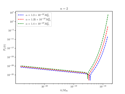
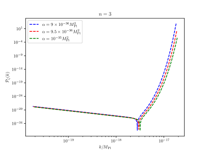
Figure 5: The curvature power spectrum $\mathcal{P}_{\zeta}(k)$ for different values of $\alpha$ for $n=2$ and $n=3$.

2) $a(t)=(1+\alpha t^{2})^{3}$:

With the same reasoning as before, the solution for $F(R)$ around the bounce reads as

$$F_{b}(t) =6\alpha+324\alpha^{2}t^{2}+\Big{[}324t^{4}\alpha^{3}(-3+t^{2}\alpha)$$ (63)

$$-\frac{54}{288}e^{\frac{3t^{2}\alpha}{2}}t\alpha^{2}\left[1+t^{2}\alpha(-8+3t^{2}\alpha)\right]C$$

$$+9C\mathchoice{{\hbox{$\displaystyle\sqrt{6\pi\,}$}\lower 0.4pt\hbox{\vrule height=6.44444pt,depth=-5.15558pt}}}{{\hbox{$\textstyle\sqrt{6\pi\,}$}\lower 0.4pt\hbox{\vrule height=6.44444pt,depth=-5.15558pt}}}{{\hbox{$\scriptstyle\sqrt{6\pi\,}$}\lower 0.4pt\hbox{\vrule height=4.51111pt,depth=-3.6089pt}}}{{\hbox{$\scriptscriptstyle\sqrt{6\pi\,}$}\lower 0.4pt\hbox{\vrule height=3.22221pt,depth=-2.57779pt}}}\alpha^{9/2}(1+9t^{2}\alpha[1+t^{2}\alpha(-3$$

$$+t^{2}\alpha)])\mathrm{Erfi}\left(\mathchoice{{\hbox{$\displaystyle\sqrt{\frac{3\alpha}{2}\,}$}\lower 0.4pt\hbox{\vrule height=9.66666pt,depth=-7.73337pt}}}{{\hbox{$\textstyle\sqrt{\frac{3\alpha}{2}\,}$}\lower 0.4pt\hbox{\vrule height=6.76666pt,depth=-5.41336pt}}}{{\hbox{$\scriptstyle\sqrt{\frac{3\alpha}{2}\,}$}\lower 0.4pt\hbox{\vrule height=4.83331pt,depth=-3.86667pt}}}{{\hbox{$\scriptscriptstyle\sqrt{\frac{3\alpha}{2}\,}$}\lower 0.4pt\hbox{\vrule height=4.83331pt,depth=-3.86667pt}}}t\right)\Big{]}.$$

Once again, keeping up to $\mathcal{O}(\alpha t^{2})$ terms in the scalar perturbation, we extract the form of $z(t)$ as

$$z(t)=U+Vt-Xt^{2},$$ (64)

where

$$U= \frac{\mathchoice{{\hbox{$\displaystyle\sqrt{6\,}$}\lower 0.4pt\hbox{\vrule height=6.44444pt,depth=-5.15558pt}}}{{\hbox{$\textstyle\sqrt{6\,}$}\lower 0.4pt\hbox{\vrule height=6.44444pt,depth=-5.15558pt}}}{{\hbox{$\scriptstyle\sqrt{6\,}$}\lower 0.4pt\hbox{\vrule height=4.51111pt,depth=-3.6089pt}}}{{\hbox{$\scriptscriptstyle\sqrt{6\,}$}\lower 0.4pt\hbox{\vrule height=3.22221pt,depth=-2.57779pt}}}}{\kappa},\quad V=\frac{(-124416+\alpha C^{2})}{24\mathchoice{{\hbox{$\displaystyle\sqrt{6\,}$}\lower 0.4pt\hbox{\vrule height=6.44444pt,depth=-5.15558pt}}}{{\hbox{$\textstyle\sqrt{6\,}$}\lower 0.4pt\hbox{\vrule height=6.44444pt,depth=-5.15558pt}}}{{\hbox{$\scriptstyle\sqrt{6\,}$}\lower 0.4pt\hbox{\vrule height=4.51111pt,depth=-3.6089pt}}}{{\hbox{$\scriptscriptstyle\sqrt{6\,}$}\lower 0.4pt\hbox{\vrule height=3.22221pt,depth=-2.57779pt}}}\kappa C},$$ (65)

$$X= \frac{\alpha(746496+\alpha C^{2})}{6912(\mathchoice{{\hbox{$\displaystyle\sqrt{6\,}$}\lower 0.4pt\hbox{\vrule height=6.44444pt,depth=-5.15558pt}}}{{\hbox{$\textstyle\sqrt{6\,}$}\lower 0.4pt\hbox{\vrule height=6.44444pt,depth=-5.15558pt}}}{{\hbox{$\scriptstyle\sqrt{6\,}$}\lower 0.4pt\hbox{\vrule height=4.51111pt,depth=-3.6089pt}}}{{\hbox{$\scriptscriptstyle\sqrt{6\,}$}\lower 0.4pt\hbox{\vrule height=3.22221pt,depth=-2.57779pt}}}\kappa)}.$$ (66)

The corresponding solution for the curvature perturbation, at leading order in $t$, is

$$\zeta_{k} =C_{1}(k)H\bigg{[}\frac{k^{2}U^{2}}{2V^{2}+4UX-4U^{2}\alpha},$$

$$\frac{-UV+tV^{2}+2tUX-2tU^{2}\alpha}{U\mathchoice{{\hbox{$\displaystyle\sqrt{V^{2}+2U(X-U\alpha)\,}$}\lower 0.4pt\hbox{\vrule height=8.63776pt,depth=-6.91023pt}}}{{\hbox{$\textstyle\sqrt{V^{2}+2U(X-U\alpha)\,}$}\lower 0.4pt\hbox{\vrule height=8.63776pt,depth=-6.91023pt}}}{{\hbox{$\scriptstyle\sqrt{V^{2}+2U(X-U\alpha)\,}$}\lower 0.4pt\hbox{\vrule height=6.0722pt,depth=-4.85779pt}}}{{\hbox{$\scriptscriptstyle\sqrt{V^{2}+2U(X-U\alpha)\,}$}\lower 0.4pt\hbox{\vrule height=4.70554pt,depth=-3.76445pt}}}}\bigg{]}$$ (67)

$$+C_{2}(k)~{}{}_{1}F_{1}\bigg{\{}-\frac{k^{2}U^{2}}{4[V^{2}+2U(X-U\alpha)]},\frac{1}{2},$$

$$\frac{[-tV^{2}+U(V-2tX)+2tU^{2}\alpha]^{2}}{U^{2}[V^{2}+2U(X-U\alpha)]}\bigg{\}}.$$

In the right panel of Fig. 5 we show again the curvature power spectrum for the $n=3$ case by varying the parameter $\alpha$. In particular, as in the $n=2$, one can notice a power spectrum $\mathcal{P}_{\zeta}(k)$ with an amplitude quite sensitive to the variation of the $F(R)$ bouncing parameter $\alpha$ and with a tendency to lead to a monochromatic PBH mass distribution in contrast with the $n=1$ case.

Consequently, one can argue that our results are nearly the same for $(1+\alpha t^{2}),\ (1+\alpha t^{2})^{2},\ (1+\alpha t^{2})^{3}$ and other values of $n$ in $(1+\alpha t^{2})^{n}$ with $n>1$. In particular, in contrast with the $n=1$ case, we find a very sensitive behavior of the amplitude of $\mathcal{P}_{\zeta}(k)$ and a tendency of $\mathcal{P}_{\zeta}(k)$ to lead to a monochromatic PBH mass function.

Finally, one should comment on the order of masses produced within the parametrisations where $n>1$. In particular, as we can see fron Fig. 5 $k_{\mathrm{max}}\sim 10^{-18}M_{\scriptscriptstyle{\mathrm{Pl}}}$ and given the fact that $M_{\mathrm{PBH}}\propto\mathchoice{{\hbox{$\displaystyle\sqrt{\alpha\,}$}\lower 0.4pt\hbox{\vrule height=4.30554pt,depth=-3.44446pt}}}{{\hbox{$\textstyle\sqrt{\alpha\,}$}\lower 0.4pt\hbox{\vrule height=4.30554pt,depth=-3.44446pt}}}{{\hbox{$\scriptstyle\sqrt{\alpha\,}$}\lower 0.4pt\hbox{\vrule height=3.01389pt,depth=-2.41113pt}}}{{\hbox{$\scriptscriptstyle\sqrt{\alpha\,}$}\lower 0.4pt\hbox{\vrule height=2.15277pt,depth=-1.72223pt}}}/k^{2}$ one gets that for $\alpha\sim 10^{-36}M_{\scriptscriptstyle{\mathrm{Pl}}}^{2}$ $M_{\mathrm{PBH}}\sim 10^{13}\mathrm{g}\sim 10^{-20}M_{\odot}$ many orders of magnitude larger than the order of PBH masses produced in the $n=1$ case but still quite small compared to the PBH masses detected by the LIGO-VIRGO detectors which are of the order of the solar mass.

We mention here that other possible bouncing scale factor forms that have been studied in the literature are $\cosh\left(1+\alpha t^{2}\right)$ and $e^{\alpha t^{2}}$. However, when expanded around $t$ their forms become similar to $(1+\alpha t^{2})^{n}$, hence our above results become quite general, being valid for any parametrization of the scale factor giving rise to a bounce.

Appendix B The PBH mass function on small scales

We show below the smoothed power spectra $\sigma^{2}$ and $\mu^{2}$ with respect to the comoving scale $k$ by varying the $F(R)$ gravity parameter $\alpha$.

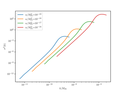
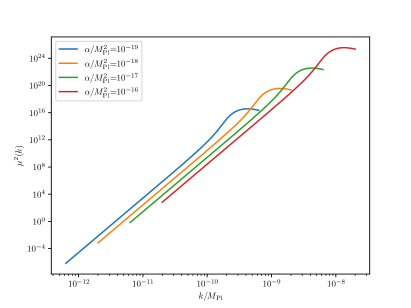
Figure 6: The smoothed power spectra $\sigma^{2}(k)$ and $\mu^{2}(k)$ as a function of $k$ for different values of $\alpha$.

Writing now the fraction of the Universe at a peak of height $\nu\equiv\delta/\sigma$, which will collapse to form a PBH [See Eq. (47)] as a function of the energy density contrast one can recast it as

$$\beta_{\delta}=\frac{\mathcal{K}}{4\pi^{2}}\left(\delta-\frac{3\delta^{2}}{8}-\delta_{\mathrm{c}}\right)^{\gamma}\delta^{3}e^{-\frac{\delta^{2}}{2\sigma^{2}}}\frac{\mu^{3}}{\sigma^{6}}.$$ (68)

At the end, after integrating the $\beta_{\delta}$ over $\delta$ one will have that $\beta(k)=H(\sigma)\mu^{3}(k)/\sigma^{6}(k)$ with the function $H(\sigma)$ being defined as

$$H(\sigma)\equiv\int_{\delta_{\mathrm{c,l-}}}^{4/3}\frac{\mathcal{K}}{4\pi^{2}}\left(\delta-\frac{3\delta^{2}}{8}-\delta_{\mathrm{c}}\right)^{\gamma}\delta^{3}e^{-\frac{\delta^{2}}{2\sigma^{2}}}$$ (69)

As it was checked numerically [See Fig. 8] for the range of $k$ values considered here $\delta/\sigma\ll 1$ and thus one can approximate $e^{-\frac{\delta^{2}}{2\sigma^{2}}}\simeq 1-\frac{\delta^{2}}{\sigma^{2}}$. As we decrease $\sigma$, $H(\sigma)$ decreases as well. However, due to the $1/\sigma^{6}$ dependence of $\beta$, as we approach the region close to $k_{\mathrm{max}}$, we see the slight increase in $\beta(k)$ as can be seen in Fig. 3. This region where one observes this slight increase of the $\beta$ function can be roughly defined as $k>k_{\mathrm{max}}/4=\mathchoice{{\hbox{$\displaystyle\sqrt{\alpha\,}$}\lower 0.4pt\hbox{\vrule height=4.30554pt,depth=-3.44446pt}}}{{\hbox{$\textstyle\sqrt{\alpha\,}$}\lower 0.4pt\hbox{\vrule height=4.30554pt,depth=-3.44446pt}}}{{\hbox{$\scriptstyle\sqrt{\alpha\,}$}\lower 0.4pt\hbox{\vrule height=3.01389pt,depth=-2.41113pt}}}{{\hbox{$\scriptscriptstyle\sqrt{\alpha\,}$}\lower 0.4pt\hbox{\vrule height=2.15277pt,depth=-1.72223pt}}}/2$.

Figure 7: The function $\mu^{3}(k)/\sigma^{6}(k)$ as a function of $k$ for different values of $\alpha$.

Figure 8: $\delta(k)/\sigma(k)$ as a function of $k$ for different values of $\alpha$.

References

- (1) A. A. Starobinsky, A New Type of Isotropic Cosmological Models Without Singularity, Phys. Lett. B91 (1980) 99–102.
- (2) A. H. Guth, The Inflationary Universe: A Possible Solution to the Horizon and Flatness Problems, Phys.Rev. D23 (1981) 347–356.
- (3) A. D. Linde, A New Inflationary Universe Scenario: A Possible Solution of the Horizon, Flatness, Homogeneity, Isotropy and Primordial Monopole Problems, Phys.Lett. B108 (1982) 389–393.
- (4) A. Albrecht and P. J. Steinhardt, Cosmology for Grand Unified Theories with Radiatively Induced Symmetry Breaking, Phys.Rev.Lett. 48 (1982) 1220–1223.
- (5) A. D. Linde, Chaotic Inflation, Phys.Lett. B129 (1983) 177–181.
- (6) A. Borde and A. Vilenkin, Singularities in inflationary cosmology: A Review, Int. J. Mod. Phys. D 5 (1996) 813–824, [gr-qc/9612036].
- (7) V. Mukhanov and R. Brandenberger, A nonsingular universe, Phys. Rev. Lett. 68 (Mar, 1992) 1969–1972.
- (8) R. H. Brandenberger, V. F. Mukhanov and A. Sornborger, A Cosmological theory without singularities, Phys. Rev. D 48 (1993) 1629–1642, [gr-qc/9303001].
- (9) M. Novello and S. E. P. Bergliaffa, Bouncing Cosmologies, Phys. Rept. 463 (2008) 127–213, [0802.1634].
- (10) M. Lilley and P. Peter, Bouncing alternatives to inflation, Comptes Rendus Physique 16 (2015) 1038–1047.
- (11) D. Battefeld and P. Peter, A Critical Review of Classical Bouncing Cosmologies, Phys. Rept. 571 (2015) 1–66, [1406.2790].
- (12) P. Peter and N. Pinto-Neto, Cosmology without inflation, Phys. Rev. D 78 (Sep, 2008) 063506.
- (13) CANTATA collaboration, E. N. Saridakis et al., Modified Gravity and Cosmology: An Update by the CANTATA Network, 2105.12582.
- (14) S. Nojiri and S. D. Odintsov, Introduction to modified gravity and gravitational alternative for dark energy, eConf C0602061 (2006) 06, [hep-th/0601213].
- (15) S. Capozziello and M. De Laurentis, Extended Theories of Gravity, Phys. Rept. 509 (2011) 167–321, [1108.6266].
- (16) D. Benisty, E. I. Guendelman, A. van de Venn, D. Vasak, J. Struckmeier and H. Stoecker, The dark side of the torsion: dark energy from propagating torsion, Eur. Phys. J. C 82 (2022) 264, [2109.01052].
- (17) D. Benisty, G. J. Olmo and D. Rubiera-Garcia, Singularity-Free and Cosmologically Viable Born-Infeld Gravity with Scalar Matter, Symmetry 13 (2021) 2108, [2103.15437].
- (18) G. Veneziano, Scale factor duality for classical and quantum strings, Phys. Lett. B 265 (1991) 287–294.
- (19) J. Khoury, B. A. Ovrut, P. J. Steinhardt and N. Turok, The Ekpyrotic universe: Colliding branes and the origin of the hot big bang, Phys. Rev. D 64 (2001) 123522, [hep-th/0103239].
- (20) J. Khoury, B. A. Ovrut, N. Seiberg, P. J. Steinhardt and N. Turok, From big crunch to big bang, Phys. Rev. D 65 (2002) 086007, [hep-th/0108187].
- (21) T. Biswas, A. Mazumdar and W. Siegel, Bouncing universes in string-inspired gravity, JCAP 03 (2006) 009, [hep-th/0508194].
- (22) S. Nojiri and E. N. Saridakis, Phantom without ghost, Astrophys. Space Sci. 347 (2013) 221–226, [1301.2686].
- (23) K. Bamba, A. N. Makarenko, A. N. Myagky, S. Nojiri and S. D. Odintsov, Bounce cosmology from gravity and bigravity, JCAP 01 (2014) 008, [1309.3748].
- (24) S. Nojiri and S. D. Odintsov, Mimetic gravity: inflation, dark energy and bounce, 1408.3561.
- (25) Y.-F. Cai, S.-H. Chen, J. B. Dent, S. Dutta and E. N. Saridakis, Matter Bounce Cosmology with the f(T) Gravity, Class. Quant. Grav. 28 (2011) 215011, [1104.4349].
- (26) Y. Shtanov and V. Sahni, Bouncing brane worlds, Phys. Lett. B 557 (2003) 1–6, [gr-qc/0208047].
- (27) E. N. Saridakis, Cyclic Universes from General Collisionless Braneworld Models, Nucl. Phys. B 808 (2009) 224–236, [0710.5269].
- (28) Y.-F. Cai and E. N. Saridakis, Non-singular cosmology in a model of non-relativistic gravity, JCAP 10 (2009) 020, [0906.1789].
- (29) E. N. Saridakis, Horava-Lifshitz Dark Energy, Eur. Phys. J. C 67 (2010) 229–235, [0905.3532].
- (30) Y.-F. Cai, C. Gao and E. N. Saridakis, Bounce and cyclic cosmology in extended nonlinear massive gravity, JCAP 10 (2012) 048, [1207.3786].
- (31) J.-L. Lehners, Ekpyrotic and Cyclic Cosmology, Phys. Rept. 465 (2008) 223–263, [0806.1245].
- (32) S. Banerjee and E. N. Saridakis, Bounce and cyclic cosmology in weakly broken galileon theories, Phys. Rev. D 95 (2017) 063523, [1604.06932].
- (33) E. N. Saridakis, S. Banerjee and R. Myrzakulov, Bounce and cyclic cosmology in new gravitational scalar-tensor theories, Phys. Rev. D 98 (2018) 063513, [1807.00346].
- (34) Y.-F. Cai, Exploring Bouncing Cosmologies with Cosmological Surveys, Sci. China Phys. Mech. Astron. 57 (2014) 1414–1430, [1405.1369].
- (35) Y.-F. Cai, J. Quintin, E. N. Saridakis and E. Wilson-Ewing, Nonsingular bouncing cosmologies in light of BICEP2, JCAP 07 (2014) 033, [1404.4364].
- (36) B. J. Carr, The Primordial black hole mass spectrum, Astrophys. J. 201 (1975) 1–19.
- (37) B. J. Carr, K. Kohri, Y. Sendouda and J. Yokoyama, New cosmological constraints on primordial black holes, Phys. Rev. D81 (2010) 104019, [0912.5297].
- (38) Y. B. Zel’dovich and I. D. Novikov, The Hypothesis of Cores Retarded during Expansion and the Hot Cosmological Model, Soviet Astronomy 10 (Feb., 1967) 602.
- (39) B. J. Carr and S. W. Hawking, Black holes in the early Universe, Mon. Not. Roy. Astron. Soc. 168 (1974) 399–415.
- (40) B. J. Carr, The primordial black hole mass spectrum, ApJ 201 (Oct., 1975) 1–19.
- (41) T. Harada, C.-M. Yoo and K. Kohri, Threshold of primordial black hole formation, Phys. Rev. D88 (2013) 084051, [1309.4201].
- (42) I. Musco, Threshold for primordial black holes: Dependence on the shape of the cosmological perturbations, Phys. Rev. D 100 (2019) 123524, [1809.02127].
- (43) A. Kehagias, I. Musco and A. Riotto, Non-Gaussian Formation of Primordial Black Holes: Effects on the Threshold, JCAP 12 (2019) 029, [1906.07135].
- (44) I. Musco, V. De Luca, G. Franciolini and A. Riotto, Threshold for primordial black holes. II. A simple analytic prescription, Phys. Rev. D 103 (2021) 063538, [2011.03014].
- (45) I. Musco and T. Papanikolaou, Primordial black hole formation for an anisotropic perfect fluid: initial conditions and estimation of the threshold, 2110.05982.
- (46) A. Addazi et al., Quantum gravity phenomenology at the dawn of the multi-messenger era—A review, Prog. Part. Nucl. Phys. 125 (2022) 103948, [2111.05659].
- (47) T. Papanikolaou, Towards the primordial black hole formation threshold in a time-dependent equation-of-state background, 2205.07748.
- (48) G. F. Chapline, Cosmological effects of primordial black holes, Nature 253 (1975) 251–252.
- (49) S. Clesse and J. García-Bellido, Seven Hints for Primordial Black Hole Dark Matter, Phys. Dark Univ. 22 (2018) 137–146, [1711.10458].
- (50) P. Meszaros, Primeval black holes and galaxy formation, Astron. Astrophys. 38 (1975) 5–13.
- (51) N. Afshordi, P. McDonald and D. Spergel, Primordial black holes as dark matter: The Power spectrum and evaporation of early structures, Astrophys. J. Lett. 594 (2003) L71–L74, [astro-ph/0302035].
- (52) B. J. Carr and M. J. Rees, How large were the first pregalactic objects?, Monthly Notices of Royal Astronomical Society 206 (Jan., 1984) 315–325.
- (53) R. Bean and J. Magueijo, Could supermassive black holes be quintessential primordial black holes?, Phys. Rev. D 66 (2002) 063505, [astro-ph/0204486].
- (54) T. Nakamura, M. Sasaki, T. Tanaka and K. S. Thorne, Gravitational waves from coalescing black hole MACHO binaries, Astrophys. J. 487 (1997) L139–L142, [astro-ph/9708060].
- (55) K. Ioka, T. Chiba, T. Tanaka and T. Nakamura, Black hole binary formation in the expanding universe: Three body problem approximation, Phys. Rev. D58 (1998) 063003, [astro-ph/9807018].
- (56) Y. N. Eroshenko, Gravitational waves from primordial black holes collisions in binary systems, J. Phys. Conf. Ser. 1051 (2018) 012010, [1604.04932].
- (57) J. L. Zagorac, R. Easther and N. Padmanabhan, GUT-Scale Primordial Black Holes: Mergers and Gravitational Waves, JCAP 1906 (2019) 052, [1903.05053].
- (58) M. Raidal, V. Vaskonen and H. Veermäe, Gravitational Waves from Primordial Black Hole Mergers, JCAP 1709 (2017) 037, [1707.01480].
- (59) E. Bugaev and P. Klimai, Induced gravitational wave background and primordial black holes, Phys. Rev. D 81 (2010) 023517, [0908.0664].
- (60) R. Saito and J. Yokoyama, Gravitational-wave background as a probe of the primordial black-hole abundance, Physical Review Letters 102 (Apr, 2009) .
- (61) T. Nakama and T. Suyama, Primordial black holes as a novel probe of primordial gravitational waves, Physical Review D 92 (Dec, 2015) .
- (62) C. Yuan, Z.-C. Chen and Q.-G. Huang, Probing primordial–black-hole dark matter with scalar induced gravitational waves, Phys. Rev. D 100 (2019) 081301, [1906.11549].
- (63) Z. Zhou, J. Jiang, Y.-F. Cai, M. Sasaki and S. Pi, Primordial black holes and gravitational waves from resonant amplification during inflation, Phys. Rev. D 102 (2020) 103527, [2010.03537].
- (64) J. Fumagalli, S. Renaux-Petel and L. T. Witkowski, Oscillations in the stochastic gravitational wave background from sharp features and particle production during inflation, JCAP 08 (2021) 030, [2012.02761].
- (65) G. Domènech, Scalar Induced Gravitational Waves Review, Universe 7 (2021) 398, [2109.01398].
- (66) T. Papanikolaou, V. Vennin and D. Langlois, Gravitational waves from a universe filled with primordial black holes, JCAP 03 (2021) 053, [2010.11573].
- (67) G. Domènech, C. Lin and M. Sasaki, Gravitational wave constraints on the primordial black hole dominated early universe, JCAP 04 (2021) 062, [2012.08151].
- (68) J. Kozaczuk, T. Lin and E. Villarama, Signals of primordial black holes at gravitational wave interferometers, 2108.12475.
- (69) S. Clesse and J. García-Bellido, Seven hints for primordial black hole dark matter, Physics of the Dark Universe 22 (Dec., 2018) 137–146, [1711.10458].
- (70) B. Carr, M. Raidal, T. Tenkanen, V. Vaskonen and H. Veermae, Primordial black hole constraints for extended mass functions, 1705.05567.
- (71) F. Kühnel and K. Freese, Constraints on Primordial Black Holes with Extended Mass Functions, Phys. Rev. D 95 (2017) 083508, [1701.07223].
- (72) N. Bellomo, J. L. Bernal, A. Raccanelli and L. Verde, Primordial Black Holes as Dark Matter: Converting Constraints from Monochromatic to Extended Mass Distributions, JCAP 01 (2018) 004, [1709.07467].
- (73) A. M. Green, Primordial Black Holes: sirens of the early Universe, Fundam. Theor. Phys. 178 (2015) 129–149, [1403.1198].
- (74) M. Sasaki, T. Suyama, T. Tanaka and S. Yokoyama, Primordial black holes—perspectives in gravitational wave astronomy, Class. Quant. Grav. 35 (2018) 063001, [1801.05235].
- (75) J. Garcia-Bellido and E. Ruiz Morales, Primordial black holes from single field models of inflation, 1702.03901.
- (76) H. Motohashi and W. Hu, Primordial Black Holes and Slow-roll Violation, 1706.06784.
- (77) J. M. Ezquiaga, J. Garcia-Bellido and E. Ruiz Morales, Primordial Black Hole production in Critical Higgs Inflation, Phys. Lett. B 776 (2018) 345–349, [1705.04861].
- (78) J. Martin, T. Papanikolaou and V. Vennin, Primordial black holes from the preheating instability in single-field inflation, JCAP 01 (2020) 024, [1907.04236].
- (79) S. Clesse and J. García-Bellido, Massive Primordial Black Holes from Hybrid Inflation as Dark Matter and the seeds of Galaxies, Phys. Rev. D92 (2015) 023524, [1501.07565].
- (80) G. A. Palma, S. Sypsas and C. Zenteno, Seeding primordial black holes in multifield inflation, Phys. Rev. Lett. 125 (2020) 121301, [2004.06106].
- (81) J. Fumagalli, S. Renaux-Petel, J. W. Ronayne and L. T. Witkowski, Turning in the landscape: a new mechanism for generating Primordial Black Holes, 2004.08369.
- (82) S. Kawai and J. Kim, Primordial black holes from Gauss-Bonnet-corrected single field inflation, Phys. Rev. D 104 (2021) 083545, [2108.01340].
- (83) Z. Yi, Primordial black holes and scalar-induced gravitational waves from scalar-tensor inflation, 2206.01039.
- (84) F. Zhang, Primordial black holes and scalar induced gravitational waves from the E model with a Gauss-Bonnet term, Phys. Rev. D 105 (2022) 063539, [2112.10516].
- (85) B. J. Carr and A. A. Coley, Persistence of black holes through a cosmological bounce, Int. J. Mod. Phys. D 20 (2011) 2733–2738, [1104.3796].
- (86) B. J. Carr, Primordial Black Holes and Quantum Effects, Springer Proc. Phys. 170 (2016) 23–31, [1402.1437].
- (87) J. Quintin and R. H. Brandenberger, Black hole formation in a contracting universe, JCAP 11 (2016) 029, [1609.02556].
- (88) J.-W. Chen, J. Liu, H.-L. Xu and Y.-F. Cai, Tracing Primordial Black Holes in Nonsingular Bouncing Cosmology, Phys. Lett. B 769 (2017) 561–568, [1609.02571].
- (89) T. Clifton, B. Carr and A. Coley, Persistent Black Holes in Bouncing Cosmologies, Class. Quant. Grav. 34 (2017) 135005, [1701.05750].
- (90) T. Inagaki and H. Sakamoto, Exploring the inflation of gravity, Int. J. Mod. Phys. D 29 (2020) 2050012, [1909.07638].
- (91) S. Nojiri and S. D. Odintsov, Unifying inflation with LambdaCDM epoch in modified f(R) gravity consistent with Solar System tests, Phys. Lett. B 657 (2007) 238–245, [0707.1941].
- (92) S. Nojiri, S. D. Odintsov and V. K. Oikonomou, Constant-roll Inflation in Gravity, Class. Quant. Grav. 34 (2017) 245012, [1704.05945].
- (93) S. D. Odintsov, V. K. Oikonomou and T. Paul, From a Bounce to the Dark Energy Era with Gravity, Class. Quant. Grav. 37 (2020) 235005, [2009.09947].
- (94) W. Hu and I. Sawicki, Models of f(R) Cosmic Acceleration that Evade Solar-System Tests, Phys. Rev. D 76 (2007) 064004, [0705.1158].
- (95) S. M. Carroll, V. Duvvuri, M. Trodden and M. S. Turner, Is cosmic speed - up due to new gravitational physics?, Phys. Rev. D 70 (2004) 043528, [astro-ph/0306438].
- (96) A. De Felice and S. Tsujikawa, f(R) theories, Living Rev. Rel. 13 (2010) 3, [1002.4928].
- (97) S. Nojiri and S. D. Odintsov, Unified cosmic history in modified gravity: from F(R) theory to Lorentz non-invariant models, Phys. Rept. 505 (2011) 59–144, [1011.0544].
- (98) A. De Felice, M. Hindmarsh and M. Trodden, Ghosts, Instabilities, and Superluminal Propagation in Modified Gravity Models, JCAP 08 (2006) 005, [astro-ph/0604154].
- (99) L. Amendola, R. Gannouji, D. Polarski and S. Tsujikawa, Conditions for the cosmological viability of f(R) dark energy models, Phys. Rev. D 75 (2007) 083504, [gr-qc/0612180].
- (100) A. A. Starobinsky, Disappearing cosmological constant in f(R) gravity, JETP Lett. 86 (2007) 157–163, [0706.2041].
- (101) J.-c. Hwang and H. Noh, Classical evolution and quantum generation in generalized gravity theories including string corrections and tachyon: Unified analyses, Phys. Rev. D 71 (2005) 063536, [gr-qc/0412126].
- (102) H. Noh and J.-c. Hwang, Inflationary spectra in generalized gravity: Unified forms, Phys. Lett. B 515 (2001) 231–237, [astro-ph/0107069].
- (103) J.-c. Hwang and H. Noh, Cosmological perturbations in a generalized gravity including tachyonic condensation, Phys. Rev. D 66 (2002) 084009, [hep-th/0206100].
- (104) L. E. Allen and D. Wands, Cosmological perturbations through a simple bounce, Phys. Rev. D 70 (2004) 063515, [astro-ph/0404441].
- (105) C. Cartier, R. Durrer and E. J. Copeland, Cosmological perturbations and the transition from contraction to expansion, Phys. Rev. D 67 (2003) 103517, [hep-th/0301198].
- (106) P. Peter and N. Pinto-Neto, Primordial perturbations in a non singular bouncing universe model, Phys. Rev. D 66 (2002) 063509, [hep-th/0203013].
- (107) A. Kumar, Covariant perturbations through a simple nonsingular bounce, Phys. Rev. D 89 (2014) 084059, [1310.2374].
- (108) L. Battarra, M. Koehn, J.-L. Lehners and B. A. Ovrut, Cosmological Perturbations Through a Non-Singular Ghost-Condensate/Galileon Bounce, JCAP 07 (2014) 007, [1404.5067].
- (109) D. H. Lyth, K. A. Malik and M. Sasaki, A General proof of the conservation of the curvature perturbation, JCAP 0505 (2005) 004, [astro-ph/0411220].
- (110) D. Wands, K. A. Malik, D. H. Lyth and A. R. Liddle, A New approach to the evolution of cosmological perturbations on large scales, Phys.Rev. D62 (2000) 043527, [astro-ph/0003278].
- (111) J. M. Bardeen, J. R. Bond, N. Kaiser and A. S. Szalay, The Statistics of Peaks of Gaussian Random Fields, Astrophys. J. 304 (1986) 15–61.
- (112) C.-M. Yoo, T. Harada and H. Okawa, Threshold of Primordial Black Hole Formation in Nonspherical Collapse, Phys. Rev. D 102 (2020) 043526, [2004.01042].
- (113) M. Shibata and M. Sasaki, Black hole formation in the friedmann universe: Formulation and computation in numerical relativity, Physical Review D 60 (Sep, 1999) .
- (114) D. S. Salopek and J. R. Bond, Nonlinear evolution of long wavelength metric fluctuations in inflationary models, Phys. Rev. D42 (1990) 3936–3962.
- (115) T. Harada, C.-M. Yoo, T. Nakama and Y. Koga, Cosmological long-wavelength solutions and primordial black hole formation, Phys. Rev. D 91 (2015) 084057, [1503.03934].
- (116) C.-M. Yoo, T. Harada, J. Garriga and K. Kohri, Primordial black hole abundance from random Gaussian curvature perturbations and a local density threshold, PTEP 2018 (2018) 123E01, [1805.03946].
- (117) J. Quintin, Z. Sherkatghanad, Y.-F. Cai and R. H. Brandenberger, Evolution of cosmological perturbations and the production of non-Gaussianities through a nonsingular bounce: Indications for a no-go theorem in single field matter bounce cosmologies, Phys. Rev. D 92 (2015) 063532, [1508.04141].
- (118) X. Gao, M. Lilley and P. Peter, Non-Gaussianity excess problem in classical bouncing cosmologies, Phys. Rev. D 91 (2015) 023516, [1406.4119].
- (119) Y.-F. Cai, W. Xue, R. Brandenberger and X. Zhang, Non-Gaussianity in a Matter Bounce, JCAP 05 (2009) 011, [0903.0631].
- (120) S. Young, C. T. Byrnes and M. Sasaki, Calculating the mass fraction of primordial black holes, JCAP 1407 (2014) 045, [1405.7023].
- (121) S. Young, I. Musco and C. T. Byrnes, Primordial black hole formation and abundance: contribution from the non-linear relation between the density and curvature perturbation, JCAP 11 (2019) 012, [1904.00984].
- (122) C. W. Misner and D. H. Sharp, Relativistic equations for adiabatic, spherically symmetric gravitational collapse, Phys. Rev. 136 (1964) B571–B576.
- (123) S. A. Hayward, Gravitational energy in spherical symmetry, Phys. Rev. D 53 (1996) 1938–1949, [gr-qc/9408002].
- (124) K. Ando, K. Inomata and M. Kawasaki, Primordial black holes and uncertainties in the choice of the window function, Phys. Rev. D 97 (2018) 103528, [1802.06393].
- (125) S. Young, The primordial black hole formation criterion re-examined: Parametrisation, timing and the choice of window function, Int. J. Mod. Phys. D 29 (2019) 2030002, [1905.01230].
- (126) V. De Luca, G. Franciolini, A. Kehagias, M. Peloso, A. Riotto and C. Ünal, The Ineludible non-Gaussianity of the Primordial Black Hole Abundance, JCAP 07 (2019) 048, [1904.00970].
- (127) J. C. Niemeyer and K. Jedamzik, Near-critical gravitational collapse and the initial mass function of primordial black holes, Phys. Rev. Lett. 80 (1998) 5481–5484, [astro-ph/9709072].
- (128) J. C. Niemeyer and K. Jedamzik, Dynamics of primordial black hole formation, Phys. Rev. D 59 (1999) 124013, [astro-ph/9901292].
- (129) I. Musco, J. C. Miller and A. G. Polnarev, Primordial black hole formation in the radiative era: Investigation of the critical nature of the collapse, Class. Quant. Grav. 26 (2009) 235001, [0811.1452].
- (130) I. Musco and J. C. Miller, Primordial black hole formation in the early universe: critical behaviour and self-similarity, Class. Quant. Grav. 30 (2013) 145009, [1201.2379].
- (131) T. Papanikolaou, Gravitational waves induced from primordial black hole fluctuations: The effect of an extended mass function, 2207.11041.
- (132) B. Carr, K. Kohri, Y. Sendouda and J. Yokoyama, Constraints on Primordial Black Holes, 2002.12778.
- (133) T. Papanikolaou, C. Tzerefos, S. Basilakos and E. N. Saridakis, Scalar induced gravitational waves from primordial black hole Poisson fluctuations in Starobinsky inflation, 2112.15059.
- (134) T. Papanikolaou, C. Tzerefos, S. Basilakos and E. N. Saridakis, No constraints for gravity from gravitational waves induced from primordial black hole fluctuations, 2205.06094.