Predictive Multiplicity in Probabilistic Classification

Predictive Multiplicity in Probabilistic Classification

Abstract

Machine learning models are often used to inform real world risk assessment tasks: predicting consumer default risk, predicting whether a person suffers from a serious illness, or predicting a person’s risk to appear in court. Given multiple models that perform almost equally well for a prediction task, to what extent do predictions vary across these models? If predictions are relatively consistent for similar models, then the standard approach of choosing the model that optimizes a penalized loss suffices. But what if predictions vary significantly for similar models? In machine learning, this is referred to as predictive multiplicity i.e. the prevalence of conflicting predictions assigned by near-optimal competing models. In this paper, we present a framework for measuring predictive multiplicity in probabilistic classification (predicting the probability of a positive outcome). We introduce measures that capture the variation in risk estimates over the set of competing models, and develop optimization-based methods to compute these measures efficiently and reliably for convex empirical risk minimization problems. We demonstrate the incidence and prevalence of predictive multiplicity in real-world tasks. Further, we provide insight into how predictive multiplicity arises by analyzing the relationship between predictive multiplicity and data set characteristics (outliers, separability, and majority-minority structure). Our results emphasize the need to report predictive multiplicity more widely.

1 Introduction

Probabilistic classification is often incorporated into real-world risk assessment tasks to inform decisions. For instance, probabilistic classifiers that predict consumer default risk are used by lenders to underwrite loans (Bekhet and Eletter 2014; Attigeri, Pai, and Pai 2017). Similarly in clinical applications, physicians make treatment decisions using models that predict whether a person suffers from a serious illness (Than et al. 2014; Khand et al. 2017; Chen et al. 2021). In criminal justice, judges often make parole and sentencing decisions guided by models that predict the probability that a person will fail to appear in court (Austin, Ocker, and Bhati 2010; Latessa et al. 2010; Christin, Rosenblat, and Boyd 2015; Zeng, Ustun, and Rudin 2017).

The standard approach to selecting a probabilistic classifier often involves optimizing a loss function via empirical risk minimization. But for a given prediction task, there may exist multiple models that perform almost equally well, which is referred to in machine learning as model multiplicity (Breiman 2001). These near-optimal, competing models, have similar performance but characteristic differences - e.g. their interpretability (Semenova and Rudin 2019), explainability (Fisher, Rudin, and Dominici 2019; Dong and Rudin 2020), counterfactual invariance (D’Amour et al. 2022), or fairness (Coston, Rambachan, and Chouldechova 2021; Black and Fredrikson 2021; Ali, Lahoti, and Gummadi 2021). These differences can drastically change how we develop, choose, and use models (Black, Raghavan, and Barocas 2022).

We investigate how predictions change across competing models by studying predictive multiplicity: the prevalence of conflicting predictions over competing models (Marx, Du Pin Calmon, and Ustun 2020). To understand our motivation, consider the significance of competing models assigning vastly different predictions in practice. In mortality prediction, a conflicting risk prediction would alter treatment decisions and health outcomes (Moreno et al. 2005). In drug discovery, a conflicting risk prediction could switch the compounds chosen for confirmatory experiments (Stokes et al. 2020). By measuring and reporting the prevalence of conflicts, we can improve how we choose and use machine learning models. If end-users know that an individual risk estimate conflicts over the set of competing models, they could abstain from prediction (Black, Leino, and Fredrikson 2022; Hamid et al. 2017) or defer a decision to a human expert (Mozannar and Sontag 2020; Kompa, Snoek, and Beam 2021a). If model developers know that many risk estimates conflict when compared across competing models, they might reconsider deployment and dedicate time to contend with multiplicity. These implications underline the importance of measuring and reporting predictive multiplicity more widely.

Our main contributions are:

1. We introduce measures of predictive multiplicity in our setting. The Viable Prediction Range examines how multiplicity affects predictions. Ambiguity and discrepancy reflect the proportion of individuals assigned conflicting risk estimates by competing models.

2. We develop optimization-based methods to compute our measures for convex empirical risk minimization problems. This includes employing mixed-integer non-linear programming and outer-approximation algorithms. Whereas previous work defines competing models over a single performance metric, our methods enable developers to examine additional near-optimal metrics.

3. We offer insights into why predictive multiplicity arises via systematic experiments on synthetic data. We find that predictive multiplicity is more prevalent for examples that are both outliers and close to the discriminant boundary, for datasets that are less separable, and for minority groups when a dataset has a majority-minority structure.

4. We present an empirical study on seven real-world risk assessment tasks. We show that probabilistic classification tasks can in fact admit competing models that assign substantially different risk estimates. Our results also demonstrate how multiplicity can disproportionately impact marginalized individuals.

Related Work.

Our work is positioned alongside research on model multiplicity. This effect has been referenced in the statistics literature. For example, Chatfield (1995) calls for performing a sensitivity analysis over competing models, while Breiman (2001) cites multiplicity as a reason to avoid explaining a single model to draw conclusions about the broader data-generating process. Recent advances in computation make multiplicity analysis possible, leading to a stream of research on how competing models differ (Fisher, Rudin, and Dominici 2019; Dong and Rudin 2020; Semenova and Rudin 2019; D’Amour et al. 2022; Veitch et al. 2021; Pawelczyk, Broelemann, and Kasneci 2020; Coston, Rambachan, and Chouldechova 2021; Black and Fredrikson 2021; Ali, Lahoti, and Gummadi 2021)

Our work is distinctly focused on how multiplicity affects prediction. Our approach builds on Marx, Du Pin Calmon, and Ustun (2020), who study this effect in classification tasks with yes-or-no predictions. As shown in Figure 1, their measures and methods do not extend to our setting. Measuring multiplicity in probabilistic classification is complicated by the need to clarify the meaning of “conflicting”. In effect, what constitutes a conflicting risk prediction can change across applications (e.g., predictions that vary by 5% or 30%). Likewise, what constitutes a “competing” model can change across applications. The present work addresses both of these problems by introducing methods that allow users to specify what is “competing” (near-optimal metric) and what is “conflicting” (deviation threshold). Also, previous work has yet to examine why predictive multiplicity arises, which we contribute to.

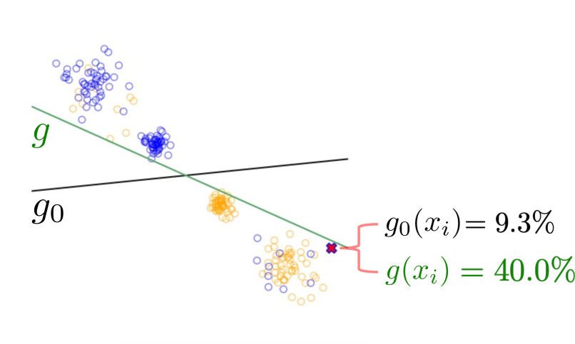
Figure 1: Classification models that make the same yes-or-no predictions can still assign conflicting risk predictions. Here, we show a 2D classification task with $n^{+{}}{}=200$ positive examples (blue) and $n^{-{}}{}=200$ negative examples (orange). We plot the decision boundary of a baseline model $g{}_{0}$ (black; log-loss/AUC/calibration = 0.41/0.88/17%) and a competing model that performs almost equally well $g(\bm{x}_{i})$ (green; log-loss/AUC/calibration = 0.42/0.89/16%). As shown, both classifiers make the same yes-or-no predictions, but assign conflicting risk estimates to individual examples e.g., example $\bm{x}_{i}$ is assigned a risk estimate of $g{}_{0}(\bm{x}_{i})=9.3\%$ by the baseline model but $g(\bm{x}_{i})=40.0\%$ by the competing model.

One way we compute predictive multiplicity is by constructing a range of individual risk predictions as a way to quantify pointwise uncertainty resulting from an underspecified empirical risk minimization problem. This relates to methods for evaluating predictive uncertainty such as conformal prediction (Shafer and Vovk 2008; Romano et al. 2020) as well as Bayesian approaches (see e.g., Dusenberry et al. 2020; Lum, Dunson, and Johndrow 2022). However, conformal prediction focuses on uncertainty that arises due to non-conformity between historical data and new data, which is orthogonal to our goal. We focus on a non-Bayesian approach, recognizing that non-Bayesian methods are very typical in applied machine learning. Our goals relate also to a line of work that aims to quantify and communicate uncertainty in machine learning (Hofman, Goldstein, and Hullman 2020; Kale, Kay, and Hullman 2020; McGrath et al. 2020; Soyer and Hogarth 2012; Kompa, Snoek, and Beam 2021b; Wei et al. 2022) and calibrate trust among stakeholders (Joslyn and LeClerc 2013). Other complementary work seeks interventions to resolve multiplicity (Ali, Lahoti, and Gummadi 2021) or ensembling (Black, Leino, and Fredrikson 2022).

2 Framework

We consider a probabilistic classification task with a dataset of $n$ examples $\mathcal{D}{}=\{(\bm{x}_{i},y_{i})\}_{i=1}^{n}$. Each example consists of a feature vector $\bm{x}_{i}=[1,x_{i1},\ldots,x_{id}]\in\mathcal{X}\subseteq\mathbb{R}^{d+1}$ and a label $y_{i}\in\mathcal{Y}=\{-1,+1\}$, where $y_{i}=+1$ is an event of interest (e.g., default on a loan). With the dataset, we train a probabilistic classifier $g{}:\mathcal{X}\to[0,1]$ – i.e., a model that assigns a risk estimate to example $\bm{x}_{i}$ as: $g{}(\bm{x}_{i}):=\text{Pr}(y_{i}=+1|\bm{x}_{i})$. We refer to this model as the baseline model, $g{}_{0}{}$, because it is the optimal solution to an empirical risk minimization (ERM) problem of the form:

$$\min_{g{}\in\mathcal{H}}L(g{};\mathcal{D}{}),$$ (1)

where $\mathcal{H}$ is a family of probabilistic classifiers, and $L(~{}\cdot~{};\mathcal{D}{})$ is a loss function evaluated on the dataset $\mathcal{D}{}$. In what follows, we write $L(g{})$ instead of $L(g{};\mathcal{D}{})$ for conciseness. We evaluate the performance of a model in terms of $L(g{})$, as well as the following metrics:

1. Risk Calibration: A risk-calibrated model assigns risk predictions that match observed frequencies (Naeini, Cooper, and Hauskrecht 2015). We measure risk calibration in terms of expected calibration error:

   $$\textrm{ECE}(g{})=\sum_{b=1}^{B}\frac{n_{b}}{n}|\hat{p}_{b}(g{})-\bar{p}_{b}|.$$ (2)

   Here: $I_{b}$ is the index set of $n_{b}$ examples in bin $b\in[B]$; and $\hat{p}_{b}(g{}):=\tfrac{1}{n_{b}}\sum_{i\in I_{b}}~{}g{}(\bm{x}_{i})$ and $\bar{p}_{b}=\tfrac{1}{n_{b}}\sum_{i\in I_{b}}\mathds{1}[y_{i}=+1]$ are the mean predicted risk and mean observed risk of examples in bin $b\in[B]$, respectively.

2. Rank Accuracy: A rank-accurate model outputs risk predictions that can be used to correctly order examples in terms of true risk. We assess rank accuracy using the area under the ROC curve:

   $$\textrm{AUC}(g{})=\frac{1}{n^{+{}}n^{-{}}}\sum_{\begin{subarray}{c}i:y_{i}=+1\\ k:y_{k}=-1\end{subarray}}\mathds{1}[g{}(\bm{x}_{i})>g{}(\bm{x}_{k})],$$ (3)

   where $n^{+{}}{}=|\{i:y_{i}=+1\}|$ and $n^{-{}}{}=|\{i:y_{i}=-1\}|$.

In what follows, we let $M(g{};\mathcal{D})\in\mathbb{R}_{+}$ denote the performance of $g{}\in\mathcal{H}$ over a dataset $\mathcal{D}$ in regards to performance metric $M(g)$, where the convention is that lower values of $M(g)$ are better; when working with AUC, we measure the AUC error: $M(g)=1-\textrm{AUC}(g)$.

2.1 Competing Models

Competing models are classifiers with near-optimal performance compared to the baseline model. A competing model is any model $g\in\mathcal{H}$ whose performance is within $\epsilon$ of the baseline model $g{}_{0}{}$.

Definition 1 ($\epsilon$-Level Set)

Given a baseline model $g{}_{0}{}$, metric $M$, and error tolerance $\epsilon>0$, the set of competing models ($\epsilon$-level set) is the set:

$$\!\mathcal{H}{}_{\epsilon}({g{}_{0}{}})\!:=\!\{g{}\in\mathcal{H}:M(g{})\leq M(g{}_{0}{})+\epsilon\}.$$

Our methods consider multiplicity over a range of $\epsilon$ values. In practice, a suitable choice of $\epsilon$ should reflect the epistemic uncertainty in the performance of the baseline model. For instance, one could employ bootstrap re-sampling to measure the model uncertainty due to sample variation or consider worst-case uncertainty through generalization bounds.

2.2 Measuring Viable Risk Predictions

To examine how multiplicity affects predictions, we define a range of viable risk estimates that can be assigned by competing models.

Definition 2 (Viable Prediction Range)

The viable prediction range is the smallest and largest risk estimate assigned to example $i$ over competing models in the $\epsilon$-level set:

$$V_{{\epsilon}}({\bm{x}_{i}}):=[\min_{g{}\in\mathcal{H}{}_{\epsilon}({g{}_{0}{}})}g{}(\bm{x}_{i}),\max_{g{}\in\mathcal{H}{}_{\epsilon}({g{}_{0}{}})}g{}(\bm{x}_{i})].$$ (4)

For a prediction task, computing the viable prediction ranges over a sample illuminates the extent to which competing models assign different risk estimates to individuals. Although we express the prediction range over an $\epsilon$-level set using $[\cdot,\cdot]$ interval notation, not all predictions between the min and the max may be attainable by a competing model.

2.3 Measuring Predictive Multiplicity

We say that a risk estimate is conflicting if it differs from the baseline risk estimate by at least some deviation threshold, $\delta\in(0,1)$. The appropriate value of $\delta$ will depend on the application; i.e. a conflicting risk prediction in a clinical decision support task may differ from that which constitutes a conflicting risk prediction in recidivism prediction.

Ambiguity and discrepancy reflect the proportion of examples in a sample $S$ assigned conflicting risk estimates by competing models. These definitions follow Marx, Du Pin Calmon, and Ustun (2020), who give analogous definitions for the problem of multiplicity with binary predictions (see Figure 1 for an illustration of the difference between this problem and the multiplicity of risk estimates).

Definition 3 (Ambiguity)

The $(\epsilon,\delta)$-ambiguity of a probabilistic classification task over a sample $S$ is the proportion of examples in $S$ whose baseline risk estimate changes by at least $\delta$ over the $\epsilon$-level set:

$$A_{{\delta},{\epsilon}}({g{}_{0}{}};{S}) :=\frac{1}{|S|}\sum_{i\in S}\mathds{1}[\max_{g{}\in\mathcal{H}{}_{\epsilon}({g{}_{0}{}})}|g{(\bm{x}_{i})}-g{}_{0}{}(\bm{x}_{i})|\geq\delta].$$

Relative to the baseline model, ambiguity makes a statement about the proportion of individuals whose risk estimate is uncertain by at least $\delta$. High ambiguity means more uncertainty in risk predictions. Users may also consult the viable prediction range to guide decisions using the baseline model.

Definition 4 (Discrepancy)

The $(\epsilon,\delta)$-discrepancy of a probabilistic classification task over a sample $S$ is the maximum proportion of examples in $S$ whose risk estimates could change by at least $\delta$ by switching the baseline model with a competing model in the $\epsilon$-level set:

$$D_{{\delta},{\epsilon}}({g{}_{0}{}};{S}):=\max_{g{}\in\mathcal{H}{}_{\epsilon}({g{}_{0}{}})}\frac{1}{|S|}\sum_{i\in S}\mathds{1}[|g{}(\bm{x}_{i})-g{}_{0}{}(\bm{x}_{i})|\geq\delta].$$

Relative to the baseline model, discrepancy reflects the maximum the number of conflicting risk estimates as a result of replacing baseline model with a competing model in the $\epsilon$-level set.

Ambiguity and discrepancy differ in the stance they take in regard to the worst case. Discrepancy measures the worst-case number of predictions that will change by switching the baseline model with a competing model. In contrast, ambiguity focuses on the worst case for prediction variation over the set of competing models. If we were to abstain from prediction on points that are assigned a conflicting prediction by a competing model (using e.g., selective classification methods Black, Leino, and Fredrikson 2022), then ambiguity would reflect the abstention rate.

Computing Ambiguity with Viable Prediction Ranges.

As shown in Figure 2, we can use the viable prediction ranges of all points in a sample to compute ambiguity. Given the viable prediction range for each example, we can calculate the maximum difference between the baseline risk and that assigned by competing models. We can then compute ambiguity by measuring the proportion of examples where this difference exceeds the deviation threshold.

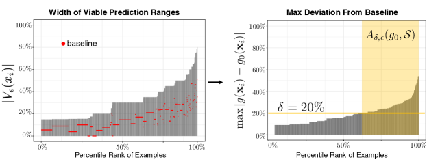
Figure 2: An illustration of how viable prediction ranges relate to ambiguity. Left, we plot the width of the viable prediction ranges $\left|V_{{\epsilon}}({\bm{x}_{i}})\right|$ on the $y$-axis for each example on the $x$-axis. Note that widths shifted to start from zero and examples shown in increasing order. The plot also shows the individual baseline risk estimates for each example in red $g{}_{0}{(\bm{x}_{i})}- \min_{g\in\mathcal{H}_{\epsilon}(g{}_{0})}g{}(\bm{x}_{i})$ (shifted similarly). To interpret, the first example from the left has a width of $\approx 15\%$ with a baseline risk estimate on the lower side of the range. The last example has a width of $\approx 80\%$ with a baseline risk estimate closer to the higher side of the range. Using the viable prediction ranges $V_{{\epsilon}}({\bm{x}_{i}})$ directly, we can extract the maximum difference from the baseline. On the right, we plot the maximum deviation from the baseline, $\max\left|g{}(\bm{x}_{i})-g{}_{0}{}(\bm{x}_{i})\right|$ for each example on the $x$-axis (increasing order). To interpret, consider a deviation threshold $\delta=20\%$, all examples with max deviation above that threshold are highlighted in yellow giving us ambiguity, $A_{{\delta},{\epsilon}}({g{}_{0}{}};{S})$.

3 Methodology

In this section, we detail the procedure for computing measures of predictive multiplicity. This methodology can be applied to any convex loss function $L(\cdot)$, and together with a training problem that employs a convex regularization term. We illustrate the methodology on the classification task described in §2 by training a probabilistic classifier via logistic regression, with $g{}(\bm{x}_{i})=\frac{1}{1+\exp(-\langle\bm{w},\bm{x}_{i}\rangle)}$ , where $\bm{w}=[w_{0},w_{1},\ldots,w_{d}]^{\top}\in\mathbb{R}^{d+1}$ is a coefficient vector. We train this baseline model by solving Eq. (1) to minimize normalized logistic loss: $L(\bm{w})=\tfrac{1}{n}\sum_{i=1}^{n}\log(1+\exp(-\langle{\bm{w}},{y_{i}\bm{x}_{i}}\rangle))$.

3.1 Measuring Ambiguity

We first present a method for computing ambiguity for different choices of $\epsilon$ and $\delta$. The method also gives a conservative approximation of the viable prediction range for each example. We construct a pool of candidate models that assign a specific risk estimate to each example. From these models, we select those with performance within $\epsilon$ of the baseline model as the set of competing models.

Definition 5 (Candidate Model)

Given a baseline model $g{}_{0}{}$, a finite set of user-specified threshold probabilities $P\subseteq[0,1]$, then for each $p\in P$ a candidate model for example $\bm{x}_{i}$ is an optimal solution to the following constrained ERM:

$$\begin{split}\min_{\bm{w}\in\mathbb{R}^{d+1}}&\ L(\bm{w})\\ \textnormal{s.t.}\quad&g{}(\bm{x}_{i})\leq p,\;\;\textrm{if}~{}p<g{}_{0}{}(\bm{x}_{i})\\ &g{}(\bm{x}_{i})\geq p.\;\;\;\textrm{if}~{}p>g{}_{0}{}(\bm{x}_{i})\end{split}$$ (5)

For each threshold probability $p\in P$, we train a candidate model $g{}$ such that the probability assigned to the example is constrained to the threshold $p$. In this way, by training for each example and threshold probability $p\in P$, we obtain the set of candidate models $\mathcal{G}:=\{g{}:i\in S,p\in P\}$. We choose to solve the instances in order of increasing values of threshold probability $p$, which allows us to warm-start the optimization using previous solutions.

Given the set of candidate models, we define a candidate $\epsilon$-level set as

$$\tilde{\mathcal{H}}_{\epsilon}(g{}_{0}{}) \!=\!\{g\in\mathcal{G}:M(g{})\!\leq\!M(g_{0})\!+\!\epsilon\}.$$ (6)

We use the candidate $\epsilon$-level set to compute measures of predictive multiplicity. This method is exact for ambiguity defined in terms of near-optimal loss when the grid of threshold probabilities $P\subseteq[0,1]$ aligns with $g{}_{0}{(x_{i})}\pm\delta$ (i.e., is selected as appropriate to the baseline prediction for an example and the value of $\delta$). For other metrics, such as AUC, this approach to compute ambiguity gives a conservative estimate (i.e., lower bound)—the training of a candidate model does not directly optimize for AUC, but we can retain only those candidate models that are competitive for the appropriate $\epsilon$-level set definition. Since $\tilde{\mathcal{H}}_{\epsilon}(g{}_{0}{})\subseteq\mathcal{H}{}_{\epsilon}({g{}_{0}{}})$, the candidate-model approach also provides a conservative estimate of the viable prediction range (Eq. (4)) for an example.

3.2 Measuring Discrepancy

Discrepancy is the maximum proportion of examples assigned conflicting risk estimates by a single competing model, $g{}\in\mathcal{H}{}_{\epsilon}({g{}_{0}{}})$. Recall that a conflicting risk estimate differs from the baseline risk estimate $g{}_{0}{(\bm{x}_{i})}$ by at least some deviation threshold, $\delta>0$. Therefore, measuring discrepancy with respect to a baseline model corresponds to solving the following maximization problem:

$$\begin{split}\max_{g{}\in\mathcal{H}{}_{\epsilon}({g{}_{0}{}})}&\qquad\sum_{i\in S}\mathds{1}[|g{}(\bm{x}_{i})-g{}_{0}{(\bm{x}_{i})}|\geq\delta].\end{split}$$ (7)

Given a sample $S$, the baseline loss $L_{0}$, error tolerance $\epsilon$, and deviation threshold $\delta$, we can formulate Eq. (7) as a mixed-integer non-linear program (MINLP):

@c@r@ c@ l¿ l¿ r@  max_w∈R^d+1 &  ∑_i∈S d_i
s.t. L(w) ≤ L_0 + ϵ
d_i = v_i, δ+ z_i, δ ∀i∈S    
M_z,i(1 - z_i, δ) ≥ ⟨w,x_i ⟩ - U_i, δ ∀i∈S
M_v, i(1 - v_i, δ) ≥-⟨w,x_i ⟩ + B_i, δ ∀i∈S
d_i, z_i, δ, v_i, δ ∈ {0,1} ∀i∈S

The MINLP in (8) fits the parameters of a linear classifier that maximizes discrepancy . Here, the objective maximizes number of examples assigned a conflicting risk estimate using the indicator variables $d_{i}:=\mathds{1}[|g{}(\bm{x}_{i})-g{}_{0}{(\bm{x}_{i})}|\geq\delta]$. Each $d_{i}$ is set to $z_{i,\delta}:=\mathds{1}[g{}(\bm{x}_{i})\leq({g{}_{0}(\bm{x}_{i})-\delta})]$ (or $v_{i,\delta}:=\mathds{1}[g{}(\bm{x}_{i})\geq({g{}_{0}(\bm{x}_{i})+\delta})]$) when the model assigns a risk estimate to example $i$ that exceeds $\delta$ on the low-side (or high-side) of the baseline risk estimate, respectively. We ensure the indicator behavior of $z_{i,\delta}$ and $v_{i,\delta}$ through the “Big-M” constraints (8) and (8), which flag deviations in score space. The Big-M parameters can be set as $M_{z,i}:=-U_{i,\delta}+\max_{\bm{w}}\langle{\bm{w}},{\bm{x}_{i}}\rangle$ and $M_{v,i}:=B_{i,\delta}-\min_{\bm{w}}\langle{\bm{w}},{\bm{x}_{i}}\rangle$, where $U_{i,\delta}:=\textrm{logit}({g{}_{0}(\bm{x}_{i})-\delta})$, and $B_{i,\delta}:=\textrm{logit}({g{}_{0}(\bm{x}_{i})+\delta})$. When the values of $U_{i,\delta}$ and $B_{i,\delta}$ lie outside of the $[0,1]$ domain of the logit, we can drop the relevant indicator variable from the formulation. We provide additional details in the Appendix.

Outer-Approximation Algorithm.

The challenge in solving (8) is that constraint (8) is non-linear. We construct a linear approximation of the loss (see e.g., Franc and Sonnenburg 2008; Joachims, Finley, and Yu 2009) using an iterative, outer-approximation method (see e.g., Ustun and Rudin 2017; Bertsimas et al. 2016; Bertsimas and King 2017) to solve. The algorithm recovers a globally optimal solution to the MINLP in (8), and can be implemented using a mixed-integer programming solver with callback functions (see e.g., Ustun and Rudin 2017; Bertsimas et al. 2016; Bertsimas and King 2017). The procedure builds a branch-and-bound tree to discover integer-feasible solutions that obey all constraints other than (8). For each feasible solution identified, the procedure computes its loss to determine if it is feasible with respect to constraint (8). If feasible, the procedure retains the solution. Otherwise, it updates the loss function approximation by adding a new linear constraint.

This method is exact for computing discrepancy in terms of near-optimal loss. For other metrics, we can again treat the intermediate solutions to the outer-approximation algorithm as candidate models and use these candidates to recover a lower bound similar to the method used in § 3.1.

4 Numerical Experiments

In this section, we present experiments on synthetic and real-world data. Our goals are to: (1) reveal dataset characteristics that impact predictive multiplicity; and (2) determine the extent to which real risk assessment tasks exhibit predictive multiplicity in practice.

4.1 Synthetic Datasets

Linear Separability.

To demonstrate how separability informs predictive multiplicity, we compute ambiguity while varying the degree of separability and show results in Figure 3 column (A). We set $\delta=20\%$ and $\epsilon=5\%$ and control separability by increasing the variance of the data from $\sigma=4$ (top) to $\sigma=10$ (bottom). A clear trend is that ambiguity increases as the data becomes less separable from $1\%$ to $21\%$. Notice, also that the ambiguous examples tend to be those near the discriminant boundary and outliers.

Outliers and Margin Distance.

We examine how predictive multiplicity relates to outlier distance from the discriminant boundary. We position outliers near and far from the discriminant boundary and compute ambiguity. As shown in Figure 3 column (B), a clear trend is that examples that are outliers but far from the discriminant boundary (high margin) are less susceptible to predictive multiplicity.

Majority-Minority Structure.

We consider the effect of systematically varying the majority-minority structure of data. For this, we generate a majority class that has a different statistical pattern of features than a minority class. Given the two groups, the model is faced with a tradeoff between correctly predicting one group or the other. In Figure 3 column (C), we vary the ratio in a majority-minority structure revealing that the minority group is more prone to predictive multiplicity. The ambiguity of the minority group at 10:1 is substantially larger than for the majority group. This shows the importance of evaluating multiplicity across subgroups.

More Separable, $A_{{\delta},{\epsilon}}({g{}_{0}{}};{S})=1\%$	Large Margin, $A_{{\delta},{\epsilon}}({g{}_{0}{}};{S})=1\%$	Ratio 10:1, $A_{{\delta},{\epsilon}}({g{}_{0}{}};{S})=7\%$
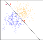
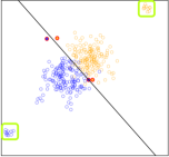
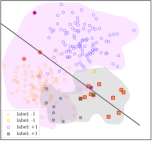
Less Separable, $A_{{\delta},{\epsilon}}({g{}_{0}{}};{S})=21\%$	Small Margin, $A_{{\delta},{\epsilon}}({g{}_{0}{}};{S})=3\%$	Ratio 1:1, $A_{{\delta},{\epsilon}}({g{}_{0}{}};{S})=53\%$

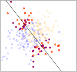
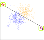
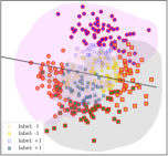
Figure 3: Experiments on synthetic data. In (A), we vary separability and find that ambiguity increases as separability decreases. In (B), we position outliers near and away from the discriminant boundary finding that outliers closer to the boundary are more prone to ambiguity. In (C), we vary the ratio in a majority-minority structured dataset: magenta shading- majority group (circles), grey shading- minority group (squares) revealing that the minority group is more prone to ambiguity. In the figures, $Y=+1$ examples are blue, $Y=-1$ examples are orange, and ambiguous examples are highlighted red and we set $\delta=20\%$ and $\epsilon=5\%$.

	mammo: breast cancer	apnea: sleep apnea	arrest: crime rearrest

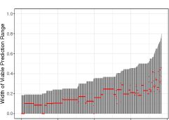
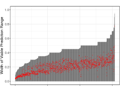
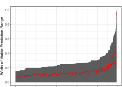
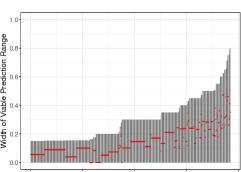
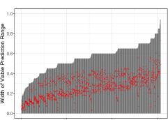
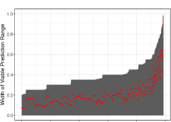
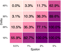
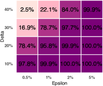
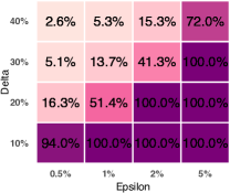
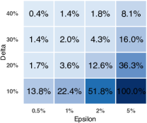
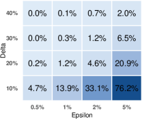
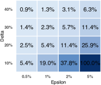
Figure 4: Predictive multiplicity in probabilistic classification on mammo, apnea and arrest. In rows (A) and (B) we show the distribution of viable prediction ranges $|V_{\epsilon}(\bm{x}_{i})|$ on the y-axis for each example on the x-axis (relative baseline estimates in red). Notice, pointwise viable prediction ranges are plotted in increasing order from left to right. We plot viable prediction ranges for competing models with near-optimal training AUC (A) and training loss (B). See illustration in Figure 2. We also show ambiguity (C) and discrepancy (D) for competing models with respect to training loss. We include other datasets in Appendix E.

4.2 Real-World Datasets

In this section, we evaluate predictive multiplicity in risk prediction tasks from medicine, lending, and criminal justice. Altogether, we consider seven datasets that exhibit variations in sample size, number of features, and class imbalance (see Table 1 in the Appendix). For each dataset, we compute viable prediction ranges, ambiguity and discrepancy using the methods outlined in §3. When training candidate models, we adopt a grid of target predictions: $P=\{0.01,0.1,0.2,\ldots,0.9,0.99\}$. We compute discrepancy by solving the MINLP Eq. (7) with CPLEX v20.1 (Diamond and Boyd 2016) on a single CPU with 16GB RAM. Our results are shown in Figure 4, and additional results are in the Appendix.

Viable Prediction Ranges.

Our results show that competing models can assign risk estimates that vary substantially. Viable prediction ranges are plotted in rows (A) and (B) of Figure 4, and we see non-zero viable prediction ranges for all examples across all datasets. The viable ranges for apnea and mammo appear much larger compared to compas_arrest. In terms of near-optimal loss, apnea has the most variation, while mammo has the most variation in terms of AUC. This points to the value in varying near-optimal metric.

Ambiguity and Discrepancy.

Ambiguity and discrepancy are shown in rows (C) and (D) of Figure 4, respectively. For $\epsilon=1\%$ and $\delta=20\%$, we see ambiguity values at $35.3\%$ (mammo), $95.8\%$ (apnea), and $51.4\%$ (compas_arrest). This means that $35.3\%$ of breast cancer risk estimates vary by at least $20\%$ over near-optimal models. We see discrepancy values at $3.6\%$ (mammo), $1.2\%$ (apnea), and $5.4\%$ (compas_arrest) for $\epsilon=1\%$ and $\delta=20\%$. compas_arrest is the worst in terms of discrepancy, while apnea has the most severe ambiguity. Thus, ambiguity and discrepancy are not always coupled.

On the Choice of Performance Metric.

In settings where we want a model that performs well in terms of AUC, we should measure predictive multiplicity over a set of competing models with near-optimal AUC. In practice, it is often convenient to measure predictive multiplicity over a set of competing models that attain near-optimal loss (since the loss can be encoded into an optimization problem). This is a problem because small variations in loss can lead to large variations in AUC – thus models with near-optimal loss may not match models with near-optimal AUC. Our results show that measures of predictive multiplicity vary considerably based on the performance metric used to define the set of competing models. In particular, we find that discrepancy and ambiguity will vary when measured over competing models that attain near-optimal loss, AUC, or ECE.

On Samples Prone to Ambiguity.

Our results reveal a relationship between ambiguity and individual uniqueness (number of duplicates), class imbalance, and baseline risk estimate. For uniqueness, we find that across datasets, less than $10\%$ of examples with more than $20$ duplicates are ambiguous. That unique examples are more prone to ambiguity is related to our findings on outliers (see §4.1).

In terms of class imbalance, we find datasets with class imbalance skewed negative (adult, bank) often exhibit multiplicity on positive examples. In comparison, datasets that are roughly balanced by class (e.g., mammo, compas_arrest) have the same level of ambiguity for each class. This can be interpreted in light of the majority-minority effect from §4.1.

In terms of the baseline risk estimate, we see high ambiguity for examples with baseline risk near 50% on all datasets. For instance, all examples with baseline risk between $45\%$ and $55\%$ are ambiguous for the mammo dataset ($\epsilon=0.5\%$ AUC, $\delta=20\%$). There is no reason to believe that high ambiguity is less problematic for these samples. Rather, the importance of ambiguity will depend on the risk thresholds that drive decisions in a particular domain.

On the Disparate Impact of Multiplicity.

Our results demonstrate how multiplicity can disproportionately impact individuals from historically marginalized groups. For example, when predicting the risk of rearrest, individuals who are ethnically Hispanic are disproportionately affected by predictive multiplicity: ambiguity is $39\%$ for African Americans and $49\%$ for Caucasians, compared to $98\%$ for Hispanics ($\epsilon=1\%$ and $\delta=20\%$). Hence, reporting predictive multiplicity for subgroups can reveal important fairness considerations when testing models deployed throughout society.

5 Concluding Remarks

We developed methods to evaluate the effect of slightly perturbing optimal model performance, revealing that similar models do not always assign similar predictions. We studied how competing models can assign conflicting predictions in probabilistic classification tasks. The proposed optimization-based methods compute our simple measures reliably. Compared to previous work, our methods allow for flexibility in choosing near-optimal metric and deviation threshold. Using synthetic data, we also present the first study providing insight into the kinds of data characteristics that give rise to predictive multiplicity and show that separability, outliers and majority-minority structure are informative. Empirically, we reveal concerning levels of predictive multiplicity in high-stakes domains.

More research is needed to examine predictive multiplicity for other loss functions and model classes (our methods immediately generalize to linear models with convex loss functions). Also, it will be important to study how to effectively communicate these effects to practitioners and decision makers. Also, when a practitioner encounters high predictive multiplicity, more work is needed on response options and mitigation strategies. Given predictive multiplicity metrics, practitioners can make better decisions in model selection while end-users can adjust their reliance on individual risk predictions. Concisely, analyzing predictive multiplicity promotes accountability and transparency in machine learning.

References

- Ali, Lahoti, and Gummadi (2021) Ali, J.; Lahoti, P.; and Gummadi, K. P. 2021. Accounting for Model Uncertainty in Algorithmic Discrimination, volume 1. Association for Computing Machinery. ISBN 9781450384735.
- Attigeri, Pai, and Pai (2017) Attigeri, G. V.; Pai, M. M.; and Pai, R. M. 2017. Credit risk assessment using machine learning algorithms. Advanced Science Letters, 23(4): 3649–3653.
- Austin, Ocker, and Bhati (2010) Austin, J.; Ocker, R.; and Bhati, A. 2010. Kentucky Pretrial Risk Assessment Instrument Validation. The JFA Institute, 5.
- Bekhet and Eletter (2014) Bekhet, H. A.; and Eletter, S. F. K. 2014. Credit risk assessment model for Jordanian commercial banks: Neural scoring approach. Review of Development Finance, 4(1): 20–28.
- Bertsimas and King (2017) Bertsimas, D.; and King, A. 2017. Logistic regression: From art to science. Statistical Science, 367–384.
- Bertsimas et al. (2016) Bertsimas, D.; King, A.; Mazumder, R.; et al. 2016. Best subset selection via a modern optimization lens. Annals of statistics, 44(2): 813–852.
- Black and Fredrikson (2021) Black, E.; and Fredrikson, M. 2021. Leave-One-out Unfairness. In Proceedings of the 2021 ACM Conference on Fairness, Accountability, and Transparency, FAccT ’21, 285–295. New York, NY, USA: Association for Computing Machinery. ISBN 9781450383097.
- Black, Leino, and Fredrikson (2022) Black, E.; Leino, K.; and Fredrikson, M. 2022. Selective Ensembles for Consistent Predictions. In International Conference on Learning Representations.
- Black, Raghavan, and Barocas (2022) Black, E.; Raghavan, M.; and Barocas, S. 2022. Model Multiplicity: Opportunities, Concerns, and Solutions. In 2022 ACM Conference on Fairness, Accountability, and Transparency, FAccT ’22, 850–863. New York, NY, USA: Association for Computing Machinery. ISBN 9781450393522.
- Breiman (2001) Breiman, L. 2001. Statistical modeling: The two cultures. Statistical Science, 16(3): 199–215.
- Chatfield (1995) Chatfield, C. 1995. Model Uncertainty, Data Mining and Statistical Inference. Journal of the Royal Statistical Society. Series A (Statistics in Society), 158(3): 419.
- Chen et al. (2021) Chen, I. Y.; Joshi, S.; Ghassemi, M.; and Ranganath, R. 2021. Probabilistic machine learning for healthcare. Annual Review of Biomedical Data Science, 4: 393–415.
- Christin, Rosenblat, and Boyd (2015) Christin, A.; Rosenblat, A.; and Boyd, D. 2015. Courts and predictive algorithms. Data & civil rights: A new era of policing and justice, 13.
- Coston, Rambachan, and Chouldechova (2021) Coston, A.; Rambachan, A.; and Chouldechova, A. 2021. Characterizing Fairness Over the Set of Good Models Under Selective Labels. CoRR, abs/2101.00352.
- D’Amour et al. (2022) D’Amour, A.; Heller, K.; Moldovan, D.; Adlam, B.; Alipanahi, B.; Beutel, A.; Chen, C.; Deaton, J.; Eisenstein, J.; Hoffman, M. D.; Hormozdiari, F.; Houlsby, N.; Hou, S.; Jerfel, G.; Karthikesalingam, A.; Lucic, M.; Ma, Y.; McLean, C.; Mincu, D.; Mitani, A.; Montanari, A.; Nado, Z.; Natarajan, V.; Nielson, C.; Osborne, T. F.; Raman, R.; Ramasamy, K.; Sayres, R.; Schrouff, J.; Seneviratne, M.; Sequeira, S.; Suresh, H.; Veitch, V.; Vladymyrov, M.; Wang, X.; Webster, K.; Yadlowsky, S.; Yun, T.; Zhai, X.; and Sculley, D. 2022. Underspecification Presents Challenges for Credibility in Modern Machine Learning. Journal of Machine Learning Research, 23(226): 1–61.
- Diamond and Boyd (2016) Diamond, S.; and Boyd, S. 2016. CVXPY: A Python-embedded modeling language for convex optimization. Journal of Machine Learning Research, 17: 1–5.
- Dong and Rudin (2020) Dong, J.; and Rudin, C. 2020. Exploring the cloud of variable importance for the set of all good models. Nature Machine Intelligence, 2(12): 810–824.
- Dusenberry et al. (2020) Dusenberry, M. W.; Tran, D.; Choi, E.; Kemp, J.; Nixon, J.; Jerfel, G.; Heller, K.; and Dai, A. M. 2020. Analyzing the role of model uncertainty for electronic health records. ACM CHIL 2020 - Proceedings of the 2020 ACM Conference on Health, Inference, and Learning, 204–213.
- Fisher, Rudin, and Dominici (2019) Fisher, A.; Rudin, C.; and Dominici, F. 2019. All models are wrong, but many are useful: Learning a variable’s importance by studying an entire class of prediction models simultaneously. Journal of Machine Learning Research, 20(Vi).
- Franc and Sonnenburg (2008) Franc, V.; and Sonnenburg, S. 2008. Optimized cutting plane algorithm for support vector machines. In Proceedings of the 25th International Conference on Machine Learning, 320–327. ACM.
- Hamid et al. (2017) Hamid, K.; Asif, A.; Abbasi, W.; Sabih, D.; et al. 2017. Machine learning with abstention for automated liver disease diagnosis. In 2017 International Conference on Frontiers of Information Technology (FIT), 356–361. IEEE.
- Hofman, Goldstein, and Hullman (2020) Hofman, J. M.; Goldstein, D. G.; and Hullman, J. 2020. How Visualizing Inferential Uncertainty Can Mislead Readers about Treatment Effects in Scientific Results. Conference on Human Factors in Computing Systems - Proceedings.
- Joachims, Finley, and Yu (2009) Joachims, T.; Finley, T.; and Yu, C.-N. J. 2009. Cutting-plane training of structural SVMs. Machine Learning, 77(1): 27–59.
- Joslyn and LeClerc (2013) Joslyn, S.; and LeClerc, J. 2013. Decisions With Uncertainty: The Glass Half Full. Current Directions in Psychological Science, 22(4): 308–315.
- Kale, Kay, and Hullman (2020) Kale, A.; Kay, M.; and Hullman, J. 2020. Visual Reasoning Strategies for Effect Size Judgments and Decisions. IEEE Transactions on Visualization and Computer Graphics, 1–1.
- Khand et al. (2017) Khand, A.; Frost, F.; Grainger, R.; Fisher, M.; Chew, P.; Mullen, L.; Patel, B.; Obeidat, M.; Albouaini, K.; Dodd, J.; Goldstein, S. A.; Newby, L. K.; Cyr, D. D.; Neely, M.; Lüscher, T. F.; Brown, E. B.; White, H. D.; Ohman, E. M.; Roe, M. T.; Hamm, C. W.; Six, A. J.; Backus, B. E.; and Kelder, J. C. 2017. Heart Score Value. Netherlands Heart Journal, 10(6): 1–10.
- Kompa, Snoek, and Beam (2021a) Kompa, B.; Snoek, J.; and Beam, A. L. 2021a. Second opinion needed: communicating uncertainty in medical machine learning. NPJ Digital Medicine, 4(1): 1–6.
- Kompa, Snoek, and Beam (2021b) Kompa, B.; Snoek, J.; and Beam, A. L. 2021b. Second opinion needed: communicating uncertainty in medical machine learning. npj Digital Medicine, 4(1).
- Latessa et al. (2010) Latessa, E. J.; Lemke, R.; Makarios, M.; Smith, P.; and Lowenkamp, C. T. 2010. The creation and validation of the ohio risk assessment system (ORAS). Federal Probation, 74(1): 16–22.
- Lum, Dunson, and Johndrow (2022) Lum, K.; Dunson, D. B.; and Johndrow, J. 2022. Closer than they Appear: A Bayesian Perspective on Individual-Level Heterogeneity in Risk Assessment. Journal of the Royal Statistical Society Series A: Statistics in Society, 185(2): 588–614.
- Marx, Du Pin Calmon, and Ustun (2020) Marx, C. T.; Du Pin Calmon, F.; and Ustun, B. 2020. Predictive Multiplicity in Classification. In Proceedings of the 37th International Conference on Machine Learning, ICML’20. JMLR.org.
- McGrath et al. (2020) McGrath, S.; Mehta, P.; Zytek, A.; Lage, I.; and Lakkaraju, H. 2020. When Does Uncertainty Matter?: Understanding the Impact of Predictive Uncertainty in ML Assisted Decision Making. CoRR, abs/2011.06167.
- Moreno et al. (2005) Moreno, R. P.; Metnitz, P. G.; Almeida, E.; Jordan, B.; Bauer, P.; Campos, R. A.; Iapichino, G.; Edbrooke, D.; Capuzzo, M.; and Le Gall, J. R. 2005. SAPS 3 - From evaluation of the patient to evaluation of the intensive care unit. Part 2: Development of a prognostic model for hospital mortality at ICU admission. Intensive Care Medicine, 31(10): 1345–1355.
- Mozannar and Sontag (2020) Mozannar, H.; and Sontag, D. 2020. Consistent estimators for learning to defer to an expert. In International Conference on Machine Learning, 7076–7087. PMLR.
- Naeini, Cooper, and Hauskrecht (2015) Naeini, M. P.; Cooper, G. F.; and Hauskrecht, M. 2015. Binary classifier calibration using a Bayesian non-parametric approach. SIAM International Conference on Data Mining 2015, SDM 2015, 208–216.
- Pawelczyk, Broelemann, and Kasneci (2020) Pawelczyk, M.; Broelemann, K.; and Kasneci, G. 2020. On counterfactual explanations under predictive multiplicity. Proceedings of the 36th Conference on Uncertainty in Artificial Intelligence, UAI 2020, 124: 839–848.
- Romano et al. (2020) Romano, Y.; Barber, R. F.; Sabatti, C.; and Candès, E. 2020. With Malice Toward None: Assessing Uncertainty via Equalized Coverage. Harvard Data Science Review, 1–14.
- Semenova and Rudin (2019) Semenova, L.; and Rudin, C. 2019. A study in Rashomon curves and volumes: A new perspective on generalization and model simplicity in machine learning. CoRR, abs/1908.01755.
- Shafer and Vovk (2008) Shafer, G.; and Vovk, V. 2008. A tutorial on conformal prediction. Journal of Machine Learning Research, 9: 371–421.
- Soyer and Hogarth (2012) Soyer, E.; and Hogarth, R. M. 2012. The illusion of predictability: How regression statistics mislead experts. International Journal of Forecasting, 28(3): 695–711.
- Stokes et al. (2020) Stokes, J. M.; Yang, K.; Swanson, K.; Jin, W.; Cubillos-Ruiz, A.; Donghia, N. M.; MacNair, C. R.; French, S.; Carfrae, L. A.; Bloom-Ackermann, Z.; et al. 2020. A deep learning approach to antibiotic discovery. Cell, 180(4): 688–702.
- Than et al. (2014) Than, M.; Flaws, D.; Sanders, S.; Doust, J.; Glasziou, P.; Kline, J.; Aldous, S.; Troughton, R.; Reid, C.; Parsonage, W. A.; Frampton, C.; Greenslade, J. H.; Deely, J. M.; Hess, E.; Sadiq, A. B.; Singleton, R.; Shopland, R.; Vercoe, L.; Woolhouse-Williams, M.; Ardagh, M.; Bossuyt, P.; Bannister, L.; and Cullen, L. 2014. Development and validation of the emergency department assessment of chest pain score and 2h accelerated diagnostic protocol. EMA - Emergency Medicine Australasia, 26(1): 34–44.
- Ustun and Rudin (2017) Ustun, B.; and Rudin, C. 2017. Optimized Risk Scores. In Proceedings of the 23rd ACM SIGKDD International Conference on Knowledge Discovery and Data Mining. ACM.
- Veitch et al. (2021) Veitch, V.; D’Amour, A.; Yadlowsky, S.; and Eisenstein, J. 2021. Counterfactual invariance to spurious correlations: Why and how to pass stress tests. arXiv preprint arXiv:2106.00545.
- Wei et al. (2022) Wei, D.; Nair, R.; Dhurandhar, A.; Varshney, K. R.; Daly, E. M.; and Singh, M. 2022. On the Safety of Interpretable Machine Learning: A Maximum Deviation Approach. In Oh, A. H.; Agarwal, A.; Belgrave, D.; and Cho, K., eds., Advances in Neural Information Processing Systems.
- Zeng, Ustun, and Rudin (2017) Zeng, J.; Ustun, B.; and Rudin, C. 2017. Interpretable classification models for recidivism prediction. Journal of the Royal Statistical Society: Series A (Statistics in Society), 180(3): 689–722.