New-hires	Firm random
	RAIS	sample	sample
	(1)	(2)	(3)
Panel A. Worker characteristics
Average age	34.966	30.304	32.845
Male	0.580	0.635	0.619
White	0.606	0.574	0.600
Elementary school or less	0.376	0.410	0.408
Completed high school	0.471	0.532	0.510
Completed university	0.153	0.058	0.082

Panel B. Earnings     Mean monthly salary (Reals) 1288.915 807.502 1066.613 Median monthly salary (Reals) 742.429 621.422 686.848 Share of mean earnings divisible by 10 0.037 0.072 0.041 Share of mean earnings divisible by 100 0.017 0.034 0.018 Share of mean earnings divisible by 1,000 0.003 0.006 0.003 Share of contracted earnings divisible by 10 0.180 0.295 0.230 Share of contracted earnings divisible by 100 0.066 0.121 0.084 Share of contracted earnings divisible by 1,000 0.010 0.019 0.013

Panel C. Industry     Primary sector 0.046 0.034 0.026 Construction and utilities 0.140 0.167 0.195 Manufacturing 0.121 0.174 0.153 Retail 0.257 0.359 0.368 Services 0.437 0.265 0.259

Panel D. Region     North 0.054 0.050 0.048 Northeast 0.176 0.149 0.156 Southeast 0.506 0.521 0.530 South 0.173 0.187 0.189 Midwest 0.092 0.093 0.077

Number of observations 842,196,095 206,685,308 28,087,000

Notes: This table shows summary statistics on workers in the Relação Anual de Informações Sociais (RAIS), the new-hires sample, and the firm random sample. See Section LABEL:sec:context-data for sample definitions. Earnings are expressed in Brazilian Reals.

Notes: This table displays estimates of $\beta$ from equation (LABEL:reg:firm-outcomes). Each column shows the result of a regression using the dependent variable listed in the column header. In column 1, the outcome equals one if a new hire separated from the firm during the year she was hired (year $t$) or the following year (year $t+1$), and zero otherwise. Column 2 is defined analogously but using worker resignation likelihood instead of separation likelihood. In column 3, the dependent variable is the percent change in the number of workers employed between consecutive years. In column 4, the outcome is a dummy that equals one if the firm had no workers at the end of the year and zero otherwise.

I use the firm random sample to estimate all regressions. In columns 1 and 2, the regressions are estimated at the worker-by-firm-by-year level and only using data from the year in which a worker was hired and the following year. In columns 3 and 4, the regressions are estimated at the firm-by-year level.

The regressions control for firm age, share of employees with completed high school, share of employees with completed college, educational attainment of the firm manager, a dummy for having an HR department, the mean earnings of the firm employees, firm size fixed effects, number of hires fixed effects, and industry-by-microregion-by-year fixed effects. The specifications in columns 1 and 2 additionally control for worker gender, race, and occupation.

Heteroskedasticity-robust standard errors clustered at the firm level in parentheses. ^∗∗∗, ^∗∗ and ^∗ denote significance at the 1%, 5% and 10% levels.

& No Yes No Yes No Yes

Notes: This table displays estimates of $\beta$ from equation (LABEL:reg:firm-outcomes). In columns 1 and 2, the outcome is a dummy that equals one if the change in worker’s $i$’s contracted salary between $t$ and $t+1$‘, measured in Brazilian Reals, is a round number and zero otherwise. In columns 3 and 4, the outcome is a dummy that equals one if the percent change between $t$ and $t+1$ of worker $i$’s contracted salary is an integer and zero otherwise. In columns 5 and 6, the outcome equals one if either the absolute wage change is a round number or the percent change is an integer and zero otherwise.

I use the firm random sample to estimate all regressions. The regressions are estimated at the worker-by-firm-by-year level and only using data from the year in which a worker was hired and the following year. Even columns exclude new hires whose salary did not change in nominal terms.

The regressions control for worker gender, worker race, worker occupation, firm age, share of employees with completed high school, share of employees with completed college, educational attainment of the firm manager, a dummy for having an HR department, the mean earnings of the firm employees, firm size fixed effects, number of hires fixed effects, and industry-by-microregion-by-year fixed effects.

Heteroskedasticity-robust standard errors clustered at the firm level in parentheses. ^∗∗∗, ^∗∗ and ^∗ denote significance at the 1%, 5% and 10% levels.

&$-$0.972^∗∗∗$-$0.879^∗∗∗$-$0.012^∗∗∗$-$0.032^∗∗∗ (0.034)(0.086)(0.001)(0.001) Firm hiring experience (logs)$-$0.882^∗∗∗$-$0.053$-$0.025^∗∗∗$-$0.002^∗∗ (0.050)(0.140)(0.001)(0.001) Fixed firm sample? No Yes No Yes Notes: This table shows linear correlations between the covariate listed in the row header and the outcome listed in the column header.

In columns 1–2, the dependent variable is the estimated fraction of workers hired through coarse wage-setting, $\hat{\theta}$. Section LABEL:sub:bunching describes how $\hat{\theta}$ is estimated. Each observation denotes the excess mass at each value taken by a covariate. Thus, the sample size varies by covariate. For log CPI, $N=1,980$. For firm size and hiring experience, $N=100$.

In columns 3–4, the dependent variable is a dummy that equals one for workers hired at a round-numbered salary ($\mathbbm{1}\{w_{i}\in R\}$). In addition to the variables listed in the table, the regressions control for worker gender, worker race, worker occupation, worker education, worker potential experience, firm fixed effects, year fixed effects, and metropolitan region fixed effects. I normalize variables by their standard deviation so that the coefficients of the regressions can be interpreted as the linear correlation coefficients. The sample size is $N=3,988,606$ in column 3 and $N=1,493,286$ in column 4.

Heteroskedasticity-robust standard errors clustered at the firm level in parentheses. ^∗∗∗, ^∗∗ and ^∗ denote significance at the 1%, 5% and 10% levels.

Appendix — For Online Publication

Appendix A Appendix Figures and Tables

Figure A1: Distribution of the last digits of new hires’ contracted salaries

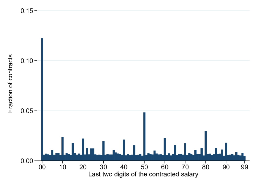
Panel A. Last two digits

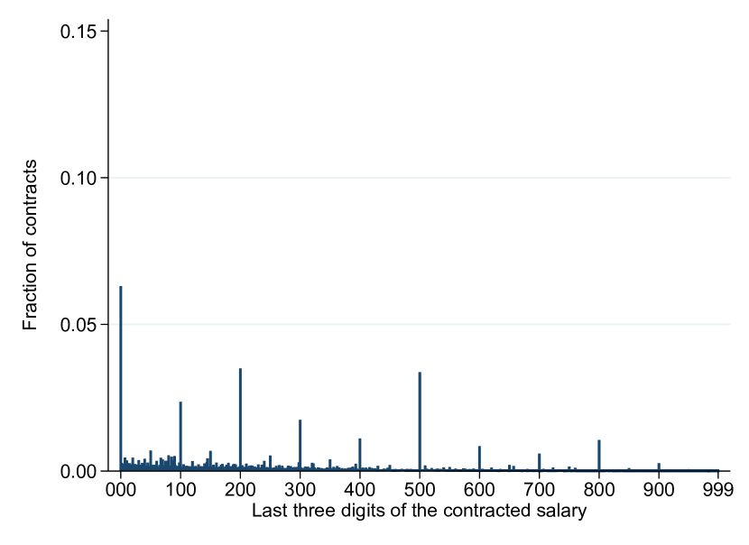
Panel B. Last three digits

Notes: Panel A shows the distribution of the last two digits of contracted earnings (in R$1 bins) in the new-hires sample. Panel B shows the distribution of the last three digits (conditional on the salary having more than three digits).

Figure A2: Distribution of monthly earnings in four Brazilian datasets

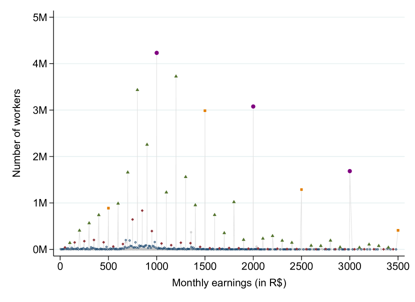
Panel A. Household Survey (PNAD)

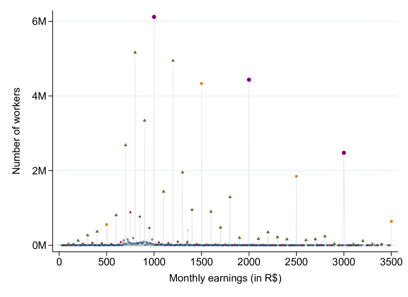
Panel B. Labor Force Survey (PME)

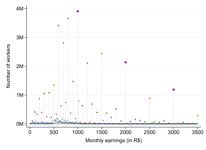
Panel C. Population Census

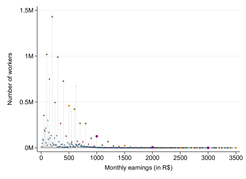
Panel D. Social Programs Registry

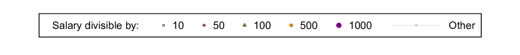
Notes: This figure shows the distribution of monthly earnings in the dataset listed in the panel title. The datasets are the 2013 Brazilian Household Survey (Pesquisa Nacional por Amostra de Domicílios, abbreviated PNAD), the 2013 Brazilian Labor Force Survey (Pesquisa Mensal de Emprego, abbreviated PME), the 2010 Brazilian Population Census (Censo Demográfico), and the 2013 Social Programs Registry of Individuals (Cadastro Único). I focus on the monthly earnings of full-time employed workers aged 18–65. I exclude workers employed by public-sector firms and individuals who work without remuneration.

Figure A3: Histogram of the share of workers hired at a round salary in each firm

Panel A. All firms  

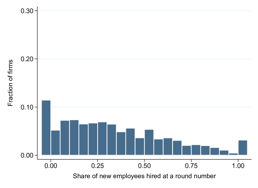
Panel B. Firms that hired five or more workers in the sample

Notes: This figure show histograms of the share of workers in each firm hired at a round-numbered salary in the firm random sample. Panel A shows the histogram for all firms. Panel B shows the histogram for the subset of firms that hired at least five workers during 2003–2017.

Figure A4: Compensation report for an economist in Ithaca, NY, USA

Panel A. Factors that affect the compensation report

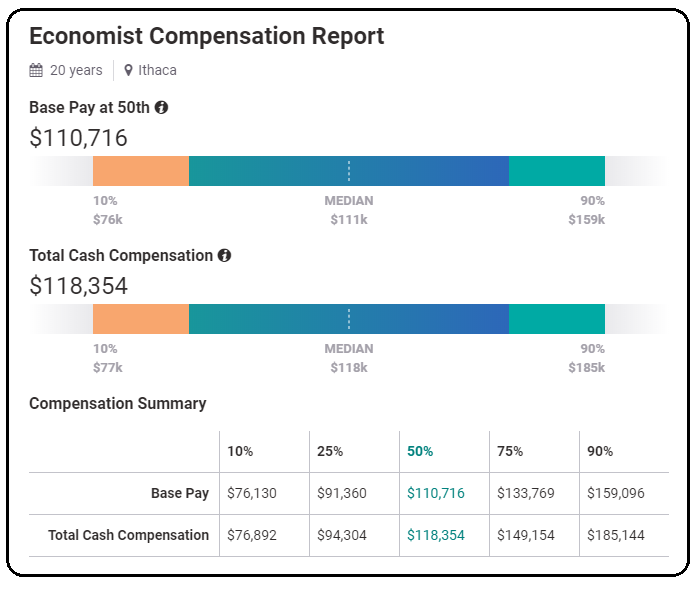
Panel B. Suggested compensation

Notes: This figure shows a compensation report provided by the firm PayScale, based on a query by the author. These compensation reports are advertised as the “right pay” for a prospective candidate.

Figure A5: Wage compression and wage stickiness in the salaries of large firms’ new hires

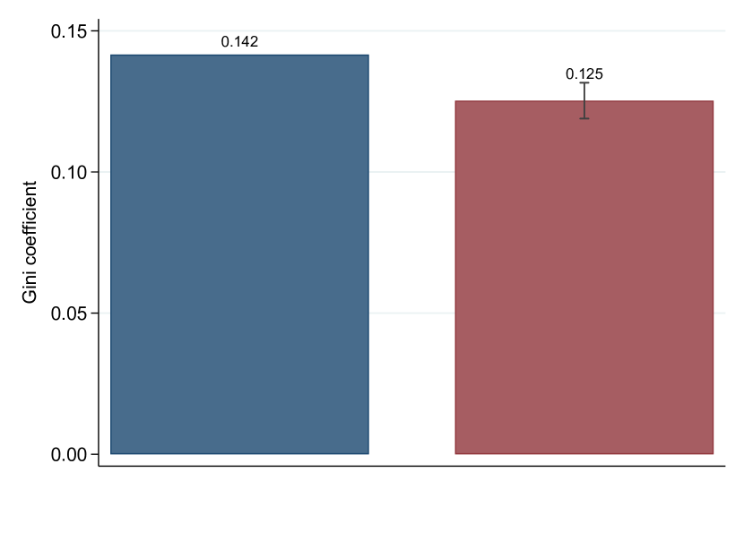
Panel A. Outcome: Gini coefficient

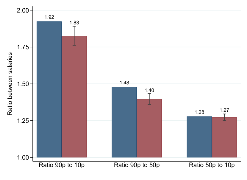
Panel B. Outcome: Percentiles ratios

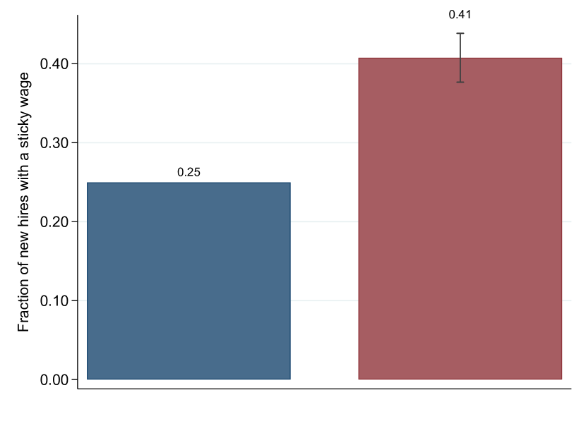
Panel C. Outcome: Initial wage remained constant in nominal terms ratios

Notes: This figure is analogous to Figure LABEL:fig_wage_comp, but the estimates are conditional on firms who, on average across all years in the sample, employ more than five workers. See the notes to Figure LABEL:fig_wage_comp for details on how the figure is constructed, the set of control variables, the definition of the dependent variables, and sample restrictions.

&0.2201.153$-$0.933^∗∗∗2.2282.616$-$0.387^∗∗∗ (0.004)(0.013) Firm age (years)2.2834.981$-$2.698^∗∗∗4.3287.896$-$3.568^∗∗∗ (0.020)(0.145) Has an HR department0.0230.072$-$0.049^∗∗∗0.0890.186$-$0.097^∗∗∗ (0.001)(0.007) Education manager6.5686.626$-$0.057^∗∗∗6.5956.821$-$0.225^∗∗∗ (0.007)(0.037) Average salary (logs)6.4516.523$-$0.072^∗∗∗6.5696.688$-$0.119^∗∗∗ (0.002)(0.013) Notes: This table shows average firm characteristics of bunching firms and non-bunching firms. Bunching firms are defined as firms that hired all new hires at a round-numbered salary in the sample. Large firms are those who employ, on average across all years, more than five workers in the sample. Heteroskedasticity-robust standard errors clustered at the firm level in parentheses. ^∗∗∗, ^∗∗ and ^∗ denote significance at the 1%, 5% and 10% levels.

Notes: This table displays estimates of $\beta$ from equation (LABEL:reg:firm-outcomes), estimated on the subset of firms that employ, on average across years, more than five workers. See notes to Table LABEL:reg_firm_performance for the list of controls and variable definitions. Heteroskedasticity-robust standard errors clustered at the firm level in parentheses. ^∗∗∗, ^∗∗ and ^∗ denote significance at the 1%, 5% and 10% levels.

Notes: This table displays estimates of $\beta$ from equation (LABEL:reg:firm-outcomes). All specifications are estimated at the worker level and include the baseline worker-level controls described in the main text. Additionally, the specifications in this table control for the wage level by including wage fixed effects (in R$100 bins). See notes to Table LABEL:reg_firm_performance for the list of controls and variable definitions. Heteroskedasticity-robust standard errors clustered at the firm level in parentheses. ^∗∗∗, ^∗∗ and ^∗ denote significance at the 1%, 5% and 10% levels.

Bunching firm0.043^∗∗∗0.015^∗∗∗$-$0.016^∗∗∗0.000 (0.004)(0.002)(0.004)(0.002) Mean Dep. Var.0.3530.1150.0160.101 N20,281,31220,281,3121,381,2461,752,411

Panel C. Bunching firm equals one if firm hired over 1/2 workers at a round number     Bunching firm0.012^∗∗∗0.003^∗∗∗$-$0.008^∗∗∗0.004^∗∗∗ (0.001)(0.001)(0.001)(0.001) Mean Dep. Var.0.3530.1150.0160.101 N20,281,31220,281,3121,381,2461,752,411

Panel D. Bunching firm equals one if firm hired over 2/3 workers at a round number     Bunching firm0.017^∗∗∗0.005^∗∗∗$-$0.015^∗∗∗0.007^∗∗∗ (0.001)(0.001)(0.001)(0.001) Mean Dep. Var.0.3530.1150.0160.101 N20,281,31220,281,3121,381,2461,752,411

Panel E. Bunching firm dummy defined using yearly salaries     Bunching firm0.041^∗∗∗0.011^∗∗∗$-$0.039^∗∗∗0.014^∗∗∗ (0.002)(0.001)(0.002)(0.001) Mean Dep. Var.0.3530.1150.0160.101 N20,281,31220,281,3121,381,2461,752,411

Notes: This table displays estimates of $\beta$ from equation (LABEL:reg:firm-outcomes), using several alternative definitions of bunching firms. See notes to Table LABEL:reg_firm_performance for the list of controls and variable definitions. Heteroskedasticity-robust standard errors clustered at the firm level in parentheses. ^∗∗∗, ^∗∗ and ^∗ denote significance at the 1%, 5% and 10% levels.

& No Yes No Yes No Yes Notes: This table displays estimates of $\beta$ from equation (LABEL:reg:firm-outcomes), estimated on the subset of firms that employ, on average across years, more than five workers. Even columns exclude new hires whose salary did not change in nominal terms. See notes to Table LABEL:reg_salary_increase for the list of controls and variable definitions. Heteroskedasticity-robust standard errors clustered at the firm level in parentheses. ^∗∗∗, ^∗∗ and ^∗ denote significance at the 1%, 5% and 10% levels.

& No Yes No Yes No Yes Notes: This table displays estimates of $\beta$ from equation (LABEL:reg:firm-outcomes). In addition to the baseline controls, the specifications in this table control for the wage level by including wage fixed effects (in R$100 bins). Even columns exclude new hires whose salary did not change in nominal terms. See notes to Table LABEL:reg_salary_increase for the list of controls and variable definitions. Heteroskedasticity-robust standard errors clustered at the firm level in parentheses. ^∗∗∗, ^∗∗ and ^∗ denote significance at the 1%, 5% and 10% levels.

Bunching firm0.277^∗∗∗0.246^∗∗∗0.249^∗∗∗0.174^∗∗∗0.274^∗∗∗0.274^∗∗∗ (0.005)(0.008)(0.005)(0.006)(0.005)(0.008) Mean Dep. Var.0.3540.1230.3440.1100.4210.214 N4,953,7823,646,4794,953,7823,646,4794,953,7823,646,479

Panel C. Bunching firm equals one if firm hired over 1/2 workers at a round number     Bunching firm0.178^∗∗∗0.209^∗∗∗0.066^∗∗∗0.045^∗∗∗0.177^∗∗∗0.212^∗∗∗ (0.002)(0.002)(0.002)(0.001)(0.002)(0.002) Mean Dep. Var.0.3540.1230.3440.1100.4210.214 N4,953,7823,646,4794,953,7823,646,4794,953,7823,646,479

Panel D. Bunching firm equals one if firm hired over 2/3 workers at a round number     Bunching firm0.223^∗∗∗0.262^∗∗∗0.085^∗∗∗0.052^∗∗∗0.217^∗∗∗0.260^∗∗∗ (0.002)(0.002)(0.002)(0.001)(0.002)(0.002) Mean Dep. Var.0.3540.1230.3440.1100.4210.214 N4,953,7823,646,4794,953,7823,646,4794,953,7823,646,479

Panel E. Bunching firm dummy defined using yearly salaries     Bunching firm0.239^∗∗∗0.258^∗∗∗0.118^∗∗∗0.050^∗∗∗0.231^∗∗∗0.259^∗∗∗ (0.003)(0.003)(0.003)(0.002)(0.003)(0.004) Mean Dep. Var.0.3540.1230.3440.1100.4210.214 N4,953,7823,646,4794,953,7823,646,4794,953,7823,646,479

Excl. zero growth No Yes No Yes No Yes Notes: This table displays estimates of $\beta$ from equation (LABEL:reg:firm-outcomes), using alternative definitions of bunching firms. Even columns exclude new hires whose salary did not change in nominal terms. See notes to Table LABEL:reg_salary_increase for the list of controls and variable definitions. Heteroskedasticity-robust standard errors clustered at the firm level in parentheses. ^∗∗∗, ^∗∗ and ^∗ denote significance at the 1%, 5% and 10% levels.

&$-$0.972^∗∗∗$-$0.973^∗∗∗$-$0.943^∗∗∗$-$0.012^∗∗∗$-$0.004^∗∗∗$-$0.005^∗∗∗ (0.034)(0.021)(0.034)(0.001)(0.001)(0.001) Firm hiring experience (logs)$-$0.882^∗∗∗$-$0.876^∗∗∗$-$0.642^∗∗∗$-$0.025^∗∗∗$-$0.023^∗∗∗$-$0.007^∗∗∗ (0.050)(0.042)(0.071)(0.001)(0.001)(0.001)

Measure of coarse salary: Div. by 10 (baseline) Div. by 100          Div. by 1000          Div. by 10 (baseline) Div. by 100          Div. by 1,000         

Notes: This table shows linear correlations between the covariate listed in the row header and the outcome listed in the column header using different measures of coarse salaries. Columns 1 and 4 show the results of the baseline specification, using salaries divisible by 10. Columns 2 and 5 use salaries divisible by 100. Columns 3 and 6 use salaries divisible by 1000.

See notes to Table LABEL:tab_predictions for variable definitions and additional details. Heteroskedasticity-robust standard errors clustered at the firm level in parentheses. ^∗∗∗, ^∗∗ and ^∗ denote significance at the 1%, 5% and 10% levels.

Bunching firm$-$0.016^∗∗∗$-$0.097^∗∗∗$-$0.081^∗∗∗$-$0.006 (0.003)(0.033)(0.019)(0.012) Mean Dep. Var.0.1411.9231.4781.278 N557,112557,112557,112557,112 Notes: This table displays estimates of $\beta$ from equation (LABEL:reg:firm-outcomes). Each column shows the results using a different dependent variable. In column 1, the dependent variable is the Gini coefficient. In column 2, the ratio between the 90th and 10th percentiles of the contracted salary distribution among all the new hires in each firm. In column 3, the ratio between the 90th and the 50th percentiles. In column 4, the ratio between the 50th and 10th percentiles.

I use the firm random sample to estimate all regressions. The regressions are estimated at the firm-by-year level on firms that hired at least two workers in my sample.

The regressions control for firm age, share of employees with completed high school, share of employees with completed college, educational attainment of the firm manager, a dummy for having an HR department, the mean earnings of the firm employees, firm size fixed effects, number of hires fixed effects, and industry-by-microregion-by-year fixed effects.

Heteroskedasticity-robust standard errors clustered at the firm level in parentheses. ^∗∗∗, ^∗∗ and ^∗ denote significance at the 1%, 5% and 10% levels.

Appendix B Empirical Appendix

B.1 Informality in Brazilian Labor Markets

International organizations define informality in two main ways. Under the legal definition, a worker is considered to be employed by the informal sector if she does not have the right to a pension when retired. Under the productive definition, a worker is considered informal if (i) she is a salaried worker in a small firm (i.e., a firm that employs fewer than five workers), (ii) a non-professional self-employed, or (iii) a zero-income worker. The share of informal-sector workers in Brazil during 2013 was 35.9% under the legal definition and 43.7% according to the productive definition. Table B.1 shows summary statistics on workers in the national household survey (PNAD), which includes information on workers employed in the informal sector.

Table B1: Summary statistics of workers in the RAIS and the PNAD during 2013

	RAIS		Household Survey (PNAD)
	All workers		All workers		Legal definition			Productive definition
					Formal	Informal		Formal	Informal
	(1)		(2)		(3)	(4)		(5)	(6)
Panel A. Workers’ characteristics
Average age	34.916		38.169		37.548	39.277		36.673	40.096
Male	0.573		0.568		0.563	0.576		0.580	0.552
White	0.581		0.469		0.523	0.372		0.525	0.396
Elementary school or less	0.336		0.481		0.362	0.693		0.313	0.698
Complete high school	0.508		0.390		0.463	0.261		0.472	0.285
Complete university	0.156		0.129		0.176	0.046		0.215	0.017

Panel B. Earnings Mean monthly salary (Reals) 1367.062 1350.902 1416.779 1125.241 1534.599 963.886 Median monthly salary (Reals) 803.923 833.073 833.073 694.228 902.496 694.228

Panel C. Industry Primary sector 0.041 0.127 0.050 0.267 0.014 0.274 Manufacturing 0.136 0.129 0.155 0.082 0.176 0.068 Construction and utilities 0.135 0.156 0.143 0.181 0.149 0.166 Retail 0.264 0.223 0.227 0.216 0.223 0.223 Services 0.424 0.364 0.425 0.255 0.437 0.270

Panel D. Region North 0.055 0.078 0.057 0.116 0.062 0.099 Northeast 0.176 0.252 0.183 0.374 0.197 0.323 Southeast 0.503 0.432 0.491 0.328 0.487 0.362 South 0.172 0.159 0.186 0.110 0.174 0.140 Midwest 0.093 0.079 0.082 0.072 0.081 0.076

Observations (weighted) 68,589,569 87,446,610 56,021,547 31,425,063 49,218,392 38,228,218 Observations (unweighted) 68,589,569 156,432 98,307 58,125 86,631 69,801

Notes: This table shows summary statistics of workers in the Relação Anual de Informações Sociais (RAIS) and the Pesquisa Nacional por Amostra de Domicílios (PNAD), both during 2013. I restrict the PNAD sample to employed individuals aged 18–65. This excludes individuals out of the labor force and unemployed.

Workers in the RAIS (column 1) are slightly younger, more educated, more likely to live in the Southeast (the wealthiest region), have higher earnings, and are significantly less likely to work in the primary sector than workers in the PNAD (column 2). Workers in the RAIS resemble workers in the formal sector of the PNAD (columns 3 and 5). As noted above, this is because informal-sector workers are not included in the RAIS.

B.2 A Potential-Outcomes Framework to Interpret the Reduced-Form Results

In this Appendix, I present a simple potential-outcomes framework to organize the empirical results presented in Section LABEL:sec:firm-behavior.

Let $Y_{j}$ be an outcome of firm $j$ (e.g., profits) and let $B_{j}\in\{0,1\}$ denote an indicator for hiring workers only at round-numbered wages. The observed outcome of a firm can be written as

$$Y_{j}=Y_{0,j}+(Y_{1,j}-Y_{0,j})B_{j},$$ (B1)

where $Y_{0,j}$ and $Y_{1,j}$ are firm $j$’s potential outcomes. $Y_{0,j}$ is the firm’s outcome had it not paid round-numbered wages, regardless of the wages it actually paid; and $Y_{1,j}$ is the firm’s outcome if it pays round-numbered wages.

The observed difference in mean outcomes between firms that pay round-numbered wages (“bunching firms”) and non-bunching firms can be decomposed into two terms as follows:

$$\operatorname{\mathbb{E}}[Y_{j}|B_{j}=1]-\operatorname{\mathbb{E}}[Y_{j}|B_{j}=0] =\underbrace{\left(\operatorname{\mathbb{E}}[Y_{1,j}|B_{j}=1]-\operatorname{\mathbb{E}}[Y_{0,j}|B_{j}=1]\right)}_{\text{Term 1: Causal effect}}$$

$$+\underbrace{\left(\operatorname{\mathbb{E}}[Y_{0,j}|B_{j}=1]-\operatorname{\mathbb{E}}[Y_{0,j}|B_{j}=0]\right)}_{\text{Term 2: Selection bias}}.$$ (B2)

The first term in the right-hand-side of equation (B.2), $\operatorname{\mathbb{E}}[Y_{1,j}|B_{j}=1]-\operatorname{\mathbb{E}}[Y_{0,j}|B_{j}=1]$, represents the causal effect of paying a round-numbered wage for bunching firms. If bunching firms pay new hires a round-numbered wage to exploit a worker bias, we would expect this term to be positive, meaning that exploiting a bias would lead bunching firms to have better outcomes. Conversely, if bunching firms are misoptimizing and doing so is costly, the causal effect would be negative.

The second term, $\operatorname{\mathbb{E}}[Y_{0,j}|B_{j}=1]-\operatorname{\mathbb{E}}[Y_{0,j}|B_{j}=0]$, represents the selection bias. This term captures possible differences in average outcomes between bunching and non-bunching firms, when both types of firms offer non-round-numbered wages. What sign should we expect for the selection bias? Recognizing the existence of a worker bias and implementing a pricing strategy that exploits this bias demonstrates high sophistication. Typically, more sophisticated firms have better outcomes than less sophisticated firms. This can be attributed to, for instance, more effective management practices, which leads to better outcomes (bloom2013does). Consequently, if bunching firms are paying a round-numbered wage to exploit a worker bias, we should expect the selection bias to be positive.

In Section LABEL:sec:firm-behavior, I show that—conditional on a large set of covariates—bunching firms experience worse outcomes than non-bunching firms. This means that the sum of the causal effect and the selection bias is negative. Thus, at least one of the two terms must be negative. If the causal effect is negative, bunching firms are misoptimizing. If the causal effect is non-negative, it follows that the selection bias is negative. But this contradicts the idea that bunching firms are offering round wages because they are sophisticated enough to exploit a worker bias. Thus, the results indicate that the wage-setting strategy of bunching firms is not driven by these firms trying to exploit a worker bias.

Appendix C Theoretical Appendix

C.1 Canonical Wage-setting Models in Labor Economics

There are two broad classes of wage-determination models. The first class of models is wage-posting models. In these models, firms choose what wage to post to maximize profit, in which the optimal wage depends on the worker’s productivity and the firm’s market power, as measured by the elasticity of labor supply. If both worker productivity and firm market power have smooth distributions, then wages should display no bunching. The textbook model of competitive labor markets—in which firms hire workers up to the point that the marginal product of labor equals the market-determined wage—is a special case of wage-posting models. In perfectly competitive models, firms cannot pay a wage below the equilibrium one since no worker would join the firm. Likewise, firms have no incentive to pay a wage above the equilibrium wage. Therefore, in this framework, there is a unique wage determined in equilibrium. Differences in wages across firms and industries might exist due to compensating differentials that arise from job amenity differences. However, as long as these differentials are smoothly distributed across firms, the resulting wage distribution should also be smooth.

The second class of models is wage-bargaining or search-match models. Central to these models are search frictions. The canonical search model is the McCall model (mccall1970economics). In this model, job offers are characterized by a wage, which is the realization of a random variable distributed according to some exogenous distribution. Since firms offer every possible value in the support of the (exogenous) wage distribution, the resulting distribution of wages is smooth. More generally, in wage-bargaining models, firms match with workers and each match generates a surplus that is divided between the firm and the worker. The amount of surplus workers capture in the form of wages depends on their bargaining power. As long as bargaining power is smoothly distributed across workers, there should not be bunching in the wage distribution.

The following section presents a model that can account for the bunching of wages at round numbers observed in the data.

C.2 Setup of the Model

Consider an economy populated by firms using a linear production technology. Firms face an upward-sloping labor supply curve, $l(w)$. The positive slope of the labor supply means that firms have to increase the wage they offer to increase the probability that a worker will accept the offer. Let $p$ be worker productivity and for now assume that the firm observes $p$. Each time the firm wants to hire a worker, the firm’s problem is to choose the wage offer $w$ that maximizes profit

$$\pi=l(w)(p-w).$$ (C1)

C.2.1 Market equilibrium in the frictionless model.

Before introducing optimization frictions, consider first the solution of the standard frictionless model. Suppose workers are randomly matched to firms. In an interior solution, the profit-maximizing wage is

$$w^{*}=p\frac{\eta}{1+\eta},$$ (C2)

where $\eta\equiv l^{\prime}(w^{*})\frac{w^{*}}{l(w^{*})}$ is the elasticity of labor supply. Equation (C2) is the standard solution of the frictionless wage-posting model. This equation tells us that the firm pays workers a fraction $\frac{\eta}{1+\eta}$ of their productivity and earns a profit equal to $\pi(w^{*})=\frac{p}{1+\eta}l(w^{*})$. As $\eta$ increases, workers get compensated for a higher fraction of their productivity. In the limit, as $\eta\to\infty$, we get the standard solution of competitive markets: firms pay workers their productivity ($w^{*}=p$) and earn zero profits. For simplicity, I will refer to $w^{*}$ as the “fully-optimal wage,” although it is optimal only insofar there are no optimization costs.

The shape of the wage distribution in the frictionless model depends on the distribution of market-power-adjusted productivity, $\tilde{p}\equiv p\frac{\eta}{1+\eta}$, across firms. Let $F_{w}$ be the cumulative distribution function (CDF) of observed wages and $F_{\tilde{p}}$ the CDF of $\tilde{p}$. Then,

$$F_{w}(w)=\Pr(w^{*}\leq w) =\Pr\Big{(}p\frac{\eta}{1+\eta}\leq w\Big{)}=F_{\tilde{p}}(w).$$ (C3)

Equation (C3) indicates that, if $F_{\tilde{p}}$ is a smooth distribution, then the distribution of observed earnings, $F_{w}(w)$, is also smooth.

C.2.2 Introducing optimization frictions.

I depart from the standard formulation by modeling coarse wage-setting as a consequence of optimization frictions. I assume that firms’ initial estimate of the fully-optimal wage is a coarse round-numbered wage, $w_{r}$. For example, $w_{r}$ might be the fully-optimal wage rounded to the nearest 1,000. I also assume that firms can pay an optimization cost to learn the fully-optimal wage $w^{*}$. While these assumptions should not be viewed as a perfect description of firm behavior—but rather as useful approximations—they are consistent with evidence from numerical cognition research reviewed in Section LABEL:sub_psych.

Departing from the fully-optimal wage is costly. When the firm offers a coarse wage above the fully-optimal wage ($w_{r}>w^{*}$), the probability that a worker will accept the job offer is higher than the one under the fully-optimal wage, i.e., $l(w_{r})>l(w^{*})$. This leads to the firm hiring workers faster than what would take them if they offered the fully-optimal wage and paying them a wage higher than is optimal. Symmetrically, when a firm offers a coarse wage below the fully-optimal one ($w_{r}<w^{*}$), the firm will be slow to hire workers and the workers will receive a lower wage than is optimal.

Firms will compute $w^{*}$ when they believe it is profitable to do so, namely, whenever the profit gain from computing the fully-optimal wage exceeds the optimization cost. The expected profit difference between paying the fully-optimal and the coarse wage is

$$G(\cdot) \equiv\operatorname{\mathbb{E}}[\pi(w^{*})]-\operatorname{\mathbb{E}}[\pi(w_{r})]$$

$$=(p-w^{*})l(w^{*})-(p-w_{r})l(w_{r}).$$ (C4)

where the expectation is taken over the possible realizations of worker productivity. A first-order Taylor approximation of $l(w_{r})$ around $w^{*}$ yields

$$l(w_{r})\simeq l(w^{*})+l^{\prime}(w^{*})(w_{r}-w^{*}).$$ (C5)

Plugging (C5) back into (C.2.2) and using the FOC, we can write the gain function as follows

$$G(\cdot) \simeq(p-w^{*})l(w^{*})-(p-w_{r})\Big{(}l(w^{*})+\frac{l(w^{*})}{p-w^{*}}(w_{r}-w^{*})\Big{)}$$

$$=pl(w^{*})\frac{\eta^{2}}{1+\eta}\Big{(}\frac{w_{r}-w^{*}}{w^{*}}\Big{)}^{2}$$

$$=\pi(w^{*})\eta^{2}\tilde{w}^{2},$$ (C6)

where $\tilde{w}\equiv\frac{w_{r}-w^{*}}{w^{*}}$ is the percentage deviation of $w_{r}$ about $w^{*}$ or the wedge between the optimal and the round-numbered wage.

The firm will optimize whenever the profit gain (given by equation (C.2.2)) is greater than the optimization cost. I assume that firms have to forego a fraction $\tau$ of their profits to optimize. Hence, firms fully optimize whenever $\eta^{2}\tilde{w}^{2}\geq\tau$.

C.2.3 Heterogeneity in the optimization cost.

Suppose that the optimization cost $\tau$ is heterogeneously distributed across firms according to the CDF $F_{\tau}$. The probability that a firm will offer a coarse wage is

$$\theta =\Pr\Big{(}\tau>\eta^{2}\tilde{w}^{2}\Big{)}=1-F_{\tau}\Big{(}\eta^{2}\tilde{w}^{2}\Big{)}.$$ (C7)

Using equation (C7), one can characterize the distribution of observed wages in the model with frictions. A fraction $\theta$ of workers are hired at a coarse round-numbered wage. The remaining workers are hired by firms that optimize according to the distribution of the fully-optimal wage, $F_{\tilde{p}}$. The CDF of observed wages, $F_{w}$, is a convex combination of the distribution of the fully-optimal wage, $F_{\tilde{p}}$, and the distribution of the coarse round-numbered wage, $F_{w_{r}}$, with mixture weight $\theta$:

$$F_{w}=\theta F_{w_{r}}+(1-\theta)F_{\tilde{p}}.$$ (C8)

Consistent with the data, the distribution of observed wages in the model with frictions exhibits bunching at $w_{r}$. The size of the bunching is given by the fraction of workers hired through coarse wage-setting, $\theta$. The standard wage-posting model is a special case of the model with optimization frictions, in which $\tau=0$ (which implies $\theta=0$).

C.3 Optimization with Varying Degrees of Precision

The baseline model with frictions assumes that the decision of the firm is binary: the firm either offers a wage equal to $w_{r}$ or pays an optimization cost and offers the fully-optimal wage, $w^{*}$. In this subsection, I extend the model to incorporate different degrees of precision in refining the initial estimate of the fully-optimal wage. In the generalized model, the wage distribution exhibits bunching at multiple round numbers. The size of the bunching at each round number reflects the relative marginal benefit and cost of making a better approximation to the fully-optimal salary.

Without loss of generality, assume that wages can have at most four digits. Suppose, furthermore, that the firm’s initial estimate of the fully-optimal wage is such a wage rounded to the coarsest round number. In this case, the fully-optimal wage rounded to the nearest 1,000, $w_{1000}$. By paying $\tau_{100}$, they can learn the second digit of the optimal wage and offer the optimal wage rounded to the nearest 100, $w_{100}$. After learning the second digit, the firm can pay $\tau_{10}$ to learn $w_{10}$, the optimal wage to the nearest ten, and finally, pay $\tau_{1}$ to learn exactly the fully-optimal wage.

To illustrate the trade-offs faced by the firm, Appendix Figure C1 plots a firm’s profit as a function of the wage posted. The fully-optimal wage (ex-ante unknown to the firm) is at point A. Without loss of generality, suppose that $w_{1000}<w^{*}$ is the firm’s initial estimate of the fully-optimal wage, shown at point B (i.e., the fully-optimal wage rounded to the nearest 1,000). The firm could forfeit a fraction $\tau_{100}$ of its profits to compute the second digit of the optimal wage and learn $w_{100}$ (i.e., the optimal wage up to the nearest 100), shown at point C. The firm will do so as long as $\frac{\pi(w_{100})}{\pi(w_{1000})}\geq\frac{1}{1-\tau_{100}}$.

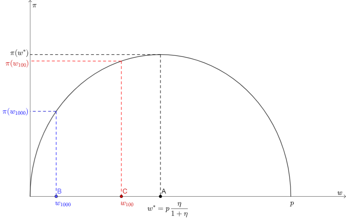
Figure C1: Firm’s profit as a function the worker’s optimal wage

Notes: This figure illustrates the problem of a firm deciding how many digits of a worker’s fully-optimal wage to learn. The figure plots the profit of the firm as a function of the wage posted. The optimal wage of the frictionless model, $w^{*}$, is ex-ante unknown to the firm and shown in . For illustration purposes, the figure displays the case in which $w_{1000}<w^{*}$ is the firm’s initial estimate of the fully-optimal wage (point ). The firm can forego a fraction $\tau_{100}$ of its profits to compute the second digit of the optimal wage (i.e., the optimal wage up to the nearest hundred) and learn $w_{100}$, shown in point . The firm will do so as long as $\pi(w_{100})(1-\tau_{100})\geq\pi(w_{1000})$.

The firm will continue refining its estimate of the fully-optimal salary as long as the marginal benefit of learning an additional digit is greater than the marginal optimization cost. Observe that learning further digits of the fully-optimal wage shrinks the mispricing wedge at a decreasing rate. If the initial estimate is equal to the fully-optimal wage up to the nearest 1,000, the error from not learning the second digit is at most 500, the error from not learning the following digit is at most 50, and the error from not learning the final digit is at most 5.

Let $\theta_{1000}$, $\theta_{100}$, and $\theta_{10}$ be the fraction of workers hired at coarse wages divisible by 1,000, 100, and 10, respectively. The distribution of observed wages in this model has the following mixing distribution:

$$F_{w}=\sum_{\mathclap{j\in\{10,10^{2},10^{3}\}}}\theta_{j}F_{w_{j}}+(1-\sum_{\mathclap{j\in\{10,10^{2},10^{3}\}}}\theta_{j})F_{\tilde{p}}.$$ (C9)

Equation (C9) is the generalization of equation (C7) for the case in which firms learn with different degrees of precision. In this case, we observe bunching at several round numbers. The size of the bunching at each round number reflects the fact that different firms learn a different number of digits, depending on how costly it is to do so and how much they stand to gain.

Appendix D Data Appendix

D.1 Worker Record Booklet and RAIS Orientation Handbook

The main variable in the analysis is the contracted salary of each new hire. The contracted salary is the salary contained in the worker record booklet (CTPS). The CTPS lists the employment record of all workers employed in the formal sector and includes information on the worker’s admission date, initial salary, and salary increases. Appendix Figure D1 shows an example of a worker record booklet and the information contained in it.

Figure D1: Example of a worker record booklet or CTPS

There are good reasons to believe that workers’ contracted salary is accurately measured in the RAIS. First, firms have available an orientation handbook that details how to complete the information required by the RAIS. The following box shows an English translation of the section that explains how to complete the information regarding the contracted salary, taken from the 2019 orientation handbook (p.p. 29-30).

In addition to the handbook, there are several online resources that provide further assistance. Appendix Figure D2 exhibits an example of a publicly-available video that explains how to complete the contracted salary section of the RAIS.

Figure D2: Video explaining how to complete RAIS contracted salary information

Notes: Source is RAIS 2017 – Como Informar o Salário Contratual?

D.2 Variable Definitions

This section describes the variables that I use in the regressions presented in Sections LABEL:sec:firm-behavior and LABEL:sec:implic.

• Educational attainment of the firm manager. This variable measures the schooling level of the highest-ranking person in each firm. I first assess if a firm has a chief executive officer (CEO). To identify a firm’s CEO, I use the Brazilian occupational code classification (Classificação Brasileira de Ocupações, or CBO for short). The CBO identifies CEOs with the code 121010. If a firm does not employ any worker with this code, I use the educational attainment of the managers of the firm (identified by a first CBO-digit equal to one) and supervisors (identified by the third CBO-digit equal to zero). In case the firm has no managers or supervisors, I define the highest-ranking person in each firm as the worker with the highest wage.

• Firm age. This variable measures the number of years since the firm was created. I do not directly observe the firm creation date in the data. I proxy the foundation year as the minimum between (i) the first year in which the firm appears in the RAIS (using data since 1995) and (ii) the oldest admission year among all workers employed by the firm. I calculate the firm age as the difference between the current year and the firm creation year.

• Firm size growth. This variable measures the growth rate in the firm’s number of employees. To compute this measure, I calculate the percent change in the number of workers employed by each firm between consecutive years.

• Firm survival rate. This variable indicates whether the firm exited the market. I identify a firm as exiting the market if it does not have any active workers at the end of the year.

• Has a human resources department. This variable indicates whether a firm has a human resources (HR) department. I identify firms as having an HR department if one of its employees is an HR manager (CBO codes 123205, 123210, 142210,142205) or an HR support staff (CBO codes 252105, 252405, 411030).

• Mean earning of firm employees. This variable measures the average earnings of a firm’s workers in a given year. I use workers’ average monthly salary throughout a year as the relevant earnings measure and compute the average of this measure across all workers. I use the yearly consumer price index (CPI) to express earnings in real terms.

• New hire separated. This variable measures whether a new hire separated from the firm during the year the worker was hired or the following year. This variable is equal to one if a new hire is not employed at the end of the hiring year or at the end of the following year and is equal to zero if the new hire remains employed at the end of both years.

• New hire resigned. This variable is computed analogously to the one that measures new hires’ separation, but using resignations (i.e., worker-initiated separations) instead of overall separations.

• Number of hires. This variable measures the number of workers hired by the firm during 2003–2017. To compute this variable, I only consider hires with a monthly contract and hired at a salary above the federal minimum wage. This sample restriction makes the analyses of the firm random sample comparable to the analyses of the new-hires sample.

• Ratio between percentiles of the new hires’ salary distribution. This variable measures the ratio between salaries in different percentiles of the contracted salary distribution among the new hires of a given firm during 2003–2017. Before computing the ratio, I adjust all salaries using the yearly CPI. I winsorize the ratios at the 99th percentile.

• Salary increase in percent is an integer. This variable indicates whether the percent salary increase of a worker is an integer number. To compute this measure, I calculate the percent change in workers’ contracted salary between the year the firm hired the worker and the following year. The indicator variable is equal to one if the percent change is an integer and zero otherwise.

• Salary increase in Brazilian Reals is a round number. This variable indicates whether the salary increase of a worker, measured in Brazilian Reals, is divisible by ten. To compute this measure, I calculate the difference in a worker’s contracted salary between the year the worker was hired and the following year. The indicator variable is equal to one if this difference is a round number and zero otherwise.

• Share of employees with completed high school. This variable measures the fraction of a firm’s employees that completed at least high school. To compute this variable, I first calculate the number of workers in each firm with educational data available over the 2003–2017 period. Next, I compute the number of workers who finished high school over the same period. Finally, I compute the ratio between these two variables.

• Share of employees with completed college. This variable is computed analogously as the share of employees with completed high school.

• Worker contracted salary. The contracted salary represents a worker’s salary as per the worker’s contract at the end of each year. For a new hire, the contracted salary is the same as the initial salary. For other workers, the contracted salary is equal to the current salary, which might differ from the initial salary due to promotions or other wage adjustments.

D.3 Measurement Error in the Contracted Salaries of 2016 and 2017

In the 2016 and 2017 RAIS, the contracted salary variable contains substantial measurement error. The RAIS reports two measures of a worker’s contracted salary that are equivalent before 2016:

• The first measure is the contracted salary in Brazilian Reals. This is the variable that I use throughout the paper.

• The second measure is the contracted salary measured in multiples of the federal monthly minimum wage.

In 2016 and 2017, these two measures are not equivalent. Half of the workers earn monthly salaries below the minimum wage according to the contracted salary in Reals but earn salaries above the minimum wage according to the second measure. Upon further exploration, it appears that many firms reported their employees’ earnings in units of hundreds of Brazilian Reals. In other words, for many workers, the contracted salary reported in multiples of the minimum wage is equal to the contracted salary reported in Reals divided by the minimum wage and multiplied by 100. I adjusted the reported earnings for these workers to correct this discrepancy. Excluding 2016 and 2017 from the analysis does not change the main results of the paper.

D.4 Sample Restrictions

In this section, I describe the sample restrictions that I impose on the new-hires sample. Appendix Table LABEL:tab_metadata shows the number of observations (contracts) at the beginning and at the end of each step of the data cleaning process. The analysis begins in 2003 since this is the first year in which the characteristics of workers’ contracts are available in the RAIS.

1. I include only new hires in each year. I exclude the contracts of workers hired during previous years to avoid double-counting the same worker.

2. I only consider workers with a valid identifier. Workers in the private sector are uniquely identified by their ID in the Social Integration Program (PIS, for its name in Portuguese, Programa de Integração Social). The eleven-digit PIS ID of a worker is constant throughout the worker’s career. I only keep workers with an eleven-digit ID.

3. I exclude workers employed by public-sector firms.

4. I only consider workers hired at a monthly contract. In the sample, about 91% of contracts are signed at the monthly level. The second most common type of contract is at the hourly level (about 7.5% of all contracts).

5. Some firms report hiring workers at a salary below the federal montly minimum salary. This is likely due to measurement error. To deal with this, I drop all the contracts that are made for earnings below the federal monthly minimum salary of each year.

6. Some firms report hiring the same worker multiple times in a given year. I only keep one observation per worker-firm-year.

7. I exclude new hires for whom their contracted wage is missing.

At the end of this process, I remain with data on over 210 million contracts. I group workers in R$1 bins (roughly 30 cents of a dollar) and winsorize the right tail of the distribution at R$10,100 (this affects about 0.3% of the workers).

934,129,652 763,396,508 49,580,874 0.333 0.332 0.276 0.242 0.234 0.227 0.227 211,854,662 185,223,774 25,483,030

Notes: This table shows the number of contracts, unique workers, and unique firms in each year before and after imposing the sample restrictions. See text for a description of each sample restriction.

Appendix E Estimating a Counterfactual Earnings Distribution

In this Appendix, I explain how I construct a counterfactual earnings distribution that does not feature bunching at round-numbered wages.

The standard approach to construct a counterfactual distribution in the bunching literature involves estimating a high-degree polynomial on the observed earnings distribution excluding the salaries that exhibit bunching and using the estimated polynomial coefficients to predict the counterfactual number of workers at the salaries where workers bunch.

The first step consists of regressing the number of workers in bin $b$, $C_{b}$, on a function $f(\cdot)$ that depends on the earnings of bin $b$, $w_{b}$,

$$C_{b}=\alpha+f(w_{b})+\varepsilon_{b}.$$ (E1)

Previous work has traditionally set $f(\cdot)$ as a high-degree parametric function of earnings, including dummy variables at the salaries of the distribution that exhibit bunching. A straightforward implementation of this approach would be to set

$$f(w_{b})=\sum_{p=1}^{P}\beta_{p}(w_{b})^{p}+\sum_{r\in R}\gamma_{r}\mathbbm{1}{\{w_{b}=r\}},$$

where $\sum_{r\in R}\gamma_{r}$ is a set of dummies, one for each round number, and $P$ is the polynomial degree. The counterfactual distribution without bunching is estimated using the predicted values from (E1), omitting the contribution of the dummies

$$\hat{C_{b}}=\hat{\alpha}+\sum_{p=1}^{P}\hat{\beta}_{r}(w_{b})^{p}.$$ (E2)

This parametric approach is well-suited to estimate counterfactual distributions locally, that is, around one particular kink or notch. However, I need to estimate a counterfactual density around each round number. As I show below, the parametric approach tends to perform poorly in estimating global counterfactuals.

An appealing alternative is to use a non-parametric approach. I estimate kernel-weighted local polynomial regressions using a uniform kernel on non-round-numbered earnings and use the estimates to predict the density at round-numbered wages. Intuitively, to estimate the density at each salary, I use data points “close” to the salary, where close is defined by the bandwidth of the kernel. For a sufficiently large bandwidth (i.e., a bandwidth that covers the entire support of the earnings distribution), the local polynomial regression yields the exact same counterfactual as the parametric one. However, for a small bandwidth, the non-parametric approach yields better-behaved estimates. To see this, Appendix Figure E1 compares the counterfactual distribution of earnings using the parametric and non-parametric approaches, in both cases using a seventh-degree polynomial. Unlike the non-parametric counterfactual distribution, the parametric one yields a negative estimated number of workers in some segments of the distribution.

Since the counterfactual number of observations does not include the contribution of the dummies, the aggregate number of observations in the data, $N$, is necessarily higher than the predicted total number of observations, i.e., $N=\sum_{b}C_{b}>\sum_{b}\hat{C}_{b}=\hat{N}$. To account for this, I re-weight all observations by $\frac{\sum_{b}C_{b}}{\sum_{b}\hat{C}_{b}}$. This approach rules out extensive margin responses. This means that the use of coarse wages moves workers around the earnings distribution, but it does not make any worker leave or enter the labor market altogether. This implies that the excess mass at round-numbered salaries corresponds to missing mass at non-round-numbered salaries.

To quantify the missing mass, I follow kleven2013using and select the narrowest manipulation region consistent with the data. To illustrate how the approach works, Appendix Figure E3 shows how the counterfactual distribution, excess mass (Panel A), and missing mass (Panel B) around R$3000 are estimated.

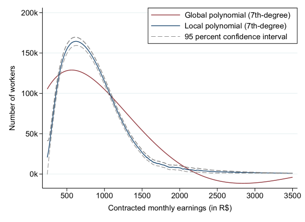
Figure E1: Comparison of parametric and non-parametric counterfactual distributions

Notes: This figure compares the counterfactual earnings distribution using two different approaches. The red line denotes the counterfactual earnings distribution using a global 7th-degree polynomial. The blue line denotes the counterfactual distribution using a local 7th-degree polynomial. The gray dashed line around the local polynomial denotes the 95% confidence interval.

Figure E2: Robustness of the counterfactual distribution to alternative specifications

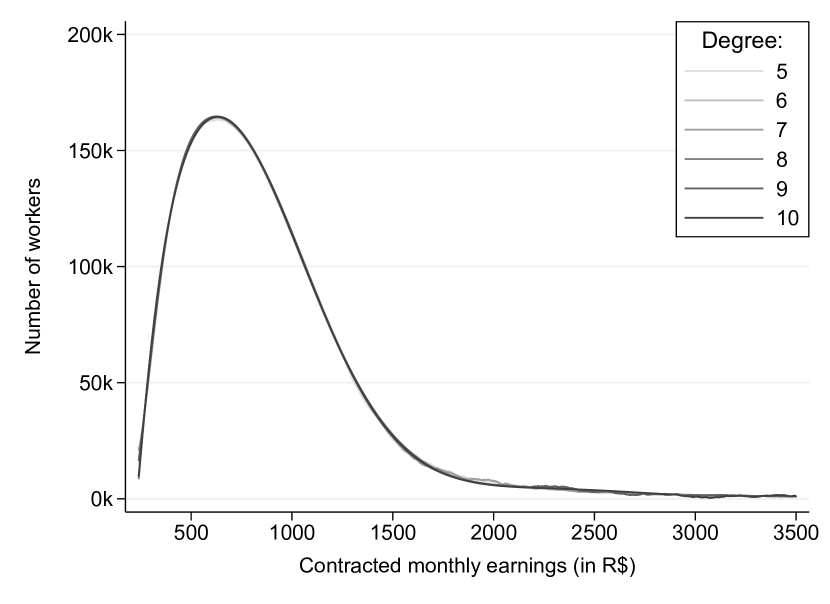
Panel A. Robustness to polynomial degree

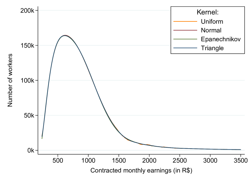
Panel B. Robustness to kernel choice

Notes: This figure shows how the counterfactual earnings distributions estimated using a local polynomial approach changes when varying the polynomial degree (Panel A) and the type of kernel (Panel B). See Appendix E for details on how I estimate the counterfactual distribution.

Figure E3: Estimation of the counterfactual distribution, excess mass, and missing mass

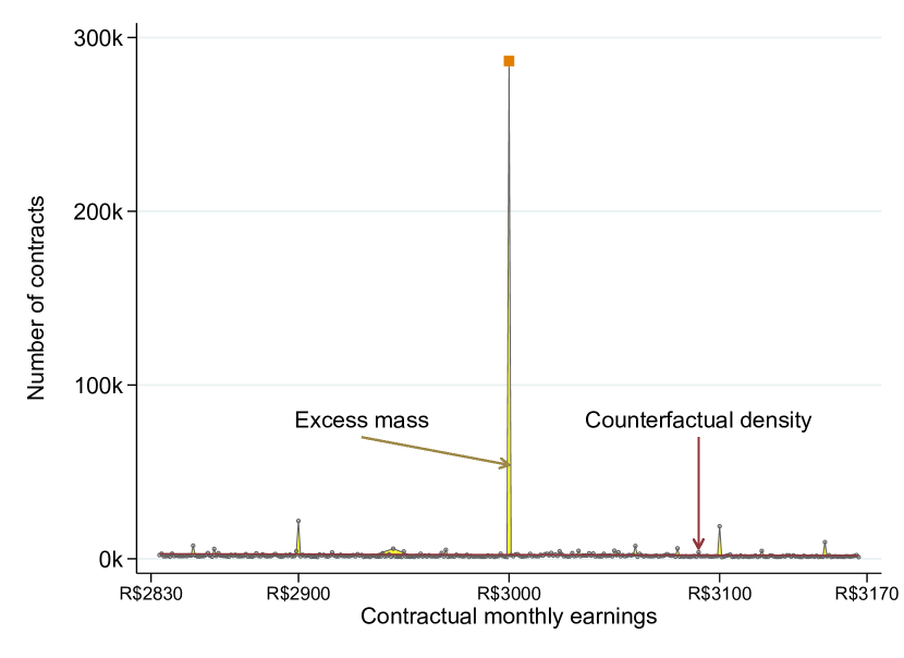
Panel A. Excess mass

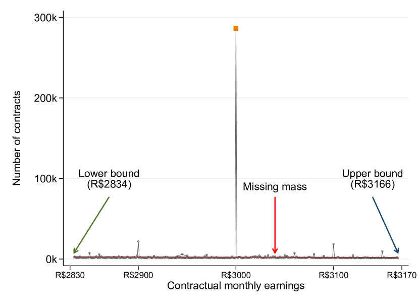
Panel B. Missing mass

Notes: This figure illustrates how I calculate the excess mass at R$3,000. The figure shows the distribution of earnings between R$2,834 and R$3,166 in the new-hires sample. Gray dots denote the observed number of workers, while the red line denotes the counterfactual distribution estimated with a local polynomial. The yellow area in Panel A denotes the excess mass, which is equal in magnitude to the missing mass denoted by the red area in Panel B.

Appendix F Alternative Explanations

In this Appendix, I assess five alternative explanations for the bunching observed in the data. The explanations I discuss are: worker left-digit bias, focal points in wage bargaining, fairness concerns, round wages as a signal of job quality, and changes in marginal tax rates.

F.1 Worker left-digit bias

One possible explanation for the clustering of wages at round numbers is that firms use round salaries as an optimal response to a worker bias. A plausible bias that has been documented in other environments is the left-digit bias, that is, the propensity of individuals to pay more attention to the first digit of a number relative to the other digits (korvorst_differential_2008, lacetera_heuristic_2012, strulov2019more).

I view the results in Section LABEL:sec:firm-behavior as the main evidence against firms paying round-numbered wages as an optimal response to worker left-digit bias. Specifically, I find that firms that are smaller, younger, have less hiring experience, and do not have an HR department are the ones more likely to pay round-numbered salaries to new hires. It is unlikely that these firms are paying round-numbered salaries to exploit a worker bias. Having awareness of a worker bias requires a considerable amount of sophistication, and these firms are less sophisticated in observable characteristics.

For completeness, I conduct two additional tests for worker left-digit bias. As a first test, I analyze whether workers earning just below round salaries have systematically higher separation rates than workers earning exactly a round salary or a salary just above it. This test is analogous to one conducted by dube_monopsony_2020 using observational data. Intuitively, in the presence of a left-digit bias, workers with salaries close to but below a round number would be more likely to leave a firm to pursue a better wage than workers earning a round salary or a salary just above it. A problem with separation rates is that the separations might be driven by firms exiting the market, as opposed to workers leaving because they found a better match. In the data, I observe whether the employer or the employee initiated the separation. Thus, I estimate worker resignation rates (i.e., worker-initiated separations) in the vicinity of round salaries.

As a second test for worker left-digit bias, I analyze whether there is an asymmetric mass of workers just below and just above round salaries. According to some models of left-digit biased workers, most of the excess mass observed at round salaries should come from salaries just below the round number. There are alternative ways of modeling worker left-digit bias, some of which predict that the missing mass also comes from above each round number (e.g., strulov2019more). Thus, while this test is informative of the possible existence of left-digit bias, it is by no means conclusive.

F.1.1 Worker resignation rate  

Visual evidence. Appendix Figure F1, Panel A shows the resignation rate of workers hired at each salary divisible by 100, a salary just below it, and just above it. To construct this figure, I compute the resignation rate for three sets of workers: those who earn a round salary $w_{r}$, those whose earnings fall in the $[w_{r}-h,w_{r})$ range where $h$ is the bandwidth (these are the workers “just below” $w_{r}$), and those who earn a salary in the $(w_{r},w_{r}+h]$ range (these are the workers “just above” $w_{r}$). I calculate the resignation rates in the vicinity of each salary divisible by 100 and for $h=10$.

The average resignation rate of workers earning just above round salaries is equal to the one for workers hired at a salary just below a round number (in both cases, equal to 0.048). In turn, these workers are, on average, slightly less likely to resign relative to workers that earn exactly a round salary. On average across round numbers, the average resignation rate of workers that earn a salary divisible by 100 is 0.051. Moreover, workers earning a round salary have higher resignation rates not just on average, but also for almost every salary divisible by 100. These results are robust to alternative bandwidths.

Regression discontinuity analysis. Next, I use a regression discontinuity (RD) design to assess whether the differences in resignation rates shown above are statistically significant. I estimate regressions of the form:

$$\text{Res}_{i} =\alpha+\nu w_{i}+\beta_{r}\mathbbm{1}{\{w_{i}=w_{r}\}}+\gamma_{r}\mathbbm{1}{\{w_{i}>w_{r}\}}$$

$$+\delta_{r}w_{i}\mathbbm{1}{\{w_{i}>w_{r}\}}+\varepsilon_{i}\hskip 2.84544pt\text{ if }|w_{i}-w_{r}|\leq h,$$ (F1)

where $\text{Res}_{i}$ equals one if worker $i$ resigned and zero otherwise, $w_{i}$ is the contracted salary of worker $i$, $w_{r}$ is a round salary within distance $h$ of $w_{i}$, and $h$ is the bandwidth. The two coefficients of interest are $\beta_{r}$ and $\gamma_{r}$. They measure whether workers earning exactly $w_{r}$ and workers earning just above $w_{r}$, respectively, have differential average resignation likelihoods, relative to workers earning just below $w_{r}$.

Appendix Figure F1, Panel B plots the estimated $\hat{\beta}_{r}$’s and $\hat{\gamma}_{r}$’s for $h=10$. Each coefficient comes from estimating equation (F.1.1) around a different round number divisible by 100. Consistent with the visual evidence, workers earning a round salary are more likely to resign relative to workers with earnings just below or just above one. This is true for most round numbers, although, in some cases, the standard errors are quite large. In contrast, workers earning just above each round salary do not have systematically different likelihoods of resigning than workers earning just below round salaries.

In sum, these results indicate that the workers who earn a round-numbered salary are more likely to resign than workers who earn a salary just below or just above the round number. This provides further evidence against the hypothesis that firms pay round-numbered salaries to exploit worker left-digit bias.

F.1.2 Mass of contracts below and above round salaries  

Visual evidence. Appendix Figure F2, Panel A shows the fraction of workers whose earnings are just below and just above salaries divisible by 100. To construct this figure, I compute the number of workers whose earnings are within a bandwidth $h$ of a round salary $w_{r}$. Specifically, I compute the number of workers whose earnings fall in the range $[w_{r}-h,w_{r})$—these are the workers “just below” $w_{r}$—and in the range $(w_{r},w_{r}+h]$—these are the workers “just above” $w_{r}$. Next, I add up the number of workers just below and just above. Finally, I calculate the fraction of workers that come from each side of the round number. I do this calculation for each salary divisible by 100 and a bandwidth $h=10$.

I find no systematic differences in the number of workers. For some round salaries (e.g., R$500), there are more contracts above the round number, while for other salaries (e.g., R$1,300), the opposite is true.

Regression discontinuity analysis. Next, I use a RD design to formally test whether the number of workers exhibits a statistically significant jump at round salaries. I follow the approach of papers that look for discontinuities in the number of observations around a target value (e.g. camacho2011manipulation). Specifically, I estimate the following regression for each $w_{r}$ divisible by 100:

$$\frac{C_{b}}{N_{b}}=\tilde{\alpha}_{r}+\tilde{\beta}_{r}\mathbbm{1}{\{w_{b}>w_{r}\}}+\tilde{\nu}_{r}w_{b}+\tilde{\delta}_{r}w_{b}\mathbbm{1}{\{w_{b}>w_{r}\}}+\tilde{\varepsilon}_{b}\text{ if }|w_{b}|\leq h\text{ and }w_{b}\neq w_{r},$$ (F2)

where $C_{b}$ is the count of contracts in bin $b$, $w_{b}$ is the salary of the bin, $w_{r}$ is a round salary, $N_{b}$ is the total number of contracts within distance $h$ of $w_{b}$, and $h$ is the bandwidth. The dependent variable is the fraction of contracts in each bin. The coefficient of interest is $\tilde{\beta}_{r}$. It measures whether there is a discontinuity in the fraction of observations in each bin after crossing a round salary $w_{r}$. Some left-digit bias models predict $\tilde{\beta}_{r}>0$.

Appendix Figure F2, Panel B plots the estimated discontinuity $\tilde{\beta_{r}}$ at each salary divisible by 100. Each coefficient comes from estimating equation (F2) for a different round salary. Across round numbers, the point estimates are small, in many cases negative, and always statistically indistinguishable from zero. The results are similar using alternative bandwidths. Taken together, the results of this section show that the difference between the number of workers just above and just below round salaries does not exhibit any systematic pattern, tends to be quantitatively small, and is statistically insignificant.

F.2 Other Alternative Explanations

F.2.1 Focal points in wage bargaining.

If workers and firms bargain over the initial salary and round numbers are focal points in these negotiations, then we might expect to observe bunching at round salaries. hall2012evidence show that wage bargaining is more prevalent across high-wage knowledge workers, whereas wage posting is more frequent in low-wage blue-collar occupations. Therefore, if the bunching were driven entirely by focal points in wage bargaining, we should not expect to observe any bunching in low-wage occupations, where take-it-or-leave-it offers are more prevalent. To test this hypothesis, I estimate the fraction of workers hired at coarse wages across industries and occupations. Appendix Figure F3 shows the results.

Overall, coarse wages are prevalent both across industries where we should expect more wage-posting (such as manufacturing) and more wage-bargaining (such as financial intermediation). Similarly, coarse wages are pervasive across both blue-collar occupations (like administrative workers) and white-collar occupations (like professionals, artists, and scientists). Therefore, focal points in negotiations are unlikely to explain the bunching observed in the data.

F.2.2 Focal points in collective bargaining agreements.

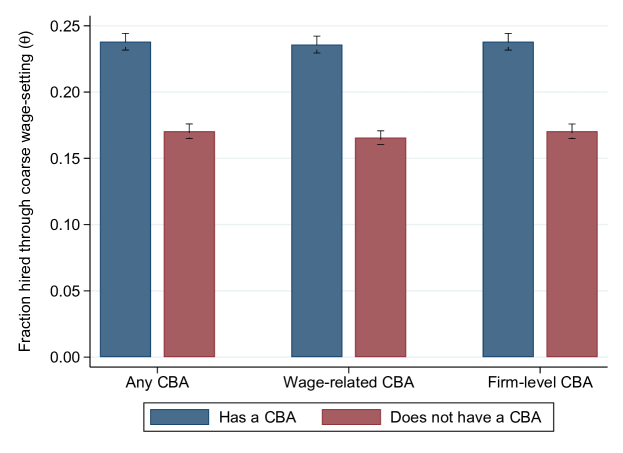
Figure F4: Collective bargaining agreements and fraction of workers hired through coarse wage-setting ($\hat{\theta}$)

The bunching of salaries at round-numbered wages could be explained by round numbers acting as focal points in collective bargaining agreements (CBAs), which are legal contracts between a firm and a union representing the workers. To test this explanation, I use data on the universe of CBAs signed during 2008–2017 (lagos2023labor). For context, 11.7% of the workers in the new-hires sample were hired by firms that signed a CBA, and 9.1% of the workers hired at a round-numbered wage were hired by firms that signed a CBA. I use this data to estimate the fraction of workers hired at coarse wages for firms that signed a CBA and firms that did not sign a CBA. Appendix Figure F4 shows the results.

Coarse wage-setting is prevalent in both firms that signed a CBA (blue bars) and firms without a CBA (red bars). This is true for firms that signed any type of CBA, and also for firms that signed a CBA that includes a wage clause (usually related to wage floors and salary adjustments). Therefore, focal points in CBAs are unlikely to the bunching observed in the data.

F.2.3 Fairness concerns.

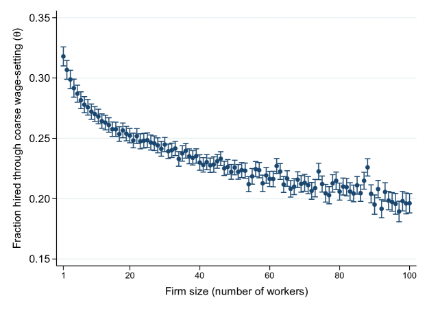
Figure F5: Firm size and fraction of workers hired through coarse wage-setting ($\hat{\theta}$)

Inequity aversion and fairness concerns might induce firms to pay the same salary to coworkers performing the same tasks, even if their productivity is different. By definition, fairness concerns should only matter in firms that employ multiple employees. However, firms with just one employee are the ones most likely to pay coarse wages (Appendix Figure F5).

F.2.4 Round wages as a signal of job quality.

In the consumer market, some high-quality firms price their products at round numbers to signal their quality. Some evidence suggests high-end retailers are more likely to round their prices relative to low-end retailers (stiving_price-endings_2000). In the labor market, firms might also use the roundness of the salary to signal the job’s quality. Crucial to this information-based explanation is that consumers or job-seekers, correspondingly, lack information about the quality of relative products or jobs. Otherwise, there would not be a need to use prices to signal quality. If workers become better at assessing the quality of a job as they gain more experience, we should expect firms hiring more experienced workers to be less likely to bunch. However, this is the opposite of what I find. As worker experience increases, firms are more likely to pay a coarse wage.

F.2.5 Changes in marginal tax rates.

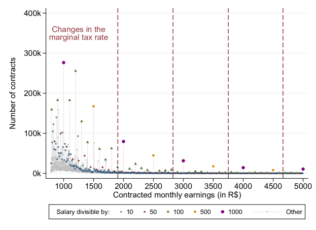
Figure F6: Distribution of contracted salaries and kinks in the income tax schedule during 2015

Beginning with saez_taxpayers_2010, several papers have shown that changes in marginal incentives—particularly, changes in marginal tax rates—can generate bunching. Thus, one possible concern is that the estimate of $\theta$ might be confounded by changes in the marginal tax rate. To assess this, I collected data on all the changes in the personal income tax rate in Brazil from 2007–2015. I find that none of the kink points in this period were at round numbers. Furthermore, there is no detectable bunching at any of the kink points. For example, Appendix Figure F6 shows the distribution of earnings and kink points using data from 2015. For monthly earnings below R$1,903.98, the marginal tax rate is zero. The marginal tax rate jumps to 7.5% for earnings between R$1,903.99 and R$2,826.65 and keeps increasing by 7.5 percentage points at each of the following income thresholds: R$2,826.66, R$3,751.06, and R$4,664.68. There is no bunching at any of these thresholds. The lack of bunching at the kink points is consistent with the findings of saez_taxpayers_2010 and chetty_adjustment_2011, who show that the bunching observed in tax data is driven by the self-employed—who have more scope to manipulate their earnings—rather than wage employees.

Figure F1: Resignation rates below, at, and above salaries divisible by 100

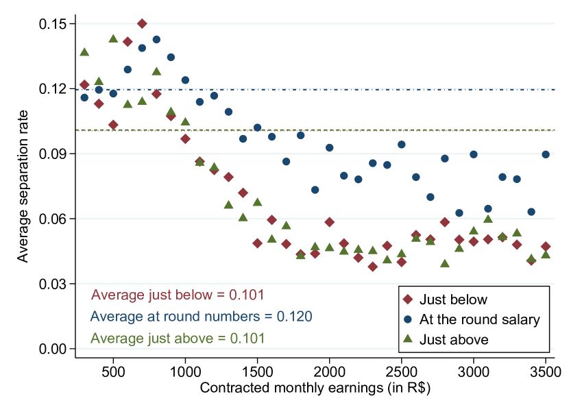
Panel A. Average resignation rate in the vicinity of round salaries

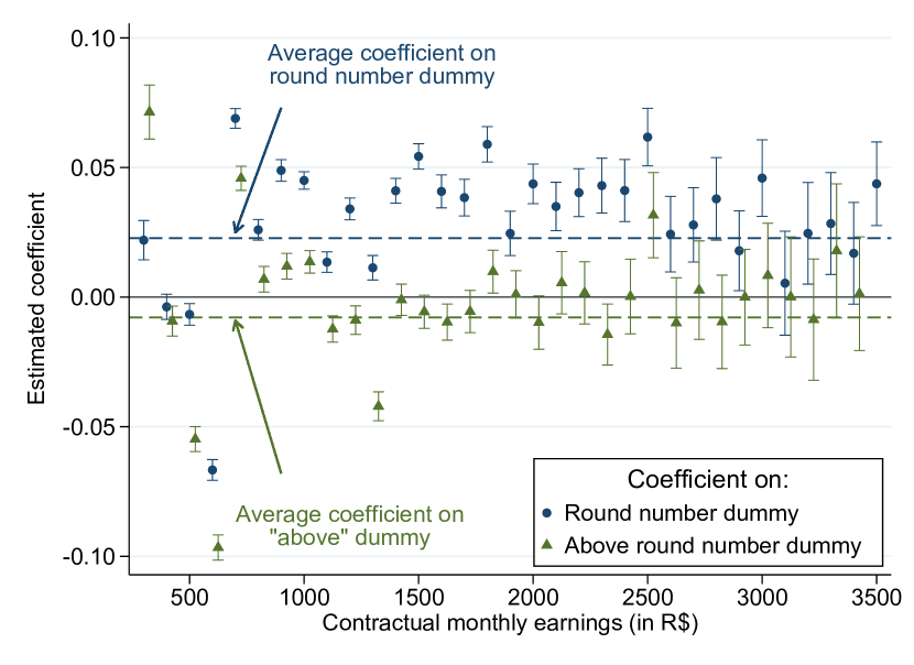
Panel B. Regression discontinuity estimates $\hat{\beta}_{r}$’s and $\hat{\gamma}_{r}$’s from equation (F.1.1)

Notes: This figure shows whether there are systematic differences in the resignation likelihood of workers earning a salary just below and just above round numbers. To construct the figures in both panels, I use the firm random sample. The figures only display workers with earnings above the minimum wage and below R$3,500 (which roughly corresponds to the 99th percentile of the earnings distribution above the minimum wage).

Panel A shows the average resignation rate of workers earning a salary just below, equal to, or just above each salary divisible by 100, using a bandwidth $h=10$. For example, the figure shows that the resignation rate of workers earning [R$490, R$500) is 4.8%, the resignation rate of workers earning R$500 is 5.3%, and the resignation rate of workers earning (R$500, R$510] is 4.4%. The horizontal dashed lines denote the weighted average resignation rate of each group of workers across all salaries divisible by 100, using the number of workers used to estimate each separation rate as the weight.

Panel B presents the RD estimates of regression (F.1.1), using as the outcome a dummy that equals one if the worker resigned and zero otherwise, and using a bandwidth $h=10$. Each point in the figure comes from a separate regression using data in the vicinity of a salary divisible by 100. For example, the point estimate at $R\$500$ uses data from workers whose earnings are within a distance $10$ of R$500 (including workers who earn exactly R$500). The vertical lines denote 95% confidence intervals using heteroskedasticity-robust standard errors. Standard errors are clustered at the worker level. The horizontal dashed line denotes the weighted average RD coefficients across all regressions, where the weights are the number of workers used to estimate each regression.

Figure F2: Difference in the number of contracts around salaries divisible by 100

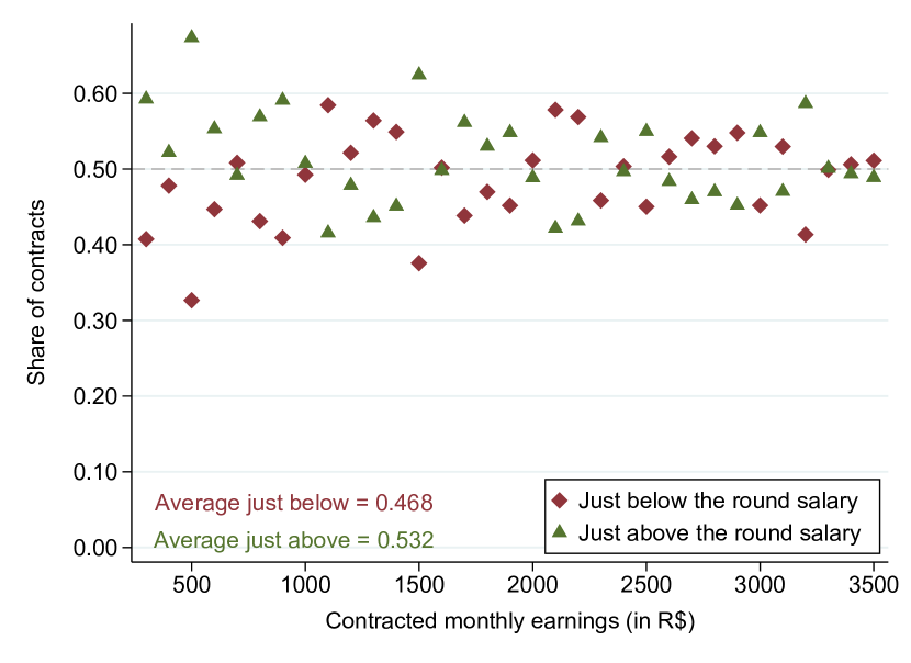
Panel A. Share of contracts just below and just above each side of the round salary

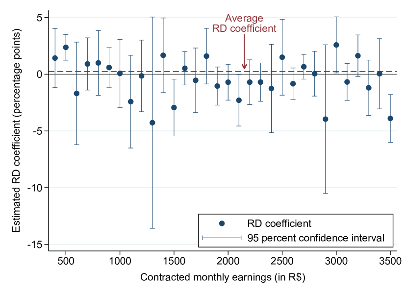
Panel B. Regression discontinuity estimates $\hat{\beta}_{r}$’s from equation (F2)

Notes: Panel A shows the fraction of contracts accrued by workers earning a salary just below and just above each salary divisible by 100, using a bandwidth $h=10$. For example, the figure shows that approximately 48% of all workers earning [R$490, R$510] - {R$500} are contracts just below R$500, that is, workers earning [R$490, R$500), while the other 52% come from above R$500, i.e., workers earning (R$500, R$510]. If workers’ earnings were uniformly distributed, the share of each side would be 50%.

Panel B presents the RD estimates of regression (F2), using as outcome variable the fraction of workers in each salary bin and a bandwidth $h=10$. Each point in the figure comes from a separate regression using data in the vicinity of a salary divisible by 100. For example, the point estimate at $R\$500$ uses data from workers whose earnings are within a distance $10$ of R$500 (excluding workers who earn exactly R$500). The vertical lines denote 95% confidence intervals using heteroskedasticity-robust standard errors. The horizontal red dashed line denotes the weighted average RD coefficient across all regressions, where the weights are the number of workers used to estimate each coefficient.

To construct the figures in both panels, I use the new-hires sample. The figures only display workers with earnings above the minimum wage and below R$3,500 (which roughly corresponds to the 99th percentile of the earnings distribution above the minimum wage).

Figure F3: Fraction of workers hired at a coarse salary across industries and occupations

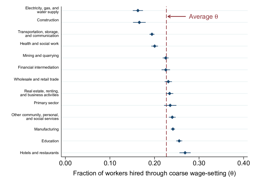
Panel A. Industry level

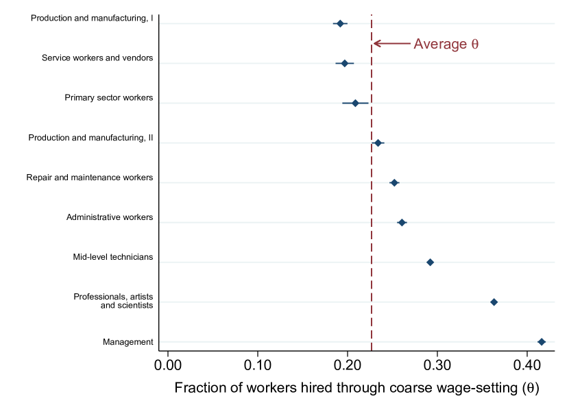
Panel B. Occupation level

Notes: This figure shows the estimated fraction of workers hired at a coarse salary across two-digit industries (Panel A) and occupations (Panel B). To construct this figure, I estimate $\hat{\theta}$ conditioning on the firm industry (Panel A) or the occupation of the new hire (Panel B), following the methodology described in Section LABEL:sub:bunching. Horizontal lines represent 95% confidence intervals. The vertical dashed red line displays the unconditional fraction of workers hired at a coarse salary.

Notes: This figure shows the estimated fraction of workers through coarse wage-setting for firms that did/did not sign a collective bargaining agreement (CBA) during 2008–2017. To construct this figure, I estimate $\hat{\theta}$ conditioning on a firm signing a CBA following the methodology described in Section LABEL:sub:bunching. Vertical lines represent 95% confidence intervals.

Notes: This figure shows the estimated fraction of workers through coarse wage-setting across firms of different sizes. To construct this figure, I estimate $\hat{\theta}$ conditioning on firm size following the methodology described in Section LABEL:sub:bunching. Vertical lines represent 95% confidence intervals.

Notes: This figure shows the distribution of contracted salaries in the new-hires sample during 2015. Red dashed lines indicate kinks in the personal income tax rate during 2015. To construct this figure, I first group workers in R$1 bins and then count the number of workers in each bin. Workers whose contracted salary is a round number are denoted with colored markers. The figure only displays workers with earnings above the minimum wage and below R$3,500 (which roughly corresponds to the 99th percentile of the distribution of earnings above the minimum wage). See Appendix D for the sample restrictions.

Appendix G Changes in the Minimum Wage and Coarse Wage-Setting

In this Appendix, I study how coarse wage-setting interacts with changes in the minimum wage (MW). dube_monopsony_2020 note that whenever a minimum wage is equal to a round number, two types of firms hire at the minimum wage: those that are constrained by the wage floor and those that are misoptimizing with respect to wages and pay the minimum wage because it is a round number. An increase in the minimum wage affects both types of firms and possibly causes the second type of firm to fully optimize wages. A similar logic follows for firms that pay a round-numbered wage below the new minimum wage.

I observe hiring decisions under fifteen different federal minimum wages, seven of which are round numbers (see Appendix Table LABEL:tab_min_wages). I also observe the year $t+1$ salary of workers hired in year $t$. Thus, to shed light on this potential spillover effect, I analyze the fraction of workers who earn a non-round salary in year $t+1$ as a function of the salary at which they were hired.

Table LABEL:tab_mw_spillover summarizes all possible wage transitions. Panel A shows the transitions for workers that were hired at the minimum wage, $w_{t}=$ MW_t; Panel B for workers hired at a wage above the minimum wage, but below the minimum wage of the following year, $w_{t}\in($MW${}_{t},$ MW${}_{t+1})$; and Panel C for workers hired at a wage above the year $t+1$ minimum wage, $w_{t}\geq$MW_t+1. By construction, only workers in Panels A and B are directly affected by the change in the minimum wage between year $t$ and year $t+1$. Hence, the transitions in Panel C are useful as a comparison group to assess how different types of wages tend to change irrespective of the direct effect due to a change in the minimum wage.

For conciseness, I focus on how a change in the minimum wage affects the round salaries that it crosses. Panel B shows that 47.7% of the workers hired at a round salary between MW_t and MW_t+1 in year $t$ earn a non-round salary in year $t+1$ (excluding the new minimum wage). One way to benchmark this magnitude is to compare it to the fraction of workers hired at a round salary above MW_t+1 who earn a non-round salary the following year (excluding the new minimum wage). This figure equals 42.3%. This benchmark can be thought of as the counterfactual fraction of workers that would earn a non-coarse wage in year $t+1$ had the minimum wage not changed. Comparing these two transitions following a “differences-in-differences” approach, suggests that a change in the minimum wage decreases the share of coarse wages by 5.4 percentage points (or 11.3%).

An alternative comparison group is the fraction of workers hired at a non-round salary above MW_t+1 who also earn a non-round salary in year $t+1$. This figure is akin to the likelihood that a firm that optimized salaries in year $t$ also optimizes in year $t+1$. Since this benchmark uses firms that fully optimized wages in the first period, it can be thought of as an upper bound for firms that initially paid coarse wages. The second row of Panel C show that this figure is 88.3% (column 6). The increase in the minimum wage achieves 54.0% (= 47.7%/88.3%) of this benchmark.

These findings suggest that changes in the minimum wage can have sizable spillover effects on firm wage-setting behavior.